Embed Size (px)
Citation preview

Multichannel Sampling of FiniteRate of Innovation Signals
Hojjat Akhondi Asl
April 2011
A Thesis submitted in fulfilment of requirements for the degreeof Doctor of Philosophy of Imperial College London
Communications and Signal Processing GroupDepartment of Electrical and Electronic Engineering
Imperial College London

3
Abstract
Recently there has been a surge of interest in sampling theory in signal process-
ing community. New efficient sampling techniques have been developed that allow
sampling and perfectly reconstructing some classes of non-bandlimited signals at
sub-Nyquist rates. Depending on the setup used and reconstruction method in-
volved, these schemes go under different names such as compressed sensing (CS),
compressive sampling or sampling signals with finite rate of innovation (FRI).
In this thesis we focus on the theory of sampling non-bandlimited signals
with parametric structure or specifically signals with finite rate of innovation. Most
of the theory on sampling FRI signals is based on a single acquisition device with
one-dimensional (1-D) signals. In this thesis, we extend these results to the case of
2-D signals and multichannel acquisition systems. The essential issue in multichan-
nel systems is that while each channel receives the input signal, it may introduce
different unknown delays, gains or affine transformations which need to be estimated
from the samples together with the signal itself. We pose both the calibration of
the channels and the signal reconstruction stage as a parametric estimation problem
and demonstrate that a simultaneous exact synchronization of the channels and re-
construction of the FRI signal is possible. Furthermore, because in practice perfect
noise-free channels do not exist, we consider the case of noisy measurements and
show that by considering Cramer-Rao bounds as well as numerical simulations, the
multichannel systems are more resilient to noise than the single-channel ones.
Finally, we consider the problem of system identification based on the multi-

0. Abstract 4
channel and finite rate of innovation sampling techniques. First, by employing our
multichannel sampling setup, we propose a novel algorithm for system identification
problem with known input signal, that is for the case when both the input signal and
the samples are known. Then we consider the problem of blind system identification
and propose a novel algorithm for simultaneously estimating the input FRI signal
and also the unknown system using an iterative algorithm.

5
Declaration of Originality
I declare that the whole content of this thesis is the outcome and product of my
own research work under the helpful guidance and support of my supervisor, Dr Pier
Luigi Dragotti. Any ideas or quotations from the work of other people, published
or otherwise, are fully acknowledged in accordance with the standard referencing
practices of the discipline. The material of this thesis has not been submitted for
any degree at any other academic or professional institution.


7
Acknowledgment
First and foremost, I would like to deeply thank my thesis supervisor Dr. Pier Luigi
Dragotti for his unmatched support and quality supervision throughout my research
and writing-up. I have been so grateful and blessed to have a PhD supervisor whose
motivations and encouragements in our research discussions have been second-to-
none. I have known Pier Luigi since the day I started Electrical Engineering at
Imperial College London. Then, he was our Communications-I lecturer and I greatly
enjoyed his lectures with his energetic smiles and wisdom. For me, it has been an
honour to undertake my Master’s and PhD thesis under his supervision and I am
thankful for his wonderful advises in our regular weekly meetings which has ensured
my work come to a satisfactory and timely conclusion.
Despite the usual stresses, these research years have been quite enjoyable,
thanks to my friends and colleagues in the CSP group. In particular, I want to
thank Pradeep and Dushyant (Dush) for the good moments we had together during
our lunch times and coffee breaks.
Last but not least and probably most important of all, I would like to thank
my mum and dad for their self-less support and encouragement and I am especially
thankful to my dear wife Fatemeh for her constant support, patience and under-
standing.

9
Contents
Abstract 3
Acknowledgment 7
Contents 9
List of Figures 13
Abbreviations 19
Mathematical Notations 21
Chapter 1. Introduction 25
1.1 Background . . . . . . . . . . . . . . . . . . . . . . . . . . . . . . . . 25
1.2 Motivation and Problem Statement . . . . . . . . . . . . . . . . . . . 28
1.3 Organization of the Thesis . . . . . . . . . . . . . . . . . . . . . . . . 30
1.4 Original Contribution . . . . . . . . . . . . . . . . . . . . . . . . . . . 31
Chapter 2. Finite Rate of Innovation Sampling Theory 33
2.1 Introduction . . . . . . . . . . . . . . . . . . . . . . . . . . . . . . . . 33
2.2 Finite Rate of Innovation Sampling Framework . . . . . . . . . . . . 34
2.2.1 Signals with Finite Rate of Innovation . . . . . . . . . . . . . 34
2.2.2 Sampling Setup . . . . . . . . . . . . . . . . . . . . . . . . . . 35
2.2.3 Sampling Kernels . . . . . . . . . . . . . . . . . . . . . . . . . 36
2.3 Reconstruction Algorithms . . . . . . . . . . . . . . . . . . . . . . . . 40
2.4 FRI Sampling in the Presence of Noise . . . . . . . . . . . . . . . . . 47
2.4.1 Total Least-Squares Method . . . . . . . . . . . . . . . . . . . 48
2.4.2 Matrix Pencil Method . . . . . . . . . . . . . . . . . . . . . . 48
Contents 10
2.4.3 Cadzow’s Algorithm . . . . . . . . . . . . . . . . . . . . . . . 51
2.5 Summary . . . . . . . . . . . . . . . . . . . . . . . . . . . . . . . . . 52
Chapter 3. Multichannel Sampling of Finite Rate of Innovation Sig-
nals 53
3.1 Introduction . . . . . . . . . . . . . . . . . . . . . . . . . . . . . . . . 53
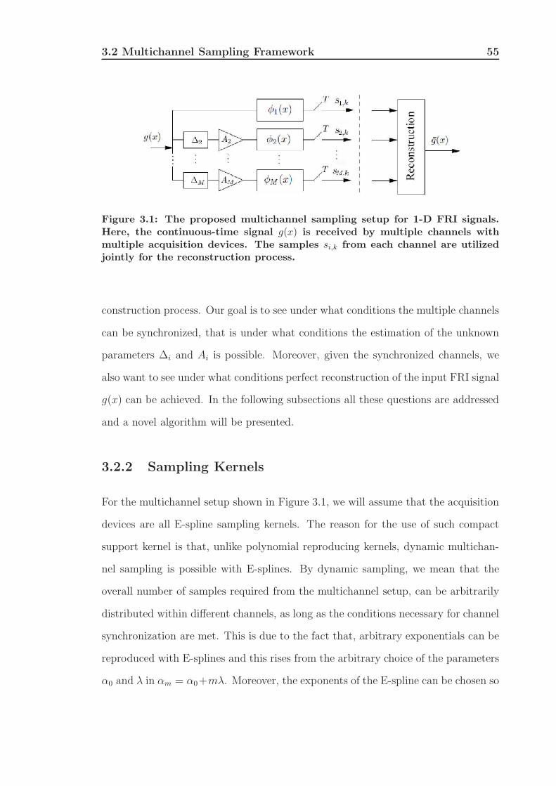
3.2 Multichannel Sampling Framework . . . . . . . . . . . . . . . . . . . 54
3.2.1 Sampling Setup . . . . . . . . . . . . . . . . . . . . . . . . . . 54
3.2.2 Sampling Kernels . . . . . . . . . . . . . . . . . . . . . . . . . 55
3.3 Multichannel Sampling of Finite Rate of Innovation Signals . . . . . . 56
3.3.1 Channel Synchronization . . . . . . . . . . . . . . . . . . . . . 56
3.3.2 Signal Reconstruction . . . . . . . . . . . . . . . . . . . . . . 58
3.3.3 Generalization . . . . . . . . . . . . . . . . . . . . . . . . . . . 59
3.4 Noisy Scenario . . . . . . . . . . . . . . . . . . . . . . . . . . . . . . 61
3.5 Multichannel Sampling of FRI Signals in the Presence of Noise . . . . 62
3.5.1 Simulation Results . . . . . . . . . . . . . . . . . . . . . . . . 64
3.6 Summary . . . . . . . . . . . . . . . . . . . . . . . . . . . . . . . . . 67
Chapter 4. System Identification based on the Theories of Finite Rate
of Innovation Sampling 69
4.1 Introduction . . . . . . . . . . . . . . . . . . . . . . . . . . . . . . . . 69
4.2 System Identification with Known Input Signal . . . . . . . . . . . . 71
4.2.1 Identification of a System with K Diracs . . . . . . . . . . . . 73
4.2.2 B-Splines . . . . . . . . . . . . . . . . . . . . . . . . . . . . . 75
4.2.3 E-Splines . . . . . . . . . . . . . . . . . . . . . . . . . . . . . 78
4.2.4 Linear Time-Invariant Circuits . . . . . . . . . . . . . . . . . . 80
4.3 Blind System Identification . . . . . . . . . . . . . . . . . . . . . . . . 83
4.4 Summary . . . . . . . . . . . . . . . . . . . . . . . . . . . . . . . . . 87
Chapter 5. Multichannel Sampling of Multidimensional FRI Signals 89
5.1 Introduction . . . . . . . . . . . . . . . . . . . . . . . . . . . . . . . . 89
5.2 Multidimensional Sampling Framework . . . . . . . . . . . . . . . . . 90
5.2.1 2-D Signals with Finite Rate of Innovation . . . . . . . . . . . 90
5.2.2 Sampling Setup . . . . . . . . . . . . . . . . . . . . . . . . . . 91
5.2.3 Multidimensional Sampling Kernels . . . . . . . . . . . . . . . 92
Contents 11
5.2.4 Geometric and Exponential Moments . . . . . . . . . . . . . . 94
5.3 Reconstruction Techniques . . . . . . . . . . . . . . . . . . . . . . . . 95
5.3.1 A Sampling Theorem for 2-D Diracs . . . . . . . . . . . . . . 96
5.3.2 A Sampling Theorem for Bi-level Polygons . . . . . . . . . . . 102
5.4 Multichannel Sampling Framework . . . . . . . . . . . . . . . . . . . 106
5.4.1 Channel Synchronization and Signal Reconstruction under 2-
D Translations . . . . . . . . . . . . . . . . . . . . . . . . . . 107
5.4.2 Channel Synchronization and Signal Reconstruction under
Affine Transformation . . . . . . . . . . . . . . . . . . . . . . 109
5.5 Summary . . . . . . . . . . . . . . . . . . . . . . . . . . . . . . . . . 113
Chapter 6. Conclusion 115
6.1 Thesis Summary . . . . . . . . . . . . . . . . . . . . . . . . . . . . . 115
6.2 Future Research . . . . . . . . . . . . . . . . . . . . . . . . . . . . . . 117
Appendix A. Cramer-Rao Bound Derivation 119
Bibliography 125


13
List of Figures
1.1 The proposed multichannel sampling setup. . . . . . . . . . . . . . . 29
2.1 A typical sampling setup for 1-D FRI signals. Here, g(x) is the
continuous-time input signal, h(x) the impulse response of the acqui-
sition device, φ(x) the sampling kernel and T the sampling period.
The measured samples are sk = 〈g(x), φ(x/T − k)〉. . . . . . . . . . . 35
2.2 B-splines of orders 1, 2, 3 and 4. (a) B-spline of order 1 (b) B-spline
of order 2 (c) B-spline of order 3 (d) B-spline of order 4. . . . . . . . 38
2.3 E-splines of orders 1, 2, 3 and 4. (a) E-spline of order 1 with α0 =
−0.2+0.3j (b) E-spline of order 2 with α0:1 = [−0.2+0.3j,−0.1+0.1j]
(c) E-spline of order 3 with α0:2 = [−0.2 + 0.3j,−0.1 + 0.1j, 0.5] (d)
E-spline of order 4 with α0:3 = [−0.2+0.3j,−0.1+0.1j, 0.5, 0.2−0.1j].
The blue and red lines show the real and imaginary parts of the E-
splines respectively. . . . . . . . . . . . . . . . . . . . . . . . . . . . . 41
2.4 FRI sampling setup with possible sources of noise in the entire sam-
pling process. . . . . . . . . . . . . . . . . . . . . . . . . . . . . . . . 47
3.1 The proposed multichannel sampling setup for 1-D FRI signals. Here,
the continuous-time signal g(x) is received by multiple channels with
multiple acquisition devices. The samples si,k from each channel are
utilized jointly for the reconstruction process. . . . . . . . . . . . . . 55

List of Figures 14
3.2 Multichannel sampling with M = 2 versus single-channel sampling.
(a) Single-channel sampling of 8 Diracs with N = 20 samples taken.
(b) Multichannel sampling of the same signal with N = 20 samples
taken for each channel, M = 2, A2 = 2 and ∆2 = 0.1s. In both
figures, Diracs with circles on top are the true locations and Diracs
with asterisks on top are the reconstructed Diracs. . . . . . . . . . . . 60
3.3 Multichannel sampling region with M = 2. Here, Q1 and Q2 repre-
sent the E-spline sampling kernel order for each channel. . . . . . . . 61
3.4 CRB for single-channel and multichannel sampling systems. The in-
put SNR is calculated as 10log10||sk||
2
σ2 where σ2 is the noise variance
and ∆t is the uncertainty on the estimated locations. Dirac locations
are set at 0.5, 0.6 and 0.7 for all cases. The delays ∆2 and ∆3 are
fixed at T2and T respectively. . . . . . . . . . . . . . . . . . . . . . . 64
3.5 Theoretical uncertainties on the estimated locations with varying
sampling rates. The input SNR is calculated as 10log10||sk||
2
σ2 where
σ2 is the noise variance and ∆t is the uncertainty on the estimated
locations. Dirac locations are set at 0.5, 0.6 and 0.7 for all cases. The
delays ∆2 and ∆3 are fixed at T2and T respectively. . . . . . . . . . . 65
3.6 Numerical results with single and multichannel sampling. The input
SNR is calculated as 10log10||sk||
2
σ2 where σ2 is the noise variance and
∆t is the uncertainty on the estimated locations. Dirac locations are
set at 0.5, 0.6 and 0.7 for all cases. The delays ∆2 and ∆3 are fixed
at T2and T respectively. . . . . . . . . . . . . . . . . . . . . . . . . . 66
4.1 A system identification problem setup. Here, g(x) represents the
continuous-time input signal, ψ(x) represents the unknown system
and sk represent the output samples . . . . . . . . . . . . . . . . . . . 70

List of Figures 15
4.2 System identification setup with known input signal g(x). Here, the
function φ(x), identical in both channels, represents the E-spline sam-
pling kernel and the output samples sSIGk and sSY Sk represent the sig-
nal and the system samples respectively. . . . . . . . . . . . . . . . . 71
4.3 System identification of an unknown system ψ(x) consisting of 3
Diracs. (a) The input piecewise-polynomial signal. (b) The true
parameters of the function ψ(x). (c) Input signal convolved with the
function ψ(x). (d) The real (blue) and imaginary (red) samples of
the signal. (e) The real (blue) and imaginary (red) samples of the
system. (f) Estimated parameters of the function ψ(x). . . . . . . . . 75
4.4 System identification of an unknown system ψ(x) with a B-spline of
order 4. (a) The input signal with 2 Diracs. (b) The true values of
the function ψ(x). (c) Input signal convolved with the function ψ(x).
(d) The real (blue) and imaginary (red) samples of the signal. (e)
The real (blue) and imaginary (red) samples of the system. (f) The
estimated function ψ(x). . . . . . . . . . . . . . . . . . . . . . . . . . 77
4.5 System identification of an unknown system ψ(x) with an E-spline of
order 2 and parameters γ0 = −1 and γ1 = 2. (a) The input signal with
2 Diracs. (b) The true values of the function ψ(x). (c) Input signal
convolved with the function ψ(x). (d) The real (blue) and imaginary
(red) samples of the signal. (e) The real (blue) and imaginary (red)
samples of the system. (f) The estimated function ψ(x) with MSE of
3× 10⁻⁶ due to numerical imprecision. . . . . . . . . . . . . . . . . . 81
4.6 First order RC circuit as the unknown function ψ(x). Here, the out-
put samples sSIGk and sSY Sk represent the input signal and the system
samples respectively. . . . . . . . . . . . . . . . . . . . . . . . . . . . 82

List of Figures 16
4.7 System identification of an unknown system ψ(x) with a first order
RC circuit where γ = 1/RC = 0.5. (a) The input signal with 2
Diracs. (b) The true values of the function ψ(x). (c) Input signal
convolved with the function ψ(x). (d) The real (blue) and imaginary
(red) samples of the signal. (e) The real (blue) and imaginary (red)
samples of the system. (f) The estimated function ψ(x) with MSE of
1.3× 10⁻⁶ due to numerical imprecision. . . . . . . . . . . . . . . . . 84
4.8 The setup proposed for recursive estimation. Here, g(x) is the in-
put FRI signal, ψ(x) is the unknown system to be identified, φ(x) is
the E-spline sampling kernel, τ 0m represent the initial measurements,
τupdm represent the updated measurements,ˆψ(αm) represents the re-
estimated Fourier transform of the unknown system and g(x) repre-
sents the estimated input FRI signal. . . . . . . . . . . . . . . . . . . 85
4.9 Simultaneous estimation of an input sparse signal with a first order
E-spline as the unknown function ψ(x). (a) The input signal with 2
Diracs (circle) along with the immediate estimate of the signal (aster-
isk) with no iterations. (b) Input signal convolved with the function
ψ(x). (c) The real (blue) and imaginary (red) samples with no it-
eration. (d) The real (blue) and imaginary (red) samples after 10
iterations. (e) True vs. estimated values of the parameter γ after 10
iterations. (f) True vs. estimated version of the input signal after 10
iterations. . . . . . . . . . . . . . . . . . . . . . . . . . . . . . . . . . 86
List of Figures 17
4.10 Simultaneous estimation of an input sparse signal with a first order
RC circuit as the unknown function ψ(x). (a) The input signal with 2
Diracs (circle) along with the immediate estimate of the signal (star)
with no iterations. (b) Input signal convolved with the function ψ(x).
(c) The real (blue) and imaginary (red) samples with no iteration. (d)
The real (blue) and imaginary (red) samples after 20 iterations. (e)
True vs. estimated values of the parameter γ after 20 iterations. (f)
True vs. estimated version of the input signal after 20 iterations. . . . 88
5.1 A typical sampling setup for 2-D FRI signals. Here, g(x, y) repre-
sents the input FRI signal, φ(x, y) the sampling kernel, gs(x, y) the
sampled version of the input signal, sj,k the samples and Tx, Ty are
the sampling intervals along the Cartesian dimensions respectively. . . 91
5.2 Sampling and reconstructing a set of 2-D Diracs using E-splines (a)
The original input signal consisting of 4 Diracs in a frame size of
256 × 256. (b) The 2-D E-spline sampling kernel of order 8 along
both dimensions. (c) The 16 × 16 samples of the input signal. (d)
The reconstructed signal with the use of ACMP method. . . . . . . . 102
5.3 Sampling and reconstructing a bi-level polygon using E-splines (a)
The original input bi-level triangle (b) The 32×32 samples of the in-
put signal [not to scale] (c) The reconstructed vertices of the polygon
where the crosses are the actual vertices of the original signal. . . . . 106
5.4 The proposed multichannel sampling setup for 2-D FRI signals. The
sampling kernels φ1(x), φ2(x), . . . , φM(x) receive different geometri-
cally transformed versions of the original signal g(x, y). Here, the
unknown transformation parameters are denoted by T2, . . . , TM . . . . 107

List of Figures 18
5.5 Multichannel sampling of bi-level polygons under affine transforma-
tion. (a) The reference signal in a frame data size of 256 × 256.
(b) The affine transformed signal with (∆x,∆y) = (90,−90), θ =
50, (Xscale, Yscale) = (1.05, 1.05) and (Xshear, Yshear) = (0.5, 0.2). (c)
2-D modified E-spline sampling kernel of order 2K − 1 + 4 = 11. (d)
& (e) The 16× 16 samples of both signals. (f) & (g) K2 solutions of
both signals. (h) The reconstructed vertices of the reference signal.
The green circles are the true vertices and the white asterisks are the
mapped solutions. . . . . . . . . . . . . . . . . . . . . . . . . . . . . . 113

19
Abbreviations
FRI : Finite Rate of Innovation
CS: Compressed Sensing
ADC: Analogue-To-Digital Converter
CRB: Cramer-Rao Bound
C/D: Continuous-To-Digital
1-D: One Dimensional
2-D: Two Dimensional
E-splines: Exponential Splines
SVD: Singular-Value-Decomposition
EVD: Eigen-Value-Decomposition
SNR: Signal-To-Noise Ratio
LMS: Least Mean Square
FIR: Finite Impulse Response
ACMP: Algebraically Coupled Matrix Pencils
MEMP: Matrix Enhancement and Matrix Pencil
ECG: Electrocardiogram
RC Circuit: Circuit composed of resistors and capacitors


21
Mathematical Notations
∗ : Convolution operator
〈, 〉 : Inner product operator
BM,N : Matrix B of size M ×N
[.]T : Matrix transpose operator
[.]H : Matrix Hermitian operator
[.]−1 : Matrix inversion operator
[.]† : Matrix pseudo-inverse operator
⌈.⌉ : Ceiling operator
diag(.) : Diagonal operator
E(.) : Expectation operator
var(.) : Variance operator
||.|| : Euclidean norm operator
g(x) : Continuous-time 1-D input signal
g(x) : Estimated version of the signal g(x)
g(x, y) : Continuous domain 2-D input signal
g(jω) : Fourier transform of 1-D input signal g(x)
g(jωx, jωy) : Fourier transform of 2-D input signal g(x, y)
h(x) : Impulse response of 1-D acquisition device
h(x, y) : Impulse response of 2-D acquisition device
φ(x) : 1-D sampling kernel
0. Mathematical Notations 22
φ(x, y) : 2-D sampling kernel
φ(jω) : Fourier transform of 1-D sampling kernel φ(x)
φ(jωx, jωy) : Fourier transform of 2-D sampling kernel φ(x, y)
T : Sampling interval
(Tx, Ty) : Sampling interval along the Cartesian axes
sk : Samples of input signal g(x)
sk : Samples sk corrupted with noise
σ2 : Noise variance
ǫk : White additive Gaussian noise at the sample index k
sj,k : Samples of input signal g(x, y)
N : Total number of samples sk
(Nx, Ny) : Total number of samples sj,k along the Cartesian axes
cm,k : Coefficients of 1-D sampling kernels
cm,nj,k : Coefficients of 2-D sampling kernels
τm : Exponential or polynomial (geometric) moments in 1-D
τm,n : Exponential or polynomial moments in 2-D
ρ : Rate of innovation
K : The degrees of freedom of the input signal
L : Signal interval in 1-D
(Lx, Ly) : Signal interval in 2-D along the Cartesian axes
φ(x) : Dual function of φ(x)
Rg(x, θ) : Radon transform of input signal g(x, y)
ψ(x) : The function of the unknown system within the system identification setup
sSIGk : Samples of input signal g(x) within the system identification setup
sSY Sk : Samples of input signal convolved with the unknown system
τSIGm : Exponential moments of the input signal

0. Mathematical Notations 23
τSY Sm : Exponential moments of the convolved signal g(x) ∗ ψ(x)

25
Chapter 1
Introduction
1.1 Background
Real world signals such as for example communication signals, audio signals and
video signals are all analog signals; signals that are continuous in time and ampli-
tude. In order to process such signals, we need to convert them in discrete form.
The process in which a continuous-time signal g(x) is represented by a discrete set
of values or samples g[k], where k ∈ Z, is called “Sampling” in signal processing.
The process of sampling plays a fundamental role in modern signal processing and
communications where it is employed in majority of signal processing related ap-
plications such as computers, mobile phones, MP3 players, satellite receivers, radar
communications, complex telescopes and many more.
A typical sampling setup often used in practice is described by a pre-filtering
module together with a sampling device. The sampling device observes a filtered
version of the input analog signal g(x), where the filter h(x) is an antialiasing filter
or a sampling kernel. Depending on the application, the samples are taken at pre-
defined intervals where if the samples are taken at equal time instances, that is,
g[k] = g(kT ) for every T seconds, then the signal is uniformly sampled. When
1.1 Background 26
the samples are not taken at equal time instances but at arbitrary points, then we
call this form of sampling, non-uniform [51]. Considering that the sampling devices
takes uniform samples from the observed signal, the samples g[k] will be given by:
g[k] = gs(kT )
= g(x) ∗ h(x)|x=kT ,
where gs(x) is the filtered signal observed by the sampling device and ∗ denotes
the convolution operator. Given the samples, the fundamental questions of inter-
est for such a process are, 1) Under what conditions signal g(x) is perfectly and
uniquely recovered from the set of samples g[k] and 2) What are the methods of
reconstruction?
The classical yet powerful answer to these key questions was given by Whit-
taker [85], Kotel’nikov [39, 40], and Shannon [67], in a well-known sampling theo-
rem1, which states that any bandlimited continuous-time signal g(x) can be perfectly
reconstructed from its samples, if the sampling rate is chosen to be equal or greater
than twice the maximum non-zero frequency of the signal2. If this condition is met,
then the reconstruction of the bandlimited signal from its samples can be obtained
with a sinc interpolation function.
This extremely fruitful result however, has two major drawbacks. First, real
world signals are never exactly bandlimited and second, an ideal sinc interpolation
function is physically not implementable. Thus, different approximations need to
be taken into account for such a sampling scheme to be used in practice [74, 37,
76]. These limitations have led researchers to re-examine some of the core ideas
of the classical sampling theory and take it further into more advanced sampling
techniques, including extensions to a larger class of signals that are not necessarily
1From here on, we will be referring to the theorem as Shannon’s sampling theory.2This is also referred to as Nyquist rate [56].

1.1 Background 27
bandlimited.
Recently in [25, 17, 84], it has been shown that it is possible to sample and
perfectly reconstruct some classes of non-bandlimited signals. In these schemes, the
prior that the signal is sparse in a basis or in a parametric space is taken into account
and perfect reconstruction is achieved based on a set of suitable measurements.
Depending on the setup used and reconstruction method involved, these sampling
methods go under different names such as compressed sensing (CS), compressive
sampling [25, 17, 10] or sampling signals with finite rate of innovation (FRI) [84, 52,
27].
Signals with finite rate of innovation, first introduced by Vetterli et al. in [84],
are parametric non-bandlimited signals that posses a finite number of parameters
per unit of time or, as mentioned in [84], they posses a finite number of degrees of
freedom per unit of time. Some examples of FRI signals include streams of Diracs,
piecewise-polynomial [84, 27] and piecewise-sinusoidal signals [11]. The reconstruc-
tion of these FRI signals is based on the annihilating filter method (also known
as Prony’s method [70]). More recently, the extensions to the sampling of multi-
dimensional FRI signals have been considered in [48, 47] and [69] where sampling
schemes for 2-D FRI signals, such as set of 2-D Diracs and bi-level polygons have
been presented. In-depth discussions of sampling 2-D FRI signals can be found in
[46] and [68].
The core idea behind the sampling theory of FRI signals can be thought of an
estimation problem where by recovering the degrees of freedom of the signal from
its samples, the original signal can be perfectly recovered. The sampling theory
introduced in [84], assumes a prior knowledge of the acquisition device employed,
i.e. its sampling kernel. The sampling kernels considered in [84], are infinite-support
kernels, however, it has been shown in [27] that many 1-D FRI signals with local
finite rate of innovation can be sampled and perfectly reconstructed using a wide
1.2 Motivation and Problem Statement 28
range of sampling kernels that have finite support. Such kernels have the property
of reproducing polynomials or exponentials and deliver practical implementation of
the same sampling and retrieval techniques used in [84].
1.2 Motivation and Problem Statement
The process of sampling has allowed us to manipulate, store and transmit vast
amount of data with increasing convenience. However, in data-intensive and/or
power-limited applications such as sensor networks, the information contained is
normally far less than the data observed, therefore, efficient sampling techniques
is vital and necessary in such applications. Sparse sampling theories [25, 17, 84]
are considered to be in the category of efficient sampling techniques as they allow
sub-Nyquist sampling rates while achieving perfect retrieval of the observed signal.
However, most of the papers on sparse sampling and in particular FRI sampling
focus on a single-channel acquisition model and this normally requires expensive
acquisition devices working at high sampling rates. On the contrary, multichannel
sampling allows a reduction in the complexity of the acquisition device while keeping
higher rates of conversion. For example, modern and fast Analogue-to-Digital Con-
verters (ADC) use a parallel array of lower-rate ADCs working in a time-interleaved
fashion [12]. Sensor networks and acquisition of images in a multi-camera system
are other examples of multichannel systems where highly efficient sampling schemes
are of interest. Therefore, given the practical importance of multichannel acquisi-
tion devices, it is natural to investigate extensions of sparse sampling theories to the
multichannel scenario.
In this thesis we present a possible extension of the theory of sampling sig-
nals with finite rate of innovation to the case of multichannel acquisition systems.
The critical issue in our proposed multichannel sampling setup, shown in Figure
1.2 Motivation and Problem Statement 29
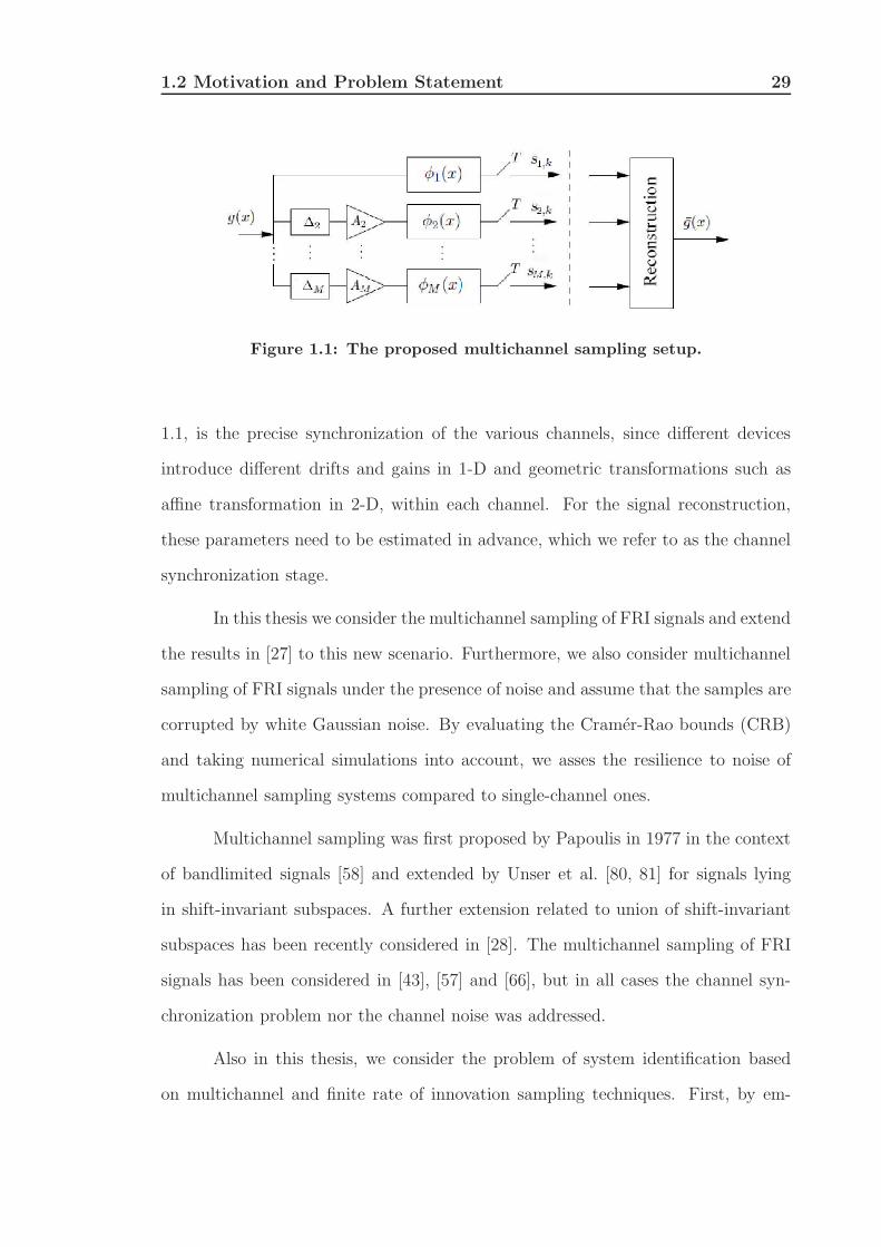
Figure 1.1: The proposed multichannel sampling setup.
1.1, is the precise synchronization of the various channels, since different devices
introduce different drifts and gains in 1-D and geometric transformations such as
affine transformation in 2-D, within each channel. For the signal reconstruction,
these parameters need to be estimated in advance, which we refer to as the channel
synchronization stage.
In this thesis we consider the multichannel sampling of FRI signals and extend
the results in [27] to this new scenario. Furthermore, we also consider multichannel
sampling of FRI signals under the presence of noise and assume that the samples are
corrupted by white Gaussian noise. By evaluating the Cramer-Rao bounds (CRB)
and taking numerical simulations into account, we asses the resilience to noise of
multichannel sampling systems compared to single-channel ones.
Multichannel sampling was first proposed by Papoulis in 1977 in the context
of bandlimited signals [58] and extended by Unser et al. [80, 81] for signals lying
in shift-invariant subspaces. A further extension related to union of shift-invariant
subspaces has been recently considered in [28]. The multichannel sampling of FRI
signals has been considered in [43], [57] and [66], but in all cases the channel syn-
chronization problem nor the channel noise was addressed.
Also in this thesis, we consider the problem of system identification based
on multichannel and finite rate of innovation sampling techniques. First, by em-

1.3 Organization of the Thesis 30
ploying our multichannel sampling setup, we propose a novel algorithm for system
identification problem with known input signal, that is for the case when both the
input signal and the samples are known. Then we consider the problem of blind
system identification and propose a novel algorithm for simultaneously estimating
the unknown system as well as the input FRI signal using an iterative algorithm.
1.3 Organization of the Thesis
The organization of this thesis is as follows:
In Chapter 2, we provide a background on FRI sampling theory where we
present and discuss the different elements of the sampling setup used for sampling
1-D FRI signals, including the sampling kernels and the reconstruction methods
involved. In this chapter, we also consider the case of noisy measurements and
discuss the common methods and tools involved for retrieving FRI signals from
noisy samples.
In Chapter 3, we present a possible extension of sampling 1-D FRI signals
to the case of multichannel sampling. In this chapter, by considering both the syn-
chronization stage and the signal reconstruction stage as a parametric estimation
problem, we propose our novel algorithm for multichannel sampling of FRI signals
and demonstrate that it is possible to estimate simultaneously the channel param-
eters (i.e., delays and gains) and the signal itself from the measured samples. Then
we consider the noisy scenario and assume that the noise samples are corrupted by
additive white Gaussian noise. By evaluating the Cramer-Rao bounds and taking
numerical simulations into account, we asses the resilience to noise of multichannel
sampling systems compared to single-channel ones.
In Chapter 4, we propose our novel algorithms for system identification based
on the theories of FRI sampling. The novelty of this chapter is divided into two
1.4 Original Contribution 31
sections; first, by employing the multichannel sampling setup presented in Chapter
3, we propose a novel algorithm for system identification problem with known input
signal. Then we consider the problem of blind system identification where by blind
we mean that only the output samples are given and the input signal is not known.
We will propose a novel algorithm for simultaneously estimating the input FRI signal
and also the unknown system using an iterative algorithm.
In Chapter 5, we consider the problem of multichannel sampling of multi-
dimensional FRI signals. In this chapter, we first introduce the multidimensional
sampling framework for FRI signals which include the definition of 2-D FRI signals,
sampling setup used and the properties of the sampling kernels involved. We then
introduce our novel algorithms for sampling and perfectly reconstructing set of 2-D
Diracs and bi-level polygons using exponential splines. Finally, we will extend the
multichannel sampling setup presented in Chapter 3, to the case of multichannel
sampling of 2-D FRI signals and present our novel algorithm for signal and channel
estimation under simple 2-D translations and also affine transformations.
We finally conclude in Chapter 6, and present some ideas and remarks for
future works.
1.4 Original Contribution
The main contribution of this thesis is the extension of finite rate of innovation
sampling to the case of multichannel sampling along with channel synchronization,
both in 1-D and 2-D. Furthermore, as the channel synchronization stage could be
thought of a system identification problem, we also consider the problem of system
identification based on FRI sampling techniques and propose a novel algorithm for
identifying unknown systems by employing a FRI sampling setup.
To the best of our knowledge, Chapters 3, 4 and 5 contain original research

1.4 Original Contribution 32
work where these contributions have led to the following publications:
• H. Akhondi Asl and P.L. Dragotti. Simultaneous Estimation of Sparse
Signals and Systems at sub-Nyquist Rates. To appear in the 19th Eu-
ropean Signal Processing Conference (EUSIPCO11), Barcelona, Spain, 2011.
• H. Akhondi Asl and P.L. Dragotti. Multichannel Sampling of Multidi-
mensional Parametric Signals. To appear in the special issue of Sampling
Theory in Signal and Image Processing Journal, 2011.
• H. Akhondi Asl and P.L. Dragotti and L. Baboulaz. Multichannel Sam-
pling of Signals with Finite Rate of Innovation. IEEE Signal Processing
Letters, vol.17, no.8, pp.762-765, August 2010.
• H. Akhondi Asl and P.L. Dragotti. Multichannel Sampling of Translated,
Rotated and Scaled Bi-level Polygons using Exponential Splines. 8th
International Conference on Sampling Theory and Applications (SAMPTA09),
Marseille, France, May 2009.
• H. Akhondi Asl and P.L. Dragotti. Single and Multichannel Sampling
of Bi-level Polygons using Exponential Splines. IEEE International
Conference on Acoustics, Speech and Signal Processing (ICASSP09), Taipei,
Taiwan, April 2009.
• H. Akhondi Asl and P.L. Dragotti. A Sampling Theorem For Bi-level
Polygons using E-Splines, 8th International Conference on Mathematics
in Signal Processing (IMA08), Royal Agriculture College, Cirencester, UK,
December 2008.
33
Chapter 2
Finite Rate of Innovation
Sampling Theory
2.1 Introduction
In 2002, Vetterli et al. [84] introduced the notion of signals with finite rate of
innovation. In their work, they showed that it is possible to sample and perfectly
reconstruct some classes of signals that are neither bandlimited nor belong to a fixed
subspace. Signals that can be reconstructed using this framework are called signals
with finite rate of innovation (FRI) as they can be completely defined by a finite
number of parameters per unit of time.
Since its introduction in 2002, finite rate of innovation sampling is finding
more and more applications, for example, for compression of ECG signals [31], res-
olution enhancement [27, 52], distributed compression [30, 18], synchronization and
channel estimation for ultra-wideband signals [46, 50, 42], ADC converters [38] and
image super-resolution [7, 8, 9].
In this chapter we provide a background on finite rate of innovation sampling
theory which is the core foundation of this thesis. The organization of this chapter

2.2 Finite Rate of Innovation Sampling Framework 34
is as follows: In Section 2.2 we start by presenting a mathematical definition for 1-D
FRI signals. Then, the different elements of the sampling setup used for sampling
1-D FRI signals, including the sampling kernels and the reconstruction methods
involved will be presented and fully discussed. In Section 2.4, we will consider
the case of noisy scenario and present and discuss the common methods and tools
involved for retrieving FRI signals from noisy samples. We will finally conclude with
a summary at the end of this chapter.
2.2 Finite Rate of Innovation Sampling Frame-
work
2.2.1 Signals with Finite Rate of Innovation
Let us consider a 1-D signal of the form [27]:
g(x) =N∑
r=0
∑
j∈Z
γj,r φr(x− xj). (2.1)
The degrees of freedom of the signal g(x) are the shifts xj and the coefficients γj,r,
assuming that the set of functions φr(x) are known. If we introduce a counting
function Cg(xa, xb) which counts the number of free parameters of g(x) over the
interval L = [xa, xb], then the rate of innovation ρ of the signal g(x) is defined as:
ρ = limL→∞
1
LCg(−L/2, L/2). (2.2)
If ρ is finite, then the signal is said to have a finite rate of innovation. It is important
to note that all shift-invariant signals, including bandlimited signals can be defined
with the above definition. The rate of innovation of real-valued bandlimited signals
is: ρ = 2× fmax where fmax is the maximum frequency of the bandlimited signal.
2.2 Finite Rate of Innovation Sampling Framework 35
2.2.2 Sampling Setup
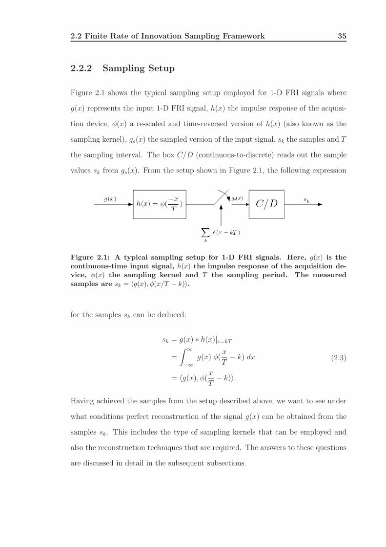
Figure 2.1 shows the typical sampling setup employed for 1-D FRI signals where
g(x) represents the input 1-D FRI signal, h(x) the impulse response of the acquisi-
tion device, φ(x) a re-scaled and time-reversed version of h(x) (also known as the
sampling kernel), gs(x) the sampled version of the input signal, sk the samples and T
the sampling interval. The box C/D (continuous-to-discrete) reads out the sample
values sk from gs(x). From the setup shown in Figure 2.1, the following expression
Figure 2.1: A typical sampling setup for 1-D FRI signals. Here, g(x) is thecontinuous-time input signal, h(x) the impulse response of the acquisition de-vice, φ(x) the sampling kernel and T the sampling period. The measuredsamples are sk = 〈g(x), φ(x/T − k)〉.
for the samples sk can be deduced:
sk = g(x) ∗ h(x)|x=kT
=
∫ ∞
−∞
g(x) φ(x
T− k) dx
= 〈g(x), φ(xT
− k)〉.
(2.3)
Having achieved the samples from the setup described above, we want to see under
what conditions perfect reconstruction of the signal g(x) can be obtained from the
samples sk. This includes the type of sampling kernels that can be employed and
also the reconstruction techniques that are required. The answers to these questions
are discussed in detail in the subsequent subsections.
2.2 Finite Rate of Innovation Sampling Framework 36
2.2.3 Sampling Kernels
Sampling kernels are characterized by the physical properties of the acquisition
device which are normally specified and cannot be modified. Unlike the classical
sampling schemes, FRI sampling schemes provide a larger choice of kernels that
allow perfect reconstruction of the input signal. The sampling kernels considered
in [84] are the sinc and the Gaussian kernels. Such kernels have an infinite support
and are therefore not physically realizable. Moreover, the use of such kernels make
the reconstruction algorithm unstable. Dragotti et al. [27] showed that FRI signals
with local finite rate of innovation can be sampled and reconstructed using a wide
range of sampling kernels that have finite support. Such kernels have the property
of reproducing polynomials or exponentials and deliver practical implementation of
the same sampling and retrieval techniques used in [84] for 1-D FRI signals.
In this thesis, we will focus on polynomial and exponential reproducing ker-
nels and in particular exponential splines (E-splines) [79, 75], splines that can repro-
duce real or complex exponentials. E-splines are compact support splines that are
practically implementable (using RC circuits for example [27]) and our simulation
results show that they tend to be more stable than other kernels.
Polynomial Reproducing Kernels
Any kernel φ(x) that together with its shifted versions can reproduce polynomials
of maximum degreeM is called a polynomial reproducing kernel. That is any kernel
satisfying the following property:
∑
k∈Z
cm,kφ(x− k) = xm, (2.4)
for a proper choice of coefficients cm,k with m = 0, 1, . . . ,M . Here, the subscript k
represents the shifts index and the superscript m represents the polynomial degree.
2.2 Finite Rate of Innovation Sampling Framework 37
The choice of M depends on the local rate of innovation of the signal g(x) and will
be discussed later on. Furthermore, the coefficients cm,k can be calculated as follows:
cm,k =
∫ ∞
−∞
xmφ(x− k) dx, (2.5)
where φ(x) is chosen to form with φ(x) a quasi-biorthonormal set [15]. This includes
the particular case where φ(x) is the dual of φ(x), that is, 〈φ(x−j), φ(x−k)〉 = δj,k.
We should mention that, given the specified kernel and the required polynomial
degree, the coefficients can also be calculated numerically.
Polynomial reproducing kernels include any function satisfying the so-called
Strang-Fix conditions [71] which states that, the kernel φ(x) satisfies Equation (2.4)
if and only if its Fourier transform φ(jω) satisfies:
φ(0) 6= 0 and,
φ(m)(2kπ) = 0 for k 6= 0 and m = 0, 1, . . . ,M,
(2.6)
where the superscript (m) stands for the m-th order derivative of φ(jω). B-splines
[77, 78, 73] are one of the most well-known examples of kernels satisfying the Strang-
Fix conditions. A function β(x) with Fourier transform:
βM(jω) =M∏
m=0
1− e−jω
jω, (2.7)
is called a B-spline of order M + 1. The resulting spline has compact support and
can reproduce any polynomial in the subspace spanned by 1, x, x2, . . . , xM. In the
time-domain, the expression of a B-spline of order 1 is given as follows:
β0(x) =
1 0 ≤ x < 1
0 otherwise,
(2.8)
2.2 Finite Rate of Innovation Sampling Framework 38
and the higher order B-spline functions are obtained by successive convolutions of
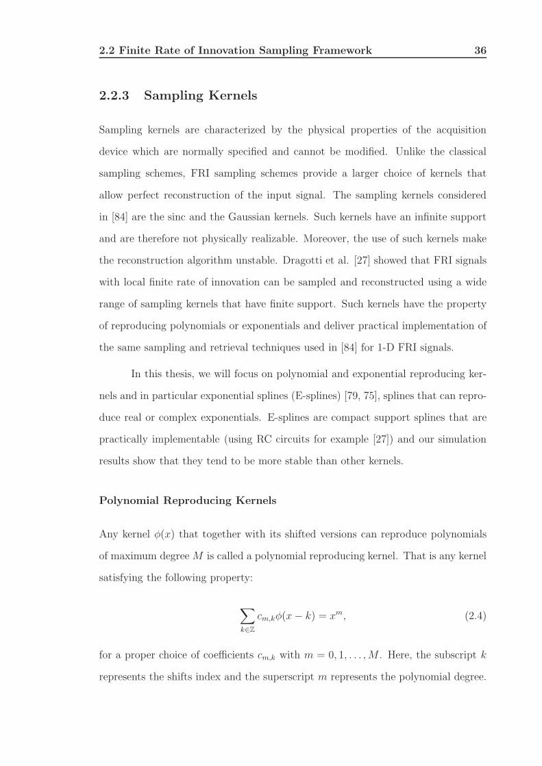
the first order B-spline, defined above. B-splines are biorthogonal functions and
their dual basis is defined in [65]. Figures 2.2(a)(b)(c) and (d) show B-splines of
order 1, 2, 3 and 4 respectively.
(a) (b)
(c) (d)
Figure 2.2: B-splines of orders 1, 2, 3 and 4. (a) B-spline of order 1 (b) B-splineof order 2 (c) B-spline of order 3 (d) B-spline of order 4.
Strang-Fix conditions are also used extensively in wavelet theory and
Daubechies scaling functions satisfy such conditions [20, 83]. More precisely, a
wavelet with M + 1 vanishing moments is generated by a scaling function that can
reproduce polynomials of degree M . Daubechies scaling functions are orthogonal
functions, and their dual basis is: φ(x) = φ(x).
2.2 Finite Rate of Innovation Sampling Framework 39
Exponential Reproducing Kernels
Any kernel φ(x) that together with its shifted versions can reproduce real or com-
plex exponentials of the form eαmx with m = 0, 1, . . . ,M is called an exponential
reproducing kernel. That is any kernel satisfying the following property:
∑
k∈Z
cm,kφ(x− k) = eαmx, with αm ∈ C, (2.9)
for a proper choice of coefficients cm,k ∈ C. The coefficients cm,k in the above
equation are given by the following expression:
cm,k =
∫ ∞
−∞
eαmxφ(x− k)dx, (2.10)
where, as in the polynomial reproducing kernel’s case, φ(x) is chosen to form with
φ(x) a quasi-biorthonormal set. The choice of the exponents in Equation (2.9) is
restricted to αm = α0 + mλ with α0, λ ∈ C and m = 0, 1, ...,M . This is done to
allow the use of the annihilating filter method at the reconstruction stage. This fact
will be more evident when the reconstruction methods are described later on.
The theory of exponential reproducing kernels is quite recent and is based on
the notion of E-splines [79]. A function β~α(x) with Fourier transform:
β~α(jω) =
M∏
m=0
1− eαm−jω
jω − αm
, (2.11)
is called an E-spline of orderM+1 where ~α = (α0, α1, . . . , αM). The produced spline
has compact support and can reproduce any exponential in the subspace spanned
by (eα0x, eα1x, . . . , eαMx). Moreover, the values of α0 and λ can be chosen arbitrarily,
but too small or too large values could lead to unstable results for the reproduction
of exponentials. In the time-domain, the expression of an E-spline of order one is
2.3 Reconstruction Algorithms 40
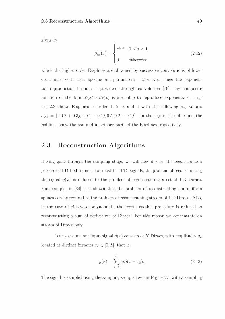
given by:
βα0(x) =
eα0x 0 ≤ x < 1
0 otherwise,
(2.12)
where the higher order E-splines are obtained by successive convolutions of lower
order ones with their specific αm parameters. Moreover, since the exponen-
tial reproduction formula is preserved through convolution [79], any composite
function of the form φ(x) ∗ β~α(x) is also able to reproduce exponentials. Fig-
ure 2.3 shows E-splines of order 1, 2, 3 and 4 with the following αm values:
α0:3 = [−0.2 + 0.3j,−0.1 + 0.1j, 0.5, 0.2 − 0.1j]. In the figure, the blue and the
red lines show the real and imaginary parts of the E-splines respectively.
2.3 Reconstruction Algorithms
Having gone through the sampling stage, we will now discuss the reconstruction
process of 1-D FRI signals. For most 1-D FRI signals, the problem of reconstructing
the signal g(x) is reduced to the problem of reconstructing a set of 1-D Diracs.
For example, in [84] it is shown that the problem of reconstructing non-uniform
splines can be reduced to the problem of reconstructing stream of 1-D Diracs. Also,
in the case of piecewise polynomials, the reconstruction procedure is reduced to
reconstructing a sum of derivatives of Diracs. For this reason we concentrate on
stream of Diracs only.
Let us assume our input signal g(x) consists of K Diracs, with amplitudes ak
located at distinct instants xk ∈ [0, L[, that is:
g(x) =K∑
k=1
akδ(x− xk). (2.13)
The signal is sampled using the sampling setup shown in Figure 2.1 with a sampling
2.3 Reconstruction Algorithms 41
(a) (b)
(c) (d)
Figure 2.3: E-splines of orders 1, 2, 3 and 4. (a) E-spline of order 1 with α0 =−0.2+0.3j (b) E-spline of order 2 with α0:1 = [−0.2+0.3j,−0.1+0.1j] (c) E-splineof order 3 with α0:2 = [−0.2 + 0.3j,−0.1 + 0.1j, 0.5] (d) E-spline of order 4 withα0:3 = [−0.2+0.3j,−0.1+0.1j, 0.5, 0.2− 0.1j]. The blue and red lines show the realand imaginary parts of the E-splines respectively.
kernel φ(x). Furthermore, we assume the sampling period is T = L/N whereN is the
number of samples. Consequently, the samples sk are given by: sk = 〈g(x), φ(x/T −
k)〉. In [84] and [27], it is shown that such a stream of Diracs can be perfectly
reconstructed using sinc, Gaussian, polynomial and exponential reproducing kernels.
As we mainly focus on polynomial and exponential reproducing kernels in this thesis,
2.3 Reconstruction Algorithms 42
let us consider the following weighted sum of the samples:
τm =∑
k
cm,ksk. (2.14)
Substituting Equation (5.4) into the above equation, yields (for simplicity we have
assumed T = 1):
τm = 〈g(x),∑
k
cm,kφ(x− k)〉, (2.15)
where we have used the linearity of the inner product to move the sum operator
inside the inner product. The second term in the inner product can be replaced
by one of the equations defined in (2.4) or (2.9) depending on the sampling kernel
used. If polynomial reproducing kernels are employed, then from Equation (2.15),
the polynomial moments of the signal are obtained:
τm =
∫ ∞
−∞
g(x) xm dx. (2.16)
Given that our input signal is a set of K 1-D Diracs, measurements τm will lead to
a power-sum series form, that is:
τm =
∫ ∞
−∞
g(x) xm dx (2.17)
=
∫ ∞
−∞
K∑
k=1
ak δ(x− xk) xm dx (2.18)
=K∑
k=1
ak xmk , m = 0, 1, . . . ,M. (2.19)
Likewise, if exponential reproducing kernels are employed as the sampling kernel,
2.3 Reconstruction Algorithms 43
then the exponential moments of the signal are obtained, that is:
τm =
∫ ∞
−∞
g(x) eαmx dx (2.20)
=
∫ ∞
−∞
K∑
k=1
ak δ(x− xk) eαmx dx (2.21)
=
K∑
k=1
ak eαmxk (2.22)
=K∑
k=1
ak umk , m = 0, 1, . . . ,M, (2.23)
where ak = akeα0xk and uk = eλxk . In the case of purely imaginary E-splines, that is
with αm = jmλ, the Fourier transform of the signal g(x) at αm are obtained from
the exponential moments, that is:
τm = g(αm),
where g(jω) represents the Fourier transform of the signal g(x).
For both cases explained above, the given expressions for polynomial and
exponential reproducing kernels leads to a power-sum series structure in the form:
τm =
K∑
k=1
ak umk , m = 0, 1, . . . ,M. (2.24)
In 1795 Prony showed that the unknown parameters ak and uk can be exactly
recovered, provided that the number of measurements τm is at least 2K. Prony’s
method, also referred as the annihilating filter method in [84, 27], is a widely used
technique in spectral estimation [70, 55] and error-correction coding [13]. In the
following subsection, the annihilating filter method will be discussed and explained.
2.3 Reconstruction Algorithms 44
Annihilating Filter Method
The field of spectral estimation, which is related to estimating frequency contents
of a signal, has a vast range of applications in signal processing. Although there
are many spectral estimation methods available, most of them suffer from resolution
inaccuracy and large amount of computational burden. Subspace spectral estimation
methods are generally more efficient than the classical methods [70, 41, 60]. The
well-known methods such as ESPRIT [61] (Estimation of Signal Parameters via
Rotational Invariance Techniques) and MUSIC [64] (MULtiple Signal Classification)
are examples of subspace spectral estimation methods for one dimensional signals
where matrix decomposition techniques are used to estimate unknown parameters
such as amplitude, phase and frequency (see [60] for a detailed tutorial). In this
section we will explain the annihilating filter method, which is the most popular
estimation method in the FRI sampling community.
Let us define a filter hm with m = 0, 1, . . . , K, such that the locations uk are
the roots of the filter. The z-transform of such a filter is:
H(z) =K∑
m=0
hmz−m =
K∏
k=1
(1− ukz−1). (2.25)
The observed signal τm convolved with the filter defined above, results in:
hm ∗ τm =K∑
i=0
hi τm−i
=K∑
i=0
K∑
k=1
ak hi um−ik
=
K∑
k=1
ak umk
K∑
i=0
hi u−ik
︸ ︷︷ ︸=0
,
The under-braced term in the set of equations above equals to zero, as H(uk) = 0,
2.3 Reconstruction Algorithms 45
thus:
hm ∗ τm = 0. (2.26)
The filter H(z) is called the annihilating filter as it annihilates the observed signal
τm. The zeros of such a filter uniquely define the distinct locations uk. To retrieve
the locations, the convolution equation is written in the following matrix form:
τ ·H =
τK τK−1 · · · τ0
τK+1 τK · · · τ1...
.... . .
...
τ2K τ2K−1 · · · τK...
.... . .
...
τM τM−1 · · · τM−K
×
h0
h1...
hK
= 0, (2.27)
where τ is a Toeplitz matrix of size (M −K +1)× (K +1), H is a column vector of
length K + 1 and M ≥ 2K − 1 as at least 2K consecutive values of τm are required
in order to solve the matrix equation shown above. Notice that the above expression
indicates that the matrix is rank deficient. By assuming h0 = 1, it can be written
as a system of Yule-Walker equations:
τK−1 τK−2 · · · τ0
τK τK−1 · · · τ1...
.... . .
...
τM−1 τM−2 · · · τM−K
×
h1
h2...
hK
= −
τK
τK+1
...
τM
, (2.28)
where by taking the inverse of the left-hand-side matrix we can solve for the coef-
ficients hm. Given the filter coefficients, the locations of the Diracs are found by
taking the roots of the filter. The system of equations above gives a unique solution
for uk since the filter coefficients hm are unique for a given signal. After finding the
locations uk, we are able to find the weights ak from the power-sum series expression
2.3 Reconstruction Algorithms 46
given in Equation (2.24). By expanding the equation and writing it in the matrix
form, we obtain:
1 1 · · · 1
u1 u2 · · · uK
u21 u22 · · · u2K...
.... . .
...
uK−11 uK−1
2 · · · uK−1K
×
a1
a2...
aK
=
τ0
τ1...
τK−1
. (2.29)
The above system of equations is also known as a Vandermonde system and leads
to a unique solution for the amplitudes ak since the uk are distinct. The modified
versions of the annihilating filter method can also be used for other 1-D FRI signals
such as differentiated Diracs [27], piecewise-polynomial signals [27] and piecewise-
sinusoidal signals [11].
Having discussed the annihilating filter method, we conclude that perfect
reconstruction of a stream of K Diracs is possible with any kernel able to reproduce
polynomials or exponentials. If g(x) has more than K Diracs or possibly an infinite
number of Diracs, we cannot use the above discussed method directly. However,
since the kernels considered have compact support, the above scheme can be applied
sequentially. More precisely, it was shown in [27] that if there are no more than K
Diracs in an interval of size L = 2KPT , where P denotes the support of the kernel
used, then we are guaranteed that two groups ofK consecutive Diracs are sufficiently
distant and that they are separated by some zero samples. By locating these zeros,
one can separate the two groups and apply the above reconstruction method on each
group independently. If g(x) has more than K Diracs in an interval of size 2KPT
then the only way to sample it is by increasing the sampling rate. In Chapter 3, we
show that this can be avoided by using a multichannel acquisition system. We will
now discuss the reconstruction of FRI signals in the presence of noise.
2.4 FRI Sampling in the Presence of Noise 47
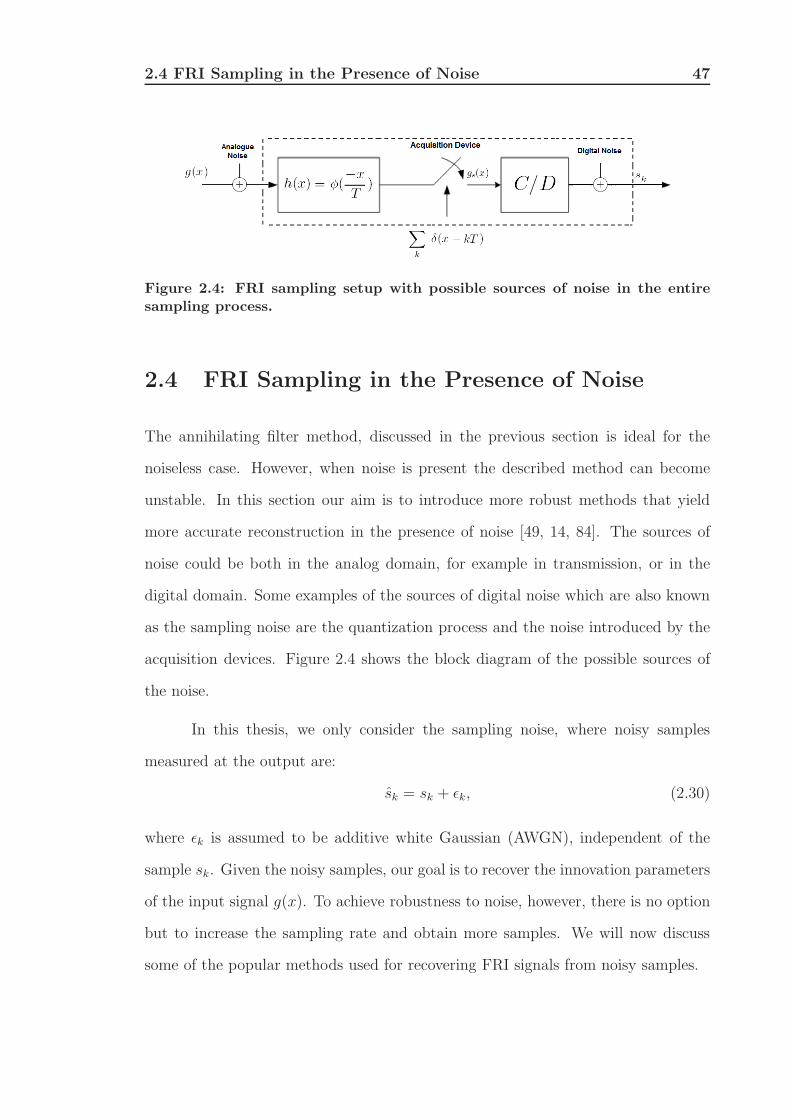
Figure 2.4: FRI sampling setup with possible sources of noise in the entiresampling process.
2.4 FRI Sampling in the Presence of Noise
The annihilating filter method, discussed in the previous section is ideal for the
noiseless case. However, when noise is present the described method can become
unstable. In this section our aim is to introduce more robust methods that yield
more accurate reconstruction in the presence of noise [49, 14, 84]. The sources of
noise could be both in the analog domain, for example in transmission, or in the
digital domain. Some examples of the sources of digital noise which are also known
as the sampling noise are the quantization process and the noise introduced by the
acquisition devices. Figure 2.4 shows the block diagram of the possible sources of
the noise.
In this thesis, we only consider the sampling noise, where noisy samples
measured at the output are:
sk = sk + ǫk, (2.30)
where ǫk is assumed to be additive white Gaussian (AWGN), independent of the
sample sk. Given the noisy samples, our goal is to recover the innovation parameters
of the input signal g(x). To achieve robustness to noise, however, there is no option
but to increase the sampling rate and obtain more samples. We will now discuss
some of the popular methods used for recovering FRI signals from noisy samples.

2.4 FRI Sampling in the Presence of Noise 48
2.4.1 Total Least-Squares Method
Given the noisy samples, the annihilating filter equation τ ·H = 0 will not be satisfied
exactly. However, as discussed in [14, 84, 59], a total least-squares approach can be
applied to reduce the effect of noise, by minimizing the Euclidean norm ||τ · H||2
under the constraint that ||H||2 = 1. This can be done by evaluating the singular-
value-decomposition (SVD) [55, 23] of the Toeplitz matrix τ = UΣVT , and choosing
the annihilating filter H to be the column vector of matrix V that corresponds to
the smallest singular value. As the matrix Σ is a diagonal matrix, containing the
singular value elements in a decreasing order, the last column vector of the matrix
V will correspond to the annihilating filter [14].
2.4.2 Matrix Pencil Method
Another popular subspace spectral estimation method is the matrix pencil method
[34, 35, 62] which makes use of Hankel matrices, singular-value-decomposition and
Eigen-value-decomposition (EVD) [55]. Matrix pencil method, tends to perform
well under noisy conditions and in our simulations it performs slightly better the
total least-squares method.
The estimation algorithm is as follows: As before, let us assume that we
have access to the measurements τm =∑K
k=1 ak umk , with unknown locations uk and
amplitudes ak. Then we arrange the measurements τm into a Hankel matrix H of
dimension M1 ×M2 as follows:
HM1×M2 =
τ0 τ1 . . . τM1−1
τ1 τ2 . . . τM1
......
. . ....
τM2−1 τM2−2 . . . τM1+M2−2
, (2.31)
2.4 FRI Sampling in the Presence of Noise 49
where M1 ≥ K + 1, M2 ≥ K. As for the annihilating filter method, the number
of measurements of τm should be at least 2K in order to fully recover the unknown
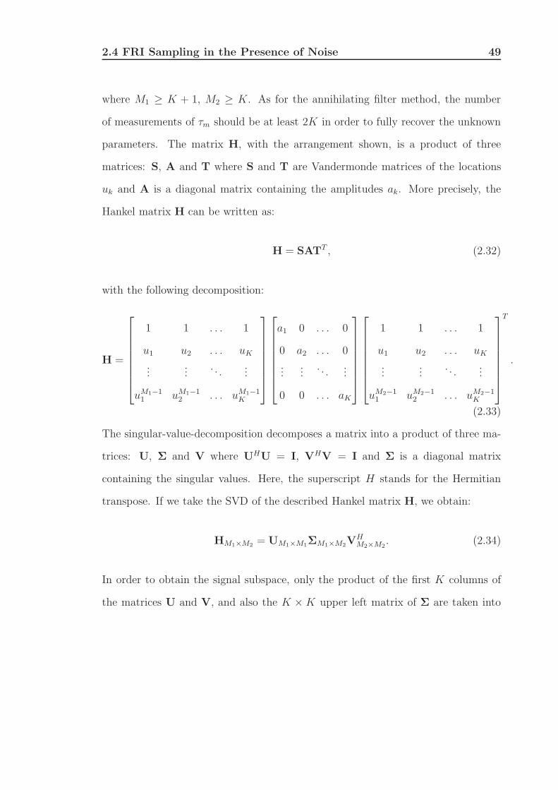
parameters. The matrix H, with the arrangement shown, is a product of three
matrices: S, A and T where S and T are Vandermonde matrices of the locations
uk and A is a diagonal matrix containing the amplitudes ak. More precisely, the
Hankel matrix H can be written as:
H = SATT , (2.32)
with the following decomposition:
H =
1 1 . . . 1
u1 u2 . . . uK...
.... . .
...
uM1−11 uM1−1
2 . . . uM1−1K
a1 0 . . . 0
0 a2 . . . 0
......
. . ....
0 0 . . . aK
1 1 . . . 1
u1 u2 . . . uK...
.... . .
...
uM2−11 uM2−1
2 . . . uM2−1K
T
.
(2.33)
The singular-value-decomposition decomposes a matrix into a product of three ma-
trices: U, Σ and V where UHU = I, VHV = I and Σ is a diagonal matrix
containing the singular values. Here, the superscript H stands for the Hermitian
transpose. If we take the SVD of the described Hankel matrix H, we obtain:
HM1×M2 = UM1×M1ΣM1×M2VHM2×M2
. (2.34)
In order to obtain the signal subspace, only the product of the first K columns of
the matrices U and V, and also the K ×K upper left matrix of Σ are taken into
2.4 FRI Sampling in the Presence of Noise 50
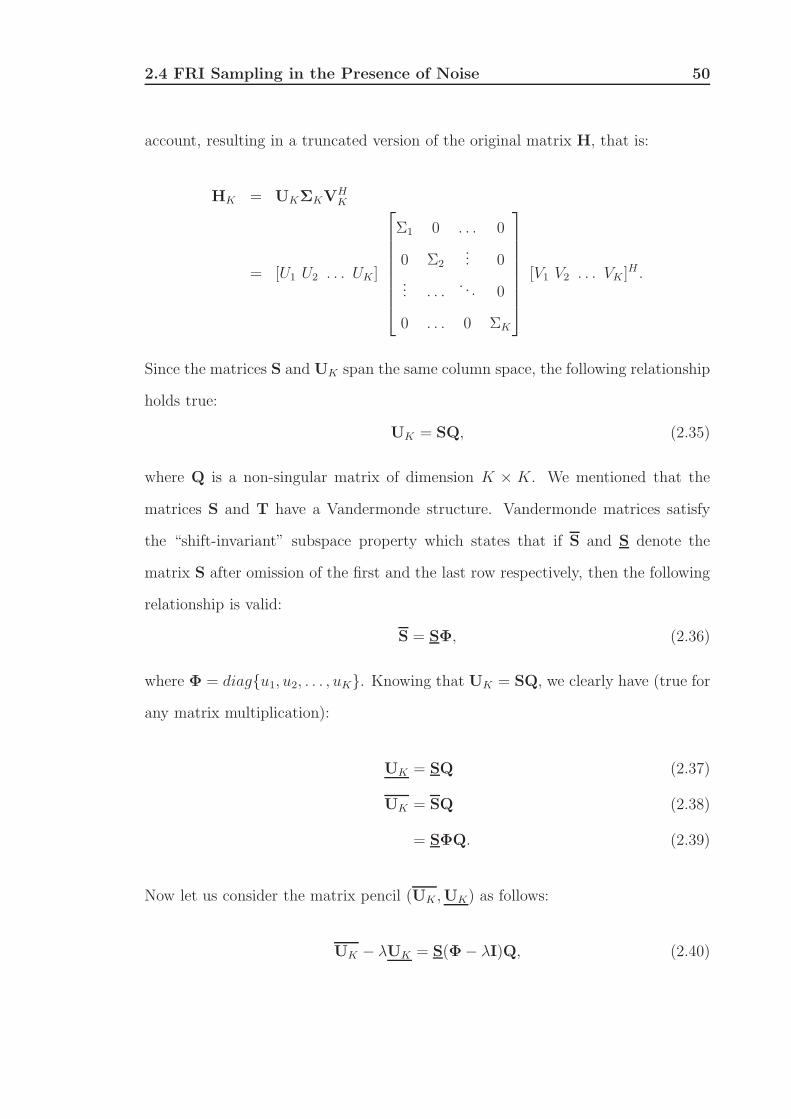
account, resulting in a truncated version of the original matrix H, that is:
HK = UKΣKVHK
= [U1 U2 . . . UK ]
Σ1 0 . . . 0
0 Σ2... 0
... . . .. . . 0
0 . . . 0 ΣK
[V1 V2 . . . VK ]H .
Since the matrices S and UK span the same column space, the following relationship
holds true:
UK = SQ, (2.35)
where Q is a non-singular matrix of dimension K × K. We mentioned that the
matrices S and T have a Vandermonde structure. Vandermonde matrices satisfy
the “shift-invariant” subspace property which states that if S and S denote the
matrix S after omission of the first and the last row respectively, then the following
relationship is valid:
S = SΦ, (2.36)
where Φ = diagu1, u2, . . . , uK. Knowing that UK = SQ, we clearly have (true for
any matrix multiplication):
UK = SQ (2.37)
UK = SQ (2.38)
= SΦQ. (2.39)
Now let us consider the matrix pencil (UK ,UK) as follows:
UK − λUK = S(Φ− λI)Q, (2.40)

2.4 FRI Sampling in the Presence of Noise 51
where λ is called the rank reducing number. We can solve for uk by finding the
Eigen-values of the matrix pencil. The problem of finding the Eigen-values of a
matrix pencil is called the “Generalized Eigen-value problem”. Therefore, to obtain
the locations uk we construct the following matrix equation:
UK−1.UK = Q−1ΦQ, (2.41)
where by taking the Eigen-value-decomposition, we obtain the matrix Φ which is a
diagonal matrix containing all the locations uk:
eig(UK−1UK) = eig(Q−1ΦQ) = Φ. (2.42)
Moreover, since we have found the exact values of the locations uk, we can now
construct the matrices S and T to obtain the amplitudes ak, using the following
equation:
A = (S†)H(TT )†, (2.43)
where the dagger † stands for pseudo-inverse of the matrix.
2.4.3 Cadzow’s Algorithm
The total least-squares method and the matrix pencil method are reliable only for
moderate values of noise. In [14], an iterative denoising algorithm, known as Cad-
zow’s algorithm [16, 72] is introduced where, when applied before one of the methods
discussed above, yields more robust and reliable results.
In the noiseless case, the Toeplitz matrix τ , which is constructed from the
measurements τm, has rank K, equal to the number of Diracs in the input signal.
This is due to the fact that the annihilating filter H in τ · H = 0, has K + 1
coefficients. When the signal is corrupted by noise, this rank deficiency property

2.5 Summary 52
is lost. However, by taking the SVD, we can assume that the K largest singular
values in τ = UΣVH correspond to the actual signal and the rest correspond to
the noise. To restore the rank deficiency property of the matrix, we set the singular
values of the noise to zero. This will in-turn alter the Toeplitz structure of the
original matrix, but by taking the average of the diagonals of the matrix, Toeplitz
structure can be restored back. By iterating this procedure, the matrix τ converges
to a well-approximated Toeplitz matrix of correct rank. The resulting matrix, is a
properly denoised version of the original matrix τ and the matrix pencil method or
the total-least squares method can be applied to the denoised matrix. Given a noise
contaminated discrete-time measurements of a signal, Cadzow’s algorithm exploits
the signal attributes (i.e. rank deficiency property and Toeplitz structure) from its
matrix representation.
The Cadzow’s algorithm combined with the matrix pencil method will be
utilized in the next chapter, when we consider the multichannel sampling of FRI
signal in the presence of noise.
2.5 Summary
In this chapter we presented a background on the 1-D sampling framework of FRI
signals. We described the different elements of the sampling setup and showed
how a set of 1-D Diracs can be sampled and perfectly reconstructed using both
polynomial and exponential reproducing kernels. Then we considered the case of
noisy measurements and presented some denoising techniques for the reconstruction
of the innovation parameters from the noisy samples.
53
Chapter 3
Multichannel Sampling of Finite
Rate of Innovation Signals
3.1 Introduction
Multichannel sampling was first proposed by Papoulis in the context of bandlim-
ited signals [58] in 1977. In his work, Papoulis introduced a powerful extension of
Shannon’s sampling theory, showing that a bandlimited signal g(x) could be recon-
structed exactly from the samples of M linear shift-invariant systems, sampled at
1/Mth of the Nyquist rate.
In this chapter we present a possible extension of the theory of sampling sig-
nals with finite rate of innovation to the case of multichannel acquisition systems.
The critical issue in our proposed multichannel sampling setup is the precise syn-
chronization of the various channels, since different devices introduce different drifts
and different gains within each channel. This could be due, for example, to imper-
fections of electronic circuits. For the signal reconstruction, these parameters need
to be estimated in advance, which we refer to as the channel synchronization stage.
In this chapter we consider the multichannel sampling of FRI signals and extend the
3.2 Multichannel Sampling Framework 54
results in [27] to this new scenario. The material of this chapter has been in part
published at [5].
The organization of this chapter is as follows: In the next section, we present
an extension of 1-D FRI sampling framework, discussed in the previous chapter,
to the case of multichannel sampling. In Section 3.3, by considering both the syn-
chronization stage and the signal reconstruction stage as a parametric estimation
problem, we propose our novel algorithm for multichannel sampling of FRI signals
and demonstrate that it is possible to simultaneously estimate the channel param-
eters (i.e., delays and gains) and the signal itself from the measured samples. This
is achieved by operating at a sampling rate proportional to 1/TM , where M is the
number of channels involved. In Section 3.5 we consider the noisy scenario and
assume that the samples are corrupted by additive white Gaussian noise. By eval-
uating the Cramer-Rao bounds and taking numerical simulations into account, we
asses the resilience to noise of multichannel sampling systems compared to single-
channel ones. We finally summarize this chapter in Section 3.6.
3.2 Multichannel Sampling Framework
3.2.1 Sampling Setup
Figure 3.1 shows our proposed multichannel setup for 1-D FRI signals. As shown
in the figure, the bank of acquisition devices or sampling kernels with functions
φ1(x), φ2(x), . . . , φM(x), receive drifted and scaled versions of the input FRI signal
g(x) denoted with ∆i and Ai for i = 2, 3, . . . ,M . Given the setup model, the prob-
lem can be divided into two stages, the channel synchronization stage and the signal
reconstruction stage. The samples si,k measured at the output of the multichannel
sampling setup are utilized jointly for the channel synchronization and the signal re-
3.2 Multichannel Sampling Framework 55
Figure 3.1: The proposed multichannel sampling setup for 1-D FRI signals.Here, the continuous-time signal g(x) is received by multiple channels withmultiple acquisition devices. The samples si,k from each channel are utilizedjointly for the reconstruction process.
construction process. Our goal is to see under what conditions the multiple channels
can be synchronized, that is under what conditions the estimation of the unknown
parameters ∆i and Ai is possible. Moreover, given the synchronized channels, we
also want to see under what conditions perfect reconstruction of the input FRI signal
g(x) can be achieved. In the following subsections all these questions are addressed
and a novel algorithm will be presented.
3.2.2 Sampling Kernels
For the multichannel setup shown in Figure 3.1, we will assume that the acquisition
devices are all E-spline sampling kernels. The reason for the use of such compact
support kernel is that, unlike polynomial reproducing kernels, dynamic multichan-
nel sampling is possible with E-splines. By dynamic sampling, we mean that the
overall number of samples required from the multichannel setup, can be arbitrarily
distributed within different channels, as long as the conditions necessary for channel
synchronization are met. This is due to the fact that, arbitrary exponentials can be
reproduced with E-splines and this rises from the arbitrary choice of the parameters
α0 and λ in αm = α0+mλ. Moreover, the exponents of the E-spline can be chosen so
3.3 Multichannel Sampling of Finite Rate of Innovation Signals 56
that a number of exponents are in common between the different sampling kernels
and this will allow the synchronization of the channels which will be explained in
detail in the next section.
3.3 Multichannel Sampling of Finite Rate of In-
novation Signals
3.3.1 Channel Synchronization
Without loss of generality, let us assume that the input signal g(x) is a stream of K
Diracs at distinct instants xk with amplitudes ak. Let us also assume for simplicity
that M = 2, that is, our multichannel system is restricted to two channels only. We
specify each channel sampling kernel to be of the form:
φ1(jω) =
P∏
m=0
(1− eαm−jω
jω − αm
)(3.1)
φ2(jω) =
Q∏
m=P−1
(1− eαm−jω
jω − αm
), (3.2)
where Q depends on the structure of the input signal. For simplicity we will assume
that Q = 2P − 1, so that both sampling kernels will be of equal order P + 1.
As can be seen from the equations given above, both kernels can reproduce the
exponentials eαP−1x and eαP x. Given our pre-specified sampling kernels, the input
signal is observed by each of the two channels and then sampled at a sampling
interval T . The samples sk of the i-th channel, where i = 1, 2 are thus given by:
si,k = 〈Aig(x−∆i), φi(x/T − k)〉, (3.3)
3.3 Multichannel Sampling of Finite Rate of Innovation Signals 57
where A1 = 1 and ∆1 = 0 within the first channel (or reference channel). Given
the samples, we calculate the exponential moments from the two channels, with the
proper coefficients c(i)m,k, i = 1, 2, as follows:
τ (1)m =N∑
k=0
c(1)m,ks1,k =
∫ ∞
−∞
g(x)eαmxdx, (3.4)
where m = 0, 1, . . . , P and,
τ (2)m =
N∑
k=0
c(2)m,ks2,k =
∫ ∞
−∞
A2g(x−∆2)eαmxdx = A2τ
(1)m eαm∆2 , (3.5)
where m = P − 1, P, . . . , 2P − 1. Here, the parameter N represents the number
of samples measured. As shown in the equations above, in our setup we have two
common parameters between the exponents of the two channels, that is atm = P−1
andm = P . Given these two common parameters, we can build the following system
of equations:
τ(2)P = A2τ
(1)P eαP∆2 (3.6)
τ(2)P−1 = A2τ
(1)P−1e
αP−1∆2 , (3.7)
Now, from the above equations, the delay and the gain parameters are estimated as
follows:
∆2 =1
αP−1 − αP
ln
(τ(1)P τ
(2)P−1
τ(1)P−1τ
(2)P
)(3.8)
and
A2 =τ(2)P
τ(1)P
e−αP∆2. (3.9)
Therefore with only two common parameters, the delay and gain parameters can be
estimated. We should point out that by having more than two common parameters,
more accurate estimations can be achieved for the unknown parameters, however,
one has to bear in mind that having more common parameters require higher spline
3.3 Multichannel Sampling of Finite Rate of Innovation Signals 58
orders for each channel and thus more samples will be needed.
From the set of results obtained above we can see that independently of the
input signal g(x), it is possible to synchronize the two channels exactly from the
samples si,k. However, a few considerations need to be addressed here. In the above
analysis we have implicitly assumed that τ(i)m 6= 0 for m = P − 1, P and i = 1, 2 and
this is not always true. Thus, for a guaranteed synchronization of the channels, some
constraints need to be imposed on the signal. In our context we are interested in
streams of Diracs and in this case the simple assumption that, given the K locations
of the Diracs, the amplitudes are drawn from a non-singular distribution over RK
guarantees that the event τ(i)m = 0 has probability zero. This is clearly a fairly mild
hypothesis and similar types of conditions can be imposed on any other FRI signal.
3.3.2 Signal Reconstruction
Let us now return to the original problem of reconstructing the stream of Diracs
g(x). Given the exact gain and delay of channel two, we can now estimate the
moments τ(1)m , with m = P + 1, P + 2, ..., 2P − 1 from τ
(2)m as follows:
τ (1)m =τ(2)m
A2e−αm∆2, m = P + 1, P + 2, ..., 2P − 1. (3.10)
It follows that if 2P −1 ≥ 2K−1 or, more simply, P ≥ K then a perfect recovery of
g(x) is possible from the moments τ(1)m , m = 0, 1, ...2P − 1 by using the annihilating
filter method discussed in Chapter 2. The advantage of the new setup is that we
now require splines of lower order (i.e., P ≥ K rather than P ≥ 2K − 1) and this
leads to shorter kernels.
For example, as mentioned in Chapter 2, the sampling of an infinite stream
of Diracs in the single-channel case requires that there are no more than K Diracs
3.3 Multichannel Sampling of Finite Rate of Innovation Signals 59
in an interval of size1 of 2K(P + 1)T ≤ 4K2T , where we have used the fact that
in the single-channel setup P ≥ 2K − 1. In the case of the two-channel acquisition
system, the interval is reduced to (2K2 + 2K)T since P ≥ K. This indicates that
in the new setup we can either sample signals with a higher concentration of Diracs
or alternatively for the same signal we can almost halve the sampling rate.
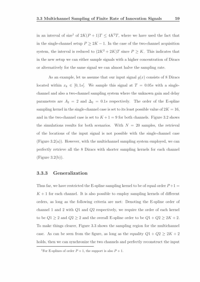
As an example, let us assume that our input signal g(x) consists of 8 Diracs
located within xk ∈ [0, 1s[. We sample this signal at T = 0.05s with a single-
channel and also a two-channel sampling system where the unknown gain and delay
parameters are A2 = 2 and ∆2 = 0.1s respectively. The order of the E-spline
sampling kernel in the single-channel case is set to its least possible value of 2K = 16,
and in the two-channel case is set to K +1 = 9 for both channels. Figure 3.2 shows
the simulations results for both scenarios. With N = 20 samples, the retrieval
of the locations of the input signal is not possible with the single-channel case
(Figure 3.2(a)). However, with the multichannel sampling system employed, we can
perfectly retrieve all the 8 Diracs with shorter sampling kernels for each channel
(Figure 3.2(b)).
3.3.3 Generalization
Thus far, we have restricted the E-spline sampling kernel to be of equal order P+1 =
K + 1 for each channel. It is also possible to employ sampling kernels of different
orders, as long as the following criteria are met: Denoting the E-spline order of
channel 1 and 2 with Q1 and Q2 respectively, we require the order of each kernel
to be Q1 ≥ 2 and Q2 ≥ 2 and the overall E-spline order to be Q1 + Q2 ≥ 2K + 2.
To make things clearer, Figure 3.3 shows the sampling region for the multichannel
case. As can be seen from the figure, as long as the equality Q1 + Q2 ≥ 2K + 2
holds, then we can synchronize the two channels and perfectly reconstruct the input
1For E-splines of order P + 1, the support is also P + 1.
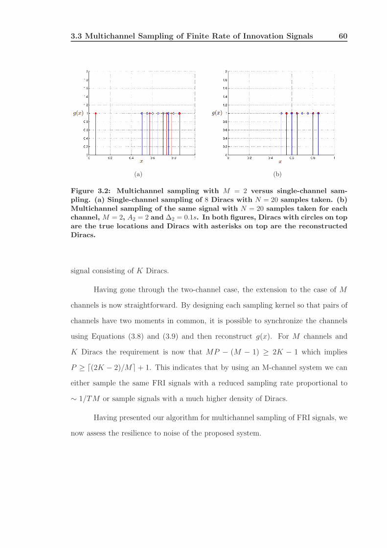
3.3 Multichannel Sampling of Finite Rate of Innovation Signals 60
(a) (b)
Figure 3.2: Multichannel sampling with M = 2 versus single-channel sam-pling. (a) Single-channel sampling of 8 Diracs with N = 20 samples taken. (b)Multichannel sampling of the same signal with N = 20 samples taken for eachchannel, M = 2, A2 = 2 and ∆2 = 0.1s. In both figures, Diracs with circles on topare the true locations and Diracs with asterisks on top are the reconstructedDiracs.
signal consisting of K Diracs.
Having gone through the two-channel case, the extension to the case of M
channels is now straightforward. By designing each sampling kernel so that pairs of
channels have two moments in common, it is possible to synchronize the channels
using Equations (3.8) and (3.9) and then reconstruct g(x). For M channels and
K Diracs the requirement is now that MP − (M − 1) ≥ 2K − 1 which implies
P ≥ ⌈(2K − 2)/M⌉ + 1. This indicates that by using an M-channel system we can
either sample the same FRI signals with a reduced sampling rate proportional to
∼ 1/TM or sample signals with a much higher density of Diracs.
Having presented our algorithm for multichannel sampling of FRI signals, we
now assess the resilience to noise of the proposed system.
3.4 Noisy Scenario 61
Figure 3.3: Multichannel sampling region with M = 2. Here, Q1 and Q2represent the E-spline sampling kernel order for each channel.
3.4 Noisy Scenario
We have seen already that, in the noiseless case, a multichannel acquisition system
achieves perfect reconstruction of FRI signals with a sampling rate proportional to
1/TM . Thus, perfect reconstruction is achieved at a sampling rate lower than the
single channel case. We now show both theoretically and numerically that, if we
do not reduce the sampling rate and leave it fixed at 1/T , a multichannel system
is more resilient to noise than a single-channel one. For numerical evaluation, we
will apply the denoising algorithms discussed in Chapter 2, particularly the matrix
pencil method and the Cadzow’s algorithm. For theoretical evaluation, we will use
a common and useful tool known as the Cramer-Rao bound which gives the lowest
achievable bound at a given noise level, for any unbiased estimator.
3.5 Multichannel Sampling of FRI Signals in the Presence of Noise 62
3.5 Multichannel Sampling of FRI Signals in the
Presence of Noise
Consider the multichannel sampling setup of Figure 3.1 and let us now assume that,
due to the noise, the samples we measure are given by:
si,k = 〈Aig(x−∆i), φi(x/T − k)〉+ ǫi,k, (3.11)
where k = 0, 1, ...N − 1, i = 1, 2, ...,M , ǫi,k is i.i.d. additive Gaussian noise with
zero mean and variance σ2 and T = L/N , with L = 1 seconds. We also assume
that the gains introduced by the channels are all equal and known a-priori, that is,
Ai = 1, i = 1, 2, ...,M , therefore only the delays need to be estimated. Moreover, we
assume that the input signal g(x) has K = 3 Diracs with known fixed amplitudes.
We have considered these assumptions only for the sake of simplicity, however, in
practice the gain parameters introduced and the amplitudes of the Diracs are not
necessarily known a-priori.
Our aim is to compare the performance of the single-channel setup (i.e.,
M = 1) against the two-channel and three-channel systems. Since for all cases
we have a standard parametric estimation problem, we use Cramer-Rao bounds
(CRB) to compare the minimum bounds of the different setups and probe whether
the multichannel systems are in theory more resilient to noise. The Cramer-Rao
bound is given by the inverse of the Fisher information (see Appendix A for full
derivation2):
CRB(Θ) = σ2
(N−1∑
k=0
∇f(Θ, k) · ∇f(Θ, k)T)−1
, (3.12)
2Regarding the single-channel case, we should point out that, Blu et al. [14] have computed theCramer-Rao bounds for sampling a single Dirac with a sinc kernel and Homann et al. [26] havecomputed the Cramer-Rao bounds for sampling a single Dirac with polynomial and exponentialreproducing kernels.
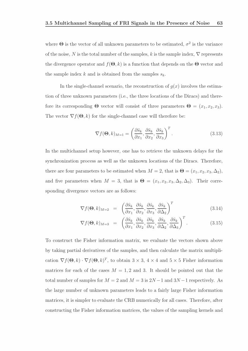
3.5 Multichannel Sampling of FRI Signals in the Presence of Noise 63
where Θ is the vector of all unknown parameters to be estimated, σ2 is the variance
of the noise, N is the total number of the samples, k is the sample index, ∇ represents
the divergence operator and f(Θ, k) is a function that depends on the Θ vector and
the sample index k and is obtained from the samples sk.
In the single-channel scenario, the reconstruction of g(x) involves the estima-
tion of three unknown parameters (i.e., the three locations of the Diracs) and there-
fore its corresponding Θ vector will consist of three parameters Θ = (x1, x2, x3).
The vector ∇f(Θ, k) for the single-channel case will therefore be:
∇f(Θ, k)M=1 =
(∂sk∂x1
,∂sk∂x2
,∂sk∂x3
)T
. (3.13)
In the multichannel setup however, one has to retrieve the unknown delays for the
synchronization process as well as the unknown locations of the Diracs. Therefore,
there are four parameters to be estimated when M = 2, that is Θ = (x1, x2, x3,∆2),
and five parameters when M = 3, that is Θ = (x1, x2, x3,∆2,∆3). Their corre-
sponding divergence vectors are as follows:
∇f(Θ, k)M=2 =
(∂sk∂x1
,∂sk∂x2
,∂sk∂x3
,∂sk∂∆2
)T
(3.14)
∇f(Θ, k)M=3 =
(∂sk∂x1
,∂sk∂x2
,∂sk∂x3
,∂sk∂∆2
,∂sk∂∆3
)T
. (3.15)
To construct the Fisher information matrix, we evaluate the vectors shown above
by taking partial derivatives of the samples, and then calculate the matrix multipli-
cation ∇f(Θ, k) · ∇f(Θ, k)T , to obtain 3 × 3, 4 × 4 and 5 × 5 Fisher information
matrices for each of the cases M = 1, 2 and 3. It should be pointed out that the
total number of samples forM = 2 andM = 3 is 2N−1 and 3N−1 respectively. As
the large number of unknown parameters leads to a fairly large Fisher information
matrices, it is simpler to evaluate the CRB numerically for all cases. Therefore, after
constructing the Fisher information matrices, the values of the sampling kernels and
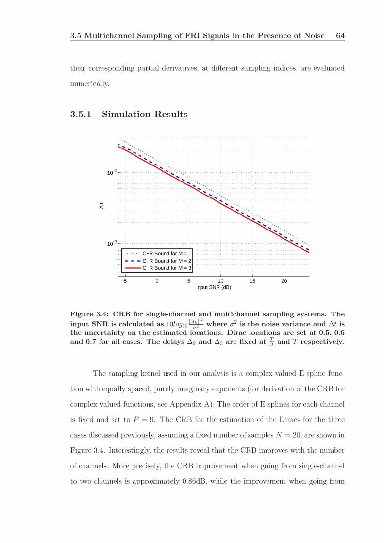
3.5 Multichannel Sampling of FRI Signals in the Presence of Noise 64
their corresponding partial derivatives, at different sampling indices, are evaluated
numerically.
3.5.1 Simulation Results
−5 0 5 10 15 20
10−3
10−2
Input SNR (dB)
∆ t
C−R Bound for M = 1C−R Bound for M = 2C−R Bound for M = 3
Figure 3.4: CRB for single-channel and multichannel sampling systems. The
input SNR is calculated as 10log10||sk||
2
σ2 where σ2 is the noise variance and ∆t isthe uncertainty on the estimated locations. Dirac locations are set at 0.5, 0.6and 0.7 for all cases. The delays ∆2 and ∆3 are fixed at T
2 and T respectively.
The sampling kernel used in our analysis is a complex-valued E-spline func-
tion with equally spaced, purely imaginary exponents (for derivation of the CRB for
complex-valued functions, see Appendix A). The order of E-splines for each channel
is fixed and set to P = 9. The CRB for the estimation of the Diracs for the three
cases discussed previously, assuming a fixed number of samples N = 20, are shown in
Figure 3.4. Interestingly, the results reveal that the CRB improves with the number
of channels. More precisely, the CRB improvement when going from single-channel
to two-channels is approximately 0.86dB, while the improvement when going from
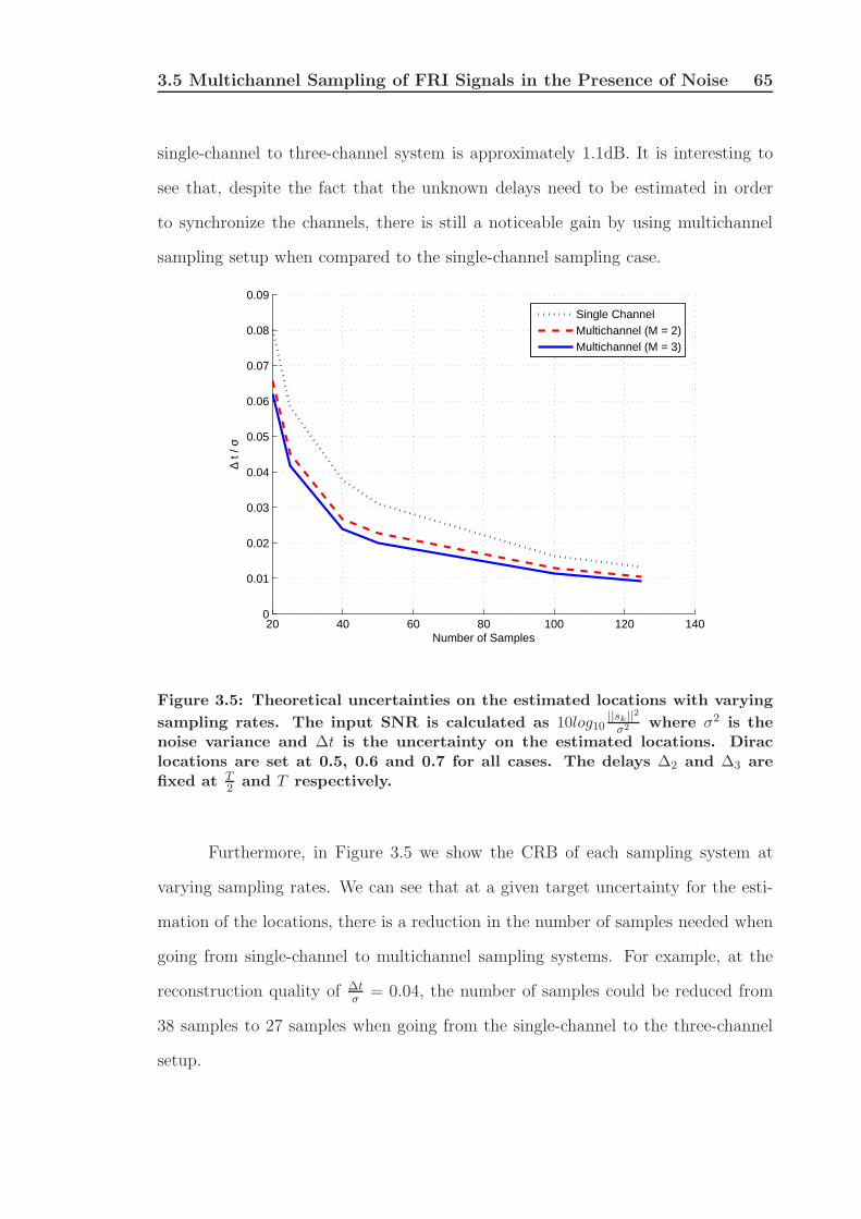
3.5 Multichannel Sampling of FRI Signals in the Presence of Noise 65
single-channel to three-channel system is approximately 1.1dB. It is interesting to
see that, despite the fact that the unknown delays need to be estimated in order
to synchronize the channels, there is still a noticeable gain by using multichannel
sampling setup when compared to the single-channel sampling case.
20 40 60 80 100 120 1400
0.01
0.02
0.03
0.04
0.05
0.06
0.07
0.08
0.09
Number of Samples
∆ t /
σ
Single ChannelMultichannel (M = 2)Multichannel (M = 3)
Figure 3.5: Theoretical uncertainties on the estimated locations with varying
sampling rates. The input SNR is calculated as 10log10||sk||
2
σ2 where σ2 is thenoise variance and ∆t is the uncertainty on the estimated locations. Diraclocations are set at 0.5, 0.6 and 0.7 for all cases. The delays ∆2 and ∆3 arefixed at T
2 and T respectively.
Furthermore, in Figure 3.5 we show the CRB of each sampling system at
varying sampling rates. We can see that at a given target uncertainty for the esti-
mation of the locations, there is a reduction in the number of samples needed when
going from single-channel to multichannel sampling systems. For example, at the
reconstruction quality of ∆tσ
= 0.04, the number of samples could be reduced from
38 samples to 27 samples when going from the single-channel to the three-channel
setup.
3.5 Multichannel Sampling of FRI Signals in the Presence of Noise 66
−10 0 10 20 30 40 5010
−5
10−4
10−3
10−2
10−1
100
Input SNR (dB)
∆ t
RMS Error for M = 1C−R Bound for M = 1RMS Error for M = 2C−R Bound for M = 2RMS Error for M = 3C−R Bound for M = 3
Figure 3.6: Numerical results with single and multichannel sampling. The
input SNR is calculated as 10log10||sk||
2
σ2 where σ2 is the noise variance and ∆t isthe uncertainty on the estimated locations. Dirac locations are set at 0.5, 0.6and 0.7 for all cases. The delays ∆2 and ∆3 are fixed at T
2 and T respectively.
To analyse the performance of the reconstruction algorithm, Figure 3.6
presents some actual numerical results on the uncertainty of the estimated loca-
tions which are also compared against the theoretical bounds from Figure 3.4. The
delays are estimated using Equation (3.8), while the locations of the Diracs are
obtained using the matrix pencil method and also the Cadzow’s algorithm to fur-
ther denoise the exponential moments τm. While none of the algorithms achieve the
CRB, our results show that the gain in performance with multichannel sampling over
single-channel sampling can be significant. For instance, at input SNR= 15dB, the
gain in performance from single-channel to three-channels is approximately 4.4dB.
The additional noise robustness in our numerical simulations when compared to the
CRB is mostly due to the denoising algorithms that we use. This will be further
discussed in our ’Future Research’ section in Chapter 6.

3.6 Summary 67
3.6 Summary
In this chapter we have extended the theory of sampling FRI signals to the case
of multichannel acquisition systems. We illustrated that by synchronizing the dif-
ferent channels of the proposed multichannel sampling setup, one can estimate the
unknown delays and gains introduced within the channels, regardless of the input
FRI signal. In the case of noisy measurements, we showed that by evaluating the
CRB, the multichannel system can achieve a target performance with a number of
samples which is smaller than the number of samples needed in the single-channel
setup. The improvement in the resilience to noise of the multi-channel architecture
was also confirmed with numerical simulations.

69
Chapter 4
System Identification based on the
Theories of Finite Rate of
Innovation Sampling
4.1 Introduction
In many practical applications the impulse response of an unknown system is re-
quired to be estimated. This problem which is usually referred to as “System Iden-
tification Problem” in literature has a vast number of applications, such as line
echo cancellation, channel equalization and model mismatch estimation. Figure 4.1
shows a system identification problem setup where a signal g(x) is fed to an unknown
system with impulse response ψ(x). The output signal from the unknown system
then goes through a sampling process with a sampling rate 1/T which outputs the
samples sk.
The aim of system identification is to completely determine the function ψ(x)
from the samples sk. Unlike standard techniques for system identification, such as
least mean squares (LMS) algorithm [63], which require the sampling rate to be at
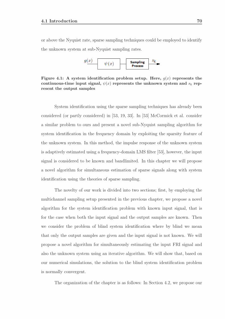
4.1 Introduction 70
or above the Nyquist rate, sparse sampling techniques could be employed to identify
the unknown system at sub-Nyquist sampling rates.
Figure 4.1: A system identification problem setup. Here, g(x) represents thecontinuous-time input signal, ψ(x) represents the unknown system and sk rep-resent the output samples
System identification using the sparse sampling techniques has already been
considered (or partly considered) in [53, 19, 33]. In [53] McCormick et al. consider
a similar problem to ours and present a novel sub-Nyquist sampling algorithm for
system identification in the frequency domain by exploiting the sparsity feature of
the unknown system. In this method, the impulse response of the unknown system
is adaptively estimated using a frequency-domain LMS filter [53], however, the input
signal is considered to be known and bandlimited. In this chapter we will propose
a novel algorithm for simultaneous estimation of sparse signals along with system
identification using the theories of sparse sampling.
The novelty of our work is divided into two sections; first, by employing the
multichannel sampling setup presented in the previous chapter, we propose a novel
algorithm for the system identification problem with known input signal, that is
for the case when both the input signal and the output samples are known. Then
we consider the problem of blind system identification where by blind we mean
that only the output samples are given and the input signal is not known. We will
propose a novel algorithm for simultaneously estimating the input FRI signal and
also the unknown system using an iterative algorithm. We will show that, based on
our numerical simulations, the solution to the blind system identification problem
is normally convergent.
The organization of the chapter is as follows: In Section 4.2, we propose our
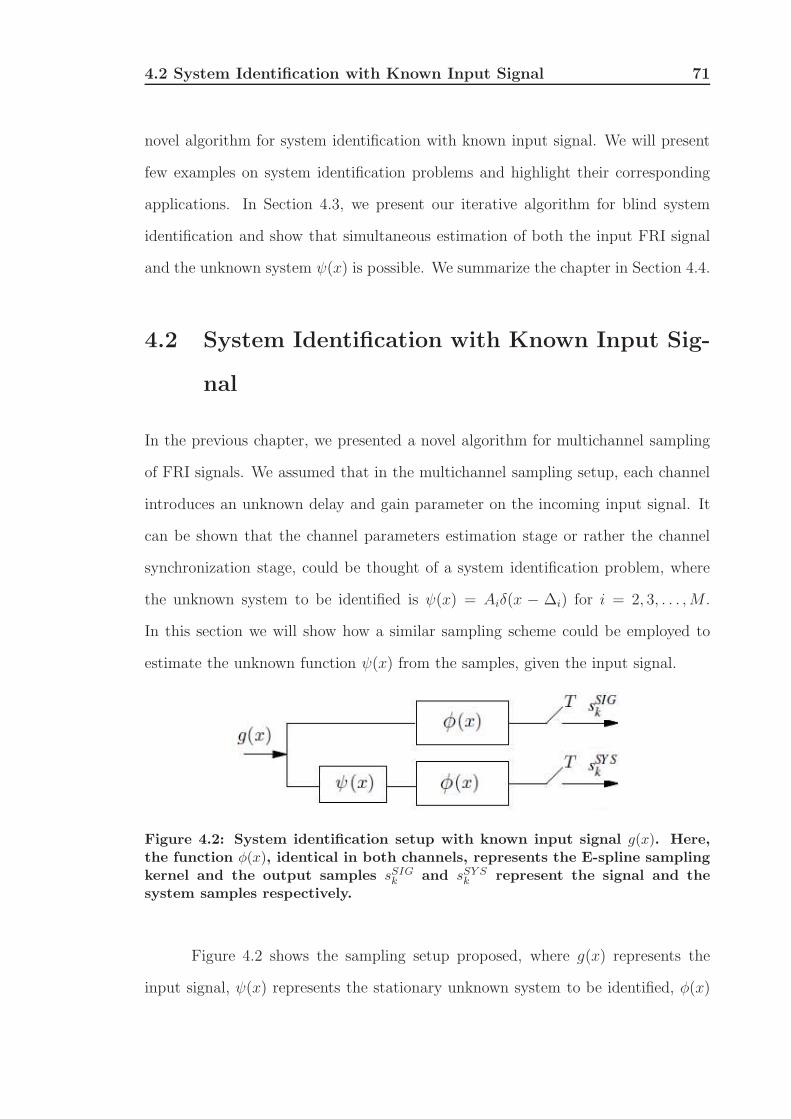
4.2 System Identification with Known Input Signal 71
novel algorithm for system identification with known input signal. We will present
few examples on system identification problems and highlight their corresponding
applications. In Section 4.3, we present our iterative algorithm for blind system
identification and show that simultaneous estimation of both the input FRI signal
and the unknown system ψ(x) is possible. We summarize the chapter in Section 4.4.
4.2 System Identification with Known Input Sig-
nal
In the previous chapter, we presented a novel algorithm for multichannel sampling
of FRI signals. We assumed that in the multichannel sampling setup, each channel
introduces an unknown delay and gain parameter on the incoming input signal. It
can be shown that the channel parameters estimation stage or rather the channel
synchronization stage, could be thought of a system identification problem, where
the unknown system to be identified is ψ(x) = Aiδ(x − ∆i) for i = 2, 3, . . . ,M .
In this section we will show how a similar sampling scheme could be employed to
estimate the unknown function ψ(x) from the samples, given the input signal.
Figure 4.2: System identification setup with known input signal g(x). Here,the function φ(x), identical in both channels, represents the E-spline samplingkernel and the output samples sSIGk and sSY S
k represent the signal and thesystem samples respectively.
Figure 4.2 shows the sampling setup proposed, where g(x) represents the
input signal, ψ(x) represents the stationary unknown system to be identified, φ(x)
4.2 System Identification with Known Input Signal 72
represents the sampling kernel which is considered to be an E-spline and sk represent
the samples. As can be seen, a two-channel sampling system with identical sampling
kernels has been employed to sample the input signal with and without the unknown
system ψ(x). In the first channel, the input signal is directly sampled with our pre-
specified E-spline sampling kernel φ(x). We recall here that the Fourier transform
of φ(x) is given by:
φ(jω) =
P∏
m=0
(1− eαm−jω
jω − αm
), (4.1)
where P depends only on the structure of the unknown function ψ(x). This will
be more evident later on. The samples sk at the output of the first channel are
therefore:
sSIGk = 〈g(x), φ(x− k)〉. (4.2)
Given the samples, we then calculate the exponential moments of the input signal,
as was shown in Equation (2.20). For the sake of clarity and without loss of gener-
ality, we will assume that the αm parameters are purely imaginary αm = jmλ and
therefore:
τSIGm = g(αm), (4.3)
where g(αm) represents the Fourier transform of the signal g(x) at αm with m =
0, 1, . . . , P . In the second channel, the same input signal is fed through the unknown
function ψ(x) and then sampled with the same sampling kernel. Therefore, its
corresponding samples sk are:
sSY Sk = 〈g(x) ∗ ψ(x), φ(x− k)〉. (4.4)
Given the samples of the second channel, we calculate its corresponding exponential
moments. This will lead to:
τSY Sm = g(αm) · ψ(αm). (4.5)
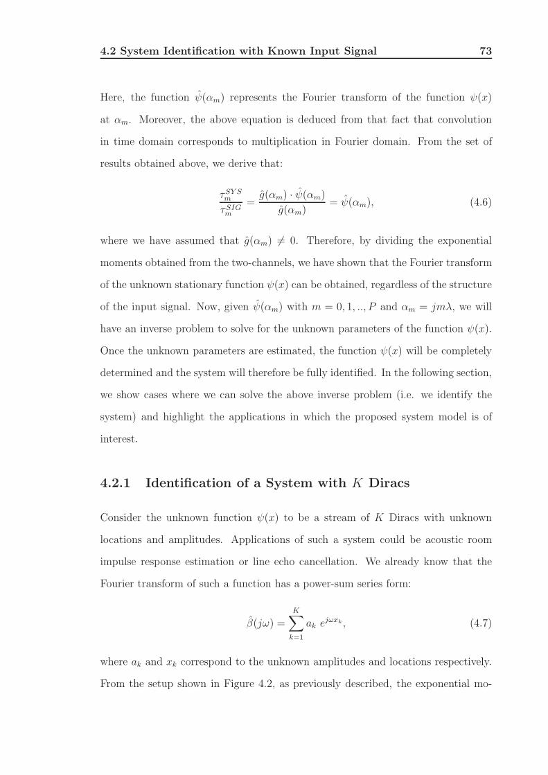
4.2 System Identification with Known Input Signal 73
Here, the function ψ(αm) represents the Fourier transform of the function ψ(x)
at αm. Moreover, the above equation is deduced from that fact that convolution
in time domain corresponds to multiplication in Fourier domain. From the set of
results obtained above, we derive that:
τSY Sm
τSIGm
=g(αm) · ψ(αm)
g(αm)= ψ(αm), (4.6)
where we have assumed that g(αm) 6= 0. Therefore, by dividing the exponential
moments obtained from the two-channels, we have shown that the Fourier transform
of the unknown stationary function ψ(x) can be obtained, regardless of the structure
of the input signal. Now, given ψ(αm) with m = 0, 1, .., P and αm = jmλ, we will
have an inverse problem to solve for the unknown parameters of the function ψ(x).
Once the unknown parameters are estimated, the function ψ(x) will be completely
determined and the system will therefore be fully identified. In the following section,
we show cases where we can solve the above inverse problem (i.e. we identify the
system) and highlight the applications in which the proposed system model is of
interest.
4.2.1 Identification of a System with K Diracs
Consider the unknown function ψ(x) to be a stream of K Diracs with unknown
locations and amplitudes. Applications of such a system could be acoustic room
impulse response estimation or line echo cancellation. We already know that the
Fourier transform of such a function has a power-sum series form:
β(jω) =K∑
k=1
ak ejωxk , (4.7)
where ak and xk correspond to the unknown amplitudes and locations respectively.
From the setup shown in Figure 4.2, as previously described, the exponential mo-
4.2 System Identification with Known Input Signal 74
ments of the output samples with and without the unknown function, that is τSY Sm
and τSIGm are obtained. The Fourier transform of the function ψ(x) at αm = jmλ
can now be easily calculated as follows:
τSY Sm
τSIGm
= ψ(αm), (4.8)
where,
ψ(αm) = β(αm) (4.9)
=
K∑
k=1
akeαmxk (4.10)
=K∑
k=1
akumk , m = 0, 1, . . . , P, (4.11)
where uk = ejλxk . As ψ(αm) has a power-sum series form, we apply the annihilating
filter method to the measurements τSY Sm
τSIGm
= ψ(αm) to retrieve the unknown param-
eters ak and xk. For such a system, in order to recover the K Diracs, the E-spline
sampling kernel is required to be of order P ≥ 2K. This setup is similar to the one
discussed in [33].
As an example, let us assume that our signal g(x) is a piecewise-polynomial
signal and the unknown function ψ(x) is a stream of 3 Diracs. Our goal is to
estimate the system, given the input signal and its corresponding sSIGk and sSY Sk
samples. Figure 4.3 shows the simulation results for this example. We can see that
the unknown system is perfectly estimated, regardless of the structure of the input
signal.
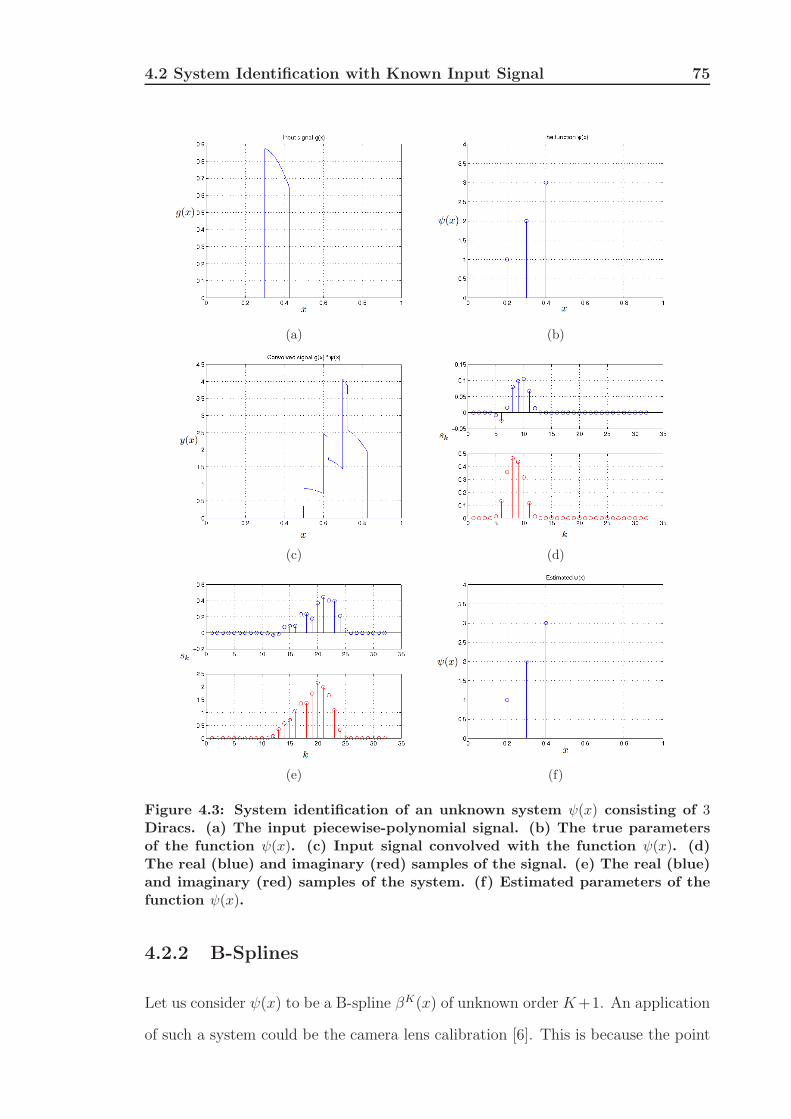
4.2 System Identification with Known Input Signal 75
(a) (b)
(c) (d)
(e) (f)
Figure 4.3: System identification of an unknown system ψ(x) consisting of 3Diracs. (a) The input piecewise-polynomial signal. (b) The true parametersof the function ψ(x). (c) Input signal convolved with the function ψ(x). (d)The real (blue) and imaginary (red) samples of the signal. (e) The real (blue)and imaginary (red) samples of the system. (f) Estimated parameters of thefunction ψ(x).
4.2.2 B-Splines
Let us consider ψ(x) to be a B-spline βK(x) of unknown order K+1. An application
of such a system could be the camera lens calibration [6]. This is because the point
4.2 System Identification with Known Input Signal 76
spread function of a camera lens is very often assumed to be a Gaussian pulse and
B-splines of order K ≥ 2 are increasingly similar to Gaussian functions. We already
know that the Fourier transform function of a B-spline of order K + 1 is given by:
βK(jω) =
K∏
k=0
1− e−jω
jω=
(1− e−jω
jω
)K+1
. (4.12)
Assuming the unknown function in our setup shown in Figure 4.2 is a B-spline of
unknown order, that is ψ(x) = βK(x), then by calculating the exponential moments
of the output samples with and without the unknown filter, we can obtain the
Fourier transform of ψ(x) at αm = jmλ as follows:
τSY Sm
τSIGm
= ψ(αm), (4.13)
where,
ψ(αm) = βK(αm) (4.14)
=
(1− e−αm
αm
)K+1
. (4.15)
By taking logarithms on both sides of the equation, the unknown order K + 1 is
calculated as follows:log(ψ(αm)
)
log(
1−e−αm
αm
) = K + 1. (4.16)
In order to estimate the unknown order of the B-spline, the E-spline sampling kernel
is required to be of order P ≥ 1.
As an example, let us assume that our signal g(x) consists of 2 Diracs and
the unknown function ψ(x) to be estimated is a B-spline of order 4. Our goal is to
estimate the order of the B-spline, given the input signal and its corresponding sSIGk
and sSY Sk samples. Figure 4.4 shows the simulation results for this example. As
can be seen from the figure, the system with B-spline of order 4 has been perfectly
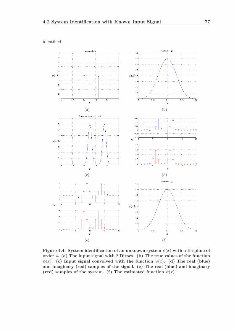
4.2 System Identification with Known Input Signal 77
identified.
(a) (b)
(c) (d)
(e) (f)
Figure 4.4: System identification of an unknown system ψ(x) with a B-spline oforder 4. (a) The input signal with 2 Diracs. (b) The true values of the functionψ(x). (c) Input signal convolved with the function ψ(x). (d) The real (blue)and imaginary (red) samples of the signal. (e) The real (blue) and imaginary(red) samples of the system. (f) The estimated function ψ(x).
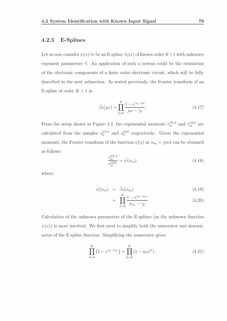
4.2 System Identification with Known Input Signal 78
4.2.3 E-Splines
Let us now consider ψ(x) to be an E-spline β~γ(x) of known orderK+1 with unknown
exponent parameters ~γ. An application of such a system could be the estimation
of the electronic components of a finite order electronic circuit, which will be fully
described in the next subsection. As stated previously, the Fourier transform of an
E-spline of order K + 1 is:
β~γ(jω) =
K∏
k=0
1− eγk−jω
jω − γk. (4.17)
From the setup shown in Figure 4.2, the exponential moments τSY Sm and τSIGm are
calculated from the samples sSY Sk and sSIGk respectively. Given the exponential
moments, the Fourier transform of the function ψ(x) at αm = jmλ can be obtained
as follows:
τSY Sm
τSIGm
= ψ(αm), (4.18)
where,
ψ(αm) = β~γ(αm) (4.19)
=K∏
k=0
1− eγk−αm
αm − γk. (4.20)
Calculation of the unknown parameters of the E-splines (as the unknown function
ψ(x)) is more involved. We first need to simplify both the numerator and denomi-
nator of the E-spline function. Simplifying the numerator gives:
K∏
k=0
(1− eγk−αm
)=
K∏
k=0
(1− akum) , (4.21)
4.2 System Identification with Known Input Signal 79
where ak = eγk and um = eαm . This can be further simplified as follows:
K∏
k=0
(1− akum) = (1− a1u
m)(1− a2um)...(1− aKu
m) (4.22)
=
K∑
k=0
qkukm (4.23)
=
K∑
k=0
qktmk , (4.24)
where tk = uk. Simplifying the denominator gives:
K∏
k=0
(αm − γk) = Q(m) =
K∑
k=0
rkmk, (4.25)
where Q(m) is a polynomial of degree K + 1. Rearranging Equation (4.20) using
Equation (4.24) and (4.25), leads to:
K∑
k=0
rkmk · ψ(αm) =
K∑
k=0
qktmk . (4.26)
The above equation can be considered as a linear system, consisting of 2K unknowns
with the unknown parameters being Θ = (r0, r1, . . . , rK−1, q1, . . . , qK). Here, q0 = 1,
t0 = 1 and tk are a known set of parameters. As we have a linear system, by
constructing the following matrix equation and taking its inverse we are able to
calculate the unknown parameters:
ψ(α0) 0 . . . 0 1 . . . 1
ψ(α1) ψ(α1) . . . ψ(α1) t2 . . . tK
ψ(α2) 2ψ(α2) . . . 2K−1ψ(α2) t22
. . . t2K
... . . . . . . . . . . . . . . ....
ψ(α2K−1) (2K − 1)ψ(α2K−1) . . . (2K − 1)K−1ψ(α2K−1) t2K−1
2. . . t2K−1
K
4.2 System Identification with Known Input Signal 80
×
r0
r1...
rK−1
q1...
qK
=
1
1− ψ(α1)rK
1− 2Kψ(α2)rK...
1− (2K − 1)Kψ(α2K−1)rK
. (4.27)
Once the parameters are estimated, by taking the roots of the polynomial qk for
k = 0, 1, . . . , K and then taking the logarithm of the roots we obtain the unknown
γk parameters, since roots(qk) = ak = eγk . The E-spline sampling kernel is required
to be of order P ≥ 2K in order to estimate the parameters of the E-spline function
ψ(x).
As an example, let us assume that our input signal g(x) consists of 2 Diracs
and the unknown function ψ(x) to be estimated is an E-spline of order 2 with
γ0 = −1 and γ1 = 2. Our goal is to estimate the system, given the input signal and
its corresponding sSIGk and sSY Sk samples. Figure 4.5 shows the simulation results
for this example. As can be seen from the figure, the function ψ(x) is fully identified
(The small error is due to numerical imprecision).
4.2.4 Linear Time-Invariant Circuits
Finite order linear time-invariant electronic circuits can be modelled as modified
E-splines [27]. In general any p-th order electronic circuit has a transfer function
(s = jω):
β(s) =bqs
q + bq−1sq−1 + . . .+ b1q + b0
apsp + ap−1sp−1 + . . .+ a1p+ a0=
∑Q
q=0 bqsq
∑P
p=0 apsp. (4.28)
The equation above has a very similar structure to the E-spline case and one may
suggest a similar simplifying procedure with constructing a system of linear equa-
tions with Q + P + 1 unknowns, as discussed previously. However, the transient
response of a finite order electronic circuit is infinite and this would mean that the
function ψ(x) will not be time-limited. Assuming that the electronic circuit has a
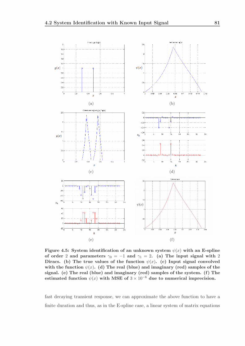
4.2 System Identification with Known Input Signal 81
(a) (b)
(c) (d)
(e) (f)
Figure 4.5: System identification of an unknown system ψ(x) with an E-splineof order 2 and parameters γ0 = −1 and γ1 = 2. (a) The input signal with 2Diracs. (b) The true values of the function ψ(x). (c) Input signal convolvedwith the function ψ(x). (d) The real (blue) and imaginary (red) samples of thesignal. (e) The real (blue) and imaginary (red) samples of the system. (f) Theestimated function ψ(x) with MSE of 3× 10⁻⁶ due to numerical imprecision.
fast decaying transient response, we can approximate the above function to have a
finite duration and thus, as in the E-spline case, a linear system of matrix equations
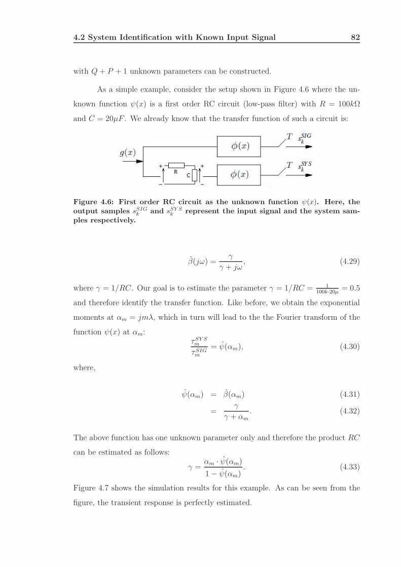
4.2 System Identification with Known Input Signal 82
with Q+ P + 1 unknown parameters can be constructed.
As a simple example, consider the setup shown in Figure 4.6 where the un-
known function ψ(x) is a first order RC circuit (low-pass filter) with R = 100kΩ
and C = 20µF . We already know that the transfer function of such a circuit is:
Figure 4.6: First order RC circuit as the unknown function ψ(x). Here, theoutput samples sSIGk and sSY S
k represent the input signal and the system sam-ples respectively.
β(jω) =γ
γ + jω, (4.29)
where γ = 1/RC. Our goal is to estimate the parameter γ = 1/RC = 1100k·20µ
= 0.5
and therefore identify the transfer function. Like before, we obtain the exponential
moments at αm = jmλ, which in turn will lead to the the Fourier transform of the
function ψ(x) at αm:τSY Sm
τSIGm
= ψ(αm), (4.30)
where,
ψ(αm) = β(αm) (4.31)
=γ
γ + αm
. (4.32)
The above function has one unknown parameter only and therefore the product RC
can be estimated as follows:
γ =αm · ψ(αm)
1− ψ(αm). (4.33)
Figure 4.7 shows the simulation results for this example. As can be seen from the
figure, the transient response is perfectly estimated.
4.3 Blind System Identification 83
We have shown in this section that by having access to the input signal and by
exploiting the sparsity feature of the unknown system, system identification problem
can be solved at low sampling rates by employing a multichannel sampling setup.
Sampling at lower rates, which generally results in the reduction of computational
complexity, is indeed the main advantage of our proposed algorithm when compared
to the classical methods. The amount of complexity reduction and other features
such as accuracy and noise robustness of our proposed method is an area of future
research and currently is out of the scope of our work.
4.3 Blind System Identification
In the previous section, we looked at the case where both the input signal and the
output samples were known. For the case of blind system identification however,
that is when both the input signal and the system are unknown, the above solution
cannot be used directly and the problem is more involved. However, a recursive
version of the previously discussed method, as shown in Figure 4.8(a) and 4.8(b),
can be utilized to estimate both the input FRI signal and the unknown function
ψ(x). Let us assume that the input sparse signal is a stream of Diracs with unknown
locations. As shown in Figure 4.8(a), the unknown input signal is fed to the unknown
system ψ(x) and then is sampled with our pre-specified E-spline sampling kernel with
αm = jmλ. Therefore, its corresponding exponential moments are:
τ 0m = ψ(αm) · g(αm), (4.34)
where both ψ(αm) and g(αm) are unknown. As our input signal is a stream of
Diracs with unknown locations, we directly apply the annihilating filter method
to the moments τ 0m and obtain an estimate of the input signal, denoted as g(x)
(Figure 4.8(b)). Once an estimate of the input signal is obtained, we recursively
feed the estimated signal g(x) back to our pre-specified sampling kernel and obtain
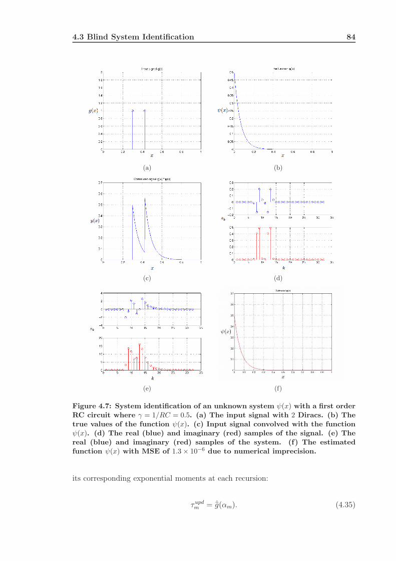
4.3 Blind System Identification 84
(a) (b)
(c) (d)
(e) (f)
Figure 4.7: System identification of an unknown system ψ(x) with a first orderRC circuit where γ = 1/RC = 0.5. (a) The input signal with 2 Diracs. (b) Thetrue values of the function ψ(x). (c) Input signal convolved with the functionψ(x). (d) The real (blue) and imaginary (red) samples of the signal. (e) Thereal (blue) and imaginary (red) samples of the system. (f) The estimatedfunction ψ(x) with MSE of 1.3× 10⁻⁶ due to numerical imprecision.
its corresponding exponential moments at each recursion:
τupdm = ˆg(αm). (4.35)
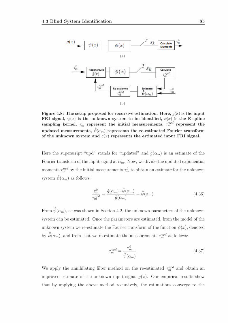
4.3 Blind System Identification 85
(a)
(b)
Figure 4.8: The setup proposed for recursive estimation. Here, g(x) is the inputFRI signal, ψ(x) is the unknown system to be identified, φ(x) is the E-spline
sampling kernel, τ0m represent the initial measurements, τupdm represent the
updated measurements,ˆψ(αm) represents the re-estimated Fourier transform
of the unknown system and g(x) represents the estimated input FRI signal.
Here the superscript “upd” stands for “updated” and ˆg(αm) is an estimate of the
Fourier transform of the input signal at αm. Now, we divide the updated exponential
moments τupdm by the initial measurements τ 0m to obtain an estimate for the unknown
system ψ(αm) as follows:
τ 0m
τupdm
=g(αm) · ψ(αm)
ˆg(αm)= ˆψ(αm). (4.36)
From ˆψ(αm), as was shown in Section 4.2, the unknown parameters of the unknown
system can be estimated. Once the parameters are estimated, from the model of the
unknown system we re-estimate the Fourier transform of the function ψ(x), denoted
byˆψ(αm), and from that we re-estimate the measurements τupdm as follows:
τupdm =τ 0m
ˆψ(αm)
. (4.37)
We apply the annihilating filter method on the re-estimated τupdm and obtain an
improved estimate of the unknown input signal g(x). Our empirical results show
that by applying the above method recursively, the estimations converge to the
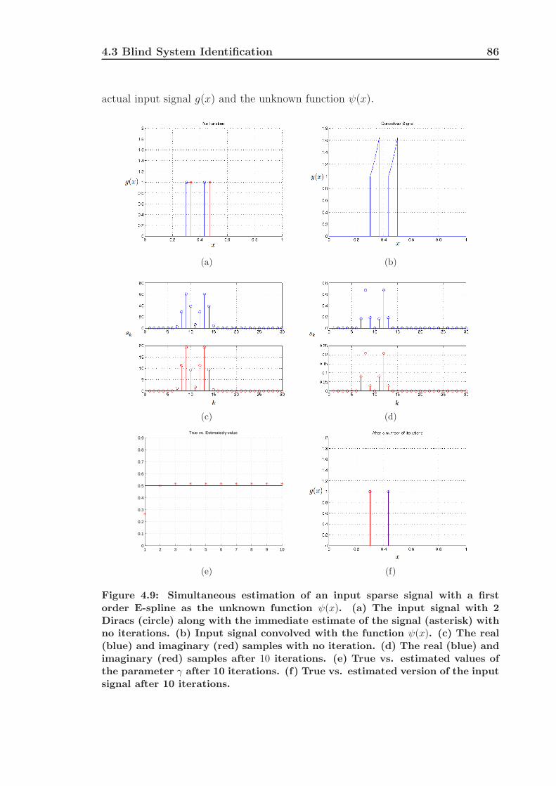
4.3 Blind System Identification 86
actual input signal g(x) and the unknown function ψ(x).
(a) (b)
(c) (d)
1 2 3 4 5 6 7 8 9 100
0.1
0.2
0.3
0.4
0.5
0.6
0.7
0.8
0.9True vs. Estimated γ value
(e) (f)
Figure 4.9: Simultaneous estimation of an input sparse signal with a firstorder E-spline as the unknown function ψ(x). (a) The input signal with 2Diracs (circle) along with the immediate estimate of the signal (asterisk) withno iterations. (b) Input signal convolved with the function ψ(x). (c) The real(blue) and imaginary (red) samples with no iteration. (d) The real (blue) andimaginary (red) samples after 10 iterations. (e) True vs. estimated values ofthe parameter γ after 10 iterations. (f) True vs. estimated version of the inputsignal after 10 iterations.
4.4 Summary 87
As an example let us assume that our input signal consists of 2 Diracs with
unknown location. Let us also assume that the unknown system to be identified is
a first order E-spline with γ = 2. Our goal is to simultaneously estimate the input
signal and also the unknown γ parameter. Figure 4.9 shows the results for the above
example after 10 iterations. It can be seen that both the input signal and also the
unknown system are estimated to a very good degree when compared to their true
values.
As another example, let us consider the unknown system to be identified to
be a first order RC circuit with γ = 1/RC = 2 where R = 100kΩ and C = 5µF .
Figure 4.9 shows the results for the above example after 20 iterations. It can be
seen that both the input signal and also the unknown system are estimated to a
very good degree when compared to their true values.
4.4 Summary
In this chapter we proposed our novel algorithms for system identification prob-
lem, based on the finite rate of innovation sampling theories. The novelty of this
chapter was divided into two section, where in the first section, we showed that by
having access to the input signal, system identification problem could be solved at
low sampling rates by employing the multichannel sampling setup and exponential
moments. Then, in the second section, we considered the problem of blind system
identification. We showed that a recursive method could be utilized to estimate
both the input FRI signal and also the unknown system when we only have access
to the output samples.
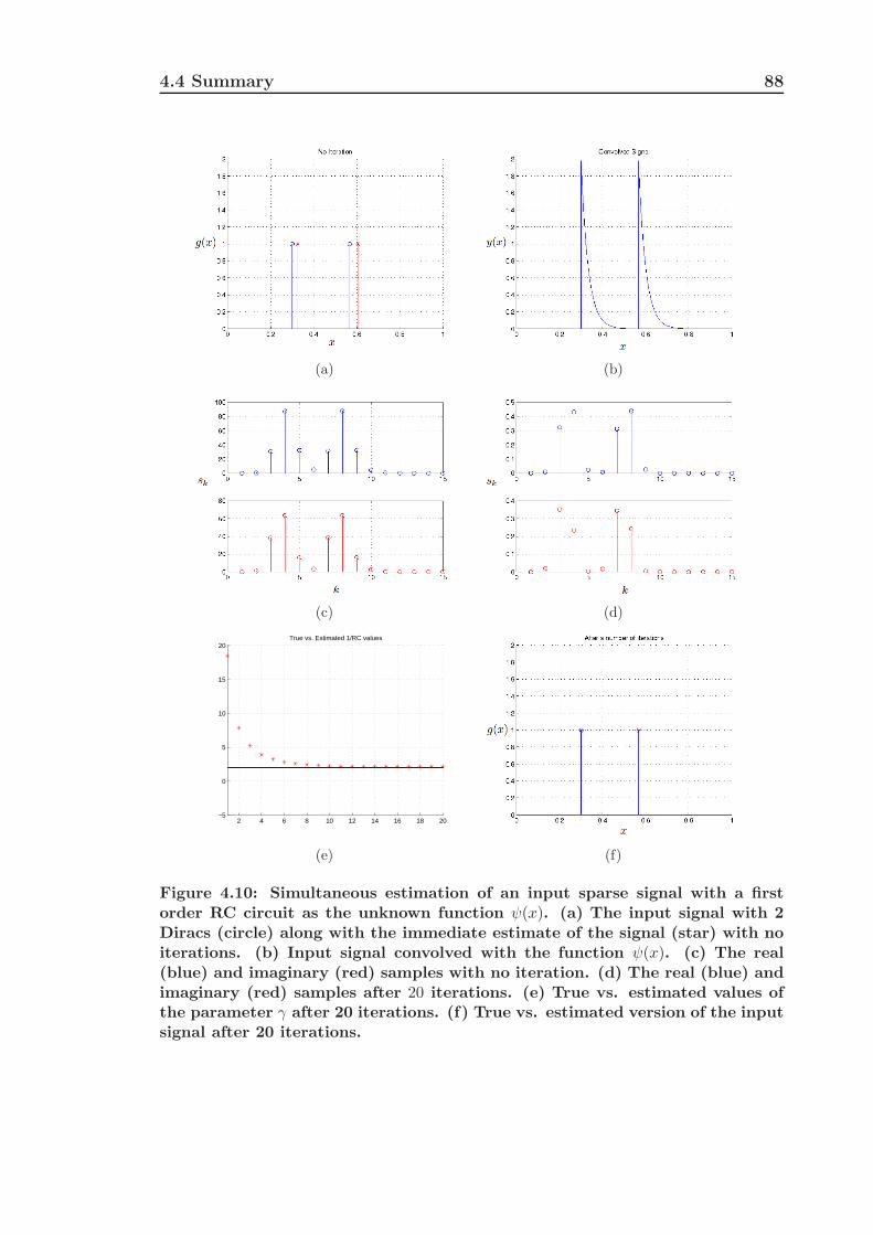
4.4 Summary 88
(a) (b)
(c) (d)
2 4 6 8 10 12 14 16 18 20−5
0
5
10
15
20True vs. Estimated 1/RC values
(e) (f)
Figure 4.10: Simultaneous estimation of an input sparse signal with a firstorder RC circuit as the unknown function ψ(x). (a) The input signal with 2Diracs (circle) along with the immediate estimate of the signal (star) with noiterations. (b) Input signal convolved with the function ψ(x). (c) The real(blue) and imaginary (red) samples with no iteration. (d) The real (blue) andimaginary (red) samples after 20 iterations. (e) True vs. estimated values ofthe parameter γ after 20 iterations. (f) True vs. estimated version of the inputsignal after 20 iterations.
89
Chapter 5
Multichannel Sampling of
Multidimensional FRI Signals
5.1 Introduction
In Chapter 3, we presented a possible extension of sampling one-dimensional FRI
signals to the case of multichannel acquisition systems. In the multichannel sampling
setup presented, we assumed that the input signal observed by the system and
also the channel parameters introduced within each channel (i.e. delay and gain
parameters), have a 1-D structure. In this chapter, we aim to extend the framework
presented in Chapter 3 to the multidimensional case, where both the input signal
and also the channel parameters have a two-dimensional structure. The motivation
of this extension comes from the fact that in applications such as acquisition of
images in a multi-camera system, the estimation of the 2-D input signal as well as
the 2-D channel parameters is required. Therefore, given the practical importance
of such setups, it is essential to analyse the case of multidimensional FRI signals.
The material of this chapter has been in part published in [4, 2, 3, 1].
The contribution of this chapter is two-fold; first, we present a novel approach
for sampling and perfectly reconstructing 2-D signals with parametric structure or
namely 2-D signals with FRI. The considered signals are bi-level polygons and set of
5.2 Multidimensional Sampling Framework 90
2-D Diracs and it will be shown that with the use of ACMP method (Algebraically
Coupled Matrix Pencils), projection-slice theorem, Radon projections and exponen-
tial splines as sampling kernels, such signals can be perfectly reconstructed from
their samples. Then, we consider the multichannel sampling of such 2-D signals and
demonstrate that a simultaneous channel synchronization and signal reconstruction
is possible. For the channel synchronization stage, we assume that the channel pa-
rameters are unknown geometric transformations such as translation, scaling, shear-
ing and rotation.
The organization of this chapter is as follows: In the next section, we will
introduce the multidimensional sampling framework for FRI signals which will in-
clude the definition of 2-D FRI signals, sampling setup used and the properties of
the sampling kernels involved. In Section 5.3 we will introduce our novel algorithms
for sampling and perfectly reconstructing set of 2-D Diracs by employing the ACMP
method and bi-level polygons by utilizing Radon transformation and its relationship
with the Fourier transform. In Section 5.4, we will extend the multichannel sampling
setup presented in Chapter 3, to the case of multichannel sampling of 2-D FRI sig-
nals and present our novel algorithm for signal and channel estimation under simple
2-D translations and also affine transformations. The summary of the chapter will
be given in Section 5.5.
5.2 Multidimensional Sampling Framework
5.2.1 2-D Signals with Finite Rate of Innovation
The definition of 2-D FRI signals is very similar to the 1-D case described in Chapter
2. Let us consider a 2-D signal with the following form:
g(x, y) =
N∑
r=0
∑
j∈Z
∑
k∈Z
γj,k,r φr(x− xj , y − yk). (5.1)
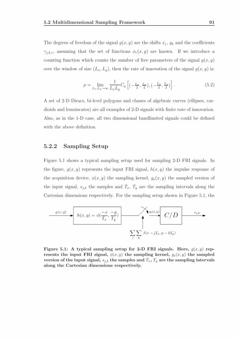
5.2 Multidimensional Sampling Framework 91
The degrees of freedom of the signal g(x, y) are the shifts xj , yk and the coefficients
γj,k,r, assuming that the set of functions φr(x, y) are known. If we introduce a
counting function which counts the number of free parameters of the signal g(x, y)
over the window of size (Lx, Ly), then the rate of innovation of the signal g(x, y) is:
ρ = limLx,Ly→∞
1
LxLy
Cg
[(−Lx
2, Lx
2), (−Ly
2, Ly
2)]. (5.2)
A set of 2-D Diracs, bi-level polygons and classes of algebraic curves (ellipses, car-
dioids and lemniscates) are all examples of 2-D signals with finite rate of innovation.
Also, as in the 1-D case, all two dimensional bandlimited signals could be defined
with the above definition.
5.2.2 Sampling Setup
Figure 5.1 shows a typical sampling setup used for sampling 2-D FRI signals. In
the figure, g(x, y) represents the input FRI signal, h(x, y) the impulse response of
the acquisition device, φ(x, y) the sampling kernel, gs(x, y) the sampled version of
the input signal, sj,k the samples and Tx, Ty are the sampling intervals along the
Cartesian dimensions respectively. For the sampling setup shown in Figure 5.1, the
Figure 5.1: A typical sampling setup for 2-D FRI signals. Here, g(x, y) rep-resents the input FRI signal, φ(x, y) the sampling kernel, gs(x, y) the sampledversion of the input signal, sj,k the samples and Tx, Ty are the sampling intervalsalong the Cartesian dimensions respectively.
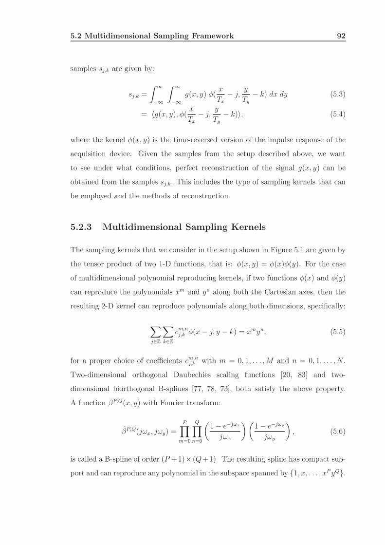
5.2 Multidimensional Sampling Framework 92
samples sj,k are given by:
sj,k =
∫ ∞
−∞
∫ ∞
−∞
g(x, y) φ(x
Tx− j,
y
Ty− k) dx dy (5.3)
= 〈g(x, y), φ( xTx
− j,y
Ty− k)〉, (5.4)
where the kernel φ(x, y) is the time-reversed version of the impulse response of the
acquisition device. Given the samples from the setup described above, we want
to see under what conditions, perfect reconstruction of the signal g(x, y) can be
obtained from the samples sj,k. This includes the type of sampling kernels that can
be employed and the methods of reconstruction.
5.2.3 Multidimensional Sampling Kernels
The sampling kernels that we consider in the setup shown in Figure 5.1 are given by
the tensor product of two 1-D functions, that is: φ(x, y) = φ(x)φ(y). For the case
of multidimensional polynomial reproducing kernels, if two functions φ(x) and φ(y)
can reproduce the polynomials xm and yn along both the Cartesian axes, then the
resulting 2-D kernel can reproduce polynomials along both dimensions, specifically:
∑
j∈Z
∑
k∈Z
cm,nj,k φ(x− j, y − k) = xmyn, (5.5)
for a proper choice of coefficients cm,nj,k with m = 0, 1, . . . ,M and n = 0, 1, . . . , N .
Two-dimensional orthogonal Daubechies scaling functions [20, 83] and two-
dimensional biorthogonal B-splines [77, 78, 73], both satisfy the above property.
A function βP,Q(x, y) with Fourier transform:
βP,Q(jωx, jωy) =
P∏
m=0
Q∏
n=0
(1− e−jωx
jωx
)(1− e−jωy
jωy
), (5.6)
is called a B-spline of order (P +1)× (Q+1). The resulting spline has compact sup-
port and can reproduce any polynomial in the subspace spanned by 1, x, . . . , xP yQ.
5.2 Multidimensional Sampling Framework 93
For the case of multidimensional exponential reproducing kernels, if two func-
tions φ(x) and φ(y) can reproduce real or complex exponentials along both the
Cartesian axes, then the resulting 2-D kernel can reproduce exponentials along both
dimensions, specifically:
∑
j∈Z
∑
k∈Z
cm,nj,k φ(x− j, y − k) = eαmxeβny, (5.7)
for a proper choice of coefficients cm,nj,k . The choice of the exponents is restricted to
αm = α0 +mλ1 and βn = β0 + nλ2 which is done to allow the use of specific recon-
struction techniques, and are described later on. E-splines [79] satisfy the property
defined in Equation (5.7) where a function β~α,~β
(x, y) with Fourier transform:
β~α,~β
(jωx, jωy) =
P∏
m=0
Q∏
n=0
(1− eαm−jωx
jωx − αm
)(1− eβn−jωy
jωy − βn
), (5.8)
is called an E-spline of order (P + 1) × (Q + 1) where ~α = (α0, α1, . . . , αP )
and ~β = (β0, β1, . . . , βQ) can be real or complex. The resulting spline has com-
pact support and can reproduce any exponential in the subspace spanned by
eα0xeβ0y, eα1xeβ0y, . . . , eαP xeβQy.
Interestingly, E-splines can be regarded as a generalized version of B-splines.
The reason is that, if we set the αm and βn parameters to zero, that is ~α = ~0 and
~β = ~0, then we obtain a 2-D B-spline of order (P +1)× (Q+1). Moreover, E-splines
can reproduce a combination of polynomials and exponentials. To illustrate this,
let us assume that the set of parameters αm and βn are ~α = (0, 0, 0, α3, α4, . . . , αP )
and ~β = (0, 0, 0, β3, β4, . . . , βQ) respectively. Then the resulting spline can reproduce
5.2 Multidimensional Sampling Framework 94
both polynomials and exponentials:
∑
j∈Z
∑
k∈Z
cm,nj,k φ(x− j, y − k) =
xm yn for m = 0, 1, 2, and n = 0, 1, 2
xm eβny for m = 0, 1, 2, and n = 3, 4, . . . , Q
eαmx yn for m = 3, 4, . . . , P, and n = 0, 1, 2
eαmx eβny for m = 3, 4, . . . , P, and n = 3, 4, . . . , Q.
(5.9)
The use of this feature will be explained later on.
5.2.4 Geometric and Exponential Moments
As in the 1-D case, the geometric or exponential moments can be estimated to
retrieve the degrees of freedom of g(x, y). In order to obtain the geometric or
exponential moments from the samples, let us consider τm,n to be:
τm,n =∑
j
∑
k
cm,nj,k sj,k, (5.10)
where cm,nj,k are the suitable coefficients used in Equation (5.5) or (5.7). By expanding
the samples sj,k we have (we have assumed that Tx = Ty = 1):
τm,n =∑
j
∑
k
cm,nj,k 〈g(x, y), φ(x− j, y − k)〉 (5.11)
= 〈g(x, y),∑
j
∑
k
cm,nj,k φ(x− j, y − k)〉. (5.12)
Assuming that a polynomial reproducing kernel is used as the sampling kernel
φ(x, y), then by substituting Equation (5.5) into the above equation, the 2-D geo-
5.3 Reconstruction Techniques 95
metric moments of the signal are obtained:
τm,n = 〈g(x, y),∑
j
∑
k
cm,nj,k φ(x− j, y − k)〉 (5.13)
= 〈g(x, y), xm yn〉 (5.14)
=
∫ ∞
−∞
∫ ∞
−∞
g(x, y) xm yn dx dy. (5.15)
Likewise, if an exponential reproducing kernel is used as the sampling kernel, then
by substituting Equation (5.7), the exponential moments of the signal are obtained:
τm,n = 〈g(x, y),∑
j
∑
k
cm,nj,k φ(x− j, y − k)〉 (5.16)
= 〈g(x, y), eαmxeβny〉 (5.17)
=
∫ ∞
−∞
∫ ∞
−∞
g(x, y) eαmxeβny dx dy. (5.18)
In the case of purely imaginary E-splines with αm = jmλ1 and βn = jnλ2, the
Fourier transform of the signal g(x, y) at (αm, βn) are obtained from the exponential
moments, that is:
τm,n = g(αm, βn). (5.19)
Here, g(jωx, jωy) represents the Fourier transform of the signal g(x, y).
5.3 Reconstruction Techniques
The problem of perfectly reconstructing 2-D FRI signals from their samples is more
involved and does not allow direct extension of the 1-D results. Recently, extensions
to the multidimensional case were considered by Maravic et al. [48] and Shukla et al.
[69]. Maravic et al. considered 2-D FRI signals, such as 2-D set of Diracs and bi-level
polygons and used the sinc and Gaussian sampling kernels to sample and perfectly
reconstruct such signals. Shukla et al. proposed algorithms, from the theory of
complex moments [21, 22, 54], for sampling the same 2-D signals but with the use
5.3 Reconstruction Techniques 96
of B-splines as the sampling kernel. As we previously mentioned, the sinc and the
Gaussian sampling kernels have infinite support and are not physically realizable.
Moreover, such kernels make the reconstruction algorithm unstable. In the following
sections we present our novel algorithms for sampling and perfectly reconstructing
2-D set of Diracs and bi-level polygons using E-spline sampling kernels.
5.3.1 A Sampling Theorem for 2-D Diracs
Let us assume that a set of 2-D Diracs is sampled with the sampling setup shown
in Figure 5.1. Assuming that there are K Diracs in the signal, such a signal can be
written as:
g(x, y) =
K∑
k=1
ak δ(x− xk, y − yk), (5.20)
where ak are the amplitudes and (xk, yk) are the coordinates of the Diracs respec-
tively. Since each Dirac has an amplitude and two coordinates, the signal has 3K
degrees of freedom. From the samples obtained, we first calculate the exponential
moments as follows:
τm,n =∑
j
∑
k
cm,nj,k sj,k (5.21)
=∑
j
∑
k
cm,nj,k
∫ ∞
−∞
∫ ∞
−∞
g(x, y) φ(x− j, y − k) dx dy (5.22)
=
∫ ∞
−∞
∫ ∞
−∞
g(x, y) eαmxeβny dx dy (5.23)
=K∑
k=1
ak
∫ ∞
−∞
∫ ∞
−∞
δ(x− xk, y − yk) eαmxeβny dx dy (5.24)
=
K∑
k=1
ak eαmxkeβnyk . (5.25)
We can see that the derived exponential moments τm,n has a 2-D power-sum series
form. Our aim is to estimate the parameters (ak, xk, yk) from τm,n. At first sight,
one might suggest an extension of the annihilating filter method for 1-D signals
described in Chapter 2 to this scenario. However, this extension fails because the
5.3 Reconstruction Techniques 97
relation τm,n ∗ hm,n = 0, where hm,n is the annihilating filter, is not unique for the
distinct locations (xk, yk) and thus there exists no unique solution to τm,n ∗hm,n = 0.
Another way to tackle this problem is by setting the indices m and n to zero
one at a time and applying the 1-D annihilating filter method on both sets to find
the values of xk and yk separately. There are two problems with this approach: first,
the estimated locations have to be paired and this is a combinatorial problem and
second, in the case of 2-D Diracs with a common coordinate, the annihilating filter
method is unable to find the multiple poles, because of having non-unique filter
coefficients.
This is indeed a spectral estimation problem and among the earliest tech-
niques that addressed this problem was the matrix enhancement and matrix pencil
(MEMP) algorithm by Hua [36]. For the case of common coordinates problem, Hua
solves the rank deficiency problem by introducing an enhanced matrix of the original
data matrix. In this way, a partitioned and stacked Hankel matrix of the original
data matrix is constructed in a way such that the full-rank property of the original
matrix is restored. For the pairing problem, an unattractive combinatorial approach
is suggested, trying all the possible combinations to find the correct pairing. The
combinatorial approach is computationally expensive and not efficient. The ACMP
(Algebraically Coupled Matrix Pencils) method by F. Vanpoucke et al. [82] however,
introduces a new technique to find the correct pairings by simultaneously solving
two algebraically related generalized eigenvalue equations. As the matrix enhance-
ment approach in [36] is not compatible with the algebraic pairing technique, an
alternative rank restoration technique is introduced. We will now briefly outline the
ACMP algorithm, but more detailed discussions can be found in [82].
Outline of the ACMP Method
Given αm = α0 +mλ1 and βn = β0 + nλ2, the obtained measurements τm,n, which
consists of a sum of K exponentials (complex or real) with unknown coordinate
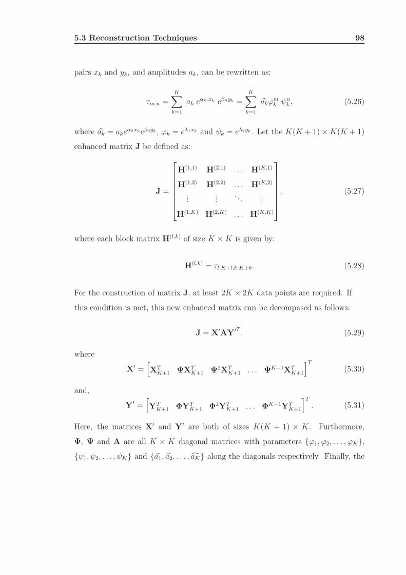
5.3 Reconstruction Techniques 98
pairs xk and yk, and amplitudes ak, can be rewritten as:
τm,n =K∑
k=1
ak eαmxk eβnyk =
K∑
k=1
akϕmk ψn
k , (5.26)
where ak = akeα0xkeβ0yk , ϕk = eλ1xk and ψk = eλ2yk . Let the K(K + 1)×K(K + 1)
enhanced matrix J be defined as:
J =
H(1,1) H(2,1) . . . H(K,1)
H(1,2) H(2,2) . . . H(K,2)
......
. . ....
H(1,K) H(2,K) . . . H(K,K)
, (5.27)
where each block matrix H(l,k) of size K ×K is given by:
H(l,k) = τl:K+l,k:K+k. (5.28)
For the construction of matrix J, at least 2K × 2K data points are required. If
this condition is met, this new enhanced matrix can be decomposed as follows:
J = X′AY′T , (5.29)
where
X′ =[XT
K+1 ΨXTK+1 Ψ2XT
K+1 . . . ΨK−1XTK+1
]T(5.30)
and,
Y′ =[YT
K+1 ΦYTK+1 Φ2YT
K+1 . . . ΦK−1YTK+1
]T. (5.31)
Here, the matrices X′ and Y′ are both of sizes K(K + 1) × K. Furthermore,
Φ, Ψ and A are all K × K diagonal matrices with parameters ϕ1, ϕ2, . . . , ϕK,ψ1, ψ2, . . . , ψK and a1, a2, . . . , aK along the diagonals respectively. Finally, the

5.3 Reconstruction Techniques 99
matrices XK+1 and YK+1 are given by:
XK+1 =
1 1 . . . 1
ϕ1 ϕ2 . . . ϕK
......
. . ....
ϕK1 ϕK
2 . . . ϕKK
YK+1 =
1 1 . . . 1
ψ1 ψ2 . . . ψK
......
. . ....
ψK1 ψK
2 . . . ψKK
. (5.32)
The matrices X′ and Y′ have a Vandermonde structure and when the matrix J
is at least of size K(K + 1) × K(K + 1), they are both full-rank . This matrix
enhancement technique restores the full-rank property of the original matrix for the
case of common coordinates problem [82]. Now, the four sub-matrices Jtl, Jtr, Jbl
and Jbr of matrix J are constructed, which correspond to the omission of the first
and last rows and columns on each block of the matrix J:
Jtl = J| = X′AY′T (5.33)
Jtr = |J = X′AY′T
(5.34)
Jbl = J| = X′AY′T (5.35)
Jbr = |J = X′AY′T. (5.36)
Here, over-line indicates the omission of the first row, under-line indicates the omis-
sion of the last row, left-line indicates the omission of the first column and right-line
indicates the omission of the last column of the matrices. Because of the Vander-
monde structure of the matrices X′ and Y′, it follows that:
Jtr = X′AΨY′T (5.37)
Jbl = X′ΦAY′T (5.38)
Jbr = X′ΦAΨY′T . (5.39)
From the matrices described above we can obtain two matrix pencils Jtr − µJtl and
Jbl − λJtl. The ACMP method then operates as follows: First the SVD of Jtl is
5.3 Reconstruction Techniques 100
computed:
Jtl = UΣVH, (5.40)
where H is Hermitian operator. By multiplying UH to the left hand side and
multiplying V to the right hand side of the two matrix pencils defined above we
obtain:
UH(Jtr − µJtl)V = UHX′AΨY′TV − µUHX′AY′TV (5.41)
= FΨG− µFG (5.42)
= Ctr − µCtl, (5.43)
and,
UH(Jbl − λJtl)V = UHX′AΦY′TV − λUHX′AY′TV (5.44)
= FΦG− λFG (5.45)
= Cbl − λCtl, (5.46)
where F = UHX′A, G = Y′TV, Ctr = UHJtrV = FΨG, Cbl = UHJblV = FΦG
and Ctl = UHJtlV = FG = Σ. By applying Eigen-value-decomposition (EVD) on
the new matrix pencils Ctr − µCtl and Cbl − λCtl, each of the poles ϕk and ψk are
obtained:
eig(C−1tl Ctr) = eig(G−1F−1FΨG) = eig(G−1ΨG) = Ψ (5.47)
eig(C−1tl Cbl) = eig(G−1F−1FΦG) = eig(G−1ΦG) = Φ. (5.48)
The identical transformation G on both equations guarantees that we have the
correct pairing for the estimated ϕk and ψk values. The steps below present a
pseudo code of the algorithm:
1. Construct the enhanced matrix J from the moments.
2. Construct the sub-matrices Jtl, Jtr and Jbl from the matrix J.
5.3 Reconstruction Techniques 101
3. Compute the singular value decomposition (SVD) of the sub-matrix Jtl, that
is Jtl = UΣVH.
4. Generate the matrices Ctl, Cbl and Ctr with the following equations: Ctl = Σ,
Ctr = UHJtrV, Cbl = UHJblV.
5. Apply the EVD to C−1tl Ctr and C−1
tl Cbl. This leads to the unknown poles
since: eig(C−1tl Ctr) = Ψ and eig(C−1
tl Cbl) = Φ.
As the exact values of the poles ϕk and ψk are found using the above method, the
matrices X′ and Y′ can now be constructed to obtain the parameters ak, using the
following equation:
A = (X′†)J(Y′T )†, (5.49)
where † stands for pseudo-inverse. From the estimated parameters ak and the poles
ϕk and ψk we can easily find the amplitudes ak and coordinates xk and yk as follows:
xk =ln(ϕk)
λ1, yk =
ln(ψk)
λ2, ak =
akeα0xkeβ0yk
. (5.50)
As mentioned above, for a set of K 2-D Diracs, at least 2K×2K data points
are required for the construction of the enhanced matrix. This means that the 2-D
E-spline order (P +1)× (Q+1) needs to be at least 2K× 2K in order to reproduce
the 2K exponential moments along both x and y axes. We can now summarize the
above discussion with the following proposition:
Proposition I - A set of K 2-D Diracs is uniquely determined from the
samples sj,k = 〈g(x, y), φ( xTx
− j, y
Ty− k)〉 provided that the sampling kernel φ(x, y),
can reproduce exponentials with an order 2K along both the Cartesian axes.
As an example, let us consider the input signal to be a set of 4 2-D Diracs
in a frame size of 256 × 256, shown in Figure 5.2(a). The signal is passed through
the E-spline sampling kernel of order 2K × 2K = 8× 8 shown in Figure 5.2(b) and
then sampled at the intervals Tx = Ty = 16, as shown in Figure 5.2(c). Given the
samples, the exponential moments are calculated and the ACMP method is applied
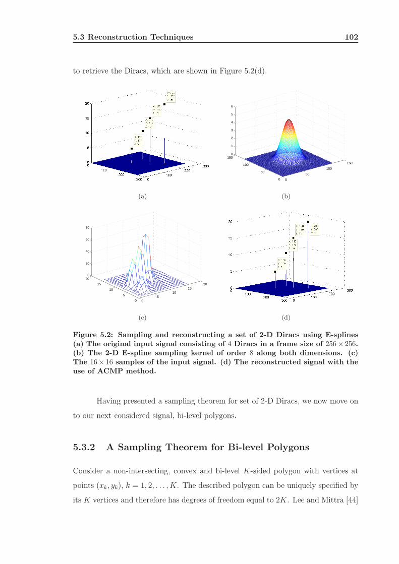
5.3 Reconstruction Techniques 102
to retrieve the Diracs, which are shown in Figure 5.2(d).
(a)
0
50
100
150
0
50
100
1500
1
2
3
4
5
6
(b)
05
1015
20
0
5
10
15
200
20
40
60
80
(c) (d)
Figure 5.2: Sampling and reconstructing a set of 2-D Diracs using E-splines(a) The original input signal consisting of 4 Diracs in a frame size of 256× 256.(b) The 2-D E-spline sampling kernel of order 8 along both dimensions. (c)The 16× 16 samples of the input signal. (d) The reconstructed signal with theuse of ACMP method.
Having presented a sampling theorem for set of 2-D Diracs, we now move on
to our next considered signal, bi-level polygons.
5.3.2 A Sampling Theorem for Bi-level Polygons
Consider a non-intersecting, convex and bi-level K-sided polygon with vertices at
points (xk, yk), k = 1, 2, . . . , K. The described polygon can be uniquely specified by
its K vertices and therefore has degrees of freedom equal to 2K. Lee and Mittra [44]
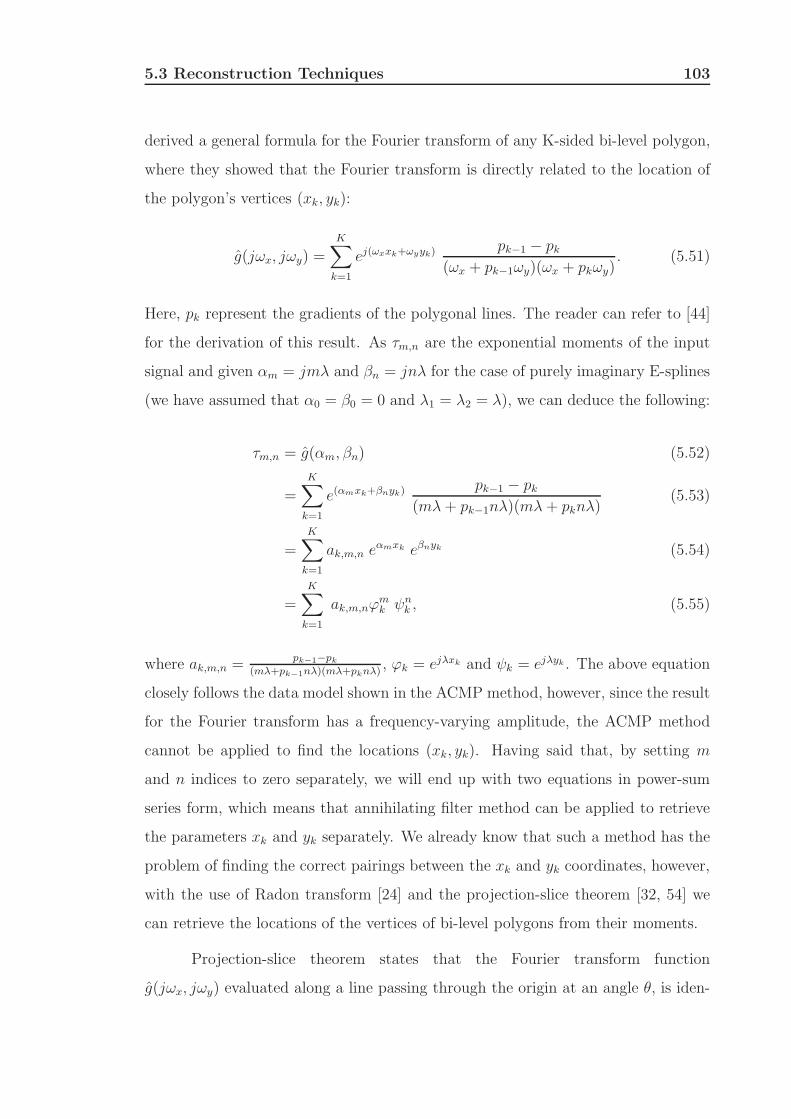
5.3 Reconstruction Techniques 103
derived a general formula for the Fourier transform of any K-sided bi-level polygon,
where they showed that the Fourier transform is directly related to the location of
the polygon’s vertices (xk, yk):
g(jωx, jωy) =K∑
k=1
ej(ωxxk+ωyyk)pk−1 − pk
(ωx + pk−1ωy)(ωx + pkωy). (5.51)
Here, pk represent the gradients of the polygonal lines. The reader can refer to [44]
for the derivation of this result. As τm,n are the exponential moments of the input
signal and given αm = jmλ and βn = jnλ for the case of purely imaginary E-splines
(we have assumed that α0 = β0 = 0 and λ1 = λ2 = λ), we can deduce the following:
τm,n = g(αm, βn) (5.52)
=
K∑
k=1
e(αmxk+βnyk)pk−1 − pk
(mλ+ pk−1nλ)(mλ+ pknλ)(5.53)
=
K∑
k=1
ak,m,n eαmxk eβnyk (5.54)
=K∑
k=1
ak,m,nϕmk ψn
k , (5.55)
where ak,m,n =pk−1−pk
(mλ+pk−1nλ)(mλ+pknλ), ϕk = ejλxk and ψk = ejλyk . The above equation
closely follows the data model shown in the ACMP method, however, since the result
for the Fourier transform has a frequency-varying amplitude, the ACMP method
cannot be applied to find the locations (xk, yk). Having said that, by setting m
and n indices to zero separately, we will end up with two equations in power-sum
series form, which means that annihilating filter method can be applied to retrieve
the parameters xk and yk separately. We already know that such a method has the
problem of finding the correct pairings between the xk and yk coordinates, however,
with the use of Radon transform [24] and the projection-slice theorem [32, 54] we
can retrieve the locations of the vertices of bi-level polygons from their moments.
Projection-slice theorem states that the Fourier transform function
g(jωx, jωy) evaluated along a line passing through the origin at an angle θ, is iden-
5.3 Reconstruction Techniques 104
tical to the one dimensional Fourier transform of the Radon projection Rg(x, θ). In
mathematical form:
g(jω cos(θ), jω sin(θ)) = Rg(jω, θ). (5.56)
In our setup, θ = tan−1( nm) with m and n being the indices of the moments and
ω =√(m2 + n2). With the help of this mapping, we can transform the Fourier
coefficients of bi-level polygons, obtained from purely imaginary E-spline sampling
kernel, to the Radon domain as follows:
Rg(jω, θ) = τωcos(θ), ωsin(θ)
=
K∑
k=1
pk−1 − pk(ωcos(θ) + pk−1ωsin(θ))(ωcos(θ) + pkωsin(θ))
eαωcos(θ)xk+βωsin(θ)yk
= ω−2K∑
k=1
ak,θ eαωcos(θ)xk+βωsin(θ) ,
where ak,θ = pk−1−pk(cos(θ)+pk−1sin(θ))(cos(θ)+pksin(θ))
. Let us introduce S(ω, θ) =
τωcos(θ), ωsin(θ) × ω2. The above equation can now be rewritten as:
S(ω, θ) =
K∑
k=1
ak,θ eαωcos(θ)xk+βωsin(θ)yk . (5.57)
At ω = 0, S(ω, θ) = 0 so the minimum required spline order can be decreased by 1 as
the first data sample is always zero. Since the angle θ is fixed for a given projection,
then the mapped equation at different projections has a power-sum series form:
Sθ(ω) =
K∑
k=1
akejωλzk =
K∑
k=1
akuωk , ω 6= 0, (5.58)
where ak = ak,θ, zk = xkcos(θ) + yksin(θ) and uk = ejλzk . By using the annihilating
filter method we can retrieve the parameters zk for each projection. For example,
by setting m = 0 and n = 0 we have the projections at θ = 0 and θ = 90 degrees
respectively, likewise if m = n then we have the projection at 45 degrees. Further
angles can be obtained by choosing different patterns such as m = 2n or n = 2m.
5.3 Reconstruction Techniques 105
Each projection, as explained above, will result in a power-sum series form and
annihilating filter method can be used to retrieve the parameters zk which correspond
to the sums of the vertices of the polygon in different directions. By back-projecting
the parameters zk according to their projection angle θ we are able to retrieve
some information about the polygon’s vertices. As any K-sided convex and bi-level
polygon is completely specified by the location of its K vertices, it is known [47]
that K +1 projections will entirely specify the vertices of the bi-level polygon, that
is, points that have K + 1 line intersections from the back-projections correspond
to the K vertices.
To reconstruct a set of K 1-D Diracs from its samples, we need at least
2K data points, which means a minimum spline order of 2K is required. For bi-
level polygons however, as the first data sample is always zero, a minimum number
of 2K − 1 exponential moments at each projection angle is required. Thus, the
minimum spline order required for a perfect reconstruction of a given K-sided bi-
level polygon is p.(2K − 1) − (p − 1) where p is the number needed in order to
produce at least K + 1 projections. For example for K = 3 or 4 the correct value
of is p = 2 and for K = 5, 6, 7, 8 the value is p = 3. The value of p can be found
by inspection but it can be shown that p is O(K), thus, the order of the spline is
O(K2) along both dimensions. We can now summarize the above discussion with
the following proposition:
Proposition II - A K-sided bi-level polygon is perfectly reconstructed from
the samples sj,k = 〈g(x, y), φ( xTx
− j, y
Ty− k)〉 provided that the sampling kernel
φ(x, y), can reproduce exponentials with an order p(2K − 1) − (p − 1) along both
dimensions, where p is the number required in order to produce at least K + 1
projections.
As an example, let us consider our input signal to be a bi-level triangle in
a frame size of 256 × 256, shown in Figure 5.3(a). The signal is passed through
the E-spline sampling kernel of order 9 × 9 and then sampled at intervals Tx =
Ty = 8, as shown in Figure 5.3(b). Given the samples, the exponential moments are
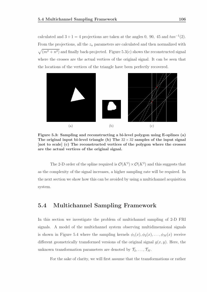
5.4 Multichannel Sampling Framework 106
calculated and 3+1 = 4 projections are taken at the angles 0, 90, 45 and tan−1(2).
From the projections, all the zn parameters are calculated and then normalized with√
(m2 + n2) and finally back-projected. Figure 5.3(c) shows the reconstructed signal
where the crosses are the actual vertices of the original signal. It can be seen that
the locations of the vertices of the triangle have been perfectly recovered.
(a) (b) (c)
Figure 5.3: Sampling and reconstructing a bi-level polygon using E-splines (a)The original input bi-level triangle (b) The 32× 32 samples of the input signal[not to scale] (c) The reconstructed vertices of the polygon where the crossesare the actual vertices of the original signal.
The 2-D order of the spline required is O(K2)×O(K2) and this suggests that
as the complexity of the signal increases, a higher sampling rate will be required. In
the next section we show how this can be avoided by using a multichannel acquisition
system.
5.4 Multichannel Sampling Framework
In this section we investigate the problem of multichannel sampling of 2-D FRI
signals. A model of the multichannel system observing multidimensional signals
is shown in Figure 5.4 where the sampling kernels φ1(x), φ2(x), . . . , φM(x) receive
different geometrically transformed versions of the original signal g(x, y). Here, the
unknown transformation parameters are denoted by T2, . . . , TM .
For the sake of clarity, we will first assume that the transformations or rather
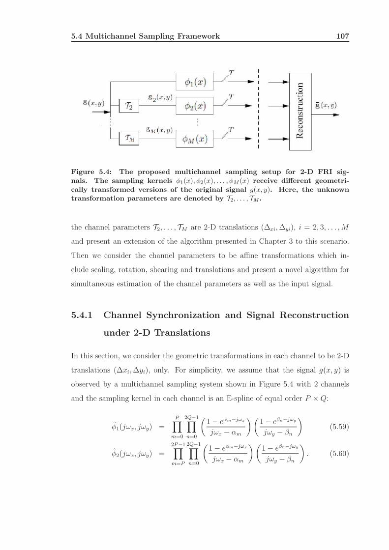
5.4 Multichannel Sampling Framework 107
Figure 5.4: The proposed multichannel sampling setup for 2-D FRI sig-nals. The sampling kernels φ1(x), φ2(x), . . . , φM (x) receive different geometri-cally transformed versions of the original signal g(x, y). Here, the unknowntransformation parameters are denoted by T2, . . . ,TM .
the channel parameters T2, . . . , TM are 2-D translations (∆xi,∆yi), i = 2, 3, . . . ,M
and present an extension of the algorithm presented in Chapter 3 to this scenario.
Then we consider the channel parameters to be affine transformations which in-
clude scaling, rotation, shearing and translations and present a novel algorithm for
simultaneous estimation of the channel parameters as well as the input signal.
5.4.1 Channel Synchronization and Signal Reconstruction
under 2-D Translations
In this section, we consider the geometric transformations in each channel to be 2-D
translations (∆xi,∆yi), only. For simplicity, we assume that the signal g(x, y) is
observed by a multichannel sampling system shown in Figure 5.4 with 2 channels
and the sampling kernel in each channel is an E-spline of equal order P ×Q:
φ1(jωx, jωy) =P∏
m=0
2Q−1∏
n=0
(1− eαm−jωx
jωx − αm
)(1− eβn−jωy
jωy − βn
)(5.59)
φ2(jωx, jωy) =
2P−1∏
m=P
2Q−1∏
n=0
(1− eαm−jωx
jωx − αm
)(1− eβn−jωy
jωy − βn
). (5.60)
5.4 Multichannel Sampling Framework 108
As shown above, we have set one parameter to be common between the exponents of
E-spline in one dimensions, specifically, both kernels can reproduce the exponentials
eαP xeβny for n = 0, 1, . . . , 2Q− 1. The samples of the i-th channel, with i = 1, 2, are
given by:
sij,k = 〈g(x−∆xi, y −∆yi), φ(x− j, y − k)〉, (5.61)
where (∆x1,∆y1) = (0, 0). Our goal is to have a reconstruction technique that can
perfectly retrieve the unknown translation parameters as well as the input signal.
Give the samples, we can obtain the exponential moments τ im,n for both channels:
τ 1m,n =
∫ ∞
−∞
∫ ∞
−∞
g(x, y) eαmxeβnydx dy, (5.62)
where m = 0, 1, . . . , P and n = 0, 1, . . . , 2Q− 1 and,
τ 2m,n =
∫ ∞
−∞
∫ ∞
−∞
g(x−∆x2, y −∆y2) eαmxeβnydx dy = τ 1m,ne
αm∆x2eβn∆y2, (5.63)
where m = P, P + 1, . . . , 2P − 1 and n = 0, 1, . . . , 2Q− 1. We can see that there is
a direct relationship between the exponential moments of the two signals. Now, by
taking logarithms on both sides of Equation (5.63), we obtain a system of simple
linear equations which we can solve for the translation parameters ∆x2 and ∆y2,
that is: ∆x2
∆y2
=
αP β0
αP β1
−1ln(
τ2P,0
τ1P,0
)
ln(τ2P,1
τ1P,1
)
. (5.64)
Given the exact translation parameters, we can now estimate the exponential mo-
ments τ 1m,n, with m = P, P + 1, ..., 2P − 1 from τ 2m,n as follows:
τ 1m,n = τ 2m,ne−αm∆x2e−βn∆y2, (5.65)
where m = P, P + 1, ..., 2P − 1 and n = 0, 1, . . . , 2Q− 1.
The result above, reveals that independently of g(x, y) it is possible to esti-
mate the channel parameters and synchronize the channels exactly from the obtained
5.4 Multichannel Sampling Framework 109
measurements. Therefore, once the channels are synchronized and the entire expo-
nential moments of the input signal are estimated, the corresponding reconstruction
algorithm, as described in Section 5.3.1 and 5.3.2, is applied to perfectly recover the
input signal. We now move on to the case where the transformation parameters are
affine transformations.
5.4.2 Channel Synchronization and Signal Reconstruction
under Affine Transformation
The above discussed method can be applied to any 2-D FRI signal as long as the
transformation parameters are restricted to 2-D translations. This is because intro-
ducing more complicated geometric transformations such as rotation, would result
in a non-linear relationship between the exponential moments of the different signals
and therefore our introduced method cannot be applied. However, we will show that
by employing a modified E-spline sampling kernel, the channel parameters and the
input signal can still be perfectly estimated.
Let us assume that we have a two-channel sampling system and the input
signal is a K-sided bi-level polygon (this method would also work for 2-D Diracs)
with affine transformation introduced in the second channel. Affine transformation
for 2-D signals is defined by a 6 degree parameter transformation and is defined as:
[x′ y′]T = A · [x y]T + [∆x ∆y]T , (5.66)
where [x y] represent the coordinates of the original signal, [x′ y′] represent the affine
transformed coordinates, [∆x ∆y] represents a 2-D translation and A is a 2 × 2
matrix. Matrix A is composed of a rotation parameter θ, 2-D scaling (Xscale, Yscale
and 2-D shearing (Xshear, Yshear), and is given as follows:
A =
A11 A12
A21 A22
=
cos(θ) − sin(θ)
sin(θ) cos(θ)
·
Xscale Xshear
Yshear Yscale
. (5.67)
5.4 Multichannel Sampling Framework 110
The unknown parameters of the affine transformation, can be estimated with the
use of geometric moments up to order 4 which can be obtained by a polynomial
reproducing kernel [29, 45, 86]. As we mentioned earlier, E-splines are a generalized
version of B-splines, thus, a combination of polynomials and exponentials from E-
splines can be reproduced. The Fourier transform of the corresponding modified
E-spline sampling kernel will then be as follows:
β~α,~β
(ωx, ωy) =
(1− e−jωx
jωx
)3(1− e−jωy
jωy
)3 P∏
m=0
Q∏
n=0
(1− eαm−jωx
jωx − αm
)(1− eβn−jωy
jωy − βn
).(5.68)
The produced spline is of order (P +1+ 4)× (Q+1+ 4), has compact support and
can reproduce polynomials up to order 4 along both dimensions and can reproduce
exponentials up to order (P +1)×(Q+1) (see Equation (5.9)). Therefore, the affine
parameters can be estimated from the modified sampling kernel. Given the channel
parameters, the next move is to recover the input signal.
As mentioned earlier, there is a non-linear relationship between the expo-
nential moments of the different signals. However, as affine transformation is an
invertible geometric transform, the following equation will also hold true:
[x y]T = A−1 ([x′ y′]T − [∆x ∆y]T ). (5.69)
Given the equation above, we propose our algorithm for signal estimation as follows:
First, we take two projections from the samples of the reference signal (i.e. first
channel) and then calculate its corresponding back-projections. This will lead to
K2 solutions. Then, at the same angles, we take two projections from the samples
of affine transformed signal and calculate its corresponding back-projections. This
will also lead to K2 solutions. We estimate the affine parameters from the geometric
moments of the two signals and then apply the inverted affine parameters, as was
shown in Equation (5.69), on each of the K2 solutions of the affine transformed
signal. We then map those points to the K2 solutions of the reference signal. The
mapped points that intersect with the K2 solutions of the reference signal, will be
5.4 Multichannel Sampling Framework 111
exactly K points and correspond to the vertices of the input bi-level polygon signal,
as long as A12 6= 0 and A21 6= 0.
To show that there are exactly K intersected points, let us consider g(x, y)
to have 2 Diracs at the positions (x1, y1) and (x2, y2) and let g′
(x, y) be an affine
transformed version of g(x, y). With 2 projections taken from the samples of each
signal at the angles 0 and 90 degrees, we will end up with K2 = 4 solutions for the
signal g(x, y) at the positions (x1, y1), (x1, y2), (x2, y1), (x2, y2) and K2 = 4 solutions
for the transformed signal g′
(x, y) at the positions (x′
1, y′
1), (x′
1, y′
2), (x′
2, y′
1), (x′
2, y′
2).
Given that the signal g′
(x, y) is an affine transformed version of the signal g(x, y),
we have:
x
′
1 = A11x1 + A12y1 +∆x
y′
1 = A21x1 + A22y1 +∆y
and
x
′
2 = A11x2 + A12y2 +∆x
y′
2 = A21x2 + A22y2 +∆y.
(5.70)
From the set of equations given above, we know that at least K = 2 points will
match to the correct points. Now, by considering the above equations, and applying
the affine transformation parameters on the rest of the solutions, that is at (x1, y2)
and (x2, y1), we have:
x
′
1 6= x′
2 6= A11x1 + A12y2 +∆x
y′
1 6= y′
2 6= A21x1 + A22y2 +∆y
and
x
′
2 6= x′
1 6= A11x2 + A12y1 +∆x
y′
2 6= y′
1 6= A21x2 + A22y1 +∆y,
(5.71)
where A12 6= 0 and A21 6= 0. Therefore, exactly K = 2 points will match, which are
the correct solutions. This will be true for any K as long as A12, A21 6= 0.
For the sake of clarity, the steps given below shows the procedures required
to sample bi-level polygons in our proposed multichannel framework with M = 2,
with affine transformation introduced on the second channel:
1. Choose the sampling kernel on both channels to be of equal order (2K − 1 +
4)× (2K − 1 + 4) where the number 4 corresponds to the spline order which
is required for estimating the affine transformation parameters and the order
5.4 Multichannel Sampling Framework 112
(2K − 1) × (2K − 1) corresponds to the minimum spline order required to
produce at least 2 projections for each signal (normally at 0 and 90 degree).
2. Estimate the affine transformation parameters between the two-channels from
their corresponding geometric moments.
3. Take two projections from the samples of both channels at the same angles and
compute their corresponding back-projections. This will lead to K2 solutions
for each of the signals.
4. Invert the estimated affine parameters and apply them (see Equation (5.69))
on each of the K2 solutions obtained from the second channel. Map those
points to the reference signal.
5. The mapped points that intersect with the K2 solutions of the reference signal
correspond to the K vertices of the input bi-level polygon signal.
As an example, let us consider the input signal to be a 4-sided bi-level polygon
shown in Figure 5.5(a), which is observed by a two-channel sampling system. The
second channel observes an affine transformed version of the input signal with the
following parameters: (∆x,∆y) = (90,−90)1, θ = 50, (Xscale, Yscale) = (1.05, 1.05)
and (Xshear, Yshear) = (0.5, 0.2), shown in Figure 5.5(b). Both signals are sampled
with an E-spline sampling kernel of order 2K − 1 + 4 = 11, shown in Figures
5.5(c)(d)(e). Two projections are taken at the angles 0 and 90 degrees for both
channels and this will lead to K2 = 16 solutions, as shown in Figure 5.5(f)(g). The
affine parameters, calculated from the geometric moments, are inverted and applied
to each of the K2 = 16 solutions of the affine transformed signal and then mapped
to the solutions of the reference signal, as shown in Figure 5.5(h). As can be seen,
only K = 4 points match with the K2 = 16 solutions, which correspond to the true
vertices of the input bi-level polygon.
1In pixels.
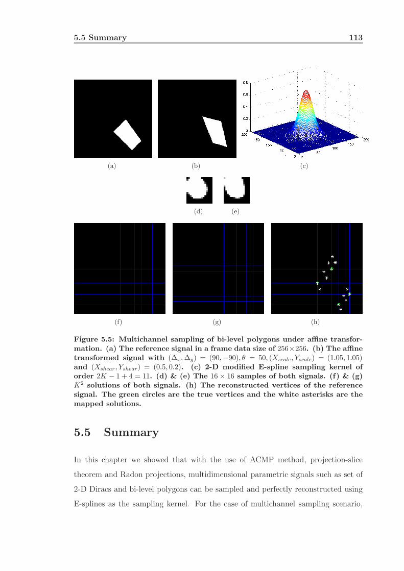
5.5 Summary 113
(a) (b) (c)
(d) (e)
(f) (g) (h)
Figure 5.5: Multichannel sampling of bi-level polygons under affine transfor-mation. (a) The reference signal in a frame data size of 256×256. (b) The affinetransformed signal with (∆x,∆y) = (90,−90), θ = 50, (Xscale, Yscale) = (1.05, 1.05)and (Xshear, Yshear) = (0.5, 0.2). (c) 2-D modified E-spline sampling kernel oforder 2K − 1 + 4 = 11. (d) & (e) The 16× 16 samples of both signals. (f) & (g)K2 solutions of both signals. (h) The reconstructed vertices of the referencesignal. The green circles are the true vertices and the white asterisks are themapped solutions.
5.5 Summary
In this chapter we showed that with the use of ACMP method, projection-slice
theorem and Radon projections, multidimensional parametric signals such as set of
2-D Diracs and bi-level polygons can be sampled and perfectly reconstructed using
E-splines as the sampling kernel. For the case of multichannel sampling scenario,

5.5 Summary 114
assuming that the geometric transformations are restricted to 2-D translations only,
we showed that the different channels can be synchronized regardless of the input
FRI signal. For the case of affine transformations however, we illustrated that,
with the use of modified E-splines and also taking affine transforms’ invertibility
into account, we can simultaneously estimate the channel parameters and the input
signal.
115
Chapter 6
Conclusion
In this thesis we presented a possible extension of the theory of sampling non-
bandlimited 1-D and 2-D signals with finite rate of innovation to the case of multi-
channel acquisition systems. What distinguishes our considered multichannel setup
to other setups is that, we assume each channel receives a disrupted version of the
observed input signal with some unknown parameters which could be delays and
gains in the 1-D case or affine transformations in the 2-D case. We posed both
the channel parameters estimation stage and the signal reconstruction stage as a
parametric estimation problem and demonstrated that a simultaneous exact syn-
chronization of the channels and reconstruction of the input 1-D and 2-D FRI signal
is possible. Furthermore, for the case of noisy measurements, we showed in this the-
sis that by considering the Cramer-Rao bounds as well as the numerical simulations,
the multichannel systems are more resilient to noise than the single-channel ones.
In the following section, we briefly summarize the contents of each chapter
of this thesis.
6.1 Thesis Summary
In Chapter 2, we presented a background on the 1-D sampling framework of FRI
signals. We described the different elements of the sampling setup used for sampling
6.1 Thesis Summary 116
FRI signals and showed how a set of 1-D Diracs can be sampled and perfectly
reconstructed using both polynomial and exponential reproducing kernels. Then
we considered the case of noisy scenario and presented some denoising techniques
such as matrix pencil method and Cadzow’s algorithm for the reconstruction of the
innovation parameters from the noisy samples.
In Chapter 3, we presented a possible extension of the theory of sampling
FRI signals to the case of multichannel acquisition systems. We showed that by
synchronizing the different channels of the proposed multichannel sampling setup,
one can estimate the unknown delays and gains introduced within the channels,
regardless of the input FRI signal. For the case of noisy measurements, we showed by
evaluating the CRB that, despite the fact that the unknown delays are required to be
estimated for synchronization, the number of samples required can be reduced by the
multichannel setup. Moreover, our numerical results with the multichannel sampling
setup revealed that the performance of the reconstruction algorithm improves over
the single-channel ones.
In Chapter 4, we proposed our novel algorithms for system identification
problem, based on the finite rate of innovation sampling theory. The novelty of this
chapter was divided into two section, where in the first section, we showed that by
having access to the input signal, system identification problem could be solved at
low sampling rates by employing the multichannel sampling setup and exponential
moments. Then, in the second section, we considered the problem of blind system
identification where we showed that a recursive method could be utilized to estimate
both the input FRI signal and also the unknown system when we only have access
to the output samples.
In Chapter 5, we first presented and discussed the sampling theory of multidi-
mensional FRI signals. We showed that with the use of ACMP method, projection-
slice theorem and Radon projections, multidimensional parametric signals such as
set of 2-D Diracs and bi-level polygons can be sampled and perfectly reconstructed
using exponential splines. For the case of multichannel sampling scenario, we first
6.2 Future Research 117
assumed that the geometric transformations are restricted to 2-D translations only
and showed that the different channels can be synchronized regardless of the input
FRI signal. Then we considered the case of affine transformations as the channel
parameters and illustrated that, with the use of modified E-splines we can simulta-
neously estimate the channel parameters as well as the input signal.
6.2 Future Research
There are many interesting while challenging open problems to look at in our re-
search work and some of them are given below:
Numerical Simulations versus Cramer-Rao Bounds
In Chapter 3, we theoretically showed that the described multichannel sampling sys-
tem is more resilient to noise than the single-channel ones. This was also confirmed
with our numerical simulations. However, none of the denoising methods employed
achieve the CRB and the gap between the CRB and the performance of the nu-
merical simulations is quite significant. Although sampling FRI signals under the
presence of noise has been extensively considered in [14], but we think that it will be
interesting to see if more robust and reliable algorithms for sampling complex FRI
signals under noisy conditions, such as adaptive hard-thresholding methods, can be
introduced.
Convergence of the Proposed Blind System Identification
Method
In Chapter 4, we mentioned that our empirical results show that by applying the
proposed method for blind system identification recursively, the estimations converge
to the actual input signal g(x) and the unknown function ψ(x). This was revealed
to us by taking a number of simulations with different parameters. However, a more

6.2 Future Research 118
subtle way to approach the convergence problem would be to provide a mathematical
evidence that the proposed method is convergent.
Proposed Sampling Theorem for Bi-level Polygons
In Chapter 5, we presented a novel algorithm for sampling and perfectly reconstruct-
ing bi-level polygons using E-splines, where we showed that by using the projection-
slice theorem, we can recover the vertices of bi-level polygons. Since for perfect
reconstruction K + 1 projections are needed for a K-sided bi-level polygon, the
order of E-spline used is O(N2) which is quite redundant when compared to the de-
grees of freedom of the signal O(2K). It would be interesting to find more efficient
ways of sampling and perfectly reconstructing bi-level polygons using E-splines.
The Potentials of E-splines
We have already mentioned that, E-splines are compact support splines that are
practically implementable and tend to be more stable than other kernels. Moreover,
from purely imaginary E-spline sampling kernels, the Fourier transform coefficients
of an input signal can be obtained. Therefore, they have a great potential to be
used as sampling kernels in various applications. For example, the model of neu-
ral signals are very similar to the model of E-splines convolved with Diracs and
therefore E-splines can have vast number of applications in neuroscience. We have
already considered E-splines for the problem of system identification in this thesis,
however, we think that more and more applications could benefit from these stable
and practically implementable sampling kernels.
119
Appendix A
Cramer-Rao Bound Derivation
Let us assume that we have an unbiased estimator Θ that is required to estimate a
vector of K unknown parameters from noisy samples sk. We denote the vector of
parameters by Θ as follows:
Θ = (Θ1,Θ2, . . . ,ΘK)T .
The measured noisy samples sk depend on the unknown parameters Θ and the
added noise ǫk, that is:
sk = f(Θ, k) + ǫk,
where we have assumed ǫk to be additive white Gaussian noise, independent of the
samples sk and the function f(Θ, k) is a function that depends on the vector Θ and
the sample index k. Since we have an unbiased estimator, we have:
E(Θ) = Θ.
The Cramer-Rao bound for any unbiased estimator Θ of the parameters Θ gives
the lowest achievable bound at a given noise level, and is given by the following
expression:
var(Θ) ≥ I−1(Θ),
A. Cramer-Rao Bound Derivation 120
where I(Θ) is the Fisher information matrix defined as:
I(Θ) = E(∇l(Θ) · ∇l(Θ)T ).
Here, l(Θ) is the log-likelihood function of Θ. The log-likelihood function of a set
of parameters Θ given the samples sk is defined by the probability of the samples
given the parameters Θ. Therefore, the log-likelihood function is given as follows:
l(Θ) = ln P (s0, s1, . . . , sN−1|Θ),
where P is the probability distribution of the samples conditioned on the parameters
Θ. Since ǫk is assumed to be white Gaussian with zero mean and variance σ2, the
probability distribution of ǫk is therefore given by [14, 26]:
pǫ(ǫk) =1√2πσ2
exp
(− ǫ2k2σ2
).
Given the probability distribution of the noise, we can deduce that:
ps(sk|Θ) = pǫ(g−1(sk))
∣∣∣∣∂g−1(sk)
∂sk
∣∣∣∣
=1√2πσ2
exp
(−(sk − f(Θ, k))2
2σ2
)
= pǫ(sk − f(Θ, k)),
A. Cramer-Rao Bound Derivation 121
where g(ǫk) = sk = f(Θ, k) + ǫk. Since the noise samples are independent, the
following can be deduced for the log-likelihood function:
l(Θ) = ln P (s0, s1, . . . , sN−1|Θ)
= ln
N−1∏
k=0
ps(sk|Θ)
=
N−1∑
k=0
ln ps(sk|Θ)
=N−1∑
k=0
ln pǫ(sk − f(Θ, k)).
To calculate the Fisher information matrix, we need to apply the divergence operator
on the log-likelihood function. Therefore we compute the partial derivatives of l(Θ)
with respect to the parameters Θ as follows:
∂l(Θ)
∂Θi
=∂l(Θ)
∂sk − f(Θ, k)
∂sk − f(Θ, k)
∂f(Θ, k)
∂f(Θ, k)
∂Θi
= −N−1∑
k=0
pǫpǫ(sk − f(Θ, k))
∂f(Θ, k)
∂Θi
=
N−1∑
k=0
sk − f(Θ, k)
σ2
∂f(Θ, k)
∂Θi
=1
σ2
N−1∑
k=0
ǫk∂f(Θ, k)
∂Θi
.
Thus,
∇l(Θ) =1
σ2
N−1∑
k=0
ǫk∇f(Θ, k).
A. Cramer-Rao Bound Derivation 122
Since the noise samples are independents and uncorrelated, the Fisher information
matrix can now be calculated as follows:
I(Θ) = E(∇l(Θ) · ∇l(Θ)T )
= E
(1
σ4
N−1∑
k=0
N−1∑
j=0
ǫkǫj∇f(Θ, k)∇f(Θ, k)T)
=1
σ4
N−1∑
k=0
N−1∑
j=0
δk,j∇f(Θ, k)∇f(Θ, k)T
=1
σ2
N−1∑
k=0
∇f(Θ, k)∇f(Θ, k)T .
Having obtained the Fisher information matrix, the Cramer-Rao bound, as men-
tioned previously, is given by the inverse of the Fisher information matrix:
CRB(Θ) = σ2
(N−1∑
k=0
∇f(Θ, k) · ∇f(Θ, k)T)−1
.
The CRB equation derived above only holds true for real-valued functions.
For the case of complex-valued E-spline sampling kernels, the samples are complex
valued and the noisy samples are assumed to be corrupted by complex AWGN,
defined as ǫk = uk + jvk where u and v are both real and independent random
variables with zero mean and σ2
2variance. The joint probability distribution of u
and v is given by:
pu,v(uk, vk) =1√2π σ2
2
exp
(− u2k2σ2
2
)· 1√
2π σ2
2
exp
(− v2k2σ2
2
)
=1
πσ2exp
(−u
2k + v2kσ2
)
=1
πσ2exp
(−|ǫn|2
σ2
)
= pǫ(ǫn),
where ǫn =√u2k + v2k. Given the probability distribution of the noise, the log-

A. Cramer-Rao Bound Derivation 123
likelihood function l(Θ) will be:
l(Θ) =
N−1∑
k=0
ln pǫ(sk − f(Θ, k)).
To calculate the Fisher information matrix, we need to apply the divergence operator
on the log-likelihood function like before. Applying a similar procedure will yield:
I(Θ) =2
σ2Re
(N−1∑
k=0
∇f(Θ, k) · ∇f ∗(Θ, k)
),
where ∗ stands for conjugate. The Cramer-Rao bound will therefore be as follows:
CRB(Θ) =σ2
2Re
(N−1∑
k=0
∇f(Θ, k) · ∇f ∗(Θ, k)
)−1
.

125
Bibliography
[1] H. Akhondi Asl and P.L. Dragotti. A sampling theorem for bilevel polygonsusing E-splines. In The 8th IMA International Conference on Mathematics inSignal Processing, Royal Agriculture College, Cirencester, UK, December 2008.
[2] H. Akhondi Asl and P.L. Dragotti. Multichannel sampling of translated, rotatedand scaled bilevel polygons using exponential splines. In The 8th internationalconference on Sampling Theory and Applications, Marseille, France, May 2009.
[3] H. Akhondi Asl and P.L. Dragotti. Single and multichannel sampling of bilevelpolygons using exponential splines. In IEEE International Conference onAcoustics, Speech, and Signal Processing, pages 3349–3352, Taipei, Taiwan,May 2009.
[4] H. Akhondi Asl and P.L. Dragotti. Multichannel sampling of multidimensionalparametric signals. To Appear in the Special Issue of Sampling Theory in Signaland Image Processing Journal, December 2011.
[5] H. Akhondi Asl, P.L. Dragotti, and L. Baboulaz. Multichannel sampling ofsignals with finite rate of innovation. IEEE Signal Processing Letter, 17(8):762–765, August 2010.
[6] L. Baboulaz. Feature Extraction for Image Super-resolution using Finite Rateof Innovation Principles. PhD thesis, Imperial College London, UK, 2008.
[7] L. Baboulaz and P.L. Dragotti. Distributed acquisition and image super-resolution based on continuous moments from samples. In IEEE InternationalConference on Image Processing (ICIP06), Atlanta (GA), October 2006.
[8] L. Baboulaz and P.L. Dragotti. Local feature extraction for image super-resolution. In IEEE International Conference on Image Processing (ICIP07),September 2007.
[9] L. Baboulaz and P.L. Dragotti. Exact feature extraction using finite rate of in-novation principles with an application to image super-resolution. IEEE Trans-actions on Image Processing, 18(2):281–298, February 2009.
[10] R. G. Baraniuk, E. Candes, R. Nowak, and M. Vetterli. Compressive sampling.IEEE Signal Processing Magazine, 25(2):12–13, March 2008.
Bibliography 126
[11] J. Berent, P.L. Dragotti, and T. Blu. Sampling piecewise sinusoidal signals withfinite rate of innovation methods. IEEE Transactions on Signal Processing,58(2):613–625, February 2010.
[12] W.C. Black and D.A. Hodges. Time interleaved converter arrays. IEEE Journalof Solid-State Circuits, 15(6):1022–1029, 1980.
[13] R.E. Blahut. Theory and practice of error control codes. Addison-Wesley, 1983.
[14] T. Blu, P.L. Dragotti, M. Vetterli, P. Marziliano, and L. Coulot. Sparse sam-pling of signal innovations: Theory, algorithms and performance bounds. IEEESignal Processing Magazine, 25(2):31–40, March 2008.
[15] T. Blu and M. Unser. Approximation errors for quasi-interpolators and (multi-)wavelet expansions. Applied and Computational Harmonic Analysis, 6 (2):219–251, March 1999.
[16] J.A. Cadzow. Signal enhancement- A composite property mapping algorithm.IEEE Transactions on Acoustics, Speech and Signal Processing, 36(1):49–62,January 1988.
[17] E. Candes, J. Romberg, and T. Tao. Robust uncertainty principle: Exact signalreconstruction from highly incomplete frequency information. IEEE Transac-tions on Information Theory, 52(2):489–509, February 2006.
[18] V. Chaisinthop and P.L Dragotti. Distributed video coding based on samplingof signals with finite rate of innovation. In Proc. of SPIE Conference on WaveletApplications in Signal and Image Processing, Wavelets XII, San Diego, USA,August 2007.
[19] Y. Chen, Y. Gu, and A.O. Hero-III. Sparse lms for system identification. InIEEE International Conference on Acoustics, Speech and Signal Processing,pages 3125–3128, 2009.
[20] I. Daubechies. Ten Lectures on Wavelets. Society for Industrial and AppliedMathematics, Philadelphia, USA, 1992.
[21] P.J. Davis. Triangle formulas in the complex plane. Mathematics of Computa-tion, 18(88):569–577, October 1964.
[22] P.J. Davis. Plane regions determined by complex moments. Journal of Approx-imation Theory, 19(2):148–153, 1977.
[23] B. De Moor. The singular value decomposition and long and short spacesof noisy matrices. IEEE Transactions on Signal Processing, 41(9):2826–2838,September 1993.
[24] S.R. Deans. The Radon transform and some of its applications. Wiley NewYork, 1983.
Bibliography 127
[25] D.L. Donoho. Compressed sensing. IEEE Transactions on Information Theory,52(4):1289–1306, April 2006.
[26] P.L. Dragotti and F. Homann. Sampling signals with finite rate of innovation inthe presence of noise. In IEEE International Conference on Acoustics, Speech,and Signal Processing, pages 2941–2944, April 2009.
[27] P.L. Dragotti, M. Vetterli, and T. Blu. Sampling moments and reconstructingsignals of finite rate of innovation: Shannon meets Strang-Fix. IEEE Transac-tions on Signal Processing, 55(5):1741–1757, May 2007.
[28] Y. Eldar. Compressed sensing of analog signals in shift-invariant spaces. IEEETransactions on Signal Processing, 57(8):2986–2997, August 2009.
[29] J. Flusser and T. Suk. A moment-based approach to registration of imageswith affine geometric distortion. IEEE Transactions on Geoscience and RemoteSensing, 32(2):382–387, March 1994.
[30] N. Gehrig and P.L. Dragotti. Distributed sampling and compression of sceneswith finite rate of innovation in camera sensor networks. In Data CompressionConference (DCC’06), March 2006.
[31] Y. Hao, P. Marziliano, M. Vetterli, and T. Blu. Compression of ECG as a signalwith finite rate of innovation. In The 27th Annual International Conference ofthe IEEE Engineering in Medicine and Biology Society, pages 7564–7567. IEEE,January 2005.
[32] G.T. Herman. Image Reconstruction from Projections: The Fundamentals ofComputerized Tomography. Academic Press, New York, 1980.
[33] A. Hormati, O. Roy, Lu. Y.M., and M. Vetterli. Distributed sampling of corre-lated signals linked by sparse filtering: Theory and applications. IEEE Trans-actions on Signal Processing, 58(3):1095–1109, March 2010.
[34] Y. Hua and T.K. Sarkar. Matrix pencil method and its performance. In IEEEInternational Conference on Acoustics, Speech, and Signal Processing, pages2476–2479, April 1988.
[35] Y. Hua and T.K. Sarkar. Matrix pencil method for estimating parameters ofexponentially damped/undamped sinusoids in noise. IEEE Transactions onAcoustics, Speech and Signal Processing, 38(5):814–824, May 1990.
[36] Y. Huy. Estimating two-dimensional frequencies by matrix enhancement andmatrix pencil. IEEE Transactions on Signal Processing, 40(9):2267–2280, Sep.1992.
[37] A.J. Jerri. The shannon sampling theorem- its various extensions and applica-tions: A tutorial review. Proceedings of the IEEE, 65(11):1565–1596, November1977.
Bibliography 128
[38] I. Jovanovic and B. Beferull-Lozano. Oversampled A/D conversion and error-rate dependence of nonbandlimited signals with finite rate of innovation. IEEETransactions on Signal Processing, 54(6):2140–2154, June 2006.
[39] V.A. Kotel’nikov. On the transmission capacity of the ether and cables in elec-trical communications. In Proceedings of the first All-Union Conference on thetechnological reconstruction of the communications sector and the developmentof low-current engineering. Moscow, 1933.
[40] V.A. Kotelnikov. On the transmission capacity of the ether and wire in elec-trocommunications. Modern Sampling Theory: Mathematics and Applications.Benedetto, J.J. and Ferreira, P. Birkhauser, Boston, MA, 2000.
[41] S.Y. Kung, K.S. Arun, and D.V. Bhaskar Rao. State-space and singular-valuedecomposition-based approximation methods for the harmonic retrieval prob-lem. Journal of Optical Society of America, 73(12):1799–1811, December 1983.
[42] J. Kusuma. Economical sampling of parametric signals. PhD thesis, Mas-sachusetts Institute of Technology, Cambridge, MA 02139, USA, 2006.
[43] J. Kusuma and V.K. Goyal. On the accuracy and resolution of powersum-basedsampling methods. IEEE Transactions on Signal Processing, 57(1):182–193,January 2009.
[44] S.W. Lee and R. Mittra. Fourier transform of a polygonal shape functionand its application in electromagnetics. IEEE Transactions on Antennas andPropagation, 31(1):99–103, January 1983.
[45] H. Li, B. S. Manjunath, and S. K. Mitra. A contour-based approach to multisen-sor image registration. IEEE Transactions on Image Processing, 4(2):320–334,March 1995.
[46] I. Maravic. Sampling methods for parametric non-bandlimited signals : exten-sions and applications. PhD thesis, Audio-Visual Communcation Laboratory,Swiss Federal Institute of Technology (EPFL), Lausanne, Switzerland, 2004.
[47] I. Maravic and M. Vetterli. A sampling theorem for the radon transform of finitecomplexity objects. In IEEE International Conference on Acoustics, Speech,and Signal Processing, volume 2, pages 1197–1200, Orlando, Florida (USA),May 2002.
[48] I. Maravic and M. Vetterli. Exact sampling results for some classes of para-metric nonbandlimited 2-D signals. IEEE Transactions on Signal Processing,52(1):175–189, January 2004.
[49] I. Maravic and M. Vetterli. Sampling and reconstruction of signals with fi-nite rate of innovation in the presence of noise. IEEE Transactions on SignalProcessing, 53(8):2788–2805, August 2005.
Bibliography 129
[50] I. Maravic, M. Vetterli, and K. Ramchandran. Channel estimation and syn-chronization with sub-Nyquist sampling and application to ultra-wideband sys-tems. In Proceedings of the International Symposium on Circuits and Systems(ISCAS’04), May 2004.
[51] F.A. Marvasti. Nonuniform sampling: theory and practice. Springer, NY, US,2001.
[52] P. Marziliano. Sampling innovations. PhD thesis, Audio-Visual CommuncationLaboratory, Swiss Federal Institute of Technology (EPFL), Lausanne, Switzer-land, 2001.
[53] M. McCormick and M. Lu, Y. M. Vetterli. Learning sparse systems at sub-nyquist rates: A frequency-domain approach. In IEEE International Conferenceon Acoustics, Speech, and Signal Processing, Dallas, Texas, USA, March 2010.
[54] P. Milanfar, G.C. Verghese, W.C. Karl, and A.S. Willsky. Reconstructing poly-gons from moments with connections to array processing. IEEE Transactionson Signal Processing, 43(2):432–443, February 1995.
[55] T.K. Moon and W.C. Stirling. Mathematical methods and algorithms for signalprocessing, volume 204. Prentice Hall, New York, 2000.
[56] H. Nyquist. Certain topics in telegraph transmission theory. Transactions ofthe American Institute of Electrical Engineers, 47(2):617–644, 1928.
[57] H. Olkkonen and J.T. Olkkonen. Measurement and reconstruction of impulsetrain by parallel exponential filter. IEEE Signal Processing Letter, 15:241–244,February 2008.
[58] A. Papoulis. Generalized sampling expansions. IEEE Transactions on CircuitsSyst., 24:652–654, November 1977.
[59] V.F. Pisarenko. The retrieval of harmonics from a covariance function. Geo-physical Journal of the Royal Astronomical Society, 33(3):347–366, September1973.
[60] B.D. Rao and K.S. Arun. Model based processing of signals: a state spaceapproach. IEEE Transactions on Signal Processing, 80(2):283–309, February1992.
[61] R. Roy and T. Kailath. ESPRIT-estimation of signal parameters via rotationalinvariance techniques. IEEE Transactions on Acoustics, Speech and Signal Pro-cessing, 37(7):984 –995, July 1989.
[62] T.K. Sarkar and O. Pereira. Using the matrix pencil method to estimate theparameters of a sum of complex exponentials. Antennas and Propagation Mag-azine, IEEE, 37(1):48–55, February 1995.
Bibliography 130
[63] A.H. Sayed. Adaptive filters. Wiley-IEEE Press, 2008.
[64] R. Schmidt. Multiple emitter location and signal parameter estimation. IEEETransactions on Antennas and Propagation, 34(3):276 – 280, March 1986.
[65] I. J. Schoenberg. Contribution to the problem of approximation of equidistantdata by analytic functions. Quarterly of Applied Mathematics, 4(2):45–99 and112–141, 1946.
[66] C.S. Seelamantula and M. Unser. A generalized sampling method for finite-rate-of-innovation-signal reconstruction. IEEE Signal Processing Letter, 15:813–816,November 2008.
[67] C.E. Shannon. Communication in the presence of noise. Proceedings of theIRE, 37(1):10–21, January 1949.
[68] P. Shukla. Sampling schemes for multidimensional nonbandlimited signals. PhDthesis, Imperial College London, UK, 2007.
[69] P. Shukla and P.L. Dragotti. Sampling schemes for multidimensional sig-nals with finite rate of innovation. IEEE Transactions on Signal Processing,55(7):3670–3686, July 2007.
[70] P. Stoica and R. Moses. Spectral Analysis of Signals. Prentice Hall, April 2005.
[71] G. Strang and G. Fix. A Fourier analysis of the finite element variationalmethod. In Constructive Aspect of Functional Analysis, pages 796–830, Rome(Italy), 1971.
[72] D.W. Tufts and R. Kumaresan. Estimation of frequencies of multiple sinusoids:Making linear prediction perform like maximum likelihood. Proceedings of theIEEE, 70(9):975–989, September 1982.
[73] M. Unser. Splines: A perfect fit for signal and image processing. IEEE SignalProcessing Magazine, 16(6):22–38, August 1999.
[74] M. Unser. Sampling-50 years after shannon. Proceedings of the IEEE,88(4):569–587, April 2000.
[75] M. Unser. Cardinal exponential splines: part II-think analog, act digital. IEEETransactions on Signal Processing, 53(4):1439–1449, March 2005.
[76] M. Unser and A. Aldroubi. A general sampling theory for nonideal acquisitiondevices. IEEE Transactions on Signal Processing, 42(11):2915–2925, November1994.
[77] M. Unser, A. Aldroubi, and M. Eden. B-spline signal processing. I- theory.IEEE Transactions on Signal Processing, 41(2):821 –833, February 1993.
Bibliography 131
[78] M. Unser, A. Aldroubi, and M. Eden. B-spline signal processing. II- efficiencydesign and applications. IEEE Transactions on Signal Processing, 41(2):834–848, February 1993.
[79] M. Unser and T. Blu. Cardinal exponential splines: Part I-theory and filteringalgorithms. IEEE Transactions on Signal Processing, 53(4):1425–1438, April2005.
[80] M. Unser and J. Zerubia. Generalized sampling: Stability and performanceanalysis. IEEE Transactions on Signal Processing, 45(12):2941–2950, December1997.
[81] M. Unser and J. Zerubia. A generalized sampling theory without bandlimitingconstraints. IEEE Transactions on Circuits Syst. II, 45(8):959–969, August1998.
[82] F. Vanpoucke, M. Moonen, and Y. Berthoumieu. Efficient subspace algorithmfor 2-D harmonic retrieval. In IEEE International Conference on Acoustics,Speech, and Signal Processing, volume 4, pages 461–464, Toulouse (France),April 1994.
[83] K. Vetterli and J. Kovacevic. Wavelets and Subband Coding. Prentice-Hall,1995.
[84] M. Vetterli, P. Marziliano, and T. Blu. Sampling signals with finite rate ofinnovation. IEEE Transactions on Signal Processing, 50(6):1417–1428, June2002.
[85] J.M. Whittaker. The Fourier theory of the cardinal function. Proceedings ofthe Edinburgh Mathematical Society (Series 2), 1(03):169–176, 1928.
[86] Z. Yang and F. Cohen. Cross-weighted moments and affine invariants for im-age registration and matching. IEEE Transactions on Pattern Analysis andMachine Iintelligence, 21(8):804–814, August 1999.