J. Acoustic Emission, 20 (2002) 39 © 2002 Acoustic Emission Group

A WAVELET TRANSFORM APPLIED TO ACOUSTIC EMISSIONSIGNALS: PART 1: SOURCE IDENTIFICATION #

M. A. HAMSTAD+, A. O�GALLAGHER and J. GARY

National Institute of Standards and Technology, Materials Reliability Division (853), Boulder,CO 80305-3328;

+Also Department of Engineering, University of Denver, Denver, CO 80208.

Abstract

A database of wideband acoustic emission (AE) modeled signals was used in Part 1 to ex-amine the application of a wavelet transform (WT) to identify AE sources. The AE signals in thedatabase were created by use of a validated three-dimensional finite element code. These signalsrepresented the out-of-plane displacements from buried dipole sources in aluminum plates 4.7mm thick and of small and large lateral dimensions. The surface displacement signals at threefar-field distances were filtered with a 40 kHz high-pass filter prior to applying the WT. TheWTs were calculated with AGU-Vallen Wavelet, a freeware software program. The effects ofpropagation distance, AE source type, and the depth of the AE source below the plate surfacewere examined. Specifically, a ratio of the WT magnitude (WT coefficient) from the fundamen-tal anti-symmetric mode to that from the fundamental symmetric mode was studied for correla-tion with the AE source type. The WT magnitudes were those corresponding to a particulargroup velocity and signal frequency for each mode. For sources in the large plate located at thesame depth, the ratios were able to distinguish different source types and exhibited only smallchanges with increasing propagation distance. But, when the variable of depth of the source wasintroduced, the ratios did not uniquely classify the AE source type. In the case of the small cou-pon plate specimen, reflections from the specimen edges distorted and complicated the WTs.Since the current coupon database excludes (except for one case) the parameter of changes in thedistance of the source from the coupon sides, a full examination of these complications was notpossible.

1. Introduction

Since early in the history of AE, a goal of AE practitioners has been to use AE signals as themeans to identify the type of source that generated the signals (Mehan and Mullin, 1971). Papershave been published indicating the successful identification of AE sources, and commercial AEcompanies offer software for the purpose of identifying AE sources. These efforts are often con-troversial because they lack an analytical justification (based on the theory of AE) of the signalfeatures used to sort the experimental signals into different types of sources. Alternatively, someAE source-identification experiments have been carried out with specimen geometries and sen-sor locations such that signals are obtained from the direct longitudinal bulk waves in severaldirections of radiation (Buttle and Scruby, 1990a). The analysis that is used to sort these signalsinto different source types (or combinations of source types) is based on analytical calculations(forward modeling) that determine the relative amplitudes of the first bulk longitudinal signals indifferent radiation directions. By comparing relative experimental bulk wave amplitudes in dif-ferent directions with the calculated results for a series of possible sources, the experimental# Contribution of the U.S. National Institute of Standards and Technology; not subject to copyright in the US.

40

sources were identified in a more satisfying fashion. However, in many AE applications Lambwaves are present due to plate-like test specimens and observation of the AE signals in the far-field. In this case, this more satisfying approach is not directly applicable. Some AE researchers(Weaver and Pao, 1982a, b; Guo et al., 1998) have presented analytical results (forward model-ing) for Lamb waves in infinite plates, but to date they have not published an extensive databasethat could lead to source identification of experimental signals by appropriate comparisons.

The AE source-identification research presented here uses an extensive database of modeledLamb-wave AE signals. These signals were obtained by use of a validated finite-element mod-eling code (Hamstad et al., 1999). Since the exact source type and all its characteristics areknown for each signal, the features of the AE signals can be unequivocally associated with par-ticular source types. In the case of experimental signals, this is not the case. In this paper we ex-amine the possibilities of extracting meaningful source identification features by the use of awavelet transform (WT). To retain the possibility of a direct method of source identification(rather that an artificial-intelligence method), this paper examines the extraction of limited datasets from the WT results. In addition, if the direct method is not completely successful, these re-sults could provide insight into the most relevant WT results to input into an artificial-intelligence approach.

2. Description of AE Database

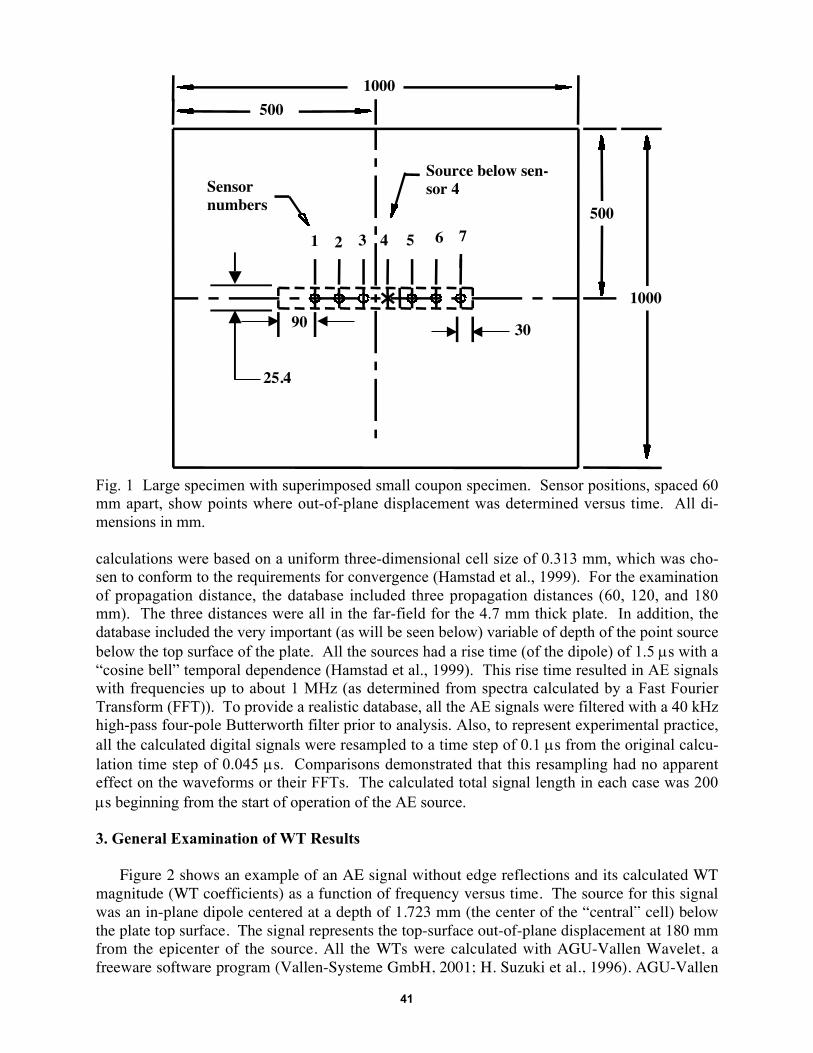
The AE signals that comprised the analyzed database were all calculated by the NIST- Boul-der finite-element modeling (FEM) code. This code has been validated (Hamstad et al., 1999;Prosser et al., 1999) for buried dipole-type point sources operating in plate specimens with infi-nite lateral dimensions and for surface and edge monopole sources on plates with small and largelateral dimensions. The specimen domains in the database were aluminum plates 4.7 mm thick.These plates had lateral dimensions of either 1000 mm by 1000 mm (representing the infinite-plate case) or 480 mm by 25.4 mm (representing a small coupon specimen). Figure 1 shows adrawing of the small specimen superimposed on the large specimen. The lateral position of theAE source and the positions where the plate top surface out-of-plane displacement was deter-mined as a function of time are shown. These displacement signals provide the AE signals thatwould be obtained in a single direction of radiation (toward sensors 1, 2 and 3) or the oppositedirection (toward sensors 5, 6, and 7). All the sensor positions were 60 mm apart.

The calculated signals provided a unique and ideal database that was far superior to experi-mental AE signals for the study of AE source identification. The reasons for this superiority aredue to exact knowledge of key information not always available in experimental data: point-source location in three dimensions; source rise time; magnitude and orientation of source di-poles; absolute out-of-plane displacement of a perfect wideband point sensor at an exact loca-tion; known filtering of the AE signal; signals both with specimen edge reflections and withoutsuch reflections; and signals that are largely free of noise.

For this study of AE source identification, the analyzed database included three types ofburied point-sources: (1) in-plane dipole, aligned with the propagation direction to the sensors,(2) out-of-plane dipole, and (3) crack initiation (three dipoles) with the largest dipole alignedwith the propagation direction to the sensors. The dipole forces (body forces) were all 1 N ex-cept for the two smaller dipoles in the microcrack case, which were 0.52 N (based on the elasticconstants of aluminum). Each dipole was made up of a �central� cell having no body force,along with single cells on each side of the �central� cell having body forces. All the

41

Fig. 1 Large specimen with superimposed small coupon specimen. Sensor positions, spaced 60mm apart, show points where out-of-plane displacement was determined versus time. All di-mensions in mm.

calculations were based on a uniform three-dimensional cell size of 0.313 mm, which was cho-sen to conform to the requirements for convergence (Hamstad et al., 1999). For the examinationof propagation distance, the database included three propagation distances (60, 120, and 180mm). The three distances were all in the far-field for the 4.7 mm thick plate. In addition, thedatabase included the very important (as will be seen below) variable of depth of the point sourcebelow the top surface of the plate. All the sources had a rise time (of the dipole) of 1.5 µs with a�cosine bell� temporal dependence (Hamstad et al., 1999). This rise time resulted in AE signalswith frequencies up to about 1 MHz (as determined from spectra calculated by a Fast FourierTransform (FFT)). To provide a realistic database, all the AE signals were filtered with a 40 kHzhigh-pass four-pole Butterworth filter prior to analysis. Also, to represent experimental practice,all the calculated digital signals were resampled to a time step of 0.1 µs from the original calcu-lation time step of 0.045 µs. Comparisons demonstrated that this resampling had no apparenteffect on the waveforms or their FFTs. The calculated total signal length in each case was 200µs beginning from the start of operation of the AE source.

3. General Examination of WT Results

Figure 2 shows an example of an AE signal without edge reflections and its calculated WTmagnitude (WT coefficients) as a function of frequency versus time. The source for this signalwas an in-plane dipole centered at a depth of 1.723 mm (the center of the �central� cell) belowthe plate top surface. The signal represents the top-surface out-of-plane displacement at 180 mmfrom the epicenter of the source. All the WTs were calculated with AGU-Vallen Wavelet, afreeware software program (Vallen-Systeme GmbH, 2001; H. Suzuki et al., 1996). AGU-Vallen

Sensornumbers

Source below sen-sor 4

25.4

1000

500

1000

500

90 30

1 2 3 4 5 6 7

42

Fig. 2 Typical calculated AE signal from an in-plane dipole source with corresponding WT.Superimposed fundamental symmetric, So, and anti-symmetric, Ao, modes after convertinggroup velocity to time based on 180 mm propagation distance. Red color corresponds to highestmagnitude of the WT. Source depth is 1.723 mm in large specimen. (WT scale: 1 MHz: 150 µs)

Wavelet has been developed in collaboration between Vallen-Systeme GmbH and AoyamaGakuin University (AGU), Tokyo, Japan. The AGU group has pioneered in the research ofwavelet analysis in the field of acoustic emission (Suzuki et al., 1996; Takemoto et al., 2000;Yamada et al., 2000). This program has a Gabor function as the �mother� wavelet with a centralfrequency of 7 MHz. The software program also includes a program to calculate the relevantgroup-velocity curves for the lowest ten modes of the infinite number of Lamb modes that gov-ern the far-field wave propagation in a plate. Figure 2 shows the two lowest modes (fundamentalsymmetric, So, and anti-symmetric, Ao) superimposed on the WT. This superposition is facili-tated by an option that converts the group velocity scale to a time scale using the known exactpropagation distance. The group-velocity curves were calculated by use of the same bulk ve-locities that were used in the finite-element computations (6,320 m/s bulk longitudinal velocityand 3,100 m/s bulk shear velocity). The FEM calculation also uses the material density of 2700kg/m3. The color scale in Fig. 2 is a linear scale with red representing the highest-magnitude re-gion of the WT and pink the smallest or zero-magnitude region. The display includes an optionto change the color scale (called the color factor) so as to include a greater or lesser portion ofthe maximum magnitudes in the �red� region. The WT in Fig. 2 has a color-factor (CF) value of0.8. A color factor of less than 1 (the default value) means that a wider range of the WT peakmagnitudes are displayed in red. The converse applies for color factors greater than 1.

A0

S0

43

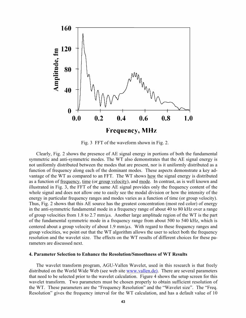
Fig. 3 FFT of the waveform shown in Fig. 2.

Clearly, Fig. 2 shows the presence of AE signal energy in portions of both the fundamentalsymmetric and anti-symmetric modes. The WT also demonstrates that the AE signal energy isnot uniformly distributed between the modes that are present, nor is it uniformly distributed as afunction of frequency along each of the dominant modes. These aspects demonstrate a key ad-vantage of the WT as compared to an FFT. The WT shows how the signal energy is distributedas a function of frequency, time (or group velocity), and mode. In contrast, as is well known andillustrated in Fig. 3, the FFT of the same AE signal provides only the frequency content of thewhole signal and does not allow one to easily see the modal division or how the intensity of theenergy in particular frequency ranges and modes varies as a function of time (or group velocity).Thus, Fig. 2 shows that this AE source has the greatest concentration (most red color) of energyin the anti-symmetric fundamental mode in a frequency range of about 40 to 80 kHz over a rangeof group velocities from 1.8 to 2.7 mm/µs. Another large amplitude region of the WT is the partof the fundamental symmetric mode in a frequency range from about 500 to 540 kHz, which iscentered about a group velocity of about 1.9 mm/µs. With regard to these frequency ranges andgroup velocities, we point out that the WT algorithm allows the user to select both the frequencyresolution and the wavelet size. The effects on the WT results of different choices for these pa-rameters are discussed next.

4. Parameter Selection to Enhance the Resolution/Smoothness of WT Results

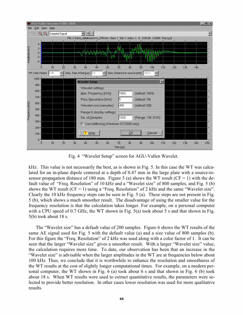
The wavelet transform program, AGU-Vallen Wavelet, used in this research is that freelydistributed on the World Wide Web (see web site www.vallen.de). There are several parametersthat need to be selected prior to the wavelet calculation. Figure 4 shows the setup screen for thiswavelet transform. Two parameters must be chosen properly to obtain sufficient resolution ofthe WT. These parameters are the �Frequency Resolution� and the �Wavelet size�. The �Freq.Resolution� gives the frequency interval for the WT calculation, and has a default value of 10

44

Fig. 4 �Wavelet Setup� screen for AGU-Vallen Wavelet.

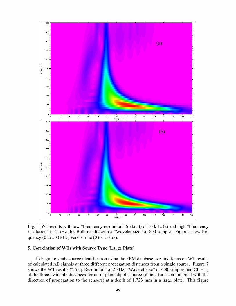
kHz. This value is not necessarily the best, as is shown in Fig. 5. In this case the WT was calcu-lated for an in-plane dipole centered at a depth of 0.47 mm in the large plate with a source-to-sensor propagation distance of 180 mm. Figure 5 (a) shows the WT result (CF = 1) with the de-fault value of �Freq. Resolution� of 10 kHz and a �Wavelet size� of 800 samples, and Fig. 5 (b)shows the WT result (CF = 1) using a �Freq. Resolution� of 2 kHz and the same �Wavelet size�.Clearly the 10 kHz frequency steps can be seen in Fig. 5 (a). These steps are not present in Fig.5 (b), which shows a much smoother result. The disadvantage of using the smaller value for thefrequency resolution is that the calculation takes longer. For example, on a personal computerwith a CPU speed of 0.7 GHz, the WT shown in Fig. 5(a) took about 5 s and that shown in Fig.5(b) took about 18 s.

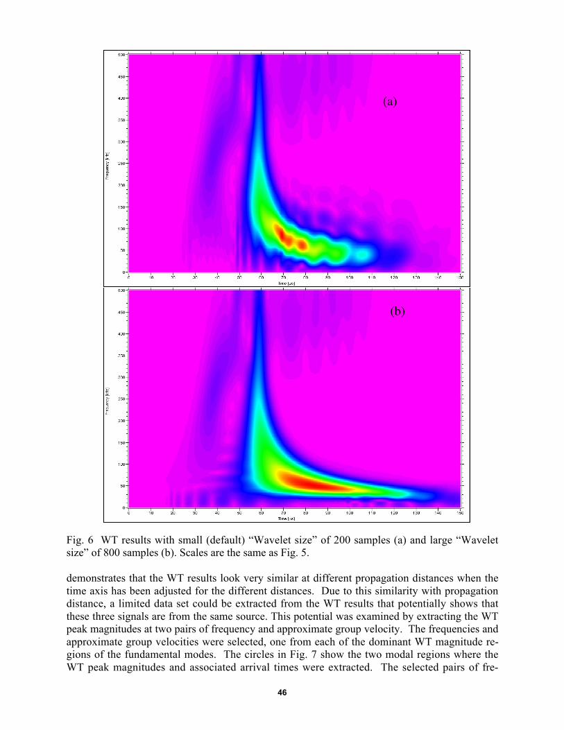
The �Wavelet size� has a default value of 200 samples. Figure 6 shows the WT results of thesame AE signal used for Fig. 5 with the default value (a) and a size value of 800 samples (b).For this figure the �Freq. Resolution� of 2 kHz was used along with a color factor of 1. It can beseen that the larger �Wavelet size� gives a smoother result. With a larger �Wavelet size� value,the calculation requires more time. To date, our observation has been that an increase in the�Wavelet size� is advisable when the larger amplitudes in the WT are at frequencies below about100 kHz. Thus, we conclude that it is worthwhile to enhance the resolution and smoothness ofthe WT results at the cost of slightly longer computational times. For example, on a modern per-sonal computer, the WT shown in Fig. 6 (a) took about 6 s and that shown in Fig. 6 (b) tookabout 18 s. When WT results were used to extract quantitative results, the parameters were se-lected to provide better resolution. In other cases lower resolution was used for more qualitativeresults.

45

Fig. 5 WT results with low �Frequency resolution� (default) of 10 kHz (a) and high �Frequencyresolution� of 2 kHz (b). Both results with a �Wavelet size� of 800 samples. Figures show fre-quency (0 to 500 kHz) versus time (0 to 150 µs).

5. Correlation of WTs with Source Type (Large Plate)

To begin to study source identification using the FEM database, we first focus on WT resultsof calculated AE signals at three different propagation distances from a single source. Figure 7shows the WT results (�Freq. Resolution� of 2 kHz, �Wavelet size� of 600 samples and CF = 1)at the three available distances for an in-plane dipole source (dipole forces are aligned with thedirection of propagation to the sensors) at a depth of 1.723 mm in a large plate. This figure

(a)

(b)

46

Fig. 6 WT results with small (default) �Wavelet size� of 200 samples (a) and large �Waveletsize� of 800 samples (b). Scales are the same as Fig. 5.

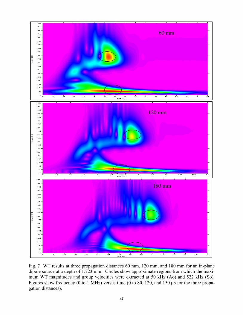
demonstrates that the WT results look very similar at different propagation distances when thetime axis has been adjusted for the different distances. Due to this similarity with propagationdistance, a limited data set could be extracted from the WT results that potentially shows thatthese three signals are from the same source. This potential was examined by extracting the WTpeak magnitudes at two pairs of frequency and approximate group velocity. The frequencies andapproximate group velocities were selected, one from each of the dominant WT magnitude re-gions of the fundamental modes. The circles in Fig. 7 show the two modal regions where theWT peak magnitudes and associated arrival times were extracted. The selected pairs of fre-

(b)

(a)

47

Fig. 7 WT results at three propagation distances 60 mm, 120 mm, and 180 mm for an in-planedipole source at a depth of 1.723 mm. Circles show approximate regions from which the maxi-mum WT magnitudes and group velocities were extracted at 50 kHz (Ao) and 522 kHz (So).Figures show frequency (0 to 1 MHz) versus time (0 to 80, 120, and 150 µs for the three propa-gation distances).

60 mm

120 mm

180 mm

48

Table 1. WT magnitudes (peak value) for specified mode and frequency at indicated group ve-locity for in-plane dipole source at a depth of 1.723 mm.

Propagation Indicated group WT Indicated group WT Magnitude ratio,distance, mm velocity, mm/µs Magnitude velocity, mm/µs Magnitude Ao/So

60 1.76 83,454 1.88 77,724 1.1120 2.02 58,265 1.86 45,904 1.3180 2.17 46,415 1.84 33,225 1.4

Ao mode at 50 kHz So mode at 522 kHz

Table 2. WT magnitudes (peak value) for specified mode and frequency at indicated group ve-locity with sources at a depth of 1.723 mm and a propagation distance of 180 mm.

Source Indicated group WT Indicated group WT Magnitude ratio,Type velocity, mm/µs Magnitude velocity, mm/µs Magnigude Ao/So

Out-of-plane 2.18 22,819 1.84 35,924 0.64In-plane 2.17 46,415 1.84 33,225 1.4

Crack initiation 2.14 34,603 1.83 14,546 2.4

Ao mode at 50 kHz So mode at 522 kHz

quency and group velocity were 50 kHz and about 2.16 mm/µs for the flexural mode (Ao) and522 kHz and about 1.84 mm/µs for the extensional mode (So). The extraction of the peak WTmagnitudes and their arrival times (in the approximate group-velocity region) was facilitated byan option that allows exporting the WT results into spreadsheets. Table 1 shows the extractedresults. The indicated group velocity was obtained by dividing the extracted arrival time into thepropagation distance from the source epicenter to the sensor location. Table 1 also shows theratios of the Ao/So peak WT magnitudes at the selected frequencies and group velocities. Theuse of such a ratio provides a measure that is independent of the original source strength.

Although the Ao/So ratio experiences an increase with increasing propagation distance, thischange could be corrected for by developing approximate rates of travel-distance attenuation ofthe WT magnitudes for the different modes and frequencies being used. Thus, it seems a limitedset of data can be extracted (from WT results) that indicates the same source was observed at dif-ferent propagation distances. However, it should be pointed out that the current dataset studiesonly the effect of propagation distance in one source-radiation direction (and the direction 180degrees opposed; a symmetrical direction). Since a source in a plate emits different amounts ofenergy of the bulk modes in different radiation directions, future research should check the aboveconclusions (for source identification) when the propagation distance varies along with the two-dimensional radiation direction in the plane of the plate. Due to the typical symmetries of radia-tion patterns of sources aligned with the plate coordinate axes, this check will need to be done foronly one quadrant rather than for a full 360 degrees.

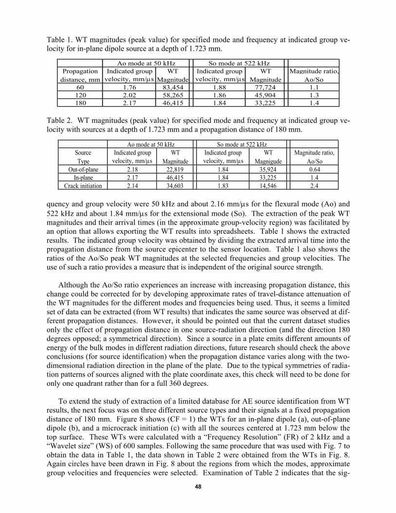
To extend the study of extraction of a limited database for AE source identification from WTresults, the next focus was on three different source types and their signals at a fixed propagationdistance of 180 mm. Figure 8 shows (CF = 1) the WTs for an in-plane dipole (a), out-of-planedipole (b), and a microcrack initiation (c) with all the sources centered at 1.723 mm below thetop surface. These WTs were calculated with a �Frequency Resolution� (FR) of 2 kHz and a�Wavelet size� (WS) of 600 samples. Following the same procedure that was used with Fig. 7 toobtain the data in Table 1, the data shown in Table 2 were obtained from the WTs in Fig. 8.Again circles have been drawn in Fig. 8 about the regions from which the modes, approximategroup velocities and frequencies were selected. Examination of Table 2 indicates that the sig-

49

Fig. 8. WT results from out-of-plane displacement signals for three different source types: (a)in-plane dipole, (b) out-of-plane dipole and (c) crack initiation. Sources are all at a depth of1.723 mm. Circles show approximate regions from which the maximum WT magnitudes andgroup velocities were extracted at 50 kHz (Ao) and 522 kHz (So). Figures show frequency (0 to1 MHz) versus time (0 to 150 µs) for the signals at 180 mm propagation distance.

nificant changes of the simple Ao/So ratio potentially could be used for source identification.The out-of-plane dipole source had the smallest ratio, and the crack-initiation source had thelargest ratio.

(b)

(c)

(a)

50

Fig. 9. WT plots as a function of the indicated source depths below the plate top surface. Thesource was an in-plane dipole with a 180 mm propagation distance. Figures show frequency (0to 1 MHz) versus time (0 to 150 µs).

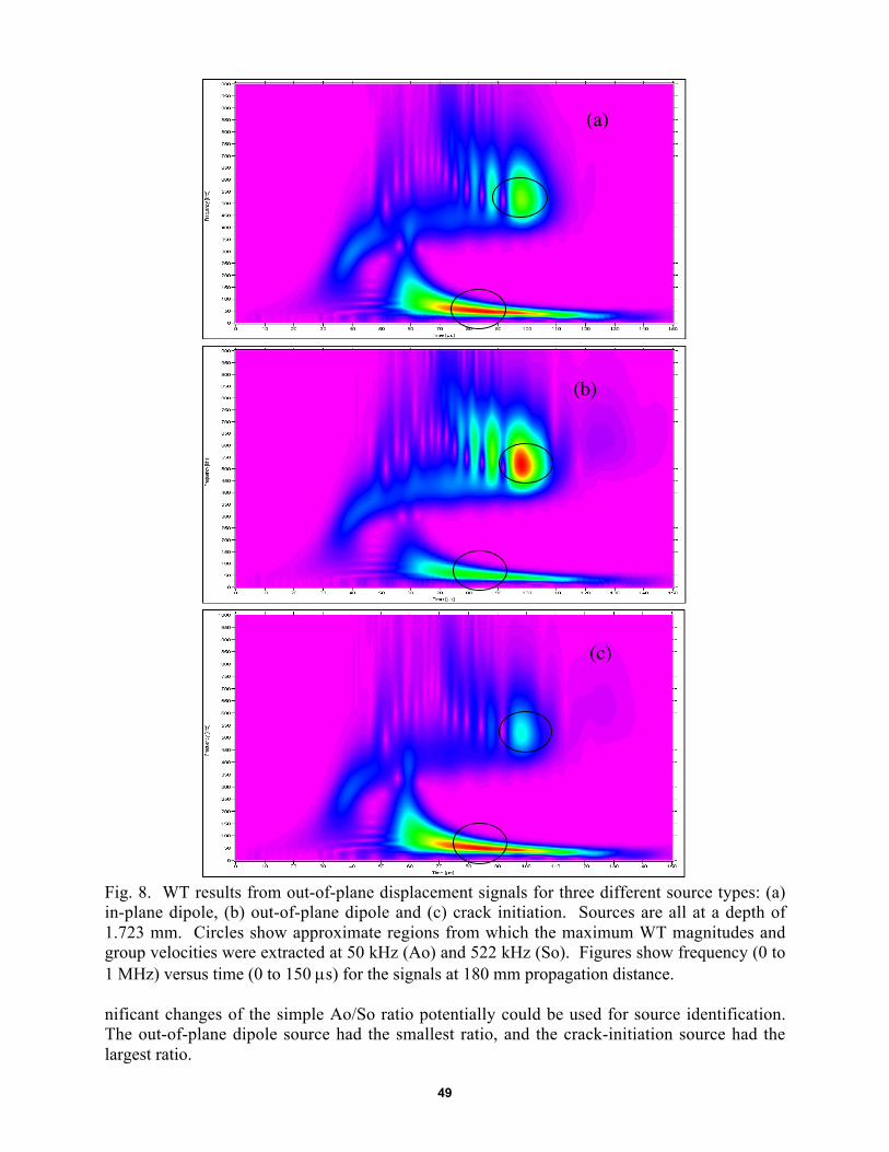
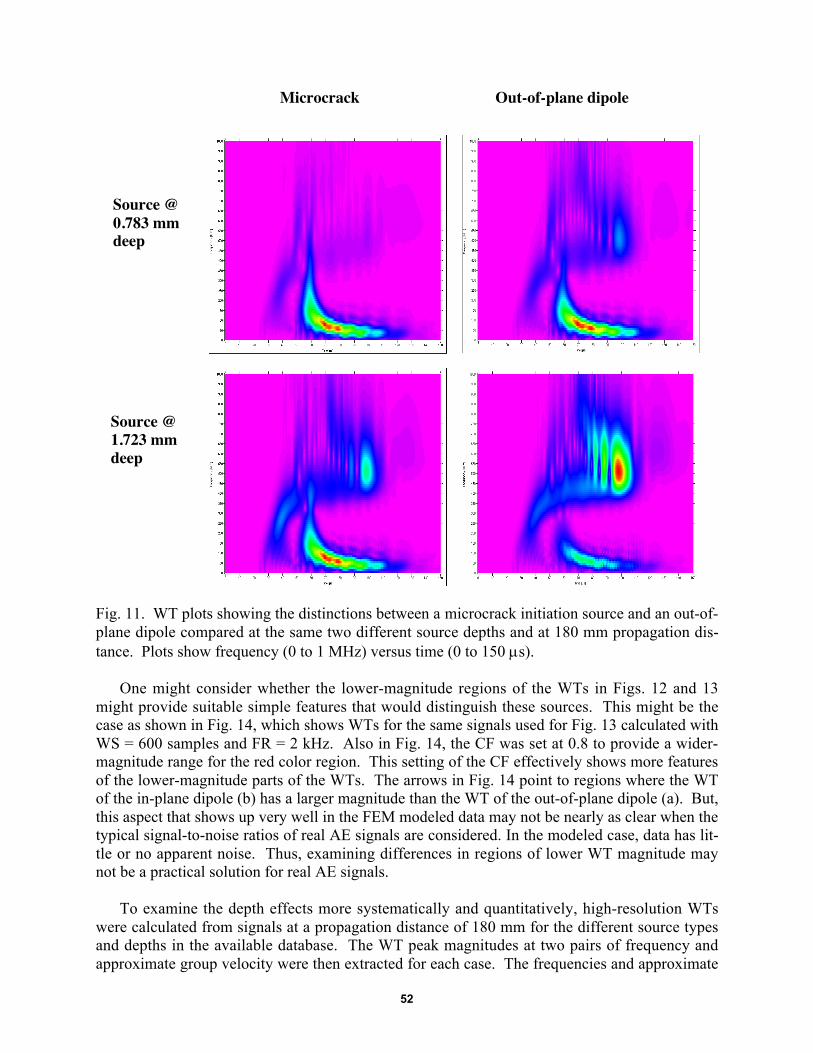
Examination of WT results for a single source type as a function of source depth revealssome potential difficulties in the approach suggested above. Figure 9 demonstrates the changesin WTs (with default values and CF = 1 for the AE signals at 180 mm) for an in-plane dipole as afunction of the depth of the source below the top surface of the plate. Even a casual examinationof the results in this figure shows that the WT result varies substantially as the depth of thesource changes. For the source located at the mid-plane (at 2.35 mm) the fundamental symmet-ric (extensional) mode dominates. As the source is moved closer to the surface, it is clear thatthe energy carried in the extensional mode decreases and most of the energy is carried in thefundamental anti-symmetric (flexural) mode. This dependence of the dominant Lamb modesand associated frequencies can also be seen in the signal waveforms and their FFTs. These re-sults are shown in Fig. 10 as a function of source depth for the same series of depths. The de-pendence of the WT results on source depth also is apparent for the out-of-plane dipole sourceand the more complicated microcrack initiation source. These WT results (default parametersand CF = 1) for the AE signals at 180 mm are shown in Fig. 11 for two different depths (0.783and 1.723 mm).

@ 2.037 mm

@ 1.723 mm

@ 1.41 mm

@ 1.097 mm

@ 0.47 mm

@ 2.35 mm, mid-plane

51

Fig. 10. Calculated AE signals with corresponding FFTs (in the same sequence top to bottom)for same cases shown in Fig. 9.

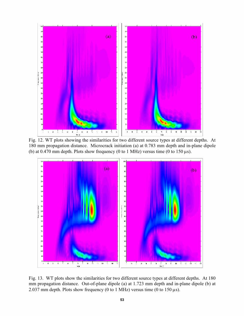
The possibility of extracting from WTs (of the out-of-plane displacement signals) a morelimited data set to uniquely identify the different AE sources certainly exists. However, it iscomplicated by the dependence of the AE signals and their WTs on the depth of the sources.There are two primary reasons for this complication. First, the Ao/So ratio changes not just withsource type but with source depth. The primary change (for the three source types considered)that takes place when the depth of a source changes is a transfer of more energy to either the ex-tensional mode or the flexural mode from the alternate mode. Thus, it does not seem possible toextract simple Ao/So ratio information, such as in Tables 1 and 2, from the WTs that is unique toa particular source type. Second, since at a fixed depth there are clear differences betweensource types (see Fig. 8 and Table 2), it is likely, as a consequence of the transfer of energy be-tween modes, that two different sources at two different source depths could have very similarWTs. This is in fact the case, as Figs. 12 and 13 show (calculated using default WT parameters)for signals at 180 mm from the sources. Figure 12 shows (CF = 1) that a microcrack initiationsource (a) at a depth of 0.783 mm has nearly the same WT as an in-plane dipole source (b) at adepth of 0.47 mm. Figure 13 demonstrates (CF = 1) the close WT similarities between an out-of-plane dipole source (a) at a depth of 1.723 mm and an in-plane dipole source (b) at a depth of2.037 mm.

-10

0

10

-10

0

10

-10

0

10

-10

0

10

-10

0

10

-10

0

10

20 50 80 110 140Time, µs

Dis

plac

emen

t, pm

Spec

tral

am

plitu

de, f

m

0

250

500

0

250

500

0

250

500

0

250500

0

250

500

0

250

500

0 0.2 0.4 0.6 0.8 1Frequency, MHz

@ 2.35 mm,mid-plane

@ 2.037 mm

@ 1.723 mm

@ 1.41 mm

@ 1.097 mm

@ 0.47 mm

52

Fig. 11. WT plots showing the distinctions between a microcrack initiation source and an out-of-plane dipole compared at the same two different source depths and at 180 mm propagation dis-tance. Plots show frequency (0 to 1 MHz) versus time (0 to 150 µs).

One might consider whether the lower-magnitude regions of the WTs in Figs. 12 and 13might provide suitable simple features that would distinguish these sources. This might be thecase as shown in Fig. 14, which shows WTs for the same signals used for Fig. 13 calculated withWS = 600 samples and FR = 2 kHz. Also in Fig. 14, the CF was set at 0.8 to provide a wider-magnitude range for the red color region. This setting of the CF effectively shows more featuresof the lower-magnitude parts of the WTs. The arrows in Fig. 14 point to regions where the WTof the in-plane dipole (b) has a larger magnitude than the WT of the out-of-plane dipole (a). But,this aspect that shows up very well in the FEM modeled data may not be nearly as clear when thetypical signal-to-noise ratios of real AE signals are considered. In the modeled case, data has lit-tle or no apparent noise. Thus, examining differences in regions of lower WT magnitude maynot be a practical solution for real AE signals.

To examine the depth effects more systematically and quantitatively, high-resolution WTswere calculated from signals at a propagation distance of 180 mm for the different source typesand depths in the available database. The WT peak magnitudes at two pairs of frequency andapproximate group velocity were then extracted for each case. The frequencies and approximate

Out-of-plane dipoleMicrocrack

Source @0.783 mmdeep

Source @1.723 mmdeep

53

Fig. 12. WT plots showing the similarities for two different source types at different depths. At180 mm propagation distance. Microcrack initiation (a) at 0.783 mm depth and in-plane dipole(b) at 0.470 mm depth. Plots show frequency (0 to 1 MHz) versus time (0 to 150 µs).

Fig. 13. WT plots show the similarities for two different source types at different depths. At 180mm propagation distance. Out-of-plane dipole (a) at 1.723 mm depth and in-plane dipole (b) at2.037 mm depth. Plots show frequency (0 to 1 MHz) versus time (0 to 150 µs).

(a) (b)

(a) (b)

54

Fig. 14. Same cases and scales as Fig. 13 with color factor changed to 0.8 to examine differ-ences in WTs in their lower magnitude regions. Arrows point to higher magnitude regions in thein-plane dipole (b) versus the out-of-plane dipole (a).

Fig. 15. Ao/So ratio of peak WT magnitudes versus AE source depth for the microcrack initia-tion, in-plane dipole and out-of-plane dipole sources at 180 mm propagation distance. Peakmagnitudes at 50 kHz and approximate group velocity of 2.16 mm/µs for Ao and at 522 kHz andapproximate group velocity of 1.84 mm/µs for So.

S14_2698

(a) S14_2729(b)

0.001

0.01

0.1

1

10

100

0 0.5 1 1.5 2 2.5Depth below surface, mm

WT

mag

nitu

de r

atio

A0/S

0

MicrocrackIn-plane dipole

Out-of-plane dipole

55

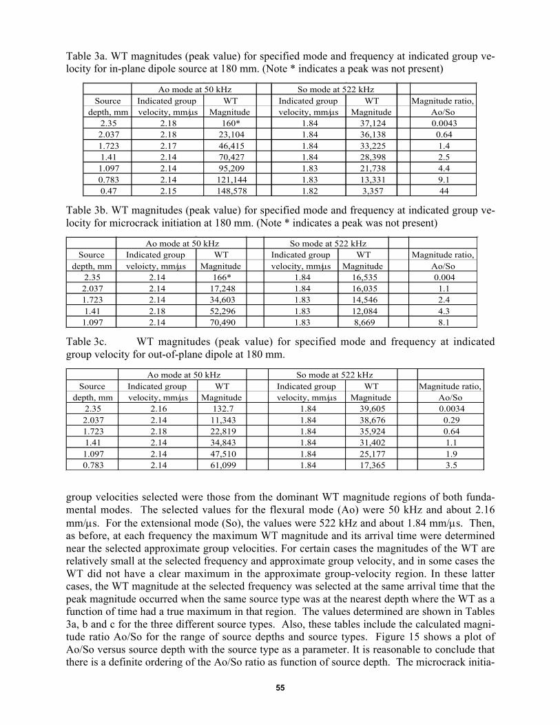
Table 3a. WT magnitudes (peak value) for specified mode and frequency at indicated group ve-locity for in-plane dipole source at 180 mm. (Note * indicates a peak was not present)

Source Indicated group WT Indicated group WT Magnitude ratio,depth, mm velocity, mm/µs Magnitude velocity, mm/µs Magnitude Ao/So

2.35 2.18 160* 1.84 37,124 0.00432.037 2.18 23,104 1.84 36,138 0.641.723 2.17 46,415 1.84 33,225 1.41.41 2.14 70,427 1.84 28,398 2.51.097 2.14 95,209 1.83 21,738 4.40.783 2.14 121,144 1.83 13,331 9.10.47 2.15 148,578 1.82 3,357 44

Ao mode at 50 kHz So mode at 522 kHz

Table 3b. WT magnitudes (peak value) for specified mode and frequency at indicated group ve-locity for microcrack initiation at 180 mm. (Note * indicates a peak was not present)

Source Indicated group WT Indicated group WT Magnitude ratio,depth, mm veloicty, mm/µs Magnitude velocity, mm/µs Magnitude Ao/So

2.35 2.14 166* 1.84 16,535 0.0042.037 2.14 17,248 1.84 16,035 1.11.723 2.14 34,603 1.83 14,546 2.41.41 2.18 52,296 1.83 12,084 4.31.097 2.14 70,490 1.83 8,669 8.1

Ao mode at 50 kHz So mode at 522 kHz

Table 3c. WT magnitudes (peak value) for specified mode and frequency at indicatedgroup velocity for out-of-plane dipole at 180 mm.

Source Indicated group WT Indicated group WT Magnitude ratio,depth, mm velocity, mm/µs Magnitude velocity, mm/µs Magnitude Ao/So

2.35 2.16 132.7 1.84 39,605 0.00342.037 2.14 11,343 1.84 38,676 0.291.723 2.18 22,819 1.84 35,924 0.641.41 2.14 34,843 1.84 31,402 1.11.097 2.14 47,510 1.84 25,177 1.90.783 2.14 61,099 1.84 17,365 3.5

Ao mode at 50 kHz So mode at 522 kHz

group velocities selected were those from the dominant WT magnitude regions of both funda-mental modes. The selected values for the flexural mode (Ao) were 50 kHz and about 2.16mm/µs. For the extensional mode (So), the values were 522 kHz and about 1.84 mm/µs. Then,as before, at each frequency the maximum WT magnitude and its arrival time were determinednear the selected approximate group velocities. For certain cases the magnitudes of the WT arerelatively small at the selected frequency and approximate group velocity, and in some cases theWT did not have a clear maximum in the approximate group-velocity region. In these lattercases, the WT magnitude at the selected frequency was selected at the same arrival time that thepeak magnitude occurred when the same source type was at the nearest depth where the WT as afunction of time had a true maximum in that region. The values determined are shown in Tables3a, b and c for the three different source types. Also, these tables include the calculated magni-tude ratio Ao/So for the range of source depths and source types. Figure 15 shows a plot ofAo/So versus source depth with the source type as a parameter. It is reasonable to conclude thatthere is a definite ordering of the Ao/So ratio as function of source depth. The microcrack initia-

56

tion source results in the highest values and the out-of-plane dipole has the lowest values, withthe in-plane dipole source in between. The relative differences between the ratios at a fixeddepth are not small, since the ratio scale in the figure is logarithmic. At the mid-plane depth (2.35mm), the ratio values are likely not reliable due to the very small WT magnitudes for the Aomode. Also, these Ao values were in most cases arbitrarily selected as described above since theAo mode did not have a peak value for the approximate group velocity region of the mode.

It is clear in the case of experimental data when the source depth is unknown that the Ao/Soratio alone will not uniquely define a source type. But, if one considers the data in Fig. 15 to bethat for a radiation direction of zero degrees, then it may be possible that results of Ao/So ratiosfrom other radiation directions could provide sufficient additional information to uniquely iden-tify the source type. This expectation, not unlike the approach of Buttle and Scruby (1990a),uses the fact that the radiation pattern is different for different source types. Since in experi-mental situations typically three or four sensors are hit when two-dimensional source location isdetermined (a prerequisite for the above approach, since the selected approximate group velocityneeds to be converted to an approximate arrival time), signals are typically available in severaltwo-dimensional radiation directions. For these different radiation directions, the Ao/So ratiocould be extracted from WTs of the signals. These ratios could then be compared as a functionof the radiation angle with modeled results of the Ao/So ratio versus radiation angle determinedfor different source types and depths. This method could possibly add sufficient information touniquely identify the source type and source depth. Based upon these observations in future re-search we expect to examine the above approach with a FEM database that includes other radia-tion directions.

The application to experimental AE data of the Ao/So ratio approach will likely experiencedifficulties when the source is located very near the plate surfaces or very near the plate�s mid-plane. As the first and last rows of Tables 3a, b and c show, in these cases either the Ao or SoWT-based magnitude is small, and they do not always have a local maximum (at a given fre-quency and associated approximate group velocity). Thus, for experimental data from sourcesnear the mid-plane, effects of low signal-to-noise ratios will likely eliminate the possibility ofcalculating meaningful Ao/So ratios. A possible solution to this problem might be to focus on thesingle dominant mode for these source-depth cases. For example, for a source located near or atthe mid-plane of the plate two or more frequencies and associated approximate group velocitiescould be selected from the So mode. At these frequencies and velocities the maximum magni-tudes of the WT could be determined within the So mode. Then ratios such as So (at 522 kHz)to So (at say 325 kHz) could be calculated. It is possible that this ratio or other appropriate onesmight result in distinguishing different source types located near the plate mid-plane. And for asource located near the plate surfaces, a ratio from two frequencies of the Ao mode could beused. Hence, in future research we expect to examine such an approach using the current FEMdatabase extended to include other source types, such as a shear source, and various radiationangles.

6. WT Data Subsets for Source Identification in Specimens with Nearby Edges

When the lateral size of the test specimen is decreased so that nearby edges are present, theAE signals and their WTs become much more complicated. This result is clearly seen in Fig. 16,which compares WTs of the AE signals (40 kHz high-pass) at 180 mm from in-plane and out-of-plane dipole sources in the small coupon specimen (Fig. 16(a)) and the large specimen (Fig.16(b)) both at a depth of 1.723 mm. Figure 17(a) also shows as a function of propagation dis-

57

Fig. 16. WT results (40 kHz high-pass AE signals) for coupon specimen (a) with multiple edgereflections compared to large specimen (b) without edge reflections. Results shown for an in-plane dipole source and an out-of-plane dipole source with a propagation distance of 180 mm.Sources centered at 1.723 mm below the top surface of the plate. Frequency (0 to 1 MHz) versustime (0 to 150 µs). Superimposed fundamental modes shown.

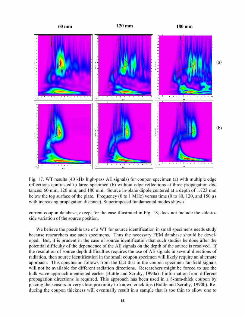
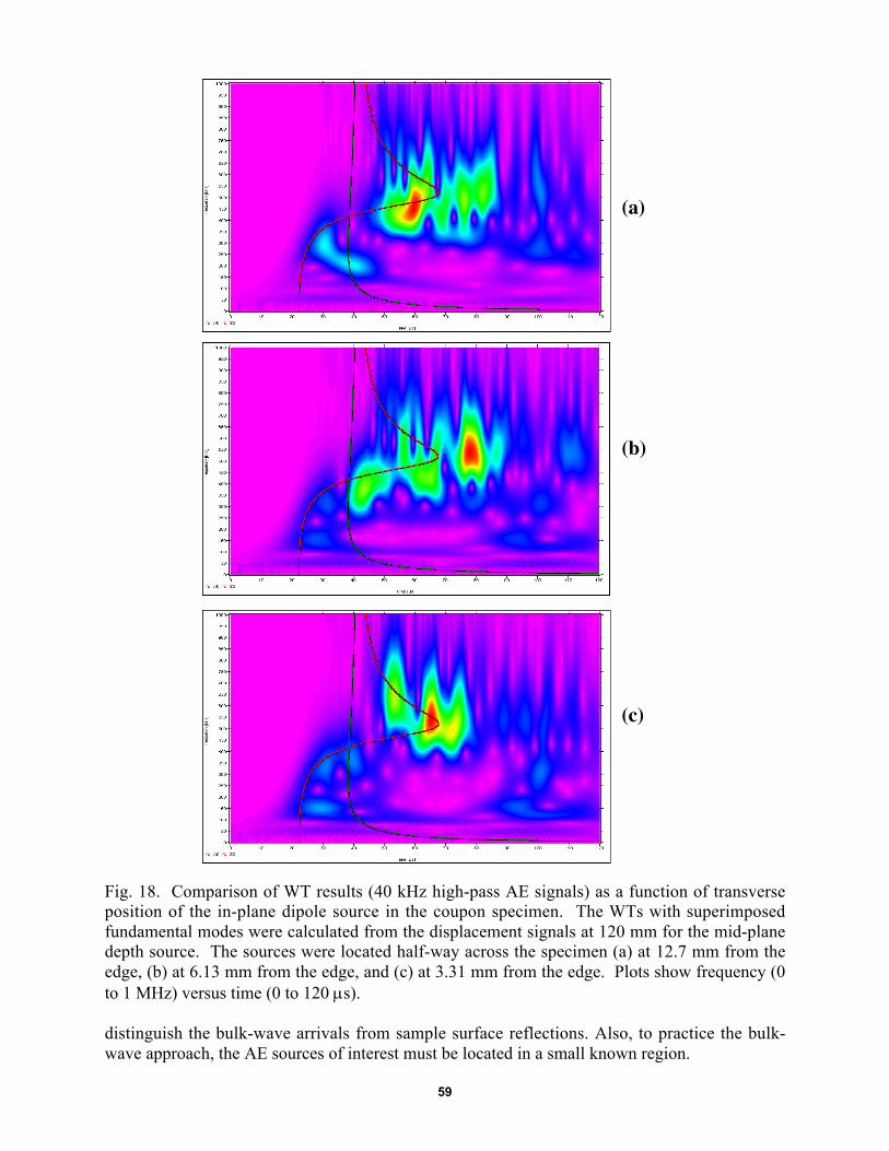
tance the significant distortion in the WT results (of AE signals from an in-plane dipole) for thecoupon specimen compared to the large specimen (Fig. 17(b)) with sources at a depth of 1.723mm. The distribution of signal energy in the coupon as shown in Figs. 16(a) and 17(a) does notclearly follow the shapes of the superimposed fundamental Lamb-mode curves from the disper-sion relations. Thus the extension of the possible extraction approaches proposed for sourceidentification in the large plate is not straightforward for the coupon specimen. Further, since thedistortion of the WT results is due to edge reflections (sides and at later times the specimenends), moving the source from side-to-side across the 25.4 mm dimension of the coupon speci-men will change the reflections in the AE signals. These source-position changes will alsochange the associated WTs as shown in Fig. 18 with superimposed fundamental modes. Thisfigure compares the WTs for in-plane dipole sources as a function of the transverse position ofthe AE source. In Fig. 18(a), the source was located half-way across the specimen at 12.7 mmfrom the coupon side edge. In Figs. 18(b) and 18(c), the source was successively at 6.13 mm and3.31 mm from the coupon side edge. The WTs (CF = 1, WS = 600) in these figures were calcu-lated from the AE signals at 180 mm from the sources. The source depth was 2.35 mm. The

In-plane dipole Out-of-plane dipole

(a)

(b)

58

Fig. 17. WT results (40 kHz high-pass AE signals) for coupon specimen (a) with multiple edgereflections contrasted to large specimen (b) without edge reflections at three propagation dis-tances: 60 mm, 120 mm, and 180 mm. Source in-plane dipole centered at a depth of 1.723 mmbelow the top surface of the plate. Frequency (0 to 1 MHz) versus time (0 to 80, 120, and 150 µswith increasing propagation distance). Superimposed fundamental modes shown

current coupon database, except for the case illustrated in Fig. 18, does not include the side-to-side variation of the source position.

We believe the possible use of a WT for source identification in small specimens needs studybecause researchers use such specimens. Thus the necessary FEM database should be devel-oped. But, it is prudent in the case of source identification that such studies be done after thepotential difficulty of the dependence of the AE signals on the depth of the source is resolved. Ifthe resolution of source depth difficulties requires the use of AE signals in several directions ofradiation, then source identification in the small coupon specimen will likely require an alternateapproach. This conclusion follows from the fact that in the coupon specimen far-field signalswill not be available for different radiation directions. Researchers might be forced to use thebulk wave approach mentioned earlier (Buttle and Scruby, 1990a) if information from differentpropagation directions is required. This approach has been used in a 8-mm-thick coupon byplacing the sensors in very close proximity to known crack tips (Buttle and Scruby, 1990b). Re-ducing the coupon thickness will eventually result in a sample that is too thin to allow one to

(a)

(b)

60 mm 120 mm 180 mm

59

Fig. 18. Comparison of WT results (40 kHz high-pass AE signals) as a function of transverseposition of the in-plane dipole source in the coupon specimen. The WTs with superimposedfundamental modes were calculated from the displacement signals at 120 mm for the mid-planedepth source. The sources were located half-way across the specimen (a) at 12.7 mm from theedge, (b) at 6.13 mm from the edge, and (c) at 3.31 mm from the edge. Plots show frequency (0to 1 MHz) versus time (0 to 120 µs).

distinguish the bulk-wave arrivals from sample surface reflections. Also, to practice the bulk-wave approach, the AE sources of interest must be located in a small known region.

(a)

(b)

(c)

60

7. Conclusions

A. Source Identification−Large Plates

! For the 4.7 mm aluminum plate thickness of the current FEM database, a potentially usefulparameter for source identification has been found. Using a separate selected frequency andapproximate group velocity for each fundamental mode, the WT coefficients (usually localmaxima for the frequency and group velocity) can be combined to form an Ao/So magnituderatio. This ratio was found to distinguish different source types when the sources were allcentered at the same depth below the plate surface and with the same propagation distance.

! But, since the values of this ratio overlap for different source types at different depths, it isnot possible to uniquely identify the source type with this small set of WT-based data.

! The current database indicates that the value ranking of the Ao/So magnitude ratio for differ-ent source types remains in the same order as a function of source depth. Since this result isfor a single radiation direction, it is to be expected that obtaining this ratio for other radiationdirections will supplement the WT-based data with possibly sufficient information touniquely classify the AE source type even with changing source depth. This expectation isbased upon the fact that different source types have different AE-energy radiation patterns.Thus a series of WT-based magnitude ratios from a total number, n, of different radiation an-gles (e.g., (Ao/So)1, (Ao/So)2, �, (Ao/So)n) could form an input vector to an artificial intelli-gence (AI) software program that would determine the AE source type. The AI programcould be initially trained using a FEM-generated database.

B. Source Identification−Small Coupon Specimens

! The inherent multiple edge reflections present in small coupon specimens complicate the useof WT coefficients for source identification. Since the current small coupon FEM databasedoes not include (except for one case) the important parameter (relative to edge reflection ef-fects) of changes in specimen side-to-side position of the source, the current database did notallow a full examination of these complications.

Acknowledgement

This work was partially supported by NASA Langley. We wish to express our gratitude toProf. Takemoto, who released the source code of the wavelet transform software his group haddeveloped and made AGU-Vallen Wavelet available. We also thank Dr. Y. Mizutani and Mr.Jochen Vallen for making the program into a highly usable form. Their contributions have sig-nificantly advanced the field of AE.

References

D. J. Buttle and C. B. Scruby, �Characterization of Fatigue of Aluminum Alloys by AcousticEmission, Part 1-Identification of Source Mechanism�, Journal of Acoustic Emission, 9, No. 4,1990a, 243-254.

D. J. Buttle and C. B. Scruby, �Characterization of Fatigue of Aluminum Alloys by AcousticEmission, Part II � Discrimination Between Primary and Secondary Emissions�, Journal ofAcoustic Emission, 9, No. 4, 1990b, 255-269.

61

Dawei Guo, Ajit K. Mal and Marvin A. Hamstad, �AE Wavefield Calculations in a Plate�, inProgress in Acoustic Emission IX, Acoustic Emission Working Group and Acoustic EmissionGroup, 1998, pp. IV-19 to IV-29.

M. A. Hamstad, A. O'Gallagher and J. Gary, "Modeling of Buried Acoustic Emission Monopoleand Dipole Sources With a Finite Element Technique", Journal of Acoustic Emission, 17, No. 3-4, 1999, 97-110.

R. L. Mehan and J.V. Mullin, �Analysis of Composite Failure Mechanisms Using AcousticEmissions�, Journal of Composite Materials, 5, April 1971, 266-269.

W. H. Prosser, M. A. Hamstad, J. Gary and A. O'Gallagher, "Reflections of AE Waves in FinitePlates: Finite Element Modeling and Experimental Measurements", Journal of Acoustic Emis-sion, 17, No. 1-2, 1999, 37-47.

H. Suzuki, T. Kinjo, Y. Hayashi, M. Takemoto and K. Ono, �Wavelet Transform of AcousticEmission Signals�, Journal of Acoustic Emission, 14, No. 2, 1996, 69-84.

M. Takemoto, H. Nishino and K. Ono, "Wavelet Transform - Applications to AE Signal Analy-sis", Acoustic Emission - Beyond the Millennium, Elsevier (2000), pp. 35-56.

Vallen-Systeme GmbH, Münich, Germany, http://www.vallen.de/wavelet/index.html, 2001.

R. Weaver and Y. H. Pao, �Axisymmetrical Waves Excited by a Point Source in a Plate�, Jour-nal of Applied Mechanics, 49, 1982a, 821-836.

R. Weaver and Y. H. Pao, �Spectra of Transient Waves in Elastic Plates�, Journal of the Acous-tical Society of America, 72, 1982b, 1933-1941.

H. Yamada, Y. Mizutani, H. Nishino, M. Takemoto and K. Ono, "Lamb Wave Source Locationof Impact on Anisotropic Plates", Journal of Acoustic Emission, 18, (2000, December), 51-60.