Embed Size (px)
Citation preview
University of Central Florida University of Central Florida
STARS STARS
Electronic Theses and Dissertations, 2004-2019
2012
Multi-vehicle Dispatching And Routing With Time Window Multi-vehicle Dispatching And Routing With Time Window
Constraints And Limited Dock Capacity Constraints And Limited Dock Capacity
Ahmed El-Nashar University of Central Florida
Part of the Industrial Engineering Commons
Find similar works at: https://stars.library.ucf.edu/etd
University of Central Florida Libraries http://library.ucf.edu
This Doctoral Dissertation (Open Access) is brought to you for free and open access by STARS. It has been accepted
for inclusion in Electronic Theses and Dissertations, 2004-2019 by an authorized administrator of STARS. For more
information, please contact [email protected].
STARS Citation STARS Citation El-Nashar, Ahmed, "Multi-vehicle Dispatching And Routing With Time Window Constraints And Limited Dock Capacity" (2012). Electronic Theses and Dissertations, 2004-2019. 2281. https://stars.library.ucf.edu/etd/2281
MULTI-VEHICLE DISPATCHING AND ROUTING WITH TIME WINDOW
CONSTRAINTS AND LIMITED DOCK CAPACITY
by
AHMED EL-NASHAR
B.S. Industrial Engineering, Arab Academy for Science and Technology, Egypt, 1999
M.S. Management Engineering, Arab Academy for Science and Technology, Egypt, 2006
M.S. Industrial Engineering, University of Central Florida, 2009
A dissertation submitted in partial fulfillment of the requirements
for the degree of Doctor of Philosophy
in the Department of Industrial Engineering and Management Systems
in the College of Engineering and Computer Science
at the University of Central Florida
Orlando, Florida
Fall Term
2012
Major Professor: Dima Nazzal

ii
ABSTRACT
The Vehicle Routing Problem with Time Windows (VRPTW) is an important and
computationally hard optimization problem frequently encountered in Scheduling and logistics.
The Vehicle Routing Problem (VRP) can be described as the problem of designing the most
efficient and economical routes from one depot to a set of customers using a limited number of
vehicles. This research addresses the VRPTW under the following additional complicating
features that are often encountered in practical problems:
1. Customers have strict time windows for receiving a vehicle, i.e., vehicles are not allowed
to arrive at the customer’s location earlier than the lower limit of the specified time
window, which is relaxed in previous research work.
2. There is a limited number of loading/unloading docks for dispatching/receiving the
vehicles at the depot
The main goal of this research is to propose a framework for solving the VRPTW with the
constraints stated above by generating near-optimal routes for the vehicles so as to minimize the
total traveling distance. First, the proposed framework clusters customers into groups based on
their proximity to each other. Second, a Probabilistic Route Generation (PRG) algorithm is
applied to each cluster to find the best route for visiting customers by each vehicle; multiple
routes per vehicle are generated and each route is associated with a set of feasible dispatching
times from the depot. Third, an assignment problem formulation determines the best dispatching
time and route for each vehicle that minimizes the total traveling distance.
iii
The proposed algorithm is tested on a set of benchmark problems that were originally developed
by Marius M. Solomon and the results indicate that the algorithm works well with about 1.14%
average deviation from the best-known solutions. The benchmark problems are then modified by
adjusting some of the customer time window limits, and adding the staggered vehicle dispatching
constraint. For demonstration purposes, the proposed clustering and PRG algorithms are then
applied to the modified benchmark problems.
iv
TABLE OF CONTENTS
LIST OF FIGURES ..................................................................................................................... viii
LIST OF TABLES .......................................................................................................................... x
CHAPTER 1: INTRODUCTION ............................................................................................. 1
1.1 Role of Distribution .......................................................................................................... 1
1.2 Vehicle Routing Problem Structure ................................................................................. 4
1.3 Problem Definition ........................................................................................................... 8
1.3.1 Problem Formulation .............................................................................................. 11
1.4 Research Objective ......................................................................................................... 16
CHAPTER 2: LITERATURE REVIEW ................................................................................ 18
2.1 Introduction .................................................................................................................... 18
2.2 Exact Algorithms............................................................................................................ 20
2.3 Classical Heuristics ........................................................................................................ 22
2.3.1 Sequential Route Construction Heuristics .............................................................. 22
2.3.2 Parallel Route Construction Heuristics ................................................................... 26
v
2.4 Meta-Heuristics .............................................................................................................. 28
2.4.1 Trajectory Methods ................................................................................................. 28
2.4.1.1 Tabu Search ..................................................................................................... 28
2.4.1.2 Simulated Annealing ....................................................................................... 31
2.4.1.3 Neighborhood Search Meta-Heuristics ........................................................... 33
2.4.2 Population Based Methods ..................................................................................... 36
2.4.2.1 Evolutionary Computation .............................................................................. 37
2.4.2.2 Ant Colony Optimization ................................................................................ 47
2.5 Summary and Research Gap .......................................................................................... 51
CHAPTER 3: PROPOSED METHODOLOGY FOR SOLVING VRPTW WITH LIMITED
DISPATCHING CAPACITY ....................................................................................................... 55
3.1 Proposed Solution Framework ....................................................................................... 55
3.2 Clustering Algorithm...................................................................................................... 56
3.2.1 The Mechanics of Clustering Algorithm ................................................................ 57
3.2.1.1 Determining the Acceptable Percent Increase in Route Length (R) ............... 60
3.3 Routing Algorithm ......................................................................................................... 61

vi
3.3.1 Introduction ............................................................................................................. 61
3.3.2 The Probabilistic Route Generation Algorithm ...................................................... 63
3.3.2.1 The Routes Table ............................................................................................. 64
3.3.2.2 The Frequency Table ....................................................................................... 65
3.3.2.3 The Probability Table ...................................................................................... 66
3.3.2.4 The Cumulative Probability Table .................................................................. 67
3.3.3 PRG Algorithm Mechanics ..................................................................................... 68
3.3.3.1 Algorithm Initialization ................................................................................... 70
3.3.3.2 PRG Algorithm Description ............................................................................ 70
3.3.4 Local Search............................................................................................................ 73
3.3.5 Assigning Dispatching Times ................................................................................. 74
CHAPTER 4: MODEL AND ALGORITHM VALIDATION .............................................. 78
4.1 Probabilistic Route Generation (PRG) Algorithm ......................................................... 78
4.1.1 Algorithm Convergence .......................................................................................... 78
4.1.2 Computational Results ............................................................................................ 79
4.2 VRPTW Benchmark Problems ...................................................................................... 83

vii
4.2.1 Computational Results ............................................................................................ 84
CHAPTER 5: VRPTW BENCHMAK PROBLEMS MODIFICATION AND TESTING .... 87
5.1 VRPTW Benchmark Problems Structure ....................................................................... 87
5.2 VRPTW Benchmark Problems Modification ................................................................ 89
5.2.1 Time Window Modification ................................................................................... 90
5.2.2 Staggered Vehicle Dispatching ............................................................................... 98
5.3 Vehicle Dispatching Time Assignment.......................................................................... 99
CHAPTER 6: RESEARCH SUMMARY AND FUTURE RESEARCH DIRECTIONS .... 105
6.1 Research Summary ....................................................................................................... 105
6.2 Research Contributions ................................................................................................ 106
6.3 Future Research Directions .......................................................................................... 107
REFERENCES ........................................................................................................................... 109
viii
LIST OF FIGURES
Figure 1: Transportation modes and its associated annual costs (Duych, 2008) ............................ 2
Figure 2: Traveling Salesperson Problem. ...................................................................................... 3
Figure 3: Vehicle Routing Problem. ............................................................................................... 4
Figure 4: Parameters, Constraints and Objectives of the VRP ....................................................... 5
Figure 5: Relations between different types of Vehicle Routing Problem (Toth and Vigo, 2002). 6
Figure 6: Schematic illustration of problem under study................................................................ 9
Figure 7: Effect of changing vehicle dispatching time on the time window constraints .............. 11
Figure 8 Summary of reviewed publications ................................................................................ 19
Figure 9: Swap Node and Swap Sequence mutation operators. ................................................... 44
Figure 10: Four steps of the proposed framework ........................................................................ 55
Figure 11: Customers clustered in groups. ................................................................................... 56
Figure 12: Clustering Algorithm ................................................................................................... 58
Figure 13: Pareto analysis for route increase percentages ............................................................ 60
Figure 14: Best sequence for visiting customers. ......................................................................... 61
ix
Figure 15: Simple illustration of routing algorithm. ..................................................................... 63
Figure 16: Generated Routes Table. ............................................................................................. 64
Figure 17: Frequency Counting Process ....................................................................................... 65
Figure 18: Probability Table Generation Process. ........................................................................ 67
Figure 19: Cumulative Probability Table ..................................................................................... 68
Figure 20: Flowchart showing the steps of the PRG algorithm .................................................... 69
Figure 21: Steps to construct route. .............................................................................................. 72
Figure 22: Applying local search algorithms to achieve better solutions ..................................... 74
Figure 23: Algorithm outcome...................................................................................................... 79
Figure 24: Time windows of Solomon’s tested benchmarking problems. ................................... 81
Figure 25: VRPTW benchmark problem structure ....................................................................... 88
Figure 26: VRPTW modification procedure................................................................................. 91
x
LIST OF TABLES
Table 1: Different approaches for solving VRPTW ..................................................................... 52
Table 2: Travel time per vehicle for dispatching time at 7:00 am ................................................ 75
Table 3: Vehicle travel times for different dispatching times from the depot .............................. 76
Table 4: Vehicle Loading, Dispatching and Dock Utilization. ..................................................... 76
Table 5: Travel time per vehicle for optimal dispatching time. .................................................... 77
Table 6: Results of executing PRG algorithm on a set of TSPTW benchmark problems ............ 82
Table 7: Results of applying the Clustering and PRG algorithms on a set of VRPTW benchmark
problems ........................................................................................................................................ 86
Table 8: Problem C101, 25 Customers ......................................................................................... 92
Table 9: Problem C101, 50 Customers ......................................................................................... 92
Table 10: Problem C103, 25 Customers ....................................................................................... 93
Table 11: Problem C103, 50 Customers ....................................................................................... 94
Table 12: Problem C107, 25 Customers ....................................................................................... 95
Table 13: Problem C107, 50 Customers ....................................................................................... 96
Table 14: Problem C109, 25 Customers ....................................................................................... 97
xi
Table 15: Problem C109, 50 Customers ....................................................................................... 97
Table 16: Travel distance for each cluster at different dispatching distance (Problem C107 – 50
customers) ..................................................................................................................................... 99
Table 17: Optimal vehicle dispatching time and total traveled distance (Problem C107 – 50
customers) ................................................................................................................................... 100
Table 18: Travel distance for each cluster at different dispatching distance (Problem C107 – 25
customers) ................................................................................................................................... 100
Table 19: Vehicle dispatching time and total traveling distance (Problem C107 – 25 customers)
..................................................................................................................................................... 100
Table 20: Traveling distance for each cluster at different dispatching distance (Problem C103 –
50 customers) .............................................................................................................................. 101
Table 21: Vehicle dispatching time and total traveled distance (Problem C103 – 50 customers)
..................................................................................................................................................... 101
Table 22: Traveling distance for each cluster at different dispatching distance (Problem C103 –
25 customers) .............................................................................................................................. 101
Table 23: Vehicle dispatching time and total traveled distance (Problem C103 – 25 customers)
..................................................................................................................................................... 102

xii
Table 24: Traveling distance for each cluster at different dispatching distance (Problem C101 –
50 customers) .............................................................................................................................. 102
Table 25: Vehicle dispatching time and total traveling distance (Problem C101 – 50 customers)
..................................................................................................................................................... 102
Table 26: Traveling distance for each cluster at different dispatching times (Problem C101 – 25
customers) ................................................................................................................................... 103
Table 27: Vehicle dispatching time and total traveling distance (Problem C101 – 25 customers)
..................................................................................................................................................... 104
1
CHAPTER 1: INTRODUCTION
1.1 Role of Distribution
Distribution is an important domain in our daily life, as it supports most social and economic
activities. Furthermore, it plays a key role in the fields of logistics and supply chains. Improving
operational efficiencies in distribution is receiving greater attention as fuel costs are continually
increasing. A small reduction in the traveled distance of a daily logistical operation directly
translates to cost reduction and decreased environmental impacts.
It has been estimated that distribution costs account for almost half of all logistics costs, and in
some industries, such as the food and beverage business, distribution costs can account for up to
70% of the value-added costs of the goods. In 1989, 76.5% of all transportation is by vehicles
(Backer et al., 1997; Golden and Wasil, 1987; Halse, 1992).
In 2007, it was estimated that American businesses made shipments valuing $11.8 trillion,
totaling 13 billion tons, and contributing 3.5 trillion ton-miles on the nation’s transportation
infrastructure, with 71% of these transportation operations carried out by truck (Duych, 2008).
Figure 1 summarizes the different mode of transportations and the associated annual costs for the
United States in 2007.

2
Figure 1: Transportation modes and its associated annual costs (Duych, 2008)
The importance of the distribution management mandates achieving high performance levels in
terms of the economic efficiency and service quality. The motivation to achieve economic
efficiency is exceptionally high in this competitive industry. A distribution firm’s main objective
is to make profit, while from a customer’s view (for a given level of quality) the major factor in
selecting a carrier is the cost
Further, lean manufacturing trends that target minimizing or eliminating inventory (just-in-time
procurement), and the need for quality control of the entire logistics chain driven by customer
demand and requirements impose a high service level. Such high levels can be achieved by
providing better total delivery time (be there fast), and reliable service (be there within specific
3
limits and be consistent in performance) (Crainic and Laporte, 1997).These and similar statistics
about the role of distribution in our society and the industry’s competitive nature propel the vast
body of research undertaken on traveling salesperson, vehicle routing and scheduling problems.
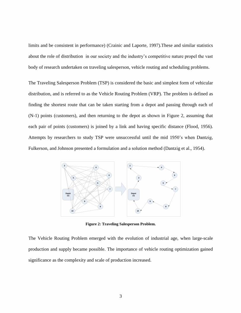
The Traveling Salesperson Problem (TSP) is considered the basic and simplest form of vehicular
distribution, and is referred to as the Vehicle Routing Problem (VRP). The problem is defined as
finding the shortest route that can be taken starting from a depot and passing through each of
(N-1) points (customers), and then returning to the depot as shown in Figure 2, assuming that
each pair of points (customers) is joined by a link and having specific distance (Flood, 1956).
Attempts by researchers to study TSP were unsuccessful until the mid 1950’s when Dantzig,
Fulkerson, and Johnson presented a formulation and a solution method (Dantzig et al., 1954).
Depot
(1)
2
5
10
7
6
4
3
9
8
Depot
(1)
2
5
10
7
6
4
3
9
8
Figure 2: Traveling Salesperson Problem.
The Vehicle Routing Problem emerged with the evolution of industrial age, when large-scale
production and supply became possible. The importance of vehicle routing optimization gained
significance as the complexity and scale of production increased.
4
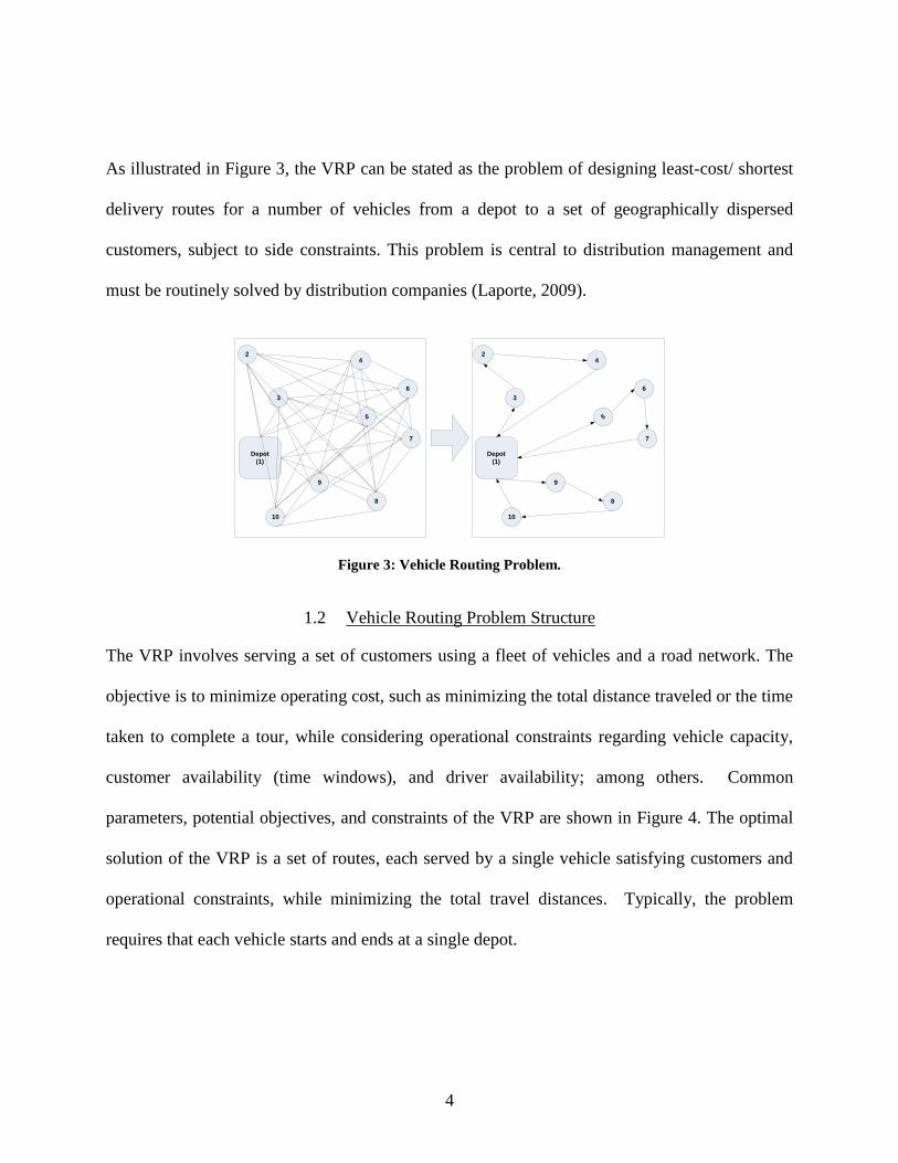
As illustrated in Figure 3, the VRP can be stated as the problem of designing least-cost/ shortest
delivery routes for a number of vehicles from a depot to a set of geographically dispersed
customers, subject to side constraints. This problem is central to distribution management and
must be routinely solved by distribution companies (Laporte, 2009).
Depot
(1)
2
5
10
7
6
4
3
9
8
Depot
(1)
2
5
10
7
6
4
3
9
8
Figure 3: Vehicle Routing Problem.
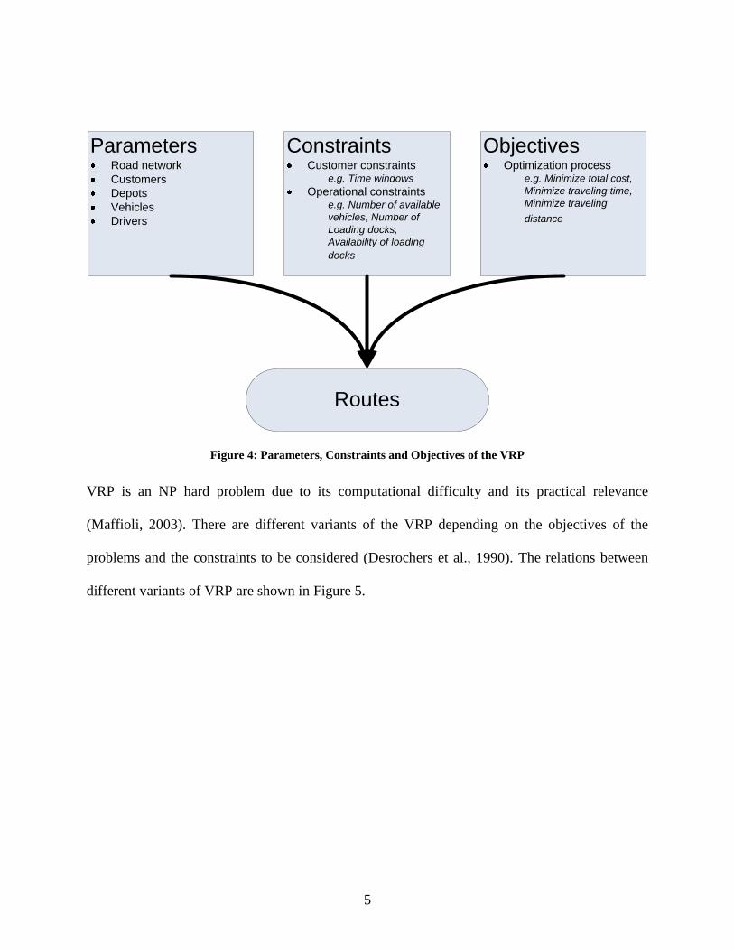
1.2 Vehicle Routing Problem Structure
The VRP involves serving a set of customers using a fleet of vehicles and a road network. The
objective is to minimize operating cost, such as minimizing the total distance traveled or the time
taken to complete a tour, while considering operational constraints regarding vehicle capacity,
customer availability (time windows), and driver availability; among others. Common
parameters, potential objectives, and constraints of the VRP are shown in Figure 4. The optimal
solution of the VRP is a set of routes, each served by a single vehicle satisfying customers and
operational constraints, while minimizing the total travel distances. Typically, the problem
requires that each vehicle starts and ends at a single depot.
5
ParametersRoad network
Customers
Depots
Vehicles
Drivers
ConstraintsCustomer constraints
e.g. Time windows
Operational constraintse.g. Number of available
vehicles, Number of
Loading docks,
Availability of loading
docks
ObjectivesOptimization process
e.g. Minimize total cost,
Minimize traveling time,
Minimize traveling
distance
Routes
Figure 4: Parameters, Constraints and Objectives of the VRP
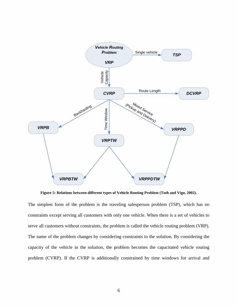
VRP is an NP hard problem due to its computational difficulty and its practical relevance
(Maffioli, 2003). There are different variants of the VRP depending on the objectives of the
problems and the constraints to be considered (Desrochers et al., 1990). The relations between
different variants of VRP are shown in Figure 5.
6
Vehicle Routing
Problem
VRP
TSP
VRPPDTWVRPBTW
VRPB
VRPTW
VRPPD
DCVRPCVRPRoute Length
Mixed Service
(Pickup and Delivery)
Tim
e W
ind
ow
Backhauling
Ve
hic
le
Ca
pa
city
Single vehicle
Figure 5: Relations between different types of Vehicle Routing Problem (Toth and Vigo, 2002).
The simplest form of the problem is the traveling salesperson problem (TSP), which has no
constraints except serving all customers with only one vehicle. When there is a set of vehicles to
serve all customers without constraints, the problem is called the vehicle routing problem (VRP).
The name of the problem changes by considering constraints to the solution. By considering the
capacity of the vehicle in the solution, the problem becomes the capacitated vehicle routing
problem (CVRP). If the CVRP is additionally constrained by time windows for arrival and
7
departure to and from customers, it is called the vehicle routing problem with time windows
(VRPTW).
The Vehicle Routing Problem with Pickup and Delivery (VRPPD), another extension of the
classical VRP, occurs when a number of goods are moved from a certain pickup location to a
certain delivery location. The objective is to identify the optimal routes to visit the pickup and
delivery locations. The Vehicle Routing Problem with Backhauls (VRPB) is considered a special
case of VRPPD in which there are two separate sets of customers: a set of customers to whom
products are delivered, and a set of vendors whose goods need to be transported back to the
distribution center; the main constraint in this type of problem is that all deliveries must be made
before any pickups. When there are limitations on vehicle capacity and the maximum route
distance, the problem is called the Distance Constrained Capacitated Vehicle Routing Problem
(DCVRP) (Toth and Vigo, 2002).
This research proposes a new algorithm for solving the VRPTW with additional constraints due
to the necessity to stagger the vehicles’ dispatching times from the depot or the vehicles’
receiving time at the depot due to, for example, a limited number of loading docks and/or
dispatching times.
The problem is decomposed into several sub-problems as is discussed in CHAPTER 3:. New
heuristics are developed to efficiently generate near-optimal schedules and routes. Section 1.3
presents the problem definition including the unique features studied in this research
investigation.
8
1.3 Problem Definition
The VRPTW problem has been studied extensively during the last decade, and researchers have
proposed different algorithms and heuristics for solving this problem. Most of the proposed
algorithms, however, ignore the lower bound of customers’ time windows. More specifically,
most of the proposed algorithms and heuristics allow the vehicle to wait at a customer’s premises
if the vehicle arrives before the start of the customer’s specified time window. Further, these
algorithms assume that all vehicles can be dispatched from the depot at the same time, which
might not be realistic in some practical situations, e.g., the depot might have a limited number of
dispatching/receiving docks.
In this research a new variant of the VRPTW has been studied, by adding two additional features
(constraints):
1. The vehicle schedule must satisfy both a lower limit and an upper limit of the
arrival time to customer . Therefore, vehicles are not allowed to wait at the customer
upon early arrival.
2. There is a limit on the number of vehicles that can be dispatched simultaneously from the
depot. This limit depends on the number of available docks (d) at the depot.
9
Represent
customers
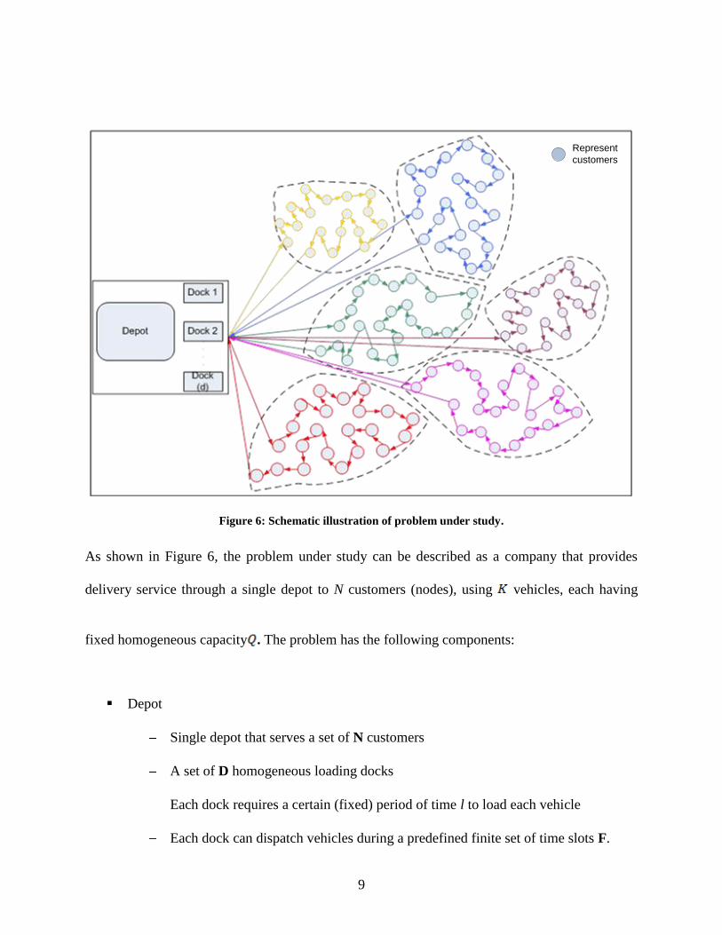
Figure 6: Schematic illustration of problem under study.
As shown in Figure 6, the problem under study can be described as a company that provides
delivery service through a single depot to N customers (nodes), using vehicles, each having
fixed homogeneous capacity . The problem has the following components:
Depot
Single depot that serves a set of N customers
A set of D homogeneous loading docks
Each dock requires a certain (fixed) period of time l to load each vehicle
Each dock can dispatch vehicles during a predefined finite set of time slots F.
10
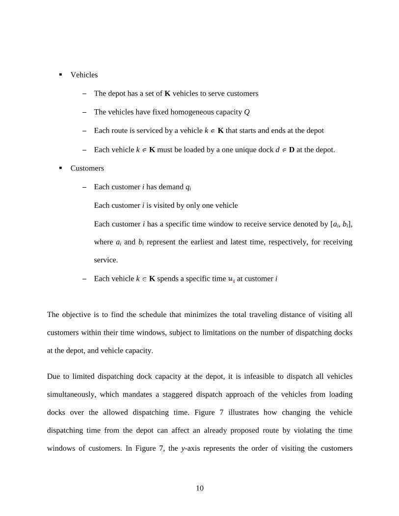
Vehicles
The depot has a set of K vehicles to serve customers
The vehicles have fixed homogeneous capacity Q
Each route is serviced by a vehicle k K that starts and ends at the depot
Each vehicle k K must be loaded by a one unique dock d D at the depot.
Customers
Each customer i has demand qi
Each customer i is visited by only one vehicle
Each customer i has a specific time window to receive service denoted by [ai, bi],
where ai and bi represent the earliest and latest time, respectively, for receiving
service.
Each vehicle k K spends a specific time at customer i
The objective is to find the schedule that minimizes the total traveling distance of visiting all
customers within their time windows, subject to limitations on the number of dispatching docks
at the depot, and vehicle capacity.
Due to limited dispatching dock capacity at the depot, it is infeasible to dispatch all vehicles
simultaneously, which mandates a staggered dispatch approach of the vehicles from loading
docks over the allowed dispatching time. Figure 7 illustrates how changing the vehicle
dispatching time from the depot can affect an already proposed route by violating the time
windows of customers. In Figure 7, the y-axis represents the order of visiting the customers

11
starting from the depot in the top of the y-axis and ending at the depot at the bottom of the y-axis.
The horizontal line represents the service time at customer’s location, while the declined line
represent the traveling time from one customer to another. The solid line represents dispatching
the vehicle from the depot at the appropriate time and how it meets all customers’ time windows,
while the dotted line shows how the customers’ time windows might be violated if the
dispatching time of the vehicle from the depot changed.
Time windows
violation
Time
Customer
time window
Depot
Depot
Dis
pa
tch
ing
tim
e fro
m
the
De
po
t
Dis
pa
tch
ing
tim
e fro
m
the
De
po
t
Arrival time at
customer (c)Departure time at
customer (c)
Start of time
window
End of time
window
Customer time window
Traveling time
Service time
Dispatching from depot
in appropriate time
Delaying dispatching
time from depot
Figure 7: Effect of changing vehicle dispatching time on the time window constraints
1.3.1 Problem Formulation
The problem can be considered a graph G = (N, A) with a set of N nodes representing the
customers and a set A of arcs with arc (i,j) A connecting node i to node j; the depot is
presented by Nodes 0 and (N + 1). A is the set of arcs that connect the different nodes. For each
12
arc (i,j) A, i j, there is a nonnegative cost cij that represents the travel distance between nodes
i and j in the network.
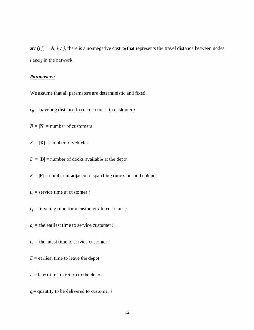
Parameters:
We assume that all parameters are deterministic and fixed.
cij = traveling distance from customer i to customer j
N = |N| = number of customers
K = |K| = number of vehicles
D = |D| = number of docks available at the depot
F = |F| = number of adjacent dispatching time slots at the depot
ui = service time at customer i
tij = traveling time from customer i to customer j
ai = the earliest time to service customer i
bi = the latest time to service customer i
E = earliest time to leave the depot
L = latest time to return to the depot
qi= quantity to be delivered to customer i
13
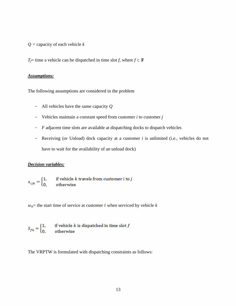
Q = capacity of each vehicle k
Tf= time a vehicle can be dispatched in time slot f, where f F
Assumptions:
The following assumptions are considered in the problem
All vehicles have the same capacity Q
Vehicles maintain a constant speed from customer i to customer j
F adjacent time slots are available at dispatching docks to dispatch vehicles
Receiving (or Unload) dock capacity at a customer i is unlimited (i.e., vehicles do not
have to wait for the availability of an unload dock)
Decision variables:
wik= the start time of service at customer when serviced by vehicle k
The VRPTW is formulated with dispatching constraints as follows:

14
s.t.
(1)
(2)
(3)
(4)
(5)
(6)
(7)

15
(8)
(9)
(10)
(11)
(12)
(13)
In the mathematical model, constraints (1) to (9) are those presented by Toth and Vigo (Toth and
Vigo, 2002) to formulate the VRPTW, and constraints (10) to (13) are the additional constraints
required for the staggered dispatching feature of the problem.
The objective is to minimize the total travel distance. Constraint (1) restricts the assignment of
each customer to exactly one vehicle. While constraints sets (2)-(4) characterize the flow on the
path to be followed by vehicle k. Constraints sets (5)-(7) and (8) guarantee schedule feasibility
with respect to time windows and vehicle capacity limitations, respectively. Constraint (10)
restricts the dispatching time of any of the vehicles to one of the available F dispatching time
16
slots. While constraint (11) ensures that one and only one dispatching time period f will be
assigned to each vehicle. Finally, constraint (12) ensures that the number of vehicles that can be
dispatched in a given time slot is less than or equal to the number of the available docks.
As previously mentioned, the VRP is NP hard due to its computational difficulty (Maffioli,
2003). Adding the constraints of time windows and the limited capacity of dispatching docks
increase the complexity of the problem and make it very difficult to solve in polynomial time.
Therefore, it follows that the VRPTW with limited dock capacity is also in the class of NP.
1.4 Research Objective
The goal of this research is to propose a solution framework for the VRPTW problem with
limited dispatching capacity constraint that generates a vehicle dispatching schedule for the
depot in order to minimize the total vehicle traveling distance. The following steps are taken in
order to develop this framework for solving the problem under study.
1. Propose a clustering approach that partitions the customers into subgroups considering the
proximity between customers and simultaneously satisfying the customers’ time window
constraints;
2. Propose an optimization procedure that produces near-optimal vehicle routes for each cluster
considering the upper and lower bounds of time windows for each customer and the limited
number of loading docks at the depot; and
3. Evaluate the proposed solution framework against benchmark problems via a computational
study.
17
As by-product of this research, a dock schedule can be developed compatible with the optimal
routing of vehicles.
Due to the vast body of literature on VRP, the literature review in Chapter 2 chiefly focuses on
the Vehicle Routing Problem with Time Windows and its variants, because it is the closest
representation to the problem under investigation in this research. Chapter 3 illustrates the details
of the research methodology and discusses the proposed algorithms for solving the research
problem. Chapter 4 presents the results of testing the performance of the proposed algorithms
and discusses the obtained results. Chapter 5 discusses the modification of VRPTW benchmark
problems and applies the proposed algorithms on the modified benchmark problems.
18
CHAPTER 2: LITERATURE REVIEW
2.1 Introduction
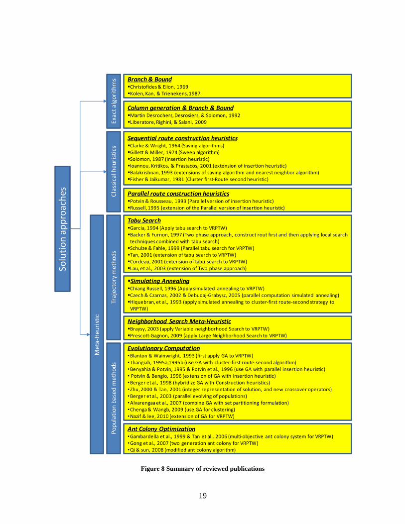
Due to the importance and wide applicability of the VRP, it is continuously investigated to
enhance existing algorithms and develop new exact algorithms and heuristics to achieve better
solutions in a reasonable time. Numerous researchers discuss the VRPTW and propose different
approaches for solving it. They propose three main approaches: Exact Algorithms, Heuristics, or
Metaheuristics. Figure 8 summarizes existing research on the VRPTW.
19
Exa
ct a
lgo
rith
ms
Cla
ssic
al h
eu
rist
ics
Me
ta-H
eu
rist
ic
Solv
ing
Ap
pro
ach
es
Branch & BoundChristofides & Eilon, 1969Kolen, Kan, & Trienekens, 1987
Column generation & Branch & BoundMartin Desrochers, Desrosiers, & Solomon, 1992Liberatore, Righini, & Salani, 2009
Sequential route construction heuristicsClarke & Wright, 1964 (Saving algorithms)Gillett & Miller, 1974 (Sweep algorithm)Solomon, 1987 (insertion heuristic) Ioannou, Kritikos, & Prastacos, 2001 (extension of insertion heuristic)Balakrishnan, 1993 (extensions of saving algorithm and nearest neighbor algorithm)Fisher & Jaikumar, 1981 (Cluster first-Route second heuristic)
Parallel route construction heuristicsPotvin & Rousseau, 1993 (Parallel version of insertion heuristic)Russell, 1995 (extension of the Parallel version of insertion heuristic)
Tabu SearchGarcia, 1994 (Apply tabu search to VRPTW)Backer & Furnon, 1997 (Two phase approach, construct rout first and then applying local search
techniques combined with tabu search)Schulze & Fahle, 1999 (Parallel tabu search for VRPTW)Tan, 2001 (extension of tabu search to VRPTW)Cordeau, 2001 (extension of tabu search to VRPTW)Lau, et al., 2003 (extension of Two phase approach)
Simulating AnnealingChiang Russell, 1996 (Apply simulated annealing to VRPTW)Czech & Czarnas, 2002 & Debudaj-Grabysz, 2005 (parallel computation simulated annealing)Hiquebran, et al., 1993 (apply simulated annealing to cluster-first route-second strategy to
VRPTW)
Neighborhood Search Meta-HeuristicBraysy, 2003 (apply Variable neighborhood Search to VRPTW)Prescott-Gagnon, 2009 (apply Large Neighborhood Search to VRPTW)
Evolutionary Computation•Blanton & Wainwright, 1993 (first apply GA to VRPTW)•Thangiah, 1995a,1995b (use GA with cluster-first route-second algorithm)•Benyahia & Potvin, 1995 & Potvin et al., 1996 (use GA with parallel insertion heuristic)• Potvin & Bengio, 1996 (extension of GA with insertion heuristic)•Berger et al., 1998 (hybridize GA with Construction heuristics)•Zhu, 2000 & Tan, 2001 (integer representation of solution, and new crossover operators) •Berger et al., 2003 (parallel evolving of populations)•Alvarengaa et al., 2007 (combine GA with set partitioning formulation)•Chenga & Wangb, 2009 (use GA for clustering)•Nazif & lee, 2010 (extension of GA for VRPTW)
Ant Colony Optimization•Gambardella et al., 1999 & Tan et al., 2006 (multi-objective ant colony system for VRPTW)•Gong et al., 2007 (two generation ant colony for VRPTW)•Qi & sun, 2008 (modified ant colony algorithm)
Tra
ject
ory
me
tho
ds
Po
pu
lati
on
ba
sed
me
tho
ds
Solu
tio
n a
pp
roac
hes
Figure 8 Summary of reviewed publications
20
2.2 Exact Algorithms
Over the last four decades, extensive research in the field of VRP proposes exact solution
algorithms. These algorithms range from basic branch-and-bound schemes to highly
sophisticated mathematical programs.
An Algorithm for the Vehicle Dispatching Problem proposed by Christofides & Eilon (1969) is
considered one of the first known branch-and-bound algorithms , the authors propose to add m-1
artificial depots to the graph and setting the distance between those artificial depots to infinity.
By adding those artificial depots the problem changes from VRP to TSP, this new problem is
called m-TSP. Each new TSP is solved by branching on arcs as proposed by Little et al. (1963).
Christofides & Eilon (1969) claim that they can improve the results of the Little et al. algorithm
by determining the lower bound of the traveling salesperson tour by calculating the minimal
spanning tree.
Kolen et al. (1987) propose a branch-and-bound method for VRPTW. The authors state that they
propose the first optimization method for VRPTW. The proposed branch-and-bound algorithm is
based on a branching rule, in which each node in the search tree corresponds to: (1) a set of fixed
routes that start and end at the depot, (2) a partial route starting at the depot, and (3) a set of
customers that are forbidden to be the next route stop. Initially, the fixed routes and the set of
forbidden customers are empty, while the partial route consists only of the depot. In the
branching process the algorithm starts with a customer who does not appear in any fixed or
partial route and is not forbidden. A lower bound is calculated at each node of the search tree for
21
the possible feasible extensions of the partial route by relaxing the constraint that forces each
customer not being served yet to be visited only once.
Desrochers et al. (1992) propose an algorithm that considers hard time windows; the time
windows of any of the customers can not be violated. For example, a vehicle waits at the
customer’s location, if it arrives earlier than the customer’s specified time window. Such case is
applicable in the fields of bank deliveries, postal deliveries, industrial refusal collection and bus
routing and scheduling. In this paper, the authors use column generation approach in conjunction
with branch-and-bound to generate an optimal solution.
Liberatore (2009) proposes an exact algorithm for solving the vehicle routing problem with soft
time windows (VRPSTW) using column generation method. Soft time windows are not
considered as constraints, but as preferences on the time of visiting the customer’s location. If a
customer is visited out of the preferred time window, a penalty is incurred in terms of additional
costs that are added to the total cost of the route rather than considering it a time window
violation. The main advantage of routing with soft time windows is that more stops can be added
to routes than in the case of hard time windows. The authors propose an algorithm that solves
VRPSTW as a resource constrained elementary shortest path problem with soft time windows,
which forms the basis to develop a branch-and-price algorithm for the exact optimization of the
VRPSTW.
The concept of the VRP is simple and easy to understand, and from the first impression we may
think that it is very easy to get an optimal solution for it. However, the problem is very complex,
and time consuming to reach an optimal solution and is considered NP-hard problem. Further,

22
adding constraints to the problem will increase its complexity. Christofides and Eilon (1969) and
Lenstra and Kan (1981) have shown that the vehicle routing problem is an NP-hard problem, and
consequently we can consider vehicle routing problem with time windows as an NP-hard
problem.
The work done by Savelsbergh (1985) and Solomon (1986) show that adding the time window
constraint to the vehicle routing problem increases the complexity of the problem and the
difficulty of reaching an optimal solution, and consequently reaching an optimal solution within
polynomial time is not expected.
2.3 Classical Heuristics
Heuristics may be considered as successful alternatives to provide promising solutions for
practical (realistic) size problems in reasonable computational time and requirement, but their
main limitation is the quality of the solution (Koskosidis et al., 1992), and the optimality gap.
2.3.1 Sequential Route Construction Heuristics
Clarke and Wright (1964) propose the saving algorithm. The algorithm starts by developing one
tour from the depot to each customer and back to the depot. The number of initial tours will be
equal to the number of customers. After setting the initial tours we start combining the different
tours together in order to reduce the total traveled distance. In order to determine the tours that
should be combined together, the saving that results from combining any two tours together (Sij)
are calculated, by adding distance from the depot to customer i (di0) and distance from the depot
to customer j (d0j) and subtracting from them the distance from customer i to customer j (dij).

23
After calculating the savings we rank them and list them in descending order of magnitude, and
we start joining tours together in such way that maximizes the savings. We keep combining tours
together until all customers are assigned to routes. The number of vehicles used in the solution is
an output of the algorithm. Gaskell (1967), Yellow (1970) and Paessens (1988) have also
proposed a number of variants of this method.
Gillett and Miller (1974) propose a heuristic algorithm, named the sweep algorithm for solving
medium and large scale vehicle routing problem with load and distance constraint for each
vehicle. The sweep algorithm divides the locations into a number of routes and then operates on
the individual routes until an optimum or near optimum solution is obtained. The authors state
that when the problem is broken down into a number of smaller sub-problems, the computation
time required for reaching the optimal solution increases somewhat in a linear, rather than, in an
exponential manner as more locations are added to a given problem. The sweep algorithm
consists mainly of two parts: a forward sweep and backward sweep. In the forward sweep,
locations are added to the route according to their polar-coordinate angle from the depot, the
locations with smaller polar-coordinate angles are added first to the route until the vehicle
capacity or distance constraint is reached. When the vehicle capacity or the distance constraint is
reached a new route is started. This process is repeated until all locations are assigned to routes.
In order to check if there is better solution that can be reached, a replacement process takes place
between consecutive routes by replacing the locations that are near to each other in the
consecutive routes. The replacement process takes place only if the total distance of the routes is
decreased. The backward sweep is similar to the forward sweep, except that the backward sweep
uses the locations with larger polar-coordinate angle from the depot to be added first to the
24
routes, and also the replacement process takes place between the constructed routes to check any
further improvement. The authors state that forward and backward sweep algorithms produce
different routes, and the smallest output of these two algorithms is considered the best solution.
Solomon (1987) propose a set of heuristics for solving the vehicle routing problem with time
windows. The first heuristic is an extension of the saving heuristic proposed by Clarke and
Wright (1964). The main savings algorithm is extended by considering the time window, and
consequently the route orientation becomes a very important issue to satisfy customer
requirements, as changing customers visiting sequence may affect satisfying customers’ time
windows. The second heuristic is a time-oriented nearest neighbor, in this algorithm the route
construction process starts by finding the closest customer to the depot that is not assigned to a
route yet, and then the heuristic searches among the feasible customers (with respect to time
windows, vehicle arrival time at the depot, and vehicle capacity constraint) for the closest one to
the last customer added to the route and adds it at the end of the route. A new route is started
whenever the heuristic fails to find a feasible insertion, unless there are no more customers left.
The third heuristic is the insertion heuristic; route construction in this heuristic is initialized with
a “seed” customer and the remaining un-routed customers are added into the route until an
operating constraint is violated. The seed customers are selected by finding either the farthest un-
routed customers from the depot or the un-routed customer with the lowest allowed starting time
for service. After initializing the route with a seed customer, the heuristic uses two criteria,
c1(i,u,j) and c2(i,u,j), to select customer u for insertion between customers i and j in the current
route. The first criteria c1(i,u,j)finds the insertion that minimizes the cost, while the second
criteria c2(i,u,j) finds the best position for the nominated insertion to provide the optimal feasible
25
solution (inserting a new insertion would affect the time of starting service in the successive
customers). The fourth heuristic is called “A Time-Oriented Sweep Heuristic”; this heuristic is
based on the idea of decomposing the problem into a clustering phase and a scheduling phase. In
the clustering phase, customers are assigned to vehicles as in the original sweep heuristic
proposed by Gillett and Miller (1974). In the scheduling phase a one-vehicle schedule is created
for the customers assigned to the vehicle, using a tour building heuristic like the insertion
heuristic.
Ioannou et al. (2001) propose a heuristic for solving the VRPTW, this heuristic is considered a
route construction sequential approach as it builds vehicle routes, one at a time. The proposed
heuristic is based on the generic insertion framework proposed by Solomon (1987). After
initializing a route with a ‘seed’ customer the heuristic uses two criteria to insert a new customer
to that route. The first criterion selects the best customer to be inserted in the current route, while
the second criterion determines the best place that the selected customer can be inserted in the
current route. This heuristic is based on the minimization function of the greedy look-ahead
solution approach of Atkinson (1994); the basic idea of the new selection and insertion criteria is
that a customer u is selected for insertion into a route if it minimizes the impact of the insertion
on the route under construction, and on customer u’s time window. The procedures are repeated
until no further customers can be added to the current route, and then a new ‘seed’ customer is
identified to form the un-routed customers to initiate a new route. The overall process is
performed until all customers are being assigned to routes.
26
Balakrishnan (1993) propose three heuristics for solving the vehicle routing problem with soft
time windows. The proposed heuristics are based on the nearest neighbor, the Clacke-Wright
saving rules, and space time. The difference between the proposed heuristic in this paper and the
original heuristics are in the way of determining the first customer in a route and the method
used for selecting customers to be added in each route. The proposed heuristics are considered
sequential as each truck is scheduled before the next one is considered.
Fisher and Jaikumar (1981) propose a cluster first, route second heuristic for solving VRP. This
heuristic starts by selecting seeds that initiate clusters construction, the number of seeds is equal
to the number of available vehicles, and customers are joining seeds to form the cluster in such a
way that minimizes the distance between the seed and the customers, while satisfying the
capacity constraint. The process of distributing customers among clusters is done using general
assignment problem (GAP). The second part of this heuristic is to find the delivery sequence of
the customers assigned to each vehicle by solving traveling salesperson problem (TSP).
2.3.2 Parallel Route Construction Heuristics
Potvin and Rousseau (1993) propose a parallel version of the insertion heuristic proposed by
Solomon (1987), where the routes are constructed at the same time. The authors use Solomon’s
sequential insertion heuristic to determine the initial number of routes and consequently the seed
customer of each route. The selection of the next customer to be inserted in the route is
determined using a generalized regret measure over all routes. The regret is an estimator of the
loss if a given customer is not immediately inserted in its best route. A large regret measure
implies a large gap between the best insertion place for a customer and its best insertion place in
27
the other routes. Obviously, the un-routed customers with large regrets must be considered first,
as the number of alternative routes for inserting them is small, while those with small regret
measure can be easily inserted into alternative.
Russell (1995) propose a parallel heuristic for solving the VRPTW, the proposed heuristic is
similar to the one proposed by Potvin and Rousseau (1993), but differs primarily in the way of
determining the seed points, the order in which points are inserted to routes, and the post
processing of any un-routed customers. This heuristic starts by specifying the initial number of
routes either by determining it from the existing routes or estimating it by applying Solomon’s
insertion heuristic, after that N seed points of each route (cluster) are generated using the
procedures of Fisher and Jaikumar (1981). Customers are selected to be inserted into a route
according to three ordering rules that facilitate time windows feasibility during route
construction. The best location for inserting a customer into a route is determined by using
certain criteria that consider local time and distance; the selected customer is inserted in the
location that minimizes the distance and satisfies the time window constraints. The insertion
process is repeated until all customers are assigned to routes, un-routed customers are assigned to
routes by using Solomon’s insertion heuristic. After constructing the initial solution, the
interchange heuristic (local search heuristic) exchanges nodes between routes to explore the
neighborhood for a better solutions. The authors claim that a greater improvement can be
achieved by applying the improvement procedure (interchange procedure) to the partially
constructed routes after inserting a certain number of customers to routes.

28
2.4 Meta-Heuristics
Meta-Heuristics are a set of strategies that guide the search process to efficiently explore the
search space in order to find a near optimal solution. Meta-Heuristic algorithms are approximate,
usually nondeterministic, and range from simple local search procedures to complex learning
processes. These Meta-Heuristics are usually incorporated by its own mechanisms that avoid
trapping in confined areas of search space (Osman and Laporte, 1996; Voss et al., 1999). Meta-
Heuristics can be considered as the shift from algorithms that are based on a single paradigm to
hybrid methods that are based on several principles. Search strategies of different meta-heuristics
are highly dependent on the philosophy behind the meta-heuristic itself, these strategies can be
broadly classified into: trajectory methods and population based methods.
2.4.1 Trajectory Methods
The meta-heuristic trajectory search method is considered an intelligent extension of local search
algorithms, the main idea behind the trajectory search method is to escape from local minima in
order to continue exploring the search space and reach a better solution (Blum and Roli, 2003).
Examples of meta-heuristics that use this search mechanism are discussed next.
2.4.1.1 Tabu Search
Tabu Search (TS) a popular meta-heuristic for solving combinatorial optimization problems. The
basic ideas of TS were first introduced by Glover (1986). Basically, TS uses the history of search
(solutions) to escape from local minima and to explore the search space to attain a better
solution.

29
TS uses a short term memory that plays the role of a Tabu list to keep track of the recently
visited solutions and prevents moving toward these solutions, and consequently the
neighborhood of the current solution will be restricted to the solutions that are listed in the Tabu
list; this neighborhood solution set is known as the allowed set. In each iteration, the best
solution from the allowed set is selected as the new current solution and is added to the Tabu list,
and one of the solutions that exist in the Tabu list is removed. This process continues until a
termination condition is met.
Garcia et al. (1994) were the first to apply TS for the VRPTW. The authors present a simple TS
based heuristic that starts by using Solomon’s insertion heuristic to construct an initial solution,
and applying 2-opt* and Or-opt exchange on that initial solution for further improvement.
Whenever a better solution is reached, this solution is set as the current solution and is added to
the Tabu list, the purpose of this list of best reached solutions is to prevent returning back to
these solutions again during the search process. The authors implemented TS on a network of 16
Meiko T-800 Transputers (concurrent computing microprocessor); the synchronization between
the different Transputers is carried out by implementing the “master-slave” relationship. The
master processor controls the TS, while the slaves are called to explore different neighborhoods
of the current solution.
Backer and Furnon (1997) propose a two phase approach for solving VRPTW similar to that
proposed in Garcia et al. (1994). The difference here is in the way of constructing the initial
route. The authors use the savings heuristic (Clarke and Wright, 1964) to construct the initial
routes, which are subsequently optimized using the local search techniques combined with TS to
30
prevent the search process from getting trapped in a local minimum. TS is implemented by
creating two lists, one for storing the added arcs and the other for storing the removed arcs.
Schulze and Fahle (1999) propose a parallel TS algorithm for solving the VRPTW. The proposed
TS performs several search threads in parallel starting from different initial solutions and tries to
improve it by a local search process combined with TS. The authors use modified savings
heuristic that is adapted for handling time window constraints, while neighborhood solutions are
explored by using a simple customer shifts, each shift moves a customer from one route to
another generating a new solution.
Tan et al. (2001a) propose a TS for VRPTW that combines short term memory and long term
frequency memory. The short term memory stores the recently made moves and the solution
configuration, while the long term frequency memory (candidate list) stores the elite solutions
the system has discovered in the search process. The proposed TS procedure begins by
constructing the initial solution by using Solomon’s insertion heuristic (Solomon, 1987).
Afterwards, the initial solution is enhanced by undergoing a 2-interchange local search descent
procedure in which two customers are swapped between two different routes at one time.
Whenever a better solution is reached, it is added to the elite list for future exploration.
Cordeau et al. (2001) propose a unified TS heuristic for the VRPTW, the authors claim that
major benefits of the proposed approach are its speed, simplicity and flexibility. The proposed
meta-heuristic starts by constructing the initial solution using a modified version of the sweep
heuristic developed by Gillett and Miller (1974). The solution space is explored by adapting the
31
GENIUS insertion and post-optimization procedure developed by Gendreau et al. (1992) for
solving the traveling salesperson problem.
Lau et al. (2003) propose a two phase approach for solving the VRPTW with limited number of
vehicles. In the first phase the authors use a construction heuristic to generate a possible initial
solution, and customers are assigned to a set of feasible routes in such way that minimizes the
total cost. After constructing the initial solution, the second phase applies an iterative
improvement heuristic to explore solution neighborhood space. The authors use k-opt local
search procedure to improve the initial solution. In the second phase, TS is used to prevent the
algorithm from being trapped at a local optimal and to explore a larger search space. The authors
introduced the concept of holding list, which is simply a list of customers that are not serviced.
In the beginning, all customers are listed in the holding list, and the customers of a selected route
undergo a set of transfer to/from or exchange with customers in the holding list. A feasible
solution of the VRPTW is found when all the customers are driven out of the holding list.
2.4.1.2 Simulated Annealing
Simulated Annealing (SA) is considered a probabilistic meta-heuristic for globally optimizing
large combinatorial optimization problems. SA was first introduced by Kirkpatrick et al. (1983).
The name “Simulated Annealing” is inspired from the annealing process in metallurgy; this
process involves heating and controlled cooling of material until the particles arrange themselves
in the ground state of the solid, the slow cooling allows the material to find configurations with
lower internal energy than the initial one. Analogically to this physical process, the SA heuristic
generates a sequence of solutions that replaces the current solution randomly, based on a
32
probability that depends on the difference between the new explored solution and the current
solution values and on a global parameter that is called temperature, which is gradually reduced
during the search process. SA does not search for the best solution in the neighborhood of the
current solution, but it draws a random solution from the neighborhood, and if the selected
solution is better than the current solution it replaces it, otherwise it accepts it with a certain
probability (Aarts et al., 2005; Fleischer, 1995).
Chiang and Russell (1996) develop an SA meta-heuristics for the VRPTW. The proposed meta-
heuristic starts by constructing an initial solution using the parallel construction approach of
Russell (1995). During the parallel construction process of the routes, the SA tour improvement
heuristic is invoked periodically to search for a better solution while constructing the routes.
After constructing an initial solution, SA tour improvement heuristic using local search
techniques (k-node interchange and λ-interchange) are applied to explore the neighborhood of
the initial solution for a better one. The SA randomizes the local search procedures and in some
instances, according to certain probability, the heuristic accepts solutions that are worse than the
current ones to avoid getting trapped in a local optimum. Since SA is a memoryless heuristic, the
authors used a Tabu list to keep track of the best solutions that the heuristic reaches during the
search process.
Czech and Czarnas (2002) and Debudaj-Grabysz and A. Czech (2005) describe how to apply the
parallel computation SA heuristic to solve the VRPTW developed by Chiang and Russell (1996)
to accelerate the search process and enhance the accuracy of the solution. The authors distribute
the computation process over a set of processors (each processor generates a set of neighbors for
33
the current solution) that co-operates with each other after a certain number of steps and pass
their best local solutions found so far, among which the best global solution is selected and set as
the current solution; this process is repeated until no more improvement over the current solution
is achieved.
Hiquebran et al. (1993) apply the SA meta-heuristic with cluster-first route-second strategy for
solving VRPTW. The proposed met-heuristic starts by constructing initial routes using nearest
neighborhood heuristic. Nodes (customers) of different routes can be moved from one route to
another either by swapping or inserting. In a swap move two routes are selected randomly and
then one node from each route is selected at random, these two nodes are then swapped between
routes and the new objective function value is calculated. In an insert move, a route and node are
selected randomly, and a second route and position in that route are also selected at random, then
the node is removed from the first route and inserted in the selected position in the second route.
The swap and insert moves are performed until the SA decision function rejects the generated
solution, then the move type is switched to the other type. In each iteration the best move is
retained and this best solution is considered the current solution.
2.4.1.3 Neighborhood Search Meta-Heuristics
Variable Neighborhood Search (VNS) is a meta-heuristic for solving optimization problems, this
meta-heuristic is based on dynamically changing the neighborhood structure. This meta-heuristic
depends on changing the structure of the neighborhood systematically, that may be performed in
a deterministic way (Variable Neighborhood Descent, VND) or randomly VNS (Blum and Roli,
2003; Moreno-Vega and Melián, 2008). The variable neighborhood search meta-heuristic starts
34
by randomly selecting an initial solution, and then a local search is applied repeatedly until a
local optimum is reached. If no better solution is reached, then another neighborhood is
examined to search for a better solution, this other neighborhood is selected randomly in the case
of VNS and is selected in a deterministic way in the case of VND (Hansen and Mladenovic,
2001).
Bräysy (2003) proposes a deterministic meta-heuristic based on a modification of the variable
neighborhood search for solving VRPTW. The proposed strategy in this paper is divided into
four phases. In the first phase, initial solutions are created using the cheapest-insertion-based
heuristic where the routes are built sequentially. In the second phase, the number of routes are
reduced by using ejection chain algorithm, in which a customer in a certain route is removed and
replaced by another customer from a different route (if it is possible), the removed customer is
inserted into any other route whenever it is feasible, and by that a chain is completed and another
customer is selected to initialize another chain. Applying the chain ejection procedures
repeatedly may lead to reducing the number of routes. Finally, in the third and fourth phases a
modified Variable Neighborhood Descent (VND) technique, a deterministic version of the
Variable Neighborhood Search (VNS), is applied to enhance the current solution. In this phase,
the VND oscillates between four local search operators, two of them (ICROSS, and IRP)
exchange customers between a pair of routes (inter-routes), while the other two operators (IOPT,
and O-opt) exchange the positions of the customers of a certain route between each other (intra-
route) to improve the quality of the solution. In addition to varying the neighborhood structure,
problem parameter values are also modified after all operators are applied successfully.

35
Another Neighborhood search strategy proposed by Pisinger and Ropke (2009) is Large
Neighborhood Search. The main idea behind the Large Neighborhood Search meta-heuristic is
that the large neighborhood allows the heuristic to navigate in the solution space easily, even
with the tightly constrained problems. The Large Neighborhood Search meta-heuristic explores a
neighborhood by using destroy and repair method. The destroy method destructs part of the
current solution by removing a percentage of the customers from this solution and then
shortcutting the routes where customers have been removed; the removed customers are selected
randomly. The repair method rebuilds the destroyed solution by inserting the removed customers
by scanning all possible insertion positions, and each removed customer is inserted in the
position that provides the lowest cost.
Prescott-Gagnon et al. (2009) propose a large neighborhood search algorithm that relies on a
heuristic branch-and-price method for neighborhood exploration. The proposed heuristic can be
divided into two main phases. In the first phase the number of the used vehicles is minimized,
while in the second phase the total traveled distance is reduced using a fixed number of vehicles
that is obtained from the first phase. The algorithm starts by computing an initial solution using
Solomon’s insertion heuristic (Solomon, 1987). In the next step a lower bound for the required
number of vehicles is calculated by dividing the total demand of customers by the capacity of the
vehicle, while the upper bound for the required number of vehicles is considered to be equal to
the number of vehicles attained from the initial solution. If the upper and lower bounds of the
required number of vehicles are equal, the first phase is terminated, otherwise the upper bound is
reduced by one and the large neighborhood search heuristic is applied to the existing routes by
removing a set of customers (destruction process) and reconstructing routes while enforcing the
36
new upper bound of the vehicles in each iteration during the reconstruction process, allowing
some customers not to be serviced by applying a penalty cost. If no feasible solution is obtained
after a predetermined number of iterations, the search process is abandoned for that upper bound
of vehicles and the second phase starts from the best solution reached. Otherwise, the upper
bound is reduced by one again and the large neighborhood search heuristic starts again for a
number of iterations to find a feasible solution. While applying the large neighborhood search
algorithm, the customers are removed from routes using four different operators that are selected
randomly in the beginning. Afterwards, the operator is selected according to its contribution in
enhancing the solution. The reconstruction process is performed by re-optimizing the resulting
problem from the destruction process, which is a VRPTW with fixed parts in the route. This
restricted problem is solved using branch-and-price heuristic to accelerate the process of creating
a new solution, which is a heuristic column generation method embedded into a heuristic branch-
and-bound search.
2.4.2 Population Based Methods
Population based methods deal in each iteration with a population, which is a set of solutions.
Algorithms based on these methods use naturally inspired ways to explore the solution space for
the best solution. Evolutionary Computation (EC) and Ant Colony Optimization (ACO) are the
most studied population based methods in the field of combinatorial optimization (Blum and
Roli, 2003).
37
2.4.2.1 Evolutionary Computation
Evolutionary Computation (EC) heuristics are based on the natural biological process of
evolution that the living beings use to adapt to their environment, and these algorithms are
computational models that mimic this natural process. In each iteration, EC heuristics apply a
number of operators on the individuals of the current population to generate the individuals of
the population of the next generation (offsprings). These operators are usually called
recombination or crossover to recombine two or more individuals to produce new individuals.
They also use what is called mutation, which are modification operators that cause a self
adaption of individuals (Blum and Roli, 2003; Bräysy et al., 2004; Hertz and Kobler, 2000).
The main factor in evolutionary algorithms is the selection process of individuals, which is based
on the quality of these individuals that is measured by using the fitness function. The selection
process favors those individuals of higher fitness function value to reproduce more often than
those of lower fitness. Evolutionary Computation algorithms can be categorized into 3 main
groups: Evolutionary Programming (EP), Evolutionary Strategies (ES), and Genetic Algorithms
(GA). Evolutionary Programming and Evolutionary Strategies are mainly proposed for
continuous optimization problems, while Genetic algorithms are mainly applied to solve
combinatorial optimization problems (Blum and Roli, 2003; Bräysy et al., 2004; Bäck and
Schwefel, 1993), which is the case for vehicle routing problems.
The Genetic Algorithms (GA) is an adaptive heuristic search method that is developed by
(Holland, 1975). It is considered an iterative process that produces a renewable pool of
candidates (chromosomes) that is simulated over a number of generations. Each generation is
38
subjected to a set of operators like selection, crossover, and mutation to produce the succeeding
generation. Most of the evolutionary methods developed for the VRPTW are combining
construction heuristics and local searches; however, they are called genetic algorithms in the
literature (Bräysy et al., 2004)
Blanton and R.L.Wainwright (1993) were the first to apply GA to VRPTW. The authors
combine together GA with a greedy construction heuristic. The main role of the GA is to search
for the best sequence of the customers, while the feasible solution construction is handled by the
greedy heuristic based on the sequence that is previously defined by the GA. The mutation
operator randomly exchanges the position of customer indices in the sequence, while the
crossover operator considers the global precedence relationships among customers to determine
the sequence of customers in the offspring. For example, if customer (i)’s time window occurs
before time window of customer (j), then it is desirable to insert customer (i) before customer (j)
during the greedy insertion phase. Such relationship is used by the genetic operator to push
customers with early time windows to be visited before those that have late time windows.
Thangiah (1995a) proposes a cluster-first, route-second algorithm, that the authors calls
GIDEON. Customers are clustered by using GA, while the customers of each cluster are routed
by using the cheapest insertion heuristic (Golden and Stewart, 1991), and finally the routes are
improved by using λ-interchanges (Osman, 1993). The process of constructing routes and
improving them runs iteratively for a finite number of times to improve the quality of the
solution. In the clustering process, clusters are determined by dividing customers into number of
sectors using a set of seed angles. These seed angles are determined by using a fixed angle and

39
an offset from the fixed angle. The fixed angle is determined by dividing the maximum polar
coordinate angle within the set of customers by 2K, where K is the initial number of vehicles
with which the GIDEON system is invoked, and is considered as the upper bound on the number
of vehicles that can be used for serving all the customers. The offset from the fixed angle is
determined using GA in such a way that minimizes the total cost of routing the vehicles.
Customer Ci is assigned to vehicle Vk if its polar angle Si is greater than the seed angle Sk but is
less than or equal to the seed angle Sk+1. The fitness value of each chromosome is determined by
calculating the total cost of routing K vehicles for serving N customers developed by the set of
seed angle that is defined by each chromosome.
Thangiah (1995b) proposes another approach similar to GIDEON, the author calls this new
approach GenClust. In GenClust, each chromosome defines a set of circles, one for each cluster,
instead of the offsets from the fixed angle in GIDEON. GA is used to search for the appropriate
set of circles that leads to the best solution. When any of the customers is not assigned to any of
the predefined circles (clusters), the author applies a set of different heuristic rules to assign
those customers to a cluster.
Potvin et al. (1996) combine competitive neural networks and genetic algorithms to improve the
initialization and construction phase of a parallel insertion heuristic for the VRPTW proposed by
Potvin and Rousseau (1993) that is based on Solomon’s classical insertion heuristic (Solomon,
1987). The main role of the competitive neural network is to identify seed customers for the
cluster that are distributed over the entire geographical area. While the GA is used to determine
the appropriate parameter settings for the route construction phase that are defined in Solomon’s
40
insertion heuristic. The fitness value of each chromosome depends on the quality of the solution
produced by the parallel insertion heuristic, using the parameter settings that are previously
defined on the chromosome. The quality of the solution is based on the number of routes and the
total route time.
Benyahia and Potvin (1995) use a similar approach like the one presented by Potvin et al. (1996)
for optimizing the parameter settings of sequential and parallel versions of Solomon’s insertion
heuristic (Solomon, 1987). However, the seed customers in this proposed algorithm are
determined by using the same methods used in Solomon (1987) and in Potvin and Rousseau
(1993) instead of neural networks. The authors introduce additional extensions to the insertion
cost measures that include slack and waiting times. Saving when customers are inserted into a
route instead of being serviced individually, and insertion cost (ratio between additional distance
to original distance when inserting a customer between a pair of consecutive customers).
Potvin and Bengio (1996) develop a GA called GENEROUS that applies genetic operators
directly on solutions, avoiding the encoding issues, because it is very difficult to encode multiple
routes on a chromosome, and to design crossover operators that would generate feasible encoded
offsprings. The initial population is generated using Solomon’s insertion heuristic (Solomon,
1987), while the fitness value in this GA is determined based on the number of vehicles and the
total route time for each generated solution. The selection process in the proposed heuristic is
stochastic, that is biased toward the best solutions. A linear ranking scheme is used to guide the
selection process to be biased towards the best solutions. During the recombination phase, two
different types of crossover operators (sequence-based crossover and route-based crossover) are
41
used to merge two parents into a single one, so as to guarantee the feasibility of the new solution.
In the sequence-based crossover, a link is randomly removed from each parent, and then the
customers that are serviced before the break point in parent1 are linked to the customers that are
serviced after the breakpoint on the route of parent2, while in route-based crossover a route of
parent2 is replaced by a route of parent1. A repair operator is applied on the offspring generated
from any of the previously mentioned crossover operators to remove duplicates and insert
missing customers into the solution. Mutation operator is applied on the offspring (solutions) to
enhance the solution by reducing the number of routes by trying to insert the customers of
randomly selected short routes into other routes, either directly by removing a customer from one
route and inserting it into another route or by exchanging customers by removing a customer
(customer1) from a certain route to make a room for a new customer (customer2) to be inserted
into this route and the removed customer (customer1) is inserted into any other route except that
the new customer (customer2) is coming from. Finally, a mutation operator based on Or-opt
exchange is applied on the solutions in order to locally optimize them.
Berger et al. (1998) hybridize a GA with the well known construction heuristics. The authors
avoid encoding issues and represent an individual solution as a chromosome formed of multiple
segments. Each segment is a sequence of genes that represents a feasible route that is delimited
by two separators to specify a certain route. The initial population is created with a nearest
neighbor inserted heuristic inspired by Solomon (1987). The fitness values of the individuals are
based on the number of routes and total distance of routes in each solution. The selection
procedure is a stochastic process that is biased towards the best solution using a roulette-wheel
scheme, in which the probability to select a certain individual is proportional to its fitness. In this
42
proposed heuristic, the crossover operator creates an offspring by combining iteratively various
routes r1 of a parent solution P1 with a subset of customers that are formed from r1 nearest-
neighbor routes from parent solution P2. A removal procedure is applied first in order to remove
key customers from r1. The selection of the key customers depends on the suitability to be
relocated within alternate routes. Then, an insertion heuristic inspired by Solomon (1987)
combined with a random customer acceptance procedure is locally applied to build a feasible
route, considering the partial route r1 as an initial solution. The mutation operators aim to reduce
the total number of routes by removing customers from smaller routes to alternate existing ones,
these operators aim also to enhance the current solution or escape from local minima by locally
reordering customers by applying nearest-neighbor procedure to each route.
Zhu (2000) presents a GA based on an integer representation of solutions and new crossover
operators. The solution in this algorithm is presented in the form of an integer string
(chromosome) of length N, where N is the number of customers to be serviced. Each gene in the
string represents a certain customer, and the sequence of the genes in the string is the order of
visiting these customers. In this proposed algorithm, part of the initial population is generated by
using Push-Forward Insertion heuristic (Solomon, 1987) and its random neighbors, while the rest
of the population is generated randomly to diversify the pool of the population. In the selection
process, tournament selection mechanism is used to select parents for mating and reproduction.
Two populations of the same size are maintained at every generation, the individuals of each
population are ranked according to their fitness value (a smaller fitness value qualifies to be a
potential parent), and the ranked individuals of the two populations are mated to produce new
generations. The recombination is based on selecting randomly one or two cut-off points in both
43
parents and then the crossover is completed by swapping portions after the cut-off point in both
parents, correction procedures are performed to replace duplicate customers by the replaced one.
Mutation is based on reversing the order of a pair or sequence of nodes, a special hill-climbing
technique is used, where a randomly selected part of the population is improved by partial λ-
exchanges.
Tan et al. (2001a) present a GA that is similar to that proposed by Zhu (2000), the chromosome
representation, strategy of generating an initial solution, and the selection process are identical.
In this paper the authors combine two crossover operators to produce two children for each pair
of parents. During the crossover process, not every pair of parents mate to reproduce new
generation, the crossover is governed by a certain probability. The individuals that are selected
not to crossover are copied exactly to the next generation. For mutation, the authors used swap
node and swap sequence operators, the mechanisms of these operators are shown in Figure 9, the
authors also used an adaptive mutation probability scheme that adapts the standard deviation of
the population depending on the population size, the fitness value of individuals, and the average
fitness of the population.
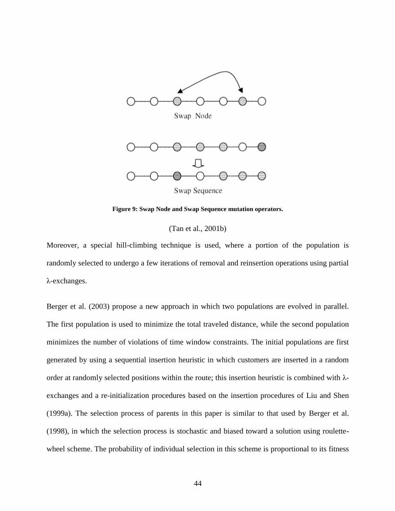
44
Figure 9: Swap Node and Swap Sequence mutation operators.
(Tan et al., 2001b)
Moreover, a special hill-climbing technique is used, where a portion of the population is
randomly selected to undergo a few iterations of removal and reinsertion operations using partial
λ-exchanges.
Berger et al. (2003) propose a new approach in which two populations are evolved in parallel.
The first population is used to minimize the total traveled distance, while the second population
minimizes the number of violations of time window constraints. The initial populations are first
generated by using a sequential insertion heuristic in which customers are inserted in a random
order at randomly selected positions within the route; this insertion heuristic is combined with λ-
exchanges and a re-initialization procedures based on the insertion procedures of Liu and Shen
(1999a). The selection process of parents in this paper is similar to that used by Berger et al.
(1998), in which the selection process is stochastic and biased toward a solution using roulette-
wheel scheme. The probability of individual selection in this scheme is proportional to its fitness
45
value. The authors use two recombining operators, the first operator is the same as that used by
Berger et al. (1998), while the second operator is an extension of the first operator, as it removes
illegal routed customers and uses the insertion procedure that is proposed by Liu and Shen
(1999a) instead of Solomon (1987) insertion heuristic. Five mutation operators are used
randomly by the authors; one of these operators is based on large neighborhood search, while the
other mutation operators involve λ-exchanges (inter-route improvement), elimination of the
shortest route using the procedure of Liu and Shen (1999a), and within route reordering using the
heuristic proposed by Solomon (1987).
Alvarengaa et al. (2007) propose an algorithms that combines GA with set partitioning
formulation for solving VRPTW. The authors propose a GA to generate routes for the main set
partitioning formulation. The chromosome is defined as a string of integers that represents a
route to be serviced by only one vehicle. A modified Push Forward Insertion Heuristic (PFIH)
called stochastic PFIH is used to generate the initial population for the GA. A k-way tournament
selection method is used for nominating the parents for a crossover. The individuals in the
proposed algorithm are evaluated by using a fitness function that depends on the inverse of the
total traveled distance. A new crossover strategy is used to produce new generations, in which
the algorithm makes a random route choice from each parent individual in turns, and after all
feasible routes have been inserted in the offspring, the insertion of remaining customers is tested
in existing routes. If some customers continue to be un-routed, stochastic PFIH is applied to
insert un-routed customers. In order to maintain the quality of solution achieved so far, the
elitism strategy is adopted, in which best individuals from the current solution are added to the
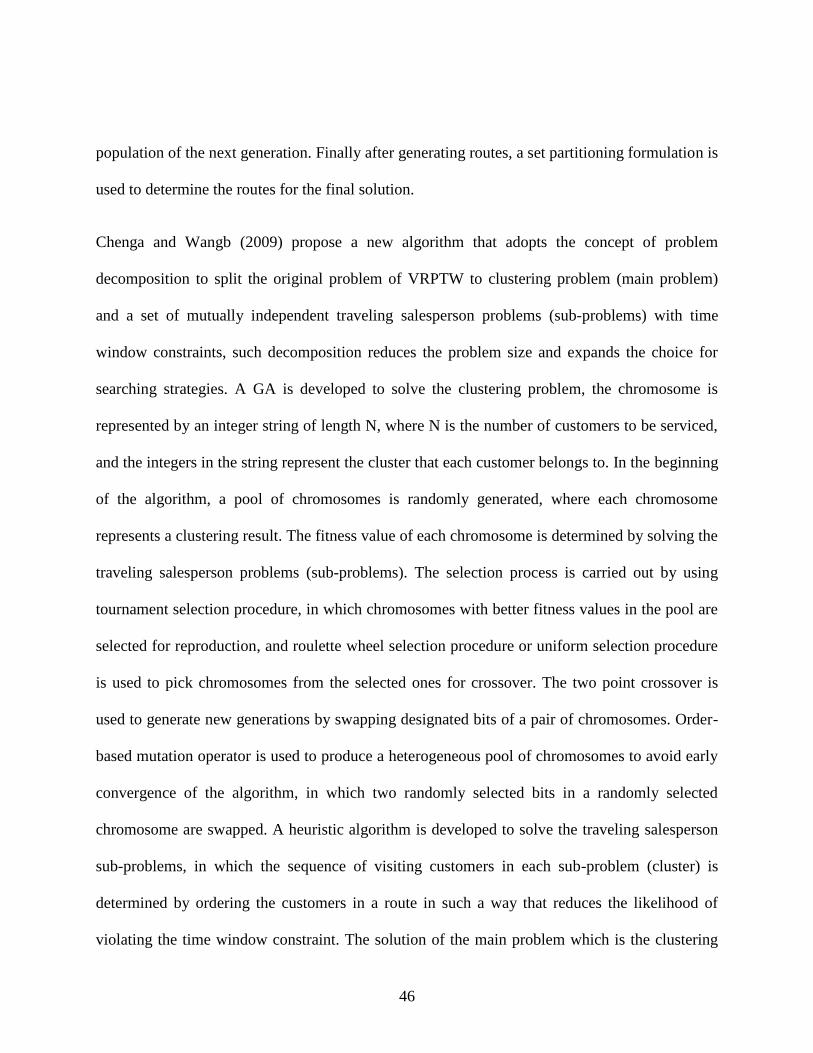
46
population of the next generation. Finally after generating routes, a set partitioning formulation is
used to determine the routes for the final solution.
Chenga and Wangb (2009) propose a new algorithm that adopts the concept of problem
decomposition to split the original problem of VRPTW to clustering problem (main problem)
and a set of mutually independent traveling salesperson problems (sub-problems) with time
window constraints, such decomposition reduces the problem size and expands the choice for
searching strategies. A GA is developed to solve the clustering problem, the chromosome is
represented by an integer string of length N, where N is the number of customers to be serviced,
and the integers in the string represent the cluster that each customer belongs to. In the beginning
of the algorithm, a pool of chromosomes is randomly generated, where each chromosome
represents a clustering result. The fitness value of each chromosome is determined by solving the
traveling salesperson problems (sub-problems). The selection process is carried out by using
tournament selection procedure, in which chromosomes with better fitness values in the pool are
selected for reproduction, and roulette wheel selection procedure or uniform selection procedure
is used to pick chromosomes from the selected ones for crossover. The two point crossover is
used to generate new generations by swapping designated bits of a pair of chromosomes. Order-
based mutation operator is used to produce a heterogeneous pool of chromosomes to avoid early
convergence of the algorithm, in which two randomly selected bits in a randomly selected
chromosome are swapped. A heuristic algorithm is developed to solve the traveling salesperson
sub-problems, in which the sequence of visiting customers in each sub-problem (cluster) is
determined by ordering the customers in a route in such a way that reduces the likelihood of
violating the time window constraint. The solution of the main problem which is the clustering

47
process is obtained through iterative interactions between the main problem and the set of sub-
problems.
Nazif and Lee (2010) propose a GA for VRPTW that the authors call the Optimized Crossover
Genetic Algorithm (OCGA). The representation of a solution is in the form of an integer string
of length N, where N is the number of customers to be serviced, and each gene (integer) in the
string represents a number that is assigned originally to a certain customer, while the sequence of
the genes in the string is the order of visiting these customers. The initial population is generated
randomly by using a random number generator, while the selection process is based on a
probabilistic tournament scheme to select parents from the population. The authors propose an
optimized crossover scheme that uses undirected bipartite graph to determine all perfect
matching that finally produces two new children which are called O-child and E-child. The
authors use two different mutation operators called inversion and swap sequence operators, the
inversion operator reverses the sequence of visiting customers between two randomly selected
points, while the swap sequence operator exchanges the positions of the two sub-strings of
customers that are randomly selected.
2.4.2.2 Ant Colony Optimization
Ant Colony Optimization (ACO) is a meta-heuristic proposed by Dorigo et al. (1996); Dorigo &
Caro (1999); Dorigo & Stützle (2003). ACO is inspired by the foraging behavior of real ants; the
behavior that enables ants to find the shortest paths between food sources and their nest.

48
In the real ant colony, as ants walk from food sources to the nest and vice versa, they deposit a
substance called pheromone on the ground. Ant selection of direction to follow between food
sources and nest is determined according to the strength of pheromone concentration; such basic
behavior leads to the emergence of the shortest paths.
ACO algorithms are based on a probabilistic model (pheromone model) that is used to model the
chemical pheromone trails. The artificial ants incrementally construct feasible solutions
sequentially. To achieve this, the ants perform randomized walks on a completely connected
graph whose vertices (nodes) are the solution components C and the set L are the
connections. Each ant chooses each successive node with a probability that is a function of the
node distance and the amount of pheromone trail (trail intensity) present on the connecting edge.
The move from certain node to the next is one iteration. A complete tour is constructed by
performing n iterations that visit the n available customers. In order to ensure tour validity, the
transition to the already visited nodes is prohibited until a tour is completed (controlled by a
Tabu list). When a tour is completed, each ant lays a substance called a trail on each visited edge.
This process is iterated until the tour reaches the maximum number of cycles or all ants make the
same tour which is called stagnation behavior.
Gambardella et al. (1999) propose a Multi-objective Ant Colony System for solving VRPTW
(MACS-VRPTW). The objective of this ant colony system is to minimize the number of used
vehicles and the total travel distance. The proposed algorithm uses a hierarchy of two artificial
ant colonies; each one dealing with one of the objectives. The first colony is named ACS-VEI
and deals with the number of tours (vehicles) minimization while ACS-Time minimizes the
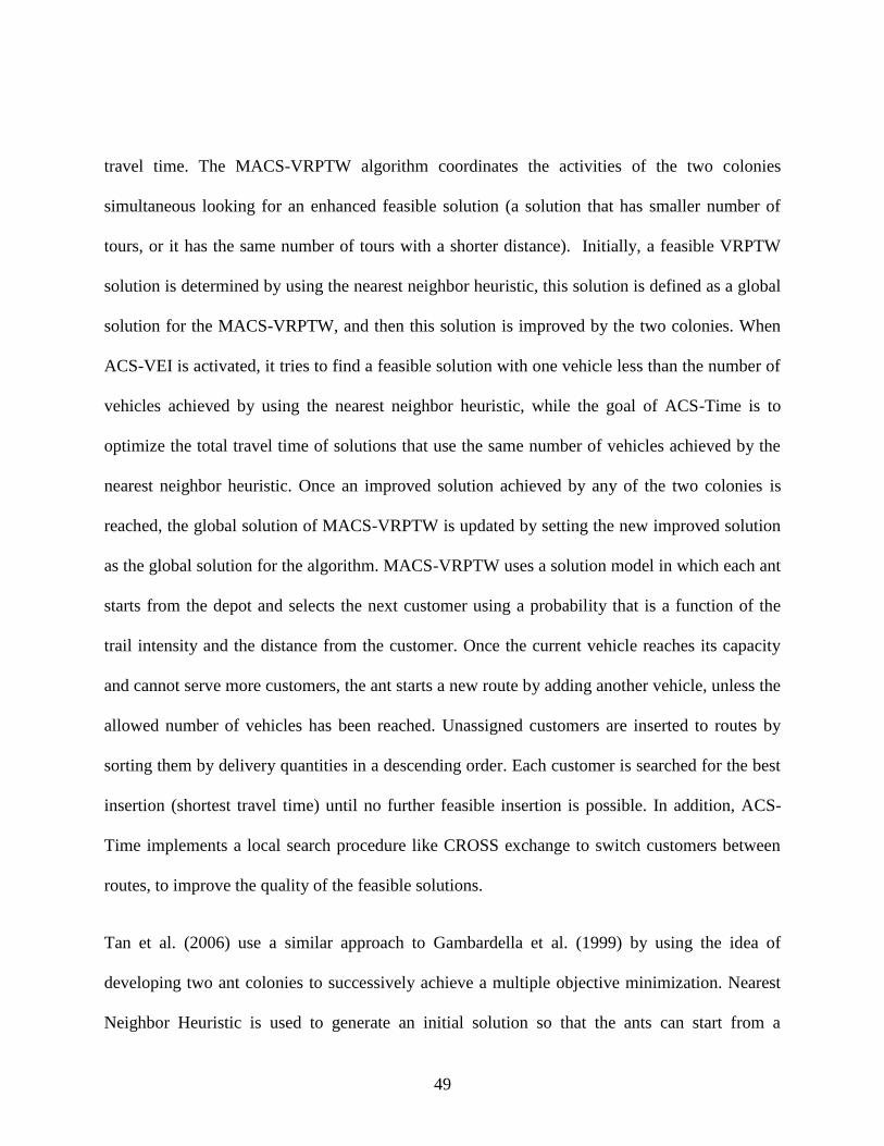
49
travel time. The MACS-VRPTW algorithm coordinates the activities of the two colonies
simultaneous looking for an enhanced feasible solution (a solution that has smaller number of
tours, or it has the same number of tours with a shorter distance). Initially, a feasible VRPTW
solution is determined by using the nearest neighbor heuristic, this solution is defined as a global
solution for the MACS-VRPTW, and then this solution is improved by the two colonies. When
ACS-VEI is activated, it tries to find a feasible solution with one vehicle less than the number of
vehicles achieved by using the nearest neighbor heuristic, while the goal of ACS-Time is to
optimize the total travel time of solutions that use the same number of vehicles achieved by the
nearest neighbor heuristic. Once an improved solution achieved by any of the two colonies is
reached, the global solution of MACS-VRPTW is updated by setting the new improved solution
as the global solution for the algorithm. MACS-VRPTW uses a solution model in which each ant
starts from the depot and selects the next customer using a probability that is a function of the
trail intensity and the distance from the customer. Once the current vehicle reaches its capacity
and cannot serve more customers, the ant starts a new route by adding another vehicle, unless the
allowed number of vehicles has been reached. Unassigned customers are inserted to routes by
sorting them by delivery quantities in a descending order. Each customer is searched for the best
insertion (shortest travel time) until no further feasible insertion is possible. In addition, ACS-
Time implements a local search procedure like CROSS exchange to switch customers between
routes, to improve the quality of the feasible solutions.
Tan et al. (2006) use a similar approach to Gambardella et al. (1999) by using the idea of
developing two ant colonies to successively achieve a multiple objective minimization. Nearest
Neighbor Heuristic is used to generate an initial solution so that the ants can start from a
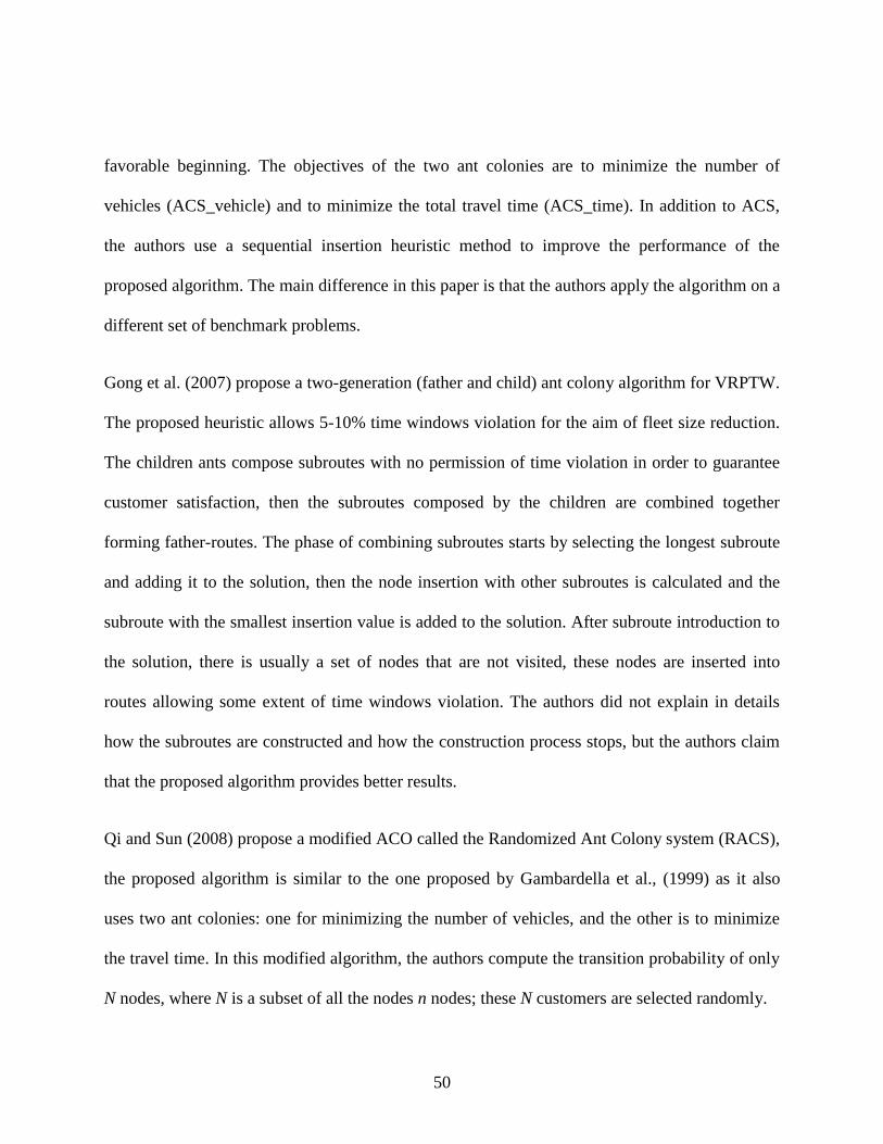
50
favorable beginning. The objectives of the two ant colonies are to minimize the number of
vehicles (ACS_vehicle) and to minimize the total travel time (ACS_time). In addition to ACS,
the authors use a sequential insertion heuristic method to improve the performance of the
proposed algorithm. The main difference in this paper is that the authors apply the algorithm on a
different set of benchmark problems.
Gong et al. (2007) propose a two-generation (father and child) ant colony algorithm for VRPTW.
The proposed heuristic allows 5-10% time windows violation for the aim of fleet size reduction.
The children ants compose subroutes with no permission of time violation in order to guarantee
customer satisfaction, then the subroutes composed by the children are combined together
forming father-routes. The phase of combining subroutes starts by selecting the longest subroute
and adding it to the solution, then the node insertion with other subroutes is calculated and the
subroute with the smallest insertion value is added to the solution. After subroute introduction to
the solution, there is usually a set of nodes that are not visited, these nodes are inserted into
routes allowing some extent of time windows violation. The authors did not explain in details
how the subroutes are constructed and how the construction process stops, but the authors claim
that the proposed algorithm provides better results.
Qi and Sun (2008) propose a modified ACO called the Randomized Ant Colony system (RACS),
the proposed algorithm is similar to the one proposed by Gambardella et al., (1999) as it also
uses two ant colonies: one for minimizing the number of vehicles, and the other is to minimize
the travel time. In this modified algorithm, the authors compute the transition probability of only
N nodes, where N is a subset of all the nodes n nodes; these N customers are selected randomly.

51
2.5 Summary and Research Gap
Much of the research on VRPTW focuses on finding an optimal or near-optimal solution to the
problem through the use of exact algorithms, heuristics or metaheuristics.
A summary of the different approaches proposed in literature to solve the problem of VRPTW
are presented in Table 1.
No previous work addresses the problem of scheduling the dispatching of vehicles from a depot
with limited number of docks while satisfying customer time windows. Often in real-life
settings, the number of vehicles to be dispatched simultaneously from a depot is larger than the
number of docks. This creates an additional constraint in the VRPTW forcing the vehicles to be
dispatched at different times, which has a direct impact on satisfying the customers’ time
windows. Hence, a VRPTW schedule that is created while ignoring the limited number of docks
may not be feasible. This research investigates the VRPTW with limited number of docks at the
depot. Chapter 3 presents the proposed methodology to solve this problem.
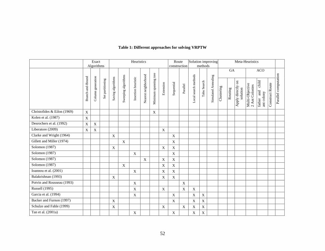
52
Table 1: Different approaches for solving VRPTW
Exact
Algorithms
Heuristics Route
construction
Solution improving
methods
Meta-Heuristics
Bra
nch
-and
-Bou
nd
Colu
mn
gen
erat
ion
Set
par
titi
onin
g
Sav
ing
alg
ori
thm
s
Sw
eepin
g a
lgo
rith
ms
Inse
rtio
n h
euri
stic
Nea
rest
nei
gh
bo
rhoo
d
Min
imu
m s
pan
nin
g t
ree
Ex
tensi
on
Seq
uen
tial
Par
alle
l
Lo
cal
sear
ch m
ethod
s
Tab
u S
earc
h
Sim
ula
ted
Annea
lin
g
GA ACO
Par
alle
l co
mp
uta
tio
n
Clu
ster
ing
Ro
uti
ng
Ap
ply
dir
ectl
y o
n
solu
tio
n
Mu
lti-
Ob
ject
ive
2 A
nt
Co
lon
ies
fath
er
and
ch
ild
ant
colo
ny
Co
nst
ruct
Rou
te
Christofides & Eilon (1969) X X
Kolen et al. (1987) X
Desrochers et al. (1992) X X
Liberatore (2009) X X X
Clarke and Wright (1964) X X
Gillett and Miller (1974) X X
Solomon (1987) X X X
Solomon (1987) X X
Solomon (1987) X X X
Solomon (1987) X X X
Ioannou et al. (2001) X X X
Balakrishnan (1993) X X X
Potvin and Rousseau (1993) X X
Russell (1995) X X X X
Garcia et al. (1994) X X X X
Backer and Furnon (1997) X X X X
Schulze and Fahle (1999) X X X X X
Tan et al. (2001a) X X X X
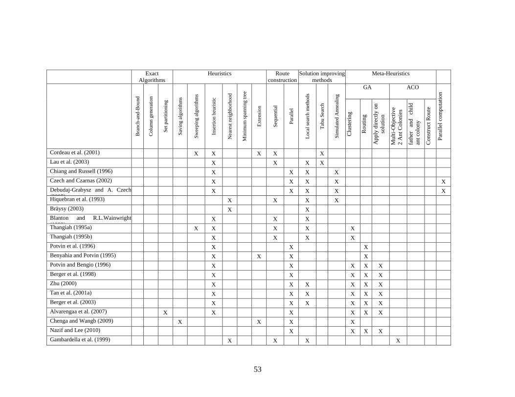
53
Exact
Algorithms
Heuristics Route
construction
Solution improving
methods
Meta-Heuristics
Bra
nch
-and
-Bou
nd
Colu
mn
gen
erat
ion
Set
par
titi
onin
g
Sav
ing
alg
ori
thm
s
Sw
eepin
g a
lgo
rith
ms
Inse
rtio
n h
euri
stic
Nea
rest
nei
gh
bo
rhoo
d
Min
imu
m s
pan
nin
g t
ree
Ex
tensi
on
Seq
uen
tial
Par
alle
l
Lo
cal
sear
ch m
ethod
s
Tab
u S
earc
h
Sim
ula
ted
Annea
lin
g
GA ACO
Par
alle
l co
mp
uta
tio
n
Clu
ster
ing
Ro
uti
ng
Ap
ply
dir
ectl
y o
n
solu
tio
n
Mu
lti-
Ob
ject
ive
2 A
nt
Co
lon
ies
fath
er
and
ch
ild
ant
colo
ny
Co
nst
ruct
Rou
te
Cordeau et al. (2001) X X X X X
Lau et al. (2003) X X X X
Chiang and Russell (1996) X X X X
Czech and Czarnas (2002) X X X X X
Debudaj-Grabysz and A. Czech
(2005) X X X X X
Hiquebran et al. (1993) X X X X
Bräysy (2003) X X
Blanton and R.L.Wainwright
(1993) X X X
Thangiah (1995a) X X X X X
Thangiah (1995b) X X X X
Potvin et al. (1996) X X X
Benyahia and Potvin (1995) X X X X
Potvin and Bengio (1996) X X X X X
Berger et al. (1998) X X X X X
Zhu (2000) X X X X X X
Tan et al. (2001a) X X X X X X
Berger et al. (2003) X X X X X X
Alvarengaa et al. (2007) X X X X X X
Chenga and Wangb (2009) X X X X
Nazif and Lee (2010) X X X X
Gambardella et al. (1999) X X X X
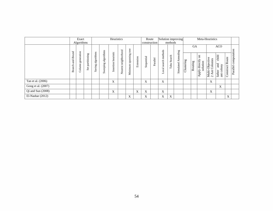
54
Exact
Algorithms
Heuristics Route
construction
Solution improving
methods
Meta-Heuristics
Bra
nch
-and
-Bou
nd
Colu
mn
gen
erat
ion
Set
par
titi
onin
g
Sav
ing
alg
ori
thm
s
Sw
eepin
g a
lgo
rith
ms
Inse
rtio
n h
euri
stic
Nea
rest
nei
gh
bo
rhoo
d
Min
imu
m s
pan
nin
g t
ree
Ex
tensi
on
Seq
uen
tial
Par
alle
l
Lo
cal
sear
ch m
ethod
s
Tab
u S
earc
h
Sim
ula
ted
Annea
lin
g
GA ACO
Par
alle
l co
mp
uta
tio
n
Clu
ster
ing
Ro
uti
ng
Ap
ply
dir
ectl
y o
n
solu
tio
n
Mu
lti-
Ob
ject
ive
2 A
nt
Co
lon
ies
fath
er
and
ch
ild
ant
colo
ny
Co
nst
ruct
Rou
te
Tan et al. (2006) X X X X
Gong et al. (2007) X
Qi and Sun (2008) X X X X X
El-Nashar (2012) X X X X X
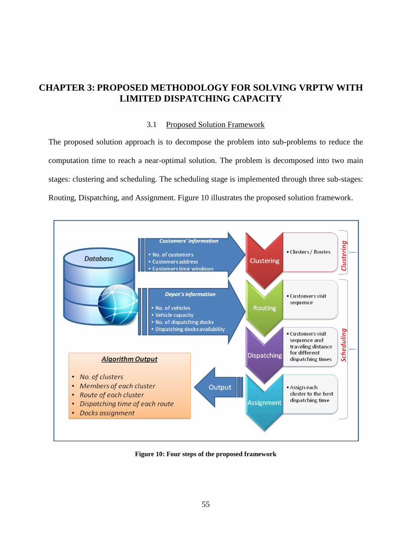
55
CHAPTER 3: PROPOSED METHODOLOGY FOR SOLVING VRPTW WITH
LIMITED DISPATCHING CAPACITY
3.1 Proposed Solution Framework
The proposed solution approach is to decompose the problem into sub-problems to reduce the
computation time to reach a near-optimal solution. The problem is decomposed into two main
stages: clustering and scheduling. The scheduling stage is implemented through three sub-stages:
Routing, Dispatching, and Assignment. Figure 10 illustrates the proposed solution framework.
Figure 10: Four steps of the proposed framework
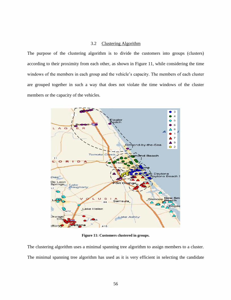
56
3.2 Clustering Algorithm
The purpose of the clustering algorithm is to divide the customers into groups (clusters)
according to their proximity from each other, as shown in Figure 11, while considering the time
windows of the members in each group and the vehicle’s capacity. The members of each cluster
are grouped together in such a way that does not violate the time windows of the cluster
members or the capacity of the vehicles.
Figure 11: Customers clustered in groups.
The clustering algorithm uses a minimal spanning tree algorithm to assign members to a cluster.
The minimal spanning tree algorithm has used as it is very efficient in selecting the candidate
57
customer to be added to cluster, this algorithm has been used by Christofides et al., (1981) for
constructing routes in the case of Vehicle Routing Problem.
3.2.1 The Mechanics of Clustering Algorithm
The mechanism and steps of the clustering algorithm are illustrated in details in Figure 12.
Initially, each cluster has one customer, and therefore, the number of clusters is equal to the
number of customers.
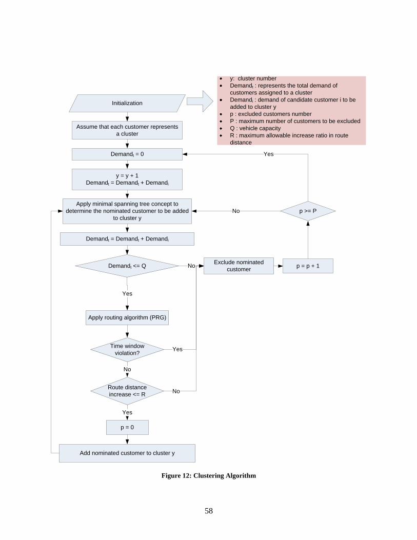
58
Assume that each customer represents
a cluster
Apply minimal spanning tree concept to
determine the nominated customer to be added
to cluster y
Demandt = 0
y = y + 1
Demandt = Demandt + Demandi
Demandt = Demandt + Demandi
Demandt <= Q
No
Exclude nominated
customer No
Apply routing algorithm (PRG)
Yes
Time window
violation?Yes
Add nominated customer to cluster y
No
p = p + 1
p >= P
Route distance
increase <= RNo
Yes
p = 0
Yes
y: cluster number
Demandt : represents the total demand of
customers assigned to a cluster
Demandi : demand of candidate customer i to be
added to cluster y
p : excluded customers number
P : maximum number of customers to be excluded
Q : vehicle capacity
R : maximum allowable increase ratio in route
distance
Initialization
Figure 12: Clustering Algorithm
59
The algorithm starts with the first customer (cluster), and the minimal spanning tree algorithm is
used to determine the nearest customer (candidate) i to the current cluster y. After determining
the nearest customer i, the Probabilistic Route Generation (PRG) algorithm that will be discussed
in Section 3.3 is executed to determine if adding the candidate customer i to the cluster y will
violate the time window of any of the current cluster members. Further, the clustering algorithm
checks if adding the candidate customer i to the cluster y will violate the vehicle capacity Q.
The candidate customer will be added to the cluster if none of the following criteria is violated:
Vehicle capacity
Cluster customers’ time windows
The percentage increase in performance criterion (time, distance or cost) as a result of
adding the candidate customer is less than or equal to a predetermined ratio “ ”; the
method for determining is illustrated in the Section 3.2.1.1
After adding the candidate customer i to the cluster y, the clustering algorithm searches again for
the nearest customer to the current cluster members, and the same previous procedures will be
implemented to add the candidate customer to the cluster.
The clustering algorithm terminates when a specific number of consecutive candidate customers
P could not be added to the cluster due to vehicle capacity violation, time window violation, or
when the percentage increase in route length (time, distance or cost) is higher than the acceptable
ratio .
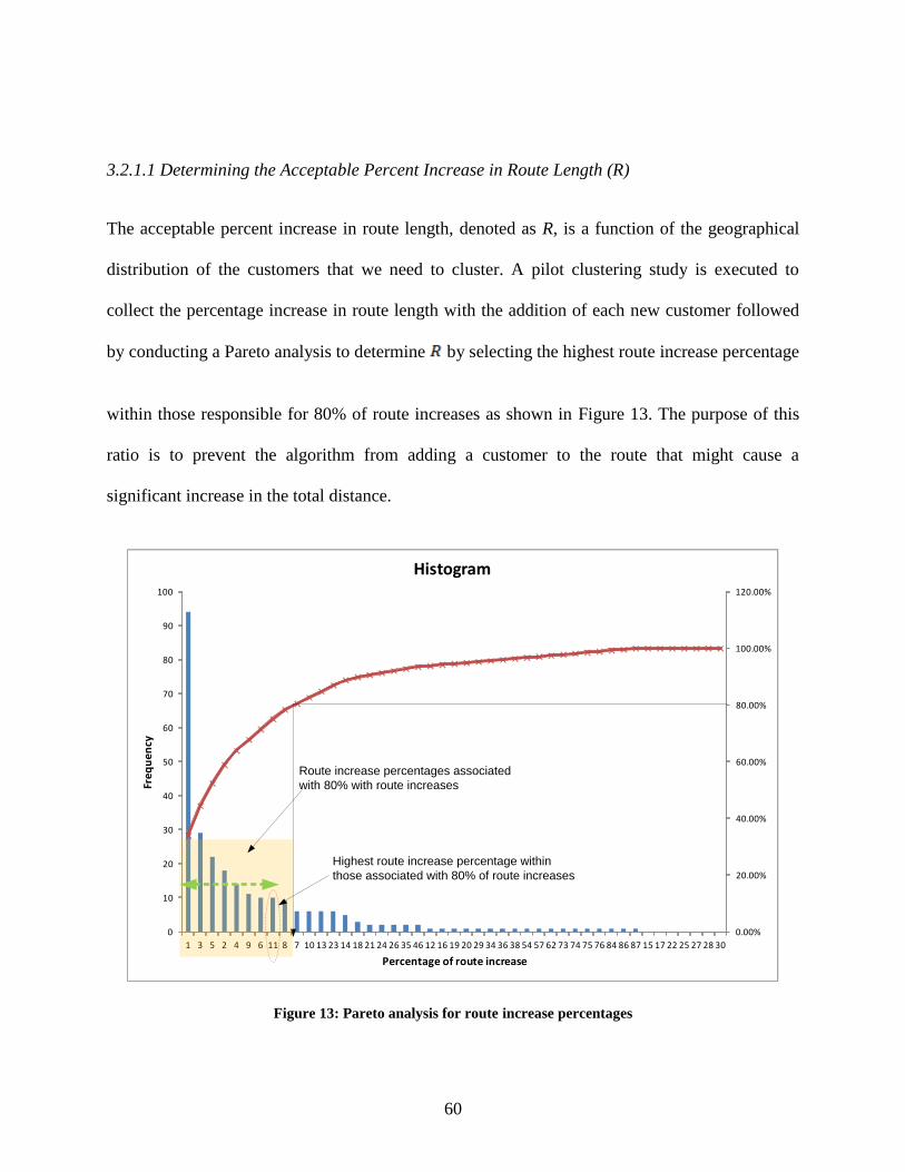
60
3.2.1.1 Determining the Acceptable Percent Increase in Route Length (R)
The acceptable percent increase in route length, denoted as R, is a function of the geographical
distribution of the customers that we need to cluster. A pilot clustering study is executed to
collect the percentage increase in route length with the addition of each new customer followed
by conducting a Pareto analysis to determine by selecting the highest route increase percentage
within those responsible for 80% of route increases as shown in Figure 13. The purpose of this
ratio is to prevent the algorithm from adding a customer to the route that might cause a
significant increase in the total distance.
0.00%
20.00%
40.00%
60.00%
80.00%
100.00%
120.00%
0
10
20
30
40
50
60
70
80
90
100
1 3 5 2 4 9 6 11 8 7 10 13 23 14 18 21 24 26 35 46 12 16 19 20 29 34 36 38 54 57 62 73 74 75 76 84 86 87 15 17 22 25 27 28 30
Fre
qu
en
cy
Percentage of route increase
Histogram
Route increase percentages associated
with 80% with route increases
Highest route increase percentage within
those associated with 80% of route increases
Figure 13: Pareto analysis for route increase percentages
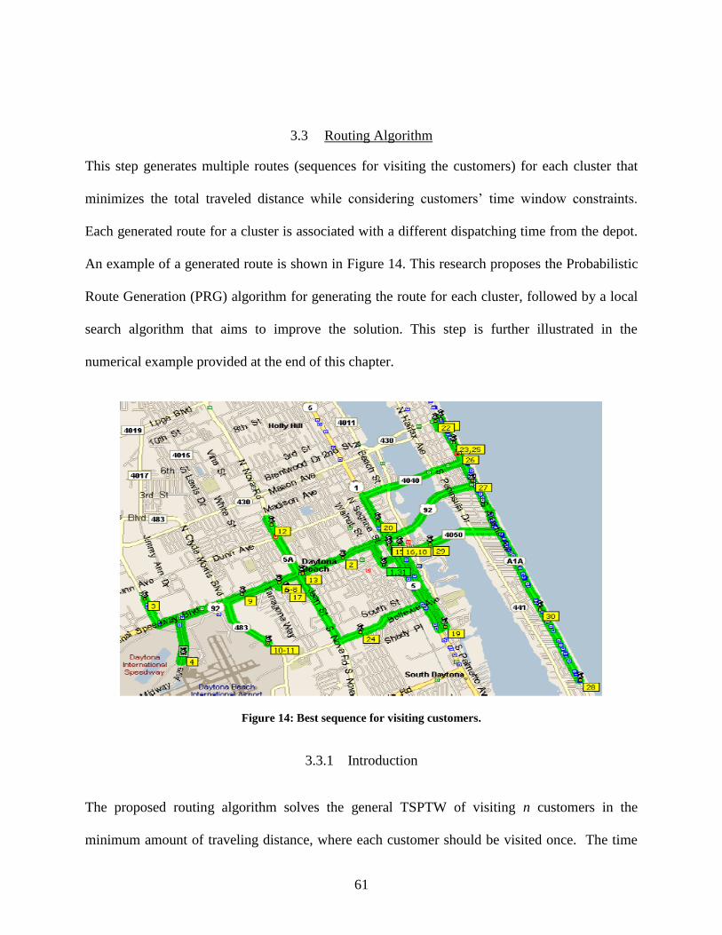
61
3.3 Routing Algorithm
This step generates multiple routes (sequences for visiting the customers) for each cluster that
minimizes the total traveled distance while considering customers’ time window constraints.
Each generated route for a cluster is associated with a different dispatching time from the depot.
An example of a generated route is shown in Figure 14. This research proposes the Probabilistic
Route Generation (PRG) algorithm for generating the route for each cluster, followed by a local
search algorithm that aims to improve the solution. This step is further illustrated in the
numerical example provided at the end of this chapter.
Figure 14: Best sequence for visiting customers.
3.3.1 Introduction
The proposed routing algorithm solves the general TSPTW of visiting n customers in the
minimum amount of traveling distance, where each customer should be visited once. The time
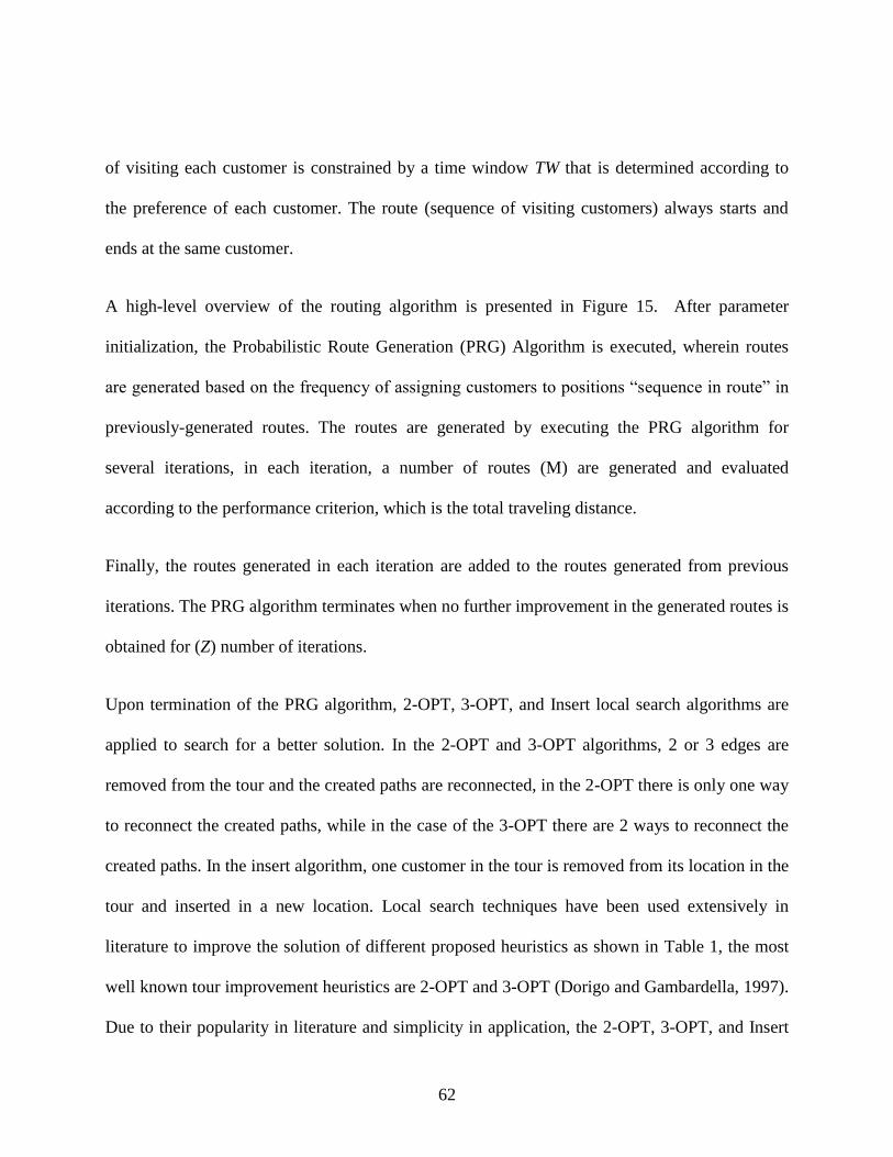
62
of visiting each customer is constrained by a time window TW that is determined according to
the preference of each customer. The route (sequence of visiting customers) always starts and
ends at the same customer.
A high-level overview of the routing algorithm is presented in Figure 15. After parameter
initialization, the Probabilistic Route Generation (PRG) Algorithm is executed, wherein routes
are generated based on the frequency of assigning customers to positions “sequence in route” in
previously-generated routes. The routes are generated by executing the PRG algorithm for
several iterations, in each iteration, a number of routes (M) are generated and evaluated
according to the performance criterion, which is the total traveling distance.
Finally, the routes generated in each iteration are added to the routes generated from previous
iterations. The PRG algorithm terminates when no further improvement in the generated routes is
obtained for (Z) number of iterations.
Upon termination of the PRG algorithm, 2-OPT, 3-OPT, and Insert local search algorithms are
applied to search for a better solution. In the 2-OPT and 3-OPT algorithms, 2 or 3 edges are
removed from the tour and the created paths are reconnected, in the 2-OPT there is only one way
to reconnect the created paths, while in the case of the 3-OPT there are 2 ways to reconnect the
created paths. In the insert algorithm, one customer in the tour is removed from its location in the
tour and inserted in a new location. Local search techniques have been used extensively in
literature to improve the solution of different proposed heuristics as shown in Table 1, the most
well known tour improvement heuristics are 2-OPT and 3-OPT (Dorigo and Gambardella, 1997).
Due to their popularity in literature and simplicity in application, the 2-OPT, 3-OPT, and Insert
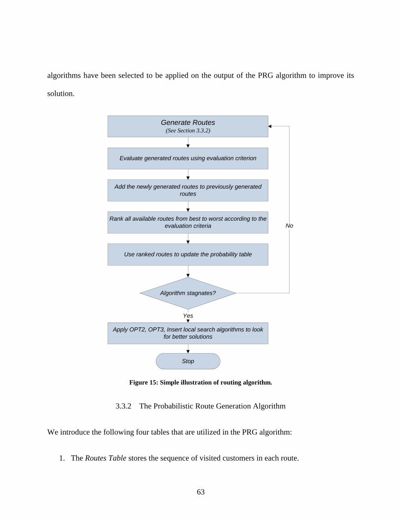
63
algorithms have been selected to be applied on the output of the PRG algorithm to improve its
solution.
Generate Routes(See Section 3.3.2)
Evaluate generated routes using evaluation criterion
Add the newly generated routes to previously generated
routes
Rank all available routes from best to worst according to the
evaluation criteria
Use ranked routes to update the probability table
Algorithm stagnates?
Stop
Yes
No
Apply OPT2, OPT3, Insert local search algorithms to look
for better solutions
Figure 15: Simple illustration of routing algorithm.
3.3.2 The Probabilistic Route Generation Algorithm
We introduce the following four tables that are utilized in the PRG algorithm:
1. The Routes Table stores the sequence of visited customers in each route.

64
2. The Frequency Table stores the number of times each customer appears in each route
position.
3. The Probability Table stores the probability of having each customer in each position
(referred to as customer-position combination) of the route.
4. The Cumulative Probability Table stores the cumulative probability associated with each
customer-position combination in a route.
The role of each table in the routing algorithm is discussed next.
3.3.2.1 The Routes Table
An example of a generated Routes Table is shown in Figure 16. The rows in iteration represent
the routes generated by the algorithm up to and including iteration z. The number of rows in this
table represents the number of generated routes to this point across all iterations, denoted by (r2) ,
where rz = M * z, and therefore, at initialization, z = 0, and rz = 0, and the Routes Table is empty.
The table has (Ny + 1) columns, where Ny represent the number of customers in cluster y, and
without loss of generality, the first and the last columns have the value “1”, which represents the
starting and ending customer of the route. The rows are always ranked from best to worst value
for the performance criterion.
Generated
route
Corresponding
distance to that
route
The second position
in each route
Figure 16: Generated Routes Table.
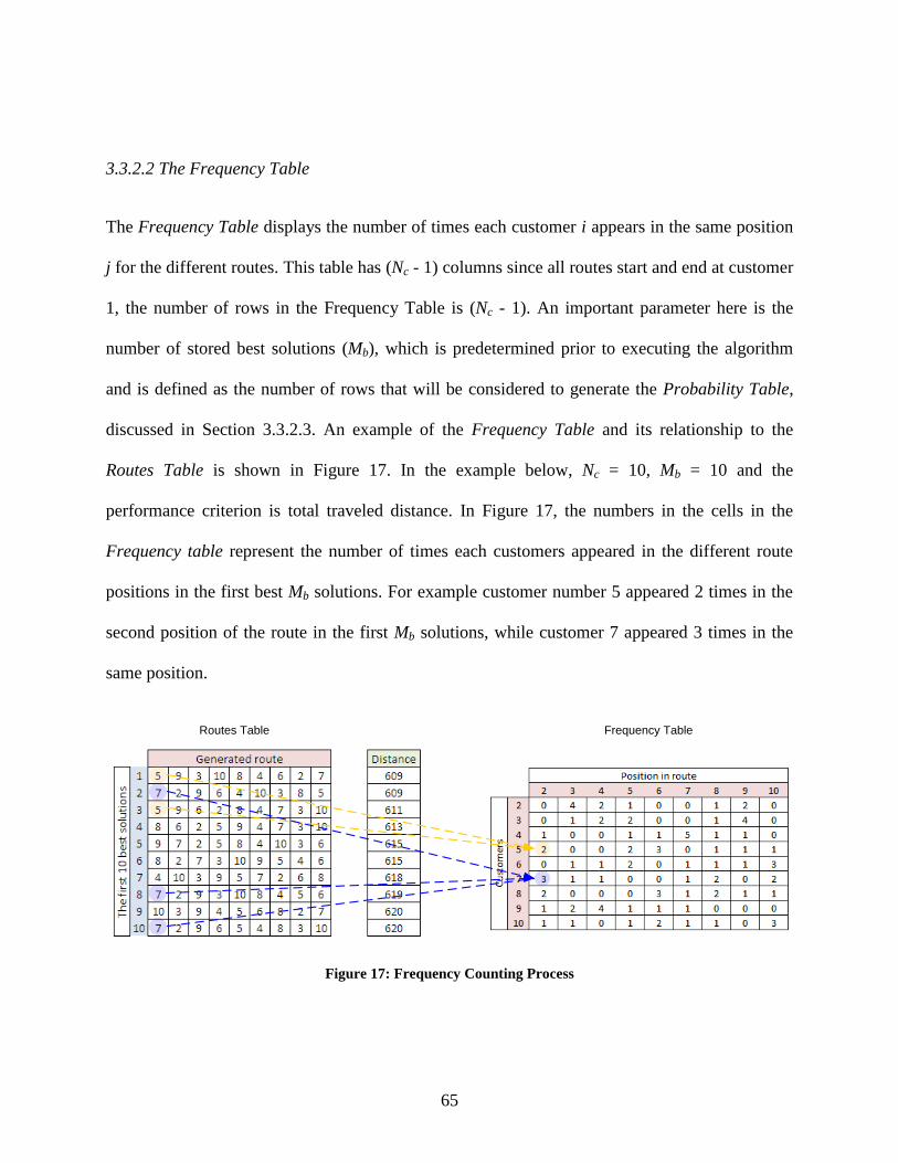
65
3.3.2.2 The Frequency Table
The Frequency Table displays the number of times each customer i appears in the same position
j for the different routes. This table has (Nc - 1) columns since all routes start and end at customer
1, the number of rows in the Frequency Table is (Nc - 1). An important parameter here is the
number of stored best solutions (Mb), which is predetermined prior to executing the algorithm
and is defined as the number of rows that will be considered to generate the Probability Table,
discussed in Section 3.3.2.3. An example of the Frequency Table and its relationship to the
Routes Table is shown in Figure 17. In the example below, Nc = 10, Mb = 10 and the
performance criterion is total traveled distance. In Figure 17, the numbers in the cells in the
Frequency table represent the number of times each customers appeared in the different route
positions in the first best Mb solutions. For example customer number 5 appeared 2 times in the
second position of the route in the first Mb solutions, while customer 7 appeared 3 times in the
same position.
Routes Table Frequency Table
Figure 17: Frequency Counting Process
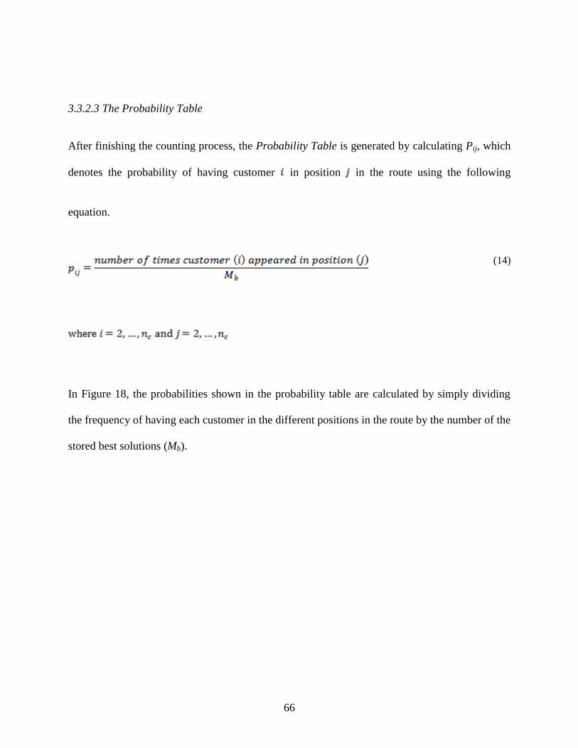
66
3.3.2.3 The Probability Table
After finishing the counting process, the Probability Table is generated by calculating Pij, which
denotes the probability of having customer in position in the route using the following
equation.
(14)
In Figure 18, the probabilities shown in the probability table are calculated by simply dividing
the frequency of having each customer in the different positions in the route by the number of the
stored best solutions (Mb).
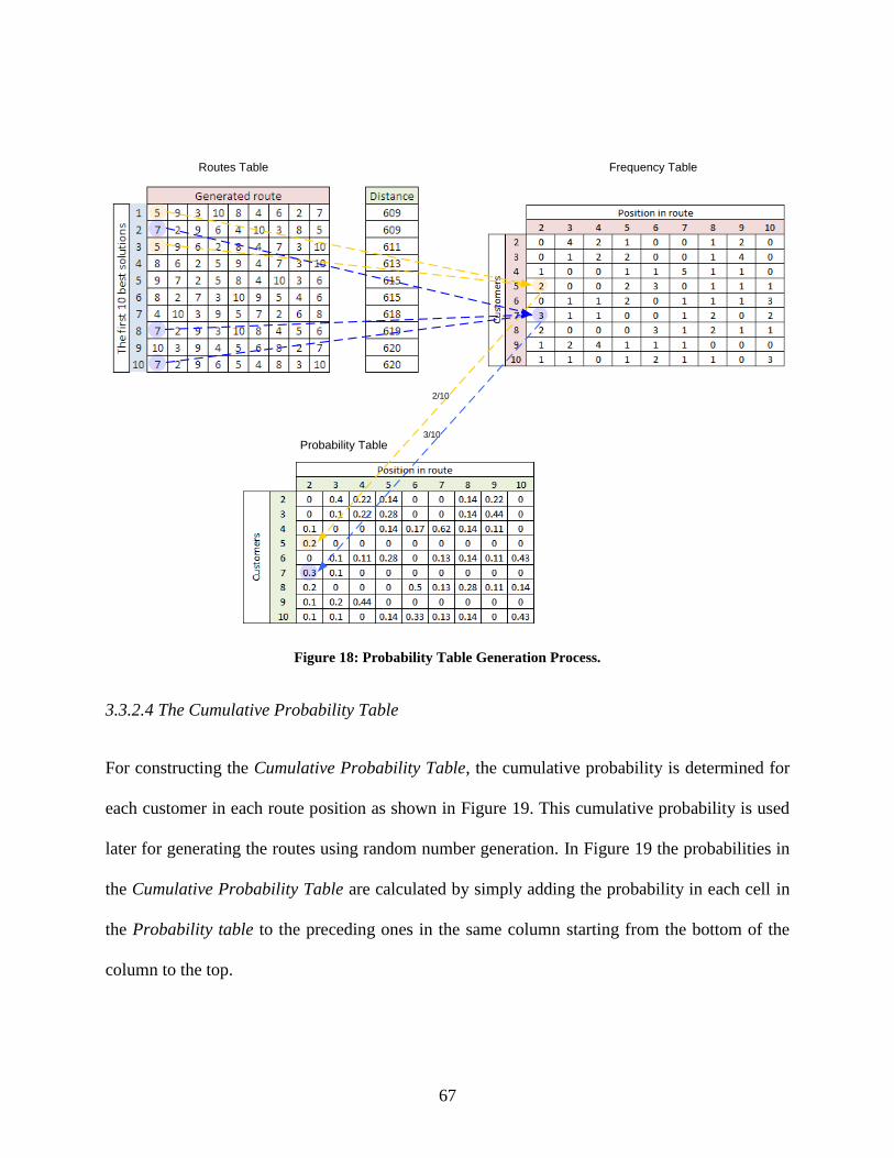
67
Routes Table Frequency Table
2/10
3/10
Probability Table
Figure 18: Probability Table Generation Process.
3.3.2.4 The Cumulative Probability Table
For constructing the Cumulative Probability Table, the cumulative probability is determined for
each customer in each route position as shown in Figure 19. This cumulative probability is used
later for generating the routes using random number generation. In Figure 19 the probabilities in
the Cumulative Probability Table are calculated by simply adding the probability in each cell in
the Probability table to the preceding ones in the same column starting from the bottom of the
column to the top.

68
Routes Table Frequency Table
2/10
3/10
Probability TableCumulative Probability Table
Figure 19: Cumulative Probability Table
The main purpose of the four tables is to update the cumulative probabilities after each iteration.
Initially, when algorithm starts generating the first iteration’s route, the customers have equal
probabilities of appearing in each position in the route.
3.3.3 PRG Algorithm Mechanics
The overall routing algorithm is summarized in the flow chart illustrated in Figure 20.
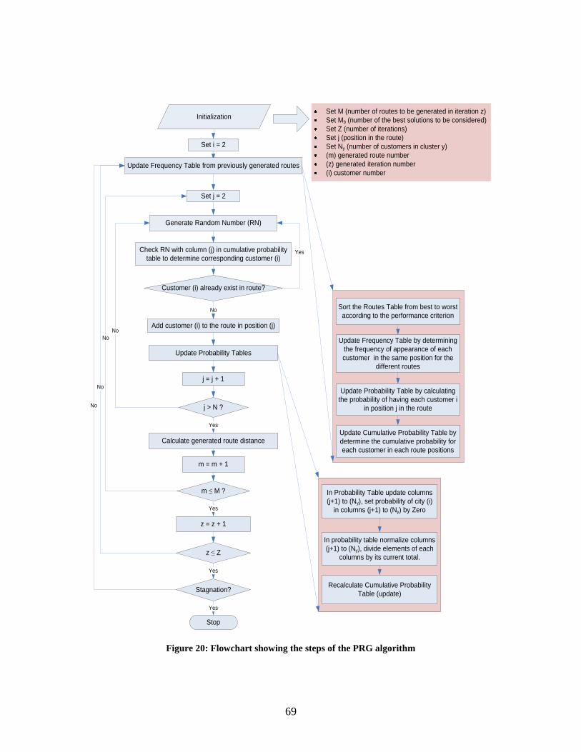
69
Set j = 2
Generate Random Number (RN)
Check RN with column (j) in cumulative probability
table to determine corresponding customer (i)
Customer (i) already exist in route?
Yes
Update Probability Tables
No
j = j + 1
j > N ?
No
Stop
Yes
Add customer (i) to the route in position (j)
m = m + 1
m ≤ M ?
No
Set i = 2
z = z + 1
Yes
z ≤ Z
No
Stagnation?
No
Yes
Yes
Calculate generated route distance
In Probability Table update columns
(j+1) to (Ny), set probability of city (i)
in columns (j+1) to (Ny) by Zero
In probability table normalize columns
(j+1) to (Ny), divide elements of each
columns by its current total.
Recalculate Cumulative Probability
Table (update)
Initialization
Update Frequency Table from previously generated routes
Sort the Routes Table from best to worst
according to the performance criterion
Update Frequency Table by determining
the frequency of appearance of each
customer in the same position for the
different routes
Update Probability Table by calculating
the probability of having each customer i
in position j in the route
Update Cumulative Probability Table by
determine the cumulative probability for
each customer in each route positions
Set M (number of routes to be generated in iteration z)
Set Mb (number of the best solutions to be considered)
Set Z (number of iterations)
Set j (position in the route)
Set Ny (number of customers in cluster y)
(m) generated route number
(z) generated iteration number
(i) customer number
Figure 20: Flowchart showing the steps of the PRG algorithm
70
3.3.3.1 Algorithm Initialization
At initialization of the algorithm, the probabilities in the Probability Table are all equal,
indicating that each customer has equal probability of appearing in any position. This assumption
allows the algorithm to generate random routes by allocating any customer to any position
“sequence” in the route without any prior preference.
3.3.3.2 PRG Algorithm Description
Each iteration (z) consists of (M) routes; a predetermined parameter. Each of the (M) routes are
obtained by first generating a random number to determine the customer that should be visited in
each position in the route, we assume, without loss of generality, that customer “1” is the first
customer in the route. To determine the customer in the jth
position, the generated random
number is compared to the jth
column in the Cumulative Probability Table to determine the
customer number i corresponding to that random number.
In order to prevent customers’ replication in a route, we check if customer i is already in the
route. If it does not exist, we add customer i to position j in the route; otherwise, we go back and
generate another random number.
After customer i is added to the route we update the Probability Table by setting the probability
of customer i in columns j + 1 through Ny to zero, and then we normalize these columns by
dividing each element in these columns by the current total of each column to ignore customer i
when generating the rest of the route, and finally we regenerate the Cumulative Probability Table
to be used in the generation of the next route. The previously illustrated steps are repeated until
the route is completed, in other words until all Ny customers have joined the route.

71
The process of constructing the routes is repeated until (M) routes are generated, which are
sorted later from best to worst in terms of the performance criterion, the total traveling distance
of the route, and then used to update the Probability Table. The process of generating routes,
sorting them and updating the Probability Table is continued until the maximum number of
iterations is reached or until the enhancement in the performance criterion stops or stagnates. An
illustrative example for route construction process is shown in Figure 21. In this example let’s
start with the table in upper left corner as the route is completely empty. The first step is to
generate a random number to determine the corresponding customer in the Cumulative
Probability Table to be added to the route, it has been found in this example to be customer 5. As
long as the route is empty, customer 5 is added to the route in its first position after the depot,
and then another random number is generated to determine the customer in the second position.
This process is repeated until all Ny customers are added to the route.
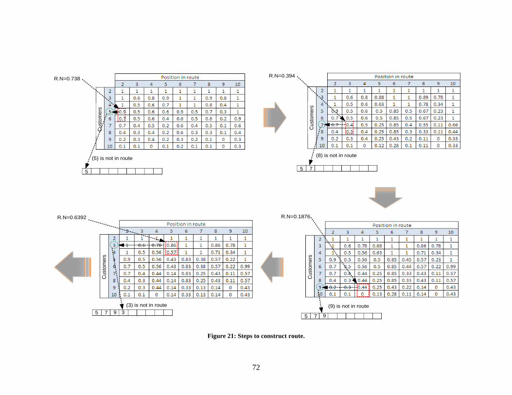
72
R.N=0.738
5
R.N=0.394
5 7
(5) is not in route(8) is not in route
R.N=0.1876
5 7
(9) is not in route
9
R.N=0.6392
(3) is not in route
5 7 9 3
Cu
sto
me
rs
Cu
sto
me
rsC
ust
om
ers
Cu
sto
me
rs
Figure 21: Steps to construct route.
73
3.3.4 Local Search
When the improvement in the solution stagnates, local search algorithms 2-OPT, 3-OPT, and
Insert local are applied on each route of the best H solutions achieved form the PRG algorithm to
achieve better results. The best output of the three algorithms is selected and set as the current
route. The three algorithms are continued to be applied and the best route is selected until no
more improvement in the performance criterion is achieved. This process is summarized in the
flow chart shown in Figure 22.

74
Set h = 1
Apply OPT2 Algorithm on route h
Apply OPT3 Algorithm on route h
Apply Insert Algorithm on route h
Select the best output of the 3
algorithms
Set current solution = solution of route h
Best
output better than current
solution?
Set current route = route h
Set current solution = solution of best
output
Set current route = route of best output
Yes
Set h = h +1
No
h > H?
Stop
Yes
No
InitializationSet (H) number of routes, the local
search applied on
Figure 22: Applying local search algorithms to achieve better solutions
3.3.5 Assigning Dispatching Times
This step assigns a dispatching time from the depot to each cluster (vehicle) in order to minimize
the total traveled distance. The problem is solved as an assignment problem, the assignment
process is illustrated with a numerical example that consists of 241 customers, 50% of which
have time window constraints. The customers are to be served in a one day shift of 12 hours.
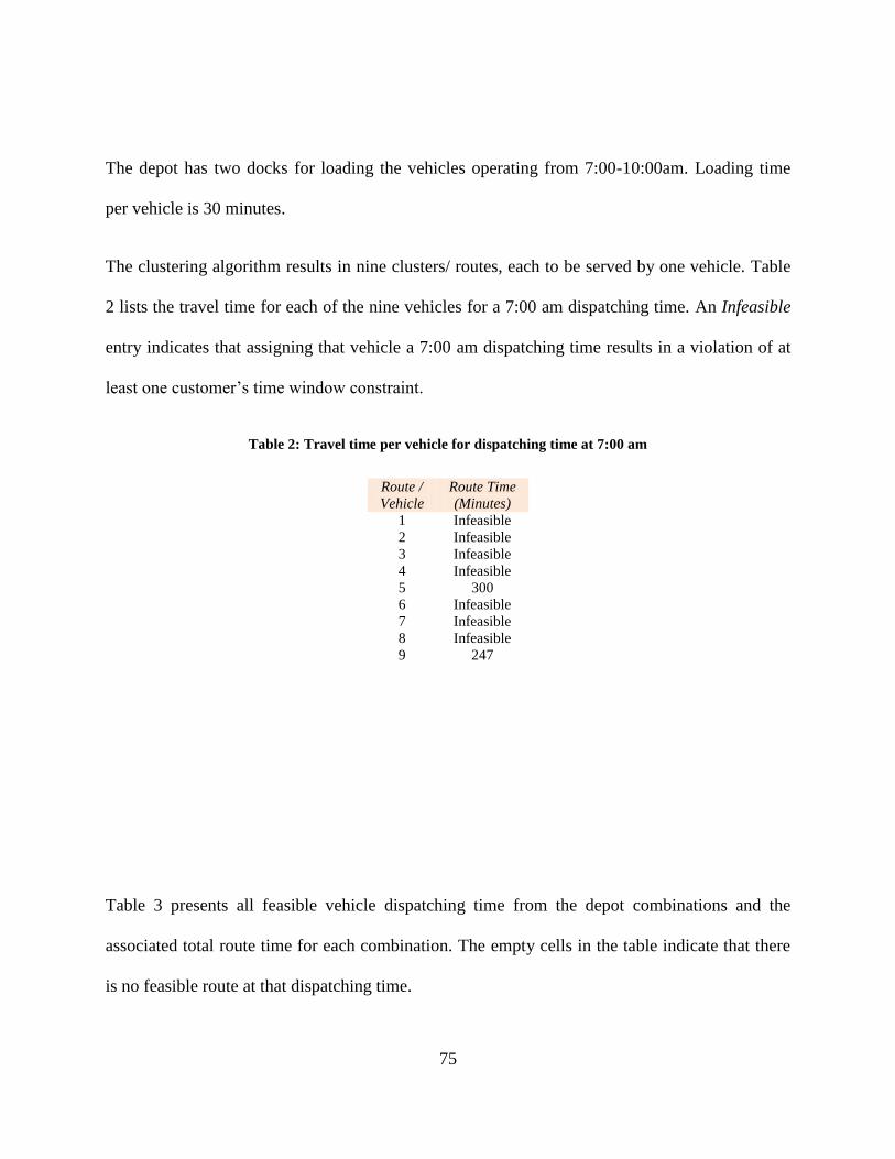
75
The depot has two docks for loading the vehicles operating from 7:00-10:00am. Loading time
per vehicle is 30 minutes.
The clustering algorithm results in nine clusters/ routes, each to be served by one vehicle. Table
2 lists the travel time for each of the nine vehicles for a 7:00 am dispatching time. An Infeasible
entry indicates that assigning that vehicle a 7:00 am dispatching time results in a violation of at
least one customer’s time window constraint.
Table 2: Travel time per vehicle for dispatching time at 7:00 am
Route /
Vehicle
Route Time
(Minutes)
1 Infeasible
2 Infeasible
3 Infeasible
4 Infeasible
5 300
6 Infeasible
7 Infeasible
8 Infeasible
9 247
Table 3 presents all feasible vehicle dispatching time from the depot combinations and the
associated total route time for each combination. The empty cells in the table indicate that there
is no feasible route at that dispatching time.

76
Table 3: Vehicle travel times for different dispatching times from the depot
Dock1 Dock2
7:00 7:30 8:00 8:30 9:00 9:30 10:00 7:00 7:30 8:00 8:30 9:00 9:30 10:00
1 2 3 4 5 6 7 8 9 10 11 12 13 14
Vehicle 1 292 292 290 290 292 292 290 290
Vehicle 2 207 201 207 201
Vehicle 3 236 236
Vehicle 4 273 243 231 273 243 231
Vehicle 5 300 288
288 288 288 288
300 288
288 288 288 288
Vehicle 6 281 278 269 269 269 281 278 269 269 269
Vehicle 7 226 223 226 223
Vehicle 8 352 367 352 367
Vehicle 9 247 181 172 175 175 247 181 172 175 175
Applying the Assignment Model Formulation to determine the best assignment of dispatching
times to vehicles results in the solution displayed in Table 4, where five vehicles are loaded from
Dock 1 during the period from 8:00am to 10:00am dispatching a vehicle every 30 minutes, while
Dock 2 dispatches four vehicles at 8:00am, 9:00am, 9:30am, and 10:00 am.
Table 4: Vehicle Loading, Dispatching and Dock Utilization.
Loading interval Dock #1 Dock #2
7:30-8:00 Vehicle/Route 9 Vehicle/Route 8
8:00-8:30 Vehicle/Route 5
8:30-9:00 Vehicle/Route 6 Vehicle/Route 1
9:00-9:30 Vehicle/Route 3 Vehicle/Route 2
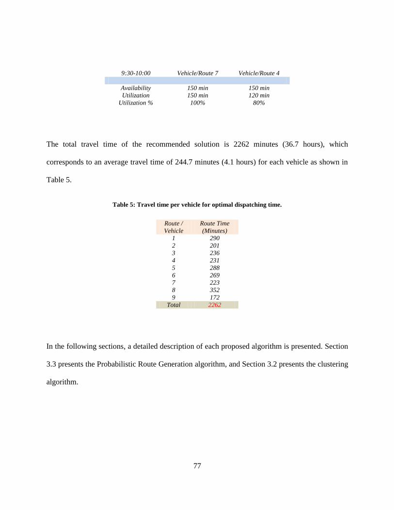
77
9:30-10:00 Vehicle/Route 7 Vehicle/Route 4
Availability 150 min 150 min
Utilization 150 min 120 min
Utilization % 100% 80%
The total travel time of the recommended solution is 2262 minutes (36.7 hours), which
corresponds to an average travel time of 244.7 minutes (4.1 hours) for each vehicle as shown in
Table 5.
Table 5: Travel time per vehicle for optimal dispatching time.
Route /
Vehicle
Route Time
(Minutes)
1 290
2 201
3 236
4 231
5 288
6 269
7 223
8 352
9 172
Total 2262
In the following sections, a detailed description of each proposed algorithm is presented. Section
3.3 presents the Probabilistic Route Generation algorithm, and Section 3.2 presents the clustering
algorithm.
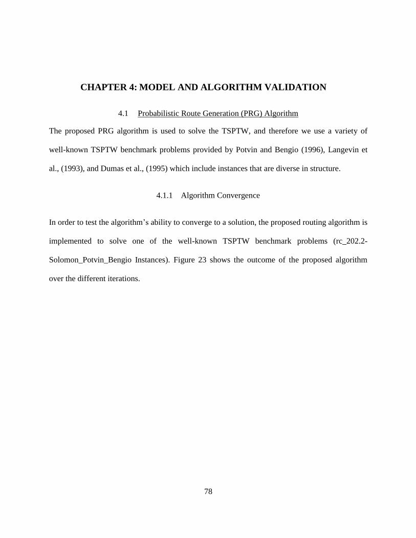
78
CHAPTER 4: MODEL AND ALGORITHM VALIDATION
4.1 Probabilistic Route Generation (PRG) Algorithm
The proposed PRG algorithm is used to solve the TSPTW, and therefore we use a variety of
well-known TSPTW benchmark problems provided by Potvin and Bengio (1996), Langevin et
al., (1993), and Dumas et al., (1995) which include instances that are diverse in structure.
4.1.1 Algorithm Convergence
In order to test the algorithm’s ability to converge to a solution, the proposed routing algorithm is
implemented to solve one of the well-known TSPTW benchmark problems (rc_202.2-
Solomon_Potvin_Bengio Instances). Figure 23 shows the outcome of the proposed algorithm
over the different iterations.
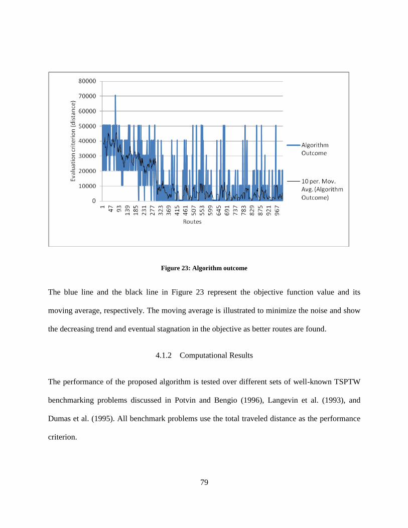
79
Figure 23: Algorithm outcome
The blue line and the black line in Figure 23 represent the objective function value and its
moving average, respectively. The moving average is illustrated to minimize the noise and show
the decreasing trend and eventual stagnation in the objective as better routes are found.
4.1.2 Computational Results
The performance of the proposed algorithm is tested over different sets of well-known TSPTW
benchmarking problems discussed in Potvin and Bengio (1996), Langevin et al. (1993), and
Dumas et al. (1995). All benchmark problems use the total traveled distance as the performance
criterion.
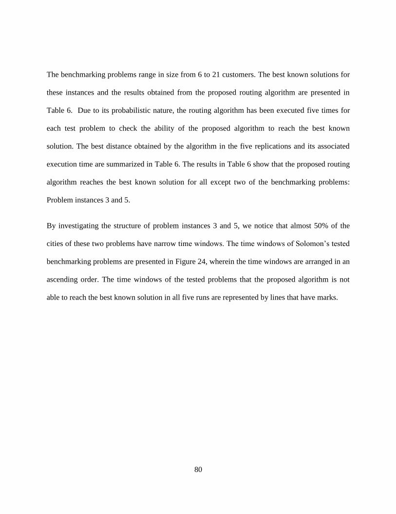
80
The benchmarking problems range in size from 6 to 21 customers. The best known solutions for
these instances and the results obtained from the proposed routing algorithm are presented in
Table 6. Due to its probabilistic nature, the routing algorithm has been executed five times for
each test problem to check the ability of the proposed algorithm to reach the best known
solution. The best distance obtained by the algorithm in the five replications and its associated
execution time are summarized in Table 6. The results in Table 6 show that the proposed routing
algorithm reaches the best known solution for all except two of the benchmarking problems:
Problem instances 3 and 5.
By investigating the structure of problem instances 3 and 5, we notice that almost 50% of the
cities of these two problems have narrow time windows. The time windows of Solomon’s tested
benchmarking problems are presented in Figure 24, wherein the time windows are arranged in an
ascending order. The time windows of the tested problems that the proposed algorithm is not
able to reach the best known solution in all five runs are represented by lines that have marks.
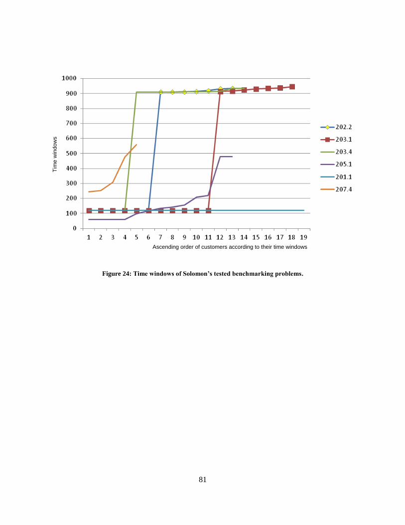
81
Ascending order of customers according to their time windows
Tim
e w
ind
ow
s
Figure 24: Time windows of Solomon’s tested benchmarking problems.
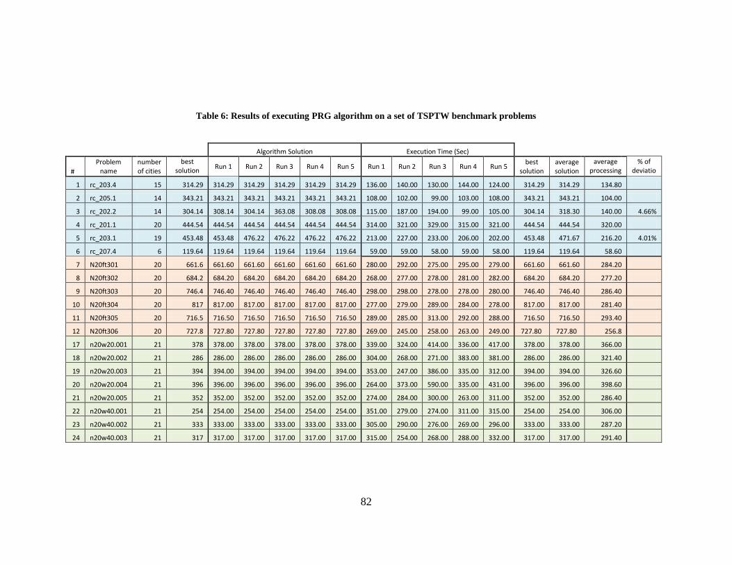
82
Table 6: Results of executing PRG algorithm on a set of TSPTW benchmark problems
Algorithm Solution Execution Time (Sec)
#
Problem name
number of cities
best solution known
Run 1 Run 2 Run 3 Run 4 Run 5 Run 1 Run 2 Run 3 Run 4 Run 5 best
solution average solution
average processing
time
% of deviatio
n 1 rc_203.4 15 314.29 314.29 314.29 314.29 314.29 314.29 136.00 140.00 130.00 144.00 124.00 314.29 314.29 134.80
2 rc_205.1 14 343.21 343.21 343.21 343.21 343.21 343.21 108.00 102.00 99.00 103.00 108.00 343.21 343.21 104.00
3 rc_202.2 14 304.14 308.14 304.14 363.08 308.08 308.08 115.00 187.00 194.00 99.00 105.00 304.14 318.30 140.00 4.66%
4 rc_201.1 20 444.54 444.54 444.54 444.54 444.54 444.54 314.00 321.00 329.00 315.00 321.00 444.54 444.54 320.00
5 rc_203.1 19 453.48 453.48 476.22 476.22 476.22 476.22 213.00 227.00 233.00 206.00 202.00 453.48 471.67 216.20 4.01%
6 rc_207.4 6 119.64 119.64 119.64 119.64 119.64 119.64 59.00 59.00 58.00 59.00 58.00 119.64 119.64 58.60
7 N20ft301 20 661.6 661.60 661.60 661.60 661.60 661.60 280.00 292.00 275.00 295.00 279.00 661.60 661.60 284.20
8 N20ft302 20 684.2 684.20 684.20 684.20 684.20 684.20 268.00 277.00 278.00 281.00 282.00 684.20 684.20 277.20
9 N20ft303 20 746.4 746.40 746.40 746.40 746.40 746.40 298.00 298.00 278.00 278.00 280.00 746.40 746.40 286.40
10 N20ft304 20 817 817.00 817.00 817.00 817.00 817.00 277.00 279.00 289.00 284.00 278.00 817.00 817.00 281.40
11 N20ft305 20 716.5 716.50 716.50 716.50 716.50 716.50 289.00 285.00 313.00 292.00 288.00 716.50 716.50 293.40
12 N20ft306 20 727.8 727.80 727.80 727.80 727.80 727.80 269.00 245.00 258.00 263.00 249.00 727.80 727.80 256.8
17 n20w20.001 21 378 378.00 378.00 378.00 378.00 378.00 339.00 324.00 414.00 336.00 417.00 378.00 378.00 366.00
18 n20w20.002 21 286 286.00 286.00 286.00 286.00 286.00 304.00 268.00 271.00 383.00 381.00 286.00 286.00 321.40
19 n20w20.003 21 394 394.00 394.00 394.00 394.00 394.00 353.00 247.00 386.00 335.00 312.00 394.00 394.00 326.60
20 n20w20.004 21 396 396.00 396.00 396.00 396.00 396.00 264.00 373.00 590.00 335.00 431.00 396.00 396.00 398.60
21 n20w20.005 21 352 352.00 352.00 352.00 352.00 352.00 274.00 284.00 300.00 263.00 311.00 352.00 352.00 286.40
22 n20w40.001 21 254 254.00 254.00 254.00 254.00 254.00 351.00 279.00 274.00 311.00 315.00 254.00 254.00 306.00
23 n20w40.002 21 333 333.00 333.00 333.00 333.00 333.00 305.00 290.00 276.00 269.00 296.00 333.00 333.00 287.20
24 n20w40.003 21 317 317.00 317.00 317.00 317.00 317.00 315.00 254.00 268.00 288.00 332.00 317.00 317.00 291.40
83
4.2 VRPTW Benchmark Problems
The performance of the proposed clustering and routing algorithms is tested over different sets of
known VRPTW benchmark problems like R, C, and RC problem instances generated by
Solomon (1987).
Solomon (1987) generates six sets of VRPTW benchmark problems to be used as a base for
testing the performance of the different algorithms. The design of these benchmark problems
considers several factors that can affect the performance of the routing and scheduling heuristics.
These factors include the following:
Geographical data
The number of customers serviced by a vehicle
The time window characteristics such as the percentage of time-constrained customers,
and narrowness and positioning of the time windows.
The customers’ coordinates and demand data used in generating the VRPTW benchmark
problems are based on the data for some of the problems from the standard set of routing test
problems given in Christofides et al. (1979).
The geographical data for the six VRPTW benchmark problem sets are randomly generated by:
Random uniform distribution (problem sets R1 and R2)
Clustered (problem sets C1 and C2)
Semi-clustered (problem sets RC1 and RC2), these sets of problems contain a mix of
randomly-generated data and clusters.

84
Problem sets R1, C1, and RC1 have narrow time windows and small vehicle capacity, which
allow only a few customers to be serviced by the same vehicle. In contrast, sets R2, C2 and RC2
have wide time windows and large vehicle capacities, which permit many customers to be
serviced by the same vehicle.
The time windows of the different problem sets are generated with various widths to achieve
different time window densities, defined as the percentages of customers with time windows,
specifically, 25, 50, 75, and 100% time window densities are observed in the benchmark
problems.
4.2.1 Computational Results
The proposed algorithm has been tested for R101-104, C101-104, and RC101-104 VRPTW
benchmark problems, and the best known solutions for these instances and the results obtained
from the proposed algorithm are summarized in Table 7.
The results presented in Table 7 show that the proposed algorithm is able to reach the best
documented solution with deviation ranges from 0.23% - 3.75% for C101-104 benchmark
problems. While for R101-104 benchmark problems, the deviation from the best known
solutions ranges from 7.12% - 27.70%. The deviation for RC101-104 benchmark problems is a
mix between the deviations for the C and R problems.
The percent deviation is influenced by the structure of the benchmark problem. In the C-type
problems the customers are clustered into groups, which enable the proposed clustering

85
algorithm to reach the best known solution with a very small deviation percentage. While in the
R-type problems the customers’ geographical locations are randomly generated resulting in
solutions that have wide-apart customers joining the same cluster.
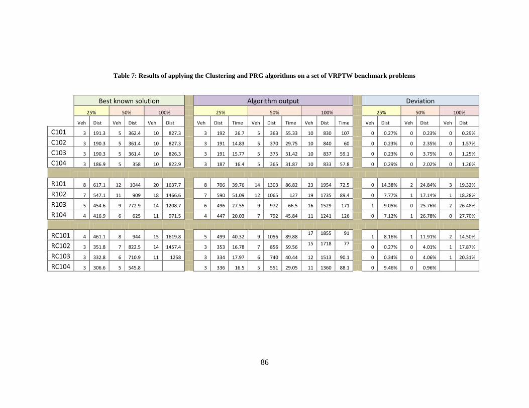
86
Table 7: Results of applying the Clustering and PRG algorithms on a set of VRPTW benchmark problems
Best known solution Algorithm output Deviation
25% 50% 100% 25% 50% 100% 25% 50% 100%
Veh Dist Veh Dist Veh Dist Veh Dist Time Veh Dist Time Veh Dist Time Veh Dist Veh Dist Veh Dist
C101 3 191.3 5 362.4 10 827.3 3 192 26.7 5 363 55.33 10 830 107 0 0.27% 0 0.23% 0 0.29%
C102 3 190.3 5 361.4 10 827.3 3 191 14.83 5 370 29.75 10 840 60 0 0.23% 0 2.35% 0 1.57%
C103 3 190.3 5 361.4 10 826.3 3 191 15.77 5 375 31.42 10 837 59.1 0 0.23% 0 3.75% 0 1.25%
C104 3 186.9 5 358 10 822.9 3 187 16.4 5 365 31.87 10 833 57.8 0 0.29% 0 2.02% 0 1.26%
R101 8 617.1 12 1044 20 1637.7 8 706 39.76 14 1303 86.82 23 1954 72.5 0 14.38% 2 24.84% 3 19.32%
R102 7 547.1 11 909 18 1466.6 7 590 51.09 12 1065 127 19 1735 89.4 0 7.77% 1 17.14% 1 18.28%
R103 5 454.6 9 772.9 14 1208.7 6 496 27.55 9 972 66.5 16 1529 171 1 9.05% 0 25.76% 2 26.48%
R104 4 416.9 6 625 11 971.5 4 447 20.03 7 792 45.84 11 1241 126 0 7.12% 1 26.78% 0 27.70%
RC101 4 461.1 8 944 15 1619.8 5 499 40.32 9 1056 89.88 17 1855 91
1 8.16% 1 11.91% 2 14.50%
RC102 3 351.8 7 822.5 14 1457.4 3 353 16.78 7 856 59.56 15 1718 77
0 0.27% 0 4.01% 1 17.87%
RC103 3 332.8 6 710.9 11 1258 3 334 17.97 6 740 40.44 12 1513 90.1 0 0.34% 0 4.06% 1 20.31%
RC104 3 306.6 5 545.8 3 336 16.5 5 551 29.05 11 1360 88.1 0 9.46% 0 0.96%

87
CHAPTER 5: VRPTW BENCHMAK PROBLEMS MODIFICATION AND
TESTING
In the previous chapter, the performance of the proposed Clustering and Routing algorithms is
evaluated over a set of VRPTW benchmark problems. To the best of our knowledge, there are no
benchmark problems for the VRPTW variant studied in this research which includes two
additional constraints enforcing the earlier limit of the time windows and the limited dock
dispatching capacity. Therefore, in this chapter we first modify some of the existing VRPTW
benchmark problems to accommodate the two extra constraints. Then, we demonstrate the three
proposed algorithms of Clustering, Routing, and Assignment by applying them to the modified
benchmark problems.
5.1 VRPTW Benchmark Problems Structure
Figure 25 illustrates the structure of the well known VRPTW benchmark problems discussed in
Section 4.2. Each customer in the problem is characterized by four main characteristics. The first
characteristic is the geographical structure of the customers (X & Y coordinates) that determines
the relative distance between each customer.
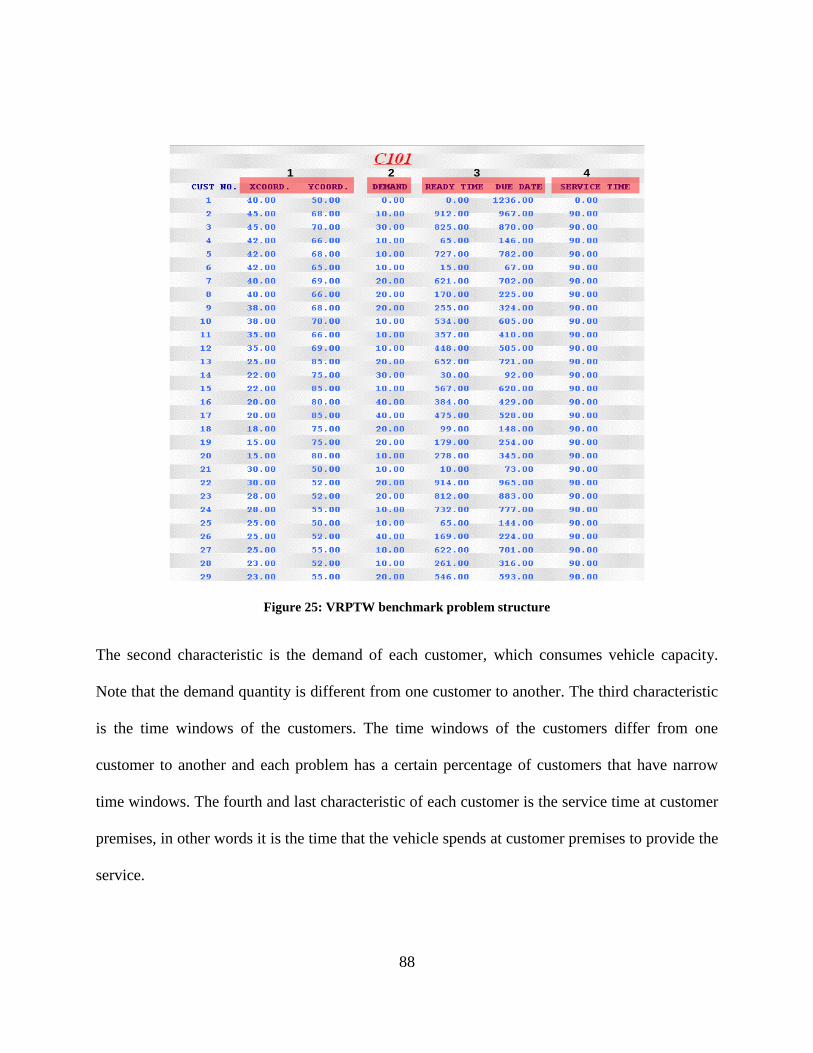
88
1 2 3 4
Figure 25: VRPTW benchmark problem structure
The second characteristic is the demand of each customer, which consumes vehicle capacity.
Note that the demand quantity is different from one customer to another. The third characteristic
is the time windows of the customers. The time windows of the customers differ from one
customer to another and each problem has a certain percentage of customers that have narrow
time windows. The fourth and last characteristic of each customer is the service time at customer
premises, in other words it is the time that the vehicle spends at customer premises to provide the
service.
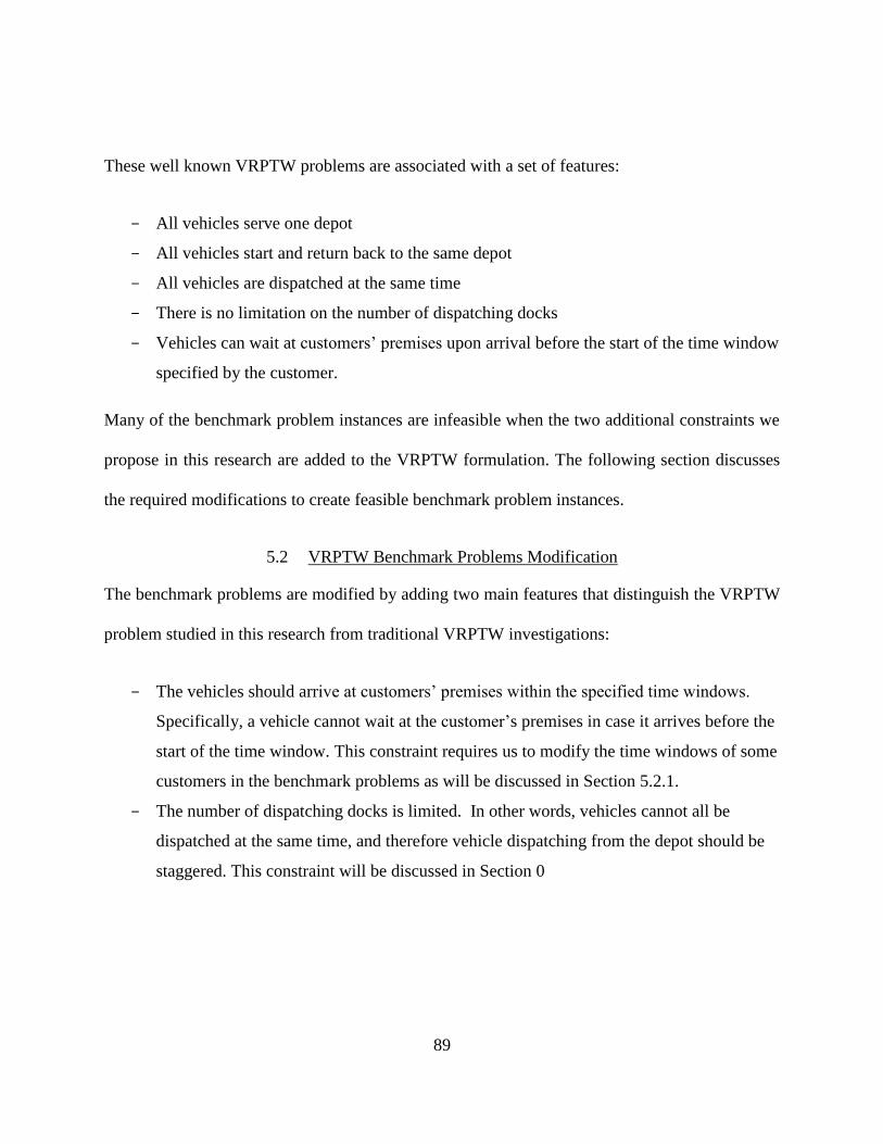
89
These well known VRPTW problems are associated with a set of features:
All vehicles serve one depot
All vehicles start and return back to the same depot
All vehicles are dispatched at the same time
There is no limitation on the number of dispatching docks
Vehicles can wait at customers’ premises upon arrival before the start of the time window
specified by the customer.
Many of the benchmark problem instances are infeasible when the two additional constraints we
propose in this research are added to the VRPTW formulation. The following section discusses
the required modifications to create feasible benchmark problem instances.
5.2 VRPTW Benchmark Problems Modification
The benchmark problems are modified by adding two main features that distinguish the VRPTW
problem studied in this research from traditional VRPTW investigations:
The vehicles should arrive at customers’ premises within the specified time windows.
Specifically, a vehicle cannot wait at the customer’s premises in case it arrives before the
start of the time window. This constraint requires us to modify the time windows of some
customers in the benchmark problems as will be discussed in Section 5.2.1.
The number of dispatching docks is limited. In other words, vehicles cannot all be
dispatched at the same time, and therefore vehicle dispatching from the depot should be
staggered. This constraint will be discussed in Section 0
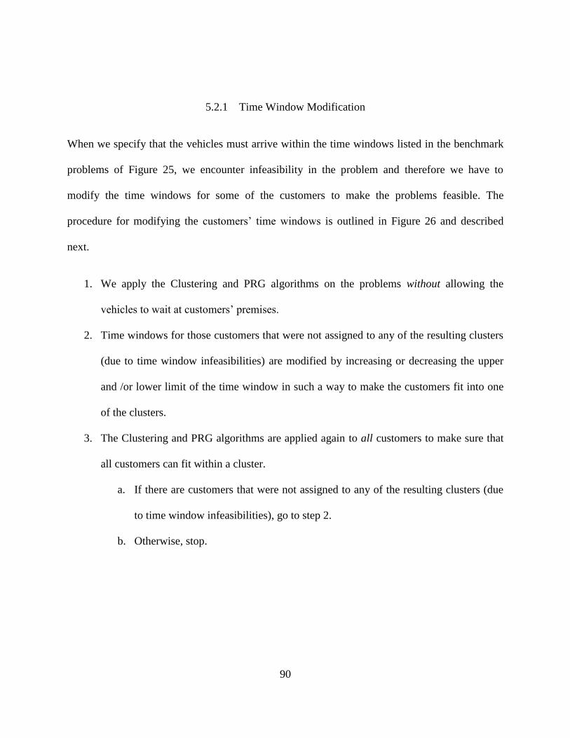
90
5.2.1 Time Window Modification
When we specify that the vehicles must arrive within the time windows listed in the benchmark
problems of Figure 25, we encounter infeasibility in the problem and therefore we have to
modify the time windows for some of the customers to make the problems feasible. The
procedure for modifying the customers’ time windows is outlined in Figure 26 and described
next.
1. We apply the Clustering and PRG algorithms on the problems without allowing the
vehicles to wait at customers’ premises.
2. Time windows for those customers that were not assigned to any of the resulting clusters
(due to time window infeasibilities) are modified by increasing or decreasing the upper
and /or lower limit of the time window in such a way to make the customers fit into one
of the clusters.
3. The Clustering and PRG algorithms are applied again to all customers to make sure that
all customers can fit within a cluster.
a. If there are customers that were not assigned to any of the resulting clusters (due
to time window infeasibilities), go to step 2.
b. Otherwise, stop.
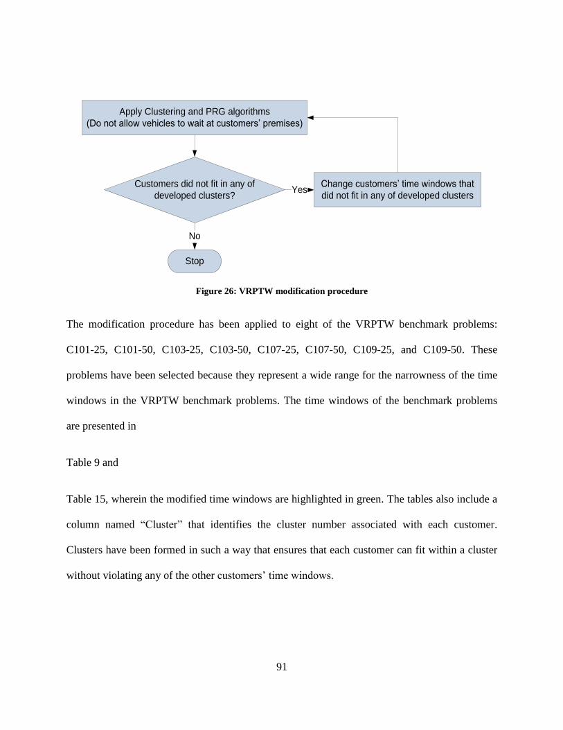
91
Apply Clustering and PRG algorithms
(Do not allow vehicles to wait at customers’ premises)
Customers did not fit in any of
developed clusters?
Change customers’ time windows that
did not fit in any of developed clusters Yes
Stop
No
Figure 26: VRPTW modification procedure
The modification procedure has been applied to eight of the VRPTW benchmark problems:
C101-25, C101-50, C103-25, C103-50, C107-25, C107-50, C109-25, and C109-50. These
problems have been selected because they represent a wide range for the narrowness of the time
windows in the VRPTW benchmark problems. The time windows of the benchmark problems
are presented in
Table 9 and
Table 15, wherein the modified time windows are highlighted in green. The tables also include a
column named “Cluster” that identifies the cluster number associated with each customer.
Clusters have been formed in such a way that ensures that each customer can fit within a cluster
without violating any of the other customers’ time windows.
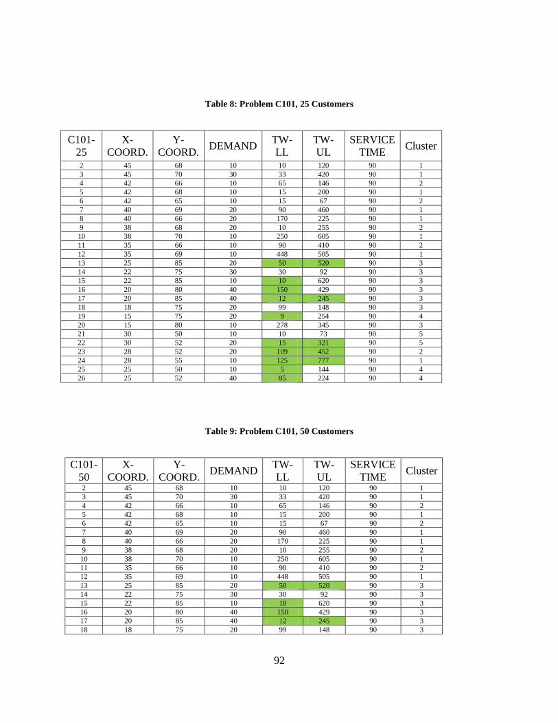
92
Table 8: Problem C101, 25 Customers
C101-
25
X-
COORD.
Y-
COORD. DEMAND
TW-
LL
TW-
UL
SERVICE
TIME Cluster
2 45 68 10 10 120 90 1
3 45 70 30 33 420 90 1
4 42 66 10 65 146 90 2
5 42 68 10 15 200 90 1
6 42 65 10 15 67 90 2
7 40 69 20 90 460 90 1
8 40 66 20 170 225 90 1
9 38 68 20 10 255 90 2
10 38 70 10 250 605 90 1
11 35 66 10 90 410 90 2
12 35 69 10 448 505 90 1
13 25 85 20 50 520 90 3
14 22 75 30 30 92 90 3
15 22 85 10 10 620 90 3
16 20 80 40 150 429 90 3
17 20 85 40 12 245 90 3
18 18 75 20 99 148 90 3
19 15 75 20 9 254 90 4
20 15 80 10 278 345 90 3
21 30 50 10 10 73 90 5
22 30 52 20 15 321 90 5
23 28 52 20 109 452 90 2
24 28 55 10 125 777 90 1
25 25 50 10 5 144 90 4
26 25 52 40 85 224 90 4
Table 9: Problem C101, 50 Customers
C101-
50
X-
COORD.
Y-
COORD. DEMAND
TW-
LL
TW-
UL
SERVICE
TIME Cluster
2 45 68 10 10 120 90 1
3 45 70 30 33 420 90 1
4 42 66 10 65 146 90 2
5 42 68 10 15 200 90 1
6 42 65 10 15 67 90 2
7 40 69 20 90 460 90 1
8 40 66 20 170 225 90 1
9 38 68 20 10 255 90 2
10 38 70 10 250 605 90 1
11 35 66 10 90 410 90 2
12 35 69 10 448 505 90 1
13 25 85 20 50 520 90 3
14 22 75 30 30 92 90 3
15 22 85 10 10 620 90 3
16 20 80 40 150 429 90 3
17 20 85 40 12 245 90 3
18 18 75 20 99 148 90 3
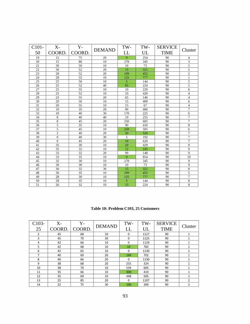
93
C101-
50
X-
COORD.
Y-
COORD. DEMAND
TW-
LL
TW-
UL
SERVICE
TIME Cluster
19 15 75 20 9 254 90 4
20 15 80 10 278 345 90 3
21 30 50 10 10 73 90 5
22 30 52 20 15 321 90 5
23 28 52 20 109 452 90 2
24 28 55 10 125 777 90 1
25 25 50 10 5 144 90 5
26 25 52 40 85 224 90 5
27 25 55 10 10 220 90 6
28 23 52 10 33 420 90 4
29 23 55 20 65 146 90 4
30 20 50 10 15 400 90 6
31 20 55 10 15 67 90 4
32 10 35 20 90 460 90 7
33 10 40 30 170 225 90 6
34 8 40 40 10 255 90 7
35 8 45 20 250 605 90 7
36 5 35 10 90 410 90 8
37 5 45 10 250 505 90 6
38 2 40 20 50 520 90 7
39 0 40 30 5 192 90 7
40 0 45 20 10 620 90 7
41 35 30 10 20 429 90 9
42 35 32 10 12 245 90 9
43 33 32 20 99 148 90 9
44 33 35 10 9 854 90 10
45 32 30 10 278 345 90 9
46 30 30 10 10 73 90 9
47 30 32 30 15 321 90 8
48 30 35 10 109 452 90 5
49 28 30 10 125 777 90 7
50 28 35 10 5 144 90 8
51 26 32 10 15 224 90 8
Table 10: Problem C103, 25 Customers
C103-
25
X-
COORD.
Y-
COORD. DEMAND
TW-
LL
TW-
UL
SERVICE
TIME Cluster
2 45 68 10 0 1127 90 1
3 45 70 30 0 1125 90 1
4 42 66 10 0 1129 90 1
5 42 68 10 10 782 90 1
6 42 65 10 0 1130 90 1
7 40 69 20 169 702 90 1
8 40 66 20 0 1130 90 1
9 38 68 20 255 324 90 1
10 38 70 10 534 605 90 1
11 35 66 10 300 410 90 1
12 35 69 10 448 505 90 1
13 25 85 20 0 1107 90 2
14 22 75 30 100 300 90 2
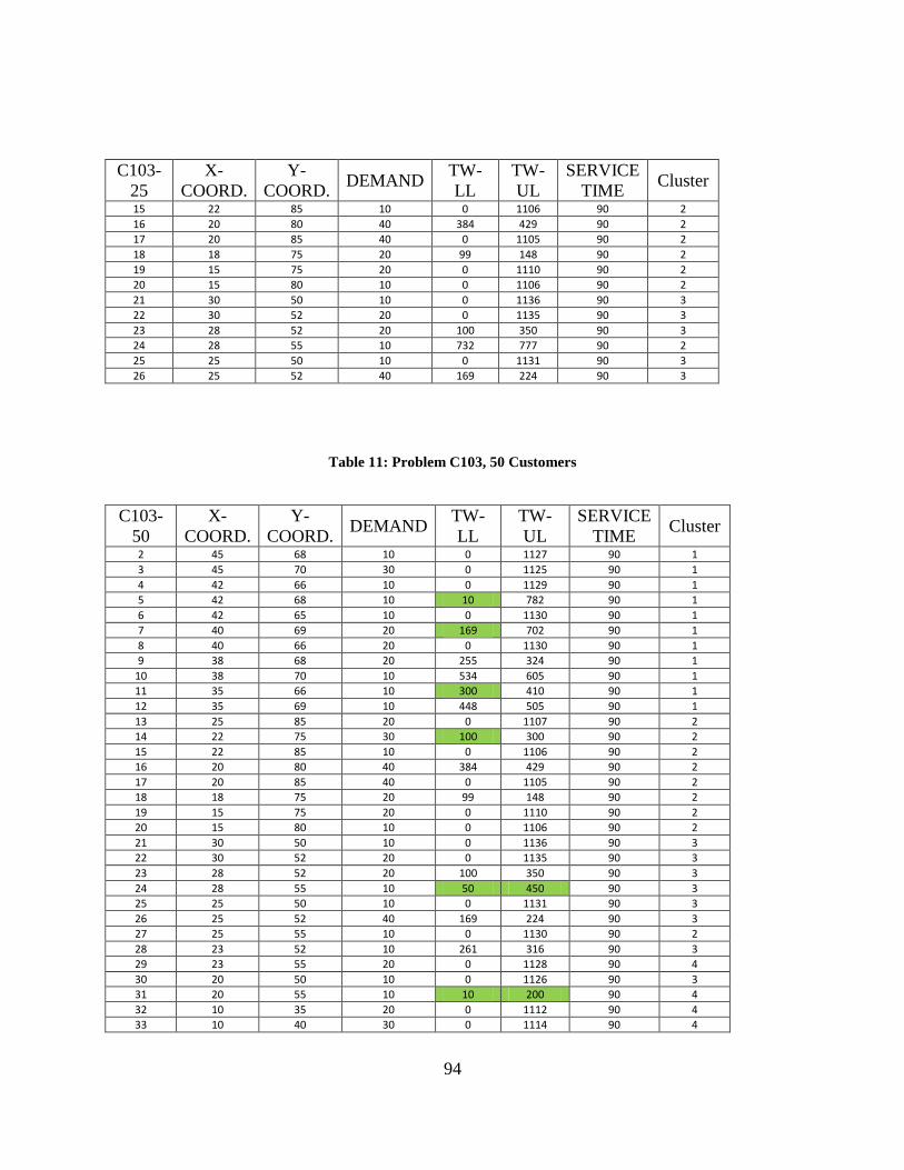
94
C103-
25
X-
COORD.
Y-
COORD. DEMAND
TW-
LL
TW-
UL
SERVICE
TIME Cluster
15 22 85 10 0 1106 90 2
16 20 80 40 384 429 90 2
17 20 85 40 0 1105 90 2
18 18 75 20 99 148 90 2
19 15 75 20 0 1110 90 2
20 15 80 10 0 1106 90 2
21 30 50 10 0 1136 90 3
22 30 52 20 0 1135 90 3
23 28 52 20 100 350 90 3
24 28 55 10 732 777 90 2
25 25 50 10 0 1131 90 3
26 25 52 40 169 224 90 3
Table 11: Problem C103, 50 Customers
C103-
50
X-
COORD.
Y-
COORD. DEMAND
TW-
LL
TW-
UL
SERVICE
TIME Cluster
2 45 68 10 0 1127 90 1
3 45 70 30 0 1125 90 1
4 42 66 10 0 1129 90 1
5 42 68 10 10 782 90 1
6 42 65 10 0 1130 90 1
7 40 69 20 169 702 90 1
8 40 66 20 0 1130 90 1
9 38 68 20 255 324 90 1
10 38 70 10 534 605 90 1
11 35 66 10 300 410 90 1
12 35 69 10 448 505 90 1
13 25 85 20 0 1107 90 2
14 22 75 30 100 300 90 2
15 22 85 10 0 1106 90 2
16 20 80 40 384 429 90 2
17 20 85 40 0 1105 90 2
18 18 75 20 99 148 90 2
19 15 75 20 0 1110 90 2
20 15 80 10 0 1106 90 2
21 30 50 10 0 1136 90 3
22 30 52 20 0 1135 90 3
23 28 52 20 100 350 90 3
24 28 55 10 50 450 90 3
25 25 50 10 0 1131 90 3
26 25 52 40 169 224 90 3
27 25 55 10 0 1130 90 2
28 23 52 10 261 316 90 3
29 23 55 20 0 1128 90 4
30 20 50 10 0 1126 90 3
31 20 55 10 10 200 90 4
32 10 35 20 0 1112 90 4
33 10 40 30 0 1114 90 4
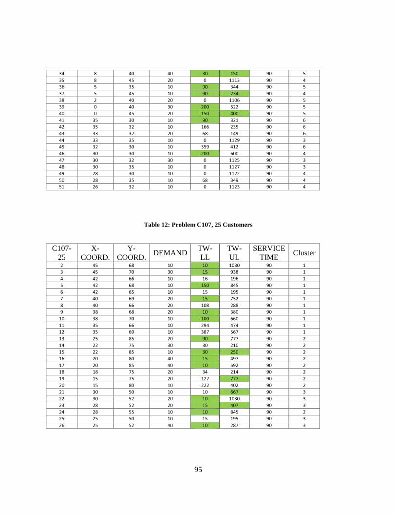
95
34 8 40 40 30 150 90 5
35 8 45 20 0 1113 90 4
36 5 35 10 90 344 90 5
37 5 45 10 90 234 90 4
38 2 40 20 0 1106 90 5
39 0 40 30 200 522 90 5
40 0 45 20 150 400 90 5
41 35 30 10 90 321 90 6
42 35 32 10 166 235 90 6
43 33 32 20 68 149 90 6
44 33 35 10 0 1129 90 3
45 32 30 10 359 412 90 6
46 30 30 10 200 600 90 4
47 30 32 30 0 1125 90 3
48 30 35 10 0 1127 90 3
49 28 30 10 0 1122 90 4
50 28 35 10 68 349 90 4
51 26 32 10 0 1123 90 4
Table 12: Problem C107, 25 Customers
C107-
25
X-
COORD.
Y-
COORD. DEMAND
TW-
LL
TW-
UL
SERVICE
TIME Cluster
2 45 68 10 10 1030 90 1
3 45 70 30 15 938 90 1
4 42 66 10 16 196 90 1
5 42 68 10 150 845 90 1
6 42 65 10 15 195 90 1
7 40 69 20 15 752 90 1
8 40 66 20 108 288 90 1
9 38 68 20 10 380 90 1
10 38 70 10 100 660 90 1
11 35 66 10 294 474 90 1
12 35 69 10 387 567 90 1
13 25 85 20 90 777 90 2
14 22 75 30 30 210 90 2
15 22 85 10 30 250 90 2
16 20 80 40 15 497 90 2
17 20 85 40 10 592 90 2
18 18 75 20 34 214 90 2
19 15 75 20 127 777 90 2
20 15 80 10 222 402 90 2
21 30 50 10 10 667 90 3
22 30 52 20 10 1030 90 3
23 28 52 20 15 407 90 3
24 28 55 10 10 845 90 2
25 25 50 10 15 195 90 3
26 25 52 40 10 287 90 3
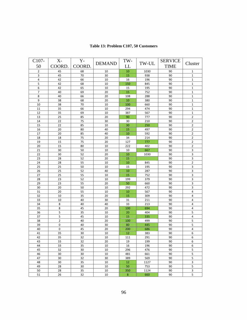
96
Table 13: Problem C107, 50 Customers
C107-
50
X-
COORD.
Y-
COORD. DEMAND
TW-
LL TW-UL
SERVICE
TIME Cluster
2 45 68 10 10 1030 90 1
3 45 70 30 15 938 90 1
4 42 66 10 16 196 90 1
5 42 68 10 150 845 90 1
6 42 65 10 15 195 90 1
7 40 69 20 15 752 90 1
8 40 66 20 108 288 90 1
9 38 68 20 10 380 90 1
10 38 70 10 100 660 90 1
11 35 66 10 294 474 90 1
12 35 69 10 387 567 90 1
13 25 85 20 90 777 90 2
14 22 75 30 30 210 90 2
15 22 85 10 30 250 90 2
16 20 80 40 15 497 90 2
17 20 85 40 10 592 90 2
18 18 75 20 34 214 90 2
19 15 75 20 127 777 90 2
20 15 80 10 222 402 90 2
21 30 50 10 10 667 90 3
22 30 52 20 10 1030 90 3
23 28 52 20 15 407 90 3
24 28 55 10 10 845 90 2
25 25 50 10 15 195 90 3
26 25 52 40 10 287 90 3
27 25 55 10 15 752 90 3
28 23 52 10 199 379 90 3
29 23 55 20 50 660 90 3
30 20 50 10 292 472 90 3
31 20 55 10 10 567 90 4
32 10 35 20 15 309 90 4
33 10 40 30 31 211 90 4
34 8 40 40 33 213 90 4
35 8 45 20 100 694 90 4
36 5 35 10 20 404 90 5
37 5 45 10 15 335 90 4
38 2 40 20 100 499 90 5
39 0 40 30 80 445 90 5
40 0 45 20 200 686 90 4
41 35 30 10 12 383 90 6
42 35 32 10 111 291 90 6
43 33 32 20 19 199 90 6
44 33 35 10 16 196 90 6
45 32 30 10 296 476 90 5
46 30 30 10 481 661 90 5
47 30 32 30 389 569 90 5
48 30 35 10 12 1127 90 3
49 28 30 10 50 753 90 5
50 28 35 10 350 1124 90 3
51 26 32 10 8 660 90 5
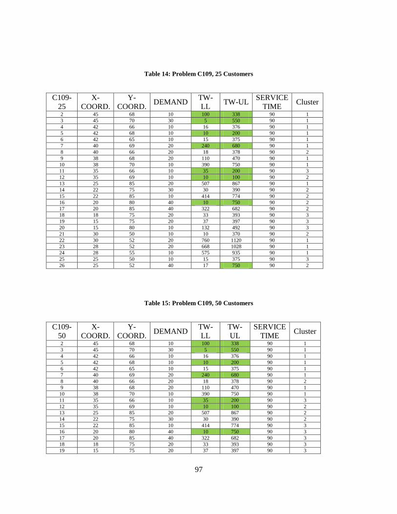
97
Table 14: Problem C109, 25 Customers
C109-
25
X-
COORD.
Y-
COORD. DEMAND
TW-
LL TW-UL
SERVICE
TIME Cluster
2 45 68 10 100 338 90 1
3 45 70 30 5 550 90 1
4 42 66 10 16 376 90 1
5 42 68 10 10 200 90 1
6 42 65 10 15 375 90 1
7 40 69 20 240 680 90 1
8 40 66 20 18 378 90 2
9 38 68 20 110 470 90 1
10 38 70 10 390 750 90 1
11 35 66 10 35 200 90 3
12 35 69 10 10 100 90 2
13 25 85 20 507 867 90 1
14 22 75 30 30 390 90 2
15 22 85 10 414 774 90 2
16 20 80 40 10 750 90 2
17 20 85 40 322 682 90 2
18 18 75 20 33 393 90 3
19 15 75 20 37 397 90 3
20 15 80 10 132 492 90 3
21 30 50 10 10 370 90 2
22 30 52 20 760 1120 90 1
23 28 52 20 668 1028 90 1
24 28 55 10 575 935 90 1
25 25 50 10 15 375 90 3
26 25 52 40 17 750 90 2
Table 15: Problem C109, 50 Customers
C109-
50
X-
COORD.
Y-
COORD. DEMAND
TW-
LL
TW-
UL
SERVICE
TIME Cluster
2 45 68 10 100 338 90 1
3 45 70 30 5 550 90 1
4 42 66 10 16 376 90 1
5 42 68 10 10 200 90 1
6 42 65 10 15 375 90 1
7 40 69 20 240 680 90 1
8 40 66 20 18 378 90 2
9 38 68 20 110 470 90 1
10 38 70 10 390 750 90 1
11 35 66 10 35 200 90 3
12 35 69 10 10 100 90 2
13 25 85 20 507 867 90 2
14 22 75 30 30 390 90 2
15 22 85 10 414 774 90 3
16 20 80 40 10 750 90 3
17 20 85 40 322 682 90 3
18 18 75 20 33 393 90 3
19 15 75 20 37 397 90 3
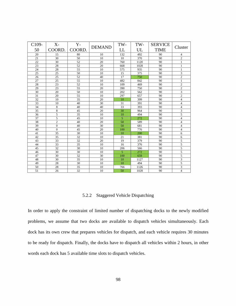
98
C109-
50
X-
COORD.
Y-
COORD. DEMAND
TW-
LL
TW-
UL
SERVICE
TIME Cluster
20 15 80 10 132 492 90 4
21 30 50 10 10 370 90 2
22 30 52 20 760 1120 90 1
23 28 52 20 668 1028 90 1
24 28 55 10 575 935 90 1
25 25 50 10 15 375 90 3
26 25 52 40 17 750 90 2
27 25 55 10 482 842 90 1
28 23 52 10 109 469 90 2
29 23 55 20 390 750 90 2
30 20 50 10 202 562 90 3
31 20 55 10 297 657 90 2
32 10 35 20 10 399 90 4
33 10 40 30 31 391 90 4
34 8 40 40 33 393 90 4
35 8 45 20 30 964 90 3
36 5 35 10 10 494 90 5
37 5 45 10 5 272 90 4
38 2 40 20 50 589 90 4
39 0 40 30 50 681 90 4
40 0 45 20 100 776 90 4
41 35 30 10 10 200 90 6
42 35 32 10 21 381 90 6
43 33 32 20 19 379 90 5
44 33 35 10 16 376 90 5
45 32 30 10 206 566 90 5
46 30 30 10 5 272 90 5
47 30 32 30 100 659 90 5
48 30 35 10 10 1127 90 3
49 28 30 10 10 494 90 5
50 28 35 10 766 1126 90 3
51 26 32 10 50 1028 90 4
5.2.2 Staggered Vehicle Dispatching
In order to apply the constraint of limited number of dispatching docks to the newly modified
problems, we assume that two docks are available to dispatch vehicles simultaneously. Each
dock has its own crew that prepares vehicles for dispatch, and each vehicle requires 30 minutes
to be ready for dispatch. Finally, the docks have to dispatch all vehicles within 2 hours, in other
words each dock has 5 available time slots to dispatch vehicles.
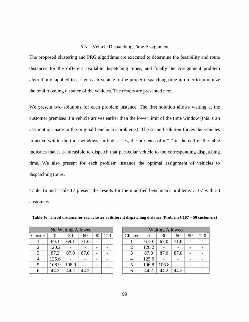
99
5.3 Vehicle Dispatching Time Assignment
The proposed clustering and PRG algorithms are executed to determine the feasibility and route
distances for the different available dispatching times, and finally the Assignment problem
algorithm is applied to assign each vehicle to the proper dispatching time in order to minimize
the total traveling distance of the vehicles. The results are presented next.
We present two solutions for each problem instance. The first solution allows waiting at the
customer premises if a vehicle arrives earlier than the lower limit of the time window (this is an
assumption made in the original benchmark problems). The second solution forces the vehicles
to arrive within the time windows. In both cases, the presence of a “-“ in the cell of the table
indicates that it is infeasible to dispatch that particular vehicle to the corresponding dispatching
time. We also present for each problem instance the optimal assignment of vehicles to
dispatching times.
Table 16 and Table 17 present the results for the modified benchmark problems C107 with 50
customers.
Table 16: Travel distance for each cluster at different dispatching distance (Problem C107 – 50 customers)
No Waiting Allowed
Waiting Allowed
Cluster 0 30 60 90 120
Cluster 0 30 60 90 120
1 69.1 69.1 71.6 - -
1 67.0 67.0 71.6 - -
2 120.2 - - - -
2 120.2 - - - -
3 87.3 87.0 87.0 - -
3 87.0 87.0 87.0 - -
4 125.6 - - - -
4 125.6 - - - -
5 108.9 108.9 - - -
5 106.8 106.8 - - -
6 44.2 44.2 44.2 - -
6 44.2 44.2 44.2 - -
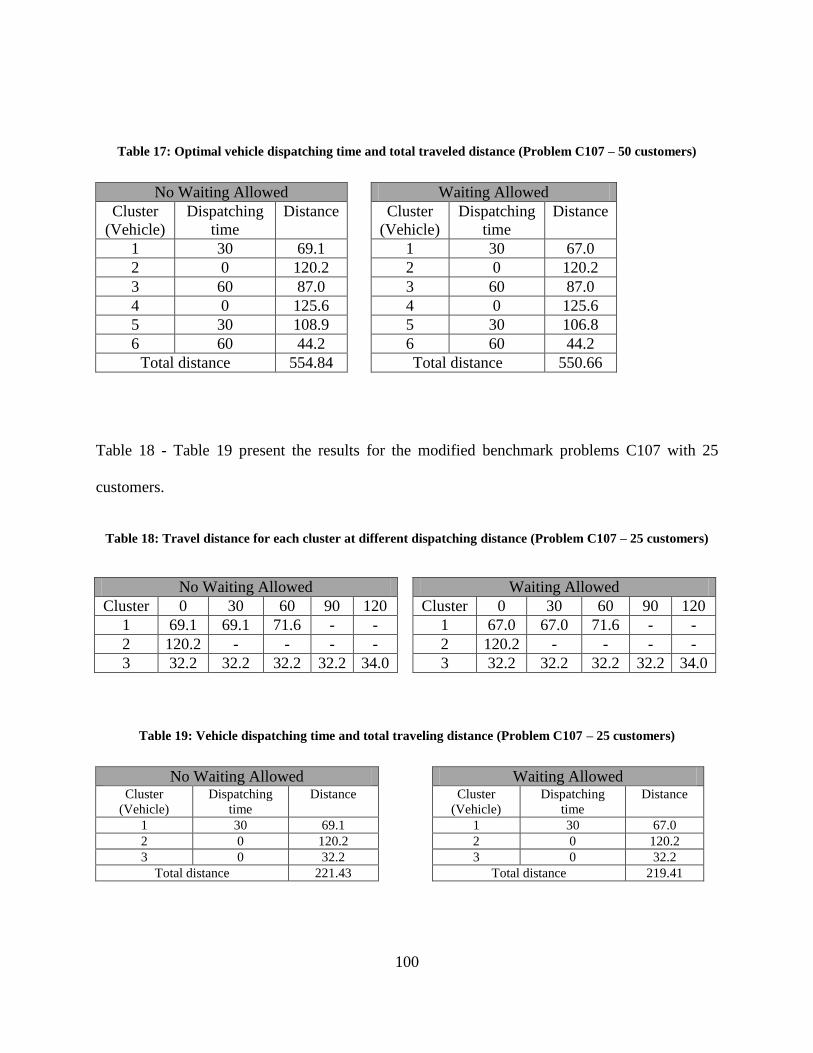
100
Table 17: Optimal vehicle dispatching time and total traveled distance (Problem C107 – 50 customers)
No Waiting Allowed Waiting Allowed
Cluster
(Vehicle)
Dispatching
time
Distance Cluster
(Vehicle)
Dispatching
time
Distance
1 30 69.1 1 30 67.0
2 0 120.2 2 0 120.2
3 60 87.0 3 60 87.0
4 0 125.6 4 0 125.6
5 30 108.9 5 30 106.8
6 60 44.2 6 60 44.2
Total distance 554.84 Total distance 550.66
Table 18 - Table 19 present the results for the modified benchmark problems C107 with 25
customers.
Table 18: Travel distance for each cluster at different dispatching distance (Problem C107 – 25 customers)
No Waiting Allowed
Waiting Allowed
Cluster 0 30 60 90 120
Cluster 0 30 60 90 120
1 69.1 69.1 71.6 - -
1 67.0 67.0 71.6 - -
2 120.2 - - - -
2 120.2 - - - -
3 32.2 32.2 32.2 32.2 34.0
3 32.2 32.2 32.2 32.2 34.0
Table 19: Vehicle dispatching time and total traveling distance (Problem C107 – 25 customers)
No Waiting Allowed Waiting Allowed Cluster
(Vehicle)
Dispatching
time
Distance Cluster
(Vehicle)
Dispatching
time
Distance
1 30 69.1 1 30 67.0
2 0 120.2 2 0 120.2
3 0 32.2 3 0 32.2
Total distance 221.43 Total distance 219.41
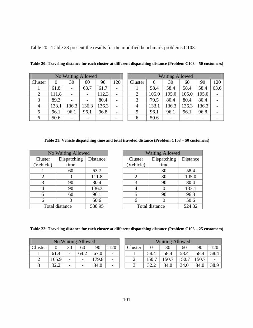
101
Table 20 - Table 23 present the results for the modified benchmark problems C103.
Table 20: Traveling distance for each cluster at different dispatching distance (Problem C103 – 50 customers)
No Waiting Allowed
Waiting Allowed
Cluster 0 30 60 90 120
Cluster 0 30 60 90 120
1 61.8 - 63.7 61.7 -
1 58.4 58.4 58.4 58.4 63.6
2 111.8 - - 112.3 -
2 105.0 105.0 105.0 105.0 -
3 89.3 - - 80.4 -
3 79.5 80.4 80.4 80.4 -
4 133.1 136.3 136.3 136.3 -
4 133.1 136.3 136.3 136.3 -
5 96.1 96.1 96.1 96.8 -
5 96.1 96.1 96.1 96.8 -
6 50.6 - - - -
6 50.6 - - - -
Table 21: Vehicle dispatching time and total traveled distance (Problem C103 – 50 customers)
No Waiting Allowed Waiting Allowed
Cluster
(Vehicle)
Dispatching
time
Distance Cluster
(Vehicle)
Dispatching
time
Distance
1 60 63.7 1 30 58.4
2 0 111.8 2 30 105.0
3 90 80.4 3 90 80.4
4 90 136.3 4 0 133.1
5 60 96.1 5 90 96.8
6 0 50.6 6 0 50.6
Total distance 538.95 Total distance 524.32
Table 22: Traveling distance for each cluster at different dispatching distance (Problem C103 – 25 customers)
No Waiting Allowed
Waiting Allowed
Cluster 0 30 60 90 120
Cluster 0 30 60 90 120
1 61.4 - 64.2 67.0 -
1 58.4 58.4 58.4 58.4 58.4
2 165.9 - - 179.8 -
2 150.7 150.7 150.7 150.7 -
3 32.2 - - 34.0 -
3 32.2 34.0 34.0 34.0 38.9

102
Table 23: Vehicle dispatching time and total traveled distance (Problem C103 – 25 customers)
No Waiting Allowed Waiting Allowed
Cluster
(Vehicle)
Dispatching
time
Distance Cluster
(Vehicle)
Dispatching
time
Distance
1 60 64.2 1 0 58.4
2 30 165.9 2 30 150.7
3 30 32.2 3 0 32.2
Total distance 262.25 Total distance 241.28
Table 24 - Table 27 present the results for the modified benchmark problems C101.
Table 24: Traveling distance for each cluster at different dispatching distance (Problem C101 – 50 customers)
No Waiting Allowed
Waiting Allowed
Cluster 0 30 60 90 120
Cluster 0 30 60 90 120
1 75.2 - - - -
1 75.2 - - - -
2 52.0 52.0 - - -
2 52.0 52.0 - - -
3 106.5 - - - -
3 106.5 - - - -
4 86.6 - - - -
4 86.6 - - - -
5 57.0 - - - -
5 57.0 - - - -
6 79.5 - 79.9 102.3 -
6 79.5 79.9 79.9 102.3 -
7 119.9 119.9 123.4 134.9 -
7 119.9 119.9 123.4 134.9 -
8 86.1 90.1 90.1 - -
8 86.1 90.1 90.1 - -
9 56.5 56.5 - - -
9 56.5 56.5 - - -
Table 25: Vehicle dispatching time and total traveling distance (Problem C101 – 50 customers)
No Waiting Allowed Waiting Allowed
Cluster
(Vehicle)
Dispatching
time
Distance Cluster
(Vehicle)
Dispatching
time
Distance
1 0 75.2 1 0 75.2
2 30 52.0 2 30 52.0
3 0 106.5 3 0 106.5
4 0 86.6 4 0 86.6

103
No Waiting Allowed Waiting Allowed
Cluster
(Vehicle)
Dispatching
time
Distance Cluster
(Vehicle)
Dispatching
time
Distance
5 0 57.0 5 0 57.0
6 60 79.9 6 60 79.9
7 30 119.9 7 30 119.9
8 0 86.1 8 0 86.1
9 30 56.5 9 30 56.5
Total distance 719.78 Total distance 719.78
Applying the proposed Clustering and PRG algorithms and the assignment algorithm on problem
C101 (50 customers) divides the 50 customers into 9 clusters, and dispatches five vehicles during
time slot 0, three vehicles during time slot 30, and one vehicle during time slot 60 with a total
traveled distance of 719.78 in both cases of not allowing and allowing vehicles to wait at
customers’ premises. The need to dispatch five vehicles at the same time violates the resource
limitation of 2 dispatching docks, and this requires either to increase the dispatching docks to
satisfy the need to dispatch all five vehicles at the same time, or to negotiate with the customers
to change their time windows in order to be able to dispatch all vehicles using the available
resources.
Table 26: Traveling distance for each cluster at different dispatching times (Problem C101 – 25 customers)
No Waiting Allowed
Waiting Allowed
Cluster 0 30 60 90 120
Cluster 0 30 60 90 120
1 75.2 - - - -
1 75.2 - - - -
2 52.0 52.0 - - -
2 52.0 52.0 - - -
3 106.5 - - - -
3 106.5 - - - -
4 77.4 77.4 - - -
4 77.4 77.4 - - -
5 22.2 22.2 22.2 - -
5 22.2 22.2 22.2 - -
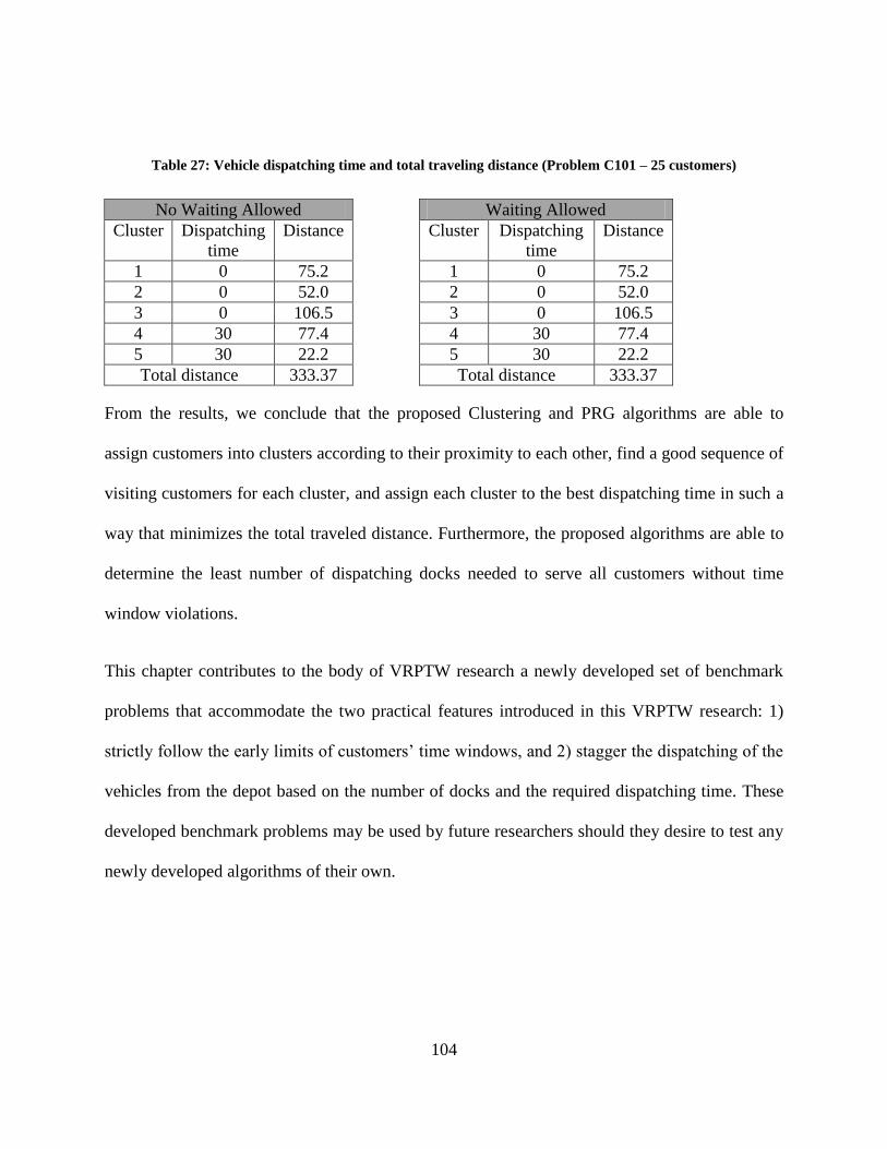
104
Table 27: Vehicle dispatching time and total traveling distance (Problem C101 – 25 customers)
No Waiting Allowed Waiting Allowed
Cluster Dispatching
time
Distance Cluster Dispatching
time
Distance
1 0 75.2 1 0 75.2
2 0 52.0 2 0 52.0
3 0 106.5 3 0 106.5
4 30 77.4 4 30 77.4
5 30 22.2 5 30 22.2
Total distance 333.37 Total distance 333.37
From the results, we conclude that the proposed Clustering and PRG algorithms are able to
assign customers into clusters according to their proximity to each other, find a good sequence of
visiting customers for each cluster, and assign each cluster to the best dispatching time in such a
way that minimizes the total traveled distance. Furthermore, the proposed algorithms are able to
determine the least number of dispatching docks needed to serve all customers without time
window violations.
This chapter contributes to the body of VRPTW research a newly developed set of benchmark
problems that accommodate the two practical features introduced in this VRPTW research: 1)
strictly follow the early limits of customers’ time windows, and 2) stagger the dispatching of the
vehicles from the depot based on the number of docks and the required dispatching time. These
developed benchmark problems may be used by future researchers should they desire to test any
newly developed algorithms of their own.
105
CHAPTER 6: RESEARCH SUMMARY AND FUTURE RESEARCH
DIRECTIONS
6.1 Research Summary
This research studied the VRPTW with additional features that often arise in practical situations
but are generally ignored in the theoretical VRPTW literature. The special features are:
1. Customers have strict time windows for receiving a vehicle, i.e., vehicles are not allowed
to arrive at the customer’s location earlier than the lower limit of the specified time
window
2. There is a limited number of loading/unloading docks for dispatching/receiving the
vehicles at the depot
The special features added new constraints to the VRPTW formulation that necessitated the
development of new efficient algorithms to deal with such constraints.
The proposed solution approach decomposed the problem into three stages: Clustering,
Scheduling, and Dispatching Time Assignment. Two novel algorithms are proposed for
clustering and routing, which along with the assignment algorithm work interdependently to
cluster customers into groups, generate the routes, and determine the best dispatching time from
the depot for each vehicle.
The developed Routing algorithm, named the Probabilistic Routing Generation (PRG) algorithm
was tested on a set of well-known TSPTW benchmark problems. The PRG algorithm reached the
106
best known solution for all tested benchmark problems. Next, the Clustering and the PRG
algorithms were tested on a set of well-known VRPTW benchmark problems. In most cases, the
outcome of the proposed algorithms was close to the best known solutions for these problems.
The deviation from the best-known solution depended on the tested problem instance.
We noted that, in their current structure, the benchmark problems cannot be used to
accommodate the two special features of the VRPTW of 1) strictly following the early limit of
time window, and 2) staggering the dispatching of the vehicles from the depot based on the
number of docks and the required dispatching time. The benchmark problems were slightly
modified using a documented systematic procedure, and the proposed Clustering, Routing, and
Assignment algorithms were implemented on the modified benchmark problems.
6.2 Research Contributions
The contributions of this research can be summarized as follow:
1. A new variant of VRPTW has been proposed and studied by adding two new features to
the original problem, these new features are:
a. Vehicles are not allowed to wait at customer’s premises in case of arrival before
the start of the desired time window.
b. Limited availability of loading docks at the depot
2. A new approach has been developed for solving the VRPTW problem that considers the
two additional constraints. The proposed approach simultaneously clusters customers,
routes vehicles, and assigns vehicles to dispatching times from the depot.
107
3. A new routing algorithm, the Probabilistic Routing Algorithm PRG, has been proposed
and developed to find the best sequence of visiting customers while satisfying the time
windows. The PRG algorithm can be applied alongside the clustering algorithm to solve
the VRPTW, or can be applied independently to solve the TSPTW.
4. A new clustering algorithm has been developed that divides customers into groups
according to their proximity from each other. The clustering algorithm works
concurrently with the PRG algorithm to develop clusters while considering the time
windows of the customers.
5. A new set of benchmark problems has been created by modifying several well-known
VRPTW benchmark problems. This new set of benchmark problems allows future testing
of any newly developed algorithms to solve the VRPTW when considering the two extra
features listed above.
6.3 Future Research Directions
The following areas are believed to be potential areas for further research:
1. Enhance the performance of the current Clustering algorithm by graphically modifying
the developed clusters to improve the obtained results and prevent cases in which the last
cluster is formed of geographically dispersed customers.
2. Study the parameters affecting the performance of the PRG algorithm to determine the
conditions under which the performance of the algorithm is at its best. This study will
also involve mining our solutions of the benchmark problems to investigate correlations
between PRG algorithm parameters and its performance.
108
3. Improve the computational speed of the clustering algorithm by redesigning the process
of customer assignment to clusters. Specifically, an unassigned customer is added to
cluster if and only if the early limit of the time window of customer is lower than the
departure time from the last customer in cluster x. This will improve the computational
efficiency of the clustering algorithm as it will reduce the number of iterations required to
find a customer that can fit within cluster x.
4. Develop a new heuristic inspired by the PRG algorithm for solving special cases in job
shop scheduling to determine the best sequence of processing jobs on single and multiple
machines. This may require us to modify the objective function and some of the
algorithm mechanics.
5. Apply the PRG algorithm to solve a special version of the Facility Layout Design
Problem, the Looped Layout Design Problem, in which we desire to determine the
allocation of manufacturing cells to locations around a loop so as to minimize the
congestion in the facility. Because of the computational efficiency of the PRG algorithm,
we will investigate the impact of designing the layout (or allocation) of the machines
around the loop so as to maximize the throughput capacity of a vehicle-based material
handling system. Each iteration of the PRG algorithm generates a layout for the machines
based on the frequency of assigning machines to positions around the loop in layouts
generated in previous iterations.
109
REFERENCES
Aarts, E., J. Korst, and W. Michiels, 2005, Simulated Annealing, Search Methodologies
Introductory Tutorials in Optimization and Decision Support Techniques p. 187-210.
Alvarengaa, G. B., G. R. Mateusb, and G. d. Tomic, 2007, A genetic and set partitioning two-
phase approach for the vehicle routing problem with time windows: Computers and
Operations Research, v. 34, p. 1561-1584.
Atkinson, J. B., 1994, A Greedy Look-ahead Heuristic for Combinatorial Optimization: An
Application to Vehicle Scheduling with Time Windows: The Journal of the Operational
Research Society, v. 45, p. 673-684.
Backer, B. D., and V. Furnon, 1997, Meta-heuristics in Constraint Programming Experiments
with Tabu Search on the Vehicle Routing Problem, 2nd International Conference on
Metaheuristics.
Backer, B. D., V. Furnon, P. Kilby, P. Prosser, and P. Shaw, 1997, Local Search in Constraint
Programming: Application to the Vehicle Routing Problem: Constraint Programming 97,
Proceedings of Workshop on Industrial Constraint-Directed Scheduling.
Balakrishnan, N., 1993, Simple Heuristics for the Vehicle Routeing Problem with Soft Time
Windows: The Journal of the Operational Research Society, v. 44, p. 279-287.
Benyahia, I., and J.-Y. Potvin, 1995, Generalization and Refinement of Route Construction
Heuristics using Genetic Algorithms: Proceedings of the 1995 IEEE International
Conference on Evolutionary Computation, p. 39–43.
Berger, J., M. Barkaoui, and O. Braysy, 2003, A Route-directed Hybrid Genetic Approach for
the Vehicle Routing Problem with Time Windows: Information Systems and Operations
Research v. 41, p. 179-194.
Berger, J., M. Salois, and R. Begin, 1998, A hybrid genetic algorithm for the vehicle routing
problem with time windows, Advances in Artificial Intelligence: Lecture Notes in
Computer Science, v. 1418/1998, Springer Berlin / Heidelberg.
Blanton, J. L., and R.L.Wainwright, 1993, Multiple Vehicle Routing with Time and Capacity
Constraints Using Genetic Algorithms: Proceedings of the Fifth International Conference
on Genetic Algorithms.
110
Blum, C., and A. Roli, 2003, Metaheuristics in Combinatorial Optimization: Overview and
Conceptual Comparison: ACM Computing Surveys, v. 35, p. 268-308.
Bräysy, O., 2003, A Reactive Variable Neighborhood Search for the Vehicle-Routing Problem
with Time Windows: INFORMS Journal on Computing, v. 15, p. 347-368.
Bräysy, O., W. Dullaert, and M. Gendreau, 2004, Evolutionary Algorithms for the Vehicle
Routing Problem with TimeWindows: Journal of Heuristics, v. 10, p. 587-611.
Bäck, T., and H.-P. Schwefel, 1993, An Overview of Evolutionary Algorithms for Parameter
Optimization: Evolutionary Computation, v. 1, p. 1-23.
Chenga, C.-B., and K.-P. Wangb, 2009, Solving a vehicle routing problem with time windows by
a decomposition technique and a genetic algorithm: Expert Systems with Applications, v.
36, p. 7758-7763.
Chiang, W.-C., and R. A. Russell, 1996, Simulated annealing metaheuristics for the vehicle
routing problem with time windows: Annals of Operations Research, v. 63, p. 3-27.
Christofides, N., and S. Eilon, 1969, An Algorithm for the Vehicle- dispatching Problem:
Operations Research, v. 20, p. 309-318.
Christofides, N., A. Mingozzi, and P. Toth, 1979, The vehicle routing problem: Chichester,
Wiley.
Christofides, N., A. Mingozzi, and P. Toth, 1981, Exact algorithms for the vehicle routing
problem, based on spanning tree and shortest path relaxation: Mathematical
Programming, v. 20, p. 255-282.
Clarke, G., and J. W. Wright, 1964, Scheduling of Vehicles from a Central Depot to a Number of
Delivery Points: Operations Research, v. 12, p. 568-581.
Cordeau, J.-F., G. Laporte, and A. Mercier, 2001, A Unified Tabu Search Heuristic for Vehicle
Routing Problems with Time Windows: The Journal of the Operational Research Society,
v. 52, p. 928-936.
Crainic, T. G., and G. Laporte, 1997, Planning models for freight transportation: European
Journal of Operational Research, v. 97, p. 409-438.
Czech, Z. J., and P. Czarnas, 2002, Parallel Simulated Annealing for the Vehicle Routing
Problem with Time Windows: 10th Euromicro Workshop on Parallel, Distributed and
Network-Based Processing.
111
Dantzig, G., R. Fulkerson, and S. Johnson, 1954, Solution of a Large-Scale Traveling-Salesman
Problem: Journal of Operations Research, v. 2, p. 393-410.
Debudaj-Grabysz, and Z. J. A. Czech, 2005, A Concurrent Implementation of Simulated
Annealing and Its Application to the VRPTW Optimization Problem KLUWER
International Series In Engineering And Computer Science, v. 777, p. 201-209.
Desrochers, M., J. Desrosiers, and M. Solomon, 1992, A New Optimization Algorithm for the
Vehicle Routing Problem with Time Windows Operations Research, v. 40, p. 342-354.
Desrochers, M., J. K. Lenstra, and M. W. P. Savelsbergh, 1990, A Classification Scheme for
Vehicle Routing and Scheduling Problems.: European Journal of Operational Research,
p. 322-332.
Dorigo, M., and G. D. Caro, 1999, The ant colony optimization meta-heuristic, New ideas in
optimization: Maidenhead, UK, McGraw-Hill Ltd.
Dorigo, M., and L. M. Gambardella, 1997, Ant Colony System: A Cooperative Learning
Approach to the Traveling Salesman Problem: IEEE Transactions on Evolutionary
Computation, v. 1, p. 53-66.
Dorigo, M., V. Maniezzo, and A. Colorni, 1996, The Ant System: Optimization by a colony of
cooperating agents: IEEE Transactions on Systems, Man, and Cybernetics-Part B, v. 26,
p. 29-41.
Dorigo, M., and T. Stützle, 2003, The Ant Colony Optimization Metaheuristic: Algorithms,
Applications, and Advances Handbook of Metaheuristics: International Series in
Operations Research & Management Science, v. 57: New York, Springer
Dumas, Y., J. Desrosiers, E. Gelinas, and M. Solomon, 1995, An optimal algorithm for the
traveling salesman problem with time windows: Operations Research, v. 43, p. 367-371.
Duych, R. J., 2008, Transportation Statistics Annual Report, Washington, DC, U.S. Department
of Transportation.
Fisher, M. L., and R. Jaikumar, 1981, A Generalized Assignment Heuristic for Vehicle Routing:
Networks, v. 11, p. 109-124.
Fleischer, M., 1995, Simulated Annealing: Past, Present, and Future, Winter Simulation
Conference.
Flood, M. R., 1956, The Traveling-Salesman Problem: Operations Research, v. 4, p. 61-75.
112
Gambardella, L. M., É. Taillard, and G. Agazzi, 1999, MACS-VRPTW: A Multiple Ant Colony
System for Vehicle Routing Problems with Time Windows, in M. D. a. F. G. D. Corne,
ed., New Ideas in Optimization: London, UK, McGraw-Hill, p. 63-76.
Garcia, B.-L., J.-Y. Potvin, and J.-M. Rousseau, 1994, A Parallel Implementation of the Tabu
Search Heuristic For Vehicle Routing Problems with Time Window Constraints:
Computers and Operations Research, v. 21, p. 1025-1033.
Gaskell, T. J., 1967, Bases for Vehicle Fleet Scheduling: Operational Research Society, v. 18, p.
281-295.
Gendreau, M., A. Hertz, and G. Laporte, 1992, New Insertion and Postoptimization Procedures
for the Traveling Salesman Problem: Operations Research, v. 40, p. 1086-1094.
Gillett, B. E., and L. R. Miller, 1974, A Heuristic Algorithm for the Vehicle-Dispatch Problem:
Operations Research, v. 22, p. 340-349.
Glover, F., 1986, Future paths for integer programming and links to artificial intelligence:
Computers and Operations Research, v. 13, p. 533-549.
Golden, B., and W. Stewart, 1991, Empirical Analysis of Heuristics, in J. K. L. E. L. Lawler, A.
H. G. Rinnooy Kan, D. B. Shmoys ed., The Traveling Salesman Problem: A Guided Tour
of Combinatorial Optimization: Chichester, John Wiley & Sons.
Golden, B. L., and E. A. Wasil, 1987, Computerized vehicle routing in the soft drink industry:
Operations Research, v. 35.
Gong, W., X. Liu, J. Zhang, and Z. Fu, 2007, Two-Generation Ant Colony System for Vehicle
Routing Problem with Time Windows: 2007 International Conference on Wireless
Communications Networking and Mobile Computing.
Halse, K., 1992, Modeling and solving complex vehicle routing problems, Technical University
of Denmark, Lyngby, Denmark.
Hansen, P., and N. Mladenovic, 2001, Variable neighborhood search: Principles and applications
European Journal of Operational Research, v. 130, p. 449-467.
Hertz, A., and D. Kobler, 2000, A framework for the description of evolutionary algorithms:
European Journal of Operational Research, v. 126, p. 1-12.
Hiquebran, D. T., A. S. Alfa, J. A. Shapiro, and D. H. Gittoes, 1993, A Revised Simulated
Annealing and Cluster-First Route-Second Algorithm Applied to The Vehicle Routing
Problem: Engineering Optimization, v. 22, p. 77-107.

113
Holland, J. H., 1975, Adaptation in Natural and Artificial Systems: Ann Arbor, University of
Michigan Press.
Ioannou, G., M. Kritikos, and G. Prastacos, 2001, A Greedy Look-Ahead Heuristic for the
Vehicle Routing Problem with Time Windows: The Journal of the Operational Research
Society, v. 52, p. 523-537.
Kirkpatrick, S., C. D. Gelatt, and M. P. Vecchi, 1983, Optimization by Simulated Annealing:
Science, v. 220, p. 671-680.
Kolen, A. W. J., A. H. G. R. Kan, and H. W. J. M. Trienekens, 1987, Vehicle Routing with Time
Windows: Operations Research, v. 35, p. 266-273.
Koskosidis, Y. A., W. B. Powell, and M. M. Solomon, 1992, An optimization-Based Heuristic
for Vehicle Routing and Scheduling with Soft Time Window Constraints: Transportation
Science, v. 26, p. 69-85.
Langevin, A., M. Desrochers, J. Desrosiers, S. Gélinas, and F. Soumis, 1993, A two-commodity
flow formulation for the traveling salesman and the makespan problems with time
windows: Networks, v. 23, p. 631–640.
Laporte, G., 2009, Fifty Years of Vehicle Routing: Transportation Science, v. 43, p. 408-416.
Lau, H. C., M. Sim, and K. M. Teo, 2003, Vehicle routing problem with time windows and a
limited number of vehicles: European Journal of Operational Research, v. 148, p. 559-
569.
Lenstra, J. K., and A. H. G. R. Kan, 1981, Complexity of vehicle routing and scheduling
problems: Networks, v. 11, p. 221-227.
Liberatore, F., G. Righini, and M. Salani, 2009, A Pricing Algorithm for the Vehicle Routing
Problem with Soft Time Windows, Innovations in Distribution Logistics, p. 251-266.
Little, J. D. C., K. G. Murty, D. W. Sweeney, and C. Karel, 1963, An Algorithm for the
Traveling Salesman Problem: Operations Research, v. 11, p. 972-989.
Liu, F.-H. F., and S.-Y. Shen, 1999a, A Route-Neighborhood-Based Metaheuristic for Vehicle
Routing Problem with Time Windows: European Journal of Operational Research, v.
118, p. 485-504.
Maffioli, F., 2003, The vehicle routing problem: A book review: Quarterly Journal of the
Belgian, French and Italian Operations Research Societies, p. 149-153.
114
Moreno-Vega, J. M., and a. B. Melián, 2008, Introduction to the special issue on variable
neighborhood search: Journal of Heuristics, v. 14, p. 403-404.
Nazif, H., and L. S. Lee, 2010, Optimized Crossover Genetic Algorithm for Vehicle Routing
Problem with Time Windows: American Journal of Applied Sciences, v. 7, p. 95-101.
Osman, I. H., 1993, Metastrategy simulated annealing and tabu search algorithms for the vehicle
routing problem Annals of Operations Research, v. 41, p. 421-451.
Osman, I. H., and G. Laporte, 1996, Metaheuristics: A bibliography: Annals of Operations
Research, v. 63, p. 511-623.
Paessens, H., 1988, The savings algorithm for the vehicle routing problem: European Journal of
Operational Research, v. 34, p. 336-344.
Pisinger, D., and S. Ropke, 2009, Large neighborhood search, in M. Gendreau, and J. Y. Potvin,
eds., Handbook of Metaheuristics.
Potvin, J.-Y., and S. Bengio, 1996, The Vehicle Routing Problem with Time Windows Part II:
Genetic Search: Informs Journal on Computing, v. 8, p. 165-172.
Potvin, J.-Y., D. Dubé, and C. Robillard, 1996, A Hybrid Approach to Vehicle Routing using
Neural Networks and Genetic Algorithms: Applied Intelligence, v. 6, p. 241-252.
Potvin, J.-Y., and J.-M. Rousseau, 1993, A parallel route building algorithm for the vehicle
routing and scheduling problem with time windows: European Journal of Operational
Research, v. 66, p. 331-340.
Prescott-Gagnon, E., G. Desaulniers, and L.-M. Rousseau, 2009, A Branch-and-Price-Based
Large Neighborhood Search Algorithm for the Vehicle Routing Problem with Time
Windows: Networks, v. 54, p. 190-204.
Qi, C., and Y. Sun, 2008, An Improved Ant Colony Algorithm for VRPTW: Proceedings of the
2008 International Conference on Computer Science and Software Engineering, p. 455-
458.
Russell, R. A., 1995, Hybrid Heuristics for the Vehicle Routing Problem with Time Windows:
Transportation Science, v. 29, p. 156-166.
Savelsbergh, M. W. P., 1985, Local search in routing problems with time windows: Local search
in routing problems with time windows, v. 4, p. 285-305.
Schulze, J., and T. Fahle, 1999, A parallel algorithm for the vehicle routing problem with time
window constraints: Annals of Operations Research, v. 86, p. 585-607.
115
Solomon, M. M., 1986, On the worst-case performance of some heuristics for the vehicle routing
and scheduling problem with time window constraints: Networks, v. 16, p. 161-174.
Solomon, M. M., 1987, Algorithms for the Vehicle Routing and Scheduling Problems with Time
Window Constraints: Operations Research, v. 35, p. 254-265.
Tan, K. C., L. H. Lee, Q. L. Zhu, and K. Ou, 2001a, Heuristic methods for vehicle routing
problem with time windows: Artificial Intelligence in Engineering, v. 15, p. 281-295.
Tan, K. C., L. H. Leeb, Q. L. Zhua, and K. Oua, 2001b, Heuristic methods for vehicle routing
problem with time windows: Artificial Intelligence in Engineering, v. 15, p. 281-295.
Tan, X., X. Zhuo, and J. Zhang, 2006, Ant Colony System for Optimizing Vehicle Routing
Problem with Time Windows (VRPTW), Computational Intelligence and Bioinformatics:
Lecture Notes in Computer Science, v. 4115: Berlin / Heidelberg, Springer
Thangiah, S. R., 1995a, Vehicle Routing with Time Windows Using Genetic Algorithms, in I. L.
Chambers, ed., Application Handbook of Genetic Algorithms:New Frontiers, v. II: Boca
Raton, CRC Press, p. 253-277.
Thangiah, S. R., 1995b, An Adaptive Clustering Method Using a Geometric Shape for Vehicle
Routing Problems with Time Windows: Proceedings of 6th International Conference on
Genetic Algorithms, p. 536–543.
Toth, P., and D. Vigo, 2002, The Vehicle Routing Problem: Discrete Mathematics and
Applications: Philadelphia, PA, USA, Society for Industrial and Applied Mathematics.
Voss, S., I. H. Osman, and C. Roucairol, 1999, Meta-Heuristics: Advances and Trends in Local
Search Paradigms for Optimization, Kluwer Academic Publishers Norwell, MA, USA.
Yellow, P. C., 1970, A Computational Modification to the Savings Method of Vehicle
Scheduling: Journal of the Operational Research Society, v. 21, p. 281-283.
Zhu, K. Q., 2000, A New Genetic Algorithm for VRPTW: IC-AI 2000.