SANDIA REPORT SAND2014-18782 Unlimited Release Printed October 2014

Multi-Target Camera Tracking, Hand-off and Display LDRD 158819 Final Report Robert J. Anderson Prepared by Sandia National Laboratories Albuquerque, New Mexico 87185 and Livermore, California 94550

Sandia National Laboratories is a multi-program laboratory managed and operated by Sandia Corporation, a wholly owned subsidiary of Lockheed Martin Corporation, for the U.S. Department of Energy's National Nuclear Security Administration under contract DE-AC04-94AL85000.

Approved for public release; further dissemination unlimited.

2

Issued by Sandia National Laboratories, operated for the United States Department of Energy by Sandia Corporation. NOTICE: This report was prepared as an account of work sponsored by an agency of the United States Government. Neither the United States Government, nor any agency thereof, nor any of their employees, nor any of their contractors, subcontractors, or their employees, make any warranty, express or implied, or assume any legal liability or responsibility for the accuracy, completeness, or usefulness of any information, apparatus, product, or process disclosed, or represent that its use would not infringe privately owned rights. Reference herein to any specific commercial product, process, or service by trade name, trademark, manufacturer, or otherwise, does not necessarily con-stitute or imply its endorsement, recommendation, or favoring by the United States Government, any agency thereof, or any of their contractors or subcontractors. The views and opinions expressed herein do not necessarily state or reflect those of the United States Government, any agency thereof, or any of their contractors. Printed in the United States of America. This report has been reproduced directly from the best available copy. Available to DOE and DOE contractors from U.S. Department of Energy Office of Scientific and Technical Information P.O. Box 62 Oak Ridge, TN 37831 Telephone: (865) 576-8401 Facsimile: (865) 576-5728 E-Mail: reports@adonis.osti.gov Online ordering: http://www.osti.gov/bridge Available to the public from U.S. Department of Commerce National Technical Information Service 5285 Port Royal Rd. Springfield, VA 22161 Telephone: (800) 553-6847 Facsimile: (703) 605-6900 E-Mail: orders@ntis.fedworld.gov Online order: http://www.ntis.gov/help/ordermethods.asp?loc=7-4-0#online

SAND 2014-18782 Unlimited Release

Printed October 2014

Multi-Target Camera Tracking,

Hand-off and Display LDRD

158819 Final Report

Robert J. Anderson Robotic & Security Systems Department

Sandia National Laboratories P.O. Box 5800

Albuquerque, New Mexico 87185-1125

Abstract

Modern security control rooms gather video and sensor feeds from tens to hundreds of cameras. Advanced camera analytics can detect motion from individual video streams and convert unexpected motion into alarms, but the interpretation of these alarms depends heavily upon human operators. Unfortunately, these operators can be overwhelmed when a large number of events happen simultaneously, or lulled into complacency due to frequent false alarms.

This LDRD project has focused on improving video surveillance based security systems by changing the fundamental focus from the cameras to the targets being tracked. If properly integrated, more cameras shouldn’t lead to more alarms, more monitors, more operators, and increased response latency but instead should lead to better information and more rapid response times. For the course of the LDRD we have been developing algorithms that takes live video imagery from multiple video cameras, identifies individual moving targets from the background imagery, and then displays the results in a single 3D interactive video. In this document we summarize the work in developing this multi-camera, multi-target system, including lessons learned, tools developed, technologies explored, and a description of currently capability.

4

Acknowledgement This work was funded under LDRD Project Number158819 and Title "Multi-Target Camera Tracking, Hand-off and Display". The author would like to thank Dan Small, John Wharton and Brad Parks for providing the motivation for investigating multiple target camera hand-off, and would like to thank team members Eric Gotlieb, Bryce Eldridge, Jon Whetzel, and Fred Rothganger for their support in developing this capability.

5

Contents 1.0 Introduction ............................................................................................................. 9

1.1 Evaluating the TLD (Tracking/Learning/Display) Algorithm. ................................. 9

1.2 Lessons Learned from 3D Video Motion Detection ............................................... 12

1.3 Fundamental Truisms in Camera Tracking ............................................................. 13

2.0 Hardware & Software. ................................................................................................ 15

2.1 Hardware ....................................................................................................... 15

2.2 Software Tools ....................................................................................................... 16

3.0 Algorithm Components ............................................................................................... 19

3.1 Camera Calibration from 3D Scans ........................................................................ 19

3.2 Image Reduction and Super Pixel Techniques ....................................................... 24

3.4 Metrics in Color Space............................................................................................ 30

3.5 Working with Extremal Sets ................................................................................... 34

3.6 Statistical Target Templates .................................................................................... 36

4.0 Building the Video Tracking System .......................................................................... 39

4.1 The Video Pipeline ................................................................................................. 39

4.2 The 3D MIRTH System .......................................................................................... 40

4.3 The 3D Display Subsystem. .................................................................................... 43

4.4 The Learning Subsystem and Overcoming the GIGO Problem ............................. 44

5.0 Conclusions ................................................................................................................. 48

6.0 Distribution: ................................................................................................................ 49

6

Figures Figure 1: TLD Algorithm tracking the author’s ear. 11 

Figure 2: Image from SAND2002-0801 Showing 3D VMD 12 

Figure 3: Indoor and Outdoor Axis IP Security Cameras with Varifocal lenses. 15 

Figure 4: Sample Unity Window Showing Scene Editor, Live Game Display, Scene Graph Hierarchy and Inspector. 17 

Figure 5: Scanning the Robot Vehicle Range with FARO scanner. 20 

Figure 6: Multiple scans combined for the RVR. 21 

Figure 7a: FARO Scan of Room Before Video Overlay, with Camera Calibration Tool 22 

Figure 7b. FARO Scan of Room with Full Video Overlay 22 

Figure 7c: Close up of Live Video Overlay 23 

Figure 8. Super pixel clustering of an image (small pixels, large pixels, restored image) 24 

Figure 9: Cycled Downsampling 25 

Figure 10a: Original Input Image 28 

Figure 10b: Four background copies of same image. 29 

Figure 11: Foreground Mask showing targets 29 

Figure 12: 2K color table used for indexed colors 32 

Figure 13: Original Input image and Restored image after Indexed Color 32 

Figure 14a Image difference with-out luminance scaling 33 

Figure 14b: Image difference with luminance scaling. 33 

Figure 15: Example of Rectangular ROIs 34 

Figure 16: Extremal Set 35 

Figure 17: Sample Target Boundaries using Extremal Sets . 35 

Figure 18a. Statistical Target Map Example 1 37 

Figure 18b: Statistical Target Map Example 2. 38 

Figure 19 The Per-Camera Video Pipeline 40 

Figure 20: MIRTH System Components 41 

Figure 21: Extremal Set Polyhedron Carving 42 

Figure 22: Tracking 3D Targets within the 3D Environment. 44 

Figure 23: Using a 3D site model to systematically classify site features. 46 

7

Nomenclature MIRTH Multiple Intruder Real-Time Tracking and Handoff (describes our current algorithm)

ExtremalSet Our technique for efficiently wrapping blobs of image data.

3D VMD 3D Video Motion Detection.

RVR Robot Vehicle Range, a test-site at Sandia.

GIGO Garbage In/Garbage Out

IP Internet Protocol, used for cameras that transmit imagery over Ethernet.

Axis A manufacturer of IP cameras.

POE Power-over-Ethernet.

Q1602,Q1604 Camera model numbers for Axis cameras.

CCD Charge-couple device. The chip technology behind IP cameras.

FARO A commercial company that provides laser scan based surveying equipment.

E57 An industry format for porting laser scan depth data.

Unity3D /Unity A commercial game engine for creating 3D worlds.

nVidia A manufacturer of video cards, i.e., GPUs, and developer of CUDA.

CUDA The parallel processing computing language developed by nVidia.

SIMD Single Instruction, Multiple Data. A parallel computing approach.

FPS Frames per Second, IP cameras typically run between 15 and 30 FPS.

MJPEG Motion-Picture Group format for sending video data.

H-264 Another standard compression format for transmitting video

FFMPEG An open-source project for all things video.

ROI Region-of-Interest

CPU Central-Processing-Unit, i.e., primary desktop computer as opposed to GPU.

GPU Graphical Processing Unit, i.e., the Video Card.

OpenCV An open-source computer vision library.

Matlab A commercial tool/language for mathematical computing.

CMake A software tool for cross-platform development of software.

BSD Berkeley Software Distribution, a copyright standard for distributing open software.

8

C,C#,C++ Computing languages.

TLD Tracking/Learning/Detection a software algorithm.

LK Lucas-Kanade, a popular technique for feature tracking.

BRIEF,SIFT,SURF,Censure Feature descriptors for targets in imagery.

HOG Histogram of Oriented Gradients, a technique for tracking visual contours.

K-Means A data clustering algorithm.

Epipolar The geometry of stereo vision.

RANSAC Random Sample Consensus. A technique for fitting data to a model.

ViBe Video Background Extraction, a published algorithm for detecting motion in video.

RGB,BGR Three channel color imagery with Red-Green-Blue pixels (or reversed order)

RGBA Four channel imagery with additional “Alpha” transparency channel.

RGB-D Three channel color imagery with additional fourth channel depth.

Alpha Used here to represent the level of transparency in image data.

2D Two-dimensional. Imagery from cameras comes is processed as a 2D array of pixels.

3D Three-dimensional. Implies a world of textures mapped onto polyhedral objects that can be viewed from any direction when viewed within a game engine such as Unity3D.

GUI Graphical User Interface. The user interface for modern software.

PTZ Pan-Tilt-Zoom.

sRGB An industry standard representation of color for monitors and printers.

CIE L*a*b* French International Commission representation for colors.

PNG Portable Network Graphics, a standard format for saving image data to files.

OBJ Alias Wavefront developed format for polyhedral data.

9

1.0 Introduction

Individual networked cameras provide rich streams of data for monitoring physical sites, but do not in themselves improve security response. If integrated poorly, excessive cameras can overload and burden operators, making rapid, informed decisions in dynamic environments difficult to achieve. This project has set out to improve this situation, by tracking targets with respect to a three-dimensional model of a site, combining multiple views of a single target into a one trace, and presenting the results to the operator using video-gaming interactive displays. By integrating multiple networked cameras into a single system and applying statistical background extraction, advanced tracking and learning methods in combination with game engine based visuals we are developing a much more intuitive and knowledge based means to interact with visual data.

It is hard to cover three years’ worth of research any single document. The software repository for the project, for instance, has over a thousand entries, and new techniques and test routines are constantly developed.1 In this final report I hope to highlight the most valuable contributions of the research and describe not only the successes and new tools that have been developed, but some of the short comings and lessons learned.

1.1 Evaluating the TLD Algorithm. During spring 2011, Zdenek Kalal2 released Open Source code3 for his Ph.D. thesis work TLD (Tracking-Learning-Detection, aka “Predator”) and created a sensation in the video tracking community. Dr. Kalal successfully demonstrated many of the core features needed for security based tracking systems, as follows:

No prior information needed for tracking – operator simply defines a Region-of-Interest (ROI) square around a target.

The approach works for any type of target: vehicles, bodies, faces, animals, etc. Robustly handles translation, smooth rotation, and large changes in zoom/field of view. Algorithm continuously adapts and improves the underlying target descriptor. Once a target is taught, the algorithm will reacquire the target whenever it returns to the

field of view.

Our initial efforts involved evaluating Dr. Kalal’s algorithm to determine its appropriateness for security facilities. The expectation was that we could adapt this algorithm to the size and scope of security operations.

1 For the record, code has been mostly stored in the repository at https://isrc-svn.sandia.gov/repos/RVRRobotics with the bulk of the most recent work under the UnityPlugins subdirectory.

2 http://info.ee.surrey.ac.uk/Personal/Z.Kalal/tld.html 3

http://techland.time.com/2011/04/07/revolutionary-object-tracking-video-software-released-as-open-source

10

Initial Assessment The TLD algorithm was originally implemented in Matlab, using a single black and white web camera with resolutions of 320x240 pixels, and could process video tracks at 20 frames per second and while tracking a single target. Our expectation was that the use of multi-threaded C code and Graphical Processing Unit (GPU) processing, i.e., computing on the video card, could substantially improve these numbers and allow multiple targets to be tracked on a commercial IP camera image that could have ten times as many pixels.

Unfortunately our expectations for greater speeds were misguided. The TLD algorithm was already using well optimized C code within the Matlab framework by incorporating “mex4” files from OpenCV libraries. Some of the core computational features such as the Lucas-Kanade5 tracker were already implemented within OpenCV with highly optimized code.

With the release of the Open Source version of TLD6,7 a number of open source researchers8 attempted to improve the core speed of the algorithm as well by converting the Matlab code to C. Despite multiple efforts, none of these of the developers were able to get performance that exceeded the original Matlab implementation. After three years of activity the discussion groups and most related efforts to extend TLD have essentially ceased.

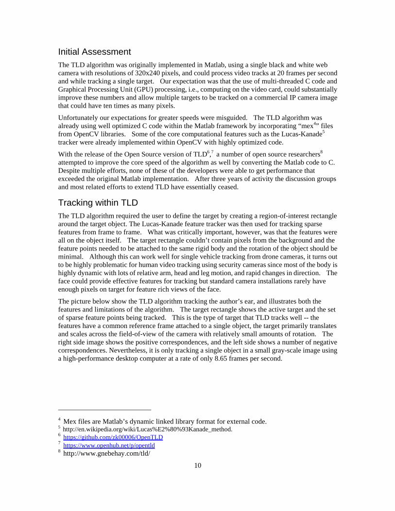
Tracking within TLD The TLD algorithm required the user to define the target by creating a region-of-interest rectangle around the target object. The Lucas-Kanade feature tracker was then used for tracking sparse features from frame to frame. What was critically important, however, was that the features were all on the object itself. The target rectangle couldn’t contain pixels from the background and the feature points needed to be attached to the same rigid body and the rotation of the object should be minimal. Although this can work well for single vehicle tracking from drone cameras, it turns out to be highly problematic for human video tracking using security cameras since most of the body is highly dynamic with lots of relative arm, head and leg motion, and rapid changes in direction. The face could provide effective features for tracking but standard camera installations rarely have enough pixels on target for feature rich views of the face.

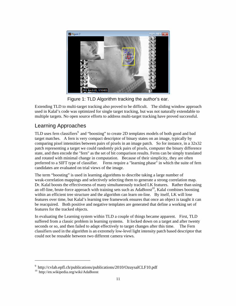
The picture below show the TLD algorithm tracking the author’s ear, and illustrates both the features and limitations of the algorithm. The target rectangle shows the active target and the set of sparse feature points being tracked. This is the type of target that TLD tracks well -- the features have a common reference frame attached to a single object, the target primarily translates and scales across the field-of-view of the camera with relatively small amounts of rotation. The right side image shows the positive correspondences, and the left side shows a number of negative correspondences. Nevertheless, it is only tracking a single object in a small gray-scale image using a high-performance desktop computer at a rate of only 8.65 frames per second.

4 Mex files are Matlab’s dynamic linked library format for external code. 5 http://en.wikipedia.org/wiki/Lucas%E2%80%93Kanade_method. 6 https://github.com/zk00006/OpenTLD 7 https://www.openhub.net/p/opentld 8 http://www.gnebehay.com/tld/

11

Figure 1: TLD Algorithm tracking the author’s ear.

Extending TLD to multi-target tracking also proved to be difficult. The sliding window approach used in Kalal’s code was optimized for single target tracking, but was not naturally extendable to multiple targets. No open source efforts to address multi-target tracking have proved successful.

Learning Approaches TLD uses fern classifiers9 and “boosting” to create 2D templates models of both good and bad target matches. A fern is very compact descriptor of binary states on an image, typically by comparing pixel intensities between pairs of pixels in an image patch. So for instance, in a 32x32 patch representing a target we could randomly pick pairs of pixels, computer the binary difference state, and then encode the "fern" as the set of bit comparison results. Ferns can be simply translated and rotated with minimal change in computation. Because of their simplicity, they are often preferred to a SIFT type of classifier. Ferns require a "learning phase" in which the suite of fern candidates are evaluated on trial views of the image.

The term “boosting” is used in learning algorithms to describe taking a large number of weak-correlation mappings and selectively selecting them to generate a strong correlation map. Dr. Kalal boosts the effectiveness of many simultaneously tracked LK features. Rather than using an off-line, brute-force approach with training sets such as AdaBoost10, Kalal combines boosting within an efficient tree structure and the algorithm can learn on-line. By itself, LK will lose features over time, but Kalal’s learning tree framework ensures that once an object is taught it can be reacquired. Both positive and negative templates are generated that define a working set of features for the tracked objects.

In evaluating the Learning system within TLD a couple of things became apparent. First, TLD suffered from a classic problem in learning systems. It locked down on a target and after twenty seconds or so, and then failed to adapt effectively to target changes after this time. The Fern classifiers used in the algorithm is an extremely low-level light intensity patch based descriptor that could not be reusable between two different camera views.

9 http://cvlab.epfl.ch/publications/publications/2010/OzuysalCLF10.pdf 10 http://en.wikipedia.org/wiki/AdaBoost

12

Moving Away From TLD Despite our initial enthusiasm for the approach, TLD did not provide the basis for multi-target, multi-camera security tracking that we had hoped for. The inability to extend it to multiple-targets, the requirements for user-based designation of targets, the inability to improve computing performance to enable extensions to mega-pixel color cameras, and the inability to hand-off fern-based target descriptors between cameras all proved too much to overcome. To achieve multiple-target tracking across multiple cameras we would have to develop a different approach.

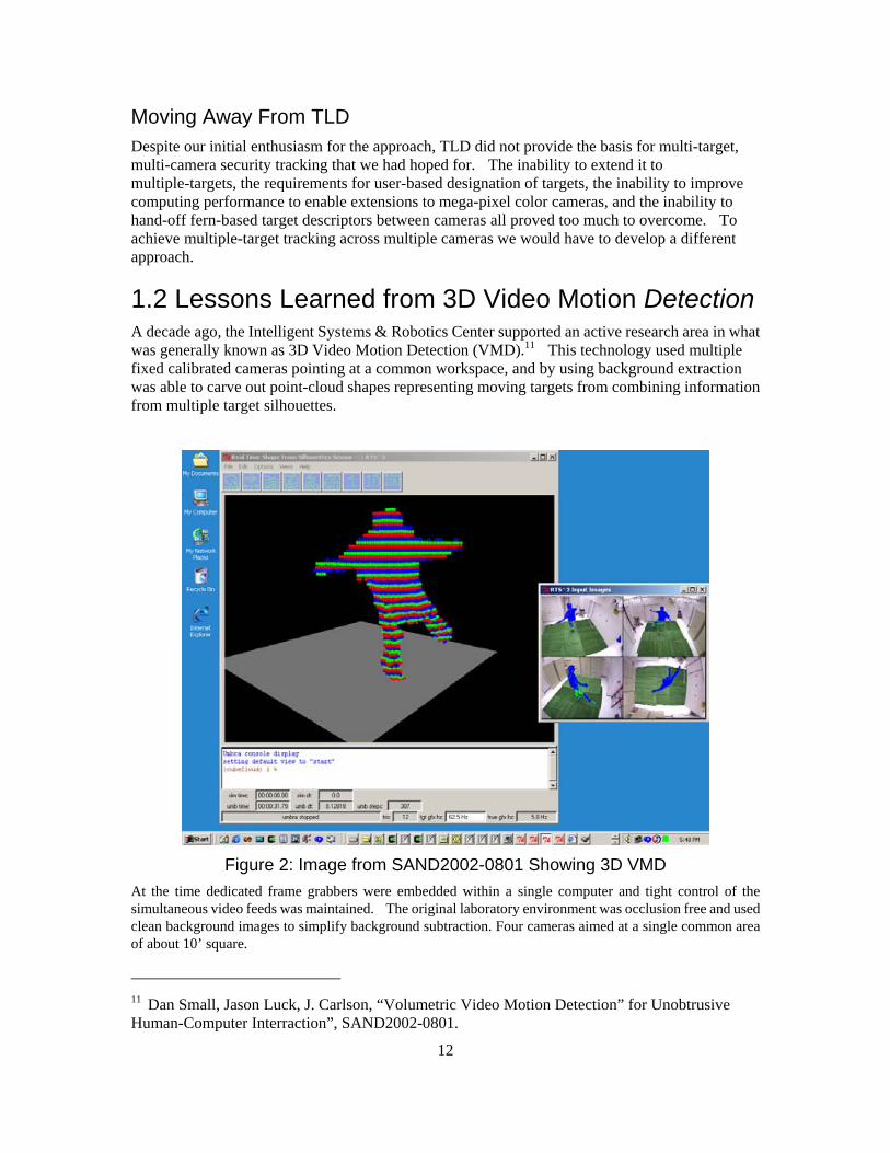
1.2 Lessons Learned from 3D Video Motion Detection A decade ago, the Intelligent Systems & Robotics Center supported an active research area in what was generally known as 3D Video Motion Detection (VMD).11 This technology used multiple fixed calibrated cameras pointing at a common workspace, and by using background extraction was able to carve out point-cloud shapes representing moving targets from combining information from multiple target silhouettes.

Figure 2: Image from SAND2002-0801 Showing 3D VMD

At the time dedicated frame grabbers were embedded within a single computer and tight control of the simultaneous video feeds was maintained. The original laboratory environment was occlusion free and used clean background images to simplify background subtraction. Four cameras aimed at a single common area of about 10’ square.

11 Dan Small, Jason Luck, J. Carlson, “Volumetric Video Motion Detection” for Unobtrusive Human-Computer Interraction”, SAND2002-0801.

13

After substantial success in the laboratory, this technology was applied to outdoor security systems, but ultimately failed to reach expectations. Because this LDRD is heavily invested in similar technology, i.e., the ability to track targets in a 3D space using fixed calibrated cameras it is important to understand why this technology fell short when applied to outdoor security applications.

From the outset, there are some clear barriers in implementing 3D-VMD for facility security. The re-quirements for overlapping intersecting volumes of multiple cameras would radically increase the number of cameras used to cover a facility. Current sites have one or possibly two cameras covering critical areas of a site. Furthermore, the reliance on a simple background differencing approach is likely to fail once outside the laboratory environment when lighting, background colors, and target occlusions are no longer controlled. Because a computer was needed to monitor each camera overlap area and required separate frame grabber cards with direct video connections for all overlapping cameras, the extension to a large area would result in an expensive mesh of interconnected video cables.

Ultimately, the difficulty in calibrating cameras was a major undoing of the 3D-VMD approach. Without accurate camera models the shape from silhouette approach couldn’t work, but obtaining accurate calibration for in-situ camera installations was not easily obtainable at the time. First cameras would have to be cali-brated in a laboratory cell for intrinsic parameters, and then have a secondary calibration for extrinsic pa-rameters at the site. If lens settings were ever changed, the entire process would have to be repeated.

Technology has advanced substantially in the last decade, and we will be taking advantage of two key ad-vancements: IP cameras, and RGB-D laser scanners. The IP cameras remove the video cable interconnect problem. Since a single IP camera can support multiple computer connections over Ethernet, there is no-longer a need for a complicated mesh of video cables to cover different overlap. In fact with Power over Ethernet (POE) cameras a single cable is used to plug in the camera and remotely power it. Because IP cameras can communicate over multiple sockets simultaneously, additional computers could be deployed to monitor different sectors without requiring any additional cabling.

Modern RGB-D scanners help overcome the camera calibration problem as will be described in section 3.1. By providing the background model containing both depth and color of a facility we will be able to calibrate the cameras in-situ directly from the model without any lab setups and without elaborate calibration fixtures.

1.3 Fundamental Truisms in Camera Tracking Before diving into the specifics of our multi-target tracking algorithms, we’d like to make explicit our working set of assumptions about the targets we plan on tracking. Each of these assertions then drives design decisions and focus areas.

You Can’t Be In Two Places At Once. This sounds obvious, but to take advantage of it we need to have precise video time synching and calibration. For fast moving targets, having low-latency video streaming (and highly synched video playback) is needed to allow triangulation of moving pixels. In practice we are able to keep our video streams within one frame (30msec) of each other.

A Leopard Can’t Change Its Spots. We plan on using texture features as the primary object to track, i.e., a distribution of color and edge features that moves with the target. Although clearly human target may pick-up objects and swap articles of clothing, the vast majority of image frames involve a target wearing the exact same set of clothes as in the previous frame.

Pigs Can't Fly. Nor for that matter, can pedestrians. Moving targets are assumed to be adjacent to the ground plane. This provides a lower bound on the target's position. From a 3D scan of a site, we can create a depth map for a camera, and determine the ground plane precisely. Single camera systems can be confused by things that do fly, like birds, moths, and the latest quad copter, but these are typically false alarm sources that can be eliminated with suitable camera overlap.

14

Shadows darken and lay flat. Shadows are problematic for video tracking. The shadow will confuse the camera's assessment of a moving target's feet, since the nearby shadow may extend well in front of the target's feet. To be less sensitive to this however, we can modify the pixel distance metric to be less sensitive to luminance variations. We can also reduce sensitivity by including “darkened” copies of current pixels in the background model. For really dark shadows, however, the best recourse may require a second camera and an epipolar pixel correspondence for potential shadow pixels that makes it clear they are being projected onto an existing surface.

An Object In Motion Tends to Stay In Motion. Targets that are being tracked can't suddenly jump across a room, nor immediately change their inertia. We can create a model of a targets motion, and use it to predict where they will be between frames.

Up is up. Thanks to gravity, objects have all kinds of vertical alignment. People’s bodies are over their feet. This also leads to many of targets having a certain level of axial symmetry. Video camera input should utilize that alignment.

Color constancy is a human delusion: Color perception is highly dependent on lighting. It changes throughout the day as the mixture of sunlight changes. Light incident angle and viewing angle can alter color perception. Camera BAYER (RGGB) cameras only detect and monitors only display a triangular subset of humans perceived color range. Cameras attempt to achieve white balance, but a largely "yellow room" such as our test lab can confuse them. Color calibration between cameras in different rooms needs to be able to take this into account.

15

2.0 Hardware & Software.

2.1 Hardware This project is focused on developing a video based security system for the immediate future and thus we focused our efforts on commercially available IP (Internet Protocol) cameras. We first evaluated a pair of Lumenera12 security cameras which had been approved for use for DOE security sites, but decided that they offered too less performance for the cost than some of the bigger IP camera manufacturers. We next evaluated cameras from Bosch, Basler, Sony, and AXIS and kept up to date on security camera testing being performed by an impartial video surveillance information website13. What we discovered in our early testing was that although the major vendors followed supposedly common protocols such as MJPEG and H.264, they didn’t all communicate seamlessly with the open source video library FFMPEG. The Axis cameras did however work with well with FFMPEG, and that combined with their affordable cost, their position as a market leader, and their excellent picture quality and product line resulted in our utilizing Axis camera products nearly exclusively for our research.

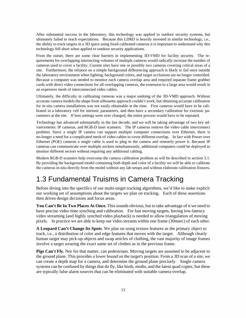
Figure 1 below shows indoor and outdoor versions of the Axis cameras. For the research we used a number of varieties of Axis cameras, including the models P1344, Q1602 and Q1604. The Q1602 offered better low-lux performance, while the Q1604 camera was a true Wide Dynamic Range (WDR) camera, which combines multiple exposure settings to prevent bright lights from saturating the entire image. All of the Axis cameras use a “varifocal” lens, which allows the user to adjust the focal length and focus of the lens over a small range, and then to tighten down the lens settings using thumbscrews. Fine focus is then performed digitally. All of the cameras are connected to the system using a single Power-over-Ethernet (POE) cable and configured from a web page. The camera web site also allows configuration of other parameters such as mask zones, audio recording, image size etc.

Figure 3: Indoor and Outdoor Axis IP Security Cameras with Varifocal lenses.

12 http://www.lumenera.com/ 13 http://ipvm.com/

16

2.2 Software Tools The goal of the research was to develop software systems that could provably track targets under real-world settings and provide a live demonstration capability that would show the algorithms at work. Thus software development was at the heart of the project. If a research approach couldn’t be feasibly implemented in real-time using a high-end desktop computer, then that approach wouldn’t be explored.

The general intention has been to be operating system agnostic. We have used CMake14 for building our source code and have used cross-platform tools that all work on Linux, Apple and Windows systems. In practice, the code has been primarily tested on Dell computers with CUDA supported NVIDIA GPUs15 running Windows 7 and compiled with Visual Studio 2010 and 2012.

OpenCV OpenCV is an open-source research library for computer vision under a BSD license.16 It has been around for twenty years, evolving from a C library to a pure C++ /CUDA library, but it has been over the last few years where the technology has really blossomed as GPU acceptance has become widespread. OpenCV provides a common image framework with minimal overhead that allows a wide variety of algorithms to be easily tested and compared. Camera calibration, feature detection, segmentation, feature matching, etc. have all been implemented within OpenCV, and as computer vision research evolves new algorithms are constantly being added to the repository. OpenCV wraps the FFMPEG library which in turn allows us to talk to a wide number of video capture sources including the H.264 video and MJPEG streams being generated by IP cameras. More importantly, the software library also provides a huge set of algorithms that have already been implemented within the CUDA framework that can otherwise plug-in with existing C-code.

We have used the OpenCV image framework (Mat) for all of our image work, and use their algorithms as a starting point for developing tracking algorithms. Because of the Open dynamic nature of the OpenCV we believe it does a good job of representing state-of-the-art implementations of computer vision algorithms. When a pre-coded routine exists within OpenCV we will test it and use it.

Unity3D Video imagery is fundamentally two dimensional, but it is viewing worlds that are three dimensional. This interplay between 2D projections and the 3D world is fundamental for 3D object tracking, and we need a method to visualize projections of 2D imagery in a 3D space. The Unity3D game engine17 provides a multi-platform engine18 the combines a scene graph, a highly optimized graphical display, a set of well documented software libraries, a 3D layout editor, and an ability to plugin external dynamic libraries, that provides all of the tools needed for 3D integration. Unity3D uses an innovative C# class mechanism for adding scripts to base class objects that makes it highly flexible for building applications.

14 www.cmake.org 15 https://developer.nvidia.com/cuda-gpus 16 http://en.wikipedia.org/wiki/BSD_licenses 17 www.unity3d.com 18 Runs on Windows, Apple, Linux, IPhones, tablets, consoles,

17

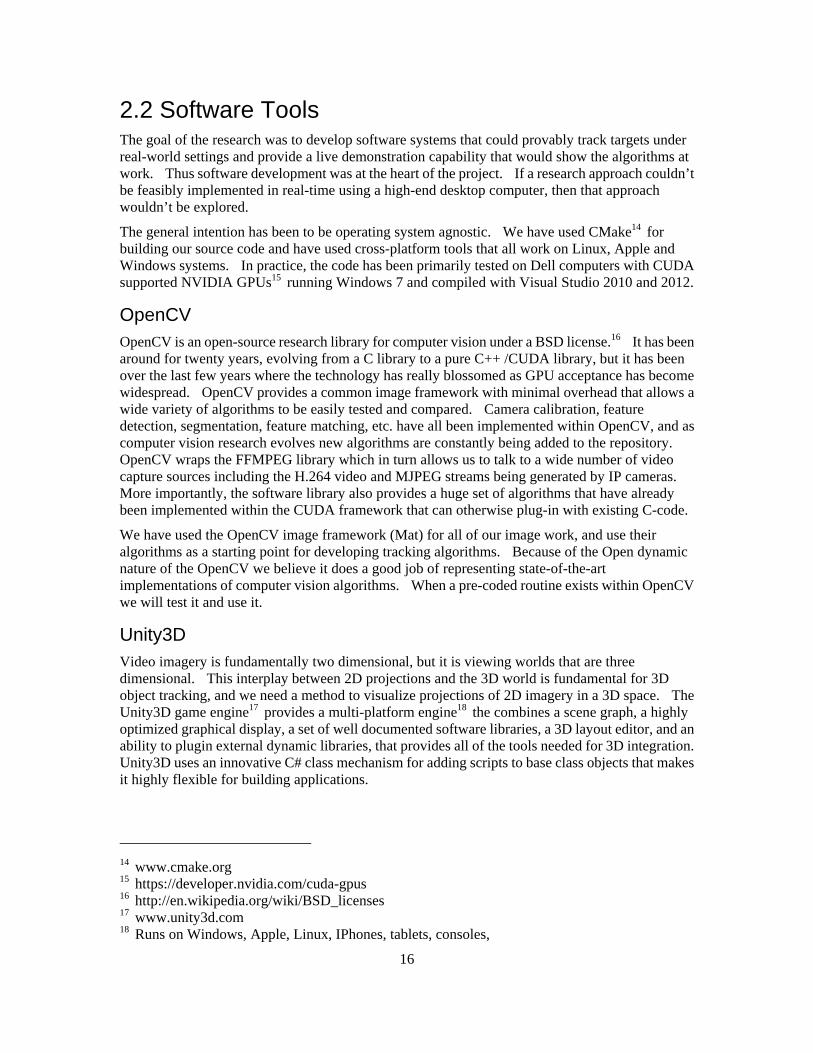
For our system, Unity3D is used for final system integration, operator user interfaces, camera calibration, and as a real-time diagnostic tool for code development. The vast majority of the heavy lifting in processing is done using attached dynamic libraries that use multi-threaded and GPU connections, but all of the spatially correlated information and dynamic displays are handled within the Unity Game environment.

Figure 4: Sample Unity Window Showing Scene Editor, Live Game Display, Scene Graph Hierarchy and Inspector.

CUDA19 CUDA (Compute Unified Device Architecture) is the proprietary computing language developed by NVidia to allow parallel programming to be implemented on NVidia video cards (i.e., Graphical Programming Units or GPUS). It has a C-like syntax and integrates seamlessly with CMake, and modern developer environments such as Visual Studio or Eclipse. Although it is more proprietary than OpenCL (which can also run on ATI video cards), it was the first general-computing solution for GPU programming and continues to have far greater user acceptance.

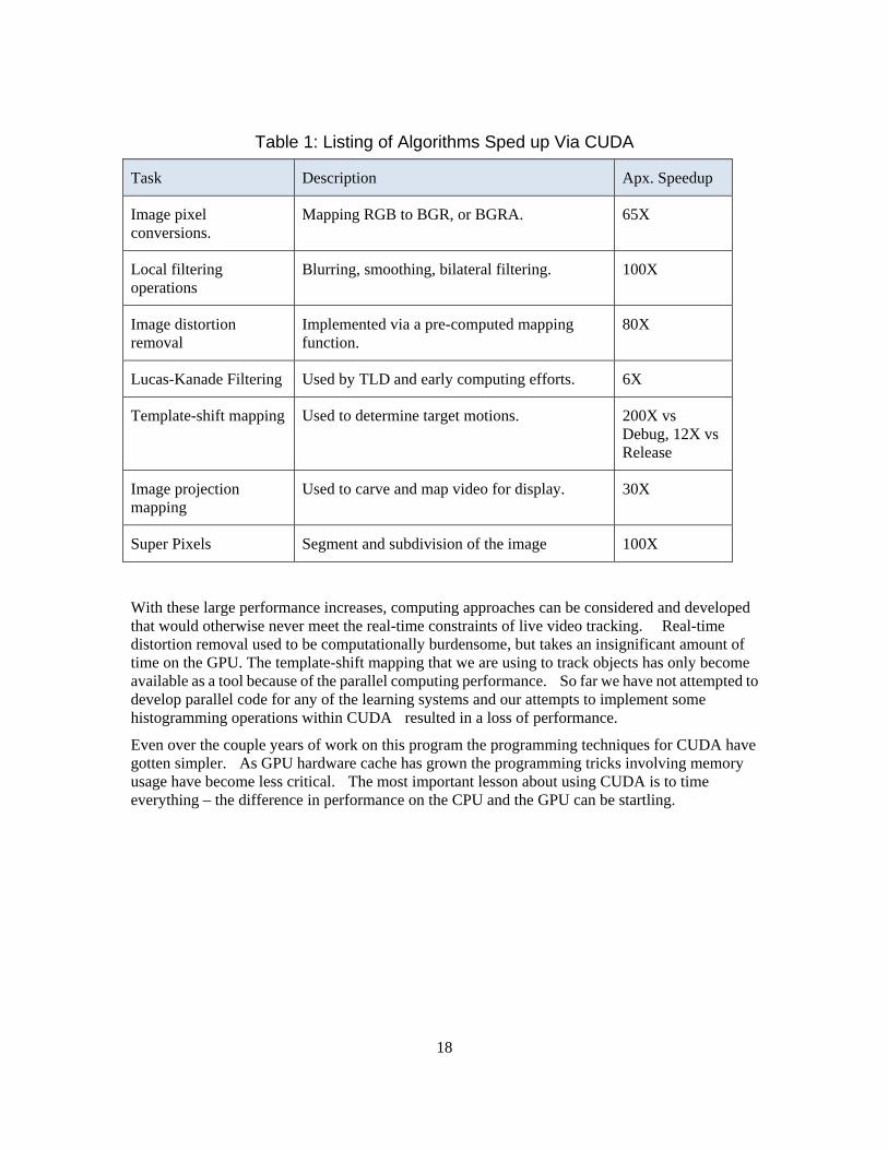
CUDA enables a number of operations to be performed in real-time that otherwise would not be possible for visual processing. CUDA enables SIMD programming, (single instruction, multiple data), where a single kernel of code is run simultaneously on multiple computing engines using different data sets Any video processing operation that can be applied to one patch within an image, and then duplicated with nearly the same code across the entire image are good candidates for CUDA implementation. For this class of operations we can see speed-ups of 100-fold compared to single threaded code running on the CPU. Tasks in the computing pipe-line that have been enhanced by running CUDA are listed in the table below.

19 http://www.nvidia.com/object/cuda_home_new.html

18

Table 1: Listing of Algorithms Sped up Via CUDA

Task Description Apx. Speedup

Image pixel conversions.

Mapping RGB to BGR, or BGRA. 65X

Local filtering operations

Blurring, smoothing, bilateral filtering. 100X

Image distortion removal

Implemented via a pre-computed mapping function.

80X

Lucas-Kanade Filtering Used by TLD and early computing efforts. 6X

Template-shift mapping Used to determine target motions. 200X vs Debug, 12X vs Release

Image projection mapping

Used to carve and map video for display. 30X

Super Pixels Segment and subdivision of the image 100X

With these large performance increases, computing approaches can be considered and developed that would otherwise never meet the real-time constraints of live video tracking. Real-time distortion removal used to be computationally burdensome, but takes an insignificant amount of time on the GPU. The template-shift mapping that we are using to track objects has only become available as a tool because of the parallel computing performance. So far we have not attempted to develop parallel code for any of the learning systems and our attempts to implement some histogramming operations within CUDA resulted in a loss of performance.

Even over the couple years of work on this program the programming techniques for CUDA have gotten simpler. As GPU hardware cache has grown the programming tricks involving memory usage have become less critical. The most important lesson about using CUDA is to time everything – the difference in performance on the CPU and the GPU can be startling.

19

3.0 Algorithm Components

A 3D video tracking system is a complex endeavor, with many components that need to work before the system is successful. The majority of the work done in the LDRD was involved in building these pieces. This section describes some of the more valuable components that have been developed.

3.1 Camera Calibration from 3D Scans Camera calibration is a critical component of any multi-target camera tracking system. One of the most fundamental truisms used in camera tracking is that you can’t be in two places at once. Where single camera systems ultimately give only two-dimensional information, multiple calibrated cameras viewing a common area pixels can be triangulated, and 3D information can be derived.

The Camera Model A modern security camera, such as the AXIS Q1602 consists of a varifocal lens coupled to a CMOS CCD imaging sensor, which in turn is locally processed with on-board camera electronics to produce a video stream to be sent over an Ethernet communication network typically using either a H.264 video protocol, or a MJPEG protocol. The camera may also provide video enhancements such as wide-dynamic-range, or motion stabilization, and will nearly always provide auto-iris control.

The video calibration process is the determination of the mapping between the camera pixels and rays in space. There is a long history of camera calibration in the literature, and we will use the conventional mathematical model20 with a few modifications in techniques. Whereas the conventional approach is to calibrate a camera in a laboratory setting using a known calibration fixture, this approach is not viable for most security settings in which the camera has already been deployed. In fact it was this difficulty in cali-brating cameras that contributed to the lack of acceptance of the 3D VMD system.

Typically camera calibration can be divided into two stages, intrinsic and extrinsic calibration. Intrinsic calibration involves the measurement of camera focal lengths, camera distortion, and pixel offsets. These characteristics are fundamental to a particular camera/lens combination and can be done off-line on a preci-sion bench top without a problem. For our intrinsic model we are using the model used within the OpenCV camera code21 but use only second and fourth order quadratic terms to represent distortion in the system. Once distortion parameters are estimated, image distortion can be reduced by running the image through an image distortion correction filter.

Using a Scanner to Aid Calibration Within OpenCV and Matlab, there is a process for calibrating cameras based off of taking a series of snap-shots from a checkerboard. There is no follow-up extrinsic calibration procedure, since their focus is on single camera systems, so the extrinsic frame is often attached to the camera. Our approach to calibrating

20 Zhang. A Flexible New Technique for Camera Calibration. IEEE Transactions on Pattern Analysis and Machine Intelligence, 22(11):1330-1334, 2000. 21 http://docs.opencv.org/modules/calib3d/doc/camera_calibration_and_3d_reconstruction.html

20

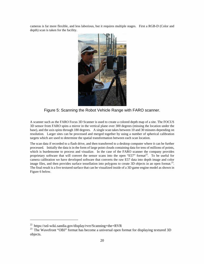
cameras is far more flexible, and less laborious, but it requires multiple stages. First a RGB-D (Color and depth) scan is taken for the facility.

Figure 5: Scanning the Robot Vehicle Range with FARO scanner.

A scanner such as the FARO Focus 3D Scanner is used to create a colored depth map of a site. The FOCUS 3D sensor from FARO spins a mirror in the vertical plane over 300 degrees (missing the location under the base), and the axis spins through 180 degrees. A single scan takes between 10 and 30 minutes depending on resolution. Larger sites can be processed and merged together by using a number of spherical calibration targets which are used to determine the spatial transformation between each scan location.

The scan data if recorded to a flash drive, and then transferred to a desktop computer where it can be further processed. Initially the data is in the form of large point clouds containing data for tens of millions of points, which is burdensome to process and visualize. In the case of the FARO scanner the company provides proprietary software that will convert the sensor scans into the open “E57” format22. To be useful for camera calibration we have developed software that converts the raw E57 data into depth image and color image files, and then provides surface tessellation into polygons to create 3D objects in an open format.23. The final result is a live textured surface that can be visualized inside of a 3D game engine model as shown in Figure 6 below.

22 https://snl-wiki.sandia.gov/display/rvrr/Scanning+the+RVR 23 The Wavefront “OBJ” format has become a universal open format for displaying textured 3D objects.

21

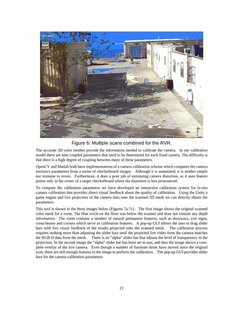
Figure 6: Multiple scans combined for the RVR.

The accurate 3D color meshes provide the information needed to calibrate the camera. In our calibration model there are nine coupled parameters that need to be determined for each fixed camera. The difficulty is that there is a high degree of coupling between many of these parameters.

OpenCV and Matlab both have implementations of a camera calibration scheme which computes the camera intrinsics parameters from a series of checkerboard images. Although it is automated, it is neither simple nor immune to errors. Furthermore, it does a poor job of estimating camera distortion, as it uses feature points only in the center of a target checkerboard where the distortion is less pronounced.

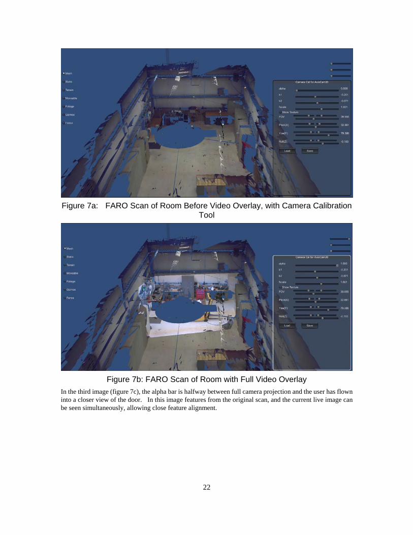
To compute the calibration parameters we have developed an interactive calibration system for in-situ camera calibration that provides direct visual feedback about the quality of calibration. Using the Unity a game engine and live projection of the camera data onto the scanned 3D mesh we can directly obtain the parameters.

This tool is shown in the three images below (Figures 7a-7c). The first image shows the original scanned color mesh for a room. The blue circle on the floor was below the scanner and does not contain any depth information. The room contains a number of natural permanent features, such as doorways, exit signs, cross-beams and corners which serve as calibration features. A pop-up GUI allows the user to drag slider bars with live visual feedback of the results projected onto the scanned mesh. The calibration process requires nothing more than adjusting the slider bars until the projected live video from the camera matches the RGB-D data from the mesh. There is an “alpha” slider bar that adjusts the level of transparency in the projection. In the second image the “alpha” slider bar has been set to one, and thus the image shows a com-plete overlay of the live camera. Even though a number of furniture items have moved since the original scan, there are still enough features in the image to perform the calibration. The pop-up GUI provides slider bars for the camera calibration parameters

22

Figure 7a: FARO Scan of Room Before Video Overlay, with Camera Calibration Tool

Figure 7b: FARO Scan of Room with Full Video Overlay

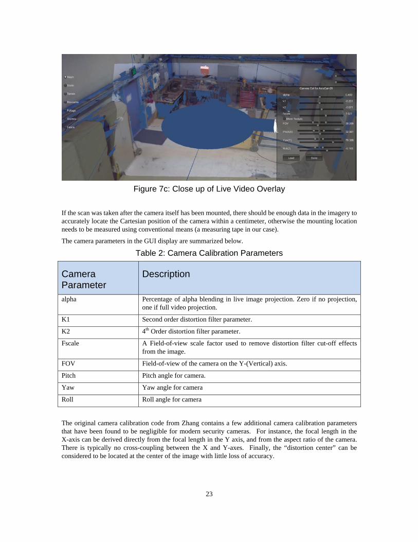
In the third image (figure 7c), the alpha bar is halfway between full camera projection and the user has flown into a closer view of the door. In this image features from the original scan, and the current live image can be seen simultaneously, allowing close feature alignment.

23

Figure 7c: Close up of Live Video Overlay

If the scan was taken after the camera itself has been mounted, there should be enough data in the imagery to accurately locate the Cartesian position of the camera within a centimeter, otherwise the mounting location needs to be measured using conventional means (a measuring tape in our case).

The camera parameters in the GUI display are summarized below.

Table 2: Camera Calibration Parameters

Camera Parameter

Description

alpha Percentage of alpha blending in live image projection. Zero if no projection, one if full video projection.

K1 Second order distortion filter parameter.

K2 4th Order distortion filter parameter.

Fscale A Field-of-view scale factor used to remove distortion filter cut-off effects from the image.

FOV Field-of-view of the camera on the Y-(Vertical) axis.

Pitch Pitch angle for camera.

Yaw Yaw angle for camera

Roll Roll angle for camera

The original camera calibration code from Zhang contains a few additional camera calibration parameters that have been found to be negligible for modern security cameras. For instance, the focal length in the X-axis can be derived directly from the focal length in the Y axis, and from the aspect ratio of the camera. There is typically no cross-coupling between the X and Y-axes. Finally, the “distortion center” can be considered to be located at the center of the image with little loss of accuracy.

24

3.2 Image Reduction and Super Pixel Techniques Modern IP cameras such as the Axis Q1604E can stream live images of 1280x720 pixels at 30 Frames per second (FPS), but live target tracking of multiple cameras at these image sizes can get bogged down, and most real-time image tracking approaches need to reduce the image sizes in order to maintain frame rates. The goal of the image reduction stage is to reduce the image size efficiently while maintaining information content. This balance between image size, efficiency and information has been constantly evolving throughout the LDRD.

Simplistic Downsizing The simplest way to reduce an image is to subsample the image. Take one pixel in a group, and throw out the rest. Clearly this will throw out a large amount of useful information, and could be achieved on the IP camera itself. Likewise, averaging all of the pixels in a window and returning the result is nearly as simple, can help reduce the impact of pixel noise, and can also performed directly on the camera before transmission, reducing network bandwidth.

The problem with these trivial approaches is that important edge and intensity information is lost and or distorted. Consider a reduced image of a checkerboard. If it is subsampled, the reduced image could contain all light pixels or all dark pixels and small position shifts would radically change the reduced image. In the averaged case, the pixels would come out gray and reflect neither color. The features of a target would change as its moves, since its edges are blended with different combinations of background.

The Super Pixel Approach Super pixels24 25 is a segmentation technique that maintains edge and color integrity in a region by applying K-Means clustering using a metric based on image distance and color distance. By iterating a few cycles on an image it is possible to divide an image into a much smaller set of like-colored regions. It is not an image size reduction technique per se, but can be when the shape information is ignored.

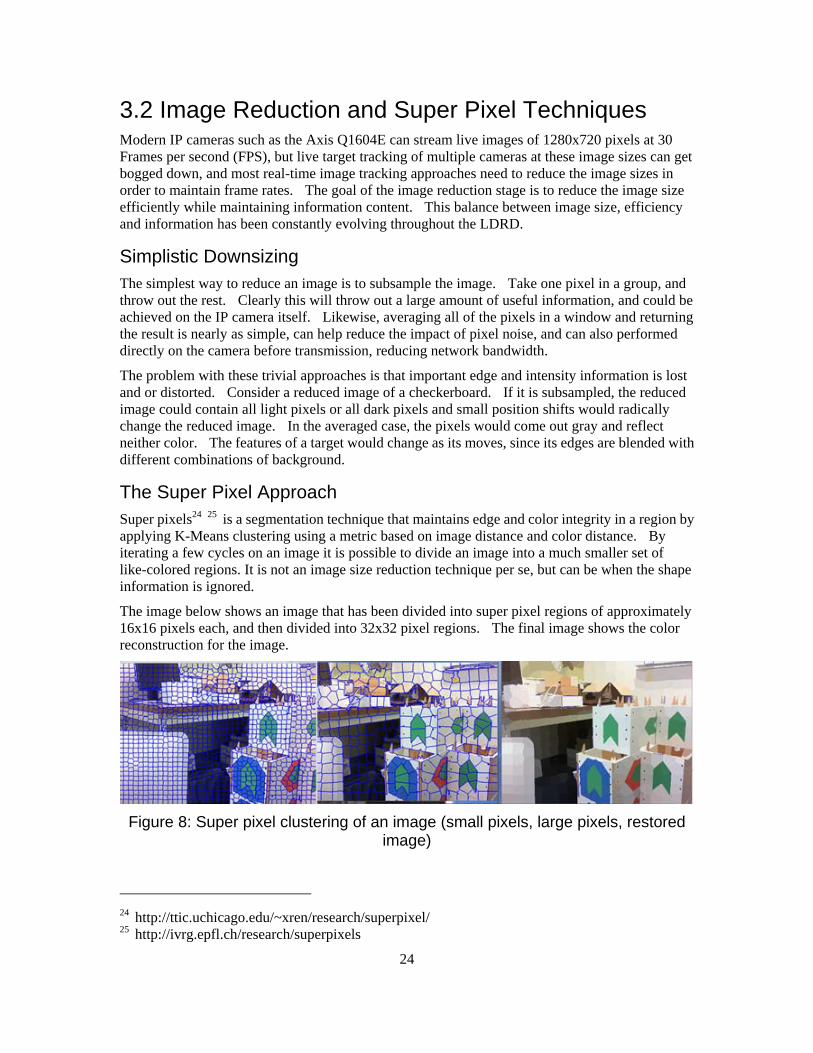
The image below shows an image that has been divided into super pixel regions of approximately 16x16 pixels each, and then divided into 32x32 pixel regions. The final image shows the color reconstruction for the image.

Figure 8: Super pixel clustering of an image (small pixels, large pixels, restored image)

24 http://ttic.uchicago.edu/~xren/research/superpixel/ 25 http://ivrg.epfl.ch/research/superpixels

25

The superpixel reduction can be performed in real-time but can still take 10 msec. to compute for a mega pixel image using a GPU. To recognize small targets we need still require smaller and smaller pixels sizes, so ultimately we started using 4x4 sized superpixels.

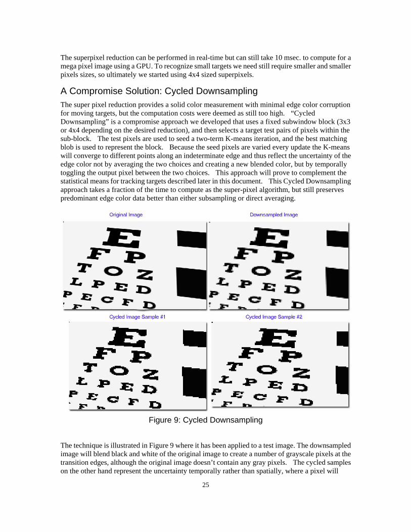
A Compromise Solution: Cycled Downsampling The super pixel reduction provides a solid color measurement with minimal edge color corruption for moving targets, but the computation costs were deemed as still too high. “Cycled Downsampling” is a compromise approach we developed that uses a fixed subwindow block (3x3 or 4x4 depending on the desired reduction), and then selects a target test pairs of pixels within the sub-block. The test pixels are used to seed a two-term K-means iteration, and the best matching blob is used to represent the block. Because the seed pixels are varied every update the K-means will converge to different points along an indeterminate edge and thus reflect the uncertainty of the edge color not by averaging the two choices and creating a new blended color, but by temporally toggling the output pixel between the two choices. This approach will prove to complement the statistical means for tracking targets described later in this document. This Cycled Downsampling approach takes a fraction of the time to compute as the super-pixel algorithm, but still preserves predominant edge color data better than either subsampling or direct averaging.

Figure 9: Cycled Downsampling

The technique is illustrated in Figure 9 where it has been applied to a test image. The downsampled image will blend black and white of the original image to create a number of grayscale pixels at the transition edges, although the original image doesn’t contain any gray pixels. The cycled samples on the other hand represent the uncertainty temporally rather than spatially, where a pixel will

26

converge to either the black or white solution and will toggle between them over time, as can be seen by comparing edges in two of the samples.

3.3 Background Subtraction Security installations tend to utilize fixed cameras for the majority of camera systems. Pan-tilt-zoom (PTZ) cameras may be used for better close-up evaluation of a target because they can put far more pixels on a target then even a 10 Mega-pixel camera can offer26, but they require an operator to use effectively, and can only monitor a single target at a time. PTZs are also more expensive, are prone to mechanical failures, and use far more power and space than fixed cameras. Most importantly, however, fixed cameras allow background subtraction techniques to be applied to automatically identify a possible target of interest.

In theory, background subtraction should be simple. Take an image of the background with no targets, and simply “subtract” the background snapshot from the current snapshot. Let, represent the 2-D image intensity of a gray scale image, and represent the 2-D intensity image of the background. A simple difference test would look for points where the image intensity exceeded a given threshold. The equation,

1 0

,

defines a binary mask, where image intensity points have been exceeded. This image mask would then be used to find moving targets by looking for clusters of pixels that have changed. Unfortunately this approach is extremely naïve, and doesn’t account for many of the problems that occur in a typical image. The table below summarizes some of the reasons why naïve background extraction fails.

Table 3: Problems to Overcome in Background Subtraction Algorithms

Reason Description

Noise Camera array sensors all have a certain amount of sensor noise and constantly change even for a static scene

Color Approximation

A color CCD array consists of individual blue, red and green detectors that can only approximate a color. Color is only matched when considering an array of pixels in a patch

Lighting Variations

Sunlight varies in both intensity and spectrum throughout the day. Clouds, haze, fog, etc. will all impact the color

Auto-Iris corrections

Most cameras use auto-iris adjustment, where the exposure level is adjusted to maintain a good average exposure level over the entire image. More sophisticated cameras may use some variation of Wide-Dynamic-Range

26 A 60 degree FOV PTZ 1 mega pixel camera with 10X zoom such as the 2 Mega-Pixel SONY FCBEH4300, can zoom down to a 3-degree FOV subwindow, providing the equivalent of 800 Mega-pixels coverage within a 60 degree field of –view.

27

control, often blending images taken from different exposure levels. In either case, dark or light objects will impact the exposure of their neighboring pixels

Dynamic Worlds Static objects can be picked up and moved. Chairs are relocated, doors are left open. Shadows will shorten and lengthen throughout the day

Foliage motion Trees and bushes will blow in the wind, causing large variations in neighboring pixels

Camera Mount Vibration

No camera mount is perfect, and large focal lengths will amplify even the smallest amount of vibration

Camouflaged Targets

A well camouflaged non-moving target simply won’t be seen, but a moving camouflaged target can be detected if the differences are aggregated over time and space

A good background subtraction algorithm needs to constantly update the background to reflect the current average state, as well as the expected variations in the current state.

Initial Evaluations and ViBE Early in the project we evaluated a number of background extraction techniques that are designed to accommodate the afore mentioned issues.27 28 These methods included a Mixture of Gaussians approach, a codebook approach, a support-vector-machine approach (SILK)29, and a statistical background update approach called ViBE (Video Background Extraction)30. Ultimately the ViBE approach proved to be the most effective. It was better able to retain long-standing targets without absorbing them into the background, was able to deal with small localized variations, and was able to meet the real-time requirements for the project.

Vibe maintains multiple sampled copies of the background image, where clear background pixels are randomly chosen and replaced.

27 http://experienceopencv.blogspot.com/2011/01/background-subtraction-and-models.html 28 https://sites.google.com/site/backgroundsubtraction/Home 29 Li Cheng, M. Gong, D. Schuurmans, and T. Caelli. Real-time Discriminative Background Subtraction. IEEE Trans. Image Processing, 20(5), 1401-1414, 2011 30 Barnich & Droogenbroeck, Transactions on Image Processing, June 2011.

28

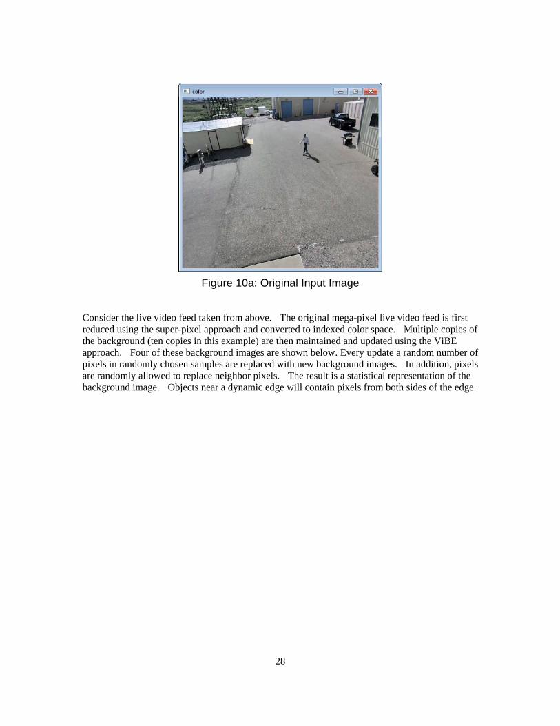
Figure 10a: Original Input Image

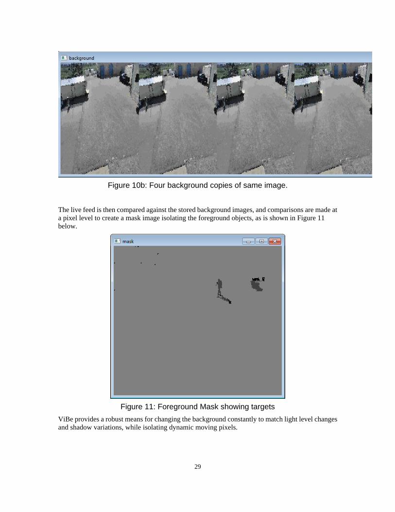
Consider the live video feed taken from above. The original mega-pixel live video feed is first reduced using the super-pixel approach and converted to indexed color space. Multiple copies of the background (ten copies in this example) are then maintained and updated using the ViBE approach. Four of these background images are shown below. Every update a random number of pixels in randomly chosen samples are replaced with new background images. In addition, pixels are randomly allowed to replace neighbor pixels. The result is a statistical representation of the background image. Objects near a dynamic edge will contain pixels from both sides of the edge.

29

Figure 10b: Four background copies of same image.

The live feed is then compared against the stored background images, and comparisons are made at a pixel level to create a mask image isolating the foreground objects, as is shown in Figure 11 below.

Figure 11: Foreground Mask showing targets

ViBe provides a robust means for changing the background constantly to match light level changes and shadow variations, while isolating dynamic moving pixels.

30

3.4 Metrics in Color Space The heart of all the background subtraction/color camera tracking is a metric. Historically many algorithms have used grayscale images, and the metric is simply the distance between illumination readings at a pixel. For color cameras, however, there is substantially more information available and the choice of an efficient metric for computing pixel differences is critical. Although CCD arrays are typically implemented as a Bayer pattern based array31 and consist of a repeating pattern of individual red, green and blue photosensors with twice as many green sensors as the red or blue components, the low level Bayer pattern is converted to a RGB image compressed and transmitted over Ethernet using either a MJPEG or H.264 protocol.

The FFMPEG decoder32 generates an array of color values in RGB space with a single 8bit character for each color channel resulting in a 256x256x256 levels of variation, or 16.7 Million distinct colors.

Color Spaces and Gamuts Strictly speaking the color output from the camera is considered to be sRGB33 color. This is the common denominator color used for internet imagery, monitor displays and printers and is the most common representation of color images. It is used by security camera vendors such as Axis since it displays directly on monitors without distorting the color. The sRGB space is a clipped color space, and highly saturated colors, especially greens, are clipped when represented in sRGB space. Other color spaces such as AdobeRGB or ProPhoto RGB have larger “gamuts “ , the represented subset of perceivable colors, but representing these colors with only a character per channel would give greater truncation between values.

The CIE L*a*b* color space is considered the gold standard of color spaces. The “L” stands for the luminance axis and maps directly to light intensity levels, while the a* and b* axes map to chrominance. It represents all perceptible colors, and distances between colors in this space are considered to be “perceptually uniform”, i.e., the Cartesian distance between points in this space can be used as a consistent metric of human perceptual difference across the range of colors.

From a computational point of view, however, CIE L*a*b* color space is problematic. The majority of the volume contained inside a CIE L*a*b* cube maps to no perceptible color, and less than 20% of the volume has a one-to-one mapping to sRGB space. The mapping between sRGB and CIE L*a*b* requires a series of computation steps.34

0.4124 0.3576 0.18050.2126 0.7152 0.07220.0193 0.1192 0.9502

31 http://en.wikipedia.org/wiki/Bayer_filter 32 We use OpenCV which in turn uses FFMPEG ( https://www.ffmpeg.org/) to decode video streams 33 http://en.wikipedia.org/wiki/Color_space 34 http://en.wikipedia.org/wiki/SRGB

31

/ 256 ∗ 12.92 10.35

256 0.055

1 0.055

.

otherwise

Where represents each color channel in the RGB image. The L*a*b* are then given by

∗ 116 16

∗ 500

∗ 200

Where

629

13296

429

And , , are the normalized white-point tristimulus values for the associated lighting which we set nominally to one. A similar set of equations for the inverse operations can be defined.

Computing this set of equations for every pixel during every image frame of a live video feed would slow the processing time to a crawl.

Creating a Metrically Indexed Color Space Euclidean distance in RGB space is simple to compute but is a poor metric, whereas CIE L*a*b* space provides the right distance metric but is unrealistic to compute in real-time. Our solution is to use an indexed color space, where each RGB color maps to an indexed color and the distance metrics for each index pair is pre-computed and stored in a table. This approach has a number of advantages. The image size if reduced from a three channel 24-bit image to a single channel 16 bit image. There is no longer any computation involved in computing the difference between two colors, just a table look-up between the two indices.

The size of the color table determines the minimum perceptible difference that needs to be recognized. A larger table represents more colors, but since the pre-computed distance table requires an NxN memory block there is a limitation in memory size. For our purposes a 2K size for the number of colors represented represents a reasonable compromise between color reproduction accuracy and memory table size.

The color table is created by creating a fixed grid within the CIE L*a*b*color space, and then keeping only those points which map to actual sRGB color values. Once the base color set is generated, a look-up table is computed which maps the original RGB color into indexed color

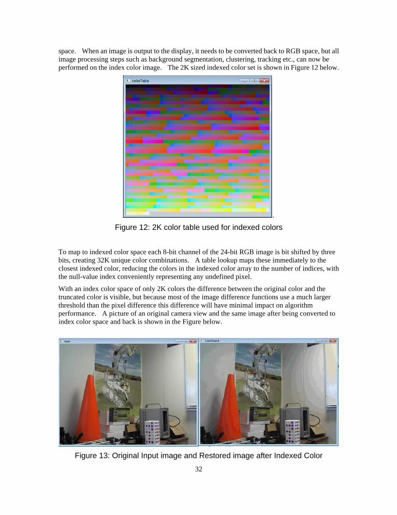
32

space. When an image is output to the display, it needs to be converted back to RGB space, but all image processing steps such as background segmentation, clustering, tracking etc., can now be performed on the index color image. The 2K sized indexed color set is shown in Figure 12 below.

.

Figure 12: 2K color table used for indexed colors

To map to indexed color space each 8-bit channel of the 24-bit RGB image is bit shifted by three bits, creating 32K unique color combinations. A table lookup maps these immediately to the closest indexed color, reducing the colors in the indexed color array to the number of indices, with the null-value index conveniently representing any undefined pixel.

With an index color space of only 2K colors the difference between the original color and the truncated color is visible, but because most of the image difference functions use a much larger threshold than the pixel difference this difference will have minimal impact on algorithm performance. A picture of an original camera view and the same image after being converted to index color space and back is shown in the Figure below.

Figure 13: Original Input image and Restored image after Indexed Color

33

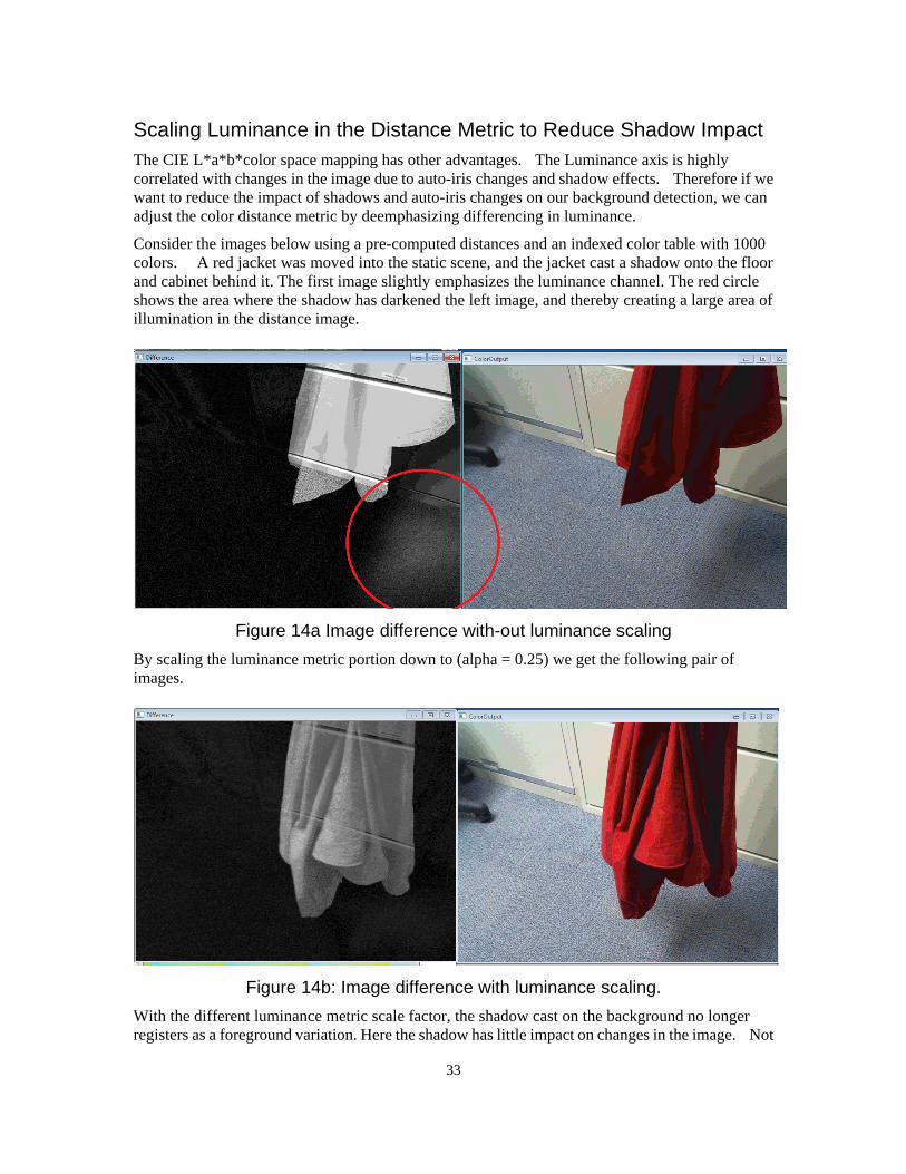
Scaling Luminance in the Distance Metric to Reduce Shadow Impact The CIE L*a*b*color space mapping has other advantages. The Luminance axis is highly correlated with changes in the image due to auto-iris changes and shadow effects. Therefore if we want to reduce the impact of shadows and auto-iris changes on our background detection, we can adjust the color distance metric by deemphasizing differencing in luminance.

Consider the images below using a pre-computed distances and an indexed color table with 1000 colors. A red jacket was moved into the static scene, and the jacket cast a shadow onto the floor and cabinet behind it. The first image slightly emphasizes the luminance channel. The red circle shows the area where the shadow has darkened the left image, and thereby creating a large area of illumination in the distance image.

Figure 14a Image difference with-out luminance scaling

By scaling the luminance metric portion down to (alpha = 0.25) we get the following pair of images.

Figure 14b: Image difference with luminance scaling.

With the different luminance metric scale factor, the shadow cast on the background no longer registers as a foreground variation. Here the shadow has little impact on changes in the image. Not

34

only does a reduced luminance metric help deemphasize shadows, but it also gives a reduced sensitivity to auto iris changes

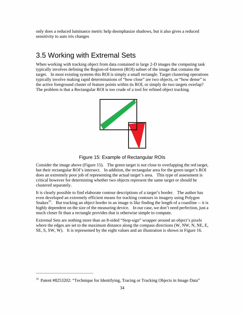
3.5 Working with Extremal Sets When working with tracking object from data contained in large 2-D images the computing task typically involves defining the Region-of-Interest (ROI) subset of the image that contains the target. In most existing systems this ROI is simply a small rectangle. Target clustering operations typically involve making rapid determinations of “how close” are two objects, or “how dense” is the active foreground cluster of feature points within its ROI, or simply do two targets overlap? The problem is that a Rectangular ROI is too crude of a tool for refined object tracking.

Figure 15: Example of Rectangular ROIs

Consider the image above (Figure 15). The green target is not close to overlapping the red target, but their rectangular ROI’s intersect. In addition, the rectangular area for the green target’s ROI does an extremely poor job of representing the actual target’s area. This type of assessment is critical however for determining whether two objects represent the same target or should be clustered separately.

It is clearly possible to find elaborate contour descriptions of a target’s border. The author has even developed an extremely efficient means for tracking contours in imagery using Polygon Snakes35. But tracking an object border in an image is like finding the length of a coastline -- it is highly dependent on the size of the measuring device. In our case, we don’t need perfection, just a much closer fit than a rectangle provides that is otherwise simple to compute.

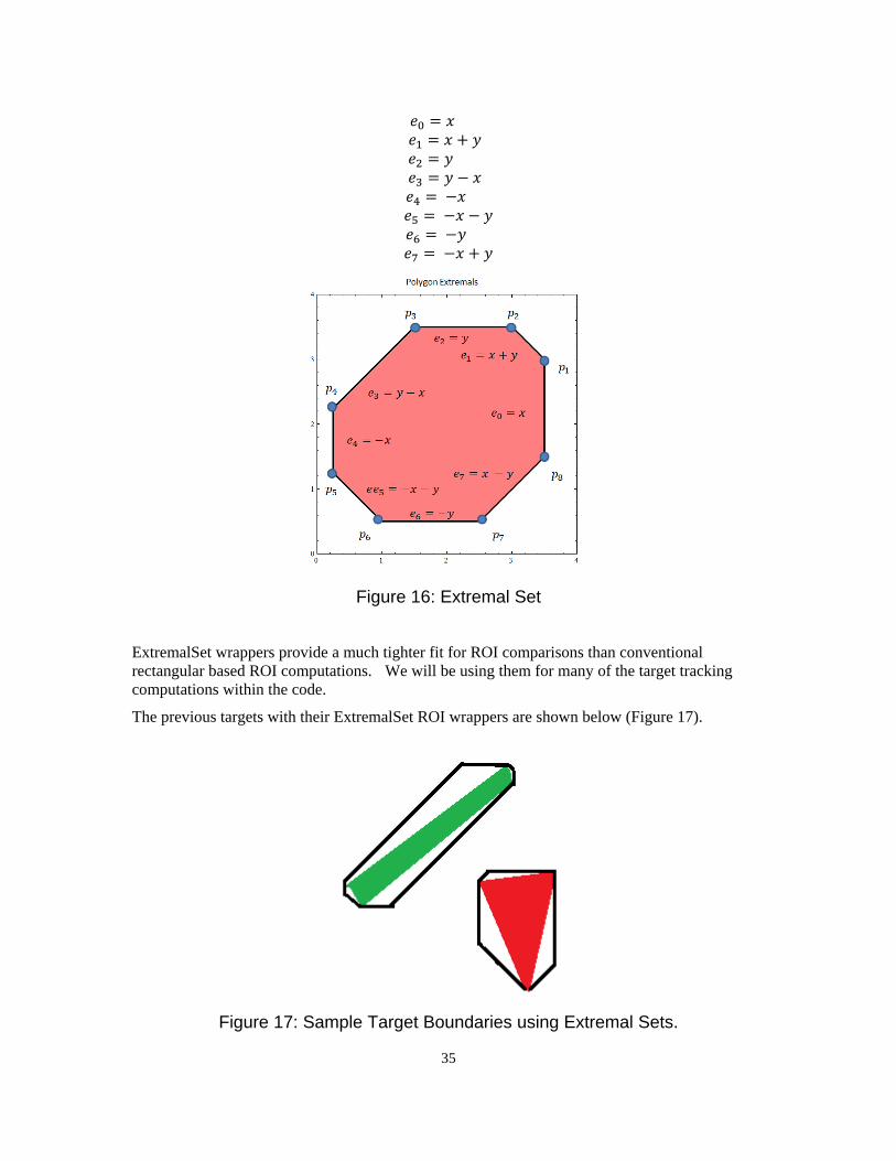
Extremal Sets are nothing more than an 8-sided “Stop-sign” wrapper around an object’s pixels where the edges are set to the maximum distance along the compass directions (W, NW, N, NE, E, SE, S, SW, W). It is represented by the eight values and an illustration is shown in Figure 16.

35 Patent #8253202: “Technique for Identifying, Tracing or Tracking Objects in Image Data”

35

Figure 16: Extremal Set

ExtremalSet wrappers provide a much tighter fit for ROI comparisons than conventional rectangular based ROI computations. We will be using them for many of the target tracking computations within the code.

The previous targets with their ExtremalSet ROI wrappers are shown below (Figure 17).

Figure 17: Sample Target Boundaries using Extremal Sets.

36

Computing the Area of the Extremal Set

The area of the extremal set can be computed from the vertices by summing up the cross products of each corner and dividing by half

If we expand this out for out special case, with we have

Simplifying we get the result as direct function of .

∗ 2

Similar rapid algorithms can be computed for perimeters, centroids, etc. To support image clustering operations we have developed a generic class for ExtremalSets that provides methods for computing area and centroids, finding gaps between other moving objects, computing unions and intersections and more. Extremal Sets represents a pragmatic compromise between crude rectangular ROIs and full polygonal contours of a surface.

3.6 Statistical Target Templates Our experience with TLD and OpenCV test libraries made it apparent that pixel-feature based trackers were inadequate for robust tracking of multiple targets in real-time. They performed too slowly for modern mega-pixel security cameras, and couldn’t handle large amounts of out-of-plane rotation, nor cover the large range in pixel resolution as a target moved. We experimented extensively with different feature detectors using different variations of “good features to track”, but the variability of moving human targets exceeded the ability of the detectors to track feature points. We also evaluated a number of other blob based tracking techniques available within the OpenCV framework, including the HOG (Histogram of Oriented Gradients) and the more generic “BlobTracker”. The Blob tracker could only perform at one frame per second on the live video feed, while the HOG filters performed poorly when target colors were too close to background colors.

The ViBE algorithm described in section 3.3 was designed to efficiently represent the statistical variation of the background by maintaining 10-20 copies of the background image and randomly replacing pixels in randomly chosen backgrounds with updated information. We decided to pursue a similar approach for tracking moving targets, but with a number of twists.

First, the target, by definition, is far more dynamic than the background. A target trace exists because it differs from the background, and it moves with respect to the background. The background is permanent, but the targets are fleeting. Therefore we would use far fewer image copies to represent each target (typically 3 or 4) to capture its shorter temporal content. Secondly, the goal of the research was to create a camera independent representation of the target that could be used by learning systems, thus the live capture of the target image would need to be remapped to

37

fixed template sizes. The size of the target in the image can change dramatically as a target moves from background to foreground, but the template size for the target should remain the same to allow algorithmic comparisons. Finally, the target was expected to be moving both rapidly and unpredictably, so rapid mechanisms that could compute the likely motion of the target needed to be computed in real-time.

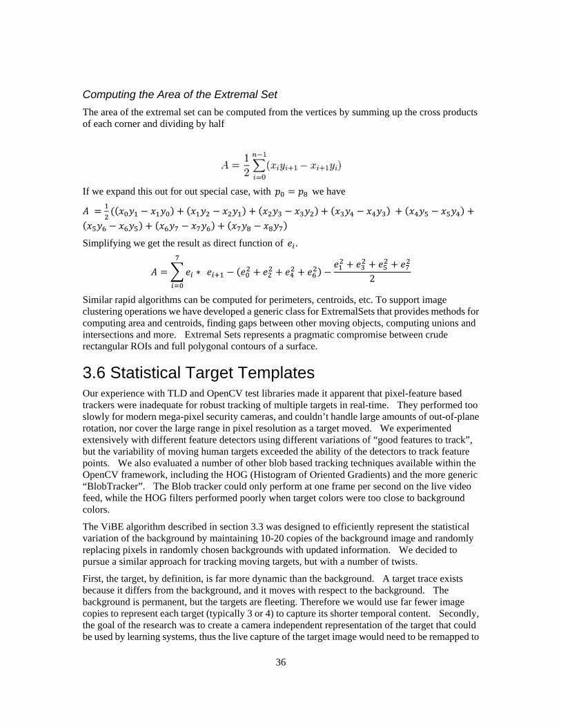
Consider Figures 18a and 18b below. Using clustering, region growing, and ExtremalSet based region definitions, two targets have been isolated. The right side of each image shows the templates that are being generated for both moving targets. Just as with the background extraction system, a subset of the pixels in the templates are randomly updated every image frame. In this system, three copies of each target are used to represent this short term temporal variance. Pixels that move rapidly, such as those corresponding to hands and feet tend to get blurred across the images, while the bulk of the pixels on the torsos are pretty consistent across the images. The template images are also a fixed size independent of the camera resolution or the location of the target in the foreground or background.

Figure 18a: Statistical Target Map Example 1

38

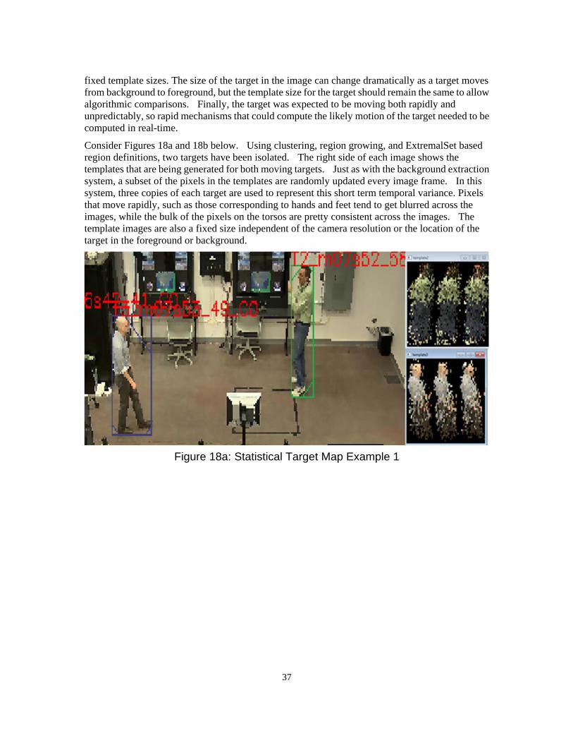
Figure 18b: Statistical Target Map Example 2.

Motion Tracking Using Statistical Targets Motion can be computed directly from the templates by using the power of brute-force GPU- based parallel programming and the simplicity of the indexed color model. During each update, the active template for a target is compared with the latest imagery. Using the GPU, the template can be shifted and scaled in parallel, and the number of pixel matches for each shift and scaling option can be computed on different simultaneous threads. A pixel is considered a match if the indexed color distance between it and one of the template copies is below a predefined threshold. The match metric is the just the total number of matching pixels between the latest frame and the template. The ROI motion can then be computed just by following the shifts and scaling factors that maximize this metric. The statistical target approach allowed us to find and track multiple targets in real-time, even though the targets moved were constantly occluded, turned rapidly, and often matched the background.

Learning from the Statistical Targets Templates The target templates that are generated for the motion tracking system also serve as the starting point for the learning system. When properly isolated, the templates represent the color distribution pattern of the moving target independent of the background. They can be further processed to create the “shirt-pants” descriptor, or the “totem-pole” descriptor described in section (4.3).

39

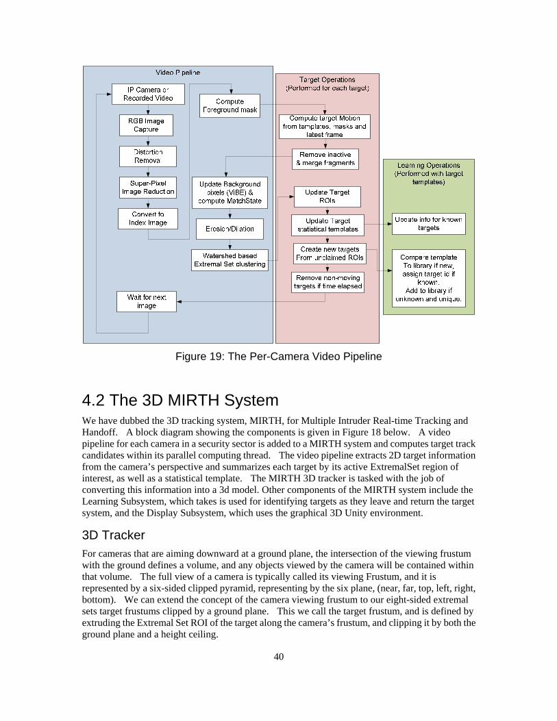
4.0 Building the Video Tracking System

This section describes how individual component technologies are combined to create a 3D Video tracking system.

4.1 The Video Pipeline The Video Pipeline processes each camera in the system on a separate CPU thread. With modern desktop computer systems there are typically multiple computer cores (4-16) available for processing, and the trend continues upward. By using threads it is possible to break up the computing task and process each pipeline on a separate core. Our target goal has been to process a minimum of four cameras on a single multi-core CPU, with future systems allowing eight or more. A large security site would devote rack-mounted computers to each multi-camera sector of a facility.

There are many stages in the video pipeline shown below (Figure 17). The primary pipeline process is fixed and works from the camera image to generate segmented indexed images. Distortion removal removes the barrel distortion from cameras with a wide field of view and insures that projective mapping will follow the pin-hole camera model in the 3D stages. The image is then taken through a super-pixel reduction process to reduce the image to a more manageable size without distorting the color information.

Once reduced, the RGB color image is converted to an index image. The background extraction technique would normally be performed next, but in order to improve the tracking of objects that match background images there is a tight interplay between the target tracking and the background image extraction. By using probability masks taken from the moving target templates, an assessment of how likely a given pixel matches the background or the target can be made. This prediction mask guides the background and foreground update process as it seeks to limit foreground target data from entering into the background model and background data entering into the moving target models.

Once a good estimate of foreground and background pixels has been computed, the clustering and segmentation operations can begin. Typically there is some noise in the process which can be eliminated via erosion and dilation techniques on the image. The clustering operations seek to find contiguous blobs of foreground points that can be treated as single entities.

Target operations proceed for any current active targets. The template shift algorithm is used to determine the latest motion for any active targets. Inactive targets are pruned, and target fragments that appear to be moving as a single object are merged. Any targets that have not moved at all for an extended period of time are absorbed into the background model.

Once the background mask is computed, clear foreground pixels are clustered. A watershed and clustering algorithm will then find target blobs that don’t correspond to any existing targets. If the target ROIs are suitably large this will lead to new target objects templates being created.

40

Figure 19: The Per-Camera Video Pipeline

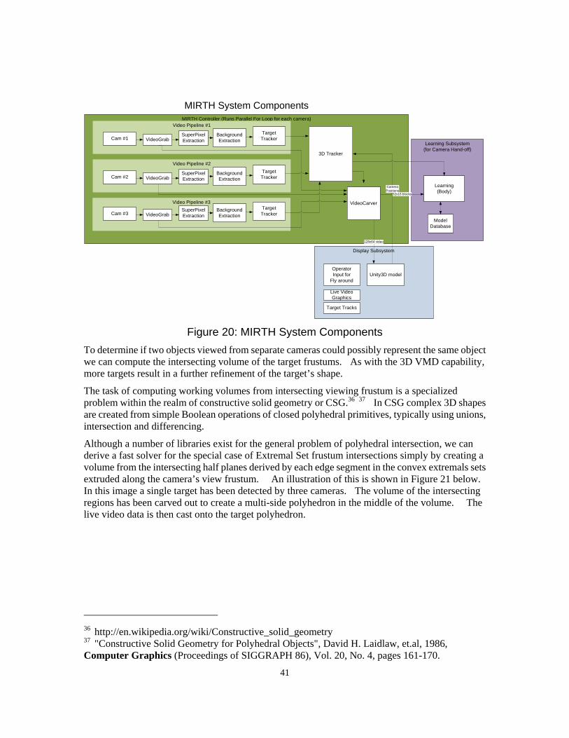
4.2 The 3D MIRTH System We have dubbed the 3D tracking system, MIRTH, for Multiple Intruder Real-time Tracking and Handoff. A block diagram showing the components is given in Figure 18 below. A video pipeline for each camera in a security sector is added to a MIRTH system and computes target track candidates within its parallel computing thread. The video pipeline extracts 2D target information from the camera’s perspective and summarizes each target by its active ExtremalSet region of interest, as well as a statistical template. The MIRTH 3D tracker is tasked with the job of converting this information into a 3d model. Other components of the MIRTH system include the Learning Subsystem, which takes is used for identifying targets as they leave and return the target system, and the Display Subsystem, which uses the graphical 3D Unity environment.

3D Tracker For cameras that are aiming downward at a ground plane, the intersection of the viewing frustum with the ground defines a volume, and any objects viewed by the camera will be contained within that volume. The full view of a camera is typically called its viewing Frustum, and it is represented by a six-sided clipped pyramid, representing by the six plane, (near, far, top, left, right, bottom). We can extend the concept of the camera viewing frustum to our eight-sided extremal sets target frustums clipped by a ground plane. This we call the target frustum, and is defined by extruding the Extremal Set ROI of the target along the camera’s frustum, and clipping it by both the ground plane and a height ceiling.

41

Display Subsystem

Learning Subsystem(for Camera Hand-off)

MIRTH Controller (Runs Parallel For Loop for each camera)Video Pipeline #1

ModelDatabase

MIRTH System Components

3D Tracker

VideoCarver

Unity3D model

Learning(Body)

128x64 video

Video Pipeline #2

VideoGrabSuperPixel Extraction

BackgroundExtraction

Target TrackerCam #1

Video Pipeline #3

VideoGrabSuperPixel Extraction

BackgroundExtraction

Target TrackerCam #2

VideoGrabSuperPixel Extraction

BackgroundExtraction

Target TrackerCam #3

CameraPositions

32x16 blocks

OperatorInput for

Fly around

Live VideoGraphics

Target Tracks

Figure 20: MIRTH System Components

To determine if two objects viewed from separate cameras could possibly represent the same object we can compute the intersecting volume of the target frustums. As with the 3D VMD capability, more targets result in a further refinement of the target’s shape.

The task of computing working volumes from intersecting viewing frustum is a specialized problem within the realm of constructive solid geometry or CSG.36 37 In CSG complex 3D shapes are created from simple Boolean operations of closed polyhedral primitives, typically using unions, intersection and differencing.

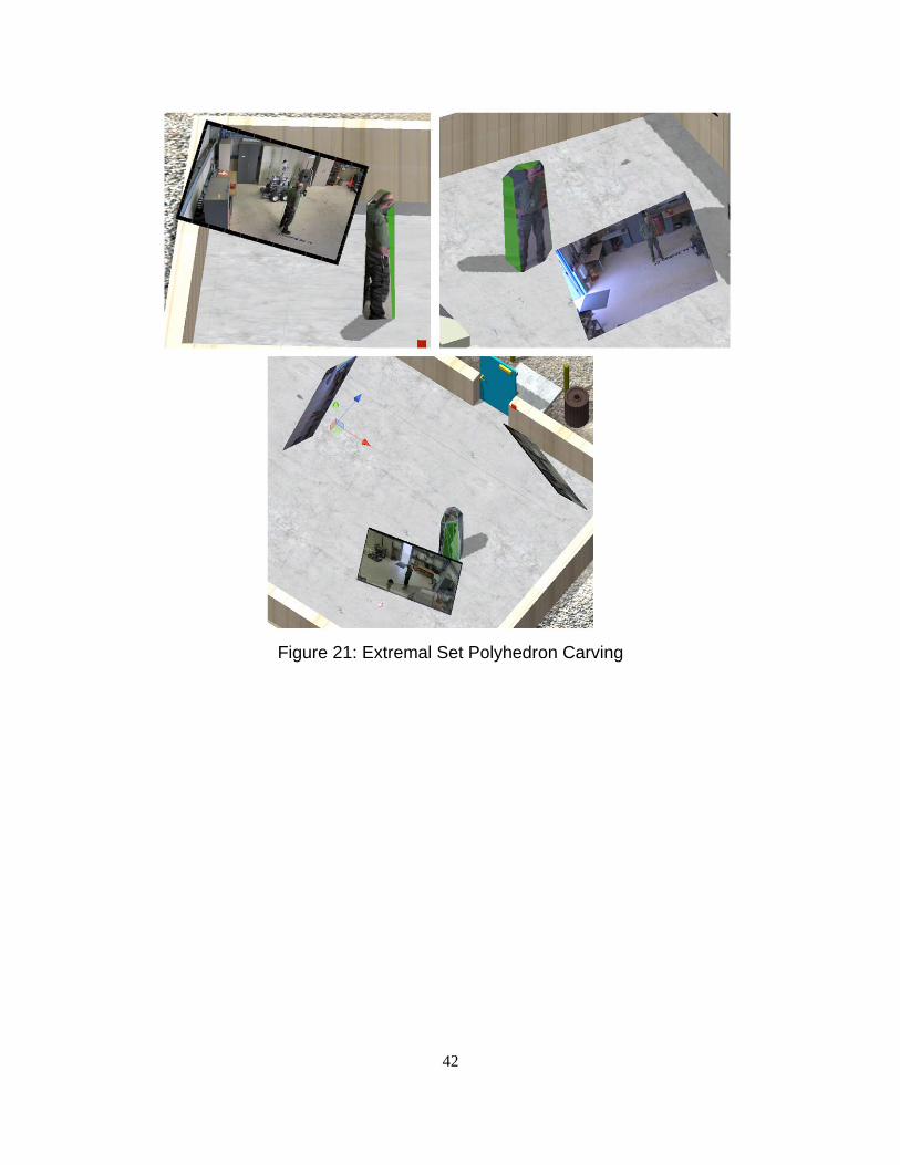
Although a number of libraries exist for the general problem of polyhedral intersection, we can derive a fast solver for the special case of Extremal Set frustum intersections simply by creating a volume from the intersecting half planes derived by each edge segment in the convex extremals sets extruded along the camera’s view frustum. An illustration of this is shown in Figure 21 below. In this image a single target has been detected by three cameras. The volume of the intersecting regions has been carved out to create a multi-side polyhedron in the middle of the volume. The live video data is then cast onto the target polyhedron.

36 http://en.wikipedia.org/wiki/Constructive_solid_geometry 37 "Constructive Solid Geometry for Polyhedral Objects", David H. Laidlaw, et.al, 1986, Computer Graphics (Proceedings of SIGGRAPH 86), Vol. 20, No. 4, pages 161-170.

42

Figure 21: Extremal Set Polyhedron Carving

43

4.3 The 3D Display SUBSYSTEM.

Conventional security display systems utilize a large panel of 2D images, representing the feeds from various security cameras. Imagery can be shown on separate monitors, or mapped to locations in a large video panel. Images can be locked to one camera, or switched between multiple live cameras. In all cases, however, the imagery is fundamentally two-dimensional and represented from the camera’s perspective. This approach creates a dilemma for site security system design – it makes it impossible to improve performance, while cutting costs.

The camera-centric paradigm for security systems is inherently self-limiting. More cameras detecting motion leads to more alarms, generate more video footage, require more operators to monitor the video feeds and will incur more costs. Operators need to understand the spatial location of each camera, i.e., building a mental map of the camera’s location with respect to a security sector, in order for them to order an effective response. Operator training time increases as cameras are added, and their stress levels increase with the rising complexity. If multiple cameras detect motion from the same target, this can result in a series of alarms, “lighting up” a security panel, and slowing effective response.

The multi-camera perspective promoted in this LDRD, however, works differently. Detected moving targets should generate individual alarms, irrespective of the number of cameras monitoring them. Adding more cameras to a sector should improve response performance, not degrade it. Once the infrastructure of POE gigabyte networks has been set-up, the cost of an individual camera is negligible38. It is the cost of monitor displays, operators and core infrastructure the drives security system costs.

The 3D display system we have developed uses a 3D model of a sector of interest. The 3D location of the target is determined by processing the target’s ROI frustum and using the camera’s calibration information. As target’s are identified, a pop-up display showing the best current imagery for that target is displayed, along with a pointer to the location of that target within the 3D model. The information is shown in real-time as it happens, and because it is embedded within a 3D world requires little training time for the operator to understand the location of the camera imagery with respect to the 3D site.

38 Our Axis cameras are $1K, but equivalent performing cameras such as the Cricket from Point Grey http://ww2.ptgrey.com/cricket are under $350.

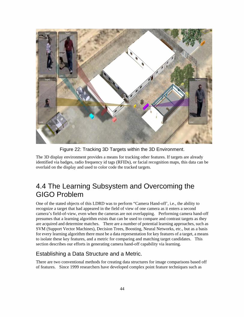
44

Figure 22: Tracking 3D Targets within the 3D Environment.

The 3D display environment provides a means for tracking other features. If targets are already identified via badges, radio frequency id tags (RFIDs), or facial recognition maps, this data can be overlaid on the display and used to color code the tracked targets.

4.4 The Learning Subsystem and Overcoming the GIGO Problem One of the stated objects of this LDRD was to perform “Camera Hand-off’, i.e., the ability to recognize a target that had appeared in the field of view of one camera as it enters a second camera’s field-of-view, even when the cameras are not overlapping. Performing camera hand-off presumes that a learning algorithm exists that can be used to compare and contrast targets as they are acquired and determine matches. There are a number of potential learning approaches, such as SVM (Support Vector Machines), Decision Trees, Boosting, Neural Networks, etc., but as a basis for every learning algorithm there must be a data representation for key features of a target, a means to isolate these key features, and a metric for comparing and matching target candidates. This section describes our efforts in generating camera hand-off capability via learning.

Establishing a Data Structure and a Metric. There are two conventional methods for creating data structures for image comparisons based off of features. Since 1999 researchers have developed complex point feature techniques such as

45

SIFT39 and SURF40 which generate a vector of floating point numbers (e.g., 128 numbers in an array) based off of image moments. These numbers describe the individual feature of interest and can be compared to other features by measuring the sum-of-square error distance of the features. Features of interest are locations in the image which have a measureable level of uniqueness, often centroids of intensity blobs, or corners. More recently a number of simpler fern like features detectors such as BRIEF 41 and CenSureE 42have become popular which uses bit wise comparisons at pixel points surrounding the feature point, but use a much simpler Hamming distance (bit-wise comparison difference) feature metric. Typically there is also some structure in the data that allows obvious outliers to be pruned, typically using a RANSAC method. For instance if all feature are known to be on a common plane, at a large distance from a perspective model, or attached to a rigid body then a mathematical model can be used to evaluate likely features and eliminate features that are inconsistent with the model.

Unfortunately, after extensive testing within the OpenCV libraries, none of these conventional feature detector based learning systems proved to be adequate for processing moving target data from our live video feeds. The approaches were not robust to the occlusion, out-of-plane rotation, perspective distortion, and range of scale needed for target tracking. They don’t take advantage of background extraction techniques, and fail to achieve real-time performance for mega-pixel cameras. Most of the good features to track occur at the edges of moving targets, but stay along the edge contour while the object pivots, rather than turning with the target.

Targets in our live video images are defined by clumps of pixels that both differ from the background and moving as a group across the image. We needed a metric that would map more closely to this. To be effective the metric should describe the target features, but not the background. It should be independent of the camera parameters and the location of the target within the field-of-view. It should be representable as an array of numbers so it can be used within a conventional learning algorithm.

It has been this goal of not just tracking targets, but tracking targets while generating learning data that has driven the algorithm development in this project.

Shirt-Pants Descriptor The first system that we attempted that met the real-time requirements was a “Shirt-Pants” descriptor with a Naive Bayes classifier.43 The descriptor simply divides a given target region into an upper half and lower half, uses K-means to compute the “best” color for both regions, and feeds these values into a learning system. Surprisingly this approach worked fairly well, but with many caveats. Primarily the targets needed to have a dominant upper torso color and bottom torso color that differed from other targets and was consistent from all directions. In addition, the targets needed to be moving in the open without foreground occlusion and at a reasonable distance from each other.

39 http://en.wikipedia.org/wiki/Scale-invariant_feature_transform 40 http://en.wikipedia.org/wiki/SURF 41 (BRIEF) Binary Robust Independent Elementary Features (http://www.cs.ubc.ca/~lowe/525/papers/calonder_eccv10.pdf) 42 http://link.springer.com/chapter/10.1007%2F978-3-540-88693-8_8#page-1 43 http://en.wikipedia.org/wiki/Naive_Bayes_classifier

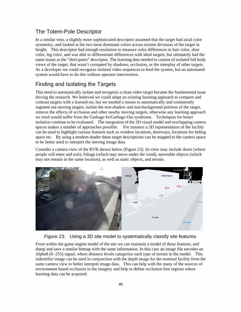
46

The Totem-Pole Descriptor In a similar vein, a slightly more sophisticated descriptor assumed that the target had axial color symmetry, and looked at the two most dominant colors across sixteen divisions of the target in height. This descriptor had enough resolution to measure color differences in hair color, shoe color, leg color, and was able to differentiate differences with ideal targets, but ultimately had the same issues as the “shirt-pants” descriptor. The learning data needed to consist of isolated full body views of the target, that wasn’t corrupted by shadows, occlusion, or the interplay of other targets. As a developer we could recognize isolated video sequences to feed the system, but an automated system would have to do this without operator intervention.

Finding and Isolating the Targets This need to automatically isolate and recognize a clean video target became the fundamental issue driving the research. We believed we could adapt an existing learning approach to compare and contrast targets with a learned set, but we needed a means to automatically and consistently segment out moving targets, isolate the non-shadow and non-background portions of the target, remove the effects of occlusion and other nearby moving targets, otherwise any learning approach we tried would suffer from the Garbage-In/Garbage-Out syndrome. Techniques for better isolation continue to be evaluated. The integration of the 3D visual model and overlapping camera spaces makes a number of approaches possible. For instance a 3D representation of the facility can be used to highlight various features such as window locations, doorways, locations for hiding space etc. By using a modern shader these target descriptions can be mapped to the camera space to be better used to interpret the moving image data.

Consider a camera view of the RVR shown below (Figure 23). Its view may include doors (where people will enter and exit), foliage (which may move under the wind), moveable objects (which may not remain in the same location), as well as static objects, and terrain.

Figure 23: Using a 3D site model to systematically classify site features.

From within the game engine model of the site we can maintain a model of these features, and dump and save a similar bitmap with the same information. In this case an image file encodes an Alpha8 (0.-255) signal, where distance levels categorize each type of terrain in the model. This indentifier image can be used in conjunction with the depth image for the nominal facility from the same camera view to better interpret image data. This can help with the many of the sources of environment based occlusion in the imagery and help to define occlusion free regions where learning data can be acquired.

47

Other techniques can also be pursued to improve learning data set acquisition. Shadows can be predicted and compensated for with more complex models that incorporate sun and light locations. When cameras overlap a workcell, epipolar constraint conditions can be used to define 3D correspondence at a pixel level. Hopefully these advanced approaches can be investigated within a future project.

48

5.0 Conclusions

This document has described the technology developed as part of a three-year LDRD project into video-based site security. By integrating multiple networked cameras into a single system and applying statistical background extraction, advanced tracking and learning methods we have developed an intuitive means to track and monitor targets within a facility. Numerous component technologies have been developed to support the work, including camera calibration from RGB-D scan data, high-speed image reduction using superpixels, precise and rapid image distance calculations using indexed color spaces, more precise region-of-interest tracking with ExtremalSets, and robust target tracking using statistical target templates.

All of these component technologies work together in the MIRTH (Multiple Intruder Real-Time Tracking & Hand-off) algorithm. MIRTH combines multi-core image pipe line processing with GPU-based processing to simultaneously process multiple live video feeds while computing the underlying locations in 3D. An integrated 3D model simplifies camera calibration and provides the framework for an interactive 3D operator console for the system. The result is a system that is target-centric -- not camera centric, reducing the cognitive burden for a security guard, while providing a pathway for integrating more cameras for even better performance.

Ultimately, we were not successful in implementing a functional camera-handoff capability. The target-template based descriptors looked promising as a first step in building a learning system for camera hand-off and preliminary learning descriptors did provide a level of target discrimination for distinct unoccluded targets. Extensions to more realistic targets however, require better processing of data in cluttered environments and further isolation of multiple overlapping targets for the learning process to be deployable. The 2D based target template descriptors themselves are probably too camera specific to be useful as a distinctive metric of the target to hand-off to another camera. Ultimately, a target descriptor needs to represent a large enough set of distinctive target features that even targets with similar clothing colors could be differentiated. This could be done by correlating pixels between two overlapping cameras using epipolar constraints and extracting information such as height and target width, but pursuing this approach requires greater resources than were available this project.

Indoor and outdoor functional demonstrations of the technology will remain at Sandia’s robot vehicle range and will evolve as this promising technology matures.

49

Distribution:

1 MS1125 Robert J. Anderson 6532

1 MS1125 Jake Deuel 6532

1 MS0762 Brad Parks 6630

1 MS9018 Central Technical File 8945-1

2 MS0899 Technical Library 9616

1 MS0612 Review & Approval Desk 9612

for DOE/OSTI