Single Target Tracking - pudn.comread.pudn.com/downloads91/sourcecode/book/348352/MATLAB Sim… · Single Target Tracking Tracking radar systems are used to measure the target™s

© 200

Chapter 9 Target Tracking

Single Target Tracking

Tracking radar systems are used to measure the target�s relative position inrange, azimuth angle, elevation angle, and velocity. Then, by using and keep-ing track of these measured parameters the radar can predict their future val-ues. Target tracking is important to military radars as well as to most civilianradars. In military radars, tracking is responsible for fire control and missileguidance; in fact, missile guidance is almost impossible without proper targettracking. Commercial radar systems, such as civilian airport traffic controlradars, may utilize tracking as a means of controlling incoming and departingairplanes.

Tracking techniques can be divided into range/velocity tracking and angletracking. It is also customary to distinguish between continuous single-targettracking radars and multi-target track-while-scan (TWS) radars. Trackingradars utilize pencil beam (very narrow) antenna patterns. It is for this reasonthat a separate search radar is needed to facilitate target acquisition by thetracker. Still, the tracking radar has to search the volume where the target�spresence is suspected. For this purpose, tracking radars use special search pat-terns, such as helical, T.V. raster, cluster, and spiral patterns, to name a few.

9.1. Angle TrackingAngle tracking is concerned with generating continuous measurements of

the target�s angular position in the azimuth and elevation coordinates. Theaccuracy of early generation angle tracking radars depended heavily on the

4 by Chapman & Hall/CRC CRC Press LLC

© 200

size of the pencil beam employed. Most modern radar systems achieve veryfine angular measurements by utilizing monopulse tracking techniques.

Tracking radars use the angular deviation from the antenna main axis of thetarget within the beam to generate an error signal. This deviation is normallymeasured from the antenna�s main axis. The resultant error signal describeshow much the target has deviated from the beam main axis. Then, the beamposition is continuously changed in an attempt to produce a zero error signal. Ifthe radar beam is normal to the target (maximum gain), then the target angularposition would be the same as that of the beam. In practice, this is rarely thecase.

In order to be able to quickly change the beam position, the error signalneeds to be a linear function of the deviation angle. It can be shown that thiscondition requires the beam�s axis to be squinted by some angle (squint angle)off the antenna�s main axis.

9.1.1. Sequential Lobing

Sequential lobing is one of the first tracking techniques that was utilized bythe early generation of radar systems. Sequential lobing is often referred to aslobe switching or sequential switching. It has a tracking accuracy that is lim-ited by the pencil beamwidth used and by the noise caused by either mechani-cal or electronic switching mechanisms. However, it is very simple toimplement. The pencil beam used in sequential lobing must be symmetrical(equal azimuth and elevation beamwidths).

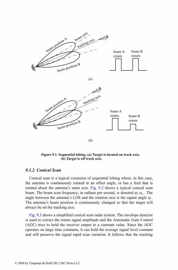
Tracking is achieved (in one coordinate) by continuously switching the pen-cil beam between two pre-determined symmetrical positions around theantenna�s Line of Sight (LOS) axis. Hence, the name sequential lobing isadopted. The LOS is called the radar tracking axis, as illustrated in Fig. 9.1.

As the beam is switched between the two positions, the radar measures thereturned signal levels. The difference between the two measured signal levelsis used to compute the angular error signal. For example, when the target istracked on the tracking axis, as the case in Fig. 9.1a, the voltage difference iszero. However, when the target is off the tracking axis, as in Fig. 9.1b, a non-zero error signal is produced. The sign of the voltage difference determines thedirection in which the antenna must be moved. Keep in mind, the goal here isto make the voltage difference be equal to zero.

In order to obtain the angular error in the orthogonal coordinate, two moreswitching positions are required for that coordinate. Thus, tracking in twocoordinates can be accomplished by using a cluster of four antennas (two foreach coordinate) or by a cluster of five antennas. In the latter case, the middleantenna is used to transmit, while the other four are used to receive.


© 200

9.1.2. Conical Scan

Conical scan is a logical extension of sequential lobing where, in this case,the antenna is continuously rotated at an offset angle, or has a feed that isrotated about the antenna�s main axis. Fig. 9.2 shows a typical conical scanbeam. The beam scan frequency, in radians per second, is denoted as . Theangle between the antenna�s LOS and the rotation axis is the squint angle .The antenna�s beam position is continuously changed so that the target willalways be on the tracking axis.

Fig. 9.3 shows a simplified conical scan radar system. The envelope detectoris used to extract the return signal amplitude and the Automatic Gain Control(AGC) tries to hold the receiver output to a constant value. Since the AGCoperates on large time constants, it can hold the average signal level constantand still preserve the signal rapid scan variation. It follows that the tracking

beam axis

tracking axis

beam positi

on A

beam position B

beam Areturn beam B

return

(a)

beam position B

beam positi

on Atracking axis

beam Areturn

beam Breturn

(b)

Figure 9.1. Sequential lobing. (a) Target is located on track axis. (b) Target is off track axis.

ωsϕ


© 200

error signals (azimuth and elevation) are functions of the target�s RCS; they arefunctions of its angular position off the main beam axis.

In order to illustrate how conical scan tracking is achieved, we will first con-sider the case shown in Fig. 9.4. In this case, as the antenna rotates around thetracking axis all target returns have the same amplitude (zero error signal).Thus, no further action is required.

tracking axis

beam axis

ϕ squint angle

rotatingfeed

Figure 9.2. Conical scan beam.

ωs

duplexertransmitter

mixer &IF Amp.

envelopedetector

AGCscan motor &scan reference

azimuth

detector error

elevation

detector error

Az & Elservo Amp servo motor

drive

Figure 9.3. Simplified conical scan radar system.


© 200

Next, consider the case depicted by Fig. 9.5. Here, when the beam is at posi-tion B, returns from the target will have maximum amplitude, and when theantenna is at position A, returns from the target have minimum amplitude.Between those two positions, the amplitude of the target returns will varybetween the maximum value at position B, and the minimum value at positionA. In other words, Amplitude Modulation (AM) exists on top of the returnedsignal. This AM envelope corresponds to the relative position of the targetwithin the beam. Thus, the extracted AM envelope can be used to derive aservo-control system in order to position the target on the tracking axis.

Now, let us derive the error signal expression that is used to drive the servo-control system. Consider the top view of the beam axis location shown in Fig.9.6. Assume that is the starting beam position. The locations for maxi-mum and minimum target returns are also identified. The quantity definesthe distance between the target location and the antenna�s tracking axis. It fol-lows that the azimuth and elevation errors are, respectively, given by

(9.1)

(9.2)

These are the error signals that the radar uses to align the tracking axis on thetarget.

beam axis

tracking axis

beam position A

beam position B

time

E t( )

E0

Figure 9.4. Error signal produced when the target is on the tracking axis for conical scan.

t 0=ε

εa ε ϕsin=

εe ε ϕcos=


© 200

beam axis

tracking axis

beam positio

n A

beam position B

time

E t( )

E0

Figure 9.5. Error signal produced when the target is off the tracking axis for conical scan.

ϕ εa

εe

ε

beam axis at t 0=

maximum targetreturn

minimum targetreturn

trackingaxis

target

Figure 9.6. Top view of beam axis for a complete scan.


© 200

The AM signal can then be written as

(9.3)

where is a constant called the error slope, is the scan frequency in radi-ans per seconds, and is the angle already defined. The scan reference is thesignal that the radar generates to keep track of the antenna�s position around acomplete path (scan). The elevation error signal is obtained by mixing the sig-nal with (the reference signal) followed by low pass filtering.More precisely,

(9.4)

and after low pass filtering we get

(9.5)

Negative elevation error drives the antenna beam downward, while positiveelevation error drives the antenna beam upward. Similarly, the azimuth errorsignal is obtained by multiplying by followed by low pass filter-ing. It follows that

(9.6)

The antenna scan rate is limited by the scanning mechanism (mechanical orelectronic), where electronic scanning is much faster and more accurate thanmechanical scan. In either case, the radar needs at least four target returns to beable to determine the target azimuth and elevation coordinates (two returns percoordinate). Therefore, the maximum conical scan rate is equal to one fourth ofthe PRF. Rates as high as 30 scans per seconds are commonly used.

The conical scan squint angle needs to be large enough so that a good errorsignal can be measured. However, due to the squint angle, the antenna gain inthe direction of the tracking axis is less than maximum. Thus, when the targetis in track (located on the tracking axis), the SNR suffers a loss equal to thedrop in the antenna gain. This loss is known as the squint or crossover loss.The squint angle is normally chosen such that the two-way (transmit andreceive) crossover loss is less than a few decibels.

9.2. Amplitude Comparison MonopulseAmplitude comparison monopulse tracking is similar to lobing in the sense

that four squinted beams are required to measure the target�s angular position.The difference is that the four beams are generated simultaneously rather than

E t( )

E t( ) E0 ωst ϕ�( )cos E0εe ωstcos E0εa ωstsin+= =

E0 ωsϕ

E t( ) ωstcos

Ee t( ) E0 ωst ϕ�( )cos ωstcos �12---E0 ϕcos 1

2--- 2ωst ϕ�( )cos+= =

Ee t( ) �12---E0 ϕcos=

E t( ) ωssin t

Ea t( ) 12---E0 ϕsin=


© 200

sequentially. For this purpose, a special antenna feed is utilized such that thefour beams are produced using a single pulse, hence the name �monopulse.�Additionally, monopulse tracking is more accurate and is not susceptible tolobing anomalies, such as AM jamming and gain inversion ECM. Finally, insequential and conical lobing, variations in the radar echoes degrade the track-ing accuracy; however, this is not a problem for monopulse techniques since asingle pulse is used to produce the error signals. Monopulse tracking radars canemploy both antenna reflectors as well as phased array antennas.

Fig. 9.7 show a typical monopulse antenna pattern. The four beams A, B, C,and D represent the four conical scan beam positions. Four feeds, mainlyhorns, are used to produce the monopulse antenna pattern. Amplitudemonopulse processing requires that the four signals have the same phase anddifferent amplitudes.

A good way to explain the concept of amplitude monopulse technique is torepresent the target echo signal by a circle centered at the antenna�s trackingaxis, as illustrated by Fig. 9.8a, where the four quadrants represent the fourbeams. In this case, the four horns receive an equal amount of energy, whichindicates that the target is located on the antenna�s tracking axis. However,when the target is off the tracking axis (Figs. 9.8b-d), an imbalance of energyoccurs in the different beams. This imbalance of energy is used to generate anerror signal that drives the servo-control system. Monopulse processing con-sists of computing a sum and two difference (azimuth and elevation)antenna patterns. Then by dividing a channel voltage by the channel volt-age, the angle of the signal can be determined.

The radar continuously compares the amplitudes and phases of all beamreturns to sense the amount of target displacement off the tracking axis. It iscritical that the phases of the four signals be constant in both transmit andreceive modes. For this purpose, either digital networks or microwave compar-ator circuitry are utilized. Fig. 9.9 shows a block diagram for a typical micro-wave comparator, where the three receiver channels are declared as the sumchannel, elevation angle difference channel, and azimuth angle differencechannel.

A

B

D

C

Figure 9.7. Monopulse antenna pattern.

Σ ∆∆ Σ


© 200

To generate the elevation difference beam, one can use the beam difference(A-D) or (B-C). However, by first forming the sum patterns (A+B) and (D+C)and then computing the difference (A+B)-(D+C), we achieve a stronger eleva-tion difference signal, . Similarly, by first forming the sum patterns (A+D)and (B+C) and then computing the difference (A+D)-(B+C), a stronger azi-muth difference signal, , is produced.

A simplified monopulse radar block diagram is shown in Fig. 9.10. The sumchannel is used for both transmit and receive. In the receive mode the sumchannel provides the phase reference for the other two difference channels.Range measurements can also be obtained from the sum channel. In order toillustrate how the sum and difference antenna patterns are formed, we willassume a single element antenna pattern and squint angle . Thesum signal in one coordinate (azimuth or elevation) is then given by

(9.7)

A B

D C

A B

D C

A B

D C

A B

D C(a) (b) (c) (d)

Figure 9.8. Illustration of monopulse concept. (a) Target is on the

tracking axis. (b) - (d) Target is off the tracking axis.

A

DB

C

(B-C)

(A-D)

(A+D)

(B+C)

∆az

∆el

Σ

(A+C)-(B+D)

(A+B)-(D+C)

(A+D)-(B+C)

(A+D)+(B+C)

elevation error

azimuth error

sum channel

Figure 9.9. Monopulse comparator.

∆el

∆az

ϕsin ϕ⁄ ϕ0

Σ ϕ( )ϕ ϕ0�( )sin

ϕ ϕ0�( )----------------------------

ϕ ϕ0+( )sinϕ ϕ0+( )

----------------------------+=


udetor

sector

etor

to rangemeasurement

azimuthangle error

elevationangle error

lock diagram.

hybridbeam

formingnetworks

transmitter

duplexer mixer

mixer

mixer

LO

IFAMP

IFAMP

IFAMP

amplit detec

phadete

phasdetec

Figure 9.10. Simplified amplitude comparison monopulse radar b

AGC

© 2004 by Chapman & Hall/CRC CRC Press LLC

© 200

and a difference signal in the same coordinate is

(9.8)

MATLAB Function �mono_pulse.m�

The function �mono_pulse.m� implements Eqs. (9.7) and (9.8). Its outputincludes plots of the sum and difference antenna patterns as well as the differ-ence-to-sum ratio. It is given in Listing 9.1 in Section 9.11. The syntax is asfollows:

mono_pulse (phi0)

where phi0 is the squint angle in radians.

Fig. 9.11 (a-c) shows the corresponding plots for the sum and difference pat-terns for radians. Fig. 9.12 (a-c) is similar to Fig. 9.11, except inthis case radians. Clearly, the sum and difference patterns dependheavily on the squint angle. Using a relatively small squint angle produces abetter sum pattern than that resulting from a larger angle. Additionally, the dif-ference pattern slope is steeper for the small squint angle.

∆ ϕ( )ϕ ϕ0�( )sin

ϕ ϕ0�( )----------------------------

ϕ ϕ0+( )sinϕ ϕ0+( )

----------------------------�=

ϕ0 0.15=ϕ0 0.75=

Figure 9.11a. Two squinted patterns. Squint angle is radians.ϕ0 0.15=

-4 -3 -2 -1 0 1 2 3 4-0 . 4

-0 . 2

0

0 . 2

0 . 4

0 . 6

0 . 8

1

A n g le - ra d ia n s

Sq

uin

ted

pa

tte

rns


© 200

Figure 9.11b. Sum pattern corresponding to Fig. 9.11a.

-4 -3 -2 -1 0 1 2 3 4-0 .5

0

0 .5

1

1 .5

2


Su

m p

att

ern

Figure 9.11c. Difference pattern corresponding to Fig. 9.11a.

-4 -3 -2 -1 0 1 2 3 4-0 .5

-0 .4

-0 .3

-0 .2

-0 .1

0

0 .1

0 .2

0 .3

0 .4

0 .5


Diff

ere

nc

e p

att

ern


© 200

Figure 9.12a. Two squinted patterns. Squint angle is radians.ϕ0 0.75=

-4 -3 -2 -1 0 1 2 3 4-0 .4

-0 .2

0

0 .2

0 .4

0 .6

0 .8

1


Sq

uin

ted

pa

tte

rns

Figure 9.12b. Sum pattern corresponding to Fig. 9.12a.

-4 -3 -2 -1 0 1 2 3 4-0 .4

-0 .2

0

0 .2

0 .4

0 .6

0 .8

1

A ng le - rad ians

Su

m p

att

ern


© 200

The difference channels give us an indication of whether the target is on oroff the tracking axis. However, this signal amplitude depends not only on thetarget angular position, but also on the target�s range and RCS. For this reasonthe ratio (delta over sum) can be used to accurately estimate the errorangle that only depends on the target�s angular position.

Let us now address how the error signals are computed. First, consider theazimuth error signal. Define the signals and as

(9.9)

(9.10)

The sum signal is , and the azimuth difference signal is. If , then both channels have the same phase (since

the sum channel is used for phase reference). Alternatively, if , then thetwo channels are out of phase. Similar analysis can be done for the ele-vation channel, where in this case and . Thus, theerror signal output is

(9.11)

where is the phase angle between the sum and difference channels and it isequal to or . More precisely, if , then the target is on the track-

Figure 9.12c. Difference pattern corresponding to Fig. 9.12a.

-4 -3 -2 -1 0 1 2 3 4-1 . 5

-1

-0 . 5

0

0 . 5

1

1 . 5


Diff

ere

nc

e p

att

ern

∆ Σ⁄

S1 S2

S1 A D+=

S2 B C+=

Σ S1 S2+=∆az S1 S2�= S1 S2≥ 0°

S1 S2<180°

S1 A B+= S2 D C+=

εϕ∆Σ

------ ξcos=

ξ0° 180° ξ 0=


© 200

ing axis; otherwise it is off the tracking axis. Fig. 9.13 (a,b) shows a plot for theratio for the monopulse radar whose sum and difference patterns are inFigs. 9.11 and 9.12.

∆ Σ⁄

Figure 9.13a. Difference-to-sum ratio corresponding to Fig. 9.11a.

-0 . 8 -0 . 6 -0 . 4 -0 . 2 0 0 . 2 0 . 4 0 . 6 0 . 8-0 . 8

-0 . 6

-0 . 4

-0 . 2

0

0 . 2

0 . 4

0 . 6

0 . 8


volt

ag

e g

ain

Figure 9.13b. Difference-to-sum ratio corresponding to Fig. 9.12a.

-0 . 8 -0 . 6 -0 . 4 -0 . 2 0 0 . 2 0 . 4 0 . 6 0 . 8-2

-1 . 5

-1

-0 . 5

0

0 . 5

1

1 . 5

2


volt

ag

e g

ain


© 200

9.3. Phase Comparison MonopulsePhase comparison monopulse is similar to amplitude comparison monopulse

in the sense that the target angular coordinates are extracted from one sum andtwo difference channels. The main difference is that the four signals producedin amplitude comparison monopulse will have similar phases but differentamplitudes; however, in phase comparison monopulse the signals have thesame amplitude and different phases. Phase comparison monopulse trackingradars use a minimum of a two-element array antenna for each coordinate (azi-muth and elevation), as illustrated in Fig. 9.14. A phase error signal (for eachcoordinate) is computed from the phase difference between the signals gener-ated in the antenna elements.

Consider Fig. 9.14; since the angle is equal to , it follows that

(9.12)

and since we can use the binomial series expansion to get

(9.13)

R1

RR2

ϕα

d

antenna axis

target

Figure 9.14. Single coordinate phase comparison monopulse antenna.

α ϕ π 2⁄+

R12 R2 d

2---

22d

2---R ϕ π

2---+

cos�+

R2 d4---

2dR ϕsin�+

=

=

d R«

R1 R 1 d2R------- ϕsin+

≈


© 200

Similarly,

(9.14)

The phase difference between the two elements is then given by

(9.15)

where is the wavelength. The phase difference is used to determine theangular target location. Note that if , then the target would be on theantenna�s main axis. The problem with this phase comparison monopulse tech-nique is that it is quite difficult to maintain a stable measurement of the offboresight angle , which causes serious performance degradation. This prob-lem can be overcome by implementing a phase comparison monopulse systemas illustrated in Fig. 9.15.

The (single coordinate) sum and difference signals are, respectively, givenby

(9.16)

(9.17)

where the and are the signals in the two elements. Now, since and have similar amplitude and are different in phase by , we can write

(9.18)

It follows that

(9.19)

R2 R 1 d2R-------� ϕsin

≈

φ 2πλ

------ R1 R2�( ) 2πλ

------d ϕsin= =

λ φφ 0=

ϕ

Σ ϕ( ) S1 S2+=

∆ ϕ( ) S1 S2�=

S1 S2 S1S2 φ

S1 S2e jφ�=

∆ ϕ( ) S2 1 e jφ��( )=

ϕ dΣ

∆

Figure 9.15. Single coordinate phase monopulse antenna, with sum and difference channels.

S2

S1


© 200

(9.20)

The phase error signal is computed from the ratio . More precisely,

(9.21)

which is purely imaginary. The modulus of the error signal is then given by

(9.22)

This kind of phase comparison monopulse tracker is often called the half-angletracker.

9.4. Range TrackingTarget range is measured by estimating the round-trip delay of the transmit-

ted pulses. The process of continuously estimating the range of a moving targetis known as range tracking. Since the range to a moving target is changing withtime, the range tracker must be constantly adjusted to keep the target locked inrange. This can be accomplished using a split gate system, where two rangegates (early and late) are utilized. The concept of split gate tracking is illus-trated in Fig. 9.16, where a sketch of a typical pulsed radar echo is shown in thefigure. The early gate opens at the anticipated starting time of the radar echoand lasts for half its duration. The late gate opens at the center and closes at theend of the echo signal. For this purpose, good estimates of the echo durationand the pulse center time must be reported to the range tracker so that the earlyand late gates can be placed properly at the start and center times of theexpected echo. This reporting process is widely known as the �designation pro-cess.�

The early gate produces positive voltage output while the late gate producesnegative voltage output. The outputs of the early and late gates are subtracted,and the difference signal is fed into an integrator to generate an error signal. Ifboth gates are placed properly in time, the integrator output will be equal tozero. Alternatively, when the gates are not timed properly, the integrator outputis not zero, which gives an indication that the gates must be moved in time, leftor right depending on the sign of the integrator output.

Σ ϕ( ) S2 1 e jφ�+( )=

∆ Σ⁄

∆Σ--- 1 e jφ��

1 e jφ�+------------------ j φ

2--- tan= =

∆Σ

------ φ2--- tan=


© 200

radar echo

early gate

late gate

early gate response

late gate response

Figure 9.16. Illustration of split-range gate.


© 200

Multiple Target Tracking

Track-while-scan radar systems sample each target once per scan interval,and use sophisticated smoothing and prediction filters to estimate the targetparameters between scans. To this end, the Kalman filter and the Alpha-Beta-Gamma ( ) filter are commonly used. Once a particular target is detected,the radar may transmit up to a few pulses to verify the target parameters, beforeit establishes a track file for that target. Target position, velocity, and accelera-tion comprise the major components of the data maintained by a track file.

The principles of recursive tracking and prediction filters are presented inthis part. First, an overview of state representation for Linear Time Invariant(LTI) systems is discussed. Then, second and third order one-dimensionalfixed gain polynomial filter trackers are developed. These filters are, respec-tively, known as the and filters (also known as the g-h and g-h-k fil-ters). Finally, the equations for an n-dimensional multi-state Kalman filter areintroduced and analyzed. As a matter of notation, small case letters, with anunderbar, are used.

9.5. Track-While-Scan (TWS)Modern radar systems are designed to perform multi-function operations,

such as detection, tracking, and discrimination. With the aid of sophisticatedcomputer systems, multi-function radars are capable of simultaneously track-ing many targets. In this case, each target is sampled once (mainly range andangular position) during a dwell interval (scan). Then, by using smoothing andprediction techniques future samples can be estimated. Radar systems that canperform multi-tasking and multi-target tracking are known as Track-While-Scan (TWS) radars.

Once a TWS radar detects a new target it initiates a separate track file forthat detection; this ensures that sequential detections from that target are pro-cessed together to estimate the target�s future parameters. Position, velocity,and acceleration comprise the main components of the track file. Typically, atleast one other confirmation detection (verify detection) is required before thetrack file is established.

Unlike single target tracking systems, TWS radars must decide whether eachdetection (observation) belongs to a new target or belongs to a target that hasbeen detected in earlier scans. And in order to accomplish this task, TWS radarsystems utilize correlation and association algorithms. In the correlation pro-cess each new detection is correlated with all previous detections in order toavoid establishing redundant tracks. If a certain detection correlates with morethan one track, then a pre-determined set of association rules is exercised so

αβγ

αβ αβγ


© 200

that the detection is assigned to the proper track. A simplified TWS data pro-cessing block diagram is shown in Fig. 9.17.

Choosing a suitable tracking coordinate system is the first problem a TWSradar has to confront. It is desirable that a fixed reference of an inertial coordi-nate system be adopted. The radar measurements consist of target range, veloc-ity, azimuth angle, and elevation angle. The TWS system places a gate aroundthe target position and attempts to track the signal within this gate. The gatedimensions are normally azimuth, elevation, and range. Because of the uncer-tainty associated with the exact target position during the initial detections, agate has to be large enough so that targets do not move appreciably from scanto scan; more precisely, targets must stay within the gate boundary during suc-cessive scans. After the target has been observed for several scans the size ofthe gate is reduced considerably.

Gating is used to decide whether an observation is assigned to an existingtrack file, or to a new track file (new detection). Gating algorithms are nor-mally based on computing a statistical error distance between a measured andan estimated radar observation. For each track file, an upper bound for thiserror distance is normally set. If the computed difference for a certain radarobservation is less than the maximum error distance of a given track file, thenthe observation is assigned to that track.

All observations that have an error distance less than the maximum distanceof a given track are said to correlate with that track. For each observation thatdoes not correlate with any existing tracks, a new track file is establishedaccordingly. Since new detections (measurements) are compared to all existingtrack files, a track file may then correlate with no observations or with one ormore observations. The correlation between observations and all existing trackfiles is identified using a correlation matrix. Rows of the correlation matrix

establish timeand radar

coordinates

radarmeasurements

pre-processing gating

correlation /association

smoothing& prediction

establishtrack files

deleting filesof lost targets

Figure. 9.17. Simplified block diagram of TWS data processing.


© 200

represent radar observations, while columns represent track files. In caseswhere several observations correlate with more than one track file, a set of pre-determined association rules can be utilized so that a single observation isassigned to a single track file.

9.6. State Variable Representation of an LTI System A linear time invariant system (continuous or discrete) can be described

mathematically using three variables. They are the input, output, and the statevariables. In this representation, any LTI system has observable or measurableobjects (abstracts). For example, in the case of a radar system, range may be anobject measured or observed by the radar tracking filter. States can be derivedin many different ways. For the scope of this book, states of an object or anabstract are the components of the vector that contains the object and its timederivatives. For example, a third-order one-dimensional (in this case range)state vector representing range can be given by

(9.23)

where , , and are, respectively, the range measurement, range rate(velocity), and acceleration. The state vector defined in Eq. (9.23) can be rep-resentative of continuous or discrete states. In this book, the emphasis is ondiscrete time representation, since most radar signal processing is executedusing digital computers. For this purpose, an n-dimensional state vector has thefollowing form:

(9.24)

where the superscript indicates the transpose operation.

The LTI system of interest can be represented using the following state equa-tions:

(9.25)

(9.26)

where: is the value of the state vector; is the value of the out-put vector; is the value of the input vector; is an matrix; is an matrix; is matrix; and is an matrix. The

xRR·

R··=

R R· R··

x x1 x· 1 … x2 x·2 … xn x·n …t

=

x· t( ) A x t( ) Bw t( )+=

y t( ) C x t( ) Dw t( )+=

x· n 1× y p 1×w m 1× A n n× B

n m× C p n× D p m×


© 200

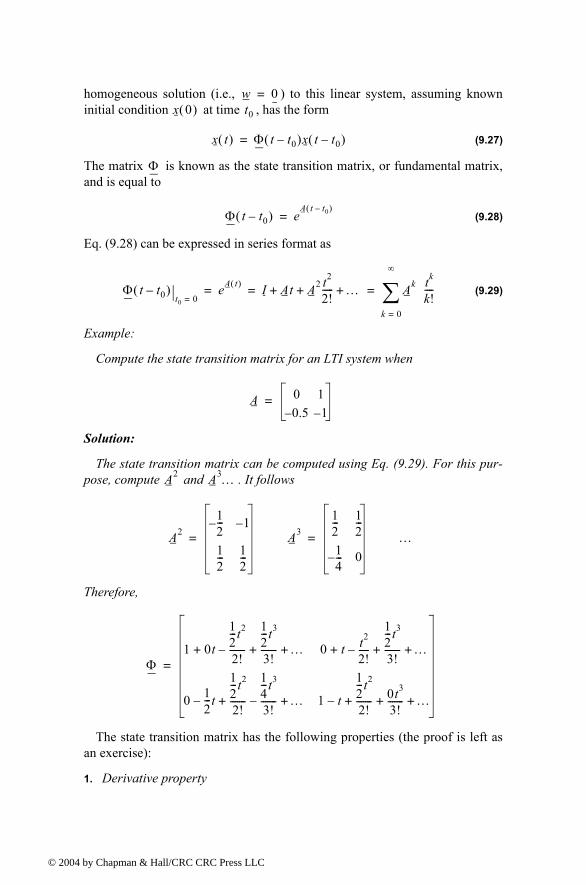
homogeneous solution (i.e., ) to this linear system, assuming knowninitial condition at time , has the form

(9.27)

The matrix is known as the state transition matrix, or fundamental matrix,and is equal to

(9.28)

Eq. (9.28) can be expressed in series format as

(9.29)

Example:

Compute the state transition matrix for an LTI system when

Solution:

The state transition matrix can be computed using Eq. (9.29). For this pur-pose, compute and . It follows

Therefore,

The state transition matrix has the following properties (the proof is left asan exercise):

1. Derivative property

w 0=x 0( ) t0

x t( ) Φ t t0�( )x t t0�( )=

Φ

Φ t t0�( ) eA t t0�( )

=

Φ t t0�( )t0 0=

eA t( ) I At A2 t2

2!----- …+ + + Ak tk

k!----

k 0=

∞

∑= = =

A 0 10.5� 1�

=

A2 A3…

A212---� 1�

12--- 1

2---

= A312--- 1

2---

14---� 0

= …

Φ1 0t

12---t2

2!-------

12---t3

3!------- …+ +�+ 0 t t2

2!-----

12--- t3

3!------- …+ +�+

0 12---t

12---t2

2!-------+�

14---t3

3!------- …+� 1 t�

12---t2

2!------- 0t3

3!------- …+ + +

=


© 200

(9.30)

2. Identity property

(9.31)

3. Initial value property

(9.32)

4. Transition property

(9.33)

5. Inverse property

(9.34)

6. Separation property

(9.35)

The general solution to the system defined in Eq. (9.25) can be written as

(9.36)

The first term of the right-hand side of Eq. (9.36) represents the contributionfrom the system response to the initial condition. The second term is the contri-bution due to the driving force . By combining Eqs. (9.26) and (9.36) anexpression for the output is computed as

(9.37)

Note that the system impulse response is equal to .

The difference equations describing a discrete time system, equivalent toEqs. (9.25) and (9.26), are

(9.38)

(9.39)

t∂∂ Φ t t0�( ) AΦ t t0�( )=

Φ t0 t0�( ) Φ 0( ) I= =

t∂∂ Φ t t0�( )

t t0=

A=

Φ t2 t0�( ) Φ t2 t1�( )Φ t1 t0�( )= t0 t1 t2≤ ≤;

Φ t0 t1�( ) Φ1�

t1 t0�( )=

Φ t1 t0�( ) Φ t1( )Φ1�

t0( )=

x t( ) Φ t t0�( )x t0( ) Φ t τ�( )Bw τ( ) τd

t0

t

∫+=

w

y t( ) CeA t t0�( )

x t0( ) CeA t τ�( )B Dδ t τ�( )�[ ]w τ( ) τd

t0

t

∫+=

CeAtB Dδ t( )�

x n 1+( ) A x n( ) Bw n( )+=

y n( ) C x n( ) Dw n( )+=


© 200

where defines the discrete time and is the sampling interval. All othervectors and matrices were defined earlier. The homogeneous solution to thesystem defined in Eq. (9.38), with initial condition , is

(9.40)

In this case the state transition matrix is an matrix given by

(9.41)

The following is the list of properties associated with the discrete transitionmatrix

(9.42)

(9.43)

(9.44)

(9.45)

(9.46)

(9.47)

The solution to the general case (i.e., non-homogeneous system) is given by

(9.48)

It follows that the output is given by

(9.49)

where the system impulse response is given by

(9.50)

Taking the Z-transform for Eqs. (9.38) and (9.39) yields

n nT T

x n0( )

x n( ) An n0�

x n0( )=

n n×

Φ n n0,( ) Φ n n0�( ) An n0�

= =

Φ n 1 n0�+( ) AΦ n n0�( )=

Φ n0 n0�( ) Φ 0( ) I= =

Φ n0 1 n0�+( ) Φ 1( ) A= =

Φ n2 n0�( ) Φ n2 n1�( )Φ n1 n0�( )=

Φ n0 n1�( ) Φ1�

n1 n0�( )=

Φ n1 n0�( ) Φ n1( )Φ1�

n0( )=

x n( ) Φ n n0�( )x n0( ) Φ n m 1��( )Bw m( )

m n0=

n 1�

∑+=

y n( ) CΦ n n0�( )x n0( ) C Φ n m 1��( )Bw m( ) Dw n( )+

m n0=

n 1�

∑+=

h n( ) C Φ n m 1��( )Bδ m( ) Dδ n( )+

m n0=

n 1�

∑=


© 200

(9.51)

(9.52)

Manipulating Eqs. (9.51) and (9.52) yields

(9.53)

(9.54)

It follows that the state transition matrix is

(9.55)

and the system impulse response in the z-domain is

(9.56)

9.7. The LTI System of Interest For the purpose of establishing the framework necessary for the Kalman fil-

ter development, consider the LTI system shown in Fig. 9.18. This system(which is a special case of the system described in the previous section) can bedescribed by the following first order differential vector equations

(9.57)

(9.58)

where is the observable part of the system (i.e., output), is a driving force,and is the measurement noise. The matrices and vary depending on thesystem. The noise observation is assumed to be uncorrelated. If the initialcondition vector is , then from Eq. (9.36) we get

(9.59)

The object (abstract) is observed only at discrete times determined by thesystem. These observation times are declared by discrete time where isthe sampling interval. Using the same notation adopted in the previous section,the discrete time representations of Eqs. (9.57) and (9.58) are

(9.60)

zx z( ) Ax z( ) Bw z( ) zx 0( )+ +=

y z( ) Cx z( ) Dw z( )+=

x z( ) zI A�[ ] 1� Bw z( ) zI A�[ ] 1� zx 0( )+=

y z( ) C zI A�[ ] 1� B D+{ }w z( ) C zI A�[ ] 1� zx 0( )+=

Φ z( ) z zI A�[ ] 1� I z 1� A�[ ]1�

= =

h z( ) CΦ z( )z 1� B D+=

x· t( ) A x t( ) u t( )+=

y t( ) G x t( ) v t( )+=

y uv A G

vx t0( )

x t( ) Φ t t0�( )x t0( ) Φ t τ�( )u τ( ) τd

t0

t

∫+=

nT T

x n( ) A x n 1�( ) u n( )+=


© 200

(9.61)

The homogeneous solution to this system is given in Eq. (9.27) for continuoustime, and in Eq. (9.40) for discrete time.

The state transition matrix corresponding to this system can be obtainedusing Taylor series expansion of the vector . More precisely,

(9.62)

It follows that the elements of the state transition matrix are defined by

(9.63)

Using matrix notation, the state transition matrix is then given by

(9.64)

The matrix given in Eq. (9.64) is often called the Newtonian matrix.

y n( ) G x n( ) v n( )+=

Σ Σu

A

∫ Gy

x t0( )

x

v

Figure 9.18. An LTI system.

x

x x Tx· T2

2!-----x·· …+ + +=

x· x· Tx·· …+ +=

x·· x·· …+=

Φ ij[ ] Tj i� j i�( )!÷ 1 i j n≤,≤0 j i<

=

Φ

1 T T2

2!----- …

0 1 T …0 0 1 …… … … …

=


© 200

9.8. Fixed-Gain Tracking Filters This class of filters (or estimators) is also known as �Fixed-Coefficient� fil-

ters. The most common examples of this class of filters are the and filters and their variations. The and trackers are one-dimensional sec-ond and third order filters, respectively. They are equivalent to special cases ofthe one-dimensional Kalman filter. The general structure of this class of esti-mators is similar to that of the Kalman filter.

The standard filter provides smoothed and predicted data for targetposition, velocity (Doppler), and acceleration. It is a polynomial predictor/cor-rector linear recursive filter. This filter can reconstruct position, velocity, andconstant acceleration based on position measurements. The filter can alsoprovide a smoothed (corrected) estimate of the present position which can beused in guidance and fire control operations.

Notation:

For the purpose of the discussion presented in the remainder of this chapter,the following notation is adopted: represents the estimate during the

sampling interval, using all data up to and including the samplinginterval; is the measured value; and is the residual (error).

The fixed-gain filter equation is given by

(9.65)

Since the transition matrix assists in predicting the next state,

(9.66)

Substituting Eq. (9.66) into Eq. (9.65) yields

(9.67)

The term enclosed within the brackets on the right hand side of Eq. (9.67) isoften called the residual (error) which is the difference between the measuredinput and predicted output. Eq. (9.67) means that the estimate of is thesum of the prediction and the weighted residual. The term repre-sents the prediction state. In the case of the estimator, is the row vectorgiven by

(9.68)

and the gain matrix is given by

αβ αβγαβ αβγ

αβγ

αβγ

x n m( )nth mth

yn nth en nth

x n n( ) Φx n 1� n 1�( ) K yn GΦx n 1� n 1�( )�[ ]+=

x n 1+ n( ) Φx n n( )=

x n n( ) x n n 1�( ) K yn Gx n n 1�( )�[ ]+=

x n( )Gx n n 1�( )

αβγ G

G 1 0 0 …=

K


© 200

(9.69)

One of the main objectives of a tracking filter is to decrease the effect of thenoise observation on the measurement. For this purpose the noise covariancematrix is calculated. More precisely, the noise covariance matrix is

(9.70)

where indicates the expected value operator. Noise is assumed to be a zeromean random process with variance equal to . Additionally, noise measure-ments are also assumed to be uncorrelated,

(9.71)

Eq. (9.65) can be written as

(9.72)

where

(9.73)

Substituting Eqs. (9.72) and (9.73) into Eq. (9.70) yields

(9.74)

Expanding the right hand side of Eq. (9.74) and using Eq. (9.71) give

(9.75)

Under the steady state condition, Eq. (9.75) collapses to

(9.76)

where is the steady state noise covariance matrix. In the steady state,

(9.77)

Several criteria can be used to establish the performance of the fixed-gaintracking filter. The most commonly used technique is to compute the VarianceReduction Ratio (VRR). The VRR is defined only when the input to the trackeris noise measurements. It follows that in the steady state case, the VRR is the

Kαβ T⁄

γ T2⁄

=

C n n( ) E x n n( )( )xt n n( ){ }= yn; vn=

Eσv

2

E vnvm{ }δσv

2 n m=

0 n m≠

=

x n n( ) Ax n 1� n 1�( ) Kyn+=

A I KG�( )Φ=

C n n( ) E Ax n 1� n 1�( ) Kyn+( ) Ax n 1� n 1�( ) Kyn+( )t{ }=

C n n( ) AC n 1� n 1�( )At Kσv2Kt+=

C n n( ) ACAt Kσv2Kt+=

C

C n n( ) C n 1� n 1�( ) C= = for any n


© 200

steady state ratio of the output variance (auto-covariance) to the input measure-ment variance.

In order to determine the stability of the tracker under consideration, con-sider the Z-transform for Eq. (9.72),

(9.78)

Rearranging Eq. (9.78) yields the following system transfer functions:

(9.79)

where is called the characteristic matrix. Note that the system trans-fer functions can exist only when the characteristic matrix is a non-singularmatrix. Additionally, the system is stable if and only if the roots of the charac-teristic equation are within the unit circle in the z-plane,

(9.80)

The filter�s steady state errors can be determined with the help of Fig. 9.19.The error transfer function is

(9.81)

and by using Abel�s theorem, the steady state error is

(9.82)

Substituting Eq. (9.82) into (9.81) yields

(9.83)

x z( ) Az 1� x z( ) Kyn z( )+=

h z( ) x z( )yn z( )------------ I Az 1��( )

1�K= =

I Az 1��( )

I Az 1��( ) 0=

e z( )y z( )

1 h z( )+-------------------=

e∞ e t( )t ∞→lim z 1�

z----------- e z( )

z 1→lim= =

e∞z 1�

z-----------

y z( )1 h z( )+-------------------

z 1→lim=

Σy z( ) x z( )

h z( )e z( )+ -

Figure 9.19. Steady state error computation.


© 200

9.8.1. The Filter

The tracker produces, on the observation, smoothed estimates forposition and velocity, and a predicted position for the observation.Fig. 9.20 shows an implementation of this filter. Note that the subscripts �p�and �s� are used to indicate, respectively, the predicated and smoothed values.The tracker can follow an input ramp (constant velocity) with no steadystate errors. However, a steady state error will accumulate when constantacceleration is present in the input. Smoothing is done to reduce errors in thepredicted position through adding a weighted difference between the measuredand predicted values to the predicted position, as follows:

(9.84)

(9.85)

is the position input samples. The predicted position is given by

(9.86)

The initialization process is defined by

A general form for the covariance matrix was developed in the previous sec-tion, and is given in Eq. (9.75). In general, a second order one-dimensionalcovariance matrix (in the context of the filter) can be written as

(9.87)

where, in general, is

(9.88)

By inspection, the filter has

(9.89)

αβαβ nth

n 1+( )th

αβ

xs n( ) x n n( ) xp n( ) α x0 n( ) xp n( )�( )+= =

x· s n( ) x' n n( ) x· s n 1�( ) βT--- x0 n( ) xp n( )�( )+= =

x0

xp n( ) xs n n 1�( ) xs n 1�( ) Tx· s n 1�( )+= =

xs 1( ) xp 2( ) x0 1( )= =

x· s 1( ) 0=

x· s 2( )x0 2( ) x0 1( )�

T--------------------------------=

αβ

C n n( )Cxx Cxx·

Cx· x Cx· x·=

Cxy

Cxy E xyt{ }=

αβ

A 1 α� 1 α�( )Tβ� T⁄ 1 β�( )

=


© 200

(9.90)

(9.91)

(9.92)

Finally, using Eqs. (9.89) through (9.92) in Eq. (9.72) yields the steady statenoise covariance matrix,

(9.93)

It follows that the position and velocity VRR ratios are, respectively, given by

(9.94)

(9.95)

The stability of the filter is determined from its system transfer func-tions. For this purpose, compute the roots for Eq. (9.80) with from Eq.(9.89),

K αβ T⁄

=

G 1 0=

Φ 1 T0 1

=

Σ

Σ Σ Σ

delay, z 1�

delay, z 1�

T

α

βT---

-

+ ++

++

++

xp n( )

x· s n( )

xs n( )

x0 n( )

Figure 9.20. An implementation of an tracker.αβ

Cσv

2

α 4 2α β��( )----------------------------------

2α2 3αβ� 2β+β 2α β�( )

T------------------------

β 2α β�( )T

------------------------ 2β2

T2--------

=

VRR( )x Cxx σv2⁄ 2α2 3αβ� 2β+

α 4 2α β��( )---------------------------------------= =

VRR( )x· Cx· x· σv2⁄ 1

T2----- 2β2

α 4 2α β��( )----------------------------------= =

αβA


© 200

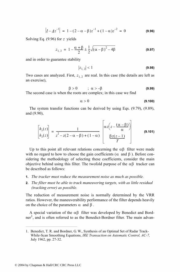
(9.96)

Solving Eq. (9.96) for yields

(9.97)

and in order to guarantee stability

(9.98)

Two cases are analyzed. First, are real. In this case (the details are left asan exercise),

(9.99)The second case is when the roots are complex; in this case we find

(9.100)

The system transfer functions can be derived by using Eqs. (9.79), (9.89),and (9.90),

(9.101)

Up to this point all relevant relations concerning the filter were madewith no regard to how to choose the gain coefficients ( and ). Before con-sidering the methodology of selecting these coefficients, consider the mainobjective behind using this filter. The twofold purpose of the tracker canbe described as follows:

1. The tracker must reduce the measurement noise as much as possible.2. The filter must be able to track maneuvering targets, with as little residual

(tracking error) as possible.

The reduction of measurement noise is normally determined by the VRRratios. However, the maneuverability performance of the filter depends heavilyon the choice of the parameters and .

A special variation of the filter was developed by Benedict and Bord-ner1, and is often referred to as the Benedict-Bordner filter. The main advan-

1. Benedict, T. R. and Bordner, G. W., Synthesis of an Optimal Set of Radar Track-While-Scan Smoothing Equations, IRE Transaction on Automatic Control, AC-7, July 1962, pp. 27-32.

I Az 1�� 1 2 α� β�( )z 1�� 1 α�( )z 2�+ 0= =

z

z1 2, 1 α β+2

------------- 12--- α β�( )2 4β�±�=

z1 2, 1<

z1 2,

β 0> α β�>;

α 0>

hx z( )hx· z( )

1z2 z 2 α� β�( )� 1 α�( )+----------------------------------------------------------------

αz z α β�( )α

-----------------�

βz z 1�( )T

----------------------=

αβα β

αβ

α β

αβ


© 200

tage of the Benedict-Bordner is reducing the transient errors associated withthe tracker. This filter uses both the position and velocity VRR ratios asmeasures of performance. It computes the sum of the squared differencesbetween the input (position) and the output when the input has a unit stepvelocity at time zero. Additionally, it computes the squared differencesbetween the real velocity and the velocity output when the input is as describedearlier. Both error differences are minimized when

(9.102)

In this case, the position and velocity VRR ratios are, respectively, given by

(9.103)

(9.104)

Another important sub-class of the tracker is the critically damped filter,often called the fading memory filter. In this case, the filter coefficients arechosen on the basis of a smoothing factor , where . The gain coeffi-cients are given by

(9.105)

(9.106)

Heavy smoothing means and little smoothing means . The ele-ments of the covariance matrix for a fading memory filter are

(9.107)

(9.108)

(9.109)

9.8.2. The Filter

The tracker produces, for the observation, smoothed estimates ofposition, velocity, and acceleration. It also produces the predicted position and

αβ

β α2

2 α�------------=

VRR( )xα 6 5α�( )

α2 8α 8+�----------------------------=

VRR( )x·2T2----- α3 2 α�( )⁄

α2 8α 8+�----------------------------=

αβ

ξ 0 ξ 1≤ ≤

α 1 ξ2�=

β 1 ξ�( )2=

ξ 1→ ξ 0→

Cxx1 ξ�

1 ξ+( )3------------------- 1 4ξ 5ξ2+ +( ) σv

2=

Cxx· Cx· x1T--- 1 ξ�

1 ξ+( )3------------------- 1 2ξ 3ξ2+ +( ) σv

2= =

Cx· x·2T2----- 1 ξ�

1 ξ+( )3------------------- 1 ξ�( )2 σv

2=

αβγαβγ nth


© 200

velocity for the observation. An implementation of the trackeris shown in Fig. 9.21.

The tracker will follow an input whose acceleration is constant with nosteady state errors. Again, in order to reduce the error at the output of thetracker, a weighted difference between the measured and predicted values isused in estimating the smoothed position, velocity, and acceleration as follows:

(9.110)

(9.111)

(9.112)

(9.113)

and the initialization process is

n 1+( )th αβγ

αβγ

xs n( ) xp n( ) α x0 n( ) xp n( )�( )+=

x· s n( ) x· s n 1�( ) Tx··s n 1�( ) βT--- x0 n( ) xp n( )�( )+ +=

x··s n( ) x··s n 1�( ) 2γT2----- x0 n( ) xp n( )�( )+=

xp n 1+( ) xs n( ) T x· s n( ) T2

2----- x··s n( )+ +=

xs 1( ) xp 2( ) x0 1( )= =

x· s 1( ) x··s 1( ) x··s 2( ) 0= = =

x· s 2( )x0 2( ) x0 1( )�

T--------------------------------=

Σ

Σ Σ Σdelay, z 1�α

βT---

-+

+ xp

x·px· s

xs

x0

Figure 9.21. An implementation for an tracker.αβγ

Σ

2γT2-----

T

T2 2⁄ T

Σ

x··s

delay, z 1�

delay, z 1�

+++

++ +

+

+

++


© 200

Using Eq. (9.63) the state transition matrix for the filter is

(9.114)

The covariance matrix (which is symmetric) can be computed from Eq. (9.76).For this purpose, note that

(9.115)

(9.116)

and

(9.117)

Substituting Eq. (9.117) into (9.76) and collecting terms the VRR ratios arecomputed as

(9.118)

(9.119)

(9.120)

As in the case of any discrete time system, this filter will be stable if and only ifall of its poles fall within the unit circle in the z-plane.

The characteristic equation is computed by setting

x··s 3( )x0 3( ) x0 1( ) 2x0 2( )�+

T2-------------------------------------------------------=

αβγ

Φ1 T T2

2-----

0 1 T0 0 1

=

Kαβ T⁄

γ T2⁄

=

G 1 0 0=

A I KG�( )Φ1 α� 1 α�( )T 1 α�( )T2 2⁄β T⁄� β� 1+ 1 β 2⁄�( )T

2γ� T2⁄ 2γ� T⁄ 1 γ�( )

= =

VRR( )x2β 2α2 2β 3αβ�+( ) αγ 4 2α� β�( )�

4 2α� β�( ) 2αβ αγ 2γ�+( )----------------------------------------------------------------------------------------------=

VRR( )x·4β3 4β2γ� 2γ2 2 α�( )+

T2 4 2α� β�( ) 2αβ αγ 2γ�+( )-----------------------------------------------------------------------------=

VRR( )x··4βγ2

T4 4 2α� β�( ) 2αβ αγ 2γ�+( )-----------------------------------------------------------------------------=

αβγ


© 200

(9.121)

Substituting Eq. (9.117) into (9.121) and collecting terms yield the followingcharacteristic function:

(9.122)

The becomes a Benedict-Bordner filter when

(9.123)

Note that for Eq. (9.123) reduces to Eq. (9.102). For a critically dampedfilter the gain coefficients are

(9.124)

(9.125)

(9.126)

Note that heavy smoothing takes place when , while means thatno smoothing is present.

MATLAB Function �ghk_tracker.m�

The function �ghk_tracker.m� implements the steady state filter. It isgiven in Listing 9.2 in Section 9.11. The syntax is as follows:

[residual, estimate] = ghk_tracker (X0, smoocof, inp, npts, T, nvar)

where

Symbol Description Status

X0 initial state vector input

smoocof desired smoothing coefficient input

inp array of position measurements input

npts number of points in input position input

T sampling interval input

nvar desired noise variance input

residual array of position error (residual) output

estimate array of predicted position output

I Az 1�� 0=

f z( ) z3 3α� β γ+ +( )z2 3 β� 2α� γ+( )z 1 α�( )�+ +=

αβγ

2β α α β γ2---+ +

� 0=

γ 0=

α 1 ξ3�=

β 1.5 1 ξ2�( ) 1 ξ�( ) 1.5 1 ξ�( )2 1 ξ+( )= =

γ 1 ξ�( )3=

ξ 1→ ξ 0=

αβγ


© 200

Note that �ghk_tracker.m� uses MATLAB�s function �normrnd.m� to gener-ate zero mean Gaussian noise, which is part of MATLAB�s Statistics Toolbox.If this toolbox is not available to the user, then �ghk_tracker.m� function-callmust be modified to

[residual, estimate] = ghk_tracker1 (X0, smoocof, inp, npts, T)

which is also part of Listing 9.2. In this case, noise measurements are either tobe considered unavailable or are part of the position input array.

To illustrate how to use the functions ghk_tracker.m and ghk_tracker1.m,consider the inputs shown in Figs. 9.22 and 9.23. Fig. 9.22 assumes an inputwith lazy maneuvering, while Fig. 9.23 assumes an aggressive maneuveringcase. For this purpose, the program called �fig9_21.m� was written. It is givenin Listing 9.3 in Section 9.11.

Figs. 9.24 and 9.25 show the residual error and predicted position corre-sponding (generated using the program �fig9_21.m�) to Fig. 9.22 for twocases: heavy smoothing and little smoothing with and without noise. The noiseis white Gaussian with zero mean and variance of . Figs. 9. 26 and9.27 show the residual error and predicted position corresponding (generatedusing the program �fig9_20.m�) to Fig. 9.23 with and without noise.

σv2 0.05=

Figure 9.22. Position (truth-data); lazy maneuvering.

5 0 0 1 0 0 0 1 50 0 2 0 0 0 2 5 0 0 3 0 0 0 3 5 0 0 4 0 0 0 4 5 0 0 5 0 0 01

1 .5

2

2 .5

Po

sit

ion

S a m p le n u m b e r


© 200

Figure 9.23. Position (truth-data); aggressive maneuvering.

0 1 0 0 0 2 0 0 0 3 0 0 0 4 0 0 0 5 0 0 0 6 0 0 00

0 .5

1

1 .5

2

2 .5

3

3 .5


Po

sit

ion

Figure 9.24a-1. Predicted and true position. (i.e., large gain coefficients). No noise present.

ξ 0.1=

50 0 1 00 0 1 5 00 2 0 00 25 0 0 3 00 0 3 50 0 4 00 0 45 001

1 .5

2

Pre

dic

ted

po

sit

ion

5 0 0 1 00 0 1 5 00 2 0 00 25 0 0 3 00 0 3 50 0 4 00 0 45 001

1 .5

2


Po

sit

ion

- t

ruth


© 200

Figure 9.24a-2. Position residual (error). Large gain coefficients. No noise. The error settles to zero fairly quickly.

0 5 10 15 20 25 30 35 40 45 50-1 .5

-1

-0 .5

0

0 .5

1

1 .5

2

S am p le num ber

Re

sid

ua

l

Figure 9.24b-1. Predicted and true position. (i.e., small gain coefficients). No noise present.

ξ 0.9=

5 0 0 1 0 0 0 1 5 0 0 2 0 0 0 2 5 0 0 3 0 0 0 3 5 0 0 4 0 0 0 4 5 0 0

1

1 .5

2

Pre

dic

ted

po

sit

ion

5 0 0 1 0 0 0 1 5 0 0 2 0 0 0 2 5 0 0 3 0 0 0 3 5 0 0 4 0 0 0 4 5 0 01

1 .5

2


Po

sit

ion

- t

ruth


© 200

Figure 9.24b-2. Position residual (error). Small gain coefficients. No noise. It takes the filter longer time for the error to settle down.

0 5 0 1 0 0 1 5 0 2 0 0 2 5 0 3 0 0 3 5 0 4 0 0 4 5 0 5 0 0-1 .2

-1

-0 .8

-0 .6

-0 .4

-0 .2

0

0 .2


Re

sid

ua

l e

rro

r

Figure 9.25a-1. Predicted and true position. (i.e., large gain coefficients). Noise is present.

ξ 0.1=

50 0 1 00 0 1 5 00 2 0 00 25 0 0 3 00 0 3 50 0 4 00 0 45 00

1

1 .5

2

2 .5

Pre

dic

ted

po

sit

ion

5 0 0 1 00 0 1 5 00 2 0 00 25 0 0 3 00 0 3 50 0 4 00 0 45 001

1 .5

2


Po

sit

ion

- t

ruth


© 200

Figure 9.25a-2. Position residual (error). Large gain coefficients. Noise present. The error settles down quickly. The variation is due to noise.

0 50 1 00 15 0 20 0 250 3 00 3 50 40 0 45 0 5 00-1 .5

-1

-0 .5

0

0 .5

1

1 .5

2

S am p le nu m be r

Re

sid

ua

l e

rro

r

Figure 9.25b-1. Predicted and true position. (i.e., small gain coefficients). Noise is present.

ξ 0.9=

5 0 0 1 0 0 0 1 5 0 0 2 0 0 0 2 5 0 0 3 0 0 0 3 5 0 0 4 0 0 0 4 5 0 0

1

1 .5

2

2 .5

Pre

dic

ted

po

sit

ion

5 0 0 1 0 0 0 1 5 0 0 2 0 0 0 2 5 0 0 3 0 0 0 3 5 0 0 4 0 0 0 4 5 0 01

1 .5

2


Po

sit

ion

- t

ruth


© 200

Figure 9.25b-2. Position residual (error). Small gain coefficients. Noise present. The error requires more time before settling down. The variation is due to noise.

0 500 1000 1500-1 .2

-1

-0 .8

-0 .6

-0 .4

-0 .2

0

0 .2

0 .4

S am p le num ber

Re

sid

ua

l

Figure 9.26a. Predicted and true position. (i.e., large gain coefficients). Noise is present.

ξ 0.1=

500 1000 1500 2000 2500 3000 3500 4000 4500

0 .5

1

1 .5

2

2 .5

3

Pre

dic

ted

po

sit

ion

5 00 1000 1500 2000 2500 3000 3500 4000 4500

0 .5

1

1 .5

2

2 .5

3

S am p le num ber

Po

sit

ion

- t

ruth


© 200

Figure 9.26b. Position residual (error). Large gain coefficients. No noise. The error settles down quickly.

0 5 10 1 5 20 25 30 35 4 0 4 5 50-2 .5

-2

-1 .5

-1

-0 .5

0

0 .5

1

1 .5x 10

-3R

es

idu

al

S a m p le num be r

Figure 9.27a. Predicted and true position. (i.e., small gain coefficients). Noise is present.

ξ 0.8=

5 0 0 1 0 0 0 1 5 0 0 2 0 0 0 2 5 0 0 3 0 0 0 3 5 0 0 4 0 0 0 4 5 0 00

1

2

3

Pre

dic

ted

po

sit

ion

5 0 0 1 0 0 0 1 5 0 0 2 0 0 0 2 5 0 0 3 0 0 0 3 5 0 0 4 0 0 0 4 5 0 0

0 .5

1

1 .5

2

2 .5

3


Po

sit

ion

- t

ruth


© 200

9.9. The Kalman FilterThe Kalman filter is a linear estimator that minimizes the mean squared error

as long as the target dynamics are modeled accurately. All other recursive fil-ters, such as the and the Benedict-Bordner filters, are special cases of thegeneral solution provided by the Kalman filter for the mean squared estimationproblem. Additionally, the Kalman filter has the following advantages:

1. The gain coefficients are computed dynamically. This means that the same filter can be used for a variety of maneuvering target environments.

2. The Kalman filter gain computation adapts to varying detection histories, including missed detections.

3. The Kalman filter provides an accurate measure of the covariance matrix. This allows for better implementation of the gating and association pro-cesses.

4. The Kalman filter makes it possible to partially compensate for the effects of mis-correlation and mis-association.

Many derivations of the Kalman filter exist in the literature; only results areprovided in this chapter. Fig. 9.28 shows a block diagram for the Kalman filter.

Figure 9.27b. Position residual (error). Small gain coefficients. Noise present. The error stays fairly large; however, its average is around zero. The variation is due to noise.

0 50 100 150 200 250 300 350 400 450 500-0 .2

-0 .15

-0 .1

-0 .05

0

0 .05

0 .1

0 .15

0 .2

S am p le num ber

Re

sid

ua

l e

rro

r

αβγ


© 200

The Kalman filter equations can be deduced from Fig. 9.28. The filtering equa-tion is

(9.127)

The measurement vector is

(9.128)

where is zero mean, white Gaussian noise with covariance ,

(9.129)

The gain (weight) vector is dynamically computed as

(9.130)

where the measurement noise matrix represents the predictor covariancematrix, and is equal to

(9.131)

where is the covariance matrix for the input ,

(9.132)

x n n( ) xs n( ) x n n 1�( ) K n( ) y n( ) Gx n n 1�( )�[ ]+= =

y n( ) Gx n( ) v n( )+=

v n( ) ℜc

ℜc E y n( ) yt n( ){ }=

Σu

Φ

G

y

xs n 1+( )v

z 1�

z 1�

Σ ΣK

G Φ

+- + + xs n( )

Figure 9.28. Structure of the Kalman filter.

K n( ) P n n 1�( )Gt GP n n 1�( )Gt ℜc+[ ]1�

=

P

P n 1+ n( ) E xs n 1+( )x∗s n( ){ } ΦP n n( )Φt

Q+= =

Q u

Q E u n( ) ut n( ){ }=


© 200

The corrector equation (covariance of the smoothed estimate) is

(9.133)

Finally, the predictor equation is

(9.134)

9.9.1. The Singer -Kalman Filter

The Singer1 filter is a special case of the Kalman where the filter is gov-erned by a specified target dynamic model whose acceleration is a random pro-cess with autocorrelation function given by

(9.135)

where is the correlation time of the acceleration due to target maneuveringor atmospheric turbulence. The correlation time may vary from as low as10 seconds for aggressive maneuvering to as large as 60 seconds for lazymaneuvering cases.

Singer defined the random target acceleration model by a first order Markovprocess given by

(9.136)

where is a zero mean, Gaussian random variable with unity variance, is the maneuver standard deviation, and the maneuvering correlation coef-

ficient is given by

(9.137)

The continuous time domain system that corresponds to these conditions is thesame as the Wiener-Kolmogorov whitening filter which is defined by the dif-ferential equation

(9.138)

1. Singer, R. A., Estimating Optimal Tracking Filter Performance for Manned Maneu-vering Targets, IEEE Transaction on Aerospace and Electronics, AES-5, July, 1970, pp. 473-483.

P n n( ) I K n( )G�[ ]P n n 1�( )=

x n 1+ n( ) Φx n n( )=

αβγ

E x·· t( ) x·· t t1+( ){ } σa2 e

t1τm------�

=

τmτm

x·· n 1+( ) ρm x·· n( ) 1 ρm2� σm w n( )+=

w n( )σm

ρm

ρm eTτm-----�

=

tdd v t( ) βmv t( )� w t( )+=


© 200

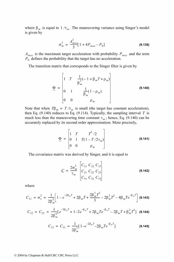
where is equal to . The maneuvering variance using Singer�s modelis given by

(9.139)

is the maximum target acceleration with probability and the term defines the probability that the target has no acceleration.

The transition matrix that corresponds to the Singer filter is given by

(9.140)

Note that when is small (the target has constant acceleration),then Eq. (9.140) reduces to Eq. (9.114). Typically, the sampling interval ismuch less than the maneuvering time constant ; hence, Eq. (9.140) can beaccurately replaced by its second order approximation. More precisely,

(9.141)

The covariance matrix was derived by Singer, and it is equal to

(9.142)

where

(9.143)

(9.144)

(9.145)

βm 1 τm⁄

σm2 Amax

2

3----------- 1 4Pmax P0�+[ ]=

Amax PmaxP0

Φ

1 T 1βm

2------ 1� βmT ρm+ +( )

0 1 1βm------ 1 ρm�( )

0 0 ρm

=

Tβm T τm⁄=T

τm

Φ1 T T2 2⁄0 1 T 1 T 2τm⁄�( )

0 0 ρm

=

C2σm

2

τm----------

C11 C12 C13

C21 C22 C23

C31 C32 C33

=

C11 σx2 1

2βm5

--------- 1 e2βmT�

� 2βmT2βm

3 T3

3--------------- 2βm

2 T2� 4βmTeβmT�

�+ += =

C12 C211

2βm4

--------- e2βmT�

1+ 2� eβmT�

2βmTeβmT�

2βmT βm2 T2+�+[ ]= =

C13 C311

2βm3

--------- 1 e2βmT�

� 2� βmTeβmT�

[ ]= =


© 200

(9.146)

(9.147)

(9.148)

Two limiting cases are of interest:

1. The short sampling interval case ( ),

(9.149)

and the state transition matrix is computed from Eq. (9.141) as

(9.150)

which is the same as the case for the filter (constant acceleration).

2. The long sampling interval ( ). This condition represents the case when acceleration is a white noise process. The corresponding covariance and transition matrices are, respectively, given by

(9.151)

(9.152)

Note that under the condition that , the cross correlation terms and become very small. It follows that estimates of acceleration are no longer

C221

2βm3

--------- 4eβmT�

3� e2βmT�

� 2βmT+[ ]=

C23 C321

2βm2

--------- e2βmT�

1 2eβmT�

�+[ ]= =

C331

2βm--------- 1 e

2βmT��[ ]=

T τm«

CβmT 0→

lim2σm

2

τm----------

T5 20⁄ T4 8⁄ T3 6⁄

T4 8⁄ T3 3⁄ T2 2⁄

T3 6⁄ T2 2⁄ T

=

ΦβmT 0→

lim1 T T2 2⁄0 1 T0 0 1

=

αβγ

T τm»

CβmT ∞→

lim σm2

2T3τm

3--------------- T2τm τm

2

T2τm 2Tτm τm

τm2 τm 1

=

ΦβmT ∞→

lim1 T Tτm

0 1 τm

0 0 0

=

T τm» C13C23


© 200

available, and thus a two state filter model can be used to replace the three statemodel. In this case,

(9.153)

(9.154)

9.9.2. Relationship between Kalman and Filters

The relationship between the Kalman filter and the filters can be easilyobtained by using the appropriate state transition matrix , and gain vector corresponding to the in Eq. (9.127). Thus,

(9.155)

with (see Fig. 9.21)

(9.156)

(9.157)

(9.158)

Comparing the previous three equations with the filter equations yields

(9.159)

Additionally, the covariance matrix elements are related to the gain coeffi-cients by

C 2σm2 τm

T3 3⁄ T2 2⁄

T2 2⁄ T=

Φ 1 T0 1

=

αβγαβγΦ K

αβγ

x n n( )x· n n( )x·· n n( )

x n n 1�( )x· n n 1�( )x·· n n 1�( )

k1 n( )

k2 n( )

k3 n( )

x0 n( ) x n n 1�( )�[ ]+=

x n n 1�( ) xs n 1�( ) T x· s n 1�( ) T2

2----- x··s n 1�( )+ +=

x· n n 1�( ) x· s n 1�( ) T x··s n 1�( )+=

x·· n n 1�( ) x··s n 1�( )=

αβγ

αβT---

γ

T2-----

k1

k2

k3

=


© 200

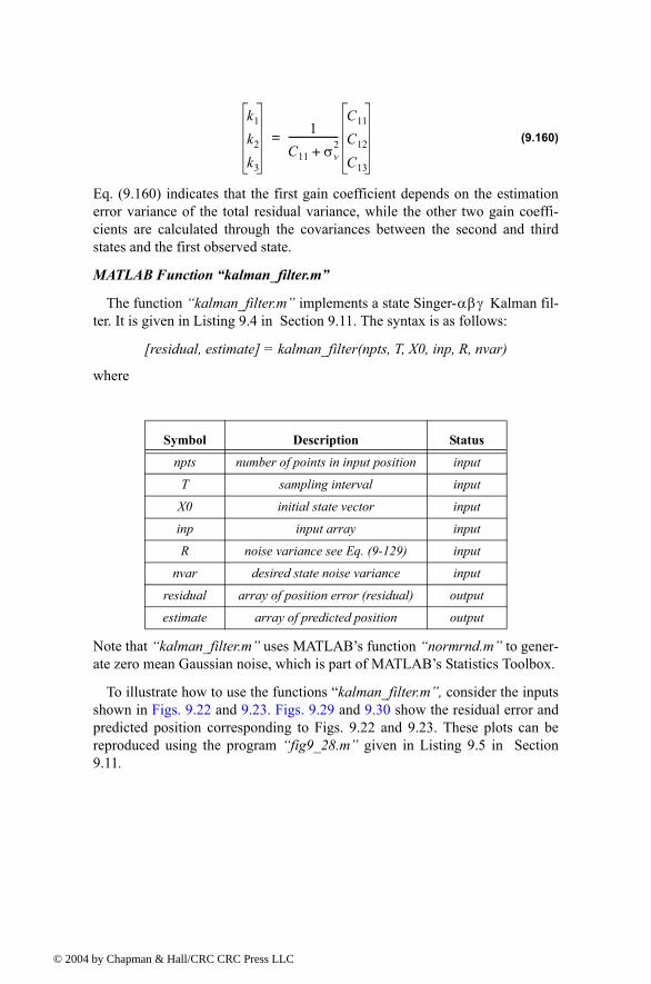
(9.160)

Eq. (9.160) indicates that the first gain coefficient depends on the estimationerror variance of the total residual variance, while the other two gain coeffi-cients are calculated through the covariances between the second and thirdstates and the first observed state.

MATLAB Function �kalman_filter.m�

The function �kalman_filter.m� implements a state Singer- Kalman fil-ter. It is given in Listing 9.4 in Section 9.11. The syntax is as follows:

[residual, estimate] = kalman_filter(npts, T, X0, inp, R, nvar)

where

Note that �kalman_filter.m� uses MATLAB�s function �normrnd.m� to gener-ate zero mean Gaussian noise, which is part of MATLAB�s Statistics Toolbox.

To illustrate how to use the functions �kalman_filter.m�, consider the inputsshown in Figs. 9.22 and 9.23. Figs. 9.29 and 9.30 show the residual error andpredicted position corresponding to Figs. 9.22 and 9.23. These plots can bereproduced using the program �fig9_28.m� given in Listing 9.5 in Section9.11.

Symbol Description Status

npts number of points in input position input

T sampling interval input

X0 initial state vector input

inp input array input

R noise variance see Eq. (9-129) input

nvar desired state noise variance input

residual array of position error (residual) output

estimate array of predicted position output

k1

k2

k3

1C11 σv

2+--------------------

C11

C12

C13

=

αβγ


© 200

20 0 4 00 6 0 0 8 0 0 10 00 1 20 0 1 40 0 1 60 0 1 8 00 20 0 01

1 .1

1 .2

1 .3

po

sit

ion

- t

ruth

2 0 0 4 00 6 0 0 8 0 0 10 0 0 1 20 0 1 40 0 1 6 00 18 00

1

1 .1

1 .2

1 .3


Pre

dic

ted

po

sit

ion

Figure 9.29a. True and predicted positions. Lazy maneuvering. Plot produced using the function �kalman_filter.m�.

50 100 150 200 250 300 350 400 450 500

-0.1

-0 .08

-0 .06

-0 .04

-0 .02

0

0.02

0.04

0.06

0.08

S am ple num ber

Re

sid

ua

l

Figure 9.29b. Residual corresponding to Fig. 9.29a.


© 200

2 00 40 0 60 0 80 0 100 0 120 0 1 40 0 16 00 18 00 200 0

0 .5

1

1 .5

2

po

sit

ion

- t

ruth

2 00 40 0 60 0 80 0 10 00 120 0 1 40 0 1 600 18 000

0 .5

1

1 .5

2

S am p le nu m be r

Pre

dic

ted

po

sit

ion

Figure 9.30a. True and predicted positions. Aggressive maneuvering. Plot produced using the function �kalman_filter.m�.

0 50 100 150 200 250 300 350 400 450 500-1 .5

-1

-0 .5

0

0 .5

1

S am p le num ber

Re

sid

ua

l

Figure 9.30b. Residual corresponding to Fig. 9.30a.


© 200

9.10. �MyRadar� Design Case Study - Visit 9

9.10.1.Problem Statement

Implement a Kalman filter tracker into the �MyRadar� design case study.

9.10.2. A Design1

For this purpose, the MATLAB GUI workspace entitled �kalman_gui.m�was developed. It is shown in Fig. 9.31. In this design, the inputs can be initial-ized to correspond to either target type (aircraft and missile). For example,when you click on the button �ResetMissile,� the initial x-, y-, and z-detectioncoordinates for the missile are loaded into the �Starting Location� field. Thecorresponding target velocity is also loaded in the �velocity in x direction�field. Finally, all other fields associated with the Kalman filter are also loadedusing default values that are appropriate for this design case study. Note thatthe user can alter these entries as appropriate.

This program generates a fictitious trajectory for the selected target type.This is accomplished using the function �maketraj.m�. It is given in Listing9.6 in Section 9.11. The user can either use this program, or import their ownspecific trajectory. The function �maketraj.m� assumes constant altitude, andgenerates a manuevering trajectory in the x-y plane, as shown in Fig. 9.32. Thistrajectory can be changed using the different fields in the �trajectory Parame-ter� fields.

Next the program corrupts the trajectory by adding white Guassian noise toit. This is accomplished by the function �addnoise.m� which is given in List-ing 9.7 in Section 9.11. A six-state Kalman filter named �kalfilt.m� is then uti-lized to perform the tracking task. This function is given in Listing 9.8.

The azimuth, elevation, and range errors are input to the program using theircorresponding fields on the GUI. In this example, these entries are assumedconstant throughout the simulation. In practice, this is not true and these valueswill change. They are caluclated by the radar signal processor on a �per pro-cessing interval� basis and then are input into the tracker. For example, thestandard deviation of the error in the range measurement is

(9.161)

1. The MATLAB code in this section was developed by Mr. David Hall, Consultant to Decibel Research, Inc., Huntsville, Alabama.

σR∆R

2 SNR×------------------------ c

2B 2 SNR×--------------------------------= =


adar� design

© 2004 by Chapman & Hall/CRC CRC Press LLC

Figure 9.31. MATLAB GUI workspace associated with the �MyRcase study- visit 9.

© 200

where is the range resolution, is the speed of light, is the bandwidth,and is the measurement SNR.

The standard deviation of the error in the velocity measurement is

(9.162)

where is the wavelength and is the uncompressed pulsewidth. The stan-dard deviation of the error in the angle measurement is

(9.163)

where is the antenna beamwidth of the angular coordinate of the measure-ment (azimuth and elevation).

In this example, the radar is located at . This simulationcalculates and plots the following outputs:

Fig. 9.32 through Fig. 9.42 shows typical outputs produced using this simu-lation for the missile.

TABLE 9.1. Output list generated by the �kalman_gui.m� simulation

Figure # Description

9.32 uncorrupted input trajectory

9.33 corrupted input trajectory

9.34 corrupted and uncorrupted x-position

9.35 corrupted and uncorrupted y-position

9.36 corrupted and uncorrupted z-position

9.37 corrupted and filtered x-, y- and z-positions

9.38 predicted x-, y-, and z- velocities

9.39 position residuals

9.40 velocity residuals

9.41 covariance matrix components versus time

9.42 Kalman filter gains versus time

∆R c BSNR

σvλ

2τ 2 SNR×-------------------------------=

λ τ

σaΘ

1.6 2 SNR×--------------------------------=

Θ

x y z, ,( ) 0 0 0, ,( )=


© 200

Figure 9.32. Missile uncorrupted trajectory.

Figure 9.33. Missile corrupted trajectory.


© 200

Figure 9.34. Missile x-position from 153 to 160 seconds.

Figure 9.35. Missile y-position.


© 200

Figure 9.36. Missile z-position.

Figure 9.37. Missile trajectory and filtered trajectory.


© 200

Figure 9.38. Missile velocity filtered.

Figure 9.39. Missile position residuals.


© 200

Figure 9.40. Missile velocity residuals.

Figure 9.41. Missile covariance matrix components versus time.


© 200

9.11. MATLAB Program and Function ListingsThis section contains listings of all MATLAB programs and functions used

in this chapter. Users are encouraged to rerun this code with different inputs inorder to enhance their understanding of the theory.

Listing 9.1. MATLAB Function �mono_pulse.m�function mono_pulse(phi0)eps = 0.0000001;angle = -pi:0.01:pi;y1 = sinc(angle + phi0);y2 = sinc((angle - phi0));ysum = y1 + y2;ydif = -y1 + y2;figure (1)plot (angle,y1,'k',angle,y2,'k');grid;xlabel ('Angle - radians')ylabel ('Squinted patterns')

Figure 9.42. Kalman filter gains versus time.


© 200

figure (2)plot(angle,ysum,'k');grid;xlabel ('Angle - radians')ylabel ('Sum pattern')figure (3)plot (angle,ydif,'k');grid;xlabel ('Angle - radians')ylabel ('Difference pattern')angle = -pi/4:0.01:pi/4;y1 = sinc(angle + phi0);y2 = sinc((angle - phi0));ydif = -y1 + y2;ysum = y1 + y2;dovrs = ydif ./ ysum;figure(4)plot (angle,dovrs,'k');grid;xlabel ('Angle - radians')ylabel ('voltage gain')

Listing 9.2. MATLAB Function �ghk_tracker.m�function [residual, estimate] = ghk_tracker (X0, smoocof, inp, npts, T, nvar)rn = 1.;% read the initial estimate for the state vectorX = X0; theta = smoocof;%compute values for alpha, beta, gammaw1 = 1. - (theta^3);w2 = 1.5 * (1. + theta) * ((1. - theta)^2) / T;w3 = ((1. - theta)^3) / (T^2);% setup the transition matrix PHIPHI = [1. T (T^2)/2.;0. 1. T;0. 0. 1.];while rn < npts ; %use the transition matrix to predict the next state XN = PHI * X; error = (inp(rn) + normrnd(0,nvar)) - XN(1); residual(rn) = error; tmp1 = w1 * error; tmp2 = w2 * error; tmp3 = w3 * error; % compute the next state


© 200

X(1) = XN(1) + tmp1; X(2) = XN(2) + tmp2; X(3) = XN(3) + tmp3; estimate(rn) = X(1); rn = rn + 1.;endreturn

MATLAB Function �ghk_tracker1.m�

function [residual, estimate] = ghk_tracker1 (X0, smoocof, inp, npts, T)rn = 1.;% read the initial estimate for the state vectorX = X0; theta = smoocof;%compute values for alpha, beta, gammaw1 = 1. - (theta^3);w2 = 1.5 * (1. + theta) * ((1. - theta)^2) / T;w3 = ((1. - theta)^3) / (T^2);% setup the transition matrix PHIPHI = [1. T (T^2)/2.;0. 1. T;0. 0. 1.];while rn < npts ; %use the transition matrix to predict the next state XN = PHI * X; error = inp(rn) - XN(1); residual(rn) = error; tmp1 = w1 * error; tmp2 = w2 * error; tmp3 = w3 * error; % compute the next state X(1) = XN(1) + tmp1; X(2) = XN(2) + tmp2; X(3) = XN(3) + tmp3; estimate(rn) = X(1); rn = rn + 1.;endreturn

Listing 9.3. MATLAB Program �fig9_21.m�clear alleps = 0.0000001;npts = 5000;del = 1./ 5000.;t = 0. : del : 1.;


© 200

% generate input sequenceinp = 1.+ t.^3 + .5 .*t.^2 + cos(2.*pi*10 .* t) ;% read the initial estimate for the state vectorX0 = [2,.1,.01]';% this is the update interval in secondsT = 100. * del;% this is the value of the smoothing coefficientxi = .91;[residual, estimate] = ghk_tracker (X0, xi, inp, npts, T, .01);figure(1)plot (residual(1:500))xlabel ('Sample number')ylabel ('Residual error')gridfigure(2)NN = 4999.;n = 1:NN;plot (n,estimate(1:NN),'b',n,inp(1:NN),'r')xlabel ('Sample number')ylabel ('Position')legend ('Estimated','Input')

Listing 9.4. MATLAB Function �kalman_filter.m�function [residual, estimate] = kalman_filter(npts, T, X0, inp, R, nvar)N = npts;rn=1;% read the initial estimate for the state vectorX = X0;% it is assumed that the measurement vector H=[1,0,0]% this is the state noise varianceVAR = nvar;% setup the initial value for the prediction covariance.S = [1. 1. 1.; 1. 1. 1.; 1. 1. 1.];% setup the transition matrix PHIPHI = [1. T (T^2)/2.; 0. 1. T; 0. 0. 1.];% setup the state noise covariance matrixQ(1,1) = (VAR * (T^5)) / 20.;Q(1,2) = (VAR * (T^4)) / 8.;Q(1,3) = (VAR * (T^3)) / 6.;Q(2,1) = Q(1,2);Q(2,2) = (VAR * (T^3)) / 3.;Q(2,3) = (VAR * (T^2)) / 2.;Q(3,1) = Q(1,3);


© 200

Q(3,2) = Q(2,3);Q(3,3) = VAR * T;while rn < N ; %use the transition matrix to predict the next state XN = PHI * X; % Perform error covariance extrapolation S = PHI * S * PHI' + Q; % compute the Kalman gains ak(1) = S(1,1) / (S(1,1) + R); ak(2) = S(1,2) / (S(1,1) + R); ak(3) = S(1,3) / (S(1,1) + R); %perform state estimate update: error = inp(rn) + normrnd(0,R) - XN(1); residual(rn) = error; tmp1 = ak(1) * error; tmp2 = ak(2) * error; tmp3 = ak(3) * error; X(1) = XN(1) + tmp1; X(2) = XN(2) + tmp2; X(3) = XN(3) + tmp3; estimate(rn) = X(1); % update the error covariance S(1,1) = S(1,1) * (1. -ak(1)); S(1,2) = S(1,2) * (1. -ak(1)); S(1,3) = S(1,3) * (1. -ak(1)); S(2,1) = S(1,2); S(2,2) = -ak(2) * S(1,2) + S(2,2); S(2,3) = -ak(2) * S(1,3) + S(2,3); S(3,1) = S(1,3); S(3,3) = -ak(3) * S(1,3) + S(3,3); rn = rn + 1.;end

Listing 9.5. MATLAB Program �fig9_28.m�clear allnpts = 2000;del = 1/2000;t = 0:del:1;inp = (1+.2 .* t + .1 .*t.^2) + cos(2. * pi * 2.5 .* t);X0 = [1,.1,.01]';% it is assumed that the measurement vector H=[1,0,0]% this is the update interval in secondsT = 1.;


© 200

% enter the measurement noise varianceR = .035;% this is the state noise variancenvar = .5;[residual, estimate] = kalman_filter(npts, T, X0, inp, R, nvar);figure(1)plot(residual)xlabel ('Sample number')ylabel ('Residual')figure(2)subplot(2,1,1)plot(inp)axis tightylabel ('position - truth')subplot(2,1,2)plot(estimate)axis tightxlabel ('Sample number')ylabel ('Predicted position')

Listing 9.6. MATLAB Function �maketraj.m�function [times , trajectory] = maketraj(start_loc, xvelocity, yamp, yperiod, zamp, zperiod, samplingtime, deltat)% maketraj.m% by David J. Hall% for Bassem Mahafza% 17 June 2003% 17:01% USAGE: [times , trajectory] = maketraj(start_loc, xvelocity, yamp, yperiod, zamp, zperiod, samplingtime, deltat)% NOTE: all coordinates are in radar reference coordinates.% INPUTS% name dimension explanation units%------ ------ --------------- -------% start_loc 3 X 1 starting location of target m% xvelocity 1 velocity of target m/s% yamp 1 amplitude of oscillation y direction m% yperiod 1 period of oscillation y direction m% zamp 1 amplitude of oscillation z direction m% zperiod 1 period of oscillation z direction m% samplingtime 1 length of interval of trajectory sec% deltat 1 time between samples sec%


© 200

% OUTPUTS%% name dimension explanation units%------ ---------- --------------- ------% times 1 X samplingtime/deltat vector of times % corresponding to samples sec% trajectory 3 X samplingtime/deltat trajectory x,y,z m%times = 0: deltat: samplingtime ;x = start_loc(1)+xvelocity.*times ;if yperiod~=0 y = start_loc(2)+yamp*cos(2*pi*(1/yperiod).*times) ;else y = ones(1, length(times))*start_loc(2) ;endif zperiod~=0 z = start_loc(3)+zamp*cos(2*pi*(1/zperiod).*times) ;else z = ones(1, length(times))*start_loc(3) ; endtrajectory = [x ; y ; z] ;

Listing 9.7. MATLAB Function �addnoise.m�function [noisytraj ] = addnoise(trajectory, sigmaaz, sigmael, sigmarange )% addnoise.m% by David J. Hall% for Bassem Mahafza% 10 June 2003% 11:46% USAGE: [noisytraj ] = addnoise(trajectory, sigmaaz, sigmael, sigmarange )% INPUTS% name dimension explanation units%------ ------ --------------- -------% trajectory 3 X POINTS trajectory in radar reference coords [m;m;m]% sigmaaz 1 standard deviation of azimuth error radians% sigmael 1 standard deviation of elevation error radians% sigmarange 1 standard deviation of range error m%% OUTPUTS% name dimension explanation units%------ ------ --------------- -------% noisytraj 3 X POINTS noisy trajectory [m;m;m]noisytraj = zeros(3, size(trajectory,2)) ;


© 200

for loop = 1 : size(trajectory,2) x = trajectory(1,loop); y = trajectory(2,loop); z = trajectory(3,loop); azimuth_corrupted = atan2(y,x) + sigmaaz*randn(1) ; elevation_corrupted = atan2(z, sqrt(x^2+y^2)) + sigmael*randn(1) ; range_corrupted = sqrt(x^2+y^2+z^2) + sigmarange*randn(1) ; x_corrupted = range_corrupted*cos(elevation_corrupted)*cos(azimuth_corrupted) ; y_corrupted = range_corrupted*cos(elevation_corrupted)*sin(azimuth_corrupted) ; z_corrupted = range_corrupted*sin(elevation_corrupted) ; noisytraj(:,loop) = [x_corrupted ; y_corrupted; z_corrupted ] ;end % next loop

Listing 9.8. MATLAB Function �kalfilt.m�function [filtered, residuals , covariances, kalmgains] = kalfilt(trajectory, x0, P0, phi, R, Q )% kalfilt.m% by David J. Hall% for Bassem Mahafza% 10 June 2003% 11:46% USAGE: [filtered, residuals , covariances, kalmgains] = kalfilt(trajectory, x0, P0, phi, R, Q )%% INPUTS% name dimension explanation units%------ ------ --------------- -------% trajectory NUMMEASUREMENTS X NUMPOINTS trajectory in radar reference coords [m;m;m]% x0 NUMSTATES X 1 initial estimate of state vector m, m/s% P0 NUMSTATES X NUMSTATES initial estimate of covariance matrix m, m/s% phi NUMSTATES X NUMSTATES state transition matrix -% R NUMMEASUREMENTS X NUMMEASUREMENTS measurement error covariance matrix m% Q NUMSTATES X NUMSTATES state error covariance matrix m, m/s%


© 200

% OUTPUTS% name dimension explanation units%------ ------ --------------- -------% filtered NUMSTATES X NUMPOINTS filtered trajectory x,y,z pos, vel [m; m/s; m; m/s; m; m/s]% residuals NUMSTATES X NUMPOINTS residuals of filtering [m;m;m]% covariances NUMSTATES X NUMPOINTS diagonal of covariance matrix [m;m;m]% kalmgains (NUMSTATES X NUMMEASUREMENTS) % X NUMPOINTS Kalman gain matrix -NUMSTATES = 6 ;NUMMEASUREMENTS = 3 ;NUMPOINTS = size(trajectory, 2) ;% initialize output matricesfiltered = zeros(NUMSTATES, NUMPOINTS) ;residuals = zeros(NUMSTATES, NUMPOINTS) ;covariances = zeros(NUMSTATES, NUMPOINTS) ;kalmgains = zeros(NUMSTATES*NUMMEASUREMENTS, NUMPOINTS) ;% set matrix relating measurements to statesH = [1 0 0 0 0 0 ; 0 0 1 0 0 0 ; 0 0 0 0 1 0];xhatminus = x0 ;Pminus = P0 ; for loop = 1: NUMPOINTS % compute the Kalman gain K = Pminus*H'*inv(H*Pminus*H' + R) ; kalmgains(:,loop) = reshape(K, NUMSTATES*NUMMEASUREMENTS, 1) ; % update the estimate with the measurement z z = trajectory(:,loop) ; xhat = xhatminus + K*(z - H*xhatminus) ; filtered(:,loop) = xhat ; residuals(:,loop) = xhat - xhatminus ; % update the error covariance for the updated estimate P = ( eye(NUMSTATES, NUMSTATES) - K*H)*Pminus ; covariances(:,loop) = diag(P) ; % only save diagonal of covariance matrix % project ahead xhatminus_next = phi*xhat ; Pminus_next = phi*P*phi' + Q ; xhatminus = xhatminus_next ; Pminus = Pminus_next ;end


Documents

Single Target Tracking - pudn.comread.pudn.com/downloads91/sourcecode/book/348352/MATLAB Sim… · Single Target Tracking Tracking radar systems are used to measure the target™s