Embed Size (px)
Citation preview

Journal of AI and Data Mining
Vol 6, No 2, 2018, 233-250 DOI: 10.22044/JADM.2017.5169.1624
Multi-Focus Image Fusion in DCT Domain using Variance and Energy of
Laplacian and Correlation Coefficient for Visual Sensor Networks
M. Amin-Naji and A. Aghagolzadeh
*
Faculty of Electrical & Computer Engineering, Babol Noshirvani University of Technology, Babol, Iran.
Received 22 December 2016; Revised 05 April 2017; Accepted 25 July 2017
*Corresponding author: [email protected] (A. Aghagolzadeh).
Abstract
The purpose of multi-focus image fusion is to gather the essential information and the focused parts from the
input multi-focus images into a single image. These multi-focus images are captured with different depths of
focus of cameras. A lot of multi-focus image fusion techniques have been introduced using the focus
measurement in the spatial domain. However, multi-focus image fusion processing is very time-saving and
appropriate in discrete cosine transform (DCT) domain, especially when JPEG images are used in visual
sensor networks. Thus most of the researchers are interested in focus measurement calculations and fusion
processes directly in the DCT domain. Accordingly, many researchers have developed some techniques that
substitute the spatial domain fusion process with the DCT domain fusion process. Previous works on the
DCT domain have some shortcomings in the selection of suitable divided blocks according to their criterion
for focus measurement. In this paper, calculation of two powerful focus measurements, energy of Laplacian
and variance of Laplacian, are proposed directly in the DCT domain. Moreover, two other new focus
measurements that work by measuring the correlation coefficient between the source blocks, and the
artificial blurred blocks are developed completely in the DCT domain. However, a new consistency
verification method is introduced as a post-processing, significantly improving the quality of the fused
image. These proposed methods significantly reduce the drawbacks due to unsuitable block selection. The
output image quality of our proposed methods is demonstrated by comparing the results of the proposed
algorithms with the previous ones.
Keywords: Image Fusion, Multi-Focus, Visual Sensor Networks, Discrete Cosine Transform, Variance and
Energy of Laplacian.
1. Introduction
The image fusion process is defined as gathering
all the important information from multiple
images, and their inclusion into fewer images,
usually a single one. This single image is more
informative and accurate than any single source
image, and it consists of all the necessary
information. The purpose of image fusion is not
only to reduce the amount of data but also to
construct images that are more appropriate and
understandable for the human and machine
perception [1]. The ideal image consists of all the
scene components that are completely transparent
but due to intrinsic limitations in the system, it
may not have a single image of the scene
including all the necessary information and
description of the object details. The main reason
is the limited depth of focus in the optical lenses
of CCD/CMOS cameras [2, 3]. Therefore, those
objects that are only located in the special depth
of focus are clear, and the others are blurred. To
solve this problem, it is recommended to record
multiple images of a scene with different depths
of focus. The main idea of this work is to focus all
the components in multiple captured images.
Fortunately, in visual sensor networks (VSNs),
there is a capability to increase the different

Amin-Naji & Aghagolzadeh/ Journal of AI and Data Mining, Vol 6, No 2, 2018.
234
depths of focus using a large number of cameras
[4, 5]. In VSN, sensors are cameras recording
images and video sequences. Despite its
advantages, it has some limitations such as energy
consumption, power, processing time, and limited
bandwidth. Due to a huge amount of data created
by camera sensors compared with the other
sensors e.g. pressure, temperature, and
microphone, energy consumption plays an
important role in the lifetime of camera sensors
[6, 7]. Therefore, it is important to process the
local input images. In VSN, there are many
camera nodes that are able to process the captured
images locally, and collect the necessary
information [8]. Due to the aforementioned
reasons, multi-focus image fusion is manifested. It
is a process that produces an image with all the
unified components of a scene by merging
multiple images with different depths of focus on
the scene.
1.1. Related works
Several works have been carried out on image
fusion in the spatial domain [9-19]. Many of these
methods are complicated and suffer from being
time-consuming as they are based upon the spatial
domain. Image fusion based on the multi-scale
transform is the most commonly used and very
promising technique. Laplacian pyramid
transform [20], gradient pyramid-based
transform [21], morphological pyramid
transform [22] and the premier ones, discrete
wavelet transform (DWT) [23], shift-invariant
wavelet transform (SIDWT) [24], and discrete
cosine harmonic wavelet transform
(DCHWT) [25] are some examples of the image
fusion methods based on the multi-scale
transform. These methods are complex and have
some limitations e.g. processing time and energy
consumption. For example, the multi-focus image
fusion methods based on DWT require a lot of
convolution operations, so it takes more time and
energy for processing. Therefore, most of methods
used in the multi-scale transform are not suitable
for performing in real-time applications [4].
Moreover, these methods are not very successful
in edge places due to missing the edges of the
image in the wavelet transform process. However,
they create ringing artefacts in the output image
and reduce its quality.
Due to the aforementioned problems in the multi-
scale transform methods, researchers are
interested in multi-focus image fusion in the
discrete cosine transform (DCT) domain. The
DCT-based methods are more efficient in terms of
transmission and archiving images coded in Joint
Photographic Experts Group (JPEG) standard to
the upper node in the VSN agent. A JPEG system
consists of a pair of encoder and decoder. In the
encoder, images are divided into non-overlapping
8×8 blocks, and the DCT coefficients are
calculated for each one of them. Since the
quantization of DCT coefficients is a lossy
process, many of the small-valued DCT
coefficients are quantized to zero, which
correspond to high frequencies. The DCT-based
image fusion algorithms work more properly
when the multi-focus image fusion methods are
applied in the compressed domain [26]. In
addition, in the spatial-based methods, the input
images must be decoded and then transferred to
the spatial domain. After implementation of the
image fusion operations, the output fused images
must again be encoded [27]. Therefore, the DCT
domain-based methods do not require complex
and time-consuming consecutive decoding and
encoding operations. Therefore, the image fusion
methods based on DCT domain operate with an
extremely less energy and processing time.
Recently, a lot of research works have been
carried out in the DCT domain. Tang [28] has
introduced the DCT+Average and DCT+Contrast
methods for multi-focus image fusion in the DCT
domain. In the DCT+Average method, a fused
image is created by a simple average of all DCT
coefficients of input images. To create the DCT
coefficients of the output 8×8 block in the
DCT+Contrast method, the maximum coefficient
value is selected for all 63 AC coefficients of
input blocks, and the average DC coefficients for
all the input image block is selected for DC
coefficient of the output block. These two
methods suffer from undesirable side-effects like
blurring and blocking effects, so the output image
quality is reduced.
Most of the DCT domain methods are inspirited
from the spatial domain methods. Since the
implementation of all focus measurements in the
spatial domain is very easy and simple,
researchers try to implement the algorithms in the
DCT domain after a satisfactory calculation of the
focus measurements in the spatial domain. Huang
and Jing have reviewed and applied several focus
measurements in the spatial domain for the multi-
focus image fusion process, which are suitable for
real-time applications [9]. They mentioned some
focus measurements including variance, energy of
image gradient (EOG), Tenenbaum‟s algorithm
(Tenengrad), energy of Laplacian of the image
(EOL), sum-modified-Laplacian (SML), and

Amin-Naji & Aghagolzadeh/ Journal of AI and Data Mining, Vol 6, No 2, 2018.
235
spatial frequency (SF). Their conducted
experiments showed that EOL of the image gave
results with a better performance than the other
methods like variance and spatial frequency.
Haghighat et al. [27] have calculated variance in
the DCT domain, and replaced the multi-focus
image fusion process based on the variance in the
spatial domain by multi-focus image fusion
process based upon variance in the DCT domain
(DCT+Variance). In this method, variance is
calculated in the DCT domain for all the 8×8
blocks that constitute the input images. This
algorithm creates a merged output image by
selecting the corresponding blocks with the largest
variance values. In some cases, unsuitable blocks
are selected for the output image because their
variance values are very close to each other.
Phamila has proposed the DCT+AC_Max method
[29]. It selects the block with more number of
higher values of the AC coefficient in the DCT
domain. This method cannot always choose the
suitable blocks because the number of higher
values of AC coefficients as a focus criterion is
invalid when the majority of AC coefficients are
zero. Hence, it creates an unsuitable selection of
the focused block. Li et al. [10] have introduced
multi-focus image fusion based on the spatial
frequency in the spatial domain. However, the
experiments conducted in [9] showed that the
spatial frequency algorithm had a better
performance than the variance algorithm. Later,
DCT domain spatial frequency multi-focus image
fusion (DCT+SF) was introduced by Cao et
al. [30]. The spatial frequency value is used as a
focus criterion in this DCT-based method.
Therefore, this algorithm selects the block with a
higher value of the spatial frequency that is
calculated for each DCT representation of the
blocks. In [31], Sum of Modified Laplacian
(SML) is used in the DCT domain for fusion of
multi-focus images. The higher SML value is
considered as a contrast criterion, and is used for
block selection in the DCT+SML algorithm.
These methods (DCT+SF and DCT+SML) are
similar to the aforementioned prominent methods
(DCT+Variance and DCT+AC_Max) in terms of
unsuitable selection of focused blocks; thus it
suffers from some undesirable side-effects like
blocking effects and low quality of the output
image.
These DCT-based methods use a post-processing
called consistency verification (CV) in order to
enhance the quality of the output fused image and
reduce the error of unsuitable block selection. The
current CV process does not completely enhance
the output fused image occasionally. Thus in very
rare cases, the quality enhancing is declined.
However, the existing CV processes are also
associated with the blocking effects.
1.2. Contributions of this paper
Due to the problems mentioned for the earlier
DCT-based methods and possibility of unsuitable
focused block selection, it is recommended to use
an efficient and comprehensive DCT-based focus
criterion with more functionality. Hongmei et
al. [12] have introduced the multi-focus image
fusion using EOL for the spatial domain. Pertuz et
al. [14] have conducted various tests for 36 focus
measurements, and reported that the Laplacian-
based functions like VOL and EOL have the best
performance over all the 36 focus measurements
in normal multi-focus images. However, the
experiments conducted in [9] show that EOL has
better results than the variance and spatial
frequency methods in the spatial domain.
In this paper, four new efficient focus criteria in
the DCT domain for multi-focus image fusion
algorithm are developed. In these new methods,
the quality of the output image is increased, and
the error due to unsuitable block selection is
greatly reduced. Following in this paper:
We introduce a method for convolving a
3×3 mask over the 8×8 block directly in
the DCT domain. This algorithm in the
DCT domain reassembles filtering a mask
with the border replication in the spatial
domain. Thus the Laplacian mask and
Gaussian low pass mask could be
convolved easily on the 8×8 block
directly in the DCT domain.
By artificial blurring the input blocks of
multi-focus images with Gaussian low-
pass filter, it is possible to measure the
amount of occurring changes in the blocks
with the correlation coefficient relation.
Therefore, we derived an efficient focus
measurement in the DCT domain by
calculating the correlation coefficient
relation in it. Moreover, we improved this
focus measurement by combining the
energy in the correlation coefficient
relation.
As the Laplacian of the block was
achieved easily in the DCT domain by the
proposed method, we tend to calculate the
two other powerful focus measurements
of Laplacian-based functions directly in

Amin-Naji & Aghagolzadeh/ Journal of AI and Data Mining, Vol 6, No 2, 2018.
236
the DCT domain. Thus this paper
introduces the EOL and VOL calculations
completely in the DCT domain.
Finally, CV as a post-processing in multi-
focus image fusion algorithms is
enhanced by introducing repeated
consistency verification (RCV). This
process greatly enhances the decision map
for constructing the output fused image,
and it also prevents the blocking effects in
the output image.
The rest of this paper is arranged as what follows:
In the second section, a complete description of
the proposed methods is introduced. Then in
Section 3, the proposed algorithms are assessed
with the previous prominent algorithms with
different experiments. Finally, we conclude the
paper.
2. Proposed methods
2.1 Preliminaries
In order to abridge the description of the proposed
algorithms, two images were considered for image
fusion process, although these algorithms could be
used for more than two multi-focus images. We
assumed that the input images were aligned by an
image registration method. Figures 1 and 2 show
two general structures of the proposed methods
for fusion of the two multi-focus images. In what
follows, we explain the steps of the proposed
methods.
As the general structure of the first proposed
approach is shown in figure 1, after dividing the
source images into 8×8 blocks, their DCT
coefficients are calculated. Then the artificial
blurred blocks are obtained using the DCT
representation of 8×8 blocks by the proposed
DCT filtering method. In this paper, a new
approach with vector processing is proposed for
passing the blocks through a low-pass filter in the
DCT domain. Mathematical calculations of the
proposed DCT filtering are described in Section
2.3. It is obvious that the difference between the
sharp image and its corresponding blurred image
is more than the difference between the unsharped
image and its corresponding blurred image.
Therefore, the block that comes from a part of the
focused image and has more details is changed
more when it is passed through a low-pass filter.
Consequently, the correlation coefficient value
between the blocks before and after passing
through a low-pass filter has a lower value for the
focused block than the non-focused block.
Therefore, those blocks that are changed more due
to passing through a low-pass filter have lower
correlation coefficient values, so they are more
suitable for selection in the output fused image.
Following the aforementioned reason, condition
(1) (given below) is suggested. Suppose that imA
and imB belong to the focused and non-focused
area, respectively. Condition (2) is redefined from
condition (1) using a simple mathematical action.
( , ) ( , )corr imA imA corr imB imB (1)
(1 ( , )) (1 ( , ))corr imA imA corr imB imB (2)
On the other hand, the block energy is a useful
criterion for measurement of the image contrast in
that region. The main reason could be more
details of the focused image and its larger
coefficient value compared with the part of the
non-focused image. This criterion has a
significant impact on our algorithm in two stages.
In the first stage, the energy of input images for
each divided block is calculated. The block that
has the highest energy should be selected for the
output image. This selection is done using
condition (3). In the second stage, the energy
criterion can be used for the artificial blurred
blocks that are obtained from the input blocks
using condition (4).
( ) ( )energy imA energy imB (3)
( ) ( )energy imA energy imB (4)
where, imA, , imB, and are the first input
image block, artificial blurred of first input image
block, second input image block, and artificial
blurred of second input image block, respectively.
A better output image quality is achieved using
the correlation coefficient criterion for both
energy measurements of block given in (3) and
(4). The final condition is expressed as (5) by
combining conditions (2), (3), and (4).
( ) (1 ( , ) )
( ) ( )
(1 ( , ) ) ( )
energy imA corr imA imA
energy imA energy imB
corr imB imB energy imB
(5)
Condition (6), a simple form of condition (5), is
the condition of the proposed method displayed
by the Eng_Corr symbol.
_ ( , ) ) _ ( , ) )Eng Corr imA imA Eng Corr imB imB (6)

Amin-Naji & Aghagolzadeh/ Journal of AI and Data Mining, Vol 6, No 2, 2018.
237
Figure 1. General structure of first approach in proposed methods.
Figure 2. General structure of second approach in proposed methods.
In the second approach of the proposed methods,
the focused block with two powerful focus
measurements as EOL and VOL is selected. The
region of the focused image has more information
and high contrast. Subsequently, this region has
more raised and evident edges. The amount and
intensity of edges in an image are used as a
criterion to specify the image quality and contrast.
EOL and VOL are two appropriate measurements
showing the amount of edges in an image.
Therefore, the image block that comes from the
focused area has higher EOL and VOL values
than the block of the non-focused area. Thus the
EOL and VOL values are calculated for every 8×8
block (imA and imB) in the DCT domain. The
block with higher EOL or VOL values is
considered as the focused area, and is selected for
the output image.
2.2 Convolving a 3×3 mask on a 8×8 block in
DCT domain
In order to convolve the 3×3 mask on an 8×8
block directly in the DCT domain, we have
proposed a new method by defining 8×8 matrices
multiplied on the given block [32]. If the size of
the mask is increased, the quality of the fused
image by the proposed algorithms will be reduced
for all kinds of multi-focus images in our
implemented experiments. Besides this, with
increase in the size of the mask, the algorithm
complexity and computation time increase. In
addition, for 8×8 blocks, 3×3 is very suitable. 5×5
is very large for an 8×8 block. The size of the
mask is usually odd due to symmetry, which is
logic in image processing. Therefore, according to
the numerous conducted experiments, the 3×3 size
of the mask is the best one for filtering the 8×8
blocks in terms of the output fused image quality,
and also less algorithm complexity.
A 2D DCT of an N×N block of image b is given
as (7):
. . tB C b C (7)
where, and are the orthogonal matrices
consisting of the DCT cosine kernel coefficients
and the transpose coefficients, respectively, and B

Amin-Naji & Aghagolzadeh/ Journal of AI and Data Mining, Vol 6, No 2, 2018.
238
is the DCT coefficient for the image matrix of b.
For C, we have:
1 tC C (8)
The inverse DCT of B is defined as (9):
. .tb C B C (9)
Usually, for still images, the correlation between
pixels in both the horizontal and vertical
directions is the same. Thus employing a
symmetric mask is reasonable and justified. We
assume that the mask has a horizontal and vertical
symmetry, as (10):
X Y X
Mask= Y Z Y
X Y X
(10)
Based upon this method, some matrices are
created, which are transferred to the DCT domain
only one time after designing for every selected
mask. They are also used in the block filtering
process as constant matrices. For implementation
of the first row of the mask, its first row is passed
through the block; so matrix t is defined, which is
multiplied by the block (block×t). Since the first
row of the mask is not related to the first row of
the block, the first row of block×t should be zero.
Thus it is necessary to multiply the lower shift
matrix ( ) by block×t ( is an 8×8 matrix with
one on the sub-diagonal, and zero elsewhere).
As the first and third rows of the mask are the
same, for applying the third row of mask on the
block, the upper shift matrix ( ) is multiplied by
block×t ( is an 8×8 matrix with one on the
super diagonal, and zero elsewhere). For
implementation of the second row of the mask, its
second row is passed through the block; thus
matrix s is defined, which is multiplied by the
block (block×s). Finally, the result of convolution
of mask and block is defined as (11):
8 8( ) ( )
( ) ( ) ( )
output l block t u block t
block s lu block t block s
(11)
where, lu is the summation of and , and
matrices t and s are as follow:
(
)
(
)
The result of convolution satisfies the linear
condition (achieving by zero padding filtering in
the spatial domain). The DCT representation of s,
t, lu, and block are defined as S, T, LU, and
BLOCK, respectively. Equation (12) is
redefinition of (11) in the DCT domain using (7)
and (9).
. .
( . . . . . . . . )
( . . . . . )
. [ ( . . ) . ) ] .
DCT
t
t t t
t t
t
C OUTPUT C output
C LU C C BLOCK C C T C
C BLOCK C C S C
C LU BLOCK T BLOCK S C
(12)
Thus equation (12) could be simplified as
equation (13):
( . . ) ( . )DCTOUTPUT LU BLOCK T BLOCK S (13)
Besides zero padding, a common method in signal
processing for signals with a finite duration (e.g.
images) is repeating the end values. Both the
symmetrical and unsymmetrical replications are
the same for a 3×3 mask. Generally, replication in
signal border gives results better than zero
padding (more continuous). Zero padding in
image processing usually may lead to block
effects in the border areas. In order to create the
border replication condition on edges of the block,
we developed some matrices resembling this
operation in the DCT domain. In order to create
the border replication condition in the corners of
the block, matrix u is defined, which is multiplied
by the block (block×u). In order to select the
corner elements of the matrix, the corner separator
matrix (q) is multiplied by block×u. The separator
matrix, q, is an 8×8 matrix with one only on the
q(1,1) and q(8,8), and zero elsewhere. However,

Amin-Naji & Aghagolzadeh/ Journal of AI and Data Mining, Vol 6, No 2, 2018.
239
for the lateral replication condition, matrix v is
defined. Matrices u and v are given as follow:
(
)
(
)
The next step is to calculate the border replication
condition directly in the DCT domain according
to (14) using calculation of the DCT
representation of u, v, and q:
( . . )
( . . ) ( . . )
DCTREPLICATION Q BLOCK U
V BLOCK Q Q BLOCK V
(14)
where, matrices U, V, and Q are DCT of the
matrices u, v, and q, respectively.
Finally, the convolved block with the border
replication condition is achieved directly in the
DCT domain by summation of (13) and (14) as
(15):
_ ( . . )
( . ) ( . . )
( . . ) ( . . )
DCTFiltered Block LU BLOCK T
BLOCK S Q BLOCK U
V BLOCK Q Q BLOCK V
(15)
Although the above convolution manipulation was
developed for a 3×3 mask and an 8×8 image
block, it can be extended for any mask and block
sizes.
Gaussian low-pass filtering in DCT domain
In the first approach of the proposed methods, it is
necessary to pass the 8×8 blocks through a low-
pass filter, and a 3×3 Gaussian low-pass filter
with σ=1 is used. We tested various low-pass
filters in a lot of experiments with various kinds
of multi-focus images. The Gaussian low-pass
3×3maskwithσ=1isthebestchoice for blurring
8×8 blocks in case of high quality fused image in
our proposed methods.
The 2D Gaussianfunctionwithσ=1is:
2 2
21( , )
2
x x
G x y e
(16)
According to (16), G(x,y) for x, y=-1, 0, and 1 are
calculated. With normalizing these values by the
sum of G(x,y), the 3×3 Gaussian low-pass mask
with σ=1 is achieved as (18):
0.0751 0.1238 0.0751
Gaussian
Mask= 0.1238 0.2042 0.1238
0.0751 0.1238 0.0751
(17)
For Gaussian filtering of the block in the DCT
domain, the matrices t, s, u, and v are arranged
according to (10) and (17). This means that X, Y,
and Z in (10) and the defined matrices (t, s, u, and
v) are set to 0.0751, 0.1238, and 0.0751,
respectively. In the next step, T, S, U, and V (the
DCT representation of t, s, u, and v) are
calculated. Finally, the filtered block in the DCT
domain is calculated by (15). The DCT domain
matrices of LU, Q, T, S, U, and V for the mask are
demonstrated in figure 3 for 3×3 Gaussian low-
pass filter with σ=1.Thus and which
are the Gaussian low-pass filtered block of imA
and imB, respectively, can be calculated directly
in the DCT domain easily for the DCT+Corr and
DCT+ENG_Corr methods according to (15).
Calculation of Laplacian of a block in DCT
domain
The Laplacian of the 8×8 block in spatial domain
is calculated by the convolving mask (18) and the
given 8×8 block.
-1 -4 -1
Laplacian
Mask= -4 +20 -4
-1 -4 -1
(18)
In order to calculate the Laplacian of the block in
the DCT domain, the matrices t, s, u, and v are
arranged according to (10) and (19). In the next
step, matrices T, S, U, and V, the DCT
representation of t, s, u, and v, respectively, are
calculated. Finally, the Laplacian of the block
( is calculated according to (15)
directly in the DCT domain.

Amin-Naji & Aghagolzadeh/ Journal of AI and Data Mining, Vol 6, No 2, 2018.
240
2.3. Correlation coefficient and energy-
correlation coefficient calculation in DCT
domain
The correlation coefficient between the two N×N
image blocks, imA and , is defined as (19)
[33]:
1 1
0 0
1 1 1 1
0 0 0 0
2 2
( ( , ) ) ( ( , ) )
( ( , ) ) ( ( , ) )
( , )
N N
m n
N N N N
m n m n
imA m n imA imA m n imA
imA m n imA imA m n imA
corr imA imA
(19)
where, imA(m,n) is the intensity of the
pixel in image imA, (m,n) is the intensity of
the pixel in image , ̿̿ ̿̿ ̿ is the mean
intensity value of image imA, and ̅̅ ̅̅ ̅̿̿ ̿̿ ̿ is the
mean intensity value of image .
In order to derive the correlation coefficient of the
N×N image blocks of imA and in the DCT
domain, are defined as
below:
( , ) ( , )imAimA imAP i j d i j d (20)
( , ) ( , )imA imA imA
P i j d i j d (21)
where, and are the DCT
coefficients of N×N image blocks of imA and
, respectively. However, ̅ and ̅ are
the mean values of DCT coefficients of N×N
image blocks of imA and , respectively.
Therefore, the correlation coefficient of the two
N×N image blocks of imA and can be
obtained mathematically simply from the DCT
coefficients according to (22).
1 1
0 0
1 1 1 1
0 0 0 0
2 2
( , ) ( , )
( , ) ( , )
( , )
N N
i j
N N N N
i j i j
imA imA
imA imA
DCT
P i j P i j
P i j P i j
corr imA imA
(22)
Combining the image energy of imA and in
the correlation coefficient relation could improve
the focus measurement performance. The input
image is represented by symbol imA, and the
artificial blurred input image is represented by
symbol . The energies of the input images,
imA and , are defined as (23) and (24),
respectively.
1 12
0 0
( ) ( , )N N
imA
i j
DCTEnergy imA d i j
(23)
1 12
0 0
( ) ( , )N N
imAi j
DCTEnergy imA d i j
(24)
The second proposed focus measurement
(Eng_Corr) is calculated using (25) by combining
(22), (23), and (24), according to condition (5).
_ ( , ) ( )
(1 ( , )) ( )
DCT DCT
DCT DCT
Eng corr imA imA Energy imA
corr imA imA Energy imA
(25)
2.4. EOL & VOL calculation in DCT domain
EOL measures the image border sharpness, and is
calculated in the spatial domain using (26) [34].
2( ( , ))k l
EOL Laplacian k l (26)
where, Laplacian(k,l) is the Laplacian of the given
image block.
EOL in (26), the summation of entrywise products
of the elements, can be re-written as (27):
2( ( , ))
[ ( , ).( ( , )) ]
k l
t
EOL Laplacian k l
trace Laplacian k l Laplacian k l
(27)
where, trace[.] is the trace of a matrix.
Since DCT is a unitary transform, if b is a matrix
and B is its DCT representation, we have:
( . ) ( . )t ttrace b b trace B B (28)
Using (27) and (28), the EOL in DCT domain can
be written as (29):
[ .( ) ]
DCT
DCT DCTt
EOL
trace Laplacian Laplacian
(29)
where, the has been calculated
using the proposed method in Section 2.2 with
(18).
In this section, after EOL, the variance of image
Laplacian (VOL) is calculated in the DCT
domain. VOL in the spatial domain is calculated
using (30).

Amin-Naji & Aghagolzadeh/ Journal of AI and Data Mining, Vol 6, No 2, 2018.
241
1 12 2
20 0
21( , )
N N
k l
Laplacian k lN
(30)
where, μ is the mean value of Laplacian of the
N×N block.
However, variance of the N×N block in the DCT
domain is calculated using (31) [27].
21 12 2
20 0
( , )(0,0)
N N
DCT
k l
d k ld
N
(31)
where, d(k,l) is the DCT representation of the
block.
In order to calculate the variance of image
Laplacian in the DCT domain, d(k,l) - used in (31)
- is replaced with the calculated in
Section 2.2. Thus the variance of image Laplacian
in the DCT domain, , is derived as (32):
27 72
2
0 0
( , )(0,0)DCT
DCT
k l
DCT
Laplacian k lLaplacian
N
VOL
(32)
2.5. Block selection
After introducing the proposed DCT domain focus
measurements (DCT+Corr, DCT+Eng_Corr,
DCT+EOL, and DCT+VOL), it is possible to
make decision map M(i, j) for a suitable focused
block selection in order to construct the output
image.
For the DCT+Corr method:
( , )
1 ( , ) ( , )
1 ( , ) ( , )
DCT DCT
DCT DCT
M i j
if corr imA imA corr imB imB
if corr imA imA corr imB imB
(33)
For the DCT+Eng_Corr method:
_ _
_ _
1 ( , ) ( , )
1 ( , ) ( , )
( , )
DCT DCT
DCT DCT
if Eng corr imA imA Eng corr imB imB
if Eng corr imA imA Eng corr imB imB
M i j
(34)
For the DCT+EOL method:
1 ( ) ( )
1 ( ) ( )
( , )
DCT DCT
DCT DCT
if EOL imA EOL imB
if EOL imA EOL imB
M i j
(35)
Finally, for the DCT+VOL method:
1 ( ) ( )
1 ( ) ( )
( , )
DCT DCT
DCT DCT
if VOL imA VOL imB
if VOL imA VOL imB
M i j
(36)
where i=1,2…
and j= 1,
2…
.
For , the block imA is selected for the
output fused image, and for , the
block imB is selected.
2.6. Consistency verification (CV)
In order to improve the quality of the output
image and reduce the error due to unsuitable block
selection, CV is applied as a post-processing in
LU= Q=
1.7500 0 -0.3266 0 -0.2500 0 -0.1353 0
0.2500 0 0.3266 0 0.2500 0 0.1353 0
0 1.3668 0 -0.4077 0 -0.2724 0 -0.0957
0 0.4810 0 0.4077 0 0.2724 0 0.0957 -0.3266 0 0.9874 0 -0.3266 0 -0.1768 0
0.3266 0 0.4268 0 0.3266 0 0.1768 0
0 -0.4077 0 0.4197 0 -0.2310 0 -0.0811
0 0.4077 0 0.3457 0 0.2310 0 0.0811
-0.2500 0 -0.3266 0 -0.2500 0 -0.1353 0
0.2500 0 0.3266 0 0.2500 0 0.1353 0
0 -0.2724 0 -0.2310 0 -0.9197 0 -0.0542
0 0.2724 0 0.2310 0 0.1543 0 0.0542 -0.1353 0 -0.1768 0 -0.1353 0 -1.4874 0
0.1353 0 0.1768 0 0.1353 0 0.0732 0
0 -0.0957 0 -0.0811 0 -0.0542 0 -1.8668
0 0.0957 0 0.0811 0 0.0542 0 0.0190
T_Gaussian= S_Gaussian=
0.2552 0 -0.0245 0 -0.0188 0 -0.0102 0
0.4208 0 -0.0404 0 -0.0310 0 -0.0168 0
0 0.2264 0 -0.0306 0 -0.0205 0 -0.0072
0 0.3734 0 -0.0505 0 -0.0337 0 -0.0118
-0.0245 0 0.1980 0 -0.0245 0 -0.0133 0
-0.0404 0 0.3264 0 -0.0404 0 -0.0219 0
0 0.0306 0 0.1553 0 -0.0173 0 -0.0061
0 -0.0505 0 0.2562 0 -0.0286 0 -0.0100
-0.0188 0 -0.0245 0 0.1050 0 -0.0102 0
-0.0309 0 -0.0404 0 0.1732 0 -0.0168 0
0 -0.0205 0 -0.0173 0 0.0547 0 -0.0041
0 -0.0337 0 -0.0286 0 0.0903 0 -0.0067
-0.0102 0 -0.0133 0 -0.0102 0 0.0121 0
-0.0168 0 -0.0219 0 -0.0168 0 0.0201 0
0 0.0072 0 -0.0061 0 -0.0041 0 -0.0164
0 -0.0118 0 -0.0100 0 -0.0067 0 -0.0269
U_Gaussian= V_Gaussian=
0.0806 0 0.1054 0 0.0806 0 0.0436 0
0.2243 0 -0.0650 0 -0.0497 0 -0.0269 0
0 0.1552 0 0.1315 0 0.0879 0 0.0309
0 0.1669 0 -0.0811 0 -0.0542 0 -0.0190
0.1054 0 0.1377 0 0.1054 0 0.0570 0
-0.0650 0 0.1451 0 -0.0650 0 -0.0352 0
0 0.1315 0 0.1115 0 0.0745 0 0.0262
0 -0.0811 0 0.1125 0 -0.0459 0 -0.0161
0.0806 0 0.1054 0 0.0806 0 0.0436 0
-0.0497 0 -0.0650 0 0.0741 0 -0.0269 0
0 0.0879 0 0.0745 0 0.0498 0 0.0175
0 -0.0542 0 -0.0459 0 0.0356 0 -0.0108
0.0436 0 0.0570 0 0.0436 0 0.0236 0
-0.0269 0 -0.0352 0 -0.0269 0 0.0030 0
0 0.0309 0 0.0262 0 0.0175 0 0.0061
0 -0.0190 0 -0.0161 0 -0.0108 0 -0.0188
Figure 3. DCT representation of matrices LU, Q, T, S, U, and V for 3×3 Gaussian low-pass filter with σ=1.

Amin-Naji & Aghagolzadeh/ Journal of AI and Data Mining, Vol 6, No 2, 2018.
242
the last step of the image fusion process. It is
supposed that the central block of an area in the
selected blocks for the output image come from
image B but the majority of neighbouring blocks
come from image A. This means that the central
block should belong to image A. Li et al. have
used the majority filter for the CV process [23].
The central block is replaced with the
corresponding block from image A using a
majority filter, which is applied on the decision
map M(i,j). The previous methods in the DCT
domain (DCT+Variance, DCT+AC_Max, and
DCT+SF) use averaging low-pass filter as the
majority filter in their algorithms. For example, an
averaging mask of size 5×5 is used in the
simulations. Thus the new decision map is derived
as below:
2 2
2 2
1( , ) ( , 1)
25 k l
W i j M i k j
(37)
For W(i,j) > 0, the selected block for the output
image is selected from imA, and for W(i,j) < 0, the
selected block for the output image is selected
from imB.
2.7. Proposed repeated consistency verification
(RCV)
Although the CV process improves the decision
map in most cases, it has a negative effect on
outcome in some cases. This limitation can cause
blocking effects on the output fused image. In
order to remove this weakness and create an
enhanced decision map, the RCV process is
suggested. In this method, averaging masks are
used to have a smooth decision map. Since the
output of applying averaging mask is multi-
values, it is necessary to use a thresholding
process to create a desired binary decision map.
Our investigation shows a two-stage successive
averaging by masks with sizes of 7×7 and 5×5,
thresholding with a zero dead zone with values of
±0.2 and ±0.1, respectively, and finally, applying
an averaging mask of 3×3 following a soft
thresholding with values ±0.2 giving better
results. This method prevents any blocking effect
on the output fused image, and significantly
improves the quality of output image. The
equations used in this method are summarized as
follow:
Averaging mask with a size of 7×7:
3 31
3 3
1( , ) ( , 1)
49 k l
M i j M i k j
(38)
Thresholding with values of ±0.2:
1
2 1
1 ( , ) 0.2
( , ) 1 ( , ) 0.2
0
if M i j
M i j if M i j
otherwise
(39)
Averaging mask with a size of 5×5:
2 23 2
2 2
1( , ) ( , 1)
25 k l
M i j M i k j
(40)
Thresholding with values of ±0.1:
3
4 3
1 ( , ) 0.1
( , ) 1 ( , ) 0.1
0
if M i j
M i j if M i j
otherwise
(41)
Averaging mask of 3×3:
1 14
1 1
1( , ) ( , 1)
9 k l
W i j M i k j
(42)
Soft thresholding with the values ±0.2 for final decision:
1 1
2 2
( , ) 0.2
( , ) 0.2
( ) ( )
( , )
W W
imA if W i j
imB if W i j
imA imB otherwise
F i j
(43)
3. Experimental results and analysis
The proposed algorithms in this paper were tested
for different images. The results of the proposed
methods are discussed and compared with some
of the state of the art methods e.g. methods based
on the multi-scale transform like DWT [23],
SIDWT [24], and DCHWT [25], and the methods
based on the DCT domain like
DCT+Average [28], DCT+Contrast [28],
DCT+Variance [27], DCT+AC_Max [29],
DCT+SF [30], and DCT+SML [31].
3.1. Simulation conditions
The algorithms were coded and simulated using
the MATLAB 2016b software. The simulation
MATLAB code of the DCT+Variance method
was taken from an online database [35], which
was provided by Haghighat [27]. In the wavelet-
based methods, DWT with DBSS (2,2) and the
SIDWT with Haar basis, three levels of
Amin-Naji & Aghagolzadeh/ Journal of AI and Data Mining, Vol 6, No 2, 2018.
243
decomposition are considered and simulated using
“Image Fusion Toolbox”, provided by Oliver
Rockinger [36]. However, an online database was
used for simulation of the DCHWT method [37].
The DCT+Average, DCT+Contrast, DCT+
AC_Max, and DCT+SF methods were simulated
using MATLAB with the best performance
conditions.
To evaluate the proposed methods and compare
their results with the results of the previous
outstanding mentioned methods, the experiments
were conducted on two types of test images. The
first type of test images is referenced images, and
their ground-truth images are available. Typical
gray-scale 512×512 test images, given in figure 4,
are the referenced-images, which are obtained
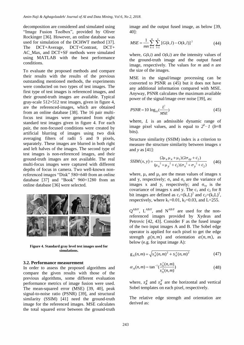
from an online database [38]. The 16 pair multi-
focus test images were generated from eight
standard test images given in figure 4. For each
pair, the non-focused conditions were created by
artificial blurring of images using two disk
averaging filters of radii 5 and 9 pixels,
separately. These images are blurred in both right
and left halves of the images. The second type of
test images is non-referenced images, and their
ground-truth images are not available. The real
multi-focus images were captured with different
depths of focus in camera. Two well-known non-
referencedimages“Disk”580×640fromanonline
database [37] and “Book” 960×1280 from an
online database [36] were selected.
3.2. Performance measurement
In order to assess the proposed algorithms and
compare the given results with those of the
previous algorithms, some different evaluation
performance metrics of image fusion were used.
The mean-squared error (MSE) [39, 40], peak
signal-to-noise ratio (PSNR) [39], and structural
similarity (SSIM) [41] need the ground-truth
image for the referenced images. MSE calculates
the total squared error between the ground-truth
image and the output fused image, as below [39,
40]:
2
1 1
1[ ( , ) ( , )]
m n
k l
MSE G k l O k lmn
(44)
where, G(k,l) and O(k,l) are the intensity values of
the ground-truth image and the output fused
image, respectively. The values for m and n are
the size of the images.
MSE in the signal/image processing can be
converted to PSNR as (45) but it does not have
any additional information compared with MSE.
Anyway, PSNR calculates the maximum available
power of the signal/image over noise [39], as:
2
10 ( )10 logL
MSEPSNR (45)
where, L is an admissible dynamic range of
image pixel values, and is equal to 2b−1 (b=8
bits).
Structure similarity (SSIM) index is a criterion to
measure the structure similarity between images x
and y as [41]:
2 2 2 2
1 2
1 2
(2 ) (2 )
( ) ( )( , )
x x xy
x y x y
cSSIM x y
c c
(46)
where, µx and µy are the mean values of images x
and y, respectively; σx andσy are the variance of
images x and y, respectively; and σxy is the
covariance of images x and y. The c1 and c2 for 8
bit images are defined as c1=(k1L)2 and c2=(k2L)
2,
respectively, where k1=0.01, k2=0.03, and L=255.
QAB/F
, LAB/F
, and NAB/F
are used for the non-
referenced images provided by Xydeas and
Petrovic [42, 43]. Consider F as the fused image
of the two input images A and B. The Sobel edge
operator is applied for each pixel to get the edge
strength and orientation as
below (e.g. for input image A):
2 2g ( , ) ( , ) ( , )yxA A An m s n m n ms (47)
1 ( , )( , ) tan ( )
( , )
y
AA x
A
s n mn m
s n m (48)
where, and
are the horizontal and vertical
Sobel templates on each pixel, respectively.
The relative edge strength and orientation are
derived as:
Figure 4. Standard gray level test images used for
simulations.
Amin-Naji & Aghagolzadeh/ Journal of AI and Data Mining, Vol 6, No 2, 2018.
244
,
, ,
,
,
,
,
F
n m A F
n m n mA
n mAF
n m A
n m
F
n m
gif g g
gG
gotherwise
g
(49)
/ 2
( , ) ( , )( , ) 1AF FA n m n m
A n m
(50)
Using (49) and (50), the edge strength and
orientation preservation values are derived as:
( ( , ) )( , )
1AF
g g
gAFg K G n m
Q n me
(51)
( ( , ) )( , )
1AF
AF
K A n mQ n m
e
(52)
The constants , , , , , and
determine the exact shape of the sigmoid
functions used to form the edge strength and
orientation preservation values. Thus the edge
information preservation is derived as:
( , ) ( , ) ( , )AF AF AFgQ n m Q n m Q n m (53)
where, 0 ( , ) 1AFQ n m . The zero value indicates
the complete loss of edge information, and the
value 1 indicates no loss of edge information in
the fusion process.
Finally, the total gradient information transferred
from the source images to the fused image
( /AB FQ ) is calculated as:
,/
,
, , , ,
, ,
n mAB F
n m
AF A BF Bn m n m n m n m
A Bn m n m
Q w Q w
Qw w
(54)
where, ,AFn mQ and ,
BFn mQ are weighted by
and
, respectively. The constant value L is
considered for [
] and
[ ]
.
The constant values used in this paper were taken
from [41] (L=1, , ,
, , , ).
LAB/F
is the fusion loss, which measures the
gradient information lost during the image fusion
process, and is calculated as below [43]:
/
,
,
,
, , , ,
, ,
[(1 ) (1 ) ]
AB F
n m
n m
n m
AF A BF Bn m n m n m n m
A Bn m n m
L
r Q w Q w
w w
(55)
where
, , , ,
,
1
0
F A F B
n m n m n m n m
n m
if g g or g gr
otherwise
(56)
NAB/F
is the fusion artefacts or noise [43]. NAB/F
measures the information that is not related to the
input images but is created as artefacts during the
image fusion process, and is calculated as:
,
,/
,
, ,
, ,
( )n m
n mAB F
n m
A Bn m n m
A Bn m n m
N w w
Nw w
(57)
where
,
, , , , ,2 &
0
n m
AF BF F A B
n m n m n m n m n m
N
Q Q if g g g
otherwise
(58)
In addition, we used the feature mutual
information (FMI) [44] as (59). The edge feature
of images was considered for information
representation in FMI.
FA FB
F A F B
ABF
I IFMI
H H H H
(59)
where, HA, HB, and HF are the information entropy
of the input images A, B, and the fused image,
respectively; and IFA and IFB are the amounts of
feature information that F contains about images
A and B, respectively.
These evaluation performance metrics (QAB/F
,
LAB/F
, NAB/F
, and FMI) were used for the non-
reference images, i.e. their ground-truth images
are not available.
3.3. Fusion result evaluation
Firstly, in order to demonstrate the advantages of
the proposed methods over the other ones, the
proposed methods and the previous ones were
applied on the 16 pairs of artificial multi-focus
images generated from the test images given in
figure 4. The average values for SSIM and MSE
for the proposed and other methods are listed in
table 1. The results obtained show that all the four
proposed methods give better results than the
other methods. The DCT+Eng_Corr method
shows the best results in these experiments, i.e.
the MSE and SSIM values for the DCT+Eng_Corr

Amin-Naji & Aghagolzadeh/ Journal of AI and Data Mining, Vol 6, No 2, 2018.
245
method are 1.9594 and 0.9950, respectively,
which are the lowest MSE and highest SSIM
values among the other values of the other
methods.
Secondly, the proposed methods and the other
ones are evaluated by real multi-focus images
with different depths of focus in camera. The
methods were applied on the various sizes of
images like “Disk” 580×640 and “Book”
960×1280, so evaluation results for the
performance metrics (QAB/F
, LAB/F
, NAB/F
, and
FMI) were obtained and listed in table 2. The non-
reference multi-focus image fusion metrics values
for the realistic images emphasize the advantages
of the proposed methods over the other ones. The
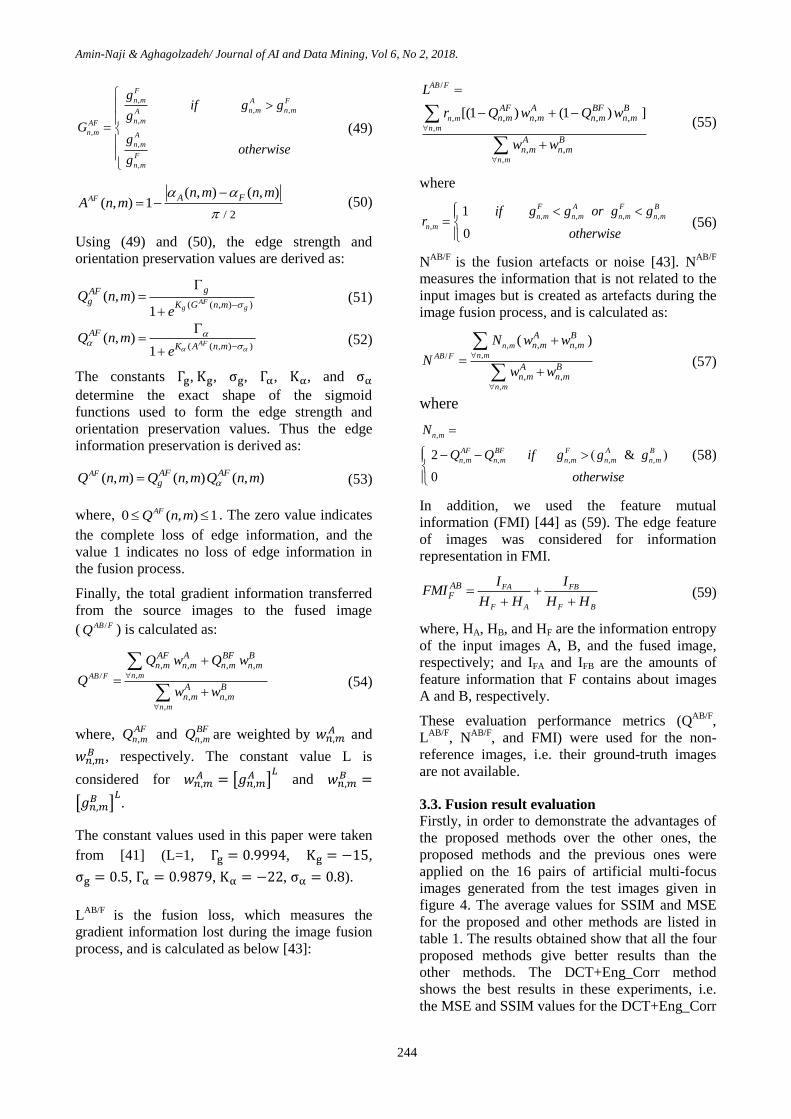
output fused images of the proposed methods and
the „„Book‟‟ source images focusing on the left
and the right are shown in figure 5. Beside this,
the magnified output images of the proposed and
previous methods are shown in figure 5. There are
some undesirable side-effects like blurring in the
DCT+Average and DCT+Contrast methods.
However, the ringing artefacts in wavelet-based
methods, and blocking effects/unsuitable block
selection in the DCT+Variance, DCT+AC_Max,
and DCT+SF methods could be concluded from
the output image results. All the proposed
methods could enhance the quality of output fused
image and reduce unsuitable block selection
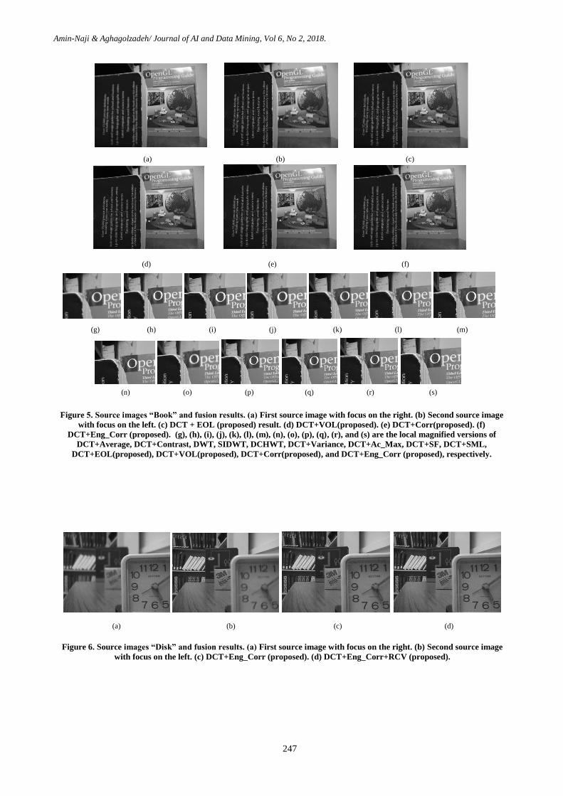
significantly.Similarly,the„„Disk‟‟sourcemulti-
focus images and the results of the proposed
methods (DCT+Eng_Corr and
DCT+Eng_Corr+RCV) are shown in figure 6.
However, the RCV process and the CV process,
as the post-processing, are applied on the DCT-
basedmethods for fusion of “Book” images and
16 pair multi-focus images that were generated.
The evaluation performance metrics of CV and
RCV are listed in table 3. The results obtained
showed that although CV enhanced the quality of
the output fused image in most cases, the ability
of RCV was more than CV in enhancing the
quality of output fused image. In addition, RCV
could prevent the unsuitable block selection
significantly and remove the blocking effects
completely in the output fused image. The visual
comparisonofCVandRCVofthe“Book”image,
shown in figure 7 demonstrate this claim.
In another experiment, the proposed methods and
the pervious ones were conducted on the “Lena”
and “Pepper” multi-focus images. The non-
focused conditions of these multi-focus images
were created by artificial blurring of images using
a disk averaging filter of radius 9 pixel. The
PSNR values for the fused output image of
different methods are recorded in table 4. It is
understandable that the PSNR values for the
results of the latest method for“Lena” is infinite
(∞). Focusedblockrecognitionof“Lena”iseasy
because of the inherent high local correlation
among pixel values and high contrast between
adjacent areas, whereas the focused block
recognition of “Pepper” is harder than “Lena”.
Thus we conducted experiments on“Pepper”as a
harder quality test in order to compare the
methods in fair conditions. All proposed methods
have better results over the previous ones. The
ground-truth image, multi-focus images of
“Pepper”,difference imagesbetween the ground-
truth images, fused output images of the proposed
methods, and other methods are depicted in figure
7. DCT+VOL+RCV and DCT+Eng_Corr+RCV
have the best results in the PSNR values, and have
less image differences in table 4 and figure 7,
respectively.
In this paper, four new multi-focus image fusion
methods are introduced. All the proposed methods
have significant improvements in the quality of
the output fused images. In fact, all the DCT-
based fusion methods for JPEG image are less
time-consuming and suitable for implementation
in real-time applications. However, it is important
that which one is faster in order to implement in
the real-time applications. We conducted an
average run-time comparison for our proposed
methods in table 5. Our proposed algorithms were
performed using the MATLAB 2016b software
with an 8 GB RAM and Intel core i7-7500 CPU
processor @ 2.7GHz & 2.9 GHz. According to
table 5, DCT+Vol has the best run-time (0.110408
s) for fusion of 512×512 multi-focus images, and
next, DCT+Eol, DCT+Corr, and DCT+Eng+Corr
have 0.124598, 0.160410, and 0.173938 s run
times, respectively. DCT+VOL has a better image
quality and faster algorithm run-time than
DCT+Corr & DCT+EOL. According to tables 1,
2, 3, and 4, the best quality result is for
DCT+Eng_Corr, and after that is for DCT+VOL.
Thus we can conclude that DCT+Eng_Corr is a
better choice if the powerful hardware is
available, and time-consumption has little
importance. On the other side, DCT+VOL is a
better choice if there is a critical need for time and
energy-consumption. Anyway, all proposed
methods have significant improvement in quality
of the output fused images, and are appropriate for
real-time applications due to implantation in the
DCT domain.

Amin-Naji & Aghagolzadeh/ Journal of AI and Data Mining, Vol 6, No 2, 2018.
246
4. Conclusions
In this paper, four new multi-focus image fusion
methods were introduced completely in the DCT
domain. By proposing an algorithm for
convolving a mask on the 8×8 block directly in
the DCT domain, we could calculate the image
Laplacian and image low-pass filtering in DCT
domain. Thus two powerful Laplacian-based
focus measurements, VOL and EOL were
implemented in the DCT domain. Two other
powerful DCT focus measurements, DCT+Corr
and DCT+Eng_Corr, were introduced. These
methods measure the occurring changes in passing
image blocks through the low-pass filter in the
DCT domain. In addition, we substituted CV post-
processing with RCV. This replacement improved
the quality of the output fused image significantly
and prevents unsuitable block selection and
blocking effects in the output fused image. We
conducted a lot of experiments on various types of
multi-focus images. The accuracy of the proposed
methods is assessed by applying the proposed
algorithms and other well-known methods on the
several referenced images and non-referenced
images. However, evaluation of different methods
was done using various evaluation performance
metrics. The results obtained show the advantages
of the proposed algorithms over some precious
and the state of art algorithms in terms of quality
of output image. In addition, due to a simple
implementation of the proposed algorithms in the
DCT domain, they are appropriate for use in real-
time applications.
Table 1. MSE and SSIM comparison of various image
fusion methods on reference images.
Methods
Average values for 16 pairs
images created from image
shown in Fig. 4
MSE SSIM
DCT+Average [28] 65.1125 0.9164
DCT+Contrast [28] 23.0788 0.9647
DWT [23] 19.2411 0.9619
SIDWT [24] 15.5693 0.9641
DCHWT [25] 4.7756 0.9902
DCT+Variance [27] 17.2293 0.9720
DCT+AC_Max [29] 4.1520 0.9917
DCT+SF [30] 5.6848 0.9896
DCT+SML [31] 9.8444 0.9828
DCT+ EOL (proposed)
2.5487 0.9944
DCT+VOL (proposed) 2.5486 0.9944
DCT+Corr (proposed) 5.2722 0.9921
DCT+Eng_Corr (proposed) 1.9594 0.9950
Table 2. QAB/F, LAB/F, NAB/F, and FMI comparison of various image fusion methods on non-referenced images.
Methods
“BOOK”
“DISK”
QAB/F LAB/F NAB/F FMI QAB/F LAB/F NAB/F FMI
DCT+Average [28] 0.4985 0.5002 0.0025 0.9075 0.5187 0.4782 0.0063 0.9013
DCT+Contrast [28] 0.6470 0.2384 0.3736 0.9074 0.6212 0.2554 0.3629 0.8981
DWT [23] 0.6621 0.2294 0.3569 0.9117 0.6302 0.2552 0.3362 0.9039
SIDWT [24] 0.6932 0.2637 0.1279 0.9122 0.6694 0.2764 0.1564 0.9049
DCHWT [25] 0.6684 0.3014 0.0705 0.9123 0.6529 0.3140 0.0789 0.9075
DCT+Variance [27] 0.7210 0.2660 0.0277 0.9135 0.7165 0.2612 0.0478 0.9070
DCT+AC_Max [29] 0.7081 0.2781 0.0294 0.9136 0.6763 0.2910 0.0696 0.9057
DCT+SF [30] 0.7151 0.2757 0.0197 0.9148 0.7213 0.2600 0.0415 0.9086
DCT+SML [31] 0.6960 0.2928 0.0241 0.9147 0.6774 0.3074 0.0324 0.9080
DCT+ EOL (proposed)
0.7283 0.2620 0.0206 0.9153 0.7280 0.2522 0.0425 0.9094
DCT+VOL (proposed) 0.7284 0.2619 0.0207 0.9153 0.7285 0.2519 0.0421 0.9094
DCT+Corr (proposed) 0.7281 0.2622 0.0207 0.9153 0.7246 0.2541 0.0456 0.9087
DCT+Eng_Corr (proposed) 0.7284 0.2622 0.0202 0.9155 0.7288 0.2530 0.0391 0.9094
Amin-Naji & Aghagolzadeh/ Journal of AI and Data Mining, Vol 6, No 2, 2018.
247
(a) (b) (c)
(d) (e) (f)
(g) (h) (i) (j) (k) (l) (m)
(n) (o) (p) (q) (r) (s)
Figure 5. Source images “Book” and fusion results. (a) First source image with focus on the right. (b) Second source image
with focus on the left. (c) DCT + EOL (proposed) result. (d) DCT+VOL(proposed). (e) DCT+Corr(proposed). (f)
DCT+Eng_Corr (proposed). (g), (h), (i), (j), (k), (l), (m), (n), (o), (p), (q), (r), and (s) are the local magnified versions of
DCT+Average, DCT+Contrast, DWT, SIDWT, DCHWT, DCT+Variance, DCT+Ac_Max, DCT+SF, DCT+SML,
DCT+EOL(proposed), DCT+VOL(proposed), DCT+Corr(proposed), and DCT+Eng_Corr (proposed), respectively.
(a) (b) (c) (d)
Figure 6. Source images “Disk” and fusion results. (a) First source image with focus on the right. (b) Second source image
with focus on the left. (c) DCT+Eng_Corr (proposed). (d) DCT+Eng_Corr+RCV (proposed).

Amin-Naji & Aghagolzadeh/ Journal of AI and Data Mining, Vol 6, No 2, 2018.
248
Table 3. Comparison between CV and RCV post-processing algorithms.
Methods
Average values for 16 pair
image created from image
shown in Fig. 4
“BOOK”
MSE SSIM QAB/F LAB/F NAB/F FMI
DCT+Variance+CV [27] 2.8536 0.9961
0.7222 0.2753 0.0056 0.9151
DCT+AC_Max+CV [29] 1.3784 0.9972
0.7180 0.2778 0.0095 0.9157
DCT+SF+CV [30] 2.1456 0.9968
0.7169 0.2796 0.0080 0.9159
DCT+SML+CV [31] 2.3901 0.9959
0.7187 0.2780 0.0072 0.9163
DCT+ EOL+CV (proposed)
1.0720 0.9976
0.7271 0.2714 0.0036 0.9162
DCT+VOL +CV(proposed) 1.0735 0.9976
0.7278 0.2708 0.0033 0.9163
DCT+Corr+CV (proposed) 1.7408 0.9974
0.7280 0.2706 0.0033 0.9163
DCT+Eng_Corr+CV (proposed) 0.8329 0.9979
0.7285 0.2701 0.0030 0.9163
DCT+VOL+RCV (proposed) 0.8491 0.9978
0.7290 0.2695 0.0024 0.9164
DCT+Eng_Corr+RCV (proposed) 0.6623 0.9980
0.7301 0.2690 0.0019 0.9165
(a) (b) (c) (d) (e) (f)
(g) (h) (i) (j) (k) (l)
(m) (n) (o) (p) (q) (r)
Figure 7. Source images and multi-focus images of “Pepper”, and difference images between ground-truth image and fused
output images of proposed methods and other methods. (a) Ground-truth image. (b) First source image with focus on the right.
(c) Second source image with focus on the left. (d) DCT+Average. (e) DCT+Contrast. (f) DWT. (g) SIDWT. (h) DCHWT. (i)
DCT+Variance+CV. (j) DCT+Ac_Max+CV. (k) DCT+SF+CV. (l) DCT+SML+CV. (m) DCT+EOL+CV (Proposed). (n)
DCT+VOL+CV (Proposed). (o) DCT+Corr+CV (Proposed). (p) DCT+Eng_Corr+CV (Proposed). (q) DCT+VOL+RCV
(Proposed). (r) DCT+Eng_Corr+RCV (Proposed).

Amin-Naji & Aghagolzadeh/ Journal of AI and Data Mining, Vol 6, No 2, 2018.
249
References
[1] Drajic, D. & Cvejic, N. (2007). Adaptive fusion of
multimodal surveillance image sequences in visual
sensor networks. IEEE Transactions on Consumer
Electronics, vol. 53, no. 4, pp. 1456-1462.
[2] Wu, W., Yang, X., Pang, Y., Peng, J. & Jeon, G.
(2013). A multifocus image fusion method by using
hidden Markov model. Optics Communication, vol.
287, January, pp. 63-72.
[3] Kumar, B., Swamy, M. & Ahmad, M. O. (2013).
Multiresolution DCT decomposition for multifocus
image fusion. In 26th Annual IEEE Canadian
Conference on Electrical and Computer Engineering
(CCECE), pp. 1-4.
[4] Haghighat, M. B. A, Aghagolzadeh, A. &
Seyedarabi, H. (2010). Real-time fusion of multi-focus
images for visual sensor networks. In 6th Iranian
Machine Vision and Image Processing (MVIP), pp. 1-
6.
[5] Naji, M. A., & Aghagolzadeh, A. (2015). A new
multi-focus image fusion technique based on variance
in DCT domain. In 2nd International Conference on
Knowledge-Based Engineering and Innovation (KBEI),
pp. 478-484.
[6] Castanedo, F., García, J., Patricio, M., & Molina,
J.M. (2008). Analysis of distributed fusion alternatives
in coordinated vision agents. In 11th International
Conference on Information Fusion, pp. 1-6.
[7] Kazemi, V., Seyedarabi, H. & Aghagolzadeh, A.
(2014). Multifocus image fusion based on compressive
sensing for visual sensor networks. In 22nd Iranian
Conference on Electrical Engineering (ICEE), pp.
1668-1672.
[8] Soro, S., & Heinzelman, W. (2009). A Survey of
Visual Sensor Networks. Advances in Multimedia. vol.
2009, Article ID 640386, 21 pages, May.
[9] Huang, W. & Jing, Z. (2007). Evaluation of focus
measures in multi-focus image fusion. Pattern
Recognition Letters, vol. 28, no. 4, pp. 493-500.
[10] Li, S., Kwok, J. T., & Wang, Y. (2001).
Combination of images with diverse focuses using the
spatial frequency, Information fusion, vol. 2, no. 3, pp.
169-176.
[11] Li, S., & Yang, B. (2008). Multifocus Image
Fusion Using Region Segmentation and Spatial
Frequency. Image and Vision Computing, vol. 26, no.
7, pp. 971-979.
[12] Hongmei, W., Cong, N., Yanjun, L., & Lihua, C.
(2011). A Novel Fusion Algorithm for Multi-focus
Image. International Conference on Applied
Informatics and Communication (ICAIC), pp. 641-647.
[13] Mahajan, S., & Singh, A. (2014). A Comparative
Analysis of Different Image Fusion Techniques. IPASJ
International Journal of Computer Science (IIJCS), vol.
2, no. 1, pp. 634-642.
[14] Pertuz, S., Puig, S. D., & Garcia, M. A. (2013).
Analysis of focus measure operators for shape-from-
focus. Pattern Recognition. Vol. 46, no. 5, pp.1415-
1432.
[15] Kaur, P., & Kaur, M. (2015). A Comparative
Study of Various Digital Image Fusion Techniques: A
Review. International Journal of Computer
Applications, vol. 114, no. 4.
[16] Zhao, H., Li, Q., & Feng, H. (2008). Multi-focus
color image fusion in the HSI space using the sum-
modified-Laplacian and a coarse edge map. Image and
Vision Computing, vol. 26, no.9, pp. 1285-1295.
[17] Zaveri, T., Zaveri, M., Shah, V., & Patel, N.
(2009). A Novel Region Based Multifocus Image
Fusion Method. Proceeding of IEEE International
Conference on Digital Image Processing (ICDIP), pp.
50-54.
[18] Eltoukhy, H. A., & Kavusi, S. (2003).
Computationally efficient algorithm for multifocus
Table 4. PSNR comparison between multi-focus image
fusion methods on “Lena” and “House” images.
Methods
PSNR (dB)
“Lena” “Pepper”
DCT+Average [28] 29.6283 29.6283
DCT+Contrast [28] 32.3775 33.3672
DWT [23] 34.8943 33.7156
SIDWT [24] 36.0411 34.6095
DCHWT [25] 40.8483 42.9835
DCT+Variance+CV [27] 34.3470 33.5931
DCT+AC_Max+CV [29] ∞ 40.8329
DCT+SF+CV [30] 39.5646 40.4470
DCT+SML+CV [31] ∞ 35.1566
DCT+ EOL+CV (proposed)
∞ 44.0011
DCT+VOL+CV (proposed) ∞ 44.0011
DCT+Corr+CV (proposed) ∞ 40.3896
DCT+Eng_Corr+CV (proposed) ∞ 48.6852
DCT+VOL+RCV (proposed) ∞ 48.4816
DCT+Eng_Corr+RCV (proposed) ∞ 54.3365
Table 5. Average Run-Time comparison between four
proposed 512×512 multi-focus image fusion methods.
Methods
Time (s)
DCT+ EOL (proposed)
0.124598
DCT+VOL (proposed) 0.110408
DCT+Corr (proposed) 0.160410
DCT+Eng_Corr (proposed) 0.173938
Amin-Naji & Aghagolzadeh/ Journal of AI and Data Mining, Vol 6, No 2, 2018.
250
image reconstruction. Proceedings SPIE Electronic
Imaging, vol. 5017, pp. 332–341.
[19] Zhan, K., Teng, J., Li, Q., & Shi, J. (2015). A
Novel Explicit Multi-focus Image Fusion Method.
Journal of Information Hiding and Multimedia Signal
Processing, vol. 6, no. 3, pp. 600-612.
[20] Burt P. J., & Adelson, E. H. (1983). The Laplacian
pyramid as a compact image code. IEEE Transactions
Communications. Vol. 31, no. 4, pp. 532-540.
[21] Petrovic V. S., & Xydeas, C. S. (2004). Gradient-
based multiresolution image fusion. IEEE Transactions
Image Processing. vol. 13, no. 2, pp. 228-237.
[22] De, I., & Chanda, B. (2006). A simple and
efficient algorithm for multifocus image fusion using
morphological wavelets. Signal Processing. vol. 86, no.
5, pp. 924-936.
[23] Li, H., Manjunath, B., & Mitra, S. K. (1995).
Multisensor image fusion using the wavelet transform.
Graphical models and image processing. vol. 57, no.3,
pp. 235-245.
[24] Rockinger, O. (1997). Image sequence fusion
using a shift-invariant wavelet transform. Proceedings
of the IEEE International Conference on Image
Processing, pp. 288–291.
[25] Kumar, B. K. S. (2013). Multifocus and
multispectral image fusion based on pixel significance
using discrete cosine harmonic wavelet transform.
Signal, Image and Video Processing, vol. 7, no. 6,
pp.1125-1143.
[26] Tang, J., Peli, E., & Acton, S. (2003). Image
enhancement using a contrast measure in the
compressed domain. IEEE Signal Processing Letters,
vol. 10, no.10, pp. 289-292.
[27] Haghighat, M. B. A, Aghagolzadeh, A., &
Seyedarabi, H. (2011). Multi-focus image fusion for
visual sensor networks in DCT domain. Computers &
Electrical Engineering, vol. 37, no. 5, pp. 789-797.
[28] Tang, J. (2004). A contrast based image fusion
technique in the DCT domain. Digital Signal
Processing, vol. 14, no. 3, pp. 218-226.
[29] Phamila Y. A. V., & Amutha, R. (2014). Discrete
Cosine Transform based fusion of multi-focus images
for visual sensor networks. Signal Processing, vol. 95,
pp. 161-170.
[30] Cao, L., Jin, L., Tao, H., Li, G., Zhuang, Z., &
Zhang, Y. (2015). Multi-focus image fusion based on
spatial frequency in discrete cosine transform domain.
IEEE Signal Processing Letters, vol. 22, no. 2, pp. 220-
224.
[31] Abdollahzadeh, M., Malekzadeh, M., &
Seyedarabi, H. (2016). Multi-focus image fusion for
visual sensor networks. In 24th Iranian Conference on
Electrical Engineering (ICEE), pp. 1673-1677.
[32] Amin-Naji, M., & Aghagolzadeh, A. (2016).
Block DCT filtering using vector processing. In 2016
1st International Conference on New Research
Achievements in Electrical and Computer Engineering
(ICNRAECE), pp. 722-727.
[33] Naji, M. A., & Aghagolzadeh, A. (2015). Multi-
focus image fusion in DCT domain based on
correlation coefficient. In 2nd International Conference
on Knowledge-Based Engineering and Innovation
(KBEI), pp. 632-639.
[34] Amin-Naji, M., & Aghagolzadeh, A. (2016).
Multi-focus image fusion using VOL and EOL in DCT
domain. In 2016 1st International Conference on New
Research Achievements in Electrical and Computer
Engineering (ICNRAECE), pp. 728-733.
[35] Haghighat, M. B. A. Multi-Focus Image Fusion in
DCT Domain, (2016), Available:
https://github.com/mhaghighat/dctVarFusion
[36] Rockinger, O. image fusion toolbox, (1999).
Available: http://www.metapix.de/toolbox.htm
[37] Kumar, B. K. S., Multifocus and multispectral
image fusion based on pixel significance using dchwt,
(2013), Available:
http://www.mathworks.com/matlabcentral/fileexchang
e/43051-multifocus-and-multispectral-image-fusion-
based-on-pixel-significance-using-dchwt
[38] Image processing place, Available:
http://www.imageprocessingplace.com/root_files_V3/i
mage_databases.htm
[39] Wang, Z., & Bovik, A. (2009). Mean squared
error: Love it or leave it? A new look at Signal Fidelity
Measures. IEEE Signal Processing Magazine, vol. 26,
no. 1, pp. 98-117.
[40] Esmilizaini, A. M, Latif, A. M., & Loghmani, Gh.
B. (2017). Tuning Shape Parameter of Radial Basis
Functions in Zooming Images using Genetic
Algorithm. Journal of AI & Data Mining, Articles in
Press.
[41] Wang, Z., Bovik, A. C., Sheikh, H. R., &
Simoncelli, E. P. (2004). Image quality assessment:
from error visibility to structural similarity. IEEE
Transactions on Image Processing, vol. 13, no.4, pp.
600-612.
[42] Xydeas, C., & Petrovic, V. (2000). Objective
image fusion performance measure. Electronics
Letters, vol. 36, no.4, pp. 308-309.
[43] Petrovic, V., & Xydeas, C. (2005). Objective
image fusion performance characterization. In Tenth
IEEE International Conference on Computer Vision
(ICCV), pp. 1866-1871.
[44] Haghighat, M. B. A, Aghagolzadeh, A., &
Seyedarabi, H. (2011). A non-reference image fusion
metric based on mutual information of image features.
Computers & Electrical Engineering, vol. 37, no. 5, pp.
744-756.