Embed Size (px)
Citation preview


Multi-CarrierDigital Communications
Theory and Applications of OFDM

Information Technology: Transmission, Processing, and Storage
Series Editor: Jack Keil WolfUniversity of California at San DiegoLa Jolla, California
Editorial Board: James E. MazoBell Laboratories, Lucent TechnologiesMurray Hill, New Jersey
John ProakisNortheastern UniversityBoston, Massachusetts
William H. TranterVirginia Polytechnic Institute and State UniversityBlacksburg, Virginia
Multi-Carrier Digital Communications: Theory and Applications of OFDMAhmad R. S. Bahai and Burton R. Saltzberg
Principles of Digital Transmission: With Wireless ApplicationsSergio Benedetto and Ezio Biglieri
Simulation of Communication Systems, 2nd Edition: Methodology, Modeling,and TechniquesMichel C. Jeruchim, Philip Balaban, and K. Sam Shanmugan
A Continuation Order Plan is available for this series. A continuation order will bring delivery of each new volumeimmediately upon publication. Volumes are billed only upon actual shipment. For further information please contactthe publisher.
Multi-CarrierDigital Communications
Theory and Applications of OFDM
Ahmad R. S. Bahai andBurton R. Saltzberg
Algorex, Inc.Iselin, New Jersey
Kluwer Academic PublishersNew York, Boston, Dordrecht, London, Moscow
eBook ISBN: 0-306-46974-XPrint ISBN: 0-306-46296-6
©2002 Kluwer Academic PublishersNew York, Boston, Dordrecht, London, Moscow
Print ©1999 Kluwer Academic / Plenum PublishersNew York
All rights reserved
No part of this eBook may be reproduced or transmitted in any form or by any means, electronic,mechanical, recording, or otherwise, without written consent from the Publisher
Created in the United States of America
Visit Kluwer Online at: http://kluweronline.comand Kluwer's eBookstore at: http://ebooks.kluweronline.com
Preface
Multi-carrier modulation, in particular Orthogonal Frequency Division
Multiplexing (OFDM), has been successfully applied to a wide variety ofdigital communications applications over the past several years. AlthoughOFDM has been chosen as the physical layer standard for a diversity ofimportant systems, the theory, algorithms, and implementation techniquesremain subjects of current interest. This is clear from the high volume ofpapers appearing in technical journals and conferences.
This book is intended to be a concise summary of the present state of theart of the theory and practice of OFDM technology. The authors believe that
the time is ripe for such a treatment. Particularly based on one of the author'slong experience in development of wireless systems, and the other's inwireline systems, we have attempted to present a unified presentation of
OFDM performance and implementation over a wide variety of channels. Itis hoped that this will prove valuable both to developers of such systems andto researchers and graduate students involved in analysis of digitalcommunications.
In the interest of brevity, we have minimized treatment of more generalcommunication issues. There exist many excellent texts on communication
v
vi Preface
theory and technology. Only brief summaries of topics not specific to multi-carrier modulation are presented in this book where essential.
We begin with a historical overview of multi-carrier communications,wherein its advantages for transmission over highly dispersive channels havelong been recognized, particularly before the development of equalizationtechniques. We then focus on the bandwidth efficient technology of OFDM,in particular the digital signal processing techniques that have made themodulation format practical. Several chapters describe and analyze the sub-systems of an OFDM implementation, such as synchronization, equalization,and coding. Analysis of performance over channels with variousimpairments is presented. The chapter on effects of clipping presents resultsof the authors that have not yet been published elsewhere.
The book concludes with descriptions of three very important anddiverse applications of OFDM that have been standardized and are nowbeing deployed. ADSL provides access to digital services at several Mb/sover the ordinary wire-pair connection between customers and the localtelephone company central office. Digital Broadcasting enables the radioreception of high quality digitized sound and video. A unique configurationthat is enabled by OFDM is the simultaneous transmission of identicalsignals by geographically dispersed transmitters. Finally, the newdevelopment of wireless LANs for multi-Mb/s communications is presented.Each of these successful applications required the development of new
fundamental technology.
Multi-carrier modulation continues to evolve rapidly. It is hoped that thisbook will remain a valuable summary of the technology, providing anunderstanding of new advances as well as the present core technology.
We acknowledge the extensive review and many valuable suggestions ofProfessor Kenji Kohiyama, our former colleagues at AT&T BellLaboratories and colleagues at Algorex. Gail Bryson performed the verydifficult task of editing and assembling this text. The continuing support of

Preface vii
Kambiz Homayounfar was essential to its completion. Last, but by no means
least, we are thankful to our families for their support and patience.
Contents
CHAPTER 1 INTRODUCTION TO DIGITAL COMMUNICATIONS ............................2
1.11.2
BACKGROUND ..................................................................................................................EVOLUTION OF OFDM ..............................................................................................................
27
CHAPTER 2 SYSTEM ARCHITECTURE .................................................................................17
2.12.22.32.42.52.6
MULTI-CARRIER SYSTEM FUNDAMENTALS .........................................................................DFT............................................................................................................................PARTIAL FFT..............................................................................................................CYCLIC EXTENSION .....................................................................................................CHANNEL ESTIMATION ....................................................................................................APPENDIX — MATHEMATICAL MODELLING OF OFDM FOR TIME-VARYING
1720252729
32RANDOM CHANNEL .................................................................................................................
CHAPTER 3 PERFORMANCE OVER TIME-INVARIANT CHANNELS ..................41
3.13.23.33.4
TIME-INVARIANT NON-FLAT CHANNEL WITH COLORED NOISE ........................................ERROR PROBABILITY ........................................................................................................BIT ALLOCATION ...........................................................................................................BIT AND POWER ALLOCATION ALGORITHMS FOR FIXED BIT RATE .....................................
41
424653
CHAPTER 4 CLIPPING IN MULTI-CARRIER SYSTEMS ..........................................57
4.14.24.34.4
INTRODUCTION ..............................................................................................................POWER AMPLIFIER NON-LINEARITY ................................................................................BER ANALYSIS ............................................................................................................BANDWIDTH REGROWTH ..........................................................................................
57596376
ix

x Contents
CHAPTER 5 SYNCHRONIZATION................................................................................83
5.15.25.35.45.5
TIMING AND FREQUENCY OFFSET IN OFDM ...........................................................SYNCHRONIZATION AND SYSTEM ARCHITECTURE .................................................................TIMING AND FRAME SYNCHRONIZATION ....................................................................FREQUENCY OFFSET ESTIMATION ....................................................................................PHASE NOISE ...........................................................................................................
8388899193
CHAPTER 6 EQUALIZATION .......................................................................................103
6.16.26.36.46.56.6
INTRODUCTION .............................................................................................................TIME DOMAIN EQUALIZATION .........................................................................................EQUALIZATION IN DMT ....................................................................................................FREQUENCY DOMAIN EQUALIZATION ..............................................................................ECHO CANCELLATION ....................................................................................................APPENDIX — JOINT INNOVATION REPRESENTATION OF ARMA MODELS ................................
103104109116120127
CHAPTER 7 CHANNEL CODING .................................................................................135
7.17.27.37.47.57.6
NEED FOR CODING .....................................................................................................................BLOCK CODING IN OFDM .........................................................................................CONVOLUTIONAL ENCODING .........................................................................................CONCATENATED CODING ............................................................................................TRELLIS CODING IN OFDM .................................................................................TURBO CODING IN OFDM ..........................................................................................
135136142147148153
CHAPTER 8 ADSL............................................................................................................159
8.18.28.3
WIRED ACCESS TO HIGH RATE DIGITAL SERVICES .......................................................PROPERTIES OF THE WIRE-PAIR CHANNEL ......................................................................ADSL SYSTEMS ...............................................................................................................
159160170
CHAPTER 9 WIRELESS LAN ........................................................................................175
9.19.29.39.4
INTRODUCTION ..............................................................................................................PHYSICAL LAYER TECHNIQUES FOR WIRELESS LAN ..........................................................OFDM FOR WIRELESS LAN .....................................................................................RECEIVER STRUCTURE .................................................................................................
175181182187
Contents xi
CHAPTER 10 DIGITAL BROADCASTING..........................................................................191
10.110.210.310.4
BROADCASTING OF DIGITAL AUDIO SIGNALS .................................................................SIGNAL FORMAT ...........................................................................................................OTHER DIGITAL BROADCASTING SYSTEMS .......................................................................DIGITAL VIDEO BROADCASTING ..................................................................................
191194197198
CHAPTER 11 FUTURE TRENDS....................................................................................203
11.111.211.311.411.5
COMPARISON WITH SINGLE CARRIER MODULATION ...........................................................MITIGATION OF CLIPPING EFFECTS ..........................................................................OVERLAPPED TRANSFORMS ................................................................................COMBINED CDMA AND OFDM ..............................................................................ADVANCES IN IMPLEMENTATION ..............................................................................
INDEX..................................................................................................................................217
203205206210213
Multi-CarrierDigital Communications
Theory and Applications of OFDM
Chapter 1 Introduction to DigitalCommunications
1.1 Background
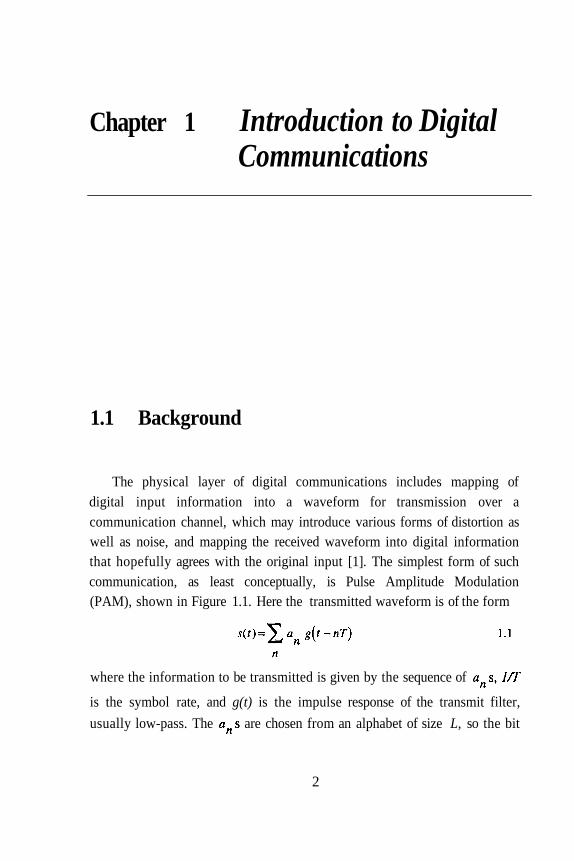
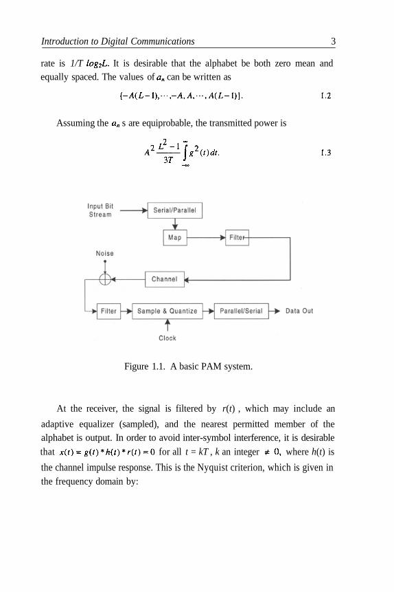
The physical layer of digital communications includes mapping ofdigital input information into a waveform for transmission over acommunication channel, which may introduce various forms of distortion aswell as noise, and mapping the received waveform into digital informationthat hopefully agrees with the original input [1]. The simplest form of suchcommunication, as least conceptually, is Pulse Amplitude Modulation(PAM), shown in Figure 1.1. Here the transmitted waveform is of the form
where the information to be transmitted is given by the sequence of
is the symbol rate, and g(t) is the impulse response of the transmit filter,
usually low-pass. The are chosen from an alphabet of size L, so the bit
2
Introduction to Digital Communications 3
rate is 1/T It is desirable that the alphabet be both zero mean andequally spaced. The values of can be written as
Assuming the s are equiprobable, the transmitted power is
Figure 1.1. A basic PAM system.
At the receiver, the signal is filtered by r(t) , which may include an
adaptive equalizer (sampled), and the nearest permitted member of thealphabet is output. In order to avoid inter-symbol interference, it is desirable
that for all t = kT , k an integer where h(t) is
the channel impulse response. This is the Nyquist criterion, which is given inthe frequency domain by:
4 Introduction to Digital Communications
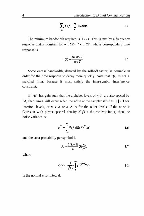
The minimum bandwidth required is 1 / 2T. This is met by a frequencyresponse that is constant for whose corresponding time
response is
Some excess bandwidth, denoted by the roll-off factor, is desirable inorder for the time response to decay more quickly. Note that r(t) is not a
matched filter, because it must satisfy the inter-symbol interferenceconstraint.
If r(t) has gain such that the alphabet levels of x(0) are also spaced by
2A, then errors will occur when the noise at the sampler satisfies for
interior levels, or or for the outer levels. If the noise isGaussian with power spectral density N( f ) at the receiver input, then thenoise variance is:
and the error probability per symbol is
where
is the normal error integral.
Introduction to Digital Communications 5
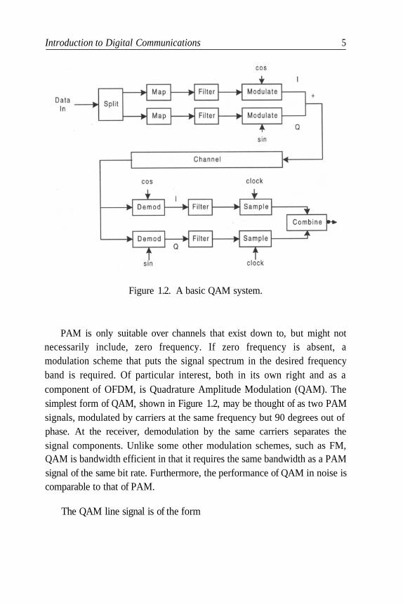
Figure 1.2. A basic QAM system.
PAM is only suitable over channels that exist down to, but might notnecessarily include, zero frequency. If zero frequency is absent, amodulation scheme that puts the signal spectrum in the desired frequencyband is required. Of particular interest, both in its own right and as acomponent of OFDM, is Quadrature Amplitude Modulation (QAM). Thesimplest form of QAM, shown in Figure 1.2, may be thought of as two PAMsignals, modulated by carriers at the same frequency but 90 degrees out ofphase. At the receiver, demodulation by the same carriers separates thesignal components. Unlike some other modulation schemes, such as FM,QAM is bandwidth efficient in that it requires the same bandwidth as a PAMsignal of the same bit rate. Furthermore, the performance of QAM in noise iscomparable to that of PAM.
The QAM line signal is of the form
6 Introduction to Digital Communications
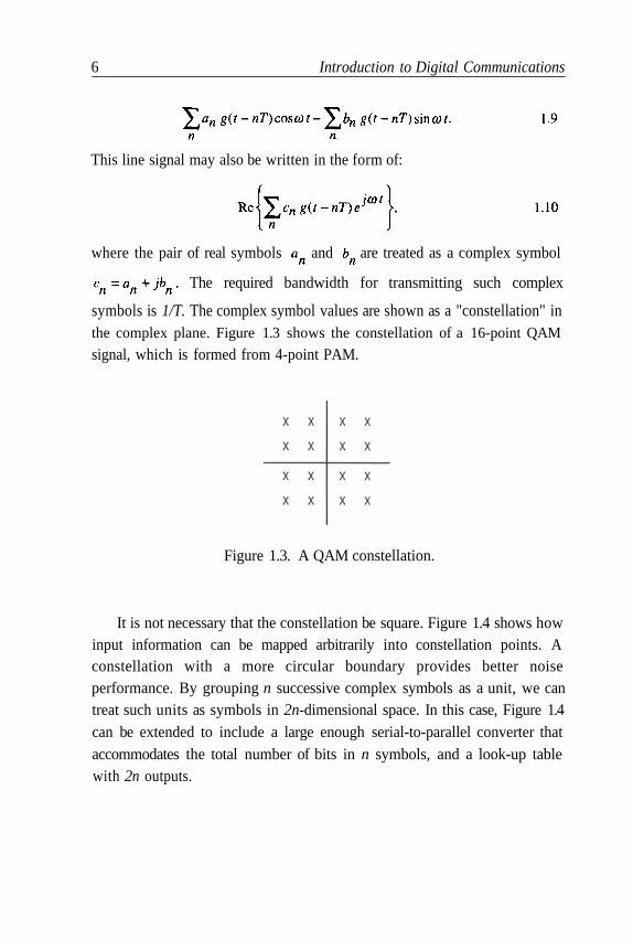
This line signal may also be written in the form of:
where the pair of real symbols and are treated as a complex symbol
The required bandwidth for transmitting such complex
symbols is 1/T. The complex symbol values are shown as a "constellation" inthe complex plane. Figure 1.3 shows the constellation of a 16-point QAM
signal, which is formed from 4-point PAM.
Figure 1.3. A QAM constellation.
It is not necessary that the constellation be square. Figure 1.4 shows howinput information can be mapped arbitrarily into constellation points. Aconstellation with a more circular boundary provides better noiseperformance. By grouping n successive complex symbols as a unit, we cantreat such units as symbols in 2n-dimensional space. In this case, Figure 1.4can be extended to include a large enough serial-to-parallel converter thataccommodates the total number of bits in n symbols, and a look-up tablewith 2n outputs.

Introduction to Digital Communications 7
Figure 1.4. General form of QAM generation.
1.2 Evolution of OFDM
The use of Frequency Division Multiplexing (FDM) goes back over acentury, where more than one low rate signal, such as telegraph, was carriedover a relatively wide bandwidth channel using a separate carrier frequency
for each signal. To facilitate separation of the signals at the receiver, thecarrier frequencies were spaced sufficiently far apart so that the signal
spectra did not overlap. Empty spectral regions between the signals assuredthat they could be separated with readily realizable filters. The resultingspectral efficiency was therefore quite low.
Instead of carrying separate messages, the different frequency carrierscan carry different bits of a single higher rate message. The source may be insuch a parallel format, or a serial source can be presented to a serial-to-parallel converter whose output is fed to the multiple carriers.
8 Introduction to Digital Communications
Such a parallel transmission scheme can be compared with a singlehigher rate serial scheme using the same channel. The parallel system, ifbuilt straightforwardly as several transmitters and receivers, will certainly bemore costly to implement. Each of the parallel sub-channels can carry a lowsignalling rate, proportional to its bandwidth. The sum of these signallingrates is less than can be carried by a single serial channel of that combinedbandwidth because of the unused guard space between the parallel sub-carriers. On the other hand, the single channel will be far more susceptible tointer-symbol interference. This is because of the short duration of its signalelements and the higher distortion produced by its wider frequency band, ascompared with the long duration signal elements and narrow bandwidth in
sub-channels in the parallel system. Before the development of equalization,the parallel technique was the preferred means of achieving high rates over adispersive channel, in spite of its high cost and relative bandwidthinefficiency. An added benefit of the parallel technique is reducedsusceptibility to most forms of impulse noise.
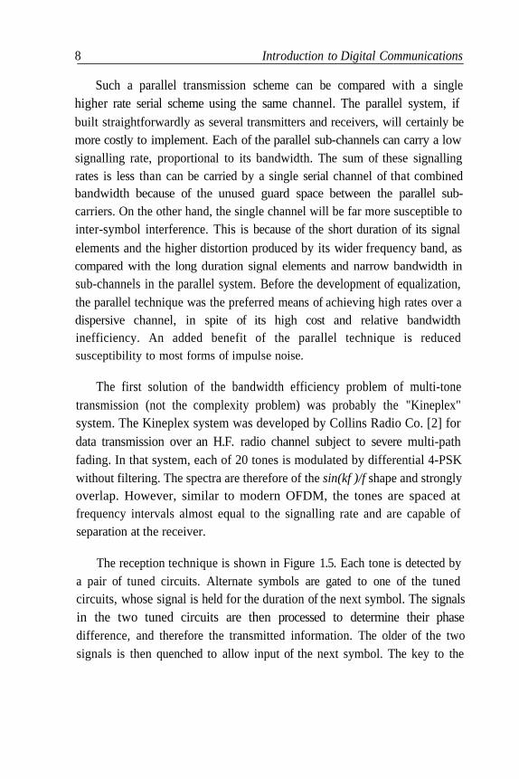
The first solution of the bandwidth efficiency problem of multi-tonetransmission (not the complexity problem) was probably the "Kineplex"system. The Kineplex system was developed by Collins Radio Co. [2] fordata transmission over an H.F. radio channel subject to severe multi-pathfading. In that system, each of 20 tones is modulated by differential 4-PSKwithout filtering. The spectra are therefore of the sin(kf )/f shape and stronglyoverlap. However, similar to modern OFDM, the tones are spaced atfrequency intervals almost equal to the signalling rate and are capable ofseparation at the receiver.
The reception technique is shown in Figure 1.5. Each tone is detected bya pair of tuned circuits. Alternate symbols are gated to one of the tunedcircuits, whose signal is held for the duration of the next symbol. The signalsin the two tuned circuits are then processed to determine their phasedifference, and therefore the transmitted information. The older of the twosignals is then quenched to allow input of the next symbol. The key to the

Introduction to Digital Communications 9
success of the technique is that the time response of each tuned circuit to alltones, other than the one to which it is tuned, goes through zero at the end ofthe gating interval, at which point that interval is equal to the reciprocal ofthe frequency separation between tones. The gating time is made somewhatshorter than the symbol period to reduce inter-symbol interference, but
efficiency of 70% of the Nyquist rate is achieved. High performance overactual long H.F. channels was obtained, although at a high implementationcost. Although fully transistorized, the system required two large bays ofequipment.
Figure 1.5. The Collins Kineplex receiver.
A subsequent multi-tone system [3] was proposed using 9-point QAMconstellations on each carrier, with correlation detection employed in thereceiver. Carrier spacing equal to the symbol rate provides optimum spectralefficiency. Simple coding in the frequency domain is another feature of thisscheme.

10 Introduction to Digital Communications
The above techniques do provide the orthogonality needed to separatemulti-tone signals spaced by the symbol rate. However the sin(kf )/f spectrumof each component has some undesirable properties. Mutual overlap of alarge number of sub-channel spectra is pronounced. Also, spectrum for theentire system must allow space above and below the extreme tonefrequencies to accommodate the slow decay of the sub-channel spectra. Forthese reasons, it is desirable for each of the signal components to bebandlimited so as to overlap only the immediately adjacent sub-carriers,while remaining orthogonal to them. Criteria for meeting this objective aregiven in References [4] and [5].
Figure 1.6. An early version of OFDM.
In Reference [6] it was shown how bandlimited QAM can be employedin a multi-tone system with orthogonality and minimum carrier spacing

Introduction to Digital Communications 11
(illustrated in Figure 1.6). Unlike the non-bandlimited OFDM, each carriermust carry Staggered (or Offset) QAM, that is, the input to the I and Qmodulators must be offset by half a symbol period. Furthermore, adjacent
carriers must be offset oppositely. It is interesting to note that StaggeredQAM is identical to Vestigial Sideband (VSB) modulation. The low-pass
filters g( t ) are such that the combination of transmit and receivefilters, is Nyquist, with the roll-off factor assumed to be less than 1.
Figure 1.7. OFDM modulation concept: Real and Imaginery components ofan OFDM symbol is the superposition of several harmonics modulated by
data symbols.
The major contribution to the OFDM complexity problem was theapplication of the Fast Fourier Transform (FFT) to the modulation anddemodulation processes [7]. Fortunately, this occurred at the same timedigital signal processing techniques were being introduced into the design of
12 Introduction to Digital Communications
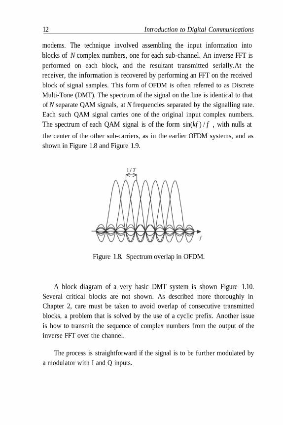
modems. The technique involved assembling the input information intoblocks of N complex numbers, one for each sub-channel. An inverse FFT isperformed on each block, and the resultant transmitted serially.At thereceiver, the information is recovered by performing an FFT on the receivedblock of signal samples. This form of OFDM is often referred to as Discrete
Multi-Tone (DMT). The spectrum of the signal on the line is identical to thatof N separate QAM signals, at N frequencies separated by the signalling rate.Each such QAM signal carries one of the original input complex numbers.
The spectrum of each QAM signal is of the form sin(kf ) / f , with nulls at
the center of the other sub-carriers, as in the earlier OFDM systems, and asshown in Figure 1.8 and Figure 1.9.
Figure 1.8. Spectrum overlap in OFDM.
A block diagram of a very basic DMT system is shown Figure 1.10.Several critical blocks are not shown. As described more thoroughly inChapter 2, care must be taken to avoid overlap of consecutive transmittedblocks, a problem that is solved by the use of a cyclic prefix. Another issueis how to transmit the sequence of complex numbers from the output of theinverse FFT over the channel.
The process is straightforward if the signal is to be further modulated bya modulator with I and Q inputs.

Introduction to Digital Communications 13
Figure 1.9. Spectrum of OFDM signal.
Otherwise, it is necessary to transmit real quantities. This can beaccomplished by first appending the complex conjugate to the original inputblock. A 2N-point inverse FFT now yields 2N real numbers to be transmittedper block, which is equivalent to N complex numbers.
Figure 1.10. Very basic OFDM system.
The most significant advantage of this DMT approach is the efficiencyof the FFT algorithm. An N-point FFT requires only on the order of N log N
multiplications, rather than as in a straightforward computation. Theefficiency is particularly good when N is a power of 2, although that is notgenerally necessary. Because of the use of the FFT, a DMT system typically
14 Introduction to Digital Communications
requires fewer computations per unit time than an equivalent single channelsystem with equalization. An overall cost comparison between the twosystems is not as clear, but the costs should be approximately equal in mostcases. It should be noted that the bandlimited system of Figure 1.6 can alsobe implemented with FFT techniques [8], although the complexity and delay
will be greater than DMT.
Over the last 20 years or so, OFDM techniques and, in particular, theDMT implementation, has been used in a wide variety of applications [9].Several OFDM voiceband modems have been introduced, but did notsucceed commercially because they were not adopted by standards bodies.DMT has been adopted as the standard for the Asymmetric DigitalSubscriber Line (ADSL), which provides digital communication at severalMb/s from a telephone company central office to a subscriber, and a lowerrate in the reverse direction, over a normal twisted pair of wires in the loopplant.
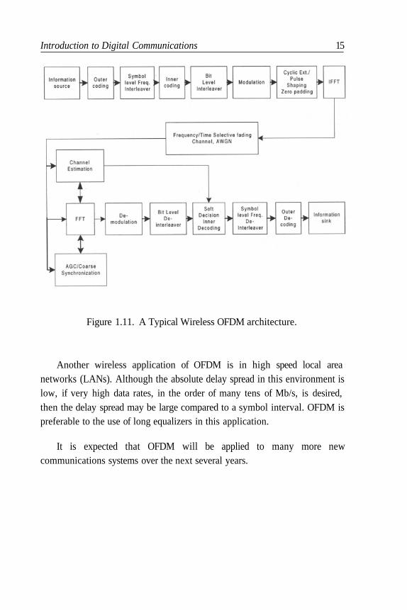
OFDM has been particularly successful in numerous wirelessapplications, where its superior performance in multi-path environments isdesirable. Wireless receivers detect signals distorted by time and frequencyselective fading. OFDM in conjunction with proper coding and interleavingis a powerful technique for combating the wireless channel impairments thata typical OFDM wireless system might face, as is shown in Figure 1.11.
A particularly interesting configuration, discussed in Chapter 10, is theSingle Frequency Network (SFN) used for broadcasting of digital audio orvideo signals. Here many geographically separated transmitters broadcastidentical and synchronized signals to cover a large region. The reception ofsuch signals by a receiver is equivalent to an extreme form of multi-path.OFDM is the technology that makes this configuration viable.
Introduction to Digital Communications 15
Figure 1.11. A Typical Wireless OFDM architecture.
Another wireless application of OFDM is in high speed local areanetworks (LANs). Although the absolute delay spread in this environment islow, if very high data rates, in the order of many tens of Mb/s, is desired,then the delay spread may be large compared to a symbol interval. OFDM ispreferable to the use of long equalizers in this application.
It is expected that OFDM will be applied to many more newcommunications systems over the next several years.
16 Introduction to Digital Communications
References
1. Gitlin, R.D., Hayes J.F., Weinstein S.B. Data Communications Principles. New York:Plenum, 1992.
2. Doelz, M.L., Heald E.T., Martin D.L. "Binary Data Transmission Techniques for LinearSystems." Proc. I.R.E.; May 1957; 45: 656-661.
3. Franco, G.A., Lachs G. "An Orthogonal Coding Technique for Communications." I. R.E. Int. Conv. Rec.; 1961; 8: 126-133.
4. Chang, R.W. "Synthesis of Band-Limited Orthogonal Signals for Multichannel DataTransmission." Bell Sys. Tech. J.; Dec 1966; 45: 1775-1796.
5. Shnidman, D.A. "A Generalized Nyquist Criterion and an Optimum Linear Receiver fora Pulse Modulation System." Bell Sys. Tech. J.; Nov 1966; 45: 2163-2177.
6. Saltzberg, B.R. "Performance of an Efficient Parallel Data Transmission System." IEEETrans. Commun.; Dec 1967; COM-15; 6: 805-811.
7. Weinstein, S.B., Ebert P.M. "Data Transmission By Frequency Division MultiplexingUsing the Discrete Fourier Transform." IEEE Trans. Commun., Oct 1971; COM-19; 5:628-634.
8. Hirosaki, B. "An Orthogonally Multiplexed QAM System Using the Discrete FourierTransform." IEEE Trans. Commun.; Jul 1981; COM-29; 7: 982-989.
9. Bingham, J.A.C. "Multicarrier Modulation for Data Transmission: An Idea Whose TimeHas Come." IEEE Commun. Mag., May 1990; 28: 5-14.

Chapter 2 System Architecture
This chapter presents a general overview of system design for multi-
carrier modulation. First, a review of the OFDM system is discussed, thenmajor system blocks will be analyzed.
2.1 Multi-Carrier System Fundamentals
Let denote data symbols. Digital signal processing
techniques, rather than frequency synthesizers, can be deployed to generateorthogonal sub-carriers. The DFT as a linear transformation maps the
complex data symbols to OFDM symbols
such that
The linear mapping can be represented in matrix form as:
17
18 System Architecture
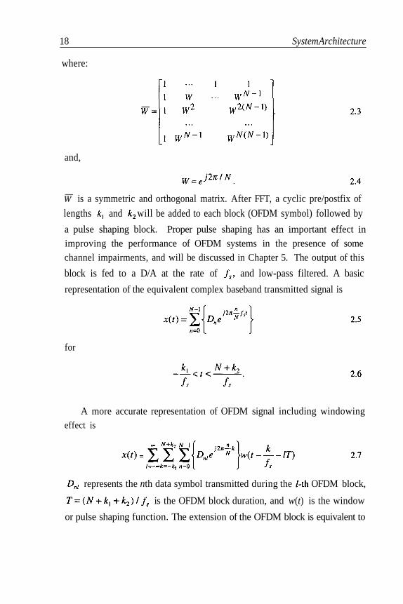
where:
and,
is a symmetric and orthogonal matrix. After FFT, a cyclic pre/postfix of
lengths and will be added to each block (OFDM symbol) followed by
a pulse shaping block. Proper pulse shaping has an important effect inimproving the performance of OFDM systems in the presence of somechannel impairments, and will be discussed in Chapter 5. The output of this
block is fed to a D/A at the rate of and low-pass filtered. A basic
representation of the equivalent complex baseband transmitted signal is
for
A more accurate representation of OFDM signal including windowingeffect is
represents the nth data symbol transmitted during the OFDM block,
is the OFDM block duration, and w(t) is the window
or pulse shaping function. The extension of the OFDM block is equivalent to
System Architecture 19
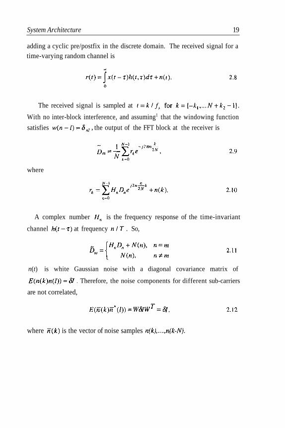
adding a cyclic pre/postfix in the discrete domain. The received signal for atime-varying random channel is
The received signal is sampled at
With no inter-block interference, and assuming1 that the windowing function
satisfies the output of the FFT block at the receiver is
where
A complex number is the frequency response of the time-invariant
channel at frequency . So,
n(t) is white Gaussian noise with a diagonal covariance matrix of
Therefore, the noise components for different sub-carriers
are not correlated,
where is the vector of noise samples
20 System Architecture
A detailed mathematical analysis of OFDM in multi-path Rayleighfading is presented in the Appendix.
2.2 DFT
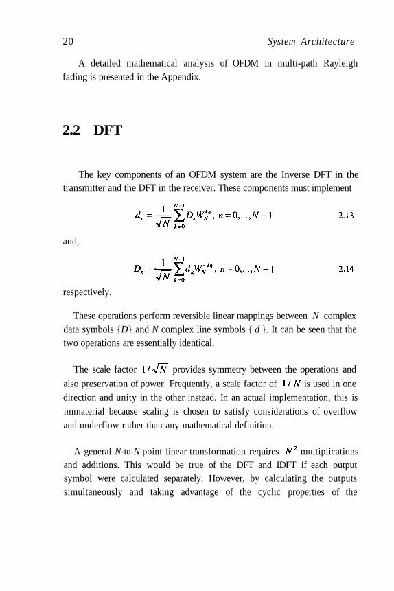
The key components of an OFDM system are the Inverse DFT in thetransmitter and the DFT in the receiver. These components must implement
and,
respectively.
These operations perform reversible linear mappings between N complexdata symbols {D} and N complex line symbols { d }. It can be seen that thetwo operations are essentially identical.
The scale factor provides symmetry between the operations andalso preservation of power. Frequently, a scale factor of is used in onedirection and unity in the other instead. In an actual implementation, this isimmaterial because scaling is chosen to satisfy considerations of overflowand underflow rather than any mathematical definition.
A general N-to-N point linear transformation requires multiplicationsand additions. This would be true of the DFT and IDFT if each outputsymbol were calculated separately. However, by calculating the outputssimultaneously and taking advantage of the cyclic properties of the

System Architecture 21
multipliers Fast Fourier Transform (FFT) techniques reduce the
number of computations to the order of N log N . The FFT is most efficient
when N is a power of two. Several variations of the FFT exist, with differentordering of the inputs and outputs, and different use of temporary memory.One variation, decimation in time, is shown below.
Figure 2.1. An FFT implementation (decimation in time).
Figure 2.2 shows the architecture of an OFDM system capable of using afurther stage of modulation employing both in-phase and quadraturemodulators. This configuration is common in wireless communication
systems for modulating baseband signals to the required IF or RF frequency
band. It should be noted that the basic configuration illustrated does notaccount for channel dispersion, which is almost always present. The channeldispersion problem is solved by using the cyclic prefix which will bedescribed later.

22 System Architecture
Figure 2.2. System with complex transmission.
Small sets of input bits are first assembled and mapped into complexnumbers which determine the constellation points of each sub-carrier. Inmost wireless systems, smaller constellation is formed for each sub-carrier.In wireline systems, where the signal-to-noise ratio is higher and variableacross the frequency range, the number of bits assigned to each sub-carriermay be variable. Optimization of this bit assignment is the subject of bitallocation, to be discussed in the next chapter.

System Architecture 23
If the number of sub-carriers is not a power of two, then it is common toadd symbols of value zero to the input block so that the advantage of usingsuch a block length in the FFT is achieved. The quantity N which determinesthe output symbol rate is then that of the padded input block rather than thenumber of sub-carriers.
The analog filters at the transmitter output and the receiver input shouldbandlimit the respective signals to a bandwidth of 1/T. Low pass filters couldbe used instead of the band-pass filters shown, placed on the other side of themodulator or demodulator. The transmit filter eliminates out-of-band powerwhich may interfere with other signals. The receive filter is essential to avoidaliasing effects. The transmitted signal has a continuous spectrum whosesamples at frequencies spaced 1/T apart agree with the mapped input data. Inparticular, the spectrum of each sub-carrier is the form sinc(1/T), whosecentral value is that input value, and whose nulls occur at the centralfrequencies of all other sub-carriers.
The receiver operations are essentially the reverse of those in thetransmitter. A critical set of functions, however, are synchronization ofcarrier frequency, sampling rate, and block framing. There is a minimumdelay of 2T through the system because of the block assembly functions inthe transmitter and receiver.
The FFT functions may be performed either by a general purpose DSPor special circuitry, depending primarily on the information rate to becarried. Some simplification compared with full multiplication may bepossible at the transmitter, by taking advantage of small constellation sizes.
The number of operations per block of duration T is where
K is a small quantity. To compare this with a single carrier system, the
number of operations per line symbol interval T/N is which is
substantially below the requirement of an equalizer in a typical single carrierimplementation for wireline applications.
24 System Architecture
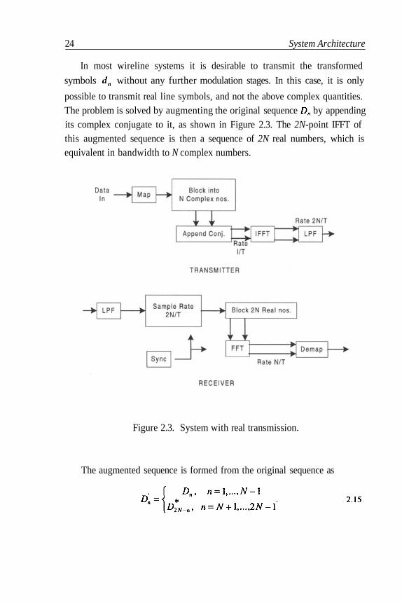
In most wireline systems it is desirable to transmit the transformed
symbols without any further modulation stages. In this case, it is only
possible to transmit real line symbols, and not the above complex quantities.The problem is solved by augmenting the original sequence by appendingits complex conjugate to it, as shown in Figure 2.3. The 2N-point IFFT ofthis augmented sequence is then a sequence of 2N real numbers, which isequivalent in bandwidth to N complex numbers.
Figure 2.3. System with real transmission.
The augmented sequence is formed from the original sequence as
System Architecture 25
In order to maintain conjugate symmetry, it is essential that and
be real. If the original is zero, as is common, then and are set to
zero. Otherwise, may be set to and to
For the simple case of the output of the IFFT is:
where Of course the scaling by a factor of two is immaterialand can be dropped. This real orthogonal transformation is fully equivalentto the complex one, and all subsequent analyses are applicable.
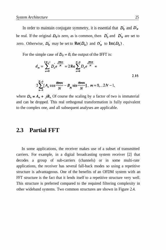
2.3 Partial FFT
In some applications, the receiver makes use of a subset of transmittedcarriers. For example, in a digital broadcasting system receiver [2] thatdecodes a group of sub-carriers (channels) or in some multi-rateapplications, the receiver has several fall-back modes so using a repetitivestructure is advantageous. One of the benefits of an OFDM system with anFFT structure is the fact that it lends itself to a repetitive structure very well.This structure is preferred compared to the required filtering complexity inother wideband systems. Two common structures are shown in Figure 2.4.

26 System Architecture
Figure 2.4. Two different techniques for FFT butterfly.
An example of partial FFT is shown in Figure 2.5. In order to detect(receive) the marked point at the output, we can restrict the FFT calculationto the marked lines. Therefore, a significant amount of processing will besaved.
Figure 2.5. Partial FFT (DIT)
Two main differences between decimation in time (DIT) and decimationin frequency (DIF) are noted [1]. First, for DIT, the input is bit-reversed andoutput is in natural order, while in DIF the reverse is true. Secondly, for DIT
System Architecture 27
complex multiplication is performed before the add-subtract operation, whilein DIF the order is reversed. While complexity of the two structures issimilar in typical DFT, this is not the case for partial FFT [2]. The reason isthat in the DIT version of partial FFT, a sign change (multiplication by 1 and-1) occurs at the first stages, but in the DIF version it occurs in later stages.
2.4 Cyclic Extension
Transmission of data in the frequency domain using an FFT, as acomputationally efficient orthogonal linear transformation, results inrobustness against ISI in the time domain. Unlike the Fourier Transform(FT), the DFT (or FFT) of the circular convolution of two signals is equal to
the product of their DFT's (FFT).
where and denote linear and circular convolution respectively.
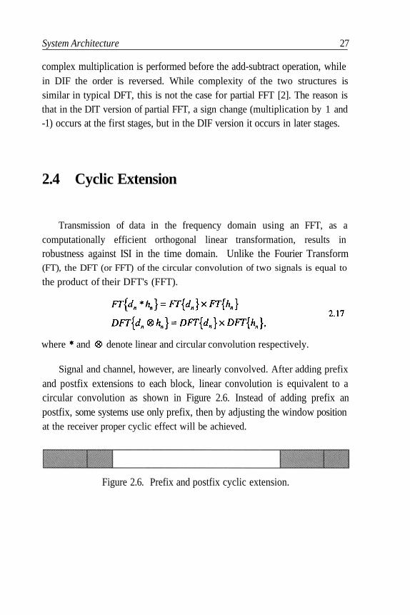
Signal and channel, however, are linearly convolved. After adding prefix
and postfix extensions to each block, linear convolution is equivalent to acircular convolution as shown in Figure 2.6. Instead of adding prefix anpostfix, some systems use only prefix, then by adjusting the window positionat the receiver proper cyclic effect will be achieved.
Figure 2.6. Prefix and postfix cyclic extension.

28 System Architecture
Using this technique, a signal, otherwise aliased, appears infinitelyperiodic to the channel. Let’s assume the channel response is spread over Msamples, and the data block has N samples then:
where is a rectangular window of length N . To describe the effect
of distortion, we proceed with the Fourier Transform noting that convolutionis linear
After linear convolution of the signal and channel impulse response, thereceived sequence is of length The sequence is truncated to N
samples and transformed to the frequency domain, which is equivalent toconvolution and truncation. However, in the case of cyclic pre/postfixextension, the linear convolution is the same as the circular convolution aslong as channel spread is shorter than guard interval. After truncation, theDFT can be applied, resulting in a sequence of length N because thecircular convolution of the two sequences has period of N .
Intuitively, an N -point DFT of a sequence corresponds to a Fourierseries of the periodic extension of the sequence with a period of N. So, inthe case of no cyclic extension we have
which is equivalent to repeating a block of length with periodN .This results in aliasing or inter-symbol interference between adjacentOFDM symbols. In other words, the samples close to the boundaries of each

System Architecture 29
symbol experience considerable distortion, and with longer delay spread,more samples will be affected. Using cyclic extension, the convolutionchanges to a circular operation. Circular convolution of two signals of lengthN is a sequence of length N so the inter-block interference issue isresolved.
Proper windowing of OFDM blocks, as shown later, is important tomitigate the effect of frequency offset and to control transmitted signalspectrum. However, windowing should be implemented after cyclicextension of the frame, so that the windowed frame is not cyclicallyextended. A solution to this problem is to extend each frame to 2N points atthe receiver and implement a 2N FFT. Practically, it requires a 2N IFFTblock at the transmitter, and 2N FFT at the receiver. However, by usingpartial FFT techniques, we can reduce the computation by calculating onlythe required frequency bins.
If windowing was not required, we could have simply used zero paddedpre/postfix, and before the DFT at the receiver copy the beginning and endof frame as prefix and postfix. This creates the same effect of cyclicextension with the advantage of reducing transmit power and causing lessISI.
The relative length of cyclic extension depends on the ratio of thechannel delay spread to the OFDM symbol duration.
2.5 Channel Estimation
Channel estimation inverts the effect of non-selective fading on each sub-carrier. Usually, OFDM systems provide pilot signals for channel estimation.In the case of time-varying channels the pilot signal should be repeatedfrequently. The spacing between pilot signals in time and frequency depends
30 System Architecture
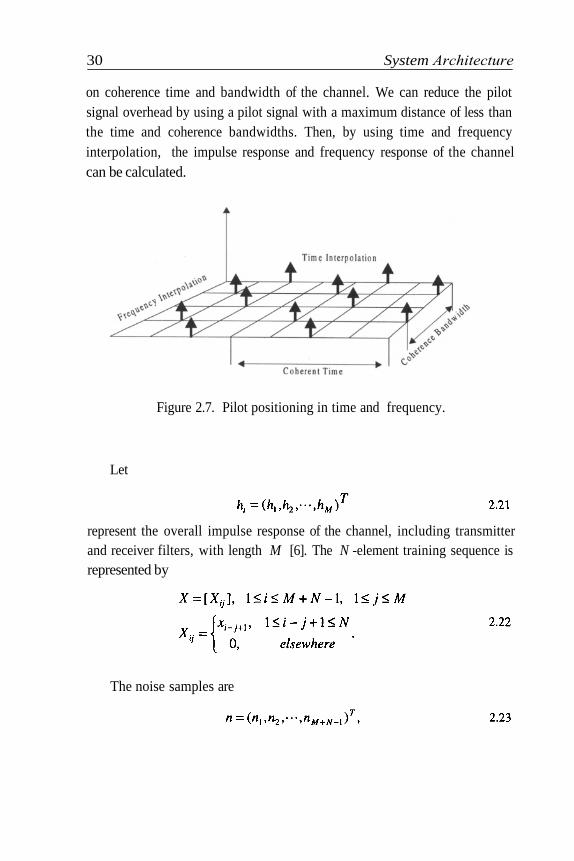
on coherence time and bandwidth of the channel. We can reduce the pilotsignal overhead by using a pilot signal with a maximum distance of less thanthe time and coherence bandwidths. Then, by using time and frequencyinterpolation, the impulse response and frequency response of the channelcan be calculated.
Figure 2.7. Pilot positioning in time and frequency.
Let
represent the overall impulse response of the channel, including transmitterand receiver filters, with length M [6]. The N -element training sequence isrepresented by
The noise samples are

System Architecture 31
with
in which L is a lower triangular matrix, which can be calculated by theCholesky method. The received signal is then
After correlation or matched filtering, the estimate of the impulseresponse is:
If the additive noise is white, the matched filter is the best estimator interms of maximizing signal-to-noise ratio. However, the receiver filter colorsthe noise. With a whitening filter the estimate is given in [5]. An unbiasedestimator, which removes the effect of sidelobes, is [5]
In the dual system architecture, circular convolution is replaced bymultiplication. The repetition of the training sequence results in circularconvolution. Therefore, Equation 2.26 is replaced by:
where superscript shows Fourier Transform and all products are scalar.The same procedure can be applied to Equation 2.27. This procedure is alsocalled frequency equalization.
32 System Architecture
2.6 Appendix — Mathematical Modelling ofOFDM for Time-Varying Random Channel
Characterization of Randomly Time-VaryingChannels
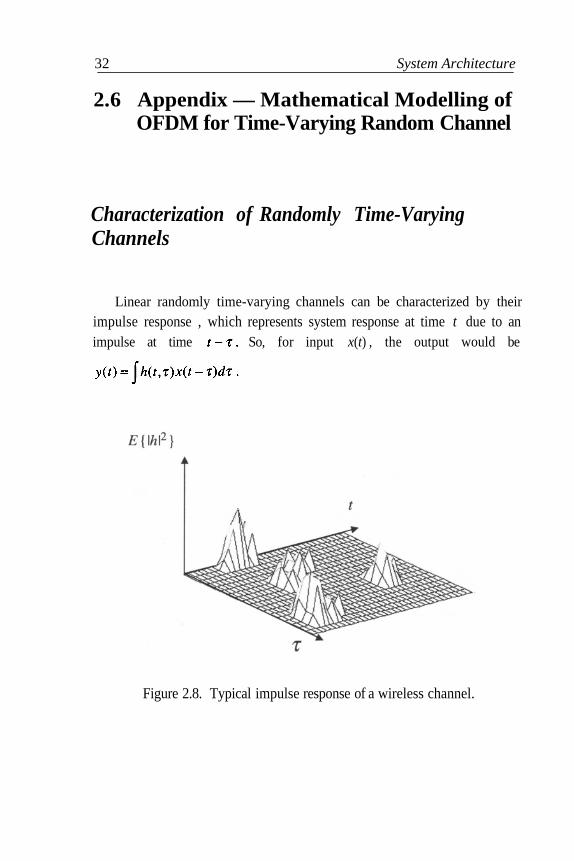
Linear randomly time-varying channels can be characterized by theirimpulse response , which represents system response at time t due to animpulse at time So, for input x(t) , the output would be
Figure 2.8. Typical impulse response of a wireless channel.
System Architecture 33
Other kernels can be defined to relate input and output in time andfrequency domains [3]. Since the impulse response is time-varying, it isexpected that the system transfer function is time-varying. The transferfunction is defined as
If the input is a single tone the output is:
which shows that the time-varying transfer function has an interpretationsimilar to time-invariant systems. Namely, the output of the system for asinusoidal function is the input multiplied by the transfer function. Ingeneral, is a random process and its exact statistical description
requires a multi-dimensional probability distribution. A practicalcharacterization of the channel is given by first and second order momentsof system functions. For example, many randomly time-varying physicalchannels are modelled as wide sense stationary non-correlated scatterers.Therefore, they are white and non-stationary with respect to delay variableand stationary with respect to t.
is called the tap gain correlation. The scattering function of the
channel is defined as
For any fixed the scattering function may be regarded as the complex-valued spectrum of the system. The relationship between different systemfunctions is shown in the Figure 2.9 and Figure 2.10.

34 System Architecture
Figure 2.9. Relationship between system functions.
Figure 2.10. Relationship between correlation functions.
Coherence bandwidth of the received signal (or channel) is defined as thefrequency distance beyond which frequency responses of the signal areuncorrelated. The reciprocal of delay spread is an estimate for coherencebandwidth. Coherence time is the time distance beyond which the samples ofreceived signal (or channel impulse response) are uncorrelated. Since thechannel and signal are Gaussian, independence of samples is equivalent totheir being non-correlated. The reciprocal of Doppler spread is an estimateof coherence time [4].
OFDM in Randomly Time-Varying Channels
In general, OFDM is a parallel transmission technique in which N
complex symbols modulate N orthogonal waveforms which maintain
their orthogonality at the output of the channel. This requires that thecorrelation function of the channel output process, in response to different
waveforms, has orthogonal eigenfunctions.
System Architecture 35
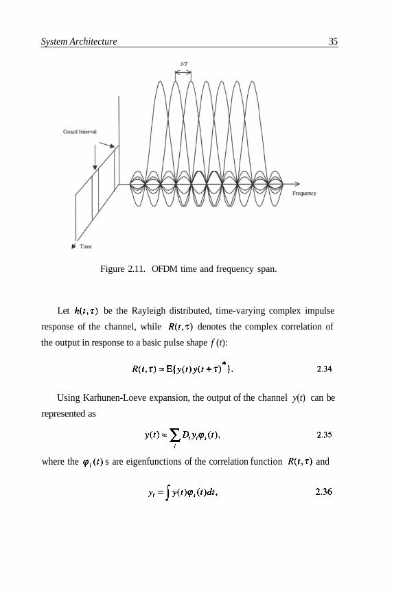
Figure 2.11. OFDM time and frequency span.
Let be the Rayleigh distributed, time-varying complex impulse
response of the channel, while denotes the complex correlation of
the output in response to a basic pulse shape f (t):
Using Karhunen-Loeve expansion, the output of the channel y(t) can be
represented as
where the s are eigenfunctions of the correlation function and

36 System Architecture
Figure 2.12. Time-varying channel.
Using Karhunen-Loeve expansion, the output of the channel y(t) can be
represented as
where the are eigenfunctions of the correlation function and
The corresponding eigenvalues of the correlation function are where
For a Gaussian random process y(t), the coefficients in Equation 2.37
are Gaussian random variables and their powers are the correspondingeigenvalues. If the input consists of orthogonal modulating functions whichare harmonics of the form
where u(t) is the basic waveform such as time-limted gating function. The
eigenfunctions of the received signal correlation function are,
where again are the eigenfunctions’ output correlation functions in
response to basic waveform u(t). Therefore, the orthogonality condition is
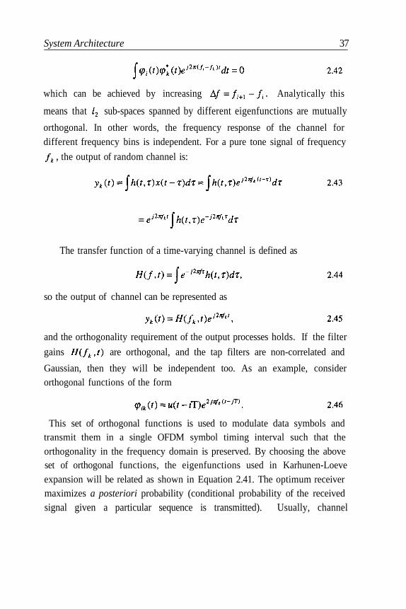
System Architecture 37
which can be achieved by increasing Analytically this
means that sub-spaces spanned by different eigenfunctions are mutually
orthogonal. In other words, the frequency response of the channel fordifferent frequency bins is independent. For a pure tone signal of frequency
the output of random channel is:
The transfer function of a time-varying channel is defined as
so the output of channel can be represented as
and the orthogonality requirement of the output processes holds. If the filter
gains are orthogonal, and the tap filters are non-correlated and
Gaussian, then they will be independent too. As an example, considerorthogonal functions of the form
This set of orthogonal functions is used to modulate data symbols andtransmit them in a single OFDM symbol timing interval such that the
orthogonality in the frequency domain is preserved. By choosing the aboveset of orthogonal functions, the eigenfunctions used in Karhunen-Loeveexpansion will be related as shown in Equation 2.41. The optimum receivermaximizes a posteriori probability (conditional probability of the receivedsignal given a particular sequence is transmitted). Usually, channel

38 System Architecture
characteristics do not change during one or a few symbols. Therefore, thechannel output can be represented as
The received signal with n(t) representing additive
white Gaussian noise can be expanded as
where
Notice that the noise projection should be interpreted as a stochastic
integral, because a Riemann integral is not defined for white noise. are
independent zero mean Gaussian random variables and their powers are
assuming that data symbols are of equal and unit power. So, the problem athand reduces to the detection of a Gaussian random process corrupted byGaussian noise.
References
1. Rabiner, L.R., Gold B. Theory and Application of Digital Signal Processing. EnglewoodCliffs, NJ: Prentice Hall, 1975.

System Architecture 39
2. Alard, M., Lassalle R. "Principles of Modulation and Channel Coding for DigitalBroadcasting for Mobile Receivers." EBU Review; Aug 1987; 224: 47-68
3. Bello, P.A. "Characterization of Randomly Time-Variant Linear Channels", IEEE TransComm; Dec 1963; COM-11; 360-393.
4. Kennedy, R.S. Fading Dispersive Communication Channels. New York: WileyInterscience, 1969.
5. Bahai, A.R.S. "Estimation in Randomly Time-Varying Systems with Applications toDigital Communications." Ph.D. Dissertation, Univ. of California at Berkeley, 1993.
6. Klein, A., Mohr, W. "Measurement-Based Parameter Adaptation of Wideband SpatialMobile Radio Channel Models." IEEE 4th International Symp. on Spread SpectrumTechniques and App. Proc., ISSSTA'95, 91-97

Chapter 3 Performance Over Time-Invariant Channels
3.1 Time-Invariant Non-Flat Channel withColored Noise
Many channels, such as wireline, have transmission properties and noisestatistics that vary very slowly with time. Therefore, over moderately longtime intervals they may be treated as being invariant. In such a case, thechannel impulse response is a function only of and may be
written as h(u) where Since it is a function of only one variable,
we may take its 1-dimensional Fourier Transform to arrive at the channel
transfer function
41
Similarly the auto-correlation of the noise is also a function only
of and can be treated as Its Fourier Transform N(f) is the
power spectral density. Since, in general, both and N(f) vary over thefrequency band of interest, the signal-to-noise ratio also varies.
We are now ready to analyze the performance of a multi-carrier systemover such a channel, and to optimize the transmitted signal so as tomaximize performance.
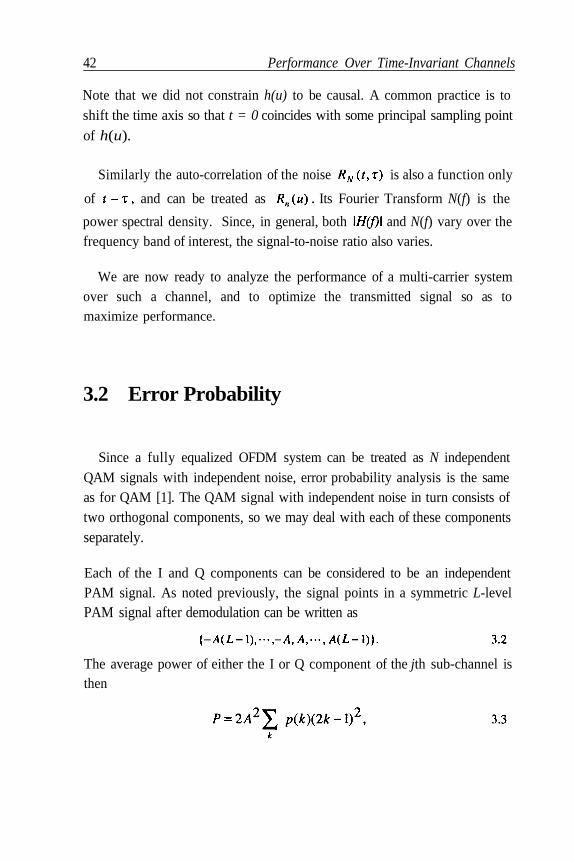
3.2 Error Probability
Since a fully equalized OFDM system can be treated as N independentQAM signals with independent noise, error probability analysis is the sameas for QAM [1]. The QAM signal with independent noise in turn consists oftwo orthogonal components, so we may deal with each of these componentsseparately.
Each of the I and Q components can be considered to be an independentPAM signal. As noted previously, the signal points in a symmetric L-levelPAM signal after demodulation can be written as
The average power of either the I or Q component of the jth sub-channel isthen
42 Performance Over Time-Invariant Channels
Note that we did not constrain h(u) to be causal. A common practice is toshift the time axis so that t = 0 coincides with some principal sampling point
of h(u).
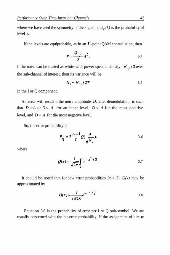
If the levels are equiprobable, as in an -point QAM constellation, then
If the noise can be treated as white with power spectral density over
the sub-channel of interest, then its variance will be
where
It should be noted that for low error probabilities (x > 3), Q(x) may beapproximated by
Equation 3.6 is the probability of error per I or Q sub-symbol. We areusually concerned with the bit error probability. If the assignment of bits to
Performance Over Time-Invariant Channels 43
where we have used the symmetry of the signal, and p(k) is the probability oflevel k.
in the I or Q component.
An error will result if the noise amplitude D, after demodulation, is such
that D >A or D<–A for an inner level, D<–A for the most positive
level, and D > A for the most negative level.
So, the error probability is
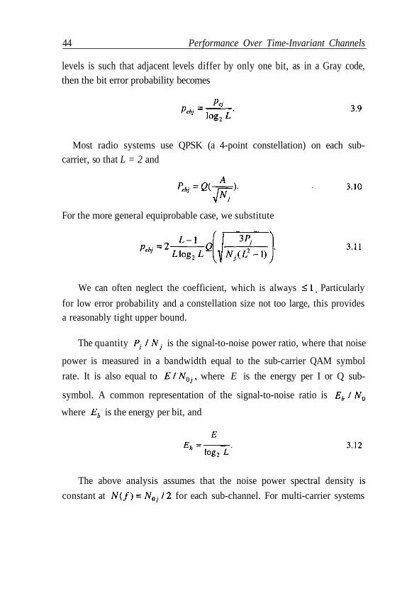
Most radio systems use QPSK (a 4-point constellation) on each sub-carrier, so that L = 2 and
For the more general equiprobable case, we substitute
We can often neglect the coefficient, which is always Particularly
for low error probability and a constellation size not too large, this providesa reasonably tight upper bound.
The quantity is the signal-to-noise power ratio, where that noise
power is measured in a bandwidth equal to the sub-carrier QAM symbol
rate. It is also equal to where E is the energy per I or Q sub-
symbol. A common representation of the signal-to-noise ratio is
where is the energy per bit, and
The above analysis assumes that the noise power spectral density is
constant at for each sub-channel. For multi-carrier systems
44 Performance Over Time-Invariant Channels
levels is such that adjacent levels differ by only one bit, as in a Gray code,then the bit error probability becomes
where is the receiver response for the jth sub-channel.
For straight DMT without windowing,
where is the center frequency of the sub-channel.
It is common in analyzing multi-carrier systems to deal with QAM sub-carriers rather than the I and Q components. Equation 3.11 can be written as
is the noise power in the that sub-channel after receiver processing, and Kis the average number of its nearest neighbors, and is usually (but notnecessarily) an integer.
Equation 3.15 is strictly applicable to square equiprobable constellations.However, very little error will result if we instead use the same analysis formore general equiprobable constellations. For example, a large QAMconstellation with a circular boundary will have only 0.2 dB less averagepower than a square constellation with the same number of points andspacing between points. If further "shaping gain" is provided by using amulti-dimensional hyperspheric constellation boundary over several QAMsub-channels, then up to 1.53 dB average power reduction can be achieved.However, such shaping gain is rarely used in OFDM systems.
Performance Over Time-Invariant Channels 45
with a large number of sub-channels, this should be an excellentapproximation. When this is not the case, we should use
where is the number of points in the QAM constellation, is its power,
For a complete OFDM system, the overall average bit error probability is
Clearly if the are all equal, that will also be the overall errorprobability. Otherwise, the higher error probabilities will dominateperformance. A sensible design goal is, therefore, to try to achieve the sameerror probabilities on all sub-channels if possible.
3.3 Bit Allocation
We now address the problem of optimizing the performance of anOFDM system over a stationary, non-flat, linear channel through choice ofthe transmitted signal. We may either seek to maximize the overall bit ratewith a required error probability, or we may minimize the error probabilityfor a given bit rate. We will first deal with the former optimization, that is,
the maximization of
where is the number of bits carried by the constellation of the j th sub-
carrier. We will deal primarily with the case of high signal-to-noise ratio(low error probability).
46 Performance Over Time-Invariant Channels
channels, separated in frequency by is assumed to be small
enough so that the channel gain and the noise power spectral
density are constant over each of the sub-channels. So, the channel gain and
noise power on the jth sub-channel can be given by and
respectively. It is assumed that the noise is Gaussian. This assumption mayseem questionable when the noise is primarily due to crosstalk, as on mostcabled wire-pair media. However the assumption becomes valid when thereare many such interferers, and/or when they are passed through a narrowfilter, as is the case in OFDM.
. The variables in the optimization are the individually transmitted sub-
It would appear that the constraint of an overall error probability is bestmet by requiring that same error probability for each of the sub-channels.This is indeed true at low error probabilities, which is the condition understudy here, but it has recently been shown [2] that this is, in general, sub-optimum. A further simplification that is usually made is to constrain thesymbol error probability of each sub-channel to the target value, rather thanthe bit error probability. This can be significantly pessimistic, but thedifference in required signal-to-noise ratio is not too great at very low errorprobabilities, or when trellis coding is used. When fine precision is desired,the difference between symbol and bit error probability can be accountedfor.
Performance Over Time-Invariant Channels 47
The total transmitted power is assumed to be constrained. We assume thatthe multi-carrier signal consists of a large number of non-interfering sub-
channel powers and the individual constellation sizes Fortunately
these optimizations are separable. We may first optimize the powerdistribution, under the constraint
This requires that we set the quantity
to the constant value such that
The problem of optimizing the transmit powers of the sub-carriers issimilar to a classical problem in information theory: given a linear channel
with transfer function H(f), Gaussian noise of power spectral density N( f ),and a transmit power constraint P, find the transmit power distribution thatmaximizes the capacity of the channel. The answer is the well-known "waterpouring" solution [3]:
where
and is the value for which
48 Performance Over Time-Invariant Channels
Setting the symbol error probability to the target value p requires that
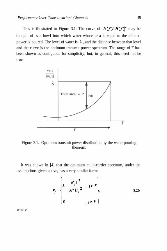
This is illustrated in Figure 3.1. The curve of may be
thought of as a bowl into which water whose area is equal to the allottedpower is poured. The level of water is , and the distance between that leveland the curve is the optimum transmit power spectrum. The range of F hasbeen shown as contiguous for simplicity, but, in general, this need not be
true.
Figure 3.1. Optimum transmit power distribution by the water pouringtheorem.
It was shown in [4] that the optimum multi-carrier spectrum, under theassumptions given above, has a very similar form:
where
Performance Over Time-Invariant Channels 49
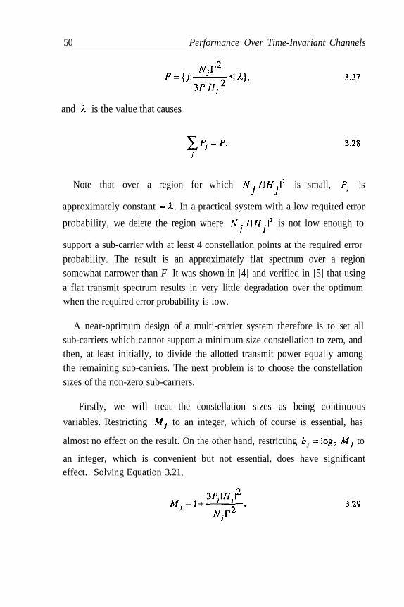
and is the value that causes
Note that over a region for which is small, is
approximately constant . In a practical system with a low required error
probability, we delete the region where is not low enough to
support a sub-carrier with at least 4 constellation points at the required error
probability. The result is an approximately flat spectrum over a regionsomewhat narrower than F. It was shown in [4] and verified in [5] that usinga flat transmit spectrum results in very little degradation over the optimumwhen the required error probability is low.
A near-optimum design of a multi-carrier system therefore is to set allsub-carriers which cannot support a minimum size constellation to zero, andthen, at least initially, to divide the allotted transmit power equally amongthe remaining sub-carriers. The next problem is to choose the constellationsizes of the non-zero sub-carriers.
Firstly, we will treat the constellation sizes as being continuousvariables. Restricting to an integer, which of course is essential, has
almost no effect on the result. On the other hand, restricting to
an integer, which is convenient but not essential, does have significanteffect. Solving Equation 3.21,
50 Performance Over Time-Invariant Channels
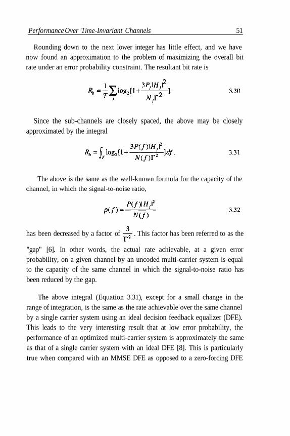
Since the sub-channels are closely spaced, the above may be closelyapproximated by the integral
The above is the same as the well-known formula for the capacity of thechannel, in which the signal-to-noise ratio,
has been decreased by a factor of This factor has been referred to as the
"gap" [6]. In other words, the actual rate achievable, at a given errorprobability, on a given channel by an uncoded multi-carrier system is equalto the capacity of the same channel in which the signal-to-noise ratio hasbeen reduced by the gap.
The above integral (Equation 3.31), except for a small change in therange of integration, is the same as the rate achievable over the same channelby a single carrier system using an ideal decision feedback equalizer (DFE).This leads to the very interesting result that at low error probability, theperformance of an optimized multi-carrier system is approximately the sameas that of a single carrier system with an ideal DFE [8]. This is particularlytrue when compared with an MMSE DFE as opposed to a zero-forcing DFE
Performance Over Time-Invariant Channels 51
Rounding down to the next lower integer has little effect, and we havenow found an approximation to the problem of maximizing the overall bitrate under an error probability constraint. The resultant bit rate is

Now define an average signal-to noise ratio [6] such that
Then, with n the number of sub-channels,
and at high signal-to-noise ratio,
Thus, at high signal-to-noise ratio, when a multi-carrier system is fullyoptimized, the average signal-to-noise ratio is the geometric mean of thesignal-to-noise ratios of the sub-channels. This is an important quantity, andserves as a good quality measure of the channel. The integral form of theabove appears in analyses of single carrier systems with DFE.
So far we have not required that the number of bits carried by each sub-carrier be an integer. Such non-integral values can be achieved by treatingmore than one sub-carrier as a constellation in a higher-dimensional space,and assigning an integral number of bits to that higher-dimensionalconstellation. However, to avoid that complexity, it is usually required thatbe an integer. Simply performing the above optimization and rounding each
down results in the average loss of bit per sub-carrier.
52 Performance Over Time-Invariant Channels
[9]. At higher error probabilities, the multi-carrier system has been shown toperform somewhat better [2].
We can rewrite Equation 3.30 as:
maximizing a variable bit rate. As before, we first determine such that
where p is the desired error probability, and is conservatively
Performance Over Time-Invariant Channels 53
The above loss can be mostly recovered by small adjustments in the sub-carrier powers. Those sub-carriers that required a large round-down can havetheir powers increased slightly in order to achieve one more bit. Those witha smaller round-down can have their power reduced while keeping the samenumber of bits. During this process of power re-allocation, it is important toensure that the constraint of total power is kept. After the process iscompleted, the power deviations will vary over a 3 dB range.
A further small increase in bit rate can be achieved by accounting for thebit error probability of each sub-carrier rather than the symbol errorprobability, which is higher. This involves calculating the bit errorprobability for each sub-carrier after the system has been optimized forsymbol error probability. Those sub-carriers which can meet the bit errorprobability target with an addition bit can then have their constellationsincreased accordingly.
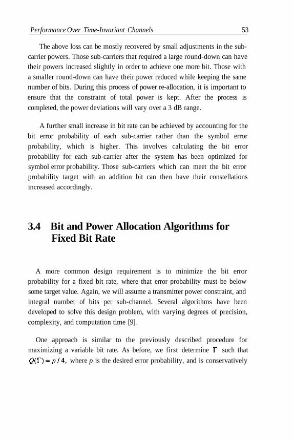
3.4 Bit and Power Allocation Algorithms forFixed Bit Rate
A more common design requirement is to minimize the bit errorprobability for a fixed bit rate, where that error probability must be belowsome target value. Again, we will assume a transmitter power constraint, andintegral number of bits per sub-channel. Several algorithms have beendeveloped to solve this design problem, with varying degrees of precision,complexity, and computation time [9].
One approach is similar to the previously described procedure for
is greater than the required rate. If not, the desired performance cannot be
achieved. Otherwise, if where B is the required bit rate, A is a
positive integer, and J is the number of used sub-carriers, then A bits aresubtracted from each sub-carrier. This step adds 3 dB of noise margin.
After the above procedure, the number of bits on each sub-carrier is
rounded down to the next lowest integer. The resultant bit rate R' is
compared with B. If then a set of sub-carriers with the smallest
round-off are each reduced by an additional bit. If then a set of sub-carriers with the largest round-off are each increased by one bit. Finally, thepowers of the sub-carriers are adjusted as before to achieve the same errorprobability for each.
References
1. Gitlin, R.D., Hayes J.F., Weinstein S.B. Data Communications Principles. New York:Plenum, 1992.
2. Willink, T.J., Wittke P.M. "Optimization and Performance Evaluation of Multi-CarrierTransmission." IEEE Irons. Info. Theory; Mar 1997; 43: 426-440.
3. Gallagher, R.G. Information Theory and Reliable Communication. New York: Wiley,1968.
4. Kalet, I. "The Multitone Channel." IEEE Trans. Commun.; Feb 1989; 37: 119-124.
5. Feig, E. "Practical Aspects of DFT-Based Frequency Division Multiplexing for DataTransmission." IEEE Trans. Commun.; Jul 1990; 38: 929-932.
54 Performance Over Time-Invariant Channels
chosen as the maximum symbol error probability for each sub-carrier. Wenow examine if the unquantized total bit rate

Performance Over Time-Invariant Channels 55
6. Sistanizadeh, K., Chow P.S., Cioffi J.M. "Multi-Tone Transmission for ADSL." IEEEInt. Conf. Commun.; 1993; 756-760.
7. Chow, P.S., Cioffi J.M., Bingham J.A.C. "A Practical Discrete Multitone TransceiverLoading Algorithm for Data Transmission Over Spectrally Shaped Channels." IEEETrans. Commun., Feb-Apr 1995; 43: 773-775.
8. Zervos, N.A., Kalet I. "Optimized DFE Versus Optimized OFDM for High-Speed DataTransmission Over the Local Cable Network." IEEE Int. Conf. Commun.; 1993; 35.2.
9. Cioffi, J.M., Dudevoir GP, Eyuboglu M.V., Forney G.D. "MMSE Decision FeedbackEqualizers and Coding — Part I: Equalization Results." IEEE Trans. Commun., Oct1995; 43: 2582-2594.
10. Hughes-Hartog, D. U.S. Patent 4,731,816; U.S. Patent 4,833,706.
11. Chow, P.S., Cioffi J.M., Bingham J.A.C. "A Practical Discrete Multitone ReceiverLoading Algorithm for Data Transmission Over Spectrally Shaped Channels." IEEETrans. Commun.; Feb 1995; 43: 773-775.


Chapter 4 Clipping in Multi-Carrier Systems
4.1 Introduction
It is widely recognized that a serious problem in OFDM is the possibilityof extreme amplitude excursions of the signal. The signal is the sum of Nindependent (but not necessarily identically distributed) complex randomvariables, each of which may be thought of as a Quadrature AmplitudeModulated (QAM) signal of a different carrier frequency. In the mostextreme case, the different carriers may all line up in phase at some instant intime, and therefore produce an amplitude peak equal to the sum of theamplitudes of the individual carriers. This occurs with extremely lowprobability for large N.
The problem of high peak amplitude excursions is most severe at the
transmitter output. In order to transmit these peaks without clipping, not onlymust the D/A converter have enough bits to accommodate the peaks, butmore importantly the power amplifier must remain linear over an amplitude
57

58 Clipping in Multi-Carrier Systems
range that includes the peak amplitudes. This leads to both high cost andhigh power consumption.
Several researchers have proposed schemes for reducing peak amplitudeby introducing redundancy in the set of transmitted symbols so as toeliminate those combinations which produce large peaks [1, 2]. Clearly therequired redundancy increases with the desired reduction in peak amplitude.This redundancy is in addition to any other coding used to improveperformance, and leads to a reduction in the carried bit rate.
In this chapter, we will examine the effects of clipping an unconstrainedOFDM signal. Several previous papers have analyzed the clipping as anadditive Gaussian noise. This approach is reasonable if the clipping level issufficiently low to produce several clipping events during an OFDM symbolinterval. In most realistic cases, however, particularly when the desired errorprobability is low, the clipping level is set high enough such that clipping isa rare event, occurring substantially less than once per OFDM symbolduration. Clipping under these conditions is a form of impulsive noise ratherthan a continual background noise, leading to a very different type of errormechanism. Here we evaluate the rate of clipping with a high clippingthreshold, and the energy and spectrum of those events. This permitsdetermination of error probability and interference into adjacent channels.
The transmitter output of a multi-carrier system is a linear combinationof complex independent random variables. It is generally assumed that thedistribution of that output signal is Gaussian using the central limit theorem.This assumption is valid for large N over the range of interest.
The output of the transmitter Inverse Fourier Transform, is a linear
combination of complex independent identically distributed symbols
of the corresponding constellations.
Clipping in Multi-Carrier Systems 59
Assuming Gaussian distribution for transmitted samples, signal “peak”should be defined carefully. Peak-to-average has commonly been used, yet aclear definition of peak is not explicitly presented. Absolute peak is not aproper parameter in our analysis because the probability of co-phasing Ncomplex independent random variables is very small, even for moderatevalues of N. A proper definition should take into account statisticalcharacteristics of the signal and the fact that Gaussian distribution tails areextended infinitely. A reasonable alternative to absolute maximum is todefine peak of signal power (variance) such that probability of crossing thatlevel is negligible. For example, a threshold of 5.2 times the average rms
corresponds to a crossing probability of Such a definition of
peak-to-average ratio of a Gaussian signal, unlike the absolute maximum, isindependent of the number of sub-carriers.
4.2 Power Amplifier Non-Linearity
Several analytical models for power amplifier non-linearity are offeredin the literature [9]. Amplitude and phase non-linearity of power amplifiersknown as AM/AM and AM/PM non-linearity results in an inter-modulationdistortion and requires operation of amplifiers well below a compressionpoint as shown in Figure 4.1.
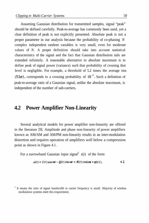
For a narrowband Gaussian input signal2 x(t) of the form:
2 It means the ratio of signal bandwidth to carrier frequency is small. Majority of wirelessmodulation systems meet this requirement.
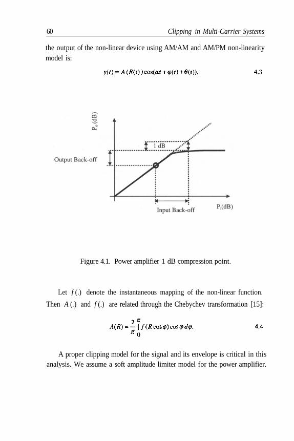
60 Clipping in Multi-Carrier Systems
the output of the non-linear device using AM/AM and AM/PM non-linearitymodel is:
Figure 4.1. Power amplifier 1 dB compression point.
Let f (.) denote the instantaneous mapping of the non-linear function.
Then A (.) and f (.) are related through the Chebychev transformation [15]:
A proper clipping model for the signal and its envelope is critical in thisanalysis. We assume a soft amplitude limiter model for the power amplifier.
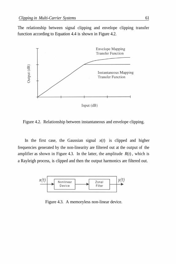
Clipping in Multi-Carrier Systems 61
The relationship between signal clipping and envelope clipping transferfunction according to Equation 4.4 is shown in Figure 4.2.
Figure 4.2. Relationship between instantaneous and envelope clipping.
In the first case, the Gaussian signal x(t) is clipped and higher
frequencies generated by the non-linearity are filtered out at the output of the
amplifier as shown in Figure 4.3. In the latter, the amplitude R(t) , which is
a Rayleigh process, is clipped and then the output harmonics are filtered out.
Figure 4.3. A memoryless non-linear device.

62 Clipping in Multi-Carrier Systems
Statistics of extreme values for Gaussian and Rayleigh processes areessential for understanding and analysis of clipping in multi-carrier systems.Most of the results in this section apply to both Gaussian and Rayleighdistributed random processes [13]. Assume x(t) is a stationary and
continuous with probability one process with finite second order moment.The expected value of number of crossings3 of level l during time period T
by x(t) is [13]
where
and dF(m) is the power spectral density of x(t). Without loss of generality
we assume unity power, The important quantity is the power of
the derivative of x(t).
Rice and others [8, 10] showed that sequences of up-crossings of anergodic and stationary process with continuous sample function withprobability one, asymptotically approaches a Poisson process. For aGaussian signal, the rate of the Poisson process is
3 A random process x(t) has an up-crossing of the level at time if

Clipping in Multi-Carrier Systems 63
The shape of the pulse above level l is a parabolic arc of the form
where duration of clip, is a random variable with Rayleigh probability
density
The above approximation is valid for l >
The envelope of signal R(t) has similar characteristics as a signal x(t)
with twice the bandwidth. Therefore, we assume that the shape of excursionabove level R of the signal envelope is
The excursion pulse is completely characterized by the parameter andsecond order moments of the signal.
4.3 BER Analysis
Usually, the effect of clipping is modelled as an extra additive noise witha variance equal to the energy of clipped portion. This model does notdescribe the instantaneous nature of clipping phenomena as a rare event. Wedefine a conditional bit error rate measure to underline the effect of clippingon bit error rate in a multi-carrier system.
64 Clipping in Multi-Carrier Systems
Defining event A as clipping of the signal above level l, it is clear that
Probability of occurrence of a clipping event during an interval of length
T is and we assume that duration of clipping is short compared to the
OFDM symbol duration. The spectrum of an OFDM signal asymptoticallytends to a rectangular spectrum as the number of carriers increases.
The mean of the corresponding Poisson process is:
where for baseband signal. The expected value of the duration of
the clip is
We use a linear model to show the effect of clipping distortion on the
transmitted signal. The clipped signal is represented as x(t)+ (t) where
the second term includes part of the signal above level l. However, thesecond term is correlated with the signal [8]. The Gram-Schmidt techniquecan be used to de-correlate signal and distortion terms. Defining a newdistortion term as
the signal and distortion terms are non-correlated. However, the second termhas negligible power compared to the first term. The above decompositioncan also be justified by Bussgang’s theorem [14]. For a memoryless non-linear function f(.), Bussgang’s theorem proves that

Clipping in Multi-Carrier Systems 65
Figure 4.4. Memoryless non-linear mapping.
Therefore, we can decompose the output signal into two non-correlatedcomponents:
where x(t) and (t) are “first order” non-correlated .
Using parabolic characteristics of the clipped component, the FourierTransform of the clipped signal will be
This function is shown in Figure 4.5. By using the expected value ofdistortion power in an arbitrary frequency bin we can estimate the overalldistortion effect. The probability distribution function of is
The effect of the noise term in every bin is expected to be increased by
66 Clipping in Multi-Carrier Systems
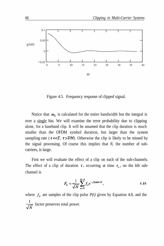
Figure 4.5. Frequency response of clipped signal.
Notice that is calculated for the entire bandwidth but the integral is
over a single bin. We will examine the error probability due to clippingalone, for a baseband clip. It will be assumed that the clip duration is muchsmaller than the OFDM symbol duration, but larger than the systemsampling rate Otherwise the clip is likely to be missed bythe signal processing. Of course this implies that N, the number of sub-carriers, is large.
First we will evaluate the effect of a clip on each of the sub-channels.The effect of a clip of duration occurring at time on the kth sub-
channel is
where are samples of the clip pulse P(t) given by Equation 4.8, and the
factor preserves total power.

Clipping in Multi-Carrier Systems 67
We will replace the discrete Fourier Transform by the conventionalcontinuous one by substituting
where The above approximation is valid because Then
Substituting
where is the pulse spectrum given by 4.16, so that
Since
the response of the lower sub-carriers are approximately equal, with thehigher sub-carriers being progressively reduced.
68 Clipping in Multi-Carrier Systems
The error probability will vary over the sub-carriers. However, theoverall error probability will be dominated by that of the lower sub-carriers,when the constellation sizes are equal, or even more so when the lowerconstellation sizes are larger, as is usual in ADSL. For small k, the responseto a clip of duration in each sub-carrier, will be
where is uniformly distributed on and the Rayleigh probability
distribution of is given by Equation 4.9.
Writing Equation 4.27 as
we wish to find the probability distribution of r.
Using the distribution of given by Equation 4.9,
Substituting
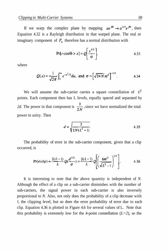
Clipping in Multi-Carrier Systems 69
If we warp the complex plane by mapping thenEquation 4.32 is a Rayleigh distribution in that warped plane. The real or
imaginary component of therefore has a normal distribution with
where
We will assume the sub-carrier carries a square constellation ofpoints. Each component then has L levels, equally spaced and separated by
2d. The power in that component is since we have normalized the total
power to unity. Then
The probability of error in the sub-carrier component, given that a clipoccurred, is
It is interesting to note that the above quantity is independent of N.Although the effect of a clip on a sub-carrier diminishes with the number ofsub-carriers, the signal power in each sub-carrier is also inverselyproportional to N. Also, not only does the probability of a clip decrease withl, the clipping level, but so does the error probability of error due to eachclip. Equation 4.36 is plotted in Figure 4.6 for several values of L. Note thatthis probability is extremely low for the 4-point constellation (L=2), so the
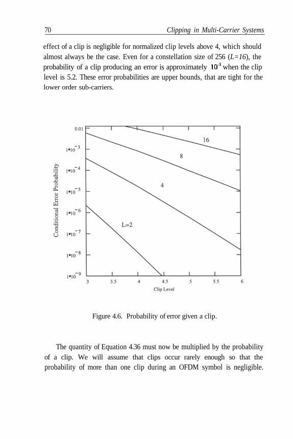
70 Clipping in Multi-Carrier Systems
effect of a clip is negligible for normalized clip levels above 4, which shouldalmost always be the case. Even for a constellation size of 256 (L=16), theprobability of a clip producing an error is approximately when the cliplevel is 5.2. These error probabilities are upper bounds, that are tight for thelower order sub-carriers.
Figure 4.6. Probability of error given a clip.
The quantity of Equation 4.36 must now be multiplied by the probabilityof a clip. We will assume that clips occur rarely enough so that theprobability of more than one clip during an OFDM symbol is negligible.

Clipping in Multi- Carrier Systems 71
Then the probability of a clip, either positive or negative, during a symbolinterval is
so the probability of error is
Figure 4.7. Symbol error probability due to clipping.

72 Clipping in Multi-Carrier Systems
The quantity Pr(e) / N is plotted in Figure 4.7. Again it should be
stressed that this is a lower bound, tight only for low frequency sub-carriers.It is negligibly small for small constellations, and for moderately highclipping levels.
For the case L = 2, which is usual is wireless OFDM systems,
For the case of large constellation size, as occurs in some sub-carriers ofan ADSL system,
The error probability per bit, assuming Gray coded levels in each sub-carrier component, and noting that errors to other than adjacent levels arenegligible, is then
It should be noted that this value holds in the presence of fading,provided that the fading is slow compared to the OFDM symbol rate, and theclip occurs at the transmitter.
If the clip occurs at the transmitter, and additive Gaussian noise ofamplitude n is present on the channel at that time, then the per bit errorprobability in a component of a lower sub-channel when a clip occurs is
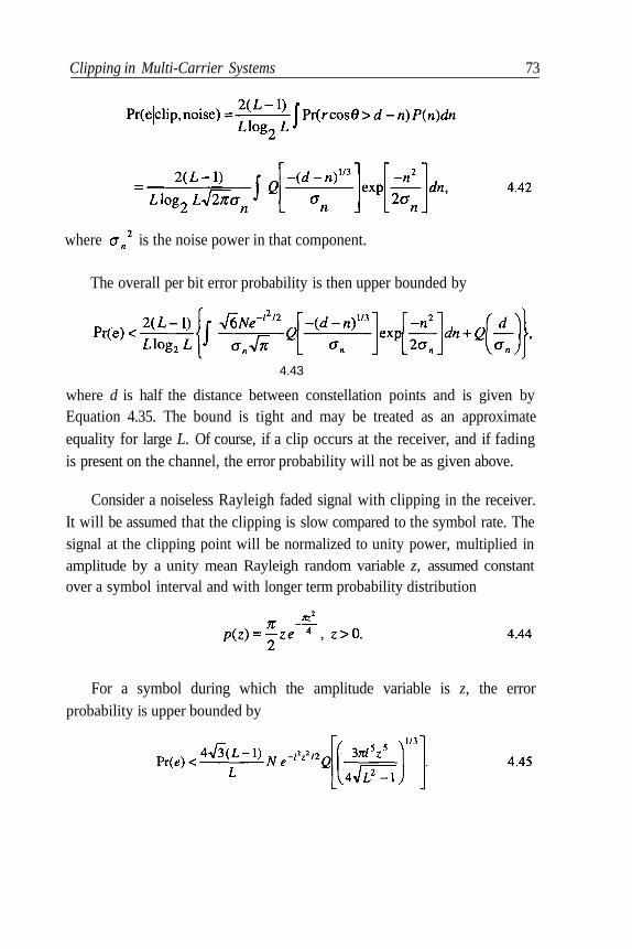
Clipping in Multi-Carrier Systems 73
where is the noise power in that component.
The overall per bit error probability is then upper bounded by
4.43
where d is half the distance between constellation points and is given byEquation 4.35. The bound is tight and may be treated as an approximateequality for large L. Of course, if a clip occurs at the receiver, and if fadingis present on the channel, the error probability will not be as given above.
Consider a noiseless Rayleigh faded signal with clipping in the receiver.It will be assumed that the clipping is slow compared to the symbol rate. Thesignal at the clipping point will be normalized to unity power, multiplied inamplitude by a unity mean Rayleigh random variable z, assumed constantover a symbol interval and with longer term probability distribution
For a symbol during which the amplitude variable is z, the errorprobability is upper bounded by
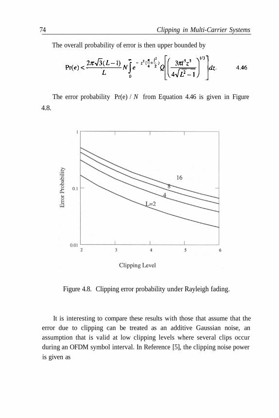
74 Clipping in Multi-Carrier Systems
The overall probability of error is then upper bounded by
The error probability Pr(e) / N from Equation 4.46 is given in Figure
4.8.
Figure 4.8. Clipping error probability under Rayleigh fading.
It is interesting to compare these results with those that assume that theerror due to clipping can be treated as an additive Gaussian noise, anassumption that is valid at low clipping levels where several clips occurduring an OFDM symbol interval. In Reference [5], the clipping noise power
is given as

Clipping in Multi-Carrier Systems 75
where we have normalized that result to unity signal power. This result is
pessimistic in that it does not account for the fact that some of the clippingnoise power is out-of-band. A more accurate expression is given in [6].
For the above Gaussian noise level, the per-symbol error probability for
a sub-carrier is
Figure 4.9. Error probability treating clipping as a Gaussian noise.

This is plotted in Figure 4.9 below. Comparing these calculated errorprobabilities, in particular at a clip level l = 3, with those of Figure 4.7, wecan see that they are much lower even under pessimistic approximations.This is due to the assumption that the noise resulting from clipping is spreaduniformly over time, rather than concentrated as impulses.
4.4 Bandwidth Regrowth
Bandwidth regrowth or out-of-band leakage due to clipping is a critical
issue for wireless communications system designers. The amount of out-of-band spill determines filtering requirements and adjacent channelinterference. Of course analog filtering is also required at the receiver toreduce aliasing. The spectrum of an instantaneously clipped signal has out-of-band band energy at harmonics of the original fundamental band whichreduces the energy of in-band signal. Envelope clipping does not result inany harmonics but the energy spill in the adjacent channel is higher.
Using proper filtering of the power amplifier output mitigates both
effects. However, proper choice of filtering and its feasibility is importantfor overall system performance and cost. Interestingly, filtering of harmonicsresults in higher fluctuation, and therefore, higher peak-to-average ratio in
the received signal.
In this analysis, we use two different approaches to evaluate the impact
of clipping on OFDM signals. The first technique is based on calculation ofthe correlation function of the clipped signal at arbitrary level in order to findthe average power spectral density of the leakage. Secondly, we outline howto take into account the impulsive nature of the leakage.
76 Clipping in Multi-Carrier Systems
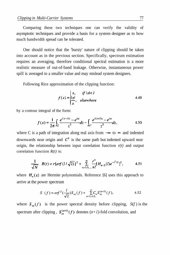
Clipping in Multi-Carrier Systems 77
Comparing these two techniques one can verify the validity ofasymptotic techniques and provide a basis for a system designer as to howmuch bandwidth spread can be tolerated.
One should notice that the 'bursty' nature of clipping should be takeninto account as in the previous section. Specifically, spectrum estimationrequires an averaging, therefore conditional spectral estimation is a morerealistic measure of out-of-band leakage. Otherwise, instantaneous powerspill is averaged to a smaller value and may mislead system designers.
Following Rice approximation of the clipping function:
by a contour integral of the form:
where C is a path of integration along real axis from to and indented
downwards near origin and is the same path but indented upward nearorigin, the relationship between input correlation function r(t) and outputcorrelation function R(t) is:
where are Hermite polynomials. Reference [6] uses this approach to
arrive at the power spectrum
where is the power spectral density before clipping, S(f ) is the
spectrum after clipping , denotes (n+1)-fold convolution, and

78 Clipping in Multi-Carrier Systems
We are interested in evaluating the above in the region where
the undipped spectrum is zero.
In Reference [8], another expression for the power spectrum is given,including high and low frequency asymptotes. In terms of the notation usedin this text, the high frequency asymptotic expression is
The out-of-band spectrum discussed above must be multiplied by the
transmitter filter function The analysis applies when the clipping
level l is low. It is also applicable in any case for determining the long termaverage power spectral density, for example to examine whether the signalmeets regulatory requirements.
In another approach, as shown in the previous section clipping isconsidered as a rare event, hence approaches a Poisson process. We use theapproach outlined in [8] where the random pulse train is
then the spectrum is the expected value of Fourier Transform with respect to
Poisson arrival time and Rayleigh distributed clip duration
Analysis of out-of-band power leakage using the spectrum of clippedsignal amounts to integrating Equation 4.56 over the desired frequency band
Clipping in Multi-Carrier Systems 79
interval. As shown in Figure 4.3 the power amplifier is followed by a filterto control out-of-band leakage. Using the argument presented in the previoussection, we can decompose the clipped signal to two components, theoriginal signal and an non-correlated clipped portion as shown in Equation4.15. Let H(f) denote transfer function of the linear filter representing
cascade of transmit filter, channel, and receive filter. Then, the spectrum of
received signal is
Using the same argument as the previous section, conditional bit errorrate is a more appropriate measure of clipping distortion. To analyze theeffect of clipping on the performance of a receiver using an adjacentchannel, assume another similar OFDM system occupies the adjacent
channel with a guard interval of For example in wireless LAN OFDM
the system channel bandwidth is 100 MHz as shown in Figure 4.10.
The adjacent channel interference due to clipping is
Using the above expression we can calculate conditional errorprobability P(e|clip) by following the same procedure as previous section.
Following the same reasoning used in the last section to evaluate errorprobability, treating the above average leakage power to determine the effecton an adjacent channel may be very optimistic at high clipping level. Asbefore, Equation 4.25 describes the effect of a clip on a sub-channel k, only
we are now interested in an adjacent system so that k > N. That must be
multiplied by the value of the composite filtering function at that sub-
carrier frequency.
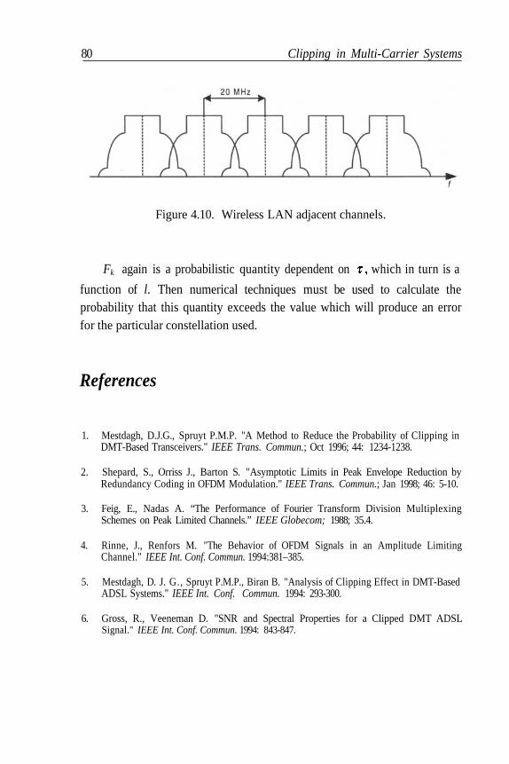
80 Clipping in Multi-Carrier Systems
Figure 4.10. Wireless LAN adjacent channels.
Fk again is a probabilistic quantity dependent on which in turn is a
function of l. Then numerical techniques must be used to calculate theprobability that this quantity exceeds the value which will produce an errorfor the particular constellation used.
References
1. Mestdagh, D.J.G., Spruyt P.M.P. "A Method to Reduce the Probability of Clipping inDMT-Based Transceivers." IEEE Trans. Commun.; Oct 1996; 44: 1234-1238.
2. Shepard, S., Orriss J., Barton S. "Asymptotic Limits in Peak Envelope Reduction byRedundancy Coding in OFDM Modulation." IEEE Trans. Commun.; Jan 1998; 46: 5-10.
3. Feig, E., Nadas A. “The Performance of Fourier Transform Division MultiplexingSchemes on Peak Limited Channels.” IEEE Globecom; 1988; 35.4.
4. Rinne, J., Renfors M. "The Behavior of OFDM Signals in an Amplitude LimitingChannel." IEEE Int. Conf. Commun. 1994:381–385.
5. Mestdagh, D. J. G., Spruyt P.M.P., Biran B. "Analysis of Clipping Effect in DMT-BasedADSL Systems." IEEE Int. Conf. Commun. 1994: 293-300.
6. Gross, R., Veeneman D. "SNR and Spectral Properties for a Clipped DMT ADSLSignal." IEEE Int. Conf. Commun. 1994: 843-847.

Clipping in Multi-Carrier Systems 81
7. VanVleck, J.H., Middletown D. “The Spectrum of Clipped Noise.” Proc. IEEE; Jan1966; 54: 2–19.
8. Mazo, J.E. “Asymptotic Distortion Spectrum of Clipped, DC-Biased, Gaussian Noise.”IEEE Irons. Commun., Aug 1992; COM-40; 8: 1339-1344.
9. Minkoff, J. “The Role of AM-to-PM Conversion in Memoryless Nonlinear Systems."IEEE Trans. Commun., Feb 1985; COM-33; 2: 139-144.
10. Rice, S.O. “Distribution of the Duration of Fades in Radio Transmission.” Bell Syst.Tech. J.; May 1958; 37: 581-635.
11. Kac, M., Slepian D. “Large Excursions of Gaussian Processes.” Ann. Math. Stat.; Dec1959; 30: 1215-1228.
12. Cramer, H., Leadbetter M.R. Stationary and Related Stochastic Processes. New York:Wiley, 1967.
13. Leadbetter, M.R., Lindgren G., Rootzen H. Extremes and Related Properties of RandomSequences and Processes. New York: Springer-Verlag, 1983.
14. Bussgang, J.J. “Crosscorrelation Functions of Amplitude Distorted Gaussian Signals.”Res. Lab. Of Electronics M.I.T., (Cambridge, Mass.) Tech. Rep; Mar 26, 1952; 216:3.
15. Blachman, N.M. “Detectors, Bandpass Non-Linearities, and Their Optimization:Inversion of the Chebyshev Transform.” IEEE Trans. Inform. Theory, Jul 1971; IT-17:398-404.
Chapter 5 Synchronization
Multi-carrier modems, like any other digital communication modems,require a reliable synchronization scheme. Parallel transmission of Nsymbols results in a longer symbol duration, consequently there is lesssensitivity to the timing offset. In other words, unlike single carrier systemsin which a timing jitter can create inter-symbol interference, it does notviolate orthogonality of transmitted waveforms in a multi-carrier system.However, frequency offset is detrimental to OFDM systems and has animportant role in system design. Phase noise is another critical impairment in
wireless OFDM.
In this chapter we will review the effect of timing and frequency jitter inOFDM, and discuss some of the synchronization techniques.
5.1 Timing and Frequency Offset in OFDM
Assuming that interference between OFDM blocks is negligible, a
transmitted OFDM signal can be represented as
83

84 Synchronization
where and are pre-and postfix lengths, and w(t) is the time domain
window function. The received signal r(t) is filtered and sampled at the rate
of multiples of 1/T.
The sampled signal at the output of the receiver FFT with ideal channelcan be represented as
where is the Fourier Transform of the periodically repeated analog
equivalent of the signal generated by transmitter's IFFT. Therefore,
is a line spectrum at and W(f) is the Fourier Transform of window
function w(t).
Assuming that the sampling time has a relative phase offset of and theoffset does not change during one OFDM symbol, the sampled receivedsignal for a non-dispersive channel can be simplified to:
where represents envelope delay distortion. After the Fourier Transform
at the receiver,
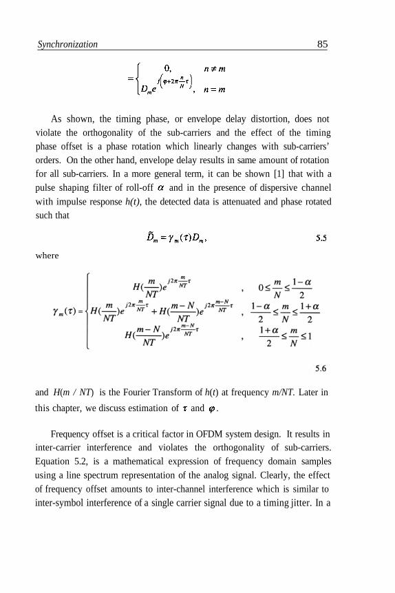
Synchronization 85
As shown, the timing phase, or envelope delay distortion, does notviolate the orthogonality of the sub-carriers and the effect of the timingphase offset is a phase rotation which linearly changes with sub-carriers’orders. On the other hand, envelope delay results in same amount of rotationfor all sub-carriers. In a more general term, it can be shown [1] that with apulse shaping filter of roll-off and in the presence of dispersive channel
with impulse response h(t), the detected data is attenuated and phase rotatedsuch that
where
and H(m / NT) is the Fourier Transform of h(t) at frequency m/NT. Later in
this chapter, we discuss estimation of and .
Frequency offset is a critical factor in OFDM system design. It results ininter-carrier interference and violates the orthogonality of sub-carriers.Equation 5.2, is a mathematical expression of frequency domain samplesusing a line spectrum representation of the analog signal. Clearly, the effectof frequency offset amounts to inter-channel interference which is similar tointer-symbol interference of a single carrier signal due to a timing jitter. In a

86 Synchronization
non-dispersive channel with rectangular pulse shaping, the interferencecaused by frequency offset could be too constraining. The sampled signal is
After DFT we have
where
is the relative frequency deviation. As Equation 5.8 shows, In addition toattenuation of desied signal, there is an interference between differentsymbols of several sub-carriers. This effect creates a significant ICI and isone of the important impairments in OFDM systems, as shown in Figure 5.1.The second term represents the interference from other sub-carriers which isdual to ISI in time domain due to timing offset.
In order to avoid ICI caused by frequency offset, the window function
must be such that zero crossings of its Fourier Transform are at multiples ofsymbol frequency.

Synchronization 87
A generalized sinc function of the form
for any differentiable function, g(t) satisfies the condition of Equation 5.11.
Another desired property of a sinc function is its low rate of change in thevicinity of sampling points in frequency. One common choice is a raisedcosine function in time
where is the roll-off factor for time domain pulse shaping. Notice that a
higher roll-off factor requires a longer cyclic extension and guard interval,which consumes higher bandwidth.
Sensitivity of OFDM systems to frequency offset is sometimes tooconstraining. Therefore, in practice, the zero ICI condition is partly relaxedto provide more robustness against frequency offset. In other words, wetolerate a small amount of ISI at the cost of much less ICI. A Gaussianwindow is one example in which a single parameter adjustment can controlthe ISI and ICI trade-off.
The effect of frequency offset on ICI is depicted in Figure 5.1. As shown,proper windowing has a significant impact on the sensitivity of the receiverto frequency offset. A reasonable design technique is to target an acceptablefrequency offset and choose a proper window.

88 Synchronization
Figure 5.1. ACI caused by frequency offset.
5.2 Synchronization and System Architecture
A synchronization sequence in an OFDM system is shown in Figure 5.2.
Figure 5.2. Synchronization sequence in OFDM.
Synchronization 89
Initially, a coarse frame (or packet) synchronization is required to providetiming information regarding the OFDM symbol. Then, a frequencycorrection prior to FFT is implemented to reduce the effect of inter-channelinterference. Consequently, further stages of fine timing and frequency offsetare implemented. These may be combined in a joint estimation block. Ingeneral, frame timing and frequency correction are more complicated andrequire higher hardware/software resources. Timing and frequencycorrection techniques for OFDM can be classified into two categories: data-aided and non-linear techniques. Data aided techniques use a known bit
pattern or pilot signal to estimate the timing or frequency offset. Non-lineartechniques utilize the cyclostationarity characteristics of the signal to extract
the desired harmonic component by using a non-linear operation. Use ofdata-aided techniques is applicable to many OFDM digital communicationsystems such as HDTV and Wireless LAN. Pilot signal fields are providedin existing standards.
5.3 Timing and Frame Synchronization
Initially a frame (packet or slot) synchronization circuit is required todetect the frame starting point. This is usually achieved by correlating the
incoming signal with a known preamble. The same circuit is sometimes usedto adjust for initial gain control. Therefore, the threshold of the detectioncircuit should be adjusted accordingly. A general block diagram is shown inFigure 5.3. Since timing offset does not violate orthogonality of the symbolsit can be compensated after the receiver FFT.

Figure 5.3. Frame synchronization.
As shown in Equation 5.8, the effect of the timing offset is a phaserotation which linearly increases with sub-carrier order. In order to estimate
the timing offset, we should solve a regression problem with properweighting to represent the effect of fading in the channel.
Figure 5.4. Timing offset estimate.
Frequency offset estimation in packet data communications requires fast
acquisition. Hence, phase-lock techniques are not applicable for initial
90 Synchronization

coarse correction. For this purpose, a pilot or training sequence should be
transmitted. This can be achieved by sending a pilot in one or two bins and
estimate the frequency offset by measuring the energy spread in other bins,or by using a training sequence or pilot in every bin and measuring the phasedifference by repeating the same pattern. Usually, the second approach ismore reliable, as additive noises in different bins are independent and theestimate convergence will be faster. In the following, we discuss bothtechniques and compare the result analytically and through simulation.
5.4 Frequency Offset Estimation
Frequency offset should be corrected before the receiver FFT. The FFTcan be used as a frequency offset detector. Before correction for frequencyoffset, C/I will not be at the acceptable level for reliable data transmission.Therefore, It is preferrable that entire bins should be used for frequencyestimation purposes initially. We assume a known data pattern is used forsynchronization. After FFT, at the receiver, we have:
If the same block is repeated, the result would be
Therefore, we can obtain a proper estimate of by averaging the
product of every bin from one symbol and the same bin from the previoussymbol, and then averaging the result.
Synchronization 91

92
This process is shown in Figure 5.5:
Figure 5.5. Frequency offset estimation.
The number of repetitions depends on the signal-to-noise ratio and therequired accuracy of frequency estimation. Double averaging accelerates theconvergence of the estimate significantly. This scheme works in low signal-to-noise ratios as well. However, this technique is limited to frequency offsetof less than The initial frequency offset could be higher than
that limit, and requires an initial coarse acquisition. A typical coarsefrequency detection in single and multi-carrier systems is the MaximumLikelihood estimation technique.
A digital implementation of the technique is shown in the Figure 5.6where denotes a matched filter tuned to transmit filter impulse
response shifted by frequency offset of
Synchronization

Figure 5.6. A digital implementation of coarse frequency offset estimationusing maximum likelihood criteria.
5.5 Phase Noise
Effects of Phase Noise
Intermediate stages of modulation, such as between RF and IF, canintroduce degradation due not only to frequency error as describedpreviously, but also to phase noise in the local oscillators involved in suchmodulation. Phase noise is the zero mean random process of the deviation of
the oscillator's phase from a purely periodic function at the averagefrequency. The oscillator output may be considered to be an ideal sine wavephase modulated by the random process. The power spectral density isgenerally normalized to the power of the sine wave. Higher quality (andmore costly) oscillators will typically have lower phase noise than cheaperones. Therefore, one may expect greater phase noise at the mobile set in awireless system, as opposed to the base station, and similarly in the customer
Synchronization 93
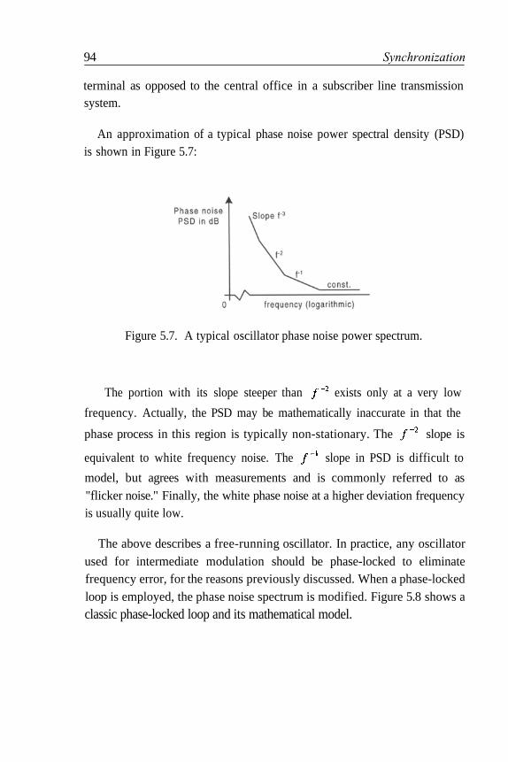
94 Synchronization
terminal as opposed to the central office in a subscriber line transmissionsystem.
An approximation of a typical phase noise power spectral density (PSD)is shown in Figure 5.7:
Figure 5.7. A typical oscillator phase noise power spectrum.
The portion with its slope steeper than exists only at a very low
frequency. Actually, the PSD may be mathematically inaccurate in that the
phase process in this region is typically non-stationary. The slope is
equivalent to white frequency noise. The slope in PSD is difficult to
model, but agrees with measurements and is commonly referred to as"flicker noise." Finally, the white phase noise at a higher deviation frequencyis usually quite low.
The above describes a free-running oscillator. In practice, any oscillatorused for intermediate modulation should be phase-locked to eliminatefrequency error, for the reasons previously discussed. When a phase-lockedloop is employed, the phase noise spectrum is modified. Figure 5.8 shows aclassic phase-locked loop and its mathematical model.

Figure 5.8. Classical phase-locked loop.
The variables are phase deviations from nominal. and are
the input, output, and internal oscillator phase deviations respectively. Thelow-pass filter F(s) must be chosen such that the feedback loop is stable. Thevoltage-controlled oscillator (VCO) has an output frequency deviation fromits nominal value that is proportional to the control voltage. Since phase isthe integral of frequency, the transfer function of the VCO is K/s as shown.The equation of the loop is
Because the open loop transfer function has a pole at zero frequency, thefrequency of the VCO will lock exactly to the average input frequency,provided the initial frequency difference is within the lock-in range of theloop. Substituting the frequency variable for the LaPlace variable s, the
power transfer function is
Synchronization 95
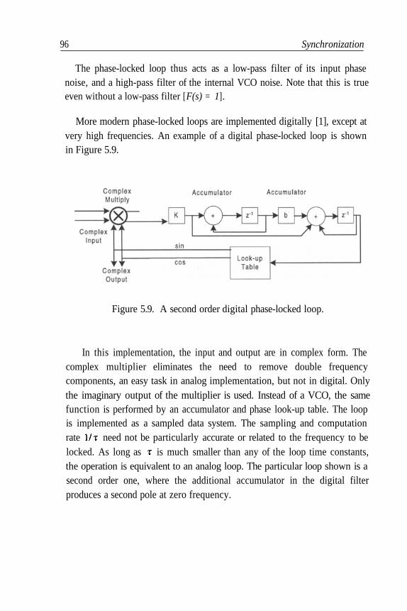
The phase-locked loop thus acts as a low-pass filter of its input phasenoise, and a high-pass filter of the internal VCO noise. Note that this is trueeven without a low-pass filter [F(s) = 1].
More modern phase-locked loops are implemented digitally [1], except atvery high frequencies. An example of a digital phase-locked loop is shownin Figure 5.9.
Figure 5.9. A second order digital phase-locked loop.
In this implementation, the input and output are in complex form. Thecomplex multiplier eliminates the need to remove double frequencycomponents, an easy task in analog implementation, but not in digital. Onlythe imaginary output of the multiplier is used. Instead of a VCO, the samefunction is performed by an accumulator and phase look-up table. The loopis implemented as a sampled data system. The sampling and computationrate need not be particularly accurate or related to the frequency to belocked. As long as is much smaller than any of the loop time constants,the operation is equivalent to an analog loop. The particular loop shown is asecond order one, where the additional accumulator in the digital filterproduces a second pole at zero frequency.
96 Synchronization
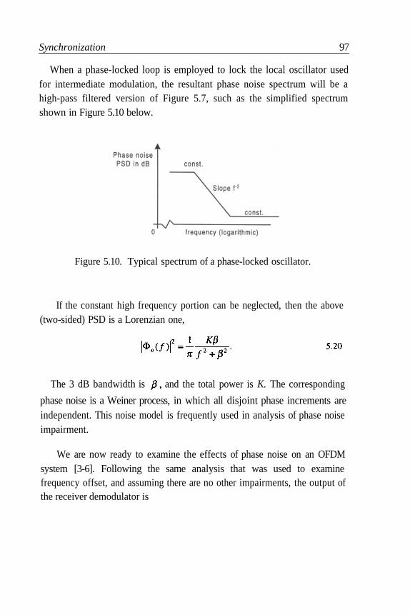
When a phase-locked loop is employed to lock the local oscillator usedfor intermediate modulation, the resultant phase noise spectrum will be ahigh-pass filtered version of Figure 5.7, such as the simplified spectrumshown in Figure 5.10 below.
Figure 5.10. Typical spectrum of a phase-locked oscillator.
If the constant high frequency portion can be neglected, then the above(two-sided) PSD is a Lorenzian one,
The 3 dB bandwidth is and the total power is K. The corresponding
phase noise is a Weiner process, in which all disjoint phase increments areindependent. This noise model is frequently used in analysis of phase noiseimpairment.
We are now ready to examine the effects of phase noise on an OFDMsystem [3-6]. Following the same analysis that was used to examinefrequency offset, and assuming there are no other impairments, the output ofthe receiver demodulator is
Synchronization 97
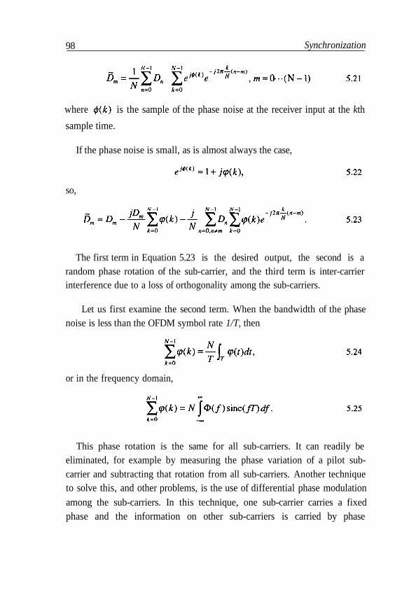
98
where is the sample of the phase noise at the receiver input at the kth
sample time.
If the phase noise is small, as is almost always the case,
so,
The first term in Equation 5.23 is the desired output, the second is arandom phase rotation of the sub-carrier, and the third term is inter-carrierinterference due to a loss of orthogonality among the sub-carriers.
Let us first examine the second term. When the bandwidth of the phasenoise is less than the OFDM symbol rate 1/T, then
or in the frequency domain,
This phase rotation is the same for all sub-carriers. It can readily beeliminated, for example by measuring the phase variation of a pilot sub-carrier and subtracting that rotation from all sub-carriers. Another techniqueto solve this, and other problems, is the use of differential phase modulationamong the sub-carriers. In this technique, one sub-carrier carries a fixedphase and the information on other sub-carriers is carried by phase
Synchronization

differences. This is applicable only to constellations of constant amplitude.Furthermore, there is a noise performance penalty when compared withcoherent demodulation.
If the above correction is performed, we are left with the inter-carrier
interference. Again, assuming the phase noise bandlimited to less than 1/T,that interference is
If the data symbols on the different sub-carriers are independent, thenthe interference may be treated as a Gaussian noise of power
where is the average power of the nth sub-carrier. For any phase noise
PSD that is decreasing with frequency, near sub-carriers will contributegreater to this interference than sub-carriers further removed from the sub-carrier of interest. For this reason, sub-carriers near the center of thefrequency band will be subject to more interference than sub-carriers at theband edge by up to a factor of two. More importantly, the interferenceincreases as the spacing between sub-carriers decreases.
The noise-to-signal ratio for a sub-carrier near the middle of the band,assuming equal power on all sub-carriers, is
Synchronization 99

100 Synchronization
For the Lorenzian noise spectrum given previously, this quantity is plotted
as a function of in Figure 5.11, normalized by the ratio of phase noise
power to power in the sub-carrier. Here, all sub-carrier powers were assumed
to be equal. Note that is the ratio of the 3 dB bandwidth of the phase
noise to the OFDM symbol rate. To find the un-normalized noise-to-signalratio, the plotted quantity should be multiplied by the phase noise to sub-carrier power ratio.
Figure 5.11. Inter-carrier interference noise.
It is seen that as long as the OFDM symbol rate is greater thanapproximately twice the phase noise bandwidth, the performance degradesas that symbol rate, or, equivalently, the sub-carrier spacing, decreases.Therefore, under these conditions, the use of a large number of sub-carriersto carry a given bit rate is detrimental. However when the OFDM symbolrate increases beyond approximately twice the phase noise bandwidth, there
Synchronization 101
is little further degradation., assuming that the line rate is still much greaterthan the noise bandwidth.
Another form of phase noise that can exist even in OFDM systemswithout intermediate modulations, such as in wireline applications, resultsfrom jitter in the sampling time at the receiver input. In Reference [7], it isshown that when the timing jitter is constant over an OFDM symbol interval,no inter-carrier interference results. In this case, each sub-carrierconstellation is subjected to rotation proportional to the timing offset and tothe frequency of that sub-carrier.
References
1. Pollet, T., Moeneclay M. "Synchronizability of OFDM Signals." IEEE Proc. of GlobalTelecom Conf. (GLOBECOM '95); Nov 1995; 3: 2054-2058.
2. Lindsay, W.C., Chie C.M. "A Survey of Digital Phase-Locked Loops." Proc. IEEE; Apr1981; 9; 4: 410-431.
3. Pollet, T., VanBladel M., Moeneclay M. "BER Sensitivity of OFDM Systems to CarrierFrequency Offset and Wiener Phase Noise." IEEE Trans. Commun.; Feb/Mar/Apr 1995;43; 2/3/4: 191-193.
4. Robertson, P., Kaiser S. "Analysis of the Effects of Phase Noise in OFDM Systems."IEEE Int. Conf. Commun.; 1995: 1652-1657.
5. Armada, G., Calvo M. "Phase Noise and Sub-Carrier Spacing Effects on thePerformance of an OFDM Communication System." IEEE Commun. Letters; Jan 1998;2; 1: 11-13.
6. Steendam, H., Moeneclay M., Sari H. "The Effects of Carrier Phase Jitter on thePerformance of Orthogonal Frequency Division Multiple Access Systems." IEEE Trans.Commun.; Apr 1998; 46; 4: 456-459.
7. Zogakis, T.N., Cioffi J.M. "The Effect of Timing Jitter on the Performance of a DiscreteMultitone System." IEEE Trans. Commun.; Jul 1996; 44; 7: 799-808.
Chapter 6 Equalization
6.1 Introduction
One of the advantages of a multi-carrier system is its robustness against
inter-symbol interference. The longer duration of OFDM symbols provideshigher immunity against delay spread and ISI. As long as channel dispersion
is not longer than the OFDM symbol guard interval, system performance
does not degrade due to ISI and use of time domain equalization is notusually mandated.
However, in case of higher data rates and channels with extensive time
dispersion an equalizer is unavoidable. Albeit, the structure of the equalizer
is different from that of single carrier systems. The purpose of equalization is
not complete removal but restriction of inter-symbol interference to a
tolerable extent.
Frequency domain equalization, in the absence of inter-channel
interference (ICI) is used to compensate for channel complex gain at each
sub-carrier frequency. Using time-frequency duality, complex gain
103
104 Equalization
compensation after FFT is equivalent to a convolution of a FIR filter in timedomain (residual equalization).
In this chapter, we review main differences of equalization in single and
multi-carrier and follow up with analytical and practical aspects of timedomain equalization. Then, frequency domain equalization and echo
cancellation are discussed in sections 3 and 4. Using duality prniciple, we
present a unified approach to time and frequency domain equalization.
6.2 Time Domain Equalization
A brief review of decision feedback equalizer structure and performanceshould help the reader to readily understand the analysis and design ofequalizers for multi-carrier.
Decision Feedback Equalizers
In a decision feedback equalizer, the forward filter whitens the noise andproduces a response with post-cursor ISI only, and the feedback filter thencancels that post-cursor ISI. The optimum forward filter for a zero-forcingDFE can be considered as cascade of a matched filter followed by a linearequalizer and a causal whitening filter whose transfer function can be foundby spectral factorization of the channel power spectrum. The forward filter,
therefore, first minimizes ISI, then noise power at the input of slicer,reintroducing causal ISI. Notice that the separation and ordering has onlyanalytic significance [4]. In practice, all forward filters are usually lumpedtogether in one adaptive filter.
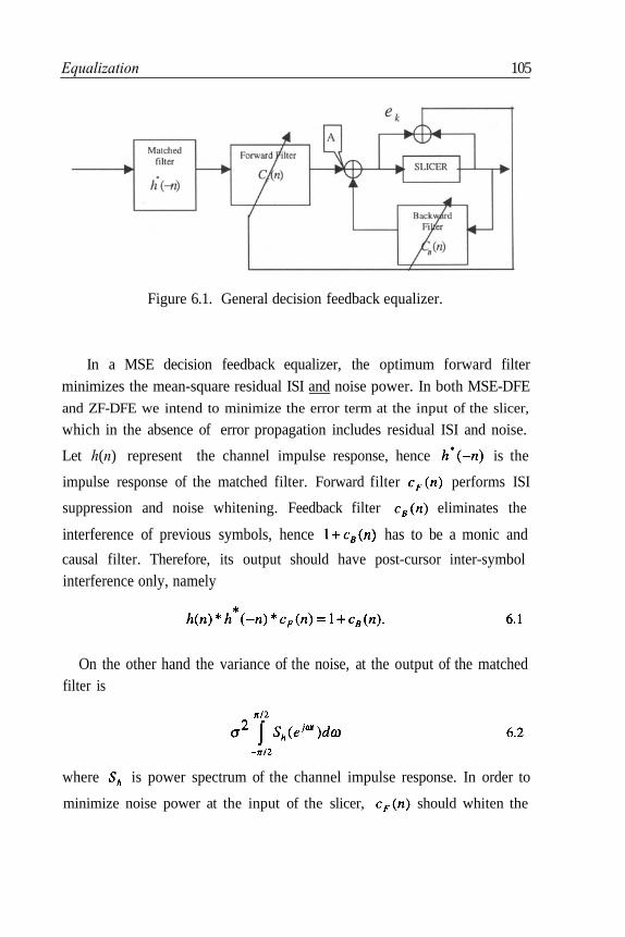
Equalization 105
Figure 6.1. General decision feedback equalizer.
In a MSE decision feedback equalizer, the optimum forward filterminimizes the mean-square residual ISI and noise power. In both MSE-DFEand ZF-DFE we intend to minimize the error term at the input of the slicer,
which in the absence of error propagation includes residual ISI and noise.
Let h(n) represent the channel impulse response, hence is the
impulse response of the matched filter. Forward filter performs ISI
suppression and noise whitening. Feedback filter eliminates the
interference of previous symbols, hence has to be a monic and
causal filter. Therefore, its output should have post-cursor inter-symbolinterference only, namely
On the other hand the variance of the noise, at the output of the matchedfilter is
where is power spectrum of the channel impulse response. In order to
minimize noise power at the input of the slicer, should whiten the

106 Equalization
noise. Rewriting Equation 6.1 in the frequency domain, the forward filtertransfer function is
The forward filter may apply further linear transformation to the inputsignal to meet some optimality criteria such as minimizing square error or
peak distortion. To whiten a stochastic process with spectrum of it
should satisfy the following equation:
Since
from Equation 6.4 we have:
The same procedure [4] can be followed for the MSE equalizer to obtain
In the following, we discuss some important issues about the DFE withfinite tap FIR feedback and forward filters as a preface for futurediscussions.
The input to the feedback filter is noise free, therefore the feedback filtereliminates the post-cursor ISI both in ZF-DFE and MSE-DFE. The errorterm used for training is memoryless and defined as:
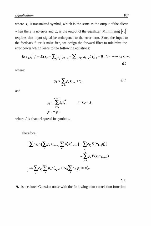
Equalization 107
where is transmitted symbol, which is the same as the output of the slicer
when there is no error and is the output of the equalizer. Minimizing
requires that input signal be orthogonal to the error term. Since the input tothe feedback filter is noise free, we design the forward filter to minimize theerror power which leads to the following equations:
where:
and
where l is channel spread in symbols.
Therefore,
is a colored Gaussian noise with the following auto-correlation function

108 Equalization
The solution to equation 6.9 is
where
N is the number of forward taps and
Coefficients of the backward filter can be found by
where
The forward filter is anti-causal which means that the main tap is
assumed to be the closest one to the slicer. The forward taps should removethe entire post-cursor. Practically, the matched filter is usually absorbed inthe forward equalizer4 then h replaces p is Equations 6.12 and 6.16. Notice
that the feedback filter is designed to minimize the post-cursor ISI at theinput of the slicer. In practice, and are adjusted adaptively.
4 We can interpret this as replacing the matched filter with a whitening matched filter
Equalization 109
6.3 Equalization in DMT
Multi-carrier systems are robust against inter-symbol interference aslong as orthogonality of adjacent symbols is preserved in the frequencydomain. In other words, the symbol duration of the OFDM signal isextended to beyond T. However, if channel impulse response spread is morethan the prefix extension, inter-symbol interference can degrade theperformance.
There are several fundamental differences between time domainequalization requirements of OFDM channels and classic decision feedbackequalizers:
a) An equalizer of an OFDM system does not need to cancel the ISI
entirely but to limit its length. Unlike a single carrier system in whichequalization minimizes ISI, we only need to reduce it to a time span lessthan the length of guard interval.
b) The channel impulse response is modelled as an ARMA system.Usually, the channel impulse response is too long. Therefore, a model of
the form
is appropriate.
c) The equalizer does not work as a DFE in data mode. Unless channelcharacteristics change rapidly, equalizer taps are adjusted during thetraining sequence and the same tap values are preserved during data
mode.
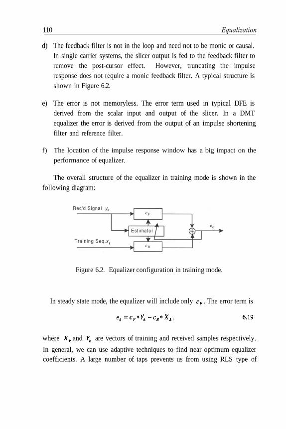
110 Equalization
d) The feedback filter is not in the loop and need not to be monic or causal.In single carrier systems, the slicer output is fed to the feedback filter toremove the post-cursor effect. However, truncating the impulseresponse does not require a monic feedback filter. A typical structure isshown in Figure 6.2.
e) The error is not memoryless. The error term used in typical DFE isderived from the scalar input and output of the slicer. In a DMTequalizer the error is derived from the output of an impulse shorteningfilter and reference filter.
f) The location of the impulse response window has a big impact on the
performance of equalizer.
The overall structure of the equalizer in training mode is shown in the
following diagram:
Figure 6.2. Equalizer configuration in training mode.
In steady state mode, the equalizer will include only The error term is
where and are vectors of training and received samples respectively.
In general, we can use adaptive techniques to find near optimum equalizercoefficients. A large number of taps prevents us from using RLS type of

Equalization 111
algorithms. On the other hand, a wide spread of eigenvalues of the inputsignal covariance matrix can slow down convergence of the equalizer. Adifferent technique for equalizer tap adjustment is based on linear predictiontheory as explained below.
During acquisition, the frame is repeated and can be used for equalizertraining. In this approach, we use second order statistics of the channel toproduce a one shot estimate of equalizer coefficients. In order to use thepredictor format of linear regression techniques, without loss of generality,assume is monic. So, the predictor format is:
where
and,
The least square solution of linear regression is:
with:
where
and
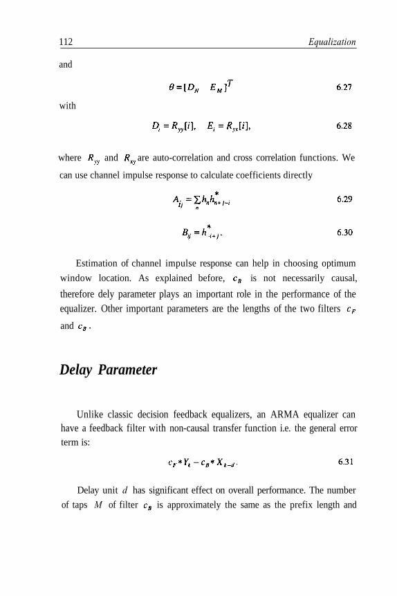
112 Equalization
and
with
where and are auto-correlation and cross correlation functions. We
can use channel impulse response to calculate coefficients directly
Estimation of channel impulse response can help in choosing optimum
window location. As explained before, is not necessarily causal,
therefore dely parameter plays an important role in the performance of theequalizer. Other important parameters are the lengths of the two filters
and
Delay Parameter
Unlike classic decision feedback equalizers, an ARMA equalizer canhave a feedback filter with non-causal transfer function i.e. the general errorterm is:
Delay unit d has significant effect on overall performance. The number
of taps M of filter is approximately the same as the prefix length and

Equalization 113
number of taps for the forward filter The delay unit should be
chosen properly to capture the most significant window of the impulseresponse. Brute force trial and error is one option. A more intelligenttechnique can use the estimate of the impulse response to pick a properstarting point where the energy of the impulse response is above a threshold.The threshold should be the ratio of tap power to overall window power.Since the length of the window function and forward equalizer should be asshort as possible, proper choice of starting point is of significant importance.In other words, in an ARMA model the number of zeroes is not assignedproperly.
AR Approximation of ARMA Model
Direct solution of Equation 6.23 requires a non-Toeplitz matrixinversion and is numerically sensitive and intensive. One technique toalleviate the numerical difficulty of least square solution is by usingtechniques for AR approximation of the channel response ARMA model,which results in a numerically attractive Toeplitz correlation matrix. Adescription of embedding techniques is presented in the Appendix. In thefollowing, the procedure for this analysis is briefly described.
By using embedding techniques, as explained in the Appendix, theARMA model of Equation 6.18 is approximated by a two-channel ARmodel.
If the covariance matrix is available the problem can be reduced tosolution of a normal (Yule-Walker) equation. The multi-channel version ofthe Levinson algorithm is a computationally efficient solution for the two-channel AR model at hand. As a reference, the recursive technique ispresented here:

114 Equalization
Initialization:
where
is the j-th forward prediction coefficient of two-channel model at i-th
iteration and is the j-th backward prediction coefficient at i-th
iteration and
If the input signal x is white then
with
Recursion:

Equalization 115
where the reflection coefficients are,
Figure 6.3 shows the structure of an equalizer using a lattice filter. Thisstructure represents the case of equal number of poles and zeros. Theextension to unequal number of poles and zeroes is straightforward andexplained in [5].
Figure 6.3. Equalization using order update.
The above approach is convenient for batch or frame based processingwhere the entire frame is buffered and processed for equalization. Instead ofinverting the large matrix of Equation 6.13 for example, this structure can beused in the training mode of an ADSL receiver. This technique can be
116 Equalization
implemented iteratively in time and order when the covariance is not knownin advance. The time/order updating algorithm increases the order whileupdating the coefficients of the equalizer. In some cases, we can preservethe order and continue updating the parameters using adaptive techniques.This technique is useful when the delay profile of the channel does notchange significantly but some slow adaptation improves the performance.
6.4 Frequency Domain Equalization
Once it is assured that orthogonality of the sub-carriers is maintained,possibly through the use of the cyclic prefix and time domain equalization aspreviously discussed, then the final frequency domain equalization of anOFDM signal is an extremely simple process. This is certainly one of the
key advantages of OFDM.
After demodulation, the sub-carriers will be subjected to different lossesand phase shifts, but there will be no interaction among them. Frequencydomain equalization therefore consists solely of separate adjustments of sub-carrier gain and phase, or equivalently of adjusting the individual decisionregions. For the case where the constellations consist of equal amplitudepoints, as in PSK, this equalization becomes even simpler in that only phaseneed be corrected for each sub-carrier, because amplitude has no effect on
decisions.
A simplified picture of the place of frequency domain equalization isshown in Figure 6.4, where the equalizer consists of the set of complexmultipliers, {A}, one for each sub-carrier.
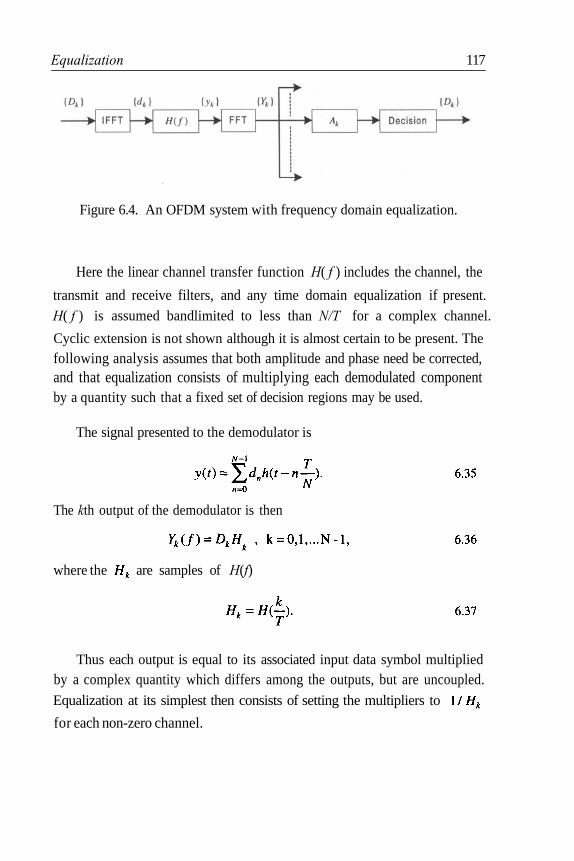
Equalization 117
Figure 6.4. An OFDM system with frequency domain equalization.
Here the linear channel transfer function H( f ) includes the channel, the
transmit and receive filters, and any time domain equalization if present.H( f ) is assumed bandlimited to less than N/T for a complex channel.
Cyclic extension is not shown although it is almost certain to be present. Thefollowing analysis assumes that both amplitude and phase need be corrected,and that equalization consists of multiplying each demodulated componentby a quantity such that a fixed set of decision regions may be used.
The signal presented to the demodulator is
The kth output of the demodulator is then
where the are samples of H(f)
Thus each output is equal to its associated input data symbol multipliedby a complex quantity which differs among the outputs, but are uncoupled.Equalization at its simplest then consists of setting the multipliers to
for each non-zero channel.

118 Equalization
The above approach is optimum in every sense under high signal-to-noise conditions. It also produces minimum probability of error at any noise
level, and is an unbiased estimator of the input data However if the
criterion to be optimized is minimum mean-square error particularly, thenthe optimum multipliers are modified to
where is the noise power in the demodulated sub-channel. However this
value produces a biased estimator and does not minimize error probability.
As a practical implementation issue, for variable amplitudeconstellations, it is frequently desirable to have a fixed grid of decision
regions. The s can then be scaled in amplitude such that the separation of
constellation points is constant.
Since a shift in timing phase is equivalent to a phase shift
frequency domain equalization readily corrects for such timing shift.
In principle frequency domain equalization could be employed whenorthogonality is lost due to interference among OFDM symbols. In this case,rather than a simple multiplier per sub-channel, a matrix multiplicationwould be required. This approach is bound to require more computationalload than the combination of time and frequency domain equalizers.
During system initialization, any time domain equalizer must be adjustedbefore frequency domain equalization is performed. Then any periodic testsignal with full frequency content, such as a repeated segment of a PNsequence without cyclic prefix, may be used to adapt the frequency domainequalizer. The demodulator outputs should be averaged over many periods to
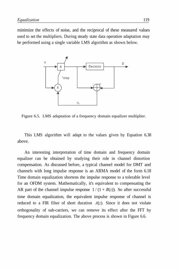
Equalization 119
minimize the effects of noise, and the reciprocal of these measured valuesused to set the multipliers. During steady state data operation adaptation maybe performed using a single variable LMS algorithm as shown below.
Figure 6.5. LMS adaptation of a frequency domain equalizer multiplier.
This LMS algorithm will adapt to the values given by Equation 6.38
above.
An interesting interpretation of time domain and frequency domainequalizer can be obtained by studying their role in channel distortioncompensation. As discussed before, a typical channel model for DMT andchannels with long impulse response is an ARMA model of the form 6.18Time domain equalization shortens the impulse response to a tolerable levelfor an OFDM system. Mathematically, it's equivalent to compensating theAR part of the channel impulse response 1 / (1 + B(z)). So after successful
time domain equalization, the equivalent impulse response of channel isreduced to a FIR filter of short duration A(z). Since it does not violate
orthogonality of sub-carriers, we can remove its effect after the FFT byfrequency domain equalization. The above process is shown in Figure 6.6.
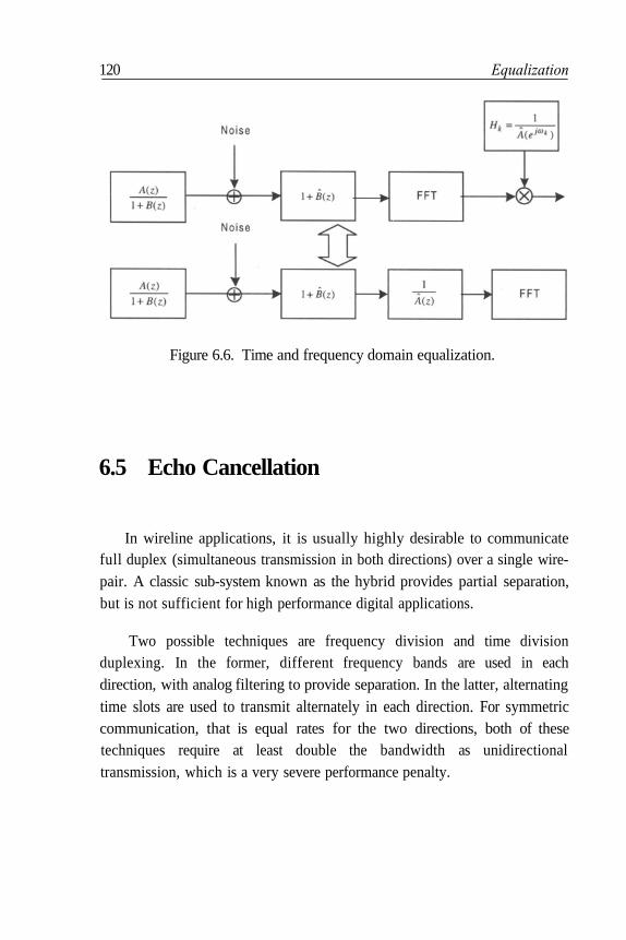
120 Equalization
Figure 6.6. Time and frequency domain equalization.
6.5 Echo Cancellation
In wireline applications, it is usually highly desirable to communicatefull duplex (simultaneous transmission in both directions) over a single wire-pair. A classic sub-system known as the hybrid provides partial separation,but is not sufficient for high performance digital applications.
Two possible techniques are frequency division and time divisionduplexing. In the former, different frequency bands are used in eachdirection, with analog filtering to provide separation. In the latter, alternating
time slots are used to transmit alternately in each direction. For symmetriccommunication, that is equal rates for the two directions, both of thesetechniques require at least double the bandwidth as unidirectionaltransmission, which is a very severe performance penalty.

Equalization 121
Far preferable is the technique of echo cancellation, where at each endthe leakage of transmitted signal into the co-located receiver is cancelled bycreating and subtracting a replica of that leakage. The precision required is
quite high, as illustrated in the example of a bad case wireline system shownin Figure 6.7.
Figure 6.7. An example system illustrating echo cancellation requirement.
In this example, the loss of the line is 40 dB. while the hybrid providesonly 15 dB of loss. The leakage of the transmitted signal, or "echo", istherefore 25 dB higher than the desired received signal. One consequence isthat the level which the front end of the receiver, in particular the A/D
converter, must accommodate is dominated by the echo rather than thereceived signal. Of more interest here is the high degree of echo cancellationrequired. Assume, as in the figure, that a signal-to noise ratio of 30 dB isrequired, and that uncancelled echo can be treated as noise. If we use thereasonable design rule that the uncancelled echo should be at least 10 dBbelow the line noise, thereby increasing the noise by less than 0.4 dB, thelevel of the uncancelled echo must be below -80 dB. Because the hybridprovides only 15 dB of reduction, the echo canceller must provide an
additional 65 dB of rejection. This requirement is far more severe than thatof equalization, so that a much greater arithmetic precision and number of
taps is required.
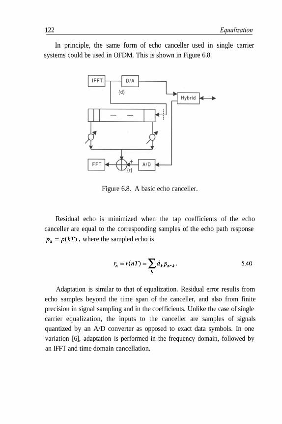
122 Equalization
In principle, the same form of echo canceller used in single carriersystems could be used in OFDM. This is shown in Figure 6.8.
Figure 6.8. A basic echo canceller.
Residual echo is minimized when the tap coefficients of the echocanceller are equal to the corresponding samples of the echo path response
where the sampled echo is
Adaptation is similar to that of equalization. Residual error results fromecho samples beyond the time span of the canceller, and also from finiteprecision in signal sampling and in the coefficients. Unlike the case of singlecarrier equalization, the inputs to the canceller are samples of signalsquantized by an A/D converter as opposed to exact data symbols. In onevariation [6], adaptation is performed in the frequency domain, followed byan IFFT and time domain cancellation.
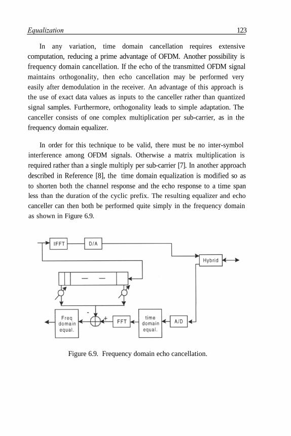
Equalization 123
In any variation, time domain cancellation requires extensivecomputation, reducing a prime advantage of OFDM. Another possibility isfrequency domain cancellation. If the echo of the transmitted OFDM signalmaintains orthogonality, then echo cancellation may be performed veryeasily after demodulation in the receiver. An advantage of this approach isthe use of exact data values as inputs to the canceller rather than quantizedsignal samples. Furthermore, orthogonality leads to simple adaptation. Thecanceller consists of one complex multiplication per sub-carrier, as in thefrequency domain equalizer.
In order for this technique to be valid, there must be no inter-symbolinterference among OFDM signals. Otherwise a matrix multiplication is
required rather than a single multiply per sub-carrier [7]. In another approachdescribed in Reference [8], the time domain equalization is modified so asto shorten both the channel response and the echo response to a time spanless than the duration of the cyclic prefix. The resulting equalizer and echo
canceller can then both be performed quite simply in the frequency domainas shown in Figure 6.9.
Figure 6.9. Frequency domain echo cancellation.
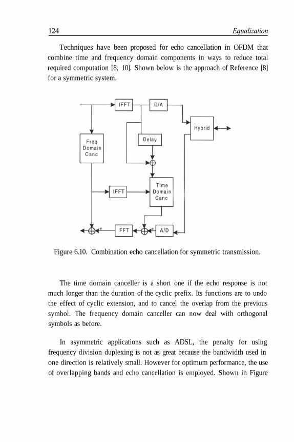
124 Equalization
Techniques have been proposed for echo cancellation in OFDM thatcombine time and frequency domain components in ways to reduce totalrequired computation [8, 10]. Shown below is the approach of Reference [8]for a symmetric system.
Figure 6.10. Combination echo cancellation for symmetric transmission.
The time domain canceller is a short one if the echo response is notmuch longer than the duration of the cyclic prefix. Its functions are to undothe effect of cyclic extension, and to cancel the overlap from the previoussymbol. The frequency domain canceller can now deal with orthogonalsymbols as before.
In asymmetric applications such as ADSL, the penalty for usingfrequency division duplexing is not as great because the bandwidth used inone direction is relatively small. However for optimum performance, the useof overlapping bands and echo cancellation is employed. Shown in Figure

Equalization 125
6.11 and Figure 6.12 are modifications of the previous structure [8] when the
same OFDM symbol rate but different numbers of sub-carriers are used ineach direction, with overlap of the frequencies of some of the sub-carriers.
Figure 6.11. Echo cancellation where the transmit rate is lower than receiverate.
Figure 6.11 illustrates a case in which the transmit rate is lower than thereceive rate, as in the remote terminal of ADSL. Because the transmitspectrum is smaller than the receive spectrum, it is replicated so that thenumber of sub-carriers is increased to equal that of the received signal. Forthe time domain portion of the echo canceller, the transmit signal isinterpolated to the higher rate by inserting the appropriate number of zeroesbetween the time samples.

126 Equalization
Figure 6.12. Echo cancellation where the receive rate is lower than transmitrate.
The converse case, in which the transmit rate is higher than the receiverate, as in the central office terminal of an ADSL link, is shown Figure 6.12.The size of the input to the frequency domain canceller is reduced by foldingsubsets of the OFDM symbol on top of each other and adding them toproduce a number of sub-carriers equal to the number received. The timedomain sampling rate is reduced by computing the short echo at furtherspaced points.
Initial adaptation, for any echo cancellation structure, may be performedat the same time and with the same training signals as the equalization at theother end. Having the remote transmitter silent improves this initialadaptation.
Equalization 127
6.6 Appendix — Joint InnovationRepresentation of ARMA Models
Some of the least squares estimation algorithms developed for AR
models such as ladder form realization, can be extended to ARMA models
by using embedding technique. Namely, an ARMA model can be embedded
into a two channel AR model of joint input/output process [11]. The same
approach can be used to model an equalizer for an ARMA channel by
extending the results of the equalizer design for AR channels. Unlike AR
models, the covariance matrix of an ARMA model is not Toeplitz and thatresults in some numerical computational difficulties. Therefore, by using
embedding techniques we can transform an ARMA model to a multi-channel
AR model with a block-Toeplitz covariance matrix.
First, we present a geometric interpretation of prediction techniques forARMA processes which is the basis for understanding Levinson Algorithm.
In linear prediction theory, we predict by a linear combination of
previous m samples as a m-th order linear predictor,
such that an error criteria like
is minimized. The concept of an innovation process is a critical one inprediction and estimation. It represents the amount of new information
obtained by observing a new sample which was not available in previous
observations:
Estimation of sample using the previous m samples leads to an mth
order forward linear predictor

128 Equalization
while using future m samples leads to a backward mth order linear predictor
Error terms for backward and forward predictors represent an innovationprocess.These error terms are defined as:
A recursive implementation of linear predictors utilizes Gram-Schmidt
orthogonalization to transform samples into orthogonal random variables
[12].
By interpretation of the expression in Equation 6.41 as a metric of the
Hilbert space spanned by process x, a useful geometrical representation forlinear prediction can be offered as shown in Figure 6.13.
Next we briefly review the Levinson algorithm which is the origin ofimportant concepts such as lattice filters and equalizers. Originally, theLevinson algorithm was proposed as an efficient numerical technique forinverting toeplitz matrices.

Equalization 129
Figure 6.13. Geometric interpretation of linear predictors.
Its order-recursive nature leads to important concepts in estimation andequalization. Minimizing the error criteria 6.41 for the predictor of order mresults in the normal equation
where is Toeplitz matrix of correlations with
The Levinson algorithm calculates the n coefficients of n-th order linearpredictor using n-1 coefficients of (n-1)th order linear predictor. As areference we provide the scalar Levinson equations:
Initialization:
Recursion:

130 Equalization
where represents i-th coefficient of he k-th order predictor. In the
above equations, we did not explicitly distinguish between backward and
forward coefficients because optimal backward coefficients are reversed in
time and complex conjugate of optimal forward predictor coefficients.
When the exact order of the predictor is unknown, we can monitor the
error term after each iteration. An extensive treatment of this issue is
discussed in model order estimation theory.
The above order recursive technique is the basis of lattice representationof prediction filter as shown in Figure 6.14.
Figure 6.14. Lattice filter representation of predictors.
In general, an ARMA model can be represented as:

Equalization 131
where is the input process and represents the output process. The
innovation process of which represents additional information obtained
from observation of sample is:
where
The problem of linear prediction is: given a set of observed samples ofan estimate of unobserved sample is
required, usually without covariance information. The prediction filter ischosen to minimize the power of prediction error which means designing a
filter of the form
such that
where is as close to a white noise process as possible.
One approach to linear prediction of ARMA models is to introduce aninnovation process for input then embed it into a two-channel AR
process. The general approach for embedding is discussed extensively in theliterature. Here we discuss the embedding technique for the special case

132 Equalization
where is white. By introducing the augmented process
the new prediction error is
where
and
Geometric interpretation of the ARMA model using the embeddedtechnique is straightforward and useful. In the ARMA model the space ofobservations is spanned by augmented process [x, y]. Then the joint
backward and forward innovations can be interpreted as orthogonalprojections on the sub-spaces spanned by future and past observationrespectively.
The Levinson recursion algorithm can be applied to the augmented(multi-channel) system as well. However, unlike the scalar case, backwardand forward predictor coefficients are not time-reversed and complexconjugate versions of each other.
References
1. Bingham, J.A.C. "Multicarrier Modulation for Data Transmission: an Idea whose Timehas Come." IEEE Commun. Mag.: May 1990; 28: 5-14.
2. Chow, J., Cioffi J., Bingham J. "Equalizer Training Algorithms for MulticarrierModulation Systems." IEEE Int. Conf. Commun; 1993: 761-765.

Equalization 133
3. Falconer, D., Magee F. "Adaptive Channel Memory Truncation for MaximumLikelihood Sequence Estimation." Bell System Tech. Journal; Nov 1973; 52: 1541-1562.
4. Lee, E.A., Messerschmitt D.G. Digital Communication. Boston: Kluwer AcademicPublisher, 1994.
5. Al-Dhahir, N., Cioffi J. "Optimum Finite Length Equalization for MulticarrierTransceiver." IEEE Globecom; 1994: 1884-1888.
6. Cioffi, J.M., Bingham J.A.C. "A Data Driven Multitone Echo Canceller." IEEE Trans.Commun.; Oct 1994; 42; 10: 2853-2867.
7. Yang, J., Roy S., Lewis N.H. "Data-Driven Echo Cancellation for a MultitoneModulation System." IEEE Trans. Commun.; May 1996;44; 5: 2134-2144.
8. Melsa, P.J.W., Younce R.C., Rohrs C.E. "Impulse Response Shortening for DiscreteMultitone Transceivers." IEEE Trans. Commun.; Dec 1996; 44; 12: 1662-1672.
9. Ho, M., Cioffi J.M., Bingham J.A.C. "High-Speed Full-Duplex Echo Cancellation forMultitone Modulation." IEEE Int. Conf. Commun.; 1993: 772-76.
10. Ho, M., Cioffi J.M., Bingham J.A.C. "Discrete Multitone Echo Cancellation." IEEETrans. Commun.; Jul 1996; 44; 7: 817-825.
11. Lee, D. L., Friedlander B., Morf M. "Recursive Ladder Algorithms for ARMAModeling." IEEE Trans. Automatic Control, Aug 1982; AC-27: 4.
12. Kay, S.M. Modern Spectral Estimation. Upper Saddle River, NJ: Prentice Hall, 1988.
Chapter 7 Channel Coding
7.1 Need for Coding
In almost all applications of multi-carrier modulation, satisfactoryperformance cannot be achieved without the addition of some form ofcoding. In wireless systems subjected to fading, extremely high signal-to-noise ratios are required to achieve reasonable error probability. In addition,interference from other wireless channels is frequently severe. On wirelinesystems, large constellation sizes are commonly employed to achieve highbit rates. Coding in this case is essential for achieving the highest possiblerates in the presence of crosstalk and impulsive and other interference.
Proper coding design is extremely important for a digital communicationlink [1]. A designer should take several design factors into account. Thoseinclude required coding gain for intended link budget, channelcharacteristics, source coding requirements, modulation, etc. Coding inOFDM systems has an additional dimension. It can be implemented in timeand frequency domain such that both dimensions are utilised to achievebetter immunity against frequency and time selective fading. Obviously,
135

136 Channel Coding
interleaving plays an important role to achieve the above goal as shown inFigure 7.1. A combination of block coding and convolutional coding alongwith proper time/frequency interleaving constitutes a concatenated codingstrategy. A new generation of parallel concatenated coding, namely turbocoding, also seems promising for some OFDM applications.
In this chapter, performance of block, convolutional, and trellis coding,and issues concerning concatenated and turbo coding are discussed. Acomparison of their performance with theoretical bounds is also presented.
Figure 7.1. Two-dimensional coding for OFDM.
7.2 Block Coding in OFDM
In classical block coding, input data are blocked into groups of k bits,and each block is mapped into an output block of n bits, where n > k. In the
canonical form, n - k parity checks are computed among the input bits
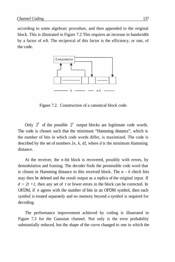
Channel Coding 137
according to some algebraic procedure, and then appended to the originalblock. This is illustrated in Figure 7.2 This requires an increase in bandwidthby a factor of n/k. The reciprocal of this factor is the efficiency, or rate, ofthe code.
Figure 7.2. Construction of a canonical block code.
Only 2k of the possible 2n output blocks are legitimate code words.The code is chosen such that the minimum “Hamming distance”, which isthe number of bits in which code words differ, is maximized. The code isdescribed by the set of numbers [n, k, d], where d is the minimum Hammingdistance.
At the receiver, the n–bit block is recovered, possibly with errors, bydemodulation and framing. The decoder finds the permissible code word thatis closest in Hamming distance to this received block. The n – k check bitsmay then be deleted and the result output as a replica of the original input. Ifd = 2t +1, then any set of t or fewer errors in the block can be corrected. InOFDM, if n agrees with the number of bits in an OFDM symbol, then eachsymbol is treated separately and no memory beyond a symbol is required fordecoding.
The performance improvement achieved by coding is illustrated inFigure 7.3 for the Gaussian channel. Not only is the error probabilitysubstantially reduced, but the shape of the curve changed to one in which the
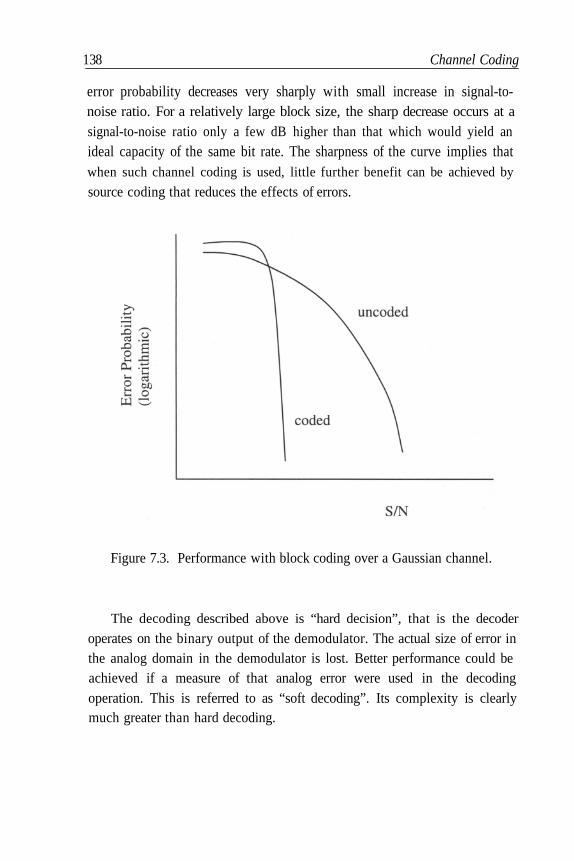
138 Channel Coding
error probability decreases very sharply with small increase in signal-to-noise ratio. For a relatively large block size, the sharp decrease occurs at asignal-to-noise ratio only a few dB higher than that which would yield anideal capacity of the same bit rate. The sharpness of the curve implies thatwhen such channel coding is used, little further benefit can be achieved by
source coding that reduces the effects of errors.
Figure 7.3. Performance with block coding over a Gaussian channel.
The decoding described above is “hard decision”, that is the decoder
operates on the binary output of the demodulator. The actual size of error inthe analog domain in the demodulator is lost. Better performance could beachieved if a measure of that analog error were used in the decodingoperation. This is referred to as “soft decoding”. Its complexity is clearlymuch greater than hard decoding.
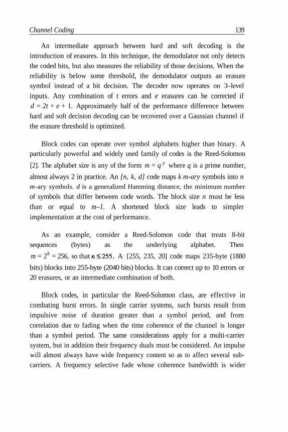
Channel Coding 139
An intermediate approach between hard and soft decoding is theintroduction of erasures. In this technique, the demodulator not only detectsthe coded bits, but also measures the reliability of those decisions. When thereliability is below some threshold, the demodulator outputs an erasuresymbol instead of a bit decision. The decoder now operates on 3–level
inputs. Any combination of t errors and e erasures can be corrected ifd = 2t + e + 1. Approximately half of the performance difference betweenhard and soft decision decoding can be recovered over a Gaussian channel if
the erasure threshold is optimized.
Block codes can operate over symbol alphabets higher than binary. Aparticularly powerful and widely used family of codes is the Reed-Solomon
[2]. The alphabet size is any of the form m = q p where q is a prime number,
almost always 2 in practice. An [n, k, d] code maps k m-ary symbols into nm-ary symbols. d is a generalized Hamming distance, the minimum number
of symbols that differ between code words. The block size n must be less
than or equal to m–1. A shortened block size leads to simplerimplementation at the cost of performance.
As an example, consider a Reed-Solomon code that treats 8-bitsequences (bytes) as the underlying alphabet. Then
m = 28 = 256, so that A {255, 235, 20] code maps 235-byte (1880
bits) blocks into 255-byte (2040 bits) blocks. It can correct up to 10 errors or20 erasures, or an intermediate combination of both.
Block codes, in particular the Reed-Solomon class, are effective incombating burst errors. In single carrier systems, such bursts result fromimpulsive noise of duration greater than a symbol period, and from
correlation due to fading when the time coherence of the channel is longerthan a symbol period. The same considerations apply for a multi-carriersystem, but in addition their frequency duals must be considered. An impulsewill almost always have wide frequency content so as to affect several sub-carriers. A frequency selective fade whose coherence bandwidth is wider
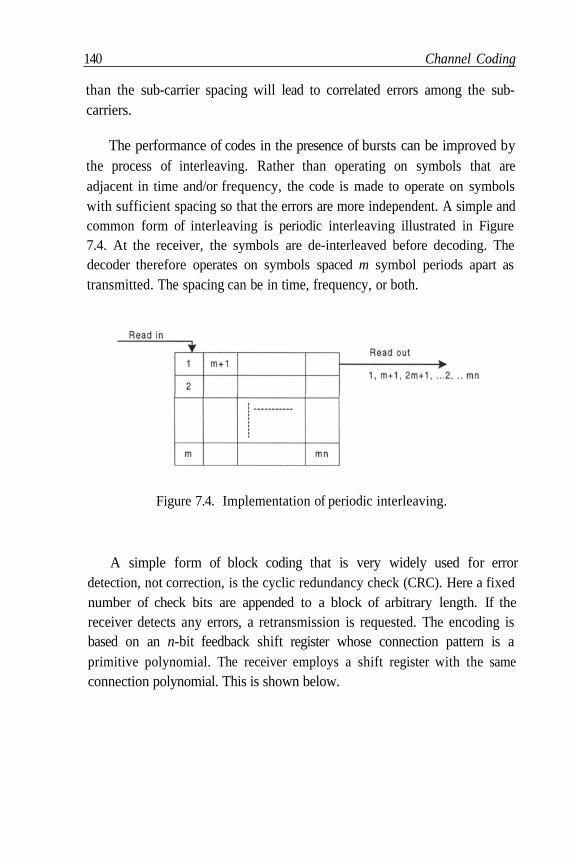
140 Channel Coding
than the sub-carrier spacing will lead to correlated errors among the sub-carriers.
The performance of codes in the presence of bursts can be improved bythe process of interleaving. Rather than operating on symbols that areadjacent in time and/or frequency, the code is made to operate on symbolswith sufficient spacing so that the errors are more independent. A simple andcommon form of interleaving is periodic interleaving illustrated in Figure7.4. At the receiver, the symbols are de-interleaved before decoding. Thedecoder therefore operates on symbols spaced m symbol periods apart astransmitted. The spacing can be in time, frequency, or both.
Figure 7.4. Implementation of periodic interleaving.
A simple form of block coding that is very widely used for errordetection, not correction, is the cyclic redundancy check (CRC). Here a fixednumber of check bits are appended to a block of arbitrary length. If thereceiver detects any errors, a retransmission is requested. The encoding isbased on an n-bit feedback shift register whose connection pattern is aprimitive polynomial. The receiver employs a shift register with the sameconnection polynomial. This is shown below.
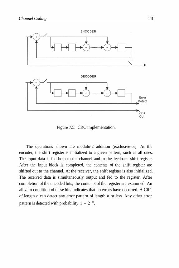
Channel Coding 141
Figure 7.5. CRC implementation.
The operations shown are modulo-2 addition (exclusive-or). At theencoder, the shift register is initialized to a given pattern, such as all ones.The input data is fed both to the channel and to the feedback shift register.After the input block is completed, the contents of the shift register areshifted out to the channel. At the receiver, the shift register is also initialized.The received data is simultaneously output and fed to the register. Aftercompletion of the uncoded bits, the contents of the register are examined. Anall-zero condition of these bits indicates that no errors have occurred. A CRCof length n can detect any error pattern of length n or less. Any other error
pattern is detected with probability 1 – 2 – n .
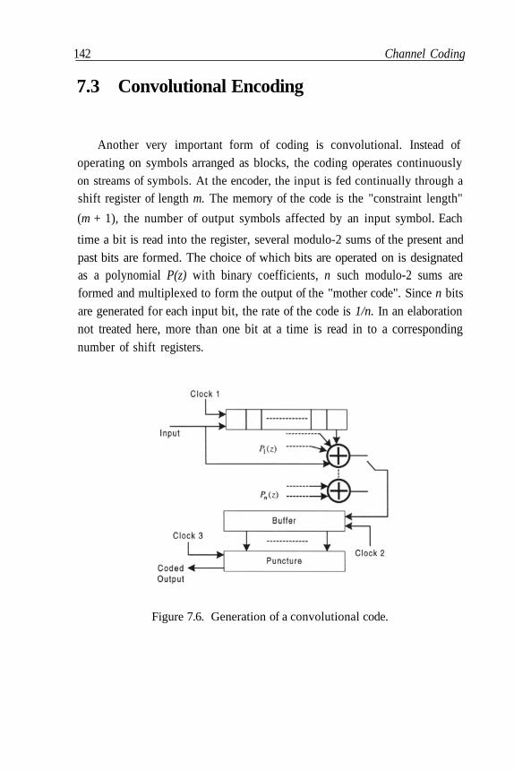
142 Channel Coding
7.3 Convolutional Encoding
Another very important form of coding is convolutional. Instead ofoperating on symbols arranged as blocks, the coding operates continuouslyon streams of symbols. At the encoder, the input is fed continually through a
shift register of length m. The memory of the code is the "constraint length"
(m + 1), the number of output symbols affected by an input symbol. Each
time a bit is read into the register, several modulo-2 sums of the present andpast bits are formed. The choice of which bits are operated on is designatedas a polynomial P(z) with binary coefficients, n such modulo-2 sums areformed and multiplexed to form the output of the "mother code". Since n bitsare generated for each input bit, the rate of the code is 1/n. In an elaborationnot treated here, more than one bit at a time is read in to a correspondingnumber of shift registers.
Figure 7.6. Generation of a convolutional code.

Channel Coding 143
The rate of the code can be increased by the process of puncturing. Thisinvolves deleting some of the bits generated by the mother code. The process
of generating a convolutional code is shown in Figure 7.6. In addition,interleaving may be applied to a convolutional code in a manner similar to ablock code.
A convolutional code can be described by a state diagram. For a binary
convolutional code, the number of states is s = 2m , where m is the number of
shift register stages in the transmitter. In the state diagram shown in Figure7.7, the transitions from a current state to a next state are determined by thecurrent input bit, and each transition produces an output of n bits.
Figure 7.7. State diagram of a convolutional code.
A particular advantage of convolutional codes is the relative ease ofdecoding. Sequence estimation techniques are applicable, in particular theViterbi algorithm. The Viterbi algorithm has the desirable properties of notonly very efficient computation, but also a fixed amount of computation persymbol and an orderly flow of computation. The low complexity ofdecoding permits soft decision decoding, where the minimum Euclideandistance between the received sequence and all allowed sequences, ratherthan Hamming distance, is used to form decisions.
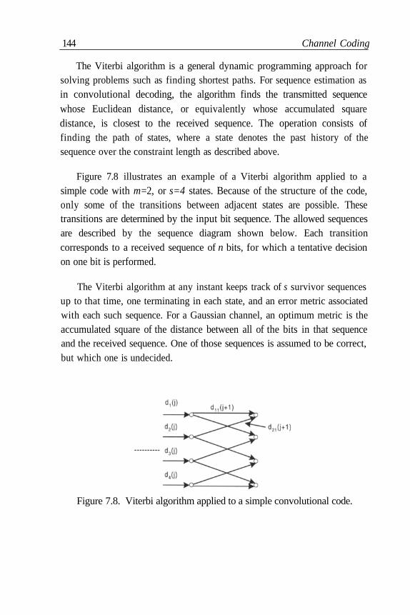
144 Channel Coding
The Viterbi algorithm is a general dynamic programming approach forsolving problems such as finding shortest paths. For sequence estimation asin convolutional decoding, the algorithm finds the transmitted sequencewhose Euclidean distance, or equivalently whose accumulated squaredistance, is closest to the received sequence. The operation consists offinding the path of states, where a state denotes the past history of thesequence over the constraint length as described above.
Figure 7.8 illustrates an example of a Viterbi algorithm applied to asimple code with m=2, or s=4 states. Because of the structure of the code,only some of the transitions between adjacent states are possible. Thesetransitions are determined by the input bit sequence. The allowed sequencesare described by the sequence diagram shown below. Each transitioncorresponds to a received sequence of n bits, for which a tentative decisionon one bit is performed.
The Viterbi algorithm at any instant keeps track of s survivor sequencesup to that time, one terminating in each state, and an error metric associatedwith each such sequence. For a Gaussian channel, an optimum metric is theaccumulated square of the distance between all of the bits in that sequenceand the received sequence. One of those sequences is assumed to be correct,but which one is undecided.
Figure 7.8. Viterbi algorithm applied to a simple convolutional code.

Channel Coding 145
When a group of n bits corresponding to one information bit is received,each survivor sequence is extended according to the added metricsassociated with the new input. Each possible sequence terminating in eachnew state is evaluated, and all sequences other than the one with minimummetric is discarded.
The figure shows how the survivor sequence for state 1 is chosen. Thesame process is performed for each state. For r(k) the received signal overtime k and t(k) the transmitted symbols, then
where is the symbol sequence associated with the transition from
state p to state q. The values of r and t may be complex. The survivorsequence chosen for state 1 at time j+1 is the one whose accumulated metricis
Only allowed paths pq are examined. Then at time j+1 we again haveone survivor sequence terminating in each state, each one being an extension
of a previous survivor sequence. It is necessary to make a decision at eachstep. In almost all cases, if we project far enough into the past, all survivorsequences will have a common beginning. In practice going back N =6(m+1) is sufficient. So at any time the stored survivor sequences are Ninformation symbols long, one past information symbol is read out, and thedelay through the decoder is N.
The squared error is optimum for a Gaussian channel, but a sub-optimum metric for a fading channel. Nevertheless it is frequently usedbecause of its simplicity. For optimum performance over a fading channel,
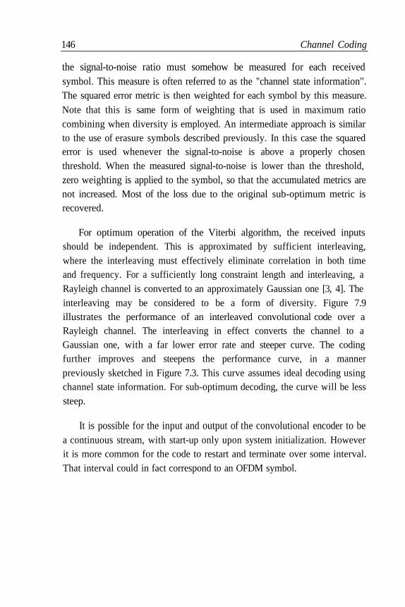
146 Channel Coding
the signal-to-noise ratio must somehow be measured for each receivedsymbol. This measure is often referred to as the "channel state information".The squared error metric is then weighted for each symbol by this measure.
Note that this is same form of weighting that is used in maximum ratiocombining when diversity is employed. An intermediate approach is similarto the use of erasure symbols described previously. In this case the squarederror is used whenever the signal-to-noise is above a properly chosenthreshold. When the measured signal-to-noise is lower than the threshold,zero weighting is applied to the symbol, so that the accumulated metrics arenot increased. Most of the loss due to the original sub-optimum metric isrecovered.
For optimum operation of the Viterbi algorithm, the received inputsshould be independent. This is approximated by sufficient interleaving,where the interleaving must effectively eliminate correlation in both timeand frequency. For a sufficiently long constraint length and interleaving, aRayleigh channel is converted to an approximately Gaussian one [3, 4]. Theinterleaving may be considered to be a form of diversity. Figure 7.9illustrates the performance of an interleaved convolutional code over aRayleigh channel. The interleaving in effect converts the channel to aGaussian one, with a far lower error rate and steeper curve. The codingfurther improves and steepens the performance curve, in a mannerpreviously sketched in Figure 7.3. This curve assumes ideal decoding usingchannel state information. For sub-optimum decoding, the curve will be lesssteep.
It is possible for the input and output of the convolutional encoder to bea continuous stream, with start-up only upon system initialization. Howeverit is more common for the code to restart and terminate over some interval.That interval could in fact correspond to an OFDM symbol.

Channel Coding 147
Figure 7.9. Performance of a convolutional code over a Rayleigh fadingchannel.
In this case the encoder and decoder start in a given state and are forced
to terminate in a given state. This allows the Viterbi decoder to eliminate allsurvivor states but one at the end and to read out the remainder of the storeddetected sequence.
7.4 Concatenated Coding
Combining convolutional and block codes in a concatenated code is aparticularly powerful technique. The block code is the outer code, that is it isapplied first at the transmitter and last at the receiver. The innerconvolutional code is very effective at reducing the error probability,
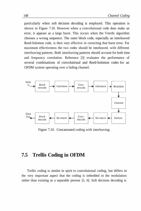
148 Channel Coding
particularly when soft decision decoding is employed. This operation isshown in Figure 7.10. However when a convolutional code does make anerror, it appears as a large burst. This occurs when the Viterbi algorithmchooses a wrong sequence. The outer block code, especially an interleavedReed-Solomon code, is then very effective in correcting that burst error. Formaximum effectiveness the two codes should be interleaved, with differentinterleaving patterns. Both interleaving patterns should account for both time
and frequency correlation. Reference [3] evaluates the performance ofseveral combinations of convolutional and Reed-Solomon codes for anOFDM system operating over a fading channel.
Figure 7.10. Concatenated coding with interleaving.
7.5 Trellis Coding in OFDM
Trellis coding is similar in spirit to convolutional coding, but differs inthe very important aspect that the coding is imbedded in the modulation
rather than existing as a separable process [5, 6]. Soft decision decoding is
Channel Coding 149
based on minimum Euclidean distance of sequences, and is part of thedemodulation procedure.
This is in keeping with the basic philosophy of information theory. InShannon's original paper, capacity is achieved by assigning a differentwaveform for each complete message, and the length of the message isallowed to approach infinity. Nowhere is the message described as asequence of bits or symbols. The receiver chooses the message as the oneclosest to the received waveform. Trellis coding is a practical approximationto this theoretical scheme.
Rather than adding redundant bits or symbols prior to modulation,redundancy is introduced by using constellations with more points thanwould be required without coding. Usually the number of points is doubled.The number of symbols per second is unchanged, therefore the bandwidthrequired is also unchanged. Since there are more possible points per symbol,it may appear that the error probability for a given signal-to-noise ratiowould increase. However, as in convolutional coding, dependencies areintroduced among the different symbols in that only certain sequences ofconstellation points are allowed. By properly making use of these constraintsin the receiver, as in convolutional decoding, the error probability actuallydecreases. A measure of performance improvement is the "coding gain",which is the difference in S/N between a coded and an uncoded system ofthe same information rate that produces a given error probability.
The first step in designing a trellis code is to form an expandedconstellation and to partition it into subsets. The points within each subsetare made far apart in Euclidean distance, and will correspond to uncodedbits. The remaining, or coded bits, determine the choice of subset. Onlycertain sequences of subsets are permitted, those sequences beingdetermined by a simple convolutional code. As in convolutional coding, thesequence is best described by a state transition diagram or " trellis". In orderto keep allowed sequences far apart, the constellation subsets are chosen so

150 Channel Coding
that those corresponding to branching in and out of each state havemaximum distance separation.
We will illustrate the procedure with a simple trellis code that uses a 16-point QAM constellation to carry 3 bits per symbol. The technique is alsoapplicable to phase modulation, where the number of phases is increased.Shown in Figure 7.11 is a partition of the constellation into 4 subsets of 4points each, where the labelling of points denotes subset membership.
Figure 7.11. An expanded constellation partitioned for Trellis coding.
Figure 7.12. Implementation of a Trellis code.

Channel Coding 151
Figure 7.12 shows the mapping of 3-bit input symbols into constellationpoints. Two of the input bits, and , are uncoded and determine which
member of a subset is used. The third bit is fed to a rate-1/2 convolutional
encoder whose 2-bit output determines which subset is used.
Figure 7.13 is the state diagram of the code. The states are labelledaccording to the contents of the shift register in the convolutional encoder.The labels of the transitions indicate which subset is used when thattransition occurs.
Figure 7.13. State diagram of the Trellis code.
At the receiver, a Viterbi algorithm is used for the combineddemodulation and decoding. For each received symbol the distance to thenearest member of each subset is measured, as shown in Figure 7.14. Thesquare of this value serves as the metric in extending the survivor states ofthe Viterbi algorithm. For each survivor state, not only must the coded bitsand accumulated squared distance be stored, but also the uncoded bitscorresponding to which member of the subset was the nearest point for eachsymbol.
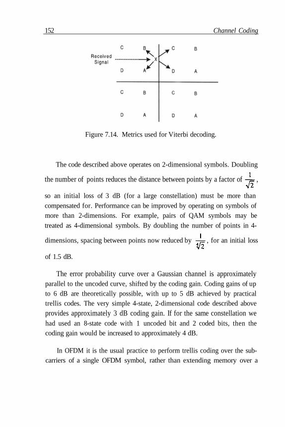
152 Channel Coding
Figure 7.14. Metrics used for Viterbi decoding.
The code described above operates on 2-dimensional symbols. Doubling
the number of points reduces the distance between points by a factor of ,
so an initial loss of 3 dB (for a large constellation) must be more thancompensated for. Performance can be improved by operating on symbols ofmore than 2-dimensions. For example, pairs of QAM symbols may betreated as 4-dimensional symbols. By doubling the number of points in 4-
dimensions, spacing between points now reduced by , for an initial loss
of 1.5 dB.
The error probability curve over a Gaussian channel is approximatelyparallel to the uncoded curve, shifted by the coding gain. Coding gains of upto 6 dB are theoretically possible, with up to 5 dB achieved by practicaltrellis codes. The very simple 4-state, 2-dimensional code described aboveprovides approximately 3 dB coding gain. If for the same constellation wehad used an 8-state code with 1 uncoded bit and 2 coded bits, then thecoding gain would be increased to approximately 4 dB.
In OFDM it is the usual practice to perform trellis coding over the sub-carriers of a single OFDM symbol, rather than extending memory over a
Channel Coding 153
greater interval of time. At the beginning of each OFDM symbol, the code is
started in a known state. The code is forced to a known state at the end of anOFDM symbol. Any null sub-carriers are skipped. Variable sizeconstellations are readily handled by using a fixed number of coded bits oneach sub-carrier and a variable number of uncoded bits.
7.6 Turbo Coding in OFDM
Turbo coding has recently been used in many communication systemssuccessfully. Random-like structure of turbo codes has resulted inoutstanding performance by providing small error rates at information ratesof close to theoretical channel capacity. In this section, we briefly review
some fundamental features of turbo coding and explain why it is a goodpotential candidate for OFDM systems.
In general a turbo code comprises two or more concatenated or parallelcodes. A typical turbo code includes parallel concatenated convolutionalcodes where the information bits are coded by two or more recursive
systematic convolutional codes each applied to permutations of theinformation sequence as in Figure 7.15. However, the same iterative turbodecoding principle can be applied to serially and hybrid concatenated codes[7]. The high error correction power of turbo coders originates from randomlike coding achieved by random interleaving in conjunction withconcatenated coding and iterative decoding using (almost) uncorrelatedextrinsic information.
The structure and complexity of turbo encoder design is restricted byother system parameters. Here, we briefly review some of the critical issueswhich directly impact the code structure. Decoding Delay is critical forreceiver design. Since the decoding structure of turbo codes is iterative and
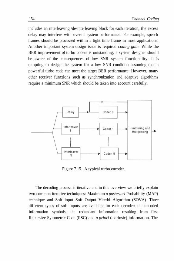
154 Channel Coding
includes an interleaving /de-interleaving block for each iteration, the excessdelay may interfere with overall system performance. For example, speechframes should be processed within a tight time frame in most applications.Another important system design issue is required coding gain. While theBER improvement of turbo coders is outstanding, a system designer should
be aware of the consequences of low SNR system functionality. It istempting to design the system for a low SNR condition assuming that a
powerful turbo code can meet the target BER performance. However, many
other receiver functions such as synchronization and adaptive algorithmsrequire a minimum SNR which should be taken into account carefully.
Figure 7.15. A typical turbo encoder.
The decoding process is iterative and in this overview we briefly explaintwo common iterative techniques: Maximum a posteriori Probability (MAP)technique and Soft input Soft Output Viterbi Algorithm (SOVA). Threedifferent types of soft inputs are available for each decoder: the uncodedinformation symbols, the redundant information resulting from firstRecursive Symmetric Code (RSC) and a priori (extrinsic) information. The
Channel Coding 155
output is a weighted version of uncoded information, a priori informationand new extrinsic information.
In general, a symbol-by-symbol MAP algorithm is optimal for stateestimation of a Markov process. MAP algorithms for turbo decodingcalculate the logarithm of the ratio of a posteriori probability (APP) of each
information bit being one to the a posteriori probability of the bit being zero.
The MAP technique is complicated and requires non-linear operations whichmakes it less attractive for practical purposes. In comparison, a
simplification of MAP algorithm, namely, Soft Output Viterbi Algorithm(SOVA) leads to a practical sub-optimum technique. While performance isslightly inferior to an optimal MAP algorithm, the complexity issignificantly less. MAP takes into account all paths by splitting them intotwo sets, namely, the path that has an information bit one at a particular stepand paths which have bit zero at that step and returns the log likelihood ratioof the two. SOVA considers only the survivor path of the Viterbi algorithm.
Therefore, only the survived competing path which joins the path chosen in
the Viterbi algorithm is taken into account for reliability estimation.
While the encoders have a parallel structure, the decoders operate inserial which results in an asymmetric overall structure. For example, in thefirst iteration the first decoder has no a priori information [9].
As discussed before, coding schemes for OFDM systems takeadvantages of coding in both time and frequency in conjunction with properinterleaving. This provides extra protection against time and frequencyselective fading. Use of turbo coding for OFDM systems is seriously beingconsidered for several wireless standards. The depth of interleaving can berestricted to one OFDM block which provides correlation between symbolsmodulated by different sub-carriers and subjected to independent selectivefading.

156 Channel Coding
Figure 7.16. A turbo decoder structure.
Another coding scheme supports inter-block interleaving which can beintelligently designed to provide time and frequency correlation. While theformer technique does not impose extra delay at the receiver, the lattertechnique gives another degree of freedom to the system designer. Thechoice of proper coding scheme depends on system requirements andapplications.
References
1. Costello, D.J., Costello Lin. Error Control Coding. Englewood Cliffs, NJ: Prentice-Hall, 1983.
2. Wicker, B., Bhargava V.K. Reed-Solomon Codes and Their Applications. New York:IEEE Press, 1994.
3. Alard M., Lassalle R. "Principles of Modulation and Channel Coding for DigitalBroadcasting for Mobile Receivers." EBU Review; Aug 1987; 224: 47-69.

Channel Coding 157
4. Pommier D., Wu Y. "Interleaving or Spectrum Spreading in Digital Radio Intended forVehicles." EBU Review; Jun 1986; 217: 31-44.
5. Ungerboeck, G. "Trellis Coded Modulation with Redundant Signal Sets." IEEECommun. Mag.; Feb 1987; 25; 2: 5-21.
6. Biglieri, D., Divsalar D., McLane P.J., Simon M.K. Introduction to Trellis-CodedModulation with Applications. New York: Macmillan, 1991.
7. Hagenauer, J., Offer E., Papke L. "Iterative Decoding of Binary Block and ConvolutionalCodes." IEEE Trans. Information Theory ;Feb 1987; 25; 2: 5-21.
8. Jung, P. "Comparison of Turbo-Code Decoders Applied to Short Frame TransmissionSystems." IEEE Journal on Selected Areas in Communications; Apr 1996; 14; 3.
9. Hoeher, P. "New Iterative Turbo Decoding Algorithms" Proceeding of The InternationalSymposium on Turbo Codes; Brest, France; 1997.

Chapter 8 ADSL
8.1 Wired Access to High Rate Digital Services
A ubiquitous communication channel is the subscriber line, or loop,consisting of an unshielded twisted pair of wires, connecting any home oroffice to a telephone company’s central office. The overwhelming majorityof these channels are used to carry analog voice conversations, which requirea bandwidth of less than 4 kHz. It has long been recognized that mostsubscriber lines can support a much wider bandwidth, in particular, to carryhigh rate digital signals. The first such widespread use is for access to basicrate ISDN, in which the subscriber line carries 160 kb/s simultaneously inboth directions over a single pair.
More recently, higher rates have been introduced into numeroussystems. Of particular interest here is ADSL which is primarily intended toprovide access for residential applications [1, 2]. Most of such applicationsrequire a high data rate in the downstream direction (to the customer) and amuch lower rate upstream (from the customer). The primary applications ofADSL are the delivery of digitally encoded video, and access to digital
159
160 ADSL
services, particularly the Internet. ADSL meets these needs by providing ahigh rate digital downstream signal of over 1 Mb/s, a moderate rate upstreamsignal, and a normal analog voice channel, all over a single wire-pair.Because virtually all customers have a wire-pair channel providing voiceservice, no additional channel need be installed to provide this new service.It only requires the installation of terminating equipment at the customers’premises and at the central offices. OFDM, typically referred to as DMT(Discrete Multi-Tone) in this application, has been adopted as the standardfor transmission of the digital information. Several varieties of ADSL exist,
differing primarily in the bit rates carried and the set of subscriber lines overwhich satisfactory performance is achieved.
8.2 Properties of the Wire-Pair Channel
Before discussing the transmission techniques, it is essential to firstdescribe the channel — both its transmission properties and the types ofinterference to which it is subject. As with any communication channel, acombination of both factors must be considered in determining theperformance that can be achieved.
The connection between the subscriber and the central office consists ofseveral sections, each consisting of a wire-pair bundled in a cable with many
other wire-pairs [3, 4, 5]. Insulation on modern cables is polyethylene,although older paper pulp cable is still present in much of the plant. Thesections nearest the central office are referred to as feeder, where the cablesize is large but the wire gauge may be fine. Closer to the customer, thedistribution plant consists of smaller cables, but typically heavier gaugewire. Finally, the individual drop wire provides the final connection to the
subscriber. Wiring on premises may also be significant. Typical wire gaugesize throughout is 24-gauge (0.5 mm) or 26-gauge (0.4 mm). The overall

ADSL 161
length of the circuit can be up to 5.5 km. If it is greater than this distance,loading coils are usually added which improve transmission in the voicebandbut greatly restrict the bandwidth above 4 kHz. Loaded circuits therefore
cannot be used to provide any high rate digital service. Fortunately suchcircuits are rare and exist only in rural areas.
A trend is now taking place to introduce carrier systems and remoteswitches into subscriber plants. Such electronic equipment is connected tothe central office digitally, often using optical fiber. ADSL in this case needonly provide access from the subscriber to the remote electronic devicerather than all the way to the central office. A plan, referred to as the CarrierServing Area (CSA), envisions almost all future subscribers within 3.7 km ofeither a central office or of remote equipment if the cable used for the wholepath is 0.5 mm or larger, or 2.7 km if 0.4 mm wire is used. An additionalbenefit of this plan is the elimination of loaded circuits.
The transmission properties of a wire-pair are determined by its primaryconstants, the resistance R, inductance L, capacitance C, and conductance G
per unit length. At low frequencies, R is constant, but increases proportional
to at high frequencies (above about 200 kHz), due to skin effect. C is
very constant with frequency, and L declines slightly with frequency. The
conductance increases with frequency, but is small enough for moderncables that it may be neglected over the entire frequency range. Ignoringmismatched impedance effects, the transfer function of a line of length d is
where the complex propagation constant is given by
is the loss in nepers per unit length, and the phase shift in radians per
unit length. The phase distortion can, in general, be equalized, at least inprinciple. So, the loss has the primary effect on performance. However, itshould be noted that the phase distortion, that is the deviation from linear
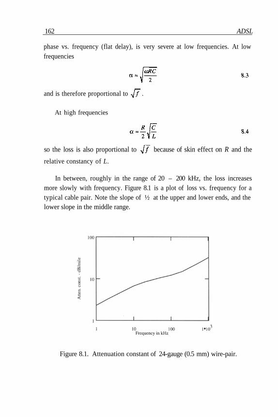
162 ADSL
phase vs. frequency (flat delay), is very severe at low frequencies. At lowfrequencies
and is therefore proportional to
At high frequencies
so the loss is also proportional to because of skin effect on R and the
relative constancy of L.
In between, roughly in the range of 20 – 200 kHz, the loss increasesmore slowly with frequency. Figure 8.1 is a plot of loss vs. frequency for atypical cable pair. Note the slope of ½ at the upper and lower ends, and thelower slope in the middle range.
Figure 8.1. Attenuation constant of 24-gauge (0.5 mm) wire-pair.
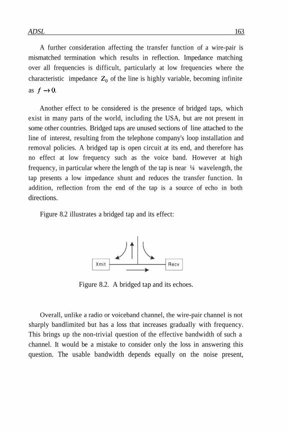
ADSL 163
A further consideration affecting the transfer function of a wire-pair ismismatched termination which results in reflection. Impedance matchingover all frequencies is difficult, particularly at low frequencies where the
characteristic impedance of the line is highly variable, becoming infinite
as
Another effect to be considered is the presence of bridged taps, whichexist in many parts of the world, including the USA, but are not present insome other countries. Bridged taps are unused sections of line attached to theline of interest, resulting from the telephone company's loop installation andremoval policies. A bridged tap is open circuit at its end, and therefore hasno effect at low frequency such as the voice band. However at high
frequency, in particular where the length of the tap is near ¼ wavelength, thetap presents a low impedance shunt and reduces the transfer function. Inaddition, reflection from the end of the tap is a source of echo in both
directions.
Figure 8.2 illustrates a bridged tap and its effect:
Figure 8.2. A bridged tap and its echoes.
Overall, unlike a radio or voiceband channel, the wire-pair channel is not
sharply bandlimited but has a loss that increases gradually with frequency.This brings up the non-trivial question of the effective bandwidth of such achannel. It would be a mistake to consider only the loss in answering thisquestion. The usable bandwidth depends equally on the noise present,
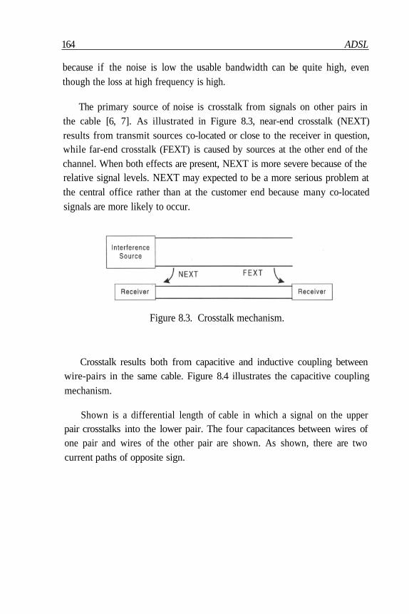
164 ADSL
because if the noise is low the usable bandwidth can be quite high, eventhough the loss at high frequency is high.
The primary source of noise is crosstalk from signals on other pairs inthe cable [6, 7]. As illustrated in Figure 8.3, near-end crosstalk (NEXT)results from transmit sources co-located or close to the receiver in question,while far-end crosstalk (FEXT) is caused by sources at the other end of thechannel. When both effects are present, NEXT is more severe because of therelative signal levels. NEXT may expected to be a more serious problem atthe central office rather than at the customer end because many co-located
signals are more likely to occur.
Figure 8.3. Crosstalk mechanism.
Crosstalk results both from capacitive and inductive coupling betweenwire-pairs in the same cable. Figure 8.4 illustrates the capacitive coupling
mechanism.
Shown is a differential length of cable in which a signal on the upperpair crosstalks into the lower pair. The four capacitances between wires ofone pair and wires of the other pair are shown. As shown, there are twocurrent paths of opposite sign.
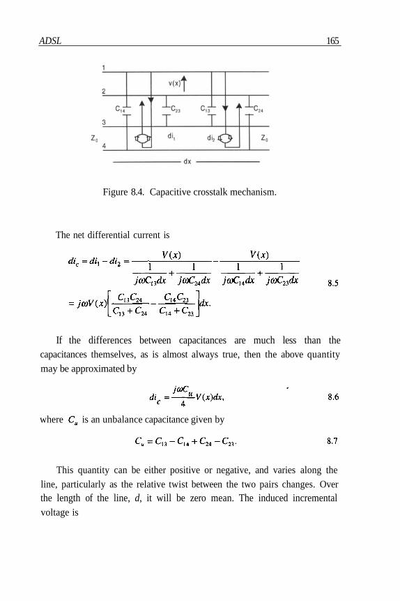
ADSL 165
Figure 8.4. Capacitive crosstalk mechanism.
The net differential current is
If the differences between capacitances are much less than thecapacitances themselves, as is almost always true, then the above quantity
may be approximated by
where is an unbalance capacitance given by
This quantity can be either positive or negative, and varies along the
line, particularly as the relative twist between the two pairs changes. Overthe length of the line, d, it will be zero mean. The induced incrementalvoltage is

166 ADSL
where it is assumed that the line is terminated in its characteristic impedancein both directions.
The inductive coupling may be treated similarly, as shown in Figure 8.5.
Figure 8.5. Inductive crosstalk mechanism.
Over the differential length, the mutual inductance is M dx. Then thedifferential induced voltage is
The near-end and far-end currents are
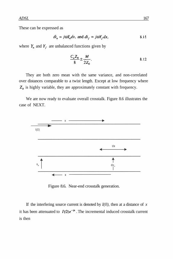
ADSL 167
These can be expressed as
where and are unbalanced functions given by
They are both zero mean with the same variance, and non-correlatedover distances comparable to a twist length. Except at low frequency where
is highly variable, they are approximately constant with frequency.
We are now ready to evaluate overall crosstalk. Figure 8.6 illustrates the
case of NEXT.
Figure 8.6. Near-end crosstalk generation.
If the interfering source current is denoted by I(0), then at a distance of x
it has been attenuated to The incremental induced crosstalk current
is then

168 ADSL
and similarly, the incremental crosstalk voltage is
When propagated back to the input, the contribution of this crosstalkcomponent is
and the total NEXT voltage is
This quantity is zero mean, with variance
Because is non-correlated over short distances, we can approximate
so that
For any but the shortest lines, We will further approximate
Then, lumping together the various constants,
We now have the important result that the NEXT power transferfunction,

ADSL 169
is proportional to and is independent of the line length except for very
short lines. The level of the transfer function is determined by the constant
It can also be specified by giving its value at some frequency Then
at any other frequency,
We can analyze the far-end crosstalk in a similar manner to obtain
The exponential factor arises from the fact that all crosstalk componentstravel a total distance of d, partly on the interfering pair, and the remainderon the interfered pair. When both NEXT and FEXT occur, the formerdominates at all frequencies of interest.
It is usual to model various system imperfections, such as finiteprecision digital implementations, as an added white Gaussian noise, with
spectral density This is usually a reasonably accurate model. In
addition, it eliminates singularities in signal-to-noise ratios in the presence ofonly crosstalk. It should be noted that at the relatively high receiver powerlevels in wire-pair systems, actual thermal noise is so far below the signalthat it becomes completely negligible.
We are now ready to express the signal-to-noise ratio, which is theprincipal determinant of performance. Let the transmitted signal's power
spectral density be given as G(f), and each of k interferes as The
170 ADSL
desired channel power transfer function is and that of the crosstalk
paths is Then
In an OFDM system the above quantity is an excellent approximationfor the SNR of each sub-channel, where f is center frequency of the sub-channel.
The ideal capacity of the channel is
A useful definition of the usable bandwidth of a wire-pair channel is thefrequency range over which the SNR is greater than some value. For codedsingle carrier systems, a value of 0 dB is a reasonable one. This is also therange that typically includes over 95% of the ideal capacity. For an OFDMsystem, for each sub-carrier to carry at least a four-point constellation, theSNR should be at least approximately 10 dB.
8.3 ADSL Systems
Two classes of ADSL have been standardized recently, with manyoptions in each. Full rate ADSL can carry up to approximately 8 Mb/sdownstream and 800 kb/s upstream. A simpler class, commonly called"ADSL Lite," carries up to approximately 1.5 Mb/s downstream and 500kb/s upstream. In both cases, data rates can be adjusted to any value in steps

ADSL 171
of 32 kb/s. An analog voice channel is provided on the same pair. The target
error probability is per bit, with some required margin [8, 9].
The two classes are somewhat compatible with each other. In both cases,sub-carriers are spaced 4312.5 Hz apart in both directions. After every 68frames of data, a synchronization frame is inserted. Because of this and theuse of cyclic prefixes, the net useful number of data frames is 4000 persecond in all cases. One of the sub-carriers of the frame is devoted tosynchronization. Adaptive bit allocation over the sub-carriers is performed inall cases. This process is critical to ensure system performance.
In the full rate downstream direction, a block of 255 complex datasymbols, including several of value zero, are assembled. These willcorrespond to sub-channels 1 to 255. The lower ones cannot be used becauseof the analog voice channels, nor can the 255th. Therefore, the highest
frequency allowed sub-carrier is centered at 1.095 MHz. Sub-carriers whichcannot support at least a 4-point constellation at the desired error probabilitywill also be unused. Conjugate appending is performed on the block,followed by a 512-point DFT. This results in frame of 512 real values. Acyclic prefix of 32 samples is added, and the resultant 2.208 M samples persecond transmitted over the line.
Upstream, 31 sub-channels are processed, although (again) the lowerfew and the 31st cannot be used. The same processing is performed with acyclic prefix of 4 samples. The upstream and downstream sub-channels mayoverlap. This provides a larger data rate, but requires the use of echocancellation.
The bit streams may be treated as several multiplexed data channels.Each such channel may be optionally Reed-Solomon coded, with a choice ofcode and interleaving depth. Other optional codes include a CRC errorcheck, and a 16-state 4-dimensional trellis code. The trellis code, whenpresent, operates over the non-zero sub-carriers of a block, and is forced toterminate at the end of each block.

172 ADSL
"ADSL Lite" is intended as a simpler lower cost system, with greaterrange of coverage because of the lower rate. One important difference is theelimination of filters at the customer's premises to separate the voice anddata channels. The upstream channel is created identically to that of the fullrate system, except that the first 6 sub-carriers must be zero.
The downstream transmitted sampled rate is reduced by a factor of two,to 1.104 M samples per second. The IDFT is performed over an initial blockof 127 complex numbers, of which the first 32 must be zero. The highestsub-carrier is now at 543 kHz. In this case, the upstream and downstream
sub-carriers do not overlap. The signal is treated as a single bit stream. Reed-Solomon and CRC coding are again optional, but there is no trellis coding.
As of the time of publication of this text, many trials of various ADSL
systems are in progress around the world. The ultimate market for high ratedigital residential services is not clear, nor are the relative advantages anddisadvantages of providing these services over competitive cable televisionfacilities.
References
1. Starr, T., Cioffi J.M., Silverman P. Understanding Digital Subscriber Line Technology,Englewood Cliffs, NJ: Prentice Hall, 1999.
2. Kyees, P.J., McConnell R.C., Sistanizadeh K. "ADSL: A New Twisted Pair Access tothe Information Highway." lEEE Commun. Mag.; Apr 1995; 33: 52-59.
3. Ahamed, S.V., Bohn P.P., Gottfried N.L. "A Tutorial on Two Wire Digital Transmissionin the Loop Plant." IEEE Trans. Commun.; Nov 1981; 29: 1554-1564.
4. Adams, P.F., Cook J.W. "A Review of Copper Pair Local Loop Transmission Systems."Brit. Telecom. Tech. J.; 1989; 7: 17-29.
5. Werner, J.J. "The HDSL Environment." IEEE J. on Sel. Areas in Commun.; Aug 1991;SAC-9: 785-800.
ADSL 173
6. Gibbs, J., Addie R. "The Covariance of Near End Crosstalk and its Application to PCMSystem Engineering in Multipair Cable." IEEE Trans. Commun.; Feb 1979; 27: 469-477.
7. Lin, S.H. "Statistical Behavior of Multipair Crosstalk." Bell Sys. Tech. J.; Jul-Aug 1980;59: 955-974.
8. Chow, P.S., Tu J.C., Cioffi J.M. "A Discrete Multitone Transceiver for HDSLApplications." IEEE J. on Sel. Areas in Commun.; Aug 1991; SAC-9: 895-908.
9. Barton, M., Chang L., Hsing T.R. "Performance Study of High Speed AsymmetricDigital Subscriber Line Technology." IEEE Trans. Commun.; Feb 1996; 44: 156-157.
Chapter 9 Wireless LAN
9.1 Introduction
Growing interest in high speed wireless packet switched services such as
wireless Internet access and wireless multimedia on one hand, and advancesin integrated personal computers and communication devices on the otherhand has resurrected high interest in wireless LANs technology. WirelessLAN are meant for low mobility, low delay spread and high data rate, suchas indoor, environment.
Layering structure of Wireless LAN corresponds to lowest layers of ISOreference model of Open System Inter-Connection and is shown in Figure9.1.
175
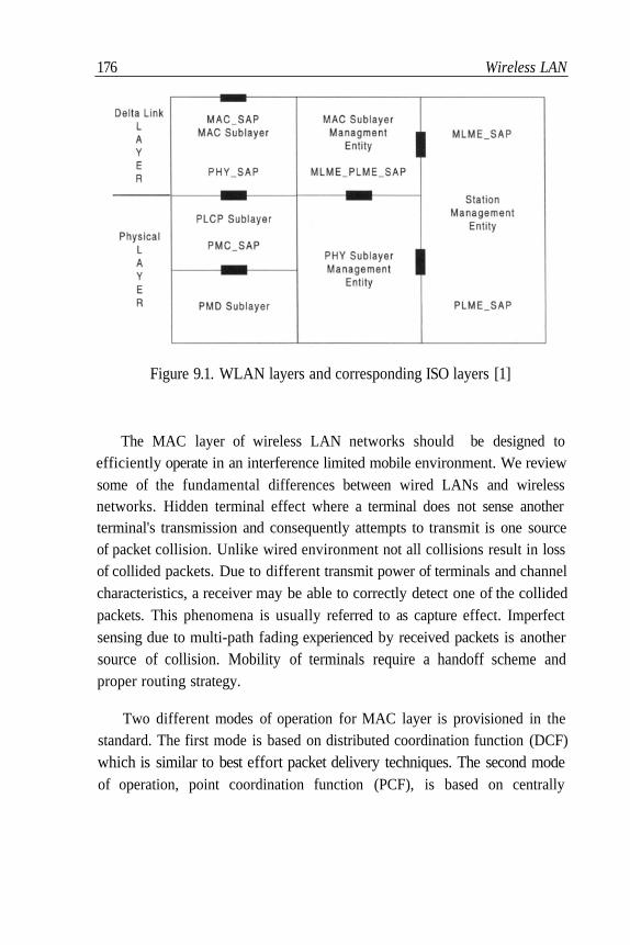
176 Wireless LAN
Figure 9.1. WLAN layers and corresponding ISO layers [1]
The MAC layer of wireless LAN networks should be designed toefficiently operate in an interference limited mobile environment. We reviewsome of the fundamental differences between wired LANs and wirelessnetworks. Hidden terminal effect where a terminal does not sense anotherterminal's transmission and consequently attempts to transmit is one sourceof packet collision. Unlike wired environment not all collisions result in lossof collided packets. Due to different transmit power of terminals and channelcharacteristics, a receiver may be able to correctly detect one of the collidedpackets. This phenomena is usually referred to as capture effect. Imperfectsensing due to multi-path fading experienced by received packets is anothersource of collision. Mobility of terminals require a handoff scheme andproper routing strategy.
Two different modes of operation for MAC layer is provisioned in thestandard. The first mode is based on distributed coordination function (DCF)which is similar to best effort packet delivery techniques. The second modeof operation, point coordination function (PCF), is based on centrally

Wireless LAN 177
controlled polling administered by access point (AP) and is used for delaysensitive data services.
Figure 9.2. MAC architecture [1].
Access points are connected to distribution systems which could beEthernet LAN, FDDI or other backbone infrastructure.
Figure 9.3. WLAN network architecture.
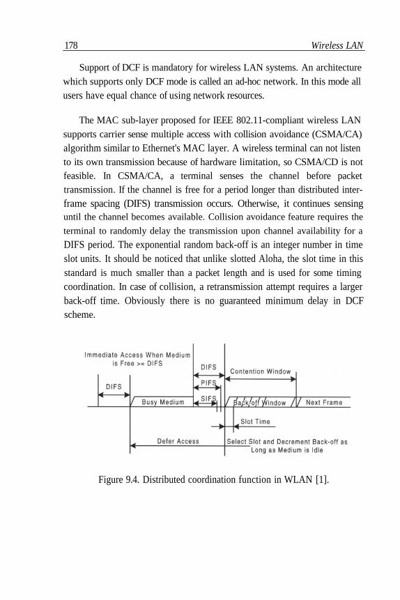
178 Wireless LAN
Support of DCF is mandatory for wireless LAN systems. An architecturewhich supports only DCF mode is called an ad-hoc network. In this mode allusers have equal chance of using network resources.
The MAC sub-layer proposed for IEEE 802.11-compliant wireless LANsupports carrier sense multiple access with collision avoidance (CSMA/CA)algorithm similar to Ethernet's MAC layer. A wireless terminal can not listento its own transmission because of hardware limitation, so CSMA/CD is notfeasible. In CSMA/CA, a terminal senses the channel before packettransmission. If the channel is free for a period longer than distributed inter-frame spacing (DIFS) transmission occurs. Otherwise, it continues sensinguntil the channel becomes available. Collision avoidance feature requires the
terminal to randomly delay the transmission upon channel availability for a
DIFS period. The exponential random back-off is an integer number in timeslot units. It should be noticed that unlike slotted Aloha, the slot time in thisstandard is much smaller than a packet length and is used for some timingcoordination. In case of collision, a retransmission attempt requires a largerback-off time. Obviously there is no guaranteed minimum delay in DCFscheme.
Figure 9.4. Distributed coordination function in WLAN [1].
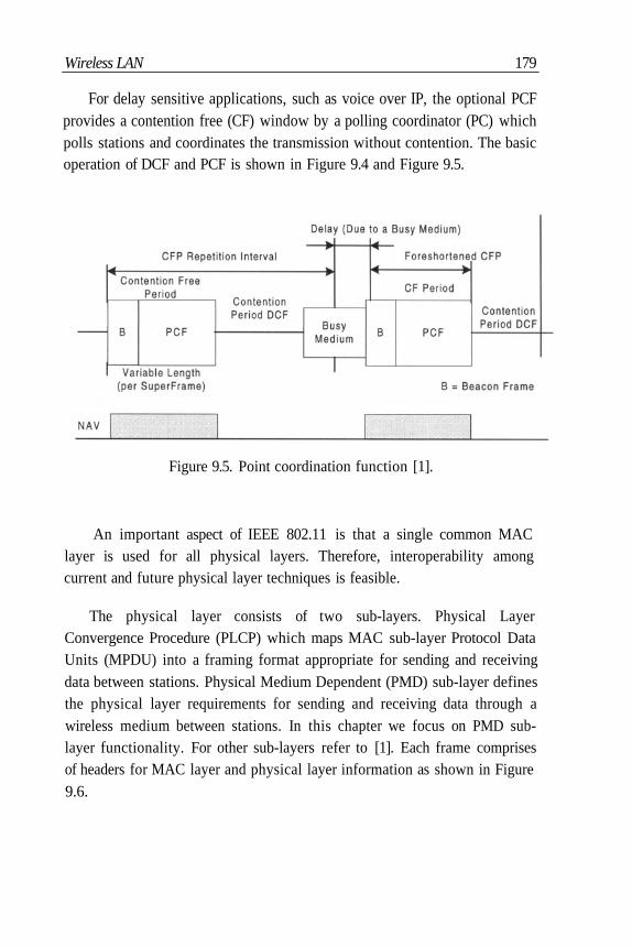
Wireless LAN 179
For delay sensitive applications, such as voice over IP, the optional PCFprovides a contention free (CF) window by a polling coordinator (PC) whichpolls stations and coordinates the transmission without contention. The basicoperation of DCF and PCF is shown in Figure 9.4 and Figure 9.5.
Figure 9.5. Point coordination function [1].
An important aspect of IEEE 802.11 is that a single common MAClayer is used for all physical layers. Therefore, interoperability amongcurrent and future physical layer techniques is feasible.
The physical layer consists of two sub-layers. Physical LayerConvergence Procedure (PLCP) which maps MAC sub-layer Protocol DataUnits (MPDU) into a framing format appropriate for sending and receivingdata between stations. Physical Medium Dependent (PMD) sub-layer definesthe physical layer requirements for sending and receiving data through awireless medium between stations. In this chapter we focus on PMD sub-layer functionality. For other sub-layers refer to [1]. Each frame comprisesof headers for MAC layer and physical layer information as shown in Figure9.6.
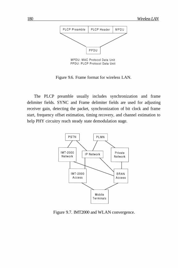
180 Wireless LAN
Figure 9.6. Frame format for wireless LAN.
The PLCP preamble usually includes synchronization and framedelimiter fields. SYNC and Frame delimiter fields are used for adjustingreceiver gain, detecting the packet, synchronization of bit clock and framestart, frequency offset estimation, timing recovery, and channel estimation tohelp PHY circuitry reach steady state demodulation stage.
Figure 9.7. IMT2000 and WLAN convergence.
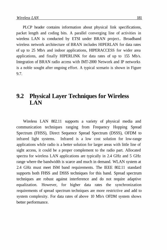
Wireless LAN 181
PLCP header contains information about physical link specifications,packet length and coding bits. A parallel converging line of activities inwireless LAN is conducted by ETSI under BRAN project.. Broadbandwireless network architecture of BRAN includes HIPERLAN for data ratesof up to 25 Mb/s and indoor applications, HIPERACCESS for wider areaapplications, and finally HIPERLINK for data rates of up to 155 Mb/s.Integration of BRAN radio access with IMT-2000 Network and IP networksis a noble sought after ongoing effort. A typical scenario is shown in Figure
9.7.
9.2 Physical Layer Techniques for WirelessLAN
Wireless LAN 802.11 supports a variety of physical media andcommunication techniques ranging from Frequency Hopping SpreadSpectrum (FHSS), Direct Sequence Spread Spectrum (DSSS), OFDM toinfrared light systems. Infrared is a low cost solution for low-rangeapplications while radio is a better solution for larger areas with little line ofsight access, it could be a proper complement to the radio part. Allocatedspectra for wireless LAN applications are typically in 2.4 GHz and 5 GHzrange where the bandwidth is scarce and much in demand. WLAN system at2.4 GHz must meet ISM band requirements. The IEEE 802.11 standardsupports both FHSS and DSSS techniques for this band. Spread spectrumtechniques are robust against interference and do not require adaptiveequalization. However, for higher data rates the synchronizationrequirements of spread spectrum techniques are more restrictive and add tosystem complexity. For data rates of above 10 Mb/s OFDM system showsbetter performance.
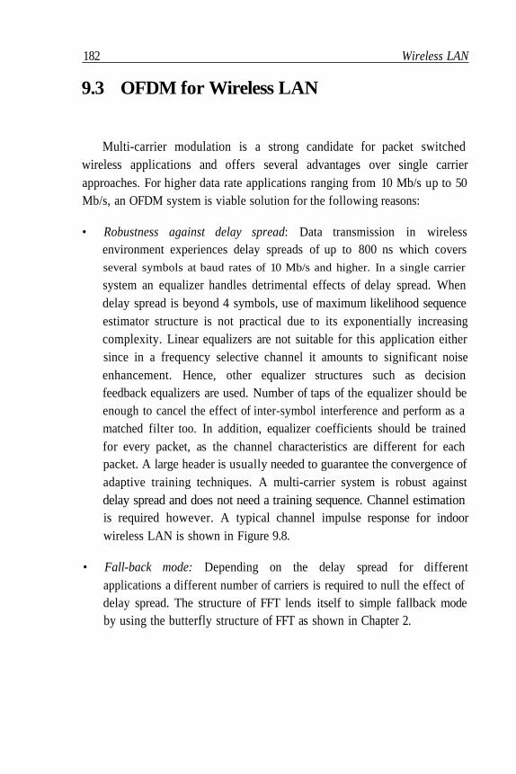
182 Wireless LAN
9.3 OFDM for Wireless LAN
Multi-carrier modulation is a strong candidate for packet switchedwireless applications and offers several advantages over single carrierapproaches. For higher data rate applications ranging from 10 Mb/s up to 50Mb/s, an OFDM system is viable solution for the following reasons:
• Robustness against delay spread: Data transmission in wirelessenvironment experiences delay spreads of up to 800 ns which coversseveral symbols at baud rates of 10 Mb/s and higher. In a single carrier
system an equalizer handles detrimental effects of delay spread. Whendelay spread is beyond 4 symbols, use of maximum likelihood sequenceestimator structure is not practical due to its exponentially increasingcomplexity. Linear equalizers are not suitable for this application eithersince in a frequency selective channel it amounts to significant noiseenhancement. Hence, other equalizer structures such as decisionfeedback equalizers are used. Number of taps of the equalizer should beenough to cancel the effect of inter-symbol interference and perform as amatched filter too. In addition, equalizer coefficients should be trainedfor every packet, as the channel characteristics are different for eachpacket. A large header is usually needed to guarantee the convergence ofadaptive training techniques. A multi-carrier system is robust againstdelay spread and does not need a training sequence. Channel estimationis required however. A typical channel impulse response for indoorwireless LAN is shown in Figure 9.8.
• Fall-back mode: Depending on the delay spread for differentapplications a different number of carriers is required to null the effect ofdelay spread. The structure of FFT lends itself to simple fallback modeby using the butterfly structure of FFT as shown in Chapter 2.

Wireless LAN 183
Figure 9.8. Channel impulse response for typical wireless LAN medium.
• Computational efficiency: Use of FFT structure at the receiver reduces
the complexity to N N . As the number of carriers grows the higher
efficiency can be achieved. A typical OFDM Wireless LAN is shown inthe Figure 9.9.
Figure 9.9. Wireless LAN system structure.

184 Wireless LAN
• Fast synchronization: OFDM receivers are less sensitive to timing jittercompared to spread spectrum techniques.
A typical OFDM wireless LAN transceiver is shown in Figure 9.9.
Transmitter Structure
WLAN system at 5 GHz supports variable data rates by using differentmodulation schemes and therefore requires variable coding gain for each
data rate. Currently, using BPSK, QPSK, 16 QAM and 64 QAM modulationsupports data rates of 6 Mb/s up to 54 Mb/s. Different coding rates forconvolutional coding are proposed depending on required protection
Obviously, more crowded constellations need higher coding protection.A combination of error detection, such as CRC, and error correction, such asconvolutional coding, in conjunction with interleaving are used to providebetter coding gain in the presence of frequency selective fading.Convolutional coding is usually punctured to provide higher bandwidthefficiency. The number of carriers and modulation of data bits depends onthe required data rates. Typical number of carriers is 48-52 and a guard bandis added to control the spectrum shape. Additional guard interval in the timedomain is used for pulse shaping and controlling the ISI. A typical frameformat of OFDM WLAN is shown in Figure 9.10.
Figure 9.10. Typical frame format for OFDM WLAN.
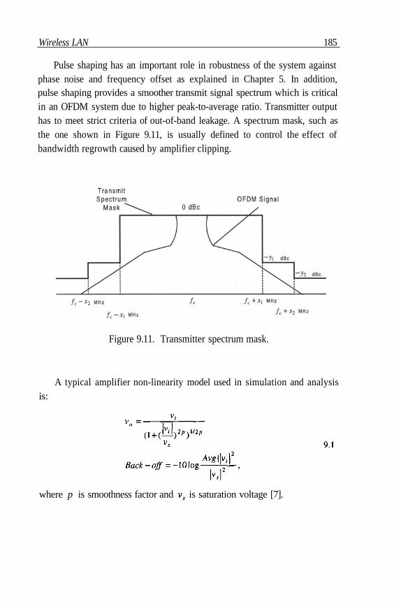
Wireless LAN 185
Pulse shaping has an important role in robustness of the system againstphase noise and frequency offset as explained in Chapter 5. In addition,pulse shaping provides a smoother transmit signal spectrum which is criticalin an OFDM system due to higher peak-to-average ratio. Transmitter outputhas to meet strict criteria of out-of-band leakage. A spectrum mask, such asthe one shown in Figure 9.11, is usually defined to control the effect ofbandwidth regrowth caused by amplifier clipping.
Figure 9.11. Transmitter spectrum mask.
A typical amplifier non-linearity model used in simulation and analysisis:
where p is smoothness factor and is saturation voltage [7].

186 Wireless LAN
Figure 9.12: Nonlinear HPA model
Some typical degradation factors at the transmitter are briefly discussedhere. Quadrature phase error and phase imbalance of transmitter modulationresult in a C/N degradation and higher packet error rate. Another source ofdegradation is the fixed-point error caused by truncating the output of IFFTbutterfly. After each stage of IFFT (or FFT) butterfly, the required numberof bits grows. Truncation of bits can also increase the packet error rate.Maximum tolerable transmitter degradation is restricted by vector error
requirements set forth in WLAN standards.
Currently, two frequency bands around 2.4 GHz and 5 GHz have beenassigned to wireless bands. Target data rates of up to about 50 Mb/s andhigher are also being considered for this system.
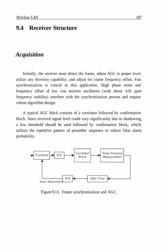
Wireless LAN 187
9.4 Receiver Structure
Acquisition
Initially, the receiver must detect the frame, adjust AGC to proper level,utilize any diversity capability, and adjust for coarse frequency offset. Fastsynchronization is critical in this application. High phase noise andfrequency offset of low cost receiver oscillators (with about 10 ppmfrequency stability) interfere with the synchronization process and requirerobust algorithm design.
A typical AGC block consists of a correlator followed by confirmationblock. Since received signal level could vary significantly due to shadowing,a low threshold should be used followed by confirmation block, whichutilizes the repetitive pattern of preamble sequence to reduce false alarmprobability.
Figure 9.13. Frame synchronization and AGC.
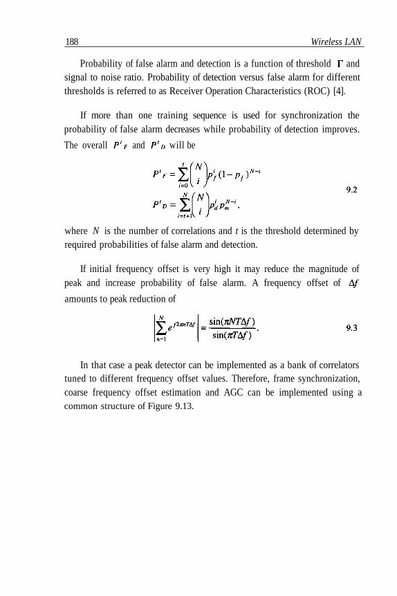
188 Wireless LAN
Probability of false alarm and detection is a function of threshold andsignal to noise ratio. Probability of detection versus false alarm for differentthresholds is referred to as Receiver Operation Characteristics (ROC) [4].
If more than one training sequence is used for synchronization theprobability of false alarm decreases while probability of detection improves.
The overall and will be
where N is the number of correlations and t is the threshold determined byrequired probabilities of false alarm and detection.
If initial frequency offset is very high it may reduce the magnitude ofpeak and increase probability of false alarm. A frequency offset of
amounts to peak reduction of
In that case a peak detector can be implemented as a bank of correlatorstuned to different frequency offset values. Therefore, frame synchronization,coarse frequency offset estimation and AGC can be implemented using acommon structure of Figure 9.13.
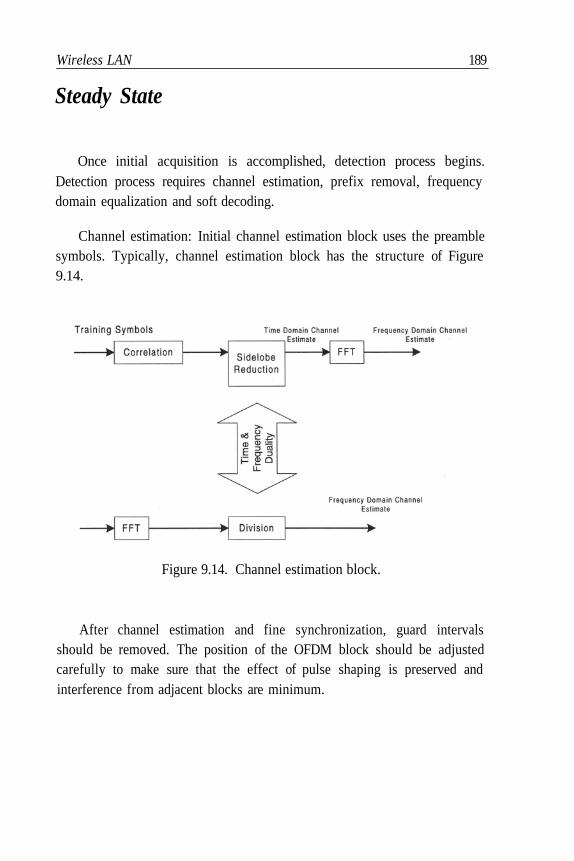
Wireless LAN 189
Steady State
Once initial acquisition is accomplished, detection process begins.Detection process requires channel estimation, prefix removal, frequencydomain equalization and soft decoding.
Channel estimation: Initial channel estimation block uses the preamblesymbols. Typically, channel estimation block has the structure of Figure9.14.
Figure 9.14. Channel estimation block.
After channel estimation and fine synchronization, guard intervalsshould be removed. The position of the OFDM block should be adjustedcarefully to make sure that the effect of pulse shaping is preserved andinterference from adjacent blocks are minimum.

190 Wireless LAN
Using a reliability index concept performs soft decoding of thedemodulated signal. Due to the presence of an interleaver block a classictrellis decoding is not possible. We correspond a reliability parameter toeach bit and use that in decoding. The reliability index for each bit is derivedfrom the difference in metric value caused by bit flipping.
Typical degradation sources in the receiver are phase noise of the localoscillator, which was thoroughly discussed in previous chapters, and D/Aquantization error. Overall, transmitter power amplifier non-linearity andreceiver phase noise are dominant factors for total vector error.
References
1. IEEE. "IEEE Standard 802.11, Part 11: Wireless LAN Medium Access Control (MAC)and Physical Layer (PHY) Specifications." Piscataway, NJ: IEEE, 1997.
2. Draft Supplement to Standard for Telecommunication and Information ExchangeBetween Systems-LAN/MAN Specific Requirements-Part 11: Wireless Medium AccessControl (MAC) and Physical Layer (PHY) Specifications. High Speed Physical Layer inthe 5 GHz Band. Sept., 1998
3. Stallings, W. Data and Computer Communications. New York: Maxwell MacMillan,1991.
4. Helstrom, C. W. Statistical Theory of Signal Detection. London: Pergamon, 1966.
7. Bahai, A.R.S. “Estimation in Randomly Time-Varying Systems with Applications toDigital Communications.” Ph.D. Dissertation, Univ. of California at Berkeley, 1993.
5. Viterbi, A.J. CDMA, Principles of Spread Spectrum Communication Reading, MA:Addison Wesley, 1995.
6. Takanashi, H. "Proposal of PHY Specification for 5 GHz Band." Proposal to IEEE802.11 Committee, Jan 1998.
7. Bogenfeld, E, et al. "Influence of Nonlinear HPA on Trellis-Coded OFDM for TerrestrialBroadcasting of Digital." IEEE Proc. of Global Telecom Conf. (GLOBECOM '93);1433-1438.

Chapter 10 Digital Broadcasting
10.1 Broadcasting of Digital Audio Signals
It has been recognized, particularly in Europe, that multi-carriermodulation is especially appropriate for broadcasting of digital signals.European standards bodies have adopted OFDM as the modulation choicefor several variations of digital audio and digital television, for bothterrestrial and satellite transmission [1-3]. We will concentrate here on oneparticularly interesting form of terrestrial digital audio broadcasting.
Substantial quality improvement can be obtained over conventionalanalog FM by using digital techniques, just as digital compact disk (CD)recording has widely supplanted analog disks and tapes. With moderncompression techniques, high quality stereo audio can be produced atapproximately 200 kb/s, an order of magnitude reduction from CDtechnology, which uses a straight PCM encoding without compression.
The European Digital Audio Broadcast (DAB) standard provides forthree modes of operation. Mode 1 is for terrestrial Single FrequencyNetworks (SFN). Mode 2 applies to conventional terrestrial localbroadcasting. Mode 3 is for satellite broadcasting. The ability to provide an
191

192 Digital Broadcasting
SFN is a unique capability of multi-carrier modulation, and the remainder ofthis section will discuss this application.
An SFN involves the provision of several geographically dispersedtransmitters, all transmitting the same signal, synchronized in time. Thispermits coverage of a large area, and also fills in dead spots due toshadowing at a particular receiver location. Any receiver therefore receives asum of signals from more than one transmitter, coincident in frequency,format, and time, except for differences in propagation delay. This is
illustrated in Figure 10.1, showing multi-path propagation from several
transmitters.
Figure 10.1. Received signal in an SFN.
Assuming that each path provides a Rayleigh distributed signal, thepowers will add. If the spread of arrival times, which includes both multi-path spread and spread of propagation times from different transmitters, isless than the guard interval between OFDM symbols, then orthogonalityamong sub-carriers is preserved. If this is not the case, then degradation
caused by interference among sub-carriers will result. This interference maybe approximated as Gaussian noise, and is proportional to the degree that theinter-symbol interference duration exceeds the guard interval. As an exampleof a guard interval requirement, consider a receiver receiving direct signals

Digital Broadcasting 193
from two transmitters 40 km apart. The time separation of the signals could
be up to 133 sec. Considering the addition of multi-path from each
transmitter, and reception from additional transmitters, the guard intervalshould be substantially greater than this value. Note that as in a cellular radio
system, signals from far distant transmitters lead to system degradation.
A constraint in the other direction, due to Doppler shift and frequencyvariation in the receiver's local oscillator, sets a minimum spacing betweensub-carriers, and thus a maximum symbol duration. For a vehicle travellingat 80 mph (31 m/s), the Doppler shift at 240 MHz can be up to 25 Hz. Thesub-carrier spacing must be large compared to this value in order to
minimize this source of inter-carrier interference. It is particularly importantin an OFDM system that a good frequency lock be maintained in thereceiver.
The Mode 1 standard meets these constraints by providing for 1536 sub-carriers with 1 kHz spacing. A guard interval, which employs a cyclic prefix,has a duration of 246 sec.
Since the useful symbol duration is 1 msec, the loss in spectralefficiency is approximately 20%. Each sub-carrier is modulated by /4-
DPSK, that is a 4-point constellation in which two bits of information are
carried by differential phase modulation of
A 2048-point IFFT is performed in the transmitter, treating the unusedsub-carriers as zero, so the bandwidth remains 1.536 MHz. The signal iscomplex modulated, using I and Q components, onto an RF carrier in therange 175 - 240 MHz.
The transmitted OFDM signal carries several audio programs, each ofwhich may be monophonic or stereo, and of varying quality. Each audio
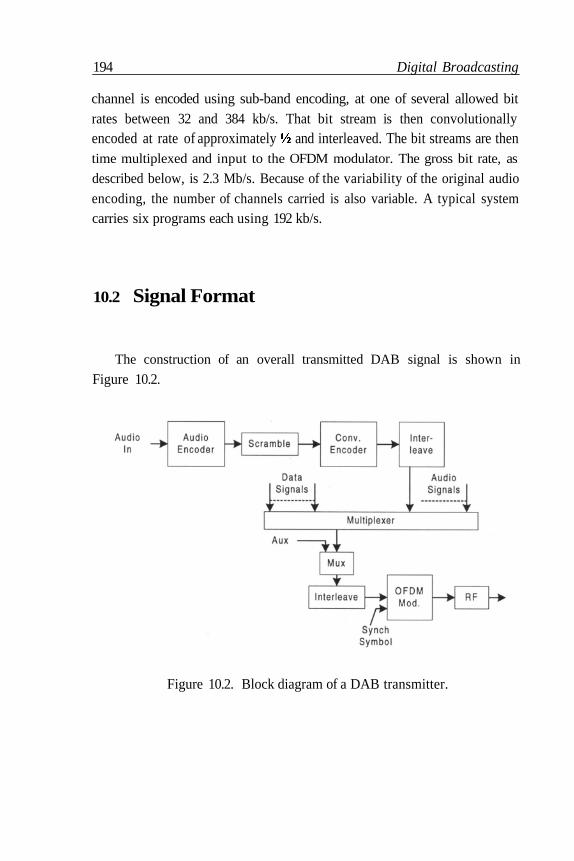
194 Digital Broadcasting
channel is encoded using sub-band encoding, at one of several allowed bitrates between 32 and 384 kb/s. That bit stream is then convolutionallyencoded at rate of approximately and interleaved. The bit streams are thentime multiplexed and input to the OFDM modulator. The gross bit rate, as
described below, is 2.3 Mb/s. Because of the variability of the original audioencoding, the number of channels carried is also variable. A typical systemcarries six programs each using 192 kb/s.
10.2 Signal Format
The construction of an overall transmitted DAB signal is shown in
Figure 10.2.
Figure 10.2. Block diagram of a DAB transmitter.
Digital Broadcasting 195
The audio encoder accepts digital samples of the audio input, which in
general is 2-channel stereo. The samples occur at a 48 kHz. rate, 16 bits persample, for a total rate of 768 kb/s. per channel. A sub-band encodingtechnique is used to reduce the rate to a lower value, depending on thedesired subjective quality.
The output of the audio encoder is scrambled by modulo-2 addition with
a pseudo-random sequence formed from a 9-bit feedback shift register. Thisis different from the more common scrambling technique of division by arandomizing polynomial. It does not suffer from error multiplication effects,but does require synchronization of the descrambling sequence at thereceiver. The purpose of this scrambling is to insure that the final transmitted
frequency spectrum is suitable dispersed. In addition, the standard allows foradditional encryption scrambling if appropriate.
The scrambled data is then convolutionally encoded. This is essential forsatisfactory operation over a radio channel. The first step is a mother code ofrate with constraint length 7. That code is then subjected to puncturing toyield a rate of the form 8/n, where n can be any integer value between 9 and32. Each audio channel can have a different code rate, depending on therequired error rate, to produce a given audio quality over the expected worstcase channel. Typically a rate of approximately is used. Interleaving by a
factor of 16 is then applied.
Several audio channels are multiplexed and combined with other signals,which may include data channels in addition to audio. The signals arearranged in frames, as shown below. A frame consists of a time sequence of2 synchronization symbols, 3 digital overhead symbols, followed by 72symbols of multiplexed audio information. A symbol is a block of 3072 bitswhich will be mapped into an OFDM symbol. The length of a frame istherefore 77* 1.246 96 msec.
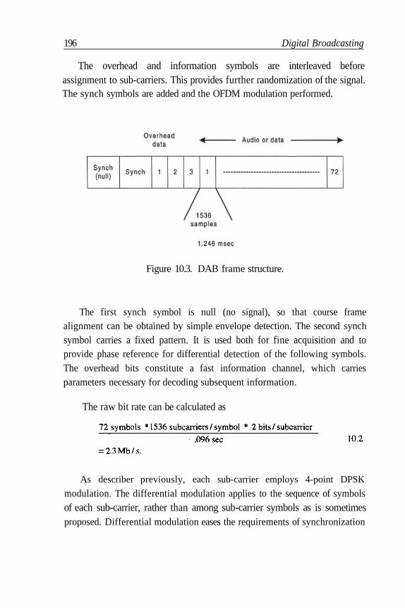
196 Digital Broadcasting
The overhead and information symbols are interleaved beforeassignment to sub-carriers. This provides further randomization of the signal.The synch symbols are added and the OFDM modulation performed.
Figure 10.3. DAB frame structure.
The first synch symbol is null (no signal), so that course framealignment can be obtained by simple envelope detection. The second synchsymbol carries a fixed pattern. It is used both for fine acquisition and toprovide phase reference for differential detection of the following symbols.The overhead bits constitute a fast information channel, which carriesparameters necessary for decoding subsequent information.
The raw bit rate can be calculated as
As describer previously, each sub-carrier employs 4-point DPSK
modulation. The differential modulation applies to the sequence of symbolsof each sub-carrier, rather than among sub-carrier symbols as is sometimesproposed. Differential modulation eases the requirements of synchronization

Digital Broadcasting 197
and simplifies receiver implementation, at the expense of approximately 2dB in noise performance. For satisfactory performance, the OFDM symbolrate must be large compared to the maximum Doppler shift. An equivalentstatement is that the OFDM symbol duration must be small compared to thetime coherence of the channel.
10.3 Other Digital Broadcasting Systems
DAB in the U.S.A.
The system requirements for DAB in the U.S.A. are considerablydifferent from those in Europe. Most importantly, it is desired to operate inthe same 88 – 108 MHz band that is used for conventional analog FMbroadcasting, using the same 200 kHz channels. This leads to a potentiallysevere problem of co-channel and adjacent channel interference between thedigital and analog signals.
The problem of interference from the digital signals into analogreceivers in reduced by transmitting the digital signals at a much lowerpower level than the analog signals. The FM capture effect then assists inrejection of the interference. Careful geographic frequency assignment andco-ordination is essential.
As for reception of the digital signal, interference from analog stations isa form of additive noise. Robust signal format and coding are essential. Onesuggested enhancement involves detecting an analog interferer andattempting to subtract it out [4, 5].
198 Digital Broadcasting
Standardization of the signal format is in progress, but some form ofOFDM will most likely be adopted.
A standard similar to the DAB standard has been adopted in Europe forbroadcasting of digital television signals. Using MPEG-2 coding,approximately 3 – 4 Mb/s are required for high quality SECAM or PALprogramming, while up to 20 Mb/s are needed for future high definitiontelevision.
A bandwidth of 8 MHz is used, as in PAL or SECAM, to carry eitherseveral standard channels or one high definition channel. The same SFNscheme as in DAB will be deployed. In this case 8000 sub-carriers spacedapproximately 1 kHz apart are used. Larger constellation sizes, up to 64points, provide the higher bit rates.
The large constellation sizes require more robust techniques than are
used in DAB [6, 7]. Modulation is coherent as opposed to differential. Aconcatenated inner convolution code and outer block code are employed.Several pilot tones are transmitted for more precise equalization andsynchronization.
10.4 Digital Video Broadcasting
Digital video broadcasting services cover more than digital television.The wireless video concept includes applications such as multimedia mobileand wireless data services. In addition, DVB systems can be integrated withother wireless services such as cellular systems to provide a highly
asymmetric data access system which is desirable for new wireless Internet
access.
Digital Broadcasting 199
Source coding is one of the most critical components of DVB systems.
Different data rates are required for the variety of services offered by DVB.Quality television requires about 216 Mb/s and stereo audio requires about1536 kb/s with no source coding applied. MPEG 2 utilizes a compressionalgorithm to remove spatial, temporal and statistical redundancy of images,and sub-band coding techniques in conjunction with psycho-acoustic modelsto reduce the bit rate. The total bit rate, video and audio is reduced toapproximately 3.5 Mb/s.
The choice of Coded Orthogonal Frequency Division Multiplexing(COFDM) for DVB-T applications is based on several design factors:
• Interference rejection: Co-existence of digital broadcasting systems withcurrent analoge services requires a system design which restrictsinterference into analoge systems and is robust against narrow bandinterference. The former can be met by reducing power level andutilizing coding techniques of digital communications to achieverequired bit error rates. The latter can be met by multi-carrier modulationefficiently due to its robustness against narrow band interference such asVSB-AM.
• Multi-path effect: Multi-path propagation is a major impairment of aterrestrial broadcasting channel. The SFN architecture of DVB producesstrong echo ( 0 dB) generated by adjacent transmitters. Presence ofstrong echo-like interference requires a robust modulation scheme.COFDM is again suitable to combat against strong multi-path as long asthe guard interval length is properly designed. Larger guard intervals, asexplained before, allows larger distance between transmitters at theexpense of reduced bandwidth utilization. Proper positioning of pilotsignals in time and frequency slots provides an acceptable performancein higher Doppler conditions such as mobile multimedia terminals.

200 Digital Broadcasting
Figure 10.4. DVB transmitter structure.
After down conversion at the receiver's analog front-end and sampling, adigital AGC is used to adjust the VGA gain in the front-end circuit. A coarsefrequency offset correction is necessary to reduce the inter-carrierinterference. Frequency offset estimation uses the fixed pilots for initialestimation and scattered pilots for further fine synchronization. Timesynchronization is initially performed by using a correlator structure andfurther refinement is done by methods explained in Chapter 5 for finesynchronization using the output of the OFDM demodulator. Channelestimation is required for detection and soft decoding reliability measure.Pilot symbols are used for channel estimation, and by using time andfrequency interpolation we can obtain a channel estimate for all sub-carriersadaptively. Performance of the inner decoder is significantly enhanced byusing a soft decoder and a reliability measure derived from channel
estimation. A typical receiver is shown in Figure 10.5.
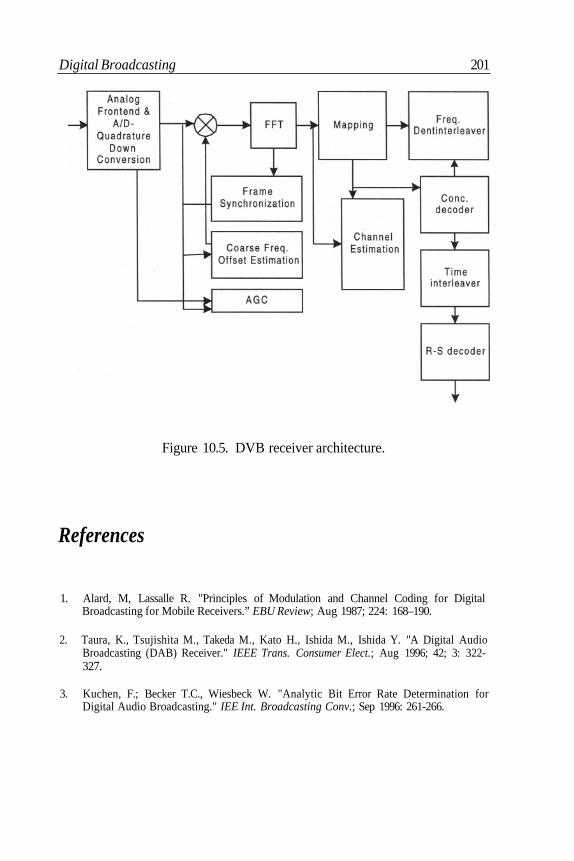
Digital Broadcasting 201
Figure 10.5. DVB receiver architecture.
References
1. Alard, M, Lassalle R. "Principles of Modulation and Channel Coding for DigitalBroadcasting for Mobile Receivers.” EBU Review; Aug 1987; 224: 168–190.
2. Taura, K., Tsujishita M., Takeda M., Kato H., Ishida M., Ishida Y. "A Digital AudioBroadcasting (DAB) Receiver." IEEE Trans. Consumer Elect.; Aug 1996; 42; 3: 322-327.
3. Kuchen, F.; Becker T.C., Wiesbeck W. "Analytic Bit Error Rate Determination forDigital Audio Broadcasting." IEE Int. Broadcasting Conv.; Sep 1996: 261-266.
202 Digital Broadcasting
4. Leclerc, M, Scalart P., Fautier P., Huynh H.T. "Performance Analysis of an In-BandCOFDM/FM Digital Audio Broadcasting System." IEEE Trans. Broadcasting; Jun 1997;43; 2: 191-198.
5. Kroeger, B.W., Peyla P.J. "Compatibility of FM Hybrid In-Band On-Channel (IBOC)System for Digital Audio Broadcasting." IEEE Trans. Broadcasting; Dec 1997; 43; 4:421-430.
6. Mignone, V., Morello A., Visintin M. "An Advanced Algorithm for Improving DVB-TCoverage in SFN." IEEE Int. Broadcasting Conv.; Sep 1997: 534-540.
7. Sari, H., Karam G., Jeanclaude I. "Transmission Techniques for Digital Terrestrial TVBroadcasting." IEEE Commun. Mag.; Feb 1995; 33; 2: 100-109.
Chapter 11 Future Trends
Multi-carrier communications are currently in a state of very rapiddevelopment, both in the introduction of new techniques and in applicationto a wide variety of channels and services. Advances in algorithmicdevelopment and in the capabilities of signal processing devices will surelylead to substantial improvement in performance of multi-carrier systems.This in turn will lead to further application in systems where the uniqueadvantages of multi-carrier modulation can be applied, while overcoming itsdrawbacks, at reasonable cost.
11.1 Comparison with Single CarrierModulation
In Reference [1] a comparison was made of the relative advantages ofOFDM and single carrier modulation in the ADSL application. The tablebelow indicates which system is favored for each of several issues.
203

204 Future Trends
The comparisons also apply for environments other than ADSL. Asshown in Chapter 3, bandwidth efficiency and performance in the presence
of colored Gaussian noise ideally are equal, if the single carrier system usesoptimum decision feedback equalization and the multi-carrier systememploys optimum bit loading. The relative computation per unit time is lessfor multi-carrier in the ADSL environment where the long equalizer neededto correct the highly dispersive channel response in a single carrierimplementation requires more computation than the short equalizer and FFTin multi-carrier. The higher cost and power drain of analog components formulti-carrier, particularly the transmitter power amplifier, results from thenecessity to keep clipping at a minimum. The sensitivity to narrowband
Table 1: Relative advantages of single carrier and multi-carrier modulation.An "X" denotes the system with better performance or lower cost.
Future Trends 205
noise and jitter are due to the overlapping and slowly decaying sub-carrierspectra in multi-carrier modulation.
Future enhancements to OFDM give promise of reversing some of thecases in which OFDM compares unfavorably, in particular those associatedwith clipping and the overlapping sub-carrier spectra in current OFDMimplementations.
11.2 Mitigation of Clipping Effects
In Chapter 4 it was shown that the error probability resulting fromclipping may be quite tolerable in most cases. However the need to limit thecost, and even more importantly the power drain, of components such as the
transmitter power amplifier provides an incentive to keep the peak-to-average power ratio as small as possible. Several approaches have beenproposed to accomplish this.
Probably the simplest solution is to allow clipping at a relatively lowlevel, and use standard error control coding to correct the resultant errors. Ofcourse this also reduces errors caused by other degradations, in particularadditive noise. In [2] it is shown that this simple approach may comparefavorably with other techniques when the clipping level is not reduced to toolow a value. Another receiving scheme involves attempting to reconstructthe clipped signal [3].
A large number of proposals involve altering the transmitted signal so asto keep the peak value low, and in most cases notifying the receiver of thealteration. Because the probability of a clip is relatively low in any case, theside information required to perform this notification can be quite lowcompared with the actual data [4]. One relatively simple approach is tobuffer each OFDM symbol before transmission and to detect if the clipping
206 Future Trends
level would be exceeded. If so, the level is reduced and the reported to thereceiver, possibly on a sub-carrier dedicated to this purpose.
Other techniques [5, 6, 7] use block codes to produce more than one
mapping of input data to OFDM symbols, and transmit the one with lowestpeak. The mappings typically involve different rotations of the sub-carrierconstellations. Side information is sent to the receiver as before to reportwhich mapping was used. In practice only one or two bits of sideinformation per OFDM symbol are needed. If unused sub-carriers are
available, then they could be modulated in a way that reduces the peak valueof each OFDM symbol. In this case no side information need be transmittedbecause those sub-carriers are ignored in any case.
In Reference [6], it is shown that that for an error probability of thepeak-to-average ratio can be reduced from 13.3 dB to 11.1 dB by the use of
two mappings, or down to 9.5 dB with four mappings.
Reduction of the peak value of an OFDM signal is now an active field ofresearch, involving trade-offs among performance, spectral efficiency, andcomplexity of implementation. Incorporation of some of these techniques incertain applications of OFDM may be expected in the near future.
11.3 Overlapped Transforms
When the time window used in modulation is a square one equal to theOFDM symbol duration, the spectrum of each sub-carrier is of the sinc form.
Each sub-carrier spectrum therefore overlaps many of the others. This leadsto high inter-channel interference when orthogonality is lost for any reason,such as inter-symbol interference, frequency offset, or phase noise. Inaddition, the susceptibility to narrow-band interference can be severe in thatmany sub-channels could be affected by a single interferer. The problem can

Future Trends 207
partially be relieved by the use of windowing as described in Chapter 2.However there is only the duration of the cyclic prefix to provide room forthe window shaping, so that substantial overlap of sub-carrier spectra willremain.
Much better spectral shaping can be achieved if processing is no longerconstrained to the duration of a block corresponding to a single OFDMsymbol. If several blocks are allowed to overlap in time, then a very gradualwindowing function can be introduced. Reference [8] describes theperformance that can be achieved by a technique called Discrete WaveletMulti-Tone (DWMT) modulation. In particular, for an overlap of 8 blocks,the first sidelobe of each sub-carrier spectrum is reduced from -13.5 dB inDMT to -45 dB. Performance in noise is substantially unchanged, andsensitivity to various inaccuracies is greatly reduced. Furthermore, no cyclicprefix is needed, leading to maximum spectral efficiency. However DWMTrequires substantially greater computational complexity, and latency isincreased by the degree of overlap. The DWMT transmitter is shown inFigure 11.1.
Figure 11.1. DWMT transmitter.
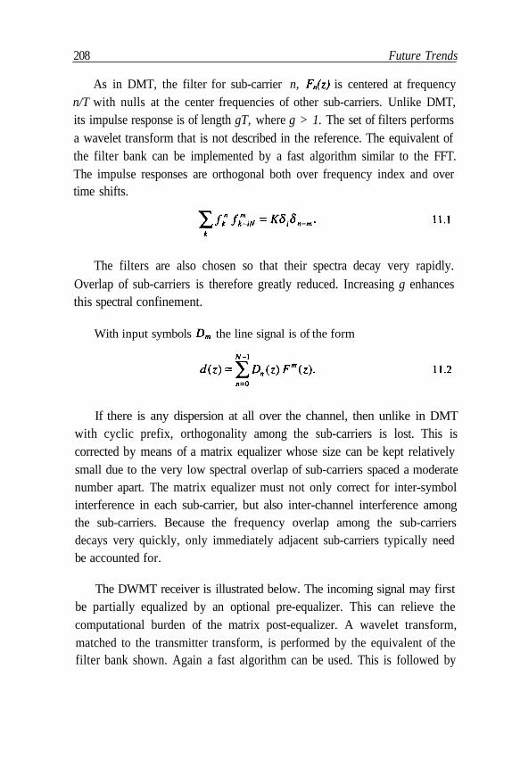
208 Future Trends
As in DMT, the filter for sub-carrier n, is centered at frequencyn/T with nulls at the center frequencies of other sub-carriers. Unlike DMT,its impulse response is of length gT, where g > 1. The set of filters performsa wavelet transform that is not described in the reference. The equivalent ofthe filter bank can be implemented by a fast algorithm similar to the FFT.The impulse responses are orthogonal both over frequency index and overtime shifts.
The filters are also chosen so that their spectra decay very rapidly.Overlap of sub-carriers is therefore greatly reduced. Increasing g enhancesthis spectral confinement.
With input symbols the line signal is of the form
If there is any dispersion at all over the channel, then unlike in DMTwith cyclic prefix, orthogonality among the sub-carriers is lost. This iscorrected by means of a matrix equalizer whose size can be kept relativelysmall due to the very low spectral overlap of sub-carriers spaced a moderatenumber apart. The matrix equalizer must not only correct for inter-symbolinterference in each sub-carrier, but also inter-channel interference amongthe sub-carriers. Because the frequency overlap among the sub-carriersdecays very quickly, only immediately adjacent sub-carriers typically needbe accounted for.
The DWMT receiver is illustrated below. The incoming signal may firstbe partially equalized by an optional pre-equalizer. This can relieve thecomputational burden of the matrix post-equalizer. A wavelet transform,matched to the transmitter transform, is performed by the equivalent of thefilter bank shown. Again a fast algorithm can be used. This is followed by
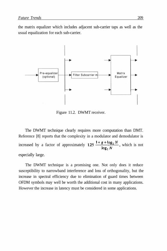
Future Trends 209
the matrix equalizer which includes adjacent sub-carrier taps as well as theusual equalization for each sub-carrier.
Figure 11.2. DWMT receiver.
The DWMT technique clearly requires more computation than DMT.Reference [8] reports that the complexity in a modulator and demodulator is
increased by a factor of approximately which is not
especially large.
The DWMT technique is a promising one. Not only does it reducesusceptibility to narrowband interference and loss of orthogonality, but theincrease in spectral efficiency due to elimination of guard times betweenOFDM symbols may well be worth the additional cost in many applications.However the increase in latency must be considered in some applications.
210 Future Trends
11.4 Combined CDMA and OFDM
Several proposals have been made to combine the use of CDMA forwireless multiple access with the desirable properties of OFDM [9, 10]. Thelonger symbol interval in OFDM greatly eases the problem of acquiringsynchronization of the spreading code in the receiver. The sub-carriers arespaced sufficiently close such that each sub-carrier constitutes a frequencynon-selective fading channel. This eliminates the need for RAKE combining.
Figure 11.3 shows one scheme. The same data symbol, multiplied by a
different bit of the spreading code {c}, modulates each sub-carrier. This in
effect provides spreading in the frequency domain. The transmitted signalelement duration is the same as the original symbol duration, rather than thechip duration as in ordinary CDMA. Synchronization is therefore a muchsimpler process. Provided that adequate guard intervals, using cyclicprefixes, are used, multi-path correction is easier and better than RAKEcombining in a single carrier system. This OFDM-CDMA techniqueprovides frequency diversity. Best performance in this environment isachieved through the use of optimum combining in the choice of weightingfactors {q} that are applied in the receiver after demodulation and
despreading.
In the downstream direction (from a central station to the mobile)multiple access is achieved by superimposing signals for different users onthe same sub-carriers using a set of orthogonal spreading codes such asWalsh functions. In the upstream direction a set of spreading codes, such asGold codes, with good auto-correlation and cross-correlation properties, areemployed. However in this case a multi-user detection scheme in thereceiver is essential because the asynchronous arrival times destroy
orthogonality among the OFDM sub-carriers.
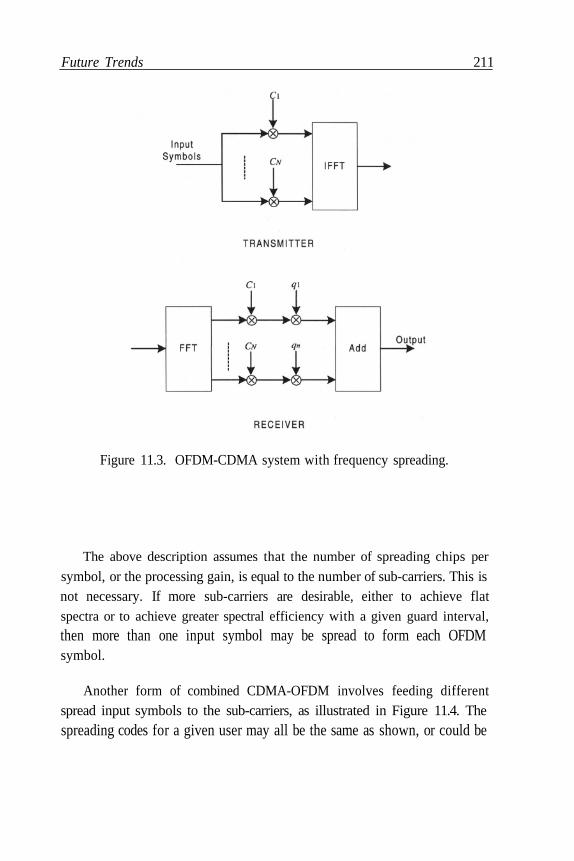
Future Trends 211
Figure 11.3. OFDM-CDMA system with frequency spreading.
The above description assumes that the number of spreading chips per
symbol, or the processing gain, is equal to the number of sub-carriers. This isnot necessary. If more sub-carriers are desirable, either to achieve flatspectra or to achieve greater spectral efficiency with a given guard interval,
then more than one input symbol may be spread to form each OFDMsymbol.
Another form of combined CDMA-OFDM involves feeding differentspread input symbols to the sub-carriers, as illustrated in Figure 11.4. Thespreading codes for a given user may all be the same as shown, or could be
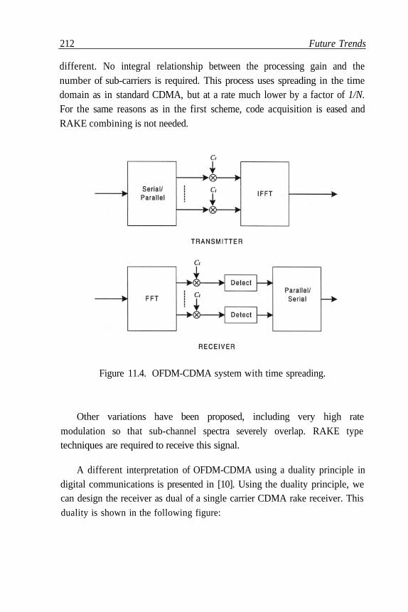
212 Future Trends
different. No integral relationship between the processing gain and thenumber of sub-carriers is required. This process uses spreading in the timedomain as in standard CDMA, but at a rate much lower by a factor of 1/N.For the same reasons as in the first scheme, code acquisition is eased andRAKE combining is not needed.
Figure 11.4. OFDM-CDMA system with time spreading.
Other variations have been proposed, including very high rate
modulation so that sub-channel spectra severely overlap. RAKE typetechniques are required to receive this signal.
A different interpretation of OFDM-CDMA using a duality principle indigital communications is presented in [10]. Using the duality principle, wecan design the receiver as dual of a single carrier CDMA rake receiver. Thisduality is shown in the following figure:

Future Trends 213
Figure 11.5. Discrete time MC-SS rake in frequency domain.
Figure 11.6. Simplified rake receiver.
11.5 Advances in Implementation
"Moore's Law" concerning the exponential increase in the number ofelements that can be included on a chip is expected to hold for the next fewyears. One consequence will be the availability of general purpose signalprocessing chips that can perform advanced algorithms for fairly high rateOFDM systems. Another is the availability of circuitry that is dedicated toperforming common functions efficiently, either as part of a signalprocessing chip or as an auxiliary chip. Functions now available includeFFTs, Viterbi decoders, Reed-Solomon coders and decoders, etc.

214 Future Trends
Implementation of the butterfly operation of FFT in a modern DSP issignificantly more efficient than before. Execution of a 1024-point bitreversed complex Fast Fourier Transform in a new DSP takes less than 50microseconds.
Analog/Digital converters have been critical components in terms of costin the past. Because of the high peak-to-average ratio of OFDM signals, thishas been a serious issue for such systems. However recent advances in signalconversion devices have reduced this concern. Availability of high speedA/D devices with high spurious-free dynamic range (SFDR) and signal-to-noise ratio (SNR) at reasonable cost has resulted in further research anddevelopment in Digital Radio architecture. By using a combination of highspeed A/D and digital down conversion, complexity of an analog front-endis reduced and the system architecture is more flexible. Programmability ofdigital radio is an attractive feature for multi-mode and multi-band wirelessapplication.
Figure 11.7. IF sampling and digital radio down conversion.
Future Trends 215
Characteristics of power amplifiers are important for OFDM systemphysical layer performance such as bit error rate level, as discussed inChapter 4, and for power consumption requirements. Power amplifiers arethe largest source of battery drain in wireless systems. Recent advances inGaAs MMIC has resulted in highly efficient wideband power amplifierssuitable for OFDM applications.
References
1. Saltzberg, B.R. "Comparison of Single Carrier and Multitone Digital Modulation forADSL Applications." IEEE Commun. Magazine; Nov 1988; 36; 11: 114-121.
2. Wulich, D., Goldfeld L. “Reduction of Peak Factor in Orthogonal MulticarrierModulation by Amplitude Limiting and Coding.” IEEE Trans. Commun.; Jan 1999; 47:18-21.
3. Kim, D., Stuber S.L. “Clipping Noise Mitigation for OFDM by Decision-AidedReconstruction.” IEEE Commun. Let.; Jan 1999; 3; 1: 4–6.
4. Starr, T., Cioffi J.M., Silverman P. Understanding Digital Subscriber Line Technology.Upper Saddle River, NJ: Prentice Hall, 1999, 236-242.
5. Mestdagh, D.J.G., Spruyt P.M.P. "A Method to Reduce the Probability of Clipping inDMT-Based Transceivers." IEEE Trans. Commun.; Oct 1996; 44: 1234-1238.
6. Baum, R. W., Fischer R. F. H., Huber J. B. “Reducing the Peak-to-Average Ratio ofMulticarrier Modulation by Selective Mapping.” Electronic Letters; Oct 1996; 32: 2056-2057.
7. Shepard, S., Orriss J., Barton S. "Asymptotic Limits in Peak Envelope Reduction byRedundancy Coding in OFDM Modulation." IEEE Trans. Commun.; Jan 1998; 46: 5-10.
8. Sandberg, S.D., Tzannes M.A. "Overlapped Discrete Multitone Modulation for HighSpeed Copper Wire Communication." IEEE J. on Sel. Areas in Commun.; Dec 1995;SAC-13; 9: 1571-1585.
9. Hara, S., Prasad R. "Overview of Multicarrier CDMA." IEEE Commun. Magazine; Dec1997; 35; 12: 126-133.

216 Future Trends
10. Bahai, A., Fettwies G." Results on MC-CDMA Receiver Design." IEEE Int’l Conf.Comm; Jun 1995: 915-918.