Multi-attribute utility theory - Utrecht University · Multi-attribute utility theory (very superﬁcial in textbook!) 164 / 401 Multiple objectives – an example Consider the problem

Multi-attribute utility theory(very superficial in textbook!)

164 / 401

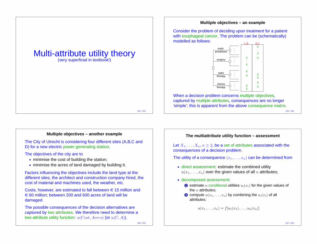
Multiple objectives – an example

Consider the problem of deciding upon treatment for a patientwith esophageal cancer. The problem can be (schematically)modelled as follows:

radiotherapy

chemotherapy

surgery

endoprosthesis

L.E. Q.L.X

X

X

X

X

X

X XX

X

XXX

When a decision problem concerns multiple objectives,captured by multiple attributes, consequences are no longer’simple’; this is apparent from the above consequence matrix.

165 / 401

Multiple objectives – another example

The City of Utrecht is considering four different sites (A,B,C andD) for a new electric power generating station.

The objectives of the city are to• minimise the cost of building the station;• minimise the acres of land damaged by building it.

Factors influencing the objectives include the land type at thedifferent sites, the architect and construction company hired, thecost of material and machines used, the weather, etc.

Costs, however, are estimated to fall between e 15 million ande 60 million; between 200 and 600 acres of land will bedamaged.

The possible consequences of the decision alternatives arecaptured by two attributes. We therefore need to determine atwo-attribute utility function: u(Cost, Acres) (or u(C,A)).

166 / 401

The multiattribute utility function – assessment

Let X1, . . . , Xn, n ≥ 2, be a set of attributes associated with theconsequences of a decision problem.

The utility of a consequence (x1, . . . , xn) can be determined from

• direct assessment: estimate the combined utilityu(x1, . . . , xn) over the given values of all n attributes;

• decomposed assessment:1 estimate n conditional utilities ui(xi) for the given values of

the n attributes;2 compute u(x1, . . . , xn) by combining the ui(xi) of all

attributes:

u(x1, . . . , xn) = f [u1(x1), . . . , un(xn)]

167 / 401

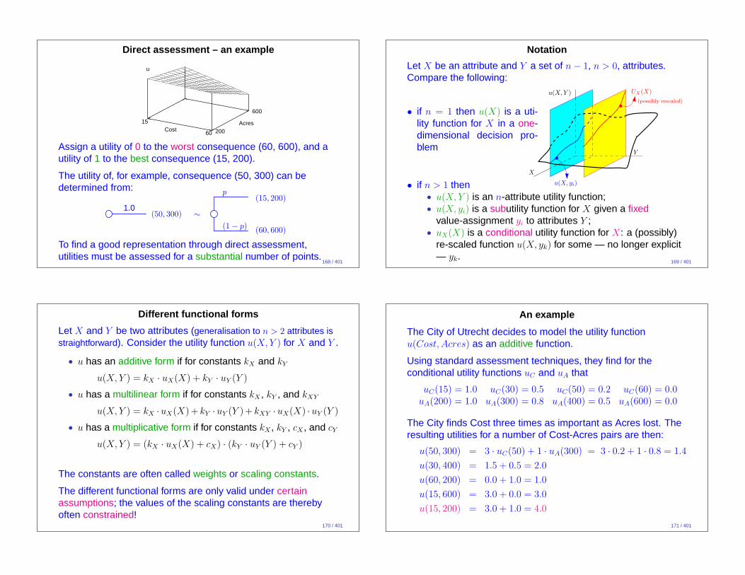
Direct assessment – an example

15

60Cost 200

600

Acres

u

Assign a utility of 0 to the worst consequence (60, 600), and autility of 1 to the best consequence (15, 200).

The utility of, for example, consequence (50, 300) can bedetermined from:

1.0(50, 300) ∼

p

(1− p)

(15, 200)

(60, 600)

To find a good representation through direct assessment,utilities must be assessed for a substantial number of points.

168 / 401

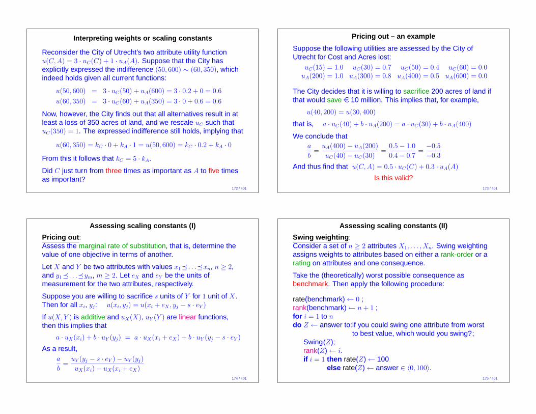
Notation

Let X be an attribute and Y a set of n− 1, n > 0, attributes.Compare the following:

• if n = 1 then u(X) is a uti-lity function for X in a one-dimensional decision pro-blem

X

Y

u(X, Y )

u(X, yi)

UX(X)

(possibly rescaled)

• if n > 1 then• u(X,Y ) is an n-attribute utility function;• u(X, yi) is a subutility function for X given a fixed

value-assignment yi to attributes Y ;• uX(X) is a conditional utility function for X: a (possibly)

re-scaled function u(X, yk) for some — no longer explicit— yk.

169 / 401

Different functional forms

Let X and Y be two attributes (generalisation to n > 2 attributes isstraightforward). Consider the utility function u(X,Y ) for X and Y .

• u has an additive form if for constants kX and kY

u(X,Y ) = kX · uX(X) + kY · uY (Y )

• u has a multilinear form if for constants kX , kY , and kXY

u(X,Y ) = kX ·uX(X)+ kY ·uY (Y )+ kXY ·uX(X) ·uY (Y )

• u has a multiplicative form if for constants kX , kY , cX , and cY

u(X,Y ) = (kX · uX(X) + cX) · (kY · uY (Y ) + cY )

The constants are often called weights or scaling constants.

The different functional forms are only valid under certainassumptions; the values of the scaling constants are therebyoften constrained!

170 / 401

An example

The City of Utrecht decides to model the utility functionu(Cost, Acres) as an additive function.

Using standard assessment techniques, they find for theconditional utility functions uC and uA that

uC(15) = 1.0 uC(30) = 0.5 uC(50) = 0.2 uC(60) = 0.0uA(200) = 1.0 uA(300) = 0.8 uA(400) = 0.5 uA(600) = 0.0

The City finds Cost three times as important as Acres lost. Theresulting utilities for a number of Cost-Acres pairs are then:

u(50, 300) = 3 · uC(50) + 1 · uA(300) = 3 · 0.2 + 1 · 0.8 = 1.4

u(30, 400) = 1.5 + 0.5 = 2.0

u(60, 200) = 0.0 + 1.0 = 1.0

u(15, 600) = 3.0 + 0.0 = 3.0

u(15, 200) = 3.0 + 1.0 = 4.0

171 / 401

Interpreting weights or scaling constants

Reconsider the City of Utrecht’s two attribute utility functionu(C,A) = 3 · uC(C) + 1 · uA(A). Suppose that the City hasexplicitly expressed the indifference (50, 600) ∼ (60, 350), whichindeed holds given all current functions:

u(50, 600) = 3 · uC(50) + uA(600) = 3 · 0.2 + 0 = 0.6

u(60, 350) = 3 · uC(60) + uA(350) = 3 · 0 + 0.6 = 0.6

Now, however, the City finds out that all alternatives result in atleast a loss of 350 acres of land, and we rescale uC such thatuC(350) = 1. The expressed indifference still holds, implying that

u(60, 350) = kC · 0 + kA · 1 = u(50, 600) = kC · 0.2 + kA · 0

From this it follows that kC = 5 · kA.

Did C just turn from three times as important as A to five timesas important?

172 / 401

Pricing out – an example

Suppose the following utilities are assessed by the City ofUtrecht for Cost and Acres lost:


The City decides that it is willing to sacrifice 200 acres of land ifthat would save e 10 million. This implies that, for example,

u(40, 200) = u(30, 400)

that is, a · uC(40) + b · uA(200) = a · uC(30) + b · uA(400)

We conclude thata

b=

uA(400)− uA(200)

uC(40)− uC(30)=

0.5− 1.0

0.4− 0.7=−0.5

−0.3

And thus find that u(C,A) = 0.5 · uC(C) + 0.3 · uA(A)

Is this valid?173 / 401

Assessing scaling constants (I)

Pricing out :Assess the marginal rate of substitution, that is, determine thevalue of one objective in terms of another.

Let X and Y be two attributes with values x1� . . .�xn, n ≥ 2,and y1� . . .�ym, m ≥ 2. Let eX and eY be the units ofmeasurement for the two attributes, respectively.

Suppose you are willing to sacrifice s units of Y for 1 unit of X.Then for all xi, yj: u(xi, yj) = u(xi + eX , yj − s · eY )

If u(X,Y ) is additive and uX(X), uY (Y ) are linear functions,then this implies that

a · uX(xi) + b · uY (yj) = a · uX(xi + eX) + b · uY (yj − s · eY )

As a result,a

b=

uY (yj − s · eY )− uY (yj)

uX(xi)− uX(xi + eX)

174 / 401

Assessing scaling constants (II)

Swing weighting :Consider a set of n ≥ 2 attributes X1, . . . , Xn. Swing weightingassigns weights to attributes based on either a rank-order or arating on attributes and one consequence.

Take the (theoretically) worst possible consequence asbenchmark. Then apply the following procedure:

rate(benchmark)← 0 ;rank(benchmark)← n + 1 ;for i = 1 to n

do Z ← answer to:if you could swing one attribute from worstto best value, which would you swing?;

Swing(Z);rank(Z)← i.if i = 1 then rate(Z)← 100

else rate(Z)← answer ∈ 〈0, 100〉.175 / 401

Swing weighting – cntd

Consider a set of n ≥ 2 attributes X1, . . . , Xn. Let rank(Xi) andrate(Xi) denote a ranking and a rating for attribute Xi,respectively.

The weight w(Xi) for attribute Xi can now be determined usingeither of the following two approaches:

• direct rating: w(Xi) =rate(Xi)

∑n

j=1rate(Xj)

• rank-sum weighing:

w(Xi) =reversed rank(Xi)

number of ranks=

n− rank(Xi) + 1

n + 1

176 / 401

Swing weighting – an example

Attribute consequenceto swing mill. e acres rank rate(benchmark) 60 600 2+1 0Cost 15 600 1 100Acres 60 200 2 30total: 3 130

direct rating :

w(C) =100

130= 0.77

w(A) =30

130= 0.23

rank-sum weighting :

w(C) =2− 1 + 1

3=

2

3

w(A) =2− 2 + 1

3=

1

3

177 / 401

Assessing scaling constants (III)

Lottery weights :Consider two attributes X and Y (the following extendsstraightforwardly to n > 2 attributes).

Let (x0, y0) denote the worst possible consequence, and(x+, y+) the best possible consequence.

The weight w(X) for attribute X equals p, where p is theindifference probability that follows from:

1.0(x+, y0) ∼

p

(1− p)

(x+, y+)

(x0, y0)

178 / 401

Lottery weights: an example

Assume once more that the City of Utrecht decides to model theutility function u(Cost, Acres) as an additive function:

u(C,A) = kC · uC(C) + kA · uA(A)

The weight kC is assessed from:

1.0(15, 600) ∼

kC

(1− kC)

(15, 200)

(60, 600)

The weight kA is assessed using:

1.0(60, 200) ∼

kA

(1− kA)

(15, 200)

(60, 600)

179 / 401

MAUT with n = 2 attributes:when can we use additive and multilinear forms?

180 / 401

Additive independence – the formal definition

Use of an additive utility function is justified given theassumption of additive independence [AI].

Two attributes X and Y are additive independent if preferencesfor lotteries over X × Y can be established by comparing thevalues one attribute at a time. More formally,

DEFINITION

Two attributes X and Y are additive independent if the pairedpreference comparison of any two lotteries, defined by two jointprobability distributions on X × Y , depends only on theirmarginal distributions.

181 / 401

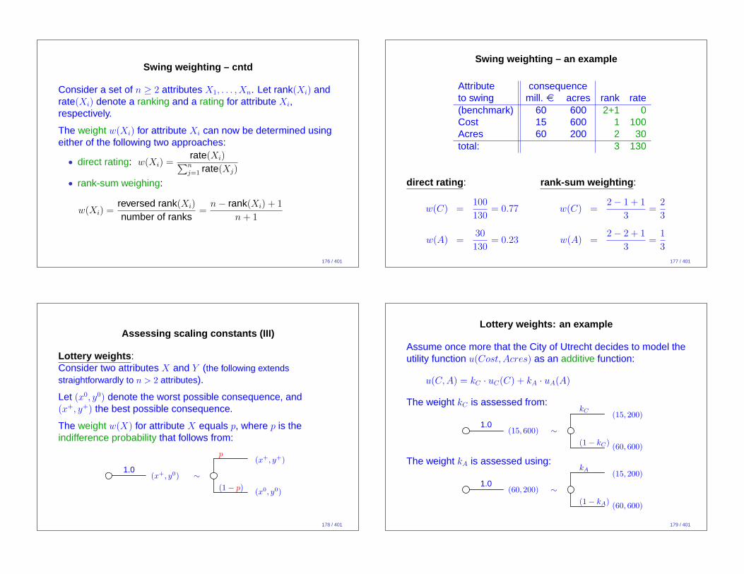
Interpreting additive independence

The ability to establish preferences for lotteries over X × Y bycomparing the values one attribute at a time entails thefollowing:

• the decisionmaker should be indifferent between

[p, (x1, y1); (1− p), (x2, y2)] and [p, (x1, y2); (1− p), (x2, y1)]

since both have the same probability of achieving x1 vs x2;

• the decisionmaker should also be indifferent between

[p, (x1, y1); (1− p), (x2, y2)] and [p, (x2, y1); (1− p), (x1, y2)]

since both have the same probability of achieving y1 vs y2;

• this can only hold if p = 1− p = 0.5

182 / 401

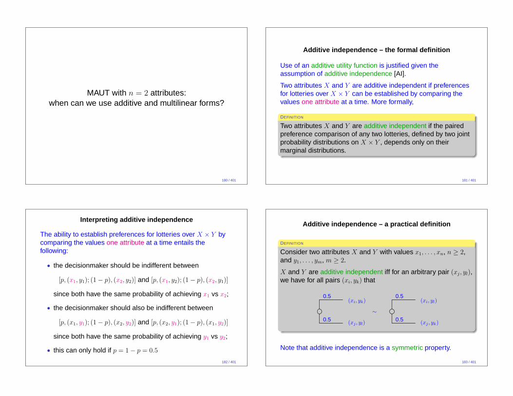
Additive independence – a practical definition

DEFINITION

Consider two attributes X and Y with values x1, . . . , xn, n ≥ 2,and y1, . . . , ym, m ≥ 2.

X and Y are additive independent iff for an arbitrary pair (xj, yl),we have for all pairs (xi, yk) that

0.5

0.5

(xi, yk)

(xj , yl)

∼

0.5

0.5

(xi, yl)

(xj , yk)

Note that additive independence is a symmetric property.

183 / 401

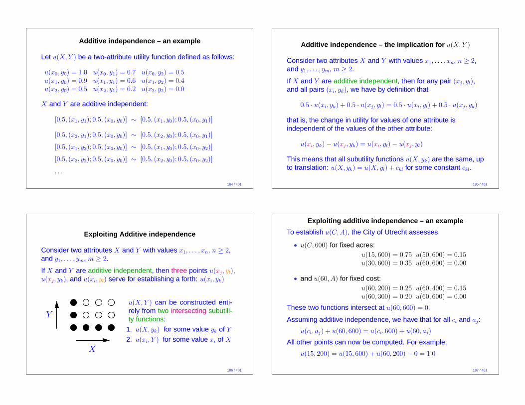
Additive independence – an example

Let u(X,Y ) be a two-attribute utility function defined as follows:

u(x0, y0) = 1.0 u(x0, y1) = 0.7 u(x0, y2) = 0.5u(x1, y0) = 0.9 u(x1, y1) = 0.6 u(x1, y2) = 0.4u(x2, y0) = 0.5 u(x2, y1) = 0.2 u(x2, y2) = 0.0

X and Y are additive independent:

[0.5, (x1, y1); 0.5, (x0, y0)] ∼ [0.5, (x1, y0); 0.5, (x0, y1)]

[0.5, (x2, y1); 0.5, (x0, y0)] ∼ [0.5, (x2, y0); 0.5, (x0, y1)]

[0.5, (x1, y2); 0.5, (x0, y0)] ∼ [0.5, (x1, y0); 0.5, (x0, y2)]

[0.5, (x2, y2); 0.5, (x0, y0)] ∼ [0.5, (x2, y0); 0.5, (x0, y2)]

. . .

184 / 401

Additive independence – the implication for u(X,Y )


If X and Y are additive independent, then for any pair (xj, yl),and all pairs (xi, yk), we have by definition that

0.5 · u(xi, yk) + 0.5 · u(xj, yl) = 0.5 · u(xi, yl) + 0.5 · u(xj, yk)

that is, the change in utility for values of one attribute isindependent of the values of the other attribute:

u(xi, yk)− u(xj, yk) = u(xi, yl)− u(xj, yl)

This means that all subutility functions u(X, yk) are the same, upto translation: u(X, yk) = u(X, yl) + ckl for some constant ckl.

185 / 401

Exploiting Additive independence


If X and Y are additive independent, then three points u(xj, yl),u(xj, yk), and u(xi, yl) serve for establishing a forth: u(xi, yk)

Y

X

u(X,Y ) can be constructed enti-rely from two intersecting subutili-ty functions:

1. u(X, yk) for some value yk of Y

2. u(xi, Y ) for some value xi of X

186 / 401

Exploiting additive independence – an example

To establish u(C,A), the City of Utrecht assesses

• u(C, 600) for fixed acres:u(15, 600) = 0.75 u(50, 600) = 0.15u(30, 600) = 0.35 u(60, 600) = 0.00

• and u(60, A) for fixed cost:u(60, 200) = 0.25 u(60, 400) = 0.15u(60, 300) = 0.20 u(60, 600) = 0.00

These two functions intersect at u(60, 600) = 0.

Assuming additive independence, we have that for all ci and aj:

u(ci, aj) + u(60, 600) = u(ci, 600) + u(60, aj)

All other points can now be computed. For example,

u(15, 200) = u(15, 600) + u(60, 200)− 0 = 1.0

187 / 401

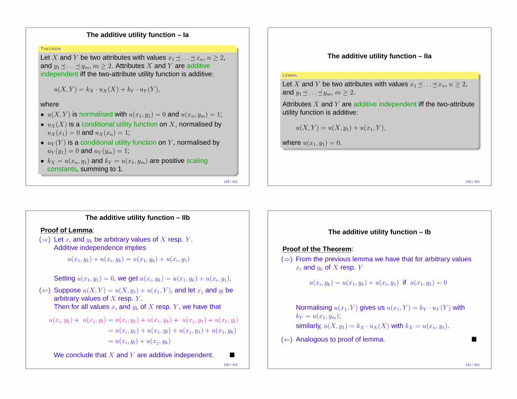
The additive utility function – Ia

THEOREM

Let X and Y be two attributes with values x1� . . .�xn, n ≥ 2,and y1� . . .�ym, m ≥ 2. Attributes X and Y are additiveindependent iff the two-attribute utility function is additive:

u(X,Y ) = kX · uX(X) + kY · uY (Y ),

where

• u(X,Y ) is normalised with u(x1, y1) = 0 and u(xn, ym) = 1;

• uX(X) is a conditional utility function on X, normalised byuX(x1) = 0 and uX(xn) = 1;

• uY (Y ) is a conditional utility function on Y , normalised byuY (y1) = 0 and uY (ym) = 1;

• kX = u(xn, y1) and kY = u(x1, ym) are positive scalingconstants, summing to 1.

188 / 401

The additive utility function – IIa

LEMMA

Let X and Y be two attributes with values x1� . . .�xn, n ≥ 2,and y1� . . .�ym, m ≥ 2.

Attributes X and Y are additive independent iff the two-attributeutility function is additive:

u(X,Y ) = u(X, y1) + u(x1, Y ),

where u(x1, y1) = 0.

189 / 401

The additive utility function – IIb

Proof of Lemma :(⇒) Let xi and yk be arbitrary values of X resp. Y .

Additive independence implies

u(x1, y1) + u(xi, yk) = u(x1, yk) + u(xi, y1)

Setting u(x1, y1) = 0, we get u(xi, yk) = u(x1, yk) + u(xi, y1).

(⇐) Suppose u(X,Y ) = u(X, y1) + u(x1, Y ), and let xj and yl bearbitrary values of X resp. Y .Then for all values xi and yk of X resp. Y , we have that

u(xi, yk) + u(xj, yl) = u(xi, y1) + u(x1, yk) + u(xj, y1) + u(x1, yl)

= u(xi, y1) + u(x1, yl) + u(xj, y1) + u(x1, yk)

= u(xi, yl) + u(xj, yk)

We conclude that X and Y are additive independent. �

190 / 401

The additive utility function – Ib

Proof of the Theorem :

(⇒) From the previous lemma we have that for arbitrary valuesxi and yk of X resp. Y

u(xi, yk) = u(x1, yk) + u(xi, y1) if u(x1, y1) = 0

Normalising u(x1, Y ) gives us u(x1, Y ) = kY · uY (Y ) withkY = u(x1, ym);

similarly, u(X, y1) = kX · uX(X) with kX = u(xn, y1).

(⇐) Analogous to proof of lemma. �

191 / 401

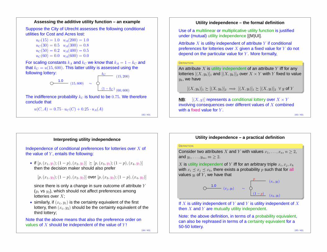
Assessing the additive utility function – an example

Suppose the City of Utrecht assesses the following conditionalutilities for Cost and Acres lost:

uC(15) = 1.0 uA(200) = 1.0uC(30) = 0.5 uA(300) = 0.8uC(50) = 0.2 uA(400) = 0.5uC(60) = 0.0 uA(600) = 0.0

For scaling constants kA and kC we know that kA = 1− kC andthat kC = u(15, 600). This latter utility is assessed using thefollowing lottery:

1.0(15, 600) ∼

kC

(1− kC)

(15, 200)

(60, 600)

The indifference probability kC is found to be 0.75. We thereforeconclude that

u(C,A) = 0.75 · uC(C) + 0.25 · uA(A)192 / 401

Utility independence – the formal definition

Use of a multilinear or multiplicative utility function is justifiedunder (mutual) utility independence [(M)UI].

Attribute X is utility independent of attribute Y if conditionalpreferences for lotteries over X given a fixed value for Y do notdepend on the particular value for Y . More formally,

DEFINITION

An attribute X is utility independent of an attribute Y iff for anylotteries [(X, yk)]1 and [(X, yk)]2 over X × Y with Y fixed to valueyk, we have

[(X, yk)]1 � [(X, yk)]2 =⇒ [(X, yl)]1 � [(X, yl)]2 ∀ y of Y

NB: [(X, y)] represents a conditional lottery over X × Y

involving consequences over different values of X combinedwith a fixed value for Y .

193 / 401

Interpreting utility independence

Independence of conditional preferences for lotteries over X ofthe value of Y , entails the following:

• if [p, (x1, y1); (1− p), (x2, y1)] � [p, (x3, y1); (1− p), (x4, y1)]then the decision maker should also prefer

[p, (x1, y2); (1− p), (x2, y2)] over [p, (x3, y2); (1− p), (x4, y2)]

since there is only a change in sure outcome of attribute Y

(y1 vs y2), which should not affect preferences amonglotteries over X;

• similarly, if (xC, y1) is the certainty equivalent of the firstlottery, then (xC, y2) should be the certainty equivalent of thethird lottery;

Note that the above means that also the preference order onvalues of X should be independent of the value of Y !

194 / 401

Utility independence – a practical definition

DEFINITION


X is utility independent of Y iff for an arbitrary triple xi, xj, xk

with xi � xj � xk, there exists a probability p such that for allvalues yl of Y , we have that

1.0(xj , yl) ∼

p

(1− p)

(xi, yl)

(xk, yl)

If X is utility independent of Y and Y is utility independent of X

then X and Y are mutually utility independent.

Note: the above definition, in terms of a probability equivalent,can also be rephrased in terms of a certainty equivalent for a50-50 lottery.

195 / 401

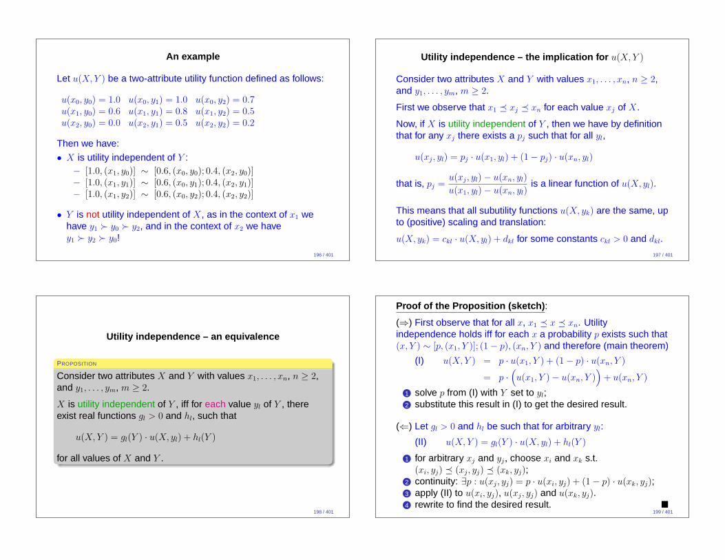
An example

Let u(X,Y ) be a two-attribute utility function defined as follows:


Then we have:

• X is utility independent of Y :− [1.0, (x1, y0)] ∼ [0.6, (x0, y0); 0.4, (x2, y0)]− [1.0, (x1, y1)] ∼ [0.6, (x0, y1); 0.4, (x2, y1)]− [1.0, (x1, y2)] ∼ [0.6, (x0, y2); 0.4, (x2, y2)]

• Y is not utility independent of X, as in the context of x1 wehave y1 ≻ y0 ≻ y2, and in the context of x2 we havey1 ≻ y2 ≻ y0!

196 / 401

Utility independence – the implication for u(X,Y )


First we observe that x1 � xj � xn for each value xj of X.

Now, if X is utility independent of Y , then we have by definitionthat for any xj there exists a pj such that for all yl,

u(xj, yl) = pj · u(x1, yl) + (1− pj) · u(xn, yl)

that is, pj =u(xj, yl)− u(xn, yl)

u(x1, yl)− u(xn, yl)is a linear function of u(X, yl).

This means that all subutility functions u(X, yk) are the same, upto (positive) scaling and translation:

u(X, yk) = ckl · u(X, yl) + dkl for some constants ckl > 0 and dkl.

197 / 401

Utility independence – an equivalence

PROPOSITION


X is utility independent of Y , iff for each value yl of Y , thereexist real functions gl > 0 and hl, such that

u(X,Y ) = gl(Y ) · u(X, yl) + hl(Y )

for all values of X and Y .

198 / 401

Proof of the Proposition (sketch) :

(⇒) First observe that for all x, x1 � x � xn. Utilityindependence holds iff for each x a probability p exists such that(x, Y ) ∼ [p, (x1, Y )]; (1− p), (xn, Y ) and therefore (main theorem)

(I) u(X,Y ) = p · u(x1, Y ) + (1− p) · u(xn, Y )

= p ·(

u(x1, Y )− u(xn, Y ))

+ u(xn, Y )

1 solve p from (I) with Y set to yl;2 substitute this result in (I) to get the desired result.

(⇐) Let gl > 0 and hl be such that for arbitrary yl:

(II) u(X,Y ) = gl(Y ) · u(X, yl) + hl(Y )

1 for arbitrary xj and yj, choose xi and xk s.t.(xi, yj) � (xj, yj) � (xk, yj);

2 continuity: ∃p : u(xj, yj) = p · u(xi, yj) + (1− p) · u(xk, yj);3 apply (II) to u(xi, yj), u(xj, yj) and u(xk, yj).4 rewrite to find the desired result. �

199 / 401

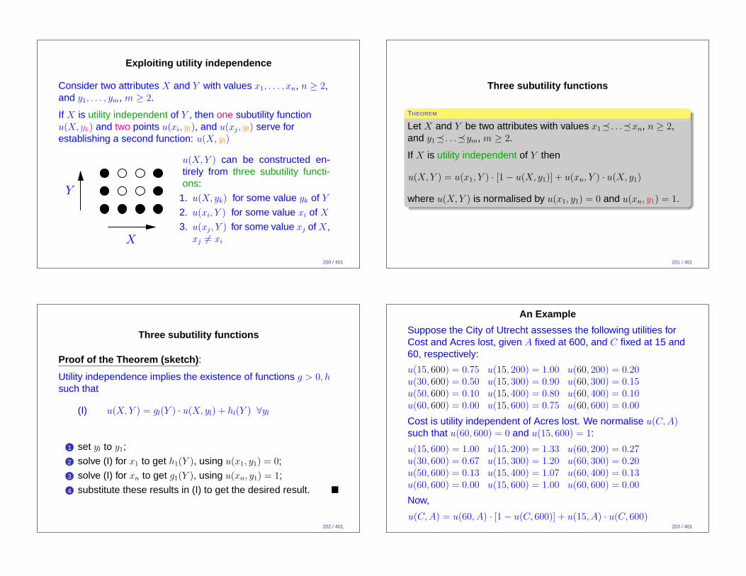
Exploiting utility independence


If X is utility independent of Y , then one subutility functionu(X, yk) and two points u(xi, yl), and u(xj, yl) serve forestablishing a second function: u(X, yl)

Y

X

u(X,Y ) can be constructed en-tirely from three subutility functi-ons:



3. u(xj, Y ) for some value xj of X,xj 6= xi

200 / 401

Three subutility functions

THEOREM


If X is utility independent of Y then

u(X,Y ) = u(x1, Y ) · [1− u(X, y1)] + u(xn, Y ) · u(X, y1)

where u(X,Y ) is normalised by u(x1, y1) = 0 and u(xn, y1) = 1.

201 / 401

Three subutility functions

Proof of the Theorem (sketch) :

Utility independence implies the existence of functions g > 0, hsuch that

(I) u(X,Y ) = gl(Y ) · u(X, yl) + hl(Y ) ∀yl

1 set yl to y1;

2 solve (I) for x1 to get h1(Y ), using u(x1, y1) = 0;

3 solve (I) for xn to get g1(Y ), using u(xn, y1) = 1;

4 substitute these results in (I) to get the desired result. �

202 / 401

An Example

Suppose the City of Utrecht assesses the following utilities forCost and Acres lost, given A fixed at 600, and C fixed at 15 and60, respectively:

u(15, 600) = 0.75 u(15, 200) = 1.00 u(60, 200) = 0.20u(30, 600) = 0.50 u(15, 300) = 0.90 u(60, 300) = 0.15u(50, 600) = 0.10 u(15, 400) = 0.80 u(60, 400) = 0.10u(60, 600) = 0.00 u(15, 600) = 0.75 u(60, 600) = 0.00

Cost is utility independent of Acres lost. We normalise u(C,A)such that u(60, 600) = 0 and u(15, 600) = 1:

u(15, 600) = 1.00 u(15, 200) = 1.33 u(60, 200) = 0.27u(30, 600) = 0.67 u(15, 300) = 1.20 u(60, 300) = 0.20u(50, 600) = 0.13 u(15, 400) = 1.07 u(60, 400) = 0.13u(60, 600) = 0.00 u(15, 600) = 1.00 u(60, 600) = 0.00

Now,

u(C,A) = u(60, A) · [1− u(C, 600)] + u(15, A) · u(C, 600)203 / 401

The additive utility function — IIIa

COROLLARY


If X is utility independent of Y , then

the two-attribute utility function is additive iff

[0.5, (x1, y1); 0.5, (xn, Y )] ∼ [0.5, (x1, Y ); 0.5, (xn, y1)]

Under the above conditions, we have that

u(X,Y ) = u(x1, Y ) + u(X, y1)

where u(x1, y1) = 0 and u(xn, y1) = 1.204 / 401

The additive utility function — IIIb

Proof of the Corollary :

Utility independence implies that

u(X,Y ) = u(x1, Y ) [1− u(X, y1)] + u(xn, Y ) · u(X, y1)

with u(x1, y1) = 0 and u(xn, y1) = 1.

The lottery equivalence translates into

0 + u(xn, Y ) = 1 + u(x1, Y )

Substitute u(xn, Y ) with 1 + u(x1, Y ) in the above results in

u(X,Y ) = u(x1, Y ) + u(X, y1)

with u(x1, y1) = 0 and u(xn, y1) = 1 �

205 / 401

The multilinear utility function — Ia

COROLLARY


If X is utility independent of Y , then

the two-attribute utility function is multilinear iff

u(xn, Y ) = 1 + b · u(x1, Y )

for some constant b > 0.


u(X,Y ) = u(x1, Y ) + u(X, y1) + (b− 1) · u(x1, Y ) · u(X, y1)

where u(x1, y1) = 0 and u(xn, y1) = 1.206 / 401

The multilinear utility function — Ia

Proof of the Corollary :

Utility independence implies that


with u(x1, y1) = 0 and u(xn, y1) = 1.

Substitute u(xn, Y ) with 1 + b · u(x1, Y ) in the above results in

u(X,Y ) = u(x1, Y ) + u(X, y1) + (b− 1) · u(x1, Y ) · u(X, y1)

with u(x1, y1) = 0 and u(xn, y1) = 1. �

207 / 401

Exploiting mutual utility independence


If X and Y are mutually utility independent, then u(X,Y ) can beconstructed from two subutility functions and one point:



3. u(xj, yl) for some values xj 6= xi of X, and yl 6= yk of Y

if X is utility independent ofY , but Y is utility dependentof X:

Y

X

if X and Y are mutually utilityindependent:

Y

X208 / 401

Exploiting mutual utility independence – example

Suppose the utilities, given fixed A = 60 resp. C = 600,assessed by the City of Utrecht are:

u(15, 600) = 0.75 u(30, 600) = 0.35 u(50, 600) = 0.15 u(60, 600)u(60, 200) = 0.25 u(60, 300) = 0.20 u(60, 400) = 0.15 = 0.00

In addition, the utility u(30, 300) = 0.30 is assessed.

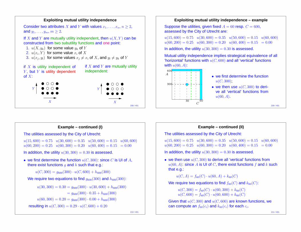
Mutual utility independence implies strategical equivalence of all’horizontal’ functions with u(C, 600) and all ’vertical’ functionswith u(60, A):

C

A

30 60

300

600

• we first determine the functionu(C, 300);

• we then use u(C, 300) to deri-ve all ’vertical’ functions fromu(60, A).

209 / 401

Example – continued (I)

The utilities assessed by the City of Utrecht:

u(15, 600) = 0.75 u(30, 600) = 0.35 u(50, 600) = 0.15 u(60, 600)u(60, 200) = 0.25 u(60, 300) = 0.20 u(60, 400) = 0.15 = 0.00


• we first determine the function u(C, 300): since C is UI of A,there exist functions g and h such that e.g.:

u(C, 300) = g600(300) · u(C, 600) + h600(300)

We require two equations to find g600(300) and h600(300):

u(30, 300) = 0.30 = g600(300) · u(30, 600) + h600(300)

= g600(300) · 0.35 + h600(300)

u(60, 300) = 0.20 = g600(300) · 0.00 + h600(300)

resulting in u(C, 300) = 0.29 · u(C, 600) + 0.20

210 / 401

Example – continued (II)

The utilities assessed by the City of Utrecht:

u(15, 600) = 0.75 u(30, 600) = 0.35 u(50, 600) = 0.15 u(60, 600)u(60, 200) = 0.25 u(60, 300) = 0.20 u(60, 400) = 0.15 = 0.00


• we then use u(C, 300) to derive all ’vertical’ functions fromu(60, A): since A is UI of C, there exist functions f and k suchthat e.g.:

u(C,A) = f60(C) · u(60, A) + k60(C)

We require two equations to find f60(C) and k60(C):

u(C, 300) = f60(C) · u(60, 300) + k60(C)u(C, 600) = f60(C) · u(60, 600) + k60(C)

Given that u(C, 300) and u(C, 600) are known functions, wecan compute an f60(ci) and k60(ci) for each ci.

211 / 401

The multilinear utility function — IIa

THEOREM

Let X and Y be two attributes with values x1� . . .�xn, n ≥ 2,and y1� . . .�ym, m ≥ 2. If X and Y are mutually utilityindependent then the two-attribute utility function is multilinear:

u(X,Y ) = kX · uX(X) + kY · uY (Y ) + kXY · uX(X) · uY (Y )

where

• u(X,Y ) is normalised by u(x1, y1) = 0 and u(xn, ym) = 1;

• uX(X) is a conditional utility function on X, normalised byuX(x1) = 0 and uX(xn) = 1;

• uY (Y ) is a conditional utility function on Y , normalised byuY (y1) = 0 and uY (ym) = 1;

• kX = u(xn, y1) > 0, kY = u(x1, ym) > 0, kXY = 1− kX − kY arescaling constants.

212 / 401

The multilinear utility function — IIIa

LEMMA


If X and Y are mutually utility independent then the two-attributeutility function is multilinear:

u(X,Y ) = u(X, y1) + u(x1, Y ) + k · u(X, y1) · u(x1, Y )

where

• u(x1, y1) = 0, u(xn, y1) > 0 and u(x1, ym) > 0;

• k =u(xn, ym)− u(xn, y1)− u(x1, ym)

u(xn, y1) · u(x1, ym)is a scaling constant.

213 / 401

The multilinear utility function — IIIb

Proof of Lemma: (sketch) :

Mutual utility independence implies the existence of functionsf > 0, g > 0, h, and k such that for arbitrary xl and yl

(I) u(X,Y ) = gl(Y ) · u(X, yl) + hl(Y ) and

(II) u(X,Y ) = fl(X) · u(xl, Y ) + kl(X)

1 set yl to y1 and xl to x1

2 solve (I) for x1 to get h1(Y ) and for xn to get g1(Y )

3 solve (II) for y1 to get k1(X) and for ym to get f1(X)

4 substitute these results in (I) and (II)→ (I*) and (II*)

5 now solve (II*) for xn and fill in this result in (I*) to get thedesired result. �

214 / 401

The multilinear utility function — IIb

Proof of the Theorem :From the previous lemma we have that for arbitrary values xi

and yj of X resp. Y , we have

u(xi, yj) = u(xi, y1) + u(x1, yj) + k · u(xi, y1) · u(x1, yj)

if u(x1, y1) = 0, u(xn, y1) > 0 and u(x1, ym) > 0;

Normalising u(x1, Y ) gives us u(x1, Y ) = kY · uY (Y ) withkY = u(x1, ym).

Similarly, u(X, y1) = kX · uX(X) with kX = u(xn, y1).

Finally, define kXY = k · kX · kY . �

215 / 401

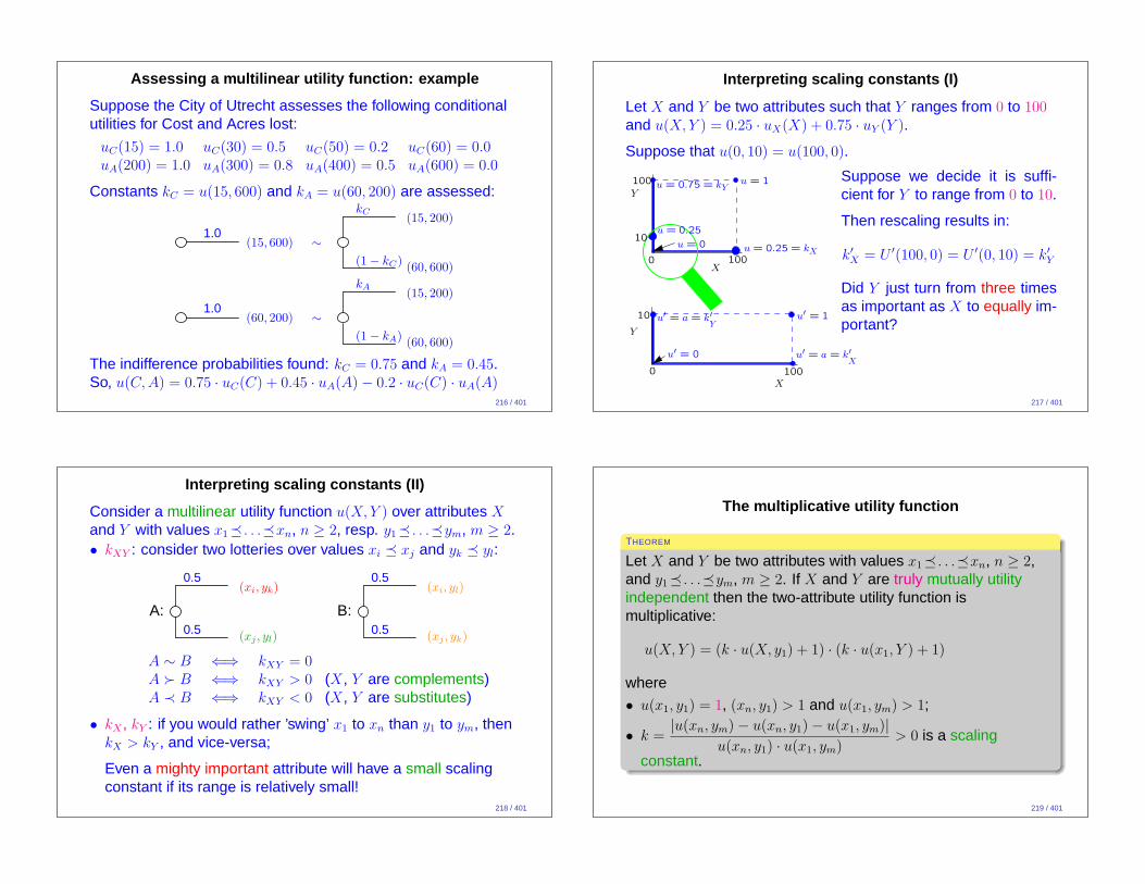
Assessing a multilinear utility function: example



Constants kC = u(15, 600) and kA = u(60, 200) are assessed:

1.0(15, 600) ∼

kC

(1− kC)

(15, 200)

(60, 600)

1.0(60, 200) ∼

kA

(1− kA)

(15, 200)

(60, 600)

The indifference probabilities found: kC = 0.75 and kA = 0.45.So, u(C,A) = 0.75 · uC(C) + 0.45 · uA(A)− 0.2 · uC(C) · uA(A)

216 / 401

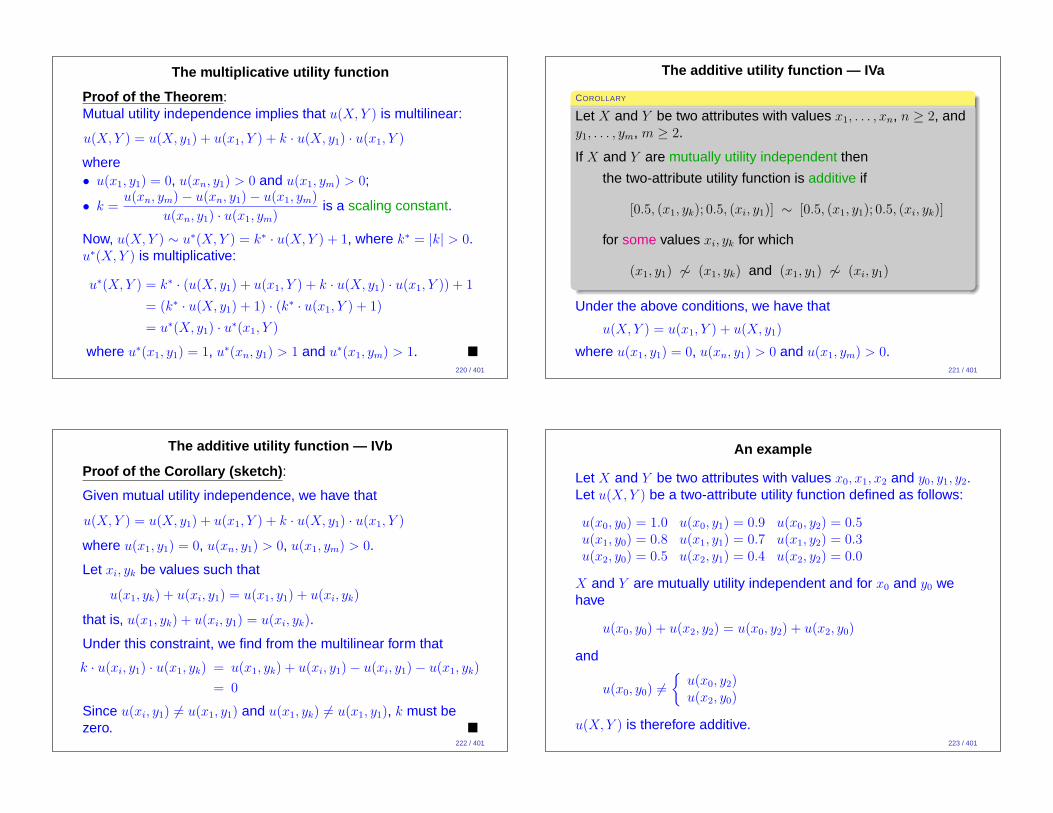
Interpreting scaling constants (I)

Let X and Y be two attributes such that Y ranges from 0 to 100and u(X,Y ) = 0.25 · uX(X) + 0.75 · uY (Y ).

Suppose that u(0, 10) = u(100, 0).

0

100

100

0

10

100

X

Y

Y

X

10

u = 1

u′ = 1

u = 0.25 = kX

u = 0.25

u = 0

u′ = 0

u = 0.75 = kY

u′ = a = k′X

u′ = a = k′Y

Suppose we decide it is suffi-cient for Y to range from 0 to 10.

Then rescaling results in:

k′

X = U ′(100, 0) = U ′(0, 10) = k′

Y

Did Y just turn from three timesas important as X to equally im-portant?

217 / 401

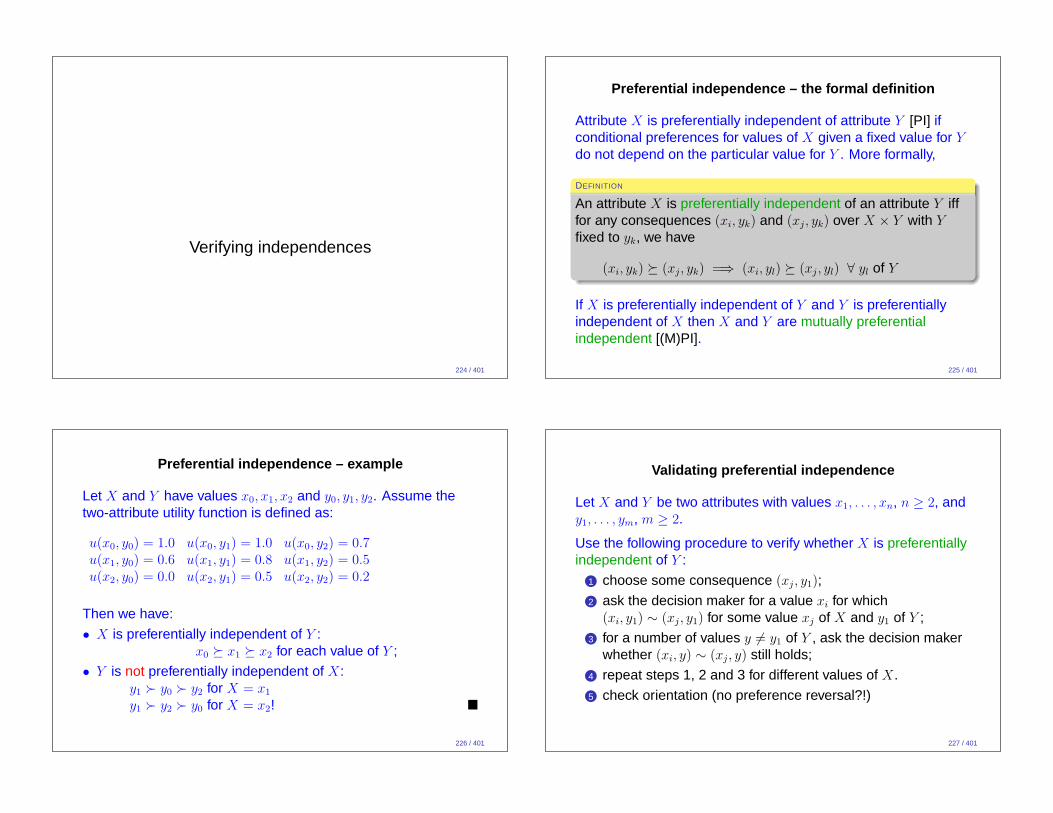
Interpreting scaling constants (II)

Consider a multilinear utility function u(X,Y ) over attributes X

and Y with values x1� . . .�xn, n ≥ 2, resp. y1� . . .�ym, m ≥ 2.• kXY : consider two lotteries over values xi � xj and yk � yl:

0.5

0.5

(xi, yk)

(xj , yl)

A:

0.5

0.5

(xi, yl)

(xj , yk)

B:

A ∼ B ⇐⇒ kXY = 0A ≻ B ⇐⇒ kXY > 0 (X, Y are complements)A ≺ B ⇐⇒ kXY < 0 (X, Y are substitutes)

• kX , kY : if you would rather ’swing’ x1 to xn than y1 to ym, thenkX > kY , and vice-versa;

Even a mighty important attribute will have a small scalingconstant if its range is relatively small!

218 / 401

The multiplicative utility function

THEOREM

Let X and Y be two attributes with values x1� . . .�xn, n ≥ 2,and y1� . . .�ym, m ≥ 2. If X and Y are truly mutually utilityindependent then the two-attribute utility function ismultiplicative:

u(X,Y ) = (k · u(X, y1) + 1) · (k · u(x1, Y ) + 1)

where

• u(x1, y1) = 1, (xn, y1) > 1 and u(x1, ym) > 1;

• k =|u(xn, ym)− u(xn, y1)− u(x1, ym)|

u(xn, y1) · u(x1, ym)> 0 is a scaling

constant.

219 / 401

The multiplicative utility function

Proof of the Theorem :Mutual utility independence implies that u(X,Y ) is multilinear:


where• u(x1, y1) = 0, u(xn, y1) > 0 and u(x1, ym) > 0;

• k =u(xn, ym)− u(xn, y1)− u(x1, ym)

u(xn, y1) · u(x1, ym)is a scaling constant.

Now, u(X,Y ) ∼ u∗(X,Y ) = k∗ · u(X,Y ) + 1, where k∗ = |k| > 0.u∗(X,Y ) is multiplicative:

u∗(X,Y ) = k∗ · (u(X, y1) + u(x1, Y ) + k · u(X, y1) · u(x1, Y )) + 1

= (k∗ · u(X, y1) + 1) · (k∗ · u(x1, Y ) + 1)

= u∗(X, y1) · u∗(x1, Y )

where u∗(x1, y1) = 1, u∗(xn, y1) > 1 and u∗(x1, ym) > 1. �

220 / 401

The additive utility function — IVa

COROLLARY

Let X and Y be two attributes with values x1, . . . , xn, n ≥ 2, andy1, . . . , ym, m ≥ 2.

If X and Y are mutually utility independent then

the two-attribute utility function is additive if

[0.5, (x1, yk); 0.5, (xi, y1)] ∼ [0.5, (x1, y1); 0.5, (xi, yk)]

for some values xi, yk for which

(x1, y1) 6∼ (x1, yk) and (x1, y1) 6∼ (xi, y1)


u(X,Y ) = u(x1, Y ) + u(X, y1)

where u(x1, y1) = 0, u(xn, y1) > 0 and u(x1, ym) > 0.221 / 401

The additive utility function — IVb

Proof of the Corollary (sketch) :

Given mutual utility independence, we have that


where u(x1, y1) = 0, u(xn, y1) > 0, u(x1, ym) > 0.

Let xi, yk be values such that

u(x1, yk) + u(xi, y1) = u(x1, y1) + u(xi, yk)

that is, u(x1, yk) + u(xi, y1) = u(xi, yk).

Under this constraint, we find from the multilinear form that

k · u(xi, y1) · u(x1, yk) = u(x1, yk) + u(xi, y1)− u(xi, y1)− u(x1, yk)

= 0

Since u(xi, y1) 6= u(x1, y1) and u(x1, yk) 6= u(x1, y1), k must bezero. �

222 / 401

An example

Let X and Y be two attributes with values x0, x1, x2 and y0, y1, y2.Let u(X,Y ) be a two-attribute utility function defined as follows:


X and Y are mutually utility independent and for x0 and y0 wehave

u(x0, y0) + u(x2, y2) = u(x0, y2) + u(x2, y0)

and

u(x0, y0) 6=

{

u(x0, y2)u(x2, y0)

u(X,Y ) is therefore additive.223 / 401

Verifying independences

224 / 401

Preferential independence – the formal definition

Attribute X is preferentially independent of attribute Y [PI] ifconditional preferences for values of X given a fixed value for Y

do not depend on the particular value for Y . More formally,

DEFINITION

An attribute X is preferentially independent of an attribute Y ifffor any consequences (xi, yk) and (xj, yk) over X × Y with Y

fixed to yk, we have

(xi, yk) � (xj, yk) =⇒ (xi, yl) � (xj, yl) ∀ yl of Y

If X is preferentially independent of Y and Y is preferentiallyindependent of X then X and Y are mutually preferentialindependent [(M)PI].

225 / 401

Preferential independence – example

Let X and Y have values x0, x1, x2 and y0, y1, y2. Assume thetwo-attribute utility function is defined as:


Then we have:

• X is preferentially independent of Y :x0 � x1 � x2 for each value of Y ;

• Y is not preferentially independent of X:y1 ≻ y0 ≻ y2 for X = x1

y1 ≻ y2 ≻ y0 for X = x2! �

226 / 401

Validating preferential independence

Let X and Y be two attributes with values x1, . . . , xn, n ≥ 2, andy1, . . . , ym, m ≥ 2.

Use the following procedure to verify whether X is preferentiallyindependent of Y :

1 choose some consequence (xj, y1);

2 ask the decision maker for a value xi for which(xi, y1) ∼ (xj, y1) for some value xj of X and y1 of Y ;

3 for a number of values y 6= y1 of Y , ask the decision makerwhether (xi, y) ∼ (xj, y) still holds;

4 repeat steps 1, 2 and 3 for different values of X.

5 check orientation (no preference reversal?!)

227 / 401

UI implies PI

PROPOSITION


If X is utility independent of Y then X is preferentiallyindependent of Y .

Proof : Consider xi, xj and yk such that (xi, yk) � u(xj, yk),that is, u(xi, yk)− u(xj, yk) ≥ 0.

UI now implies the existence of functions g > 0 and h such thatfor arbitrary yl:

u(xi, yk) = gl(yk) · u(xi, yl) + hl(yk) and

u(xj, yk) = gl(yk) · u(xj, yl) + hl(yk)

From gl(yk) > 0, we now have u(xi, yl)− u(xj, yl) ≥ 0 forarbitrary yl. �

228 / 401

PI implies UI ?

If X is preferentially independent of Y then X not necessarilyutility independent of Y .

Counter example :

Consider the following utility function:

u(x0, y0) = 1.0 u(x1, y0) = 0.8 u(x2, y0) = 0.3u(x0, y1) = 0.5 u(x1, y1) = 0.1 u(x2, y1) = 0.1

• X PI Y since ∀yi: x0 � x1 � x2;• we have no X UI Y :

(x1, y) ∼ [p, (x0, y); (1− p), (x2, y)]

holds for p ≈ 0.71 if y ≡ y0, and for p = 0, if y ≡ y1.229 / 401

Validating utility independence

If X PI Y , then X is also utility independent of Y if in thefollowing procedure xC is equivalent for all values of Y :

1 choose a lottery [0.5, P ; 0.5, Q] where P = (x1, y) andQ = (xn, y) for some value y of Y and values x1 and xn of X;

2 ask the decision maker whether or not he prefers the lottery[0.5, P ; 0.5, Q] to a consequence (xi, y) for some xi,x1 � xi � xn;

3 repeat step 2 until youconverge to the certaintyequivalent (xC , y) of thelottery;

4 repeat steps 1 – 3 fordifferent values of Y .

Repeat the procedure for dif-ferent pairs of values for X.

x1 xn

X

Y

ym

y1

Q

Q′′

Q′

P ′

P ′′

P xC

xC

xC

230 / 401

AI implies (M)UI

PROPOSITION


If X and Y are additive independent then X and Y are mutuallyutility independent

Proof (sketch) : We prove X UI Y ; Y UI X is analogous.

AI implies u(X, yk) = u(X, y1) + u(x1, yk) for arbitrary yk, whereu(x1, yk) is constant w.r.t the value of X.

Continuity implies, for arbitrary xi, xj and xk with(xi, y1) � (xj, y1) � (xk, y1), that ∃p such that(I) u(xj, y1) = p · u(xi, y1) + (1− p) · u(xk, y1).

Substitution of each u(X, y1) in (I) with u(X, yk)− u(x1, yk) givesu(xj, yk) = p · u(xi, yk) + (1− p) · u(xk, yk) for arbitrary yk. �

231 / 401

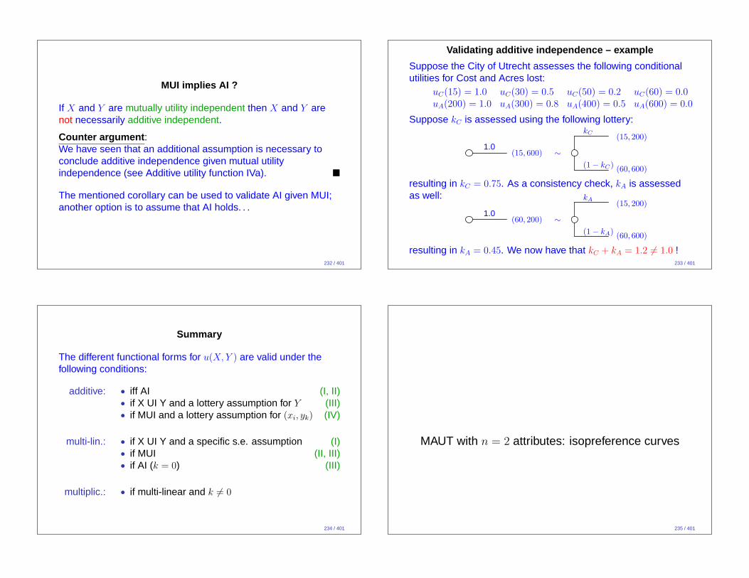
MUI implies AI ?

If X and Y are mutually utility independent then X and Y arenot necessarily additive independent.

Counter argument :We have seen that an additional assumption is necessary toconclude additive independence given mutual utilityindependence (see Additive utility function IVa). �

The mentioned corollary can be used to validate AI given MUI;another option is to assume that AI holds. . .

232 / 401

Validating additive independence – example



Suppose kC is assessed using the following lottery:

1.0(15, 600) ∼

kC

(1− kC)

(15, 200)

(60, 600)

resulting in kC = 0.75. As a consistency check, kA is assessedas well:

1.0(60, 200) ∼

kA

(1− kA)

(15, 200)

(60, 600)

resulting in kA = 0.45. We now have that kC + kA = 1.2 6= 1.0 !233 / 401

Summary

The different functional forms for u(X,Y ) are valid under thefollowing conditions:

additive: • iff AI (I, II)• if X UI Y and a lottery assumption for Y (III)• if MUI and a lottery assumption for (xi, yk) (IV)

multi-lin.: • if X UI Y and a specific s.e. assumption (I)• if MUI (II, III)• if AI (k = 0) (III)

multiplic.: • if multi-linear and k 6= 0

234 / 401

MAUT with n = 2 attributes: isopreference curves

235 / 401

Utility functions with one utility independent attribute

Let X and Y be two attributes. Suppose that X is utilityindependent of Y , but the reverse does not hold.

Recall that the two-attribute utility function can be specifiedusing three subutility functions:


where u(x1, y1) = 0 and u(xn, y1) = 1.

Other options are:

replacing one or two subutility functions with one or two,respectively, isopreference curves.

236 / 401

Isopreference curves – definition

An isopreference curve describes a set of consequences thatare equally desirable to the decision maker.

DEFINITION

Consider two (sets of) attributes X and Y and a partial functioni : X → Y such that for arbitrary values xi 6= xk of X and yj, yl ofY , we have that

i(xi) = yj and i(xk) = yl ⇐⇒ (xi, yj) ∼ (xk, yl)

An isopreference curve is an interpolant~ıY (X) of i(X).

Note that for any two points (xi, yj) and (xk, yl) on theisopreference curve, we thus have that

u(xi, yj) = u(xk, yl) = c for some constant c.

As a result, u(X,~ıY (X)) = c is a constant subutility function,defined on all values of X. 237 / 401

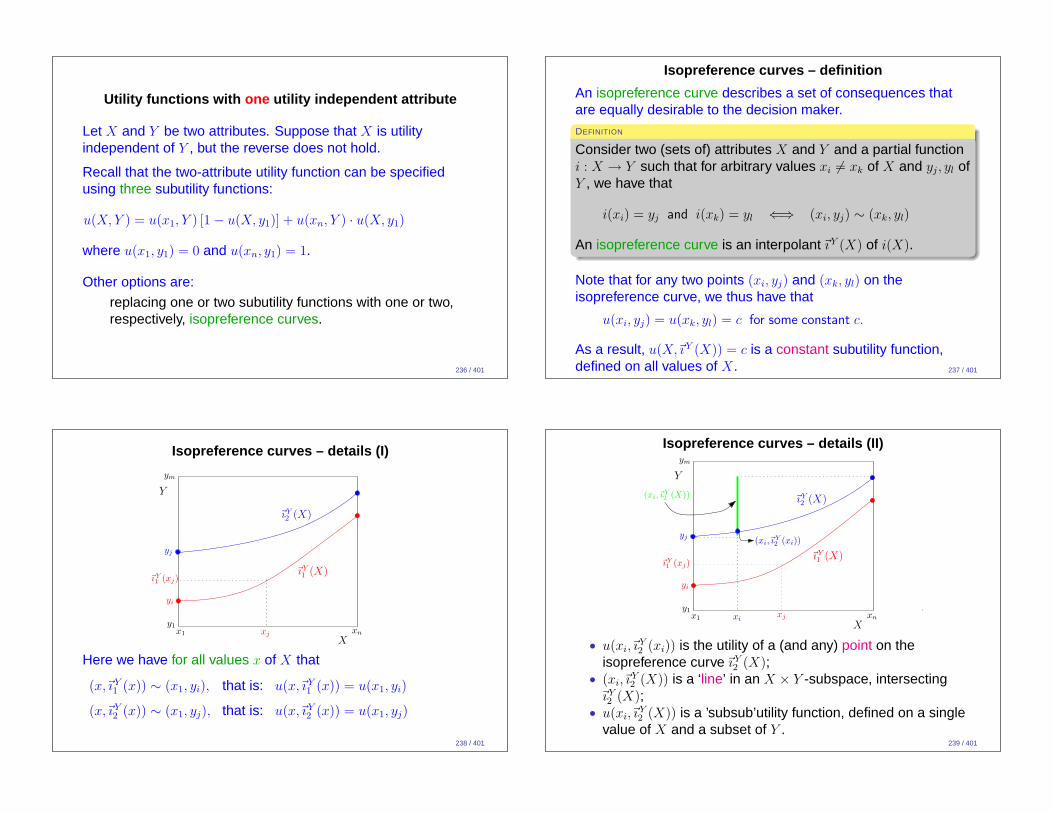
Isopreference curves – details (I)

X

Y

x1 xn

y1

ym

yi

yj

~ıY

2(X)

~ıY

1(X)

xj

~ıY1

(xj)

Here we have for all values x of X that

(x,~ıY1 (x)) ∼ (x1, yi), that is: u(x,~ıY

1 (x)) = u(x1, yi)

(x,~ıY2 (x)) ∼ (x1, yj), that is: u(x,~ıY

2 (x)) = u(x1, yj)

238 / 401

Isopreference curves – details (II)

X

Y

x1 xn

y1

ym

yi

yj

~ıY

2(X)

~ıY

1(X)

xj

~ıY1

(xj)

(xi,~ıY2

(xi))

xi

(xi,~ıY2

(X))

• u(xi,~ıY2 (xi)) is the utility of a (and any) point on the

isopreference curve~ıY2 (X);

• (xi,~ıY2 (X)) is a ‘line’ in an X × Y -subspace, intersecting

~ıY2 (X);

• u(xi,~ıY2 (X)) is a ’subsub’utility function, defined on a single

value of X and a subset of Y .239 / 401

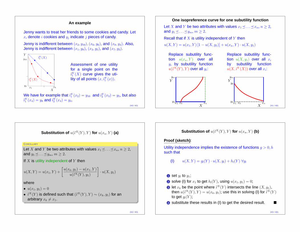
An example

Jenny wants to treat her friends to some cookies and candy. Letxi denote i cookies and yj indicate j pieces of candy.

Jenny is indifferent between (x2, y10), (x6, y6), and (x8, y4). Also,Jenny is indifferent between (x1, y9), (x3, y5), and (x7, y3).

X

Y

x1x8

y2

y10

~ıY

1(X)

~ıY

2(X)

Assessment of one utilityfor a single point on the~ıY1 (X) curve gives the uti-

lity of all points (x,~ıY1 (x)).

We have for example that~ıY1 (x2) = y10 and~ıY

2 (x3) = y5, but also~ıY1 (x4) = y8 and~ıY

2 (x4) = y4.240 / 401

One isopreference curve for one subutility function


Recall that if X is utility independent of Y then


Replace subutility func-tion u(xn, Y ) over allyi by subutility functionu(~ıX(Y ), Y ) over all yi:

X

Y

x1 xny1

ym

xk

Replace subutility func-tion u(X, y1) over all xi

by subutility functionu(X,~ıY (X)) over all xi:

X

Y

x1 xny1

ym

xk

yk

241 / 401

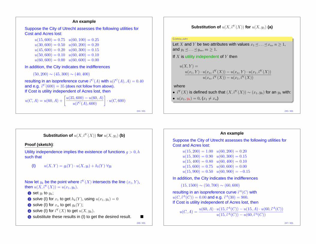
Substitution of u(~ıX(Y ), Y ) for u(xn, Y ) (a)

COROLLARY



u(X,Y ) = u(x1, Y ) +

[

u(xk, y1)− u(x1, Y )

u(~ıX(Y ), y1)

]

· u(X, y1)

where

• u(x1, y1) = 0

• ~ıX(Y ) is defined such that (~ıX(Y ), Y ) ∼ (xk, y1) for anarbitrary xk 6= x1.

242 / 401

Substitution of u(~ıX(Y ), Y ) for u(xn, Y ) (b)

Proof (sketch) :



1 set yl to y1;

2 solve (I) for x1 to get hl(Y ), using u(x1, y1) = 0;

3 let xk be the point where~ıX(Y ) intersects the line (X, y1),then u(~ıX(Y ), Y ) = u(xk, y1); use this in solving (I) for~ıX(Y )to get gl(Y );

4 substitute these results in (I) to get the desired result. �

243 / 401

An example

Suppose the City of Utrecht assesses the following utilities forCost and Acres lost:

u(15, 600) = 0.75 u(60, 100) = 0.25u(30, 600) = 0.50 u(60, 200) = 0.20u(45, 600) = 0.20 u(60, 300) = 0.15u(50, 600) = 0.10 u(60, 400) = 0.10u(60, 600) = 0.00 u(60, 600) = 0.00

In addition, the City indicates the indifferences

(50, 200) ∼ (45, 300) ∼ (40, 400)

resulting in an isopreference curve~ıC(A) with u(~ıC(A), A) = 0.40and e.g. ~ıC(600) = 35 (does not follow from above).If Cost is utility independent of Acres lost, then

u(C,A) = u(60, A) +

[

u(35, 600)− u(60, A)

u(~ıC(A), 600)

]

· u(C, 600)

244 / 401

Substitution of u(X,~ıY (X)) for u(X, y1) (a)

COROLLARY



u(X,Y ) =

u(x1, Y ) · u(xn,~ıY (X))− u(xn, Y ) · u(x1,~ı

Y (X))

u(xn,~ıY (X))− u(x1,~ıY (X))

where

• ~ıY (X) is defined such that (X,~ıY (X)) ∼ (x1, yk) for an yk with:

• u(x1, yk) = 0, (x1 6= xn)

245 / 401

Substitution of u(X,~ıY (X)) for u(X, y1) (b)

Proof (sketch) :



Now let yk be the point where~ıY (X) intersects the line (x1, Y ),then u(X,~ıY (X)) = u(x1, yk).

1 set yl to yk;2 solve (I) for x1 to get hk(Y ), using u(x1, yk) = 0

3 solve (I) for xn to get gk(Y );4 solve (I) for~ıY (X) to get u(X, yk).5 substitute these results in (I) to get the desired result. �

246 / 401

An example


u(15, 200) = 1.00 u(60, 200) = 0.20u(15, 300) = 0.90 u(60, 300) = 0.15u(15, 400) = 0.80 u(60, 400) = 0.10u(15, 600) = 0.75 u(60, 600) = 0.00u(15, 900) = 0.50 u(60, 900) = −0.15


(15, 1500) ∼ (50, 700) ∼ (60, 600)

resulting in an isopreference curve~ıA(C) withu(C,~ıA(C)) = 0.00 and e.g. ~ıA(30) = 900.If Cost is utility independent of Acres lost, then

u(C,A) =u(60, A) · u(15,~ıA(C))− u(15, A) · u(60,~ıA(C))

u(15,~ıA(C))− u(60,~ıA(C))

247 / 401

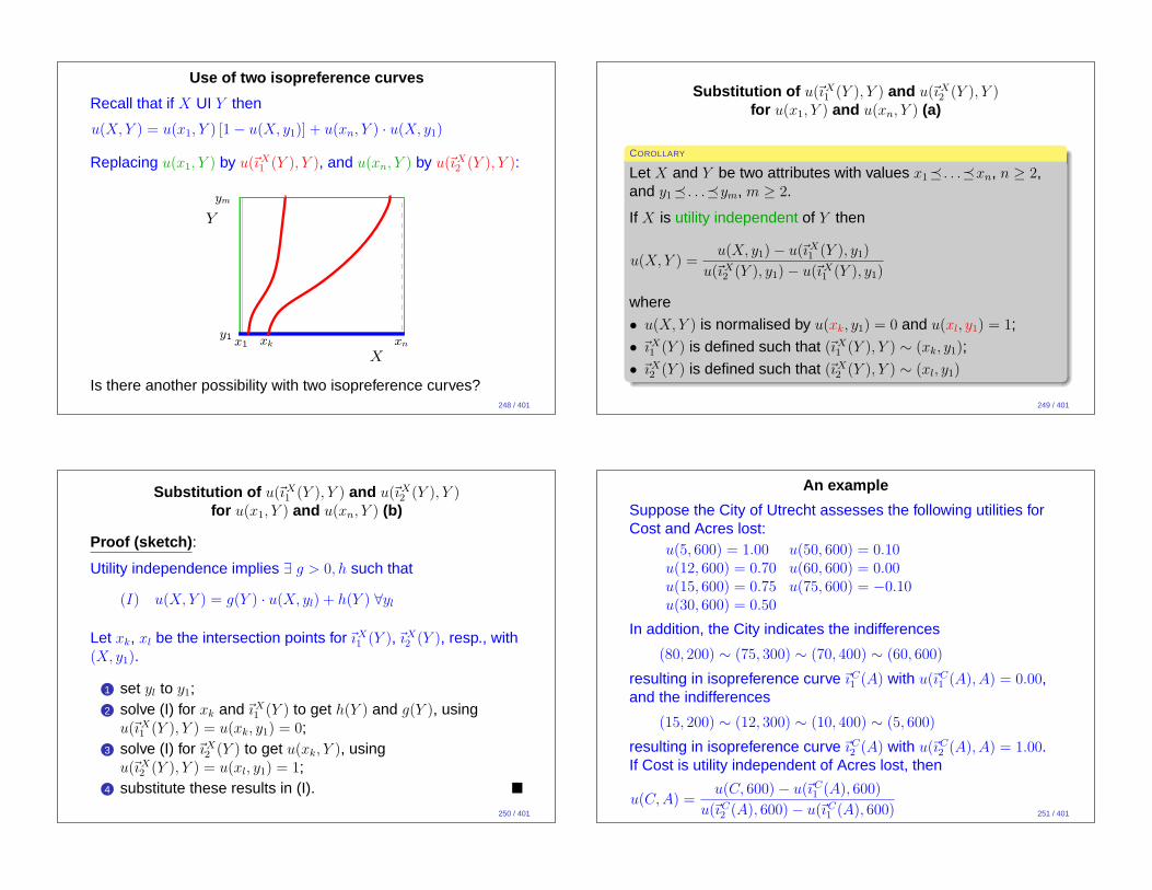
Use of two isopreference curves

Recall that if X UI Y then


Replacing u(x1, Y ) by u(~ıX1 (Y ), Y ), and u(xn, Y ) by u(~ıX

2 (Y ), Y ):

X

Y

x1 xny1

ym

xk

Is there another possibility with two isopreference curves?248 / 401

Substitution of u(~ıX1 (Y ), Y ) and u(~ıX

2 (Y ), Y )for u(x1, Y ) and u(xn, Y ) (a)

COROLLARY



u(X,Y ) =u(X, y1)− u(~ıX

1 (Y ), y1)

u(~ıX2 (Y ), y1)− u(~ıX

1 (Y ), y1)

where

• u(X,Y ) is normalised by u(xk, y1) = 0 and u(xl, y1) = 1;

• ~ıX1 (Y ) is defined such that (~ıX

1 (Y ), Y ) ∼ (xk, y1);

• ~ıX2 (Y ) is defined such that (~ıX

2 (Y ), Y ) ∼ (xl, y1)

249 / 401

Substitution of u(~ıX1 (Y ), Y ) and u(~ıX

2 (Y ), Y )for u(x1, Y ) and u(xn, Y ) (b)

Proof (sketch) :

Utility independence implies ∃ g > 0, h such that

(I) u(X,Y ) = g(Y ) · u(X, yl) + h(Y ) ∀yl

Let xk, xl be the intersection points for~ıX1 (Y ),~ıX

2 (Y ), resp., with(X, y1).

1 set yl to y1;2 solve (I) for xk and~ıX

1 (Y ) to get h(Y ) and g(Y ), usingu(~ıX

1 (Y ), Y ) = u(xk, y1) = 0;3 solve (I) for~ıX

2 (Y ) to get u(xk, Y ), usingu(~ıX

2 (Y ), Y ) = u(xl, y1) = 1;4 substitute these results in (I). �

250 / 401

An example


u(5, 600) = 1.00 u(50, 600) = 0.10u(12, 600) = 0.70 u(60, 600) = 0.00u(15, 600) = 0.75 u(75, 600) = −0.10u(30, 600) = 0.50


(80, 200) ∼ (75, 300) ∼ (70, 400) ∼ (60, 600)

resulting in isopreference curve~ıC1 (A) with u(~ıC

1 (A), A) = 0.00,and the indifferences

(15, 200) ∼ (12, 300) ∼ (10, 400) ∼ (5, 600)

resulting in isopreference curve~ıC2 (A) with u(~ıC

2 (A), A) = 1.00.If Cost is utility independent of Acres lost, then

u(C,A) =u(C, 600)− u(~ıC

1 (A), 600)

u(~ıC2 (A), 600)− u(~ıC

1 (A), 600) 251 / 401

Documents

Multi-attribute utility theory - Utrecht University · Multi-attribute utility theory (very superﬁcial in textbook!) 164 / 401 Multiple objectives – an example Consider the problem