Embed Size (px)
Citation preview
Multi-Armed Bandits, Gittins Index, and Its Calculation
Jhelum Chakravorty and Aditya Mahajan
24
24.1 Introduction
Multi-armed bandit is a colorful term that refers to the di lemma faced by a gambler playing in a casino with multiple slot ma-chines (which were colloquially called one-armed bandits). W h a t strategy should a gambler use to pick the machine to play next? It is the one for which the poste-rior mean of winning is the highest and thereby maximizes current expected re-ward, or the one for which the posterior variance of winning is the highest, and has the potential to maximize the future ex-pected reward. S imi lar exploration vs ex-ploitation trade-offs arise in various appli -cation domains including cl inical tr ials [5], stochastic scheduling [25], sensor manage-ment [33], and economics [4].
C l i n i c a l tr ials fit natural ly into the framework of mult i -armed bandits and have been a motivation for their study since the early work of Thompson [31]. Broadly speaking, there are two ap-proaches to mult i -armed bandits. T h e first, following Bel lman [2], aims to maxi -mize the expected total discounted reward over an infinite horizon. T h e second, fol-
lowing Robbins [27], aims to minimize the rate of regret for the expected total reward over a finite horizon. I n some of the litera-ture, the first setup is called geometric dis-counting while the second is called uniform discounting. For a large time, the mult i -armed bandit problem, in both formula-tions, was considered unsolvable unti l the pioneering work of G i t t ins and Jones [13] for the discounted setup and that of L a i and Robbins [22] for the regret setup char-acterized the nature of the optimal strat-egy.
I n this chapter, we restrict our atten-tion to the discounted setup; we refer the reader to a recent survey by Bubeck and Cesa-Bianchi [9] and references therein for the regret setup and to Kuleshov and Pre-cup [20], who discuss the regret setup in the context of cl inical trials.
24.2 Mathematical Formulation of Multi-Armed Bandits
Mult i -armed bandit ( M A B ) is a sequential decision problem in which, at each time,
416
Methods and Applications of Statistics in Clinical Trials: Planning,Analysis, and Inferential Methods. Edited by N. Balakrishnan.
© 2014 John Wiley & Sons, Inc. Published 2014 by John Wiley & Sons, Inc.
441 Multi-Armed Bandits, Gittins Index, and Its Calculation J^ll
a player must play one among n available bandit process. In the simplest setup, a bandit process is a controlled Markov pro-cess. The player has two controls: ei-ther play the process or not. If the player chooses to play the bandit process 2, i = 1 , . . . , n, the state of the bandit process i evolves in a Markovian manner while the state of all other processes remains frozen (i.e., it does not change). Such a ban-dit process is called a Markovian bandit process. More sophisticated setups assume that when a bandit processes is played, its state evolves according to an arbitrary stochastic process. To focus on the key conceptual ideas, we restrict our attention to Markovian bandit processes. For more general bandit processes, the description of the solution concept and its computation are more involved.
Formally, let { X l } ^ denote the bandit process. The state X\ of the bandit pro-cess i , i = l , . . . , n , takes values in an arbi-trary space X%. For simplicity, we assume in most of the discussion in this chapter that X% is finite or countable.
Let Ut = ( u l , . . . , u t ) denote the deci-sion made by the player at time The component u\ is binary valued and denotes whether the player chooses to play the ban-dit process i (u\ = 1) or not {u\ = 0). Since the player may only choose to play one bandit process at each time, u t must have only one nonzero component, or equiva-lent^
n
= vt. i=1
Let U £ {0, l } n denote all vectors with this property. The collection { K t = { X l , . . . , X t n ) } £ 0 evolves as follows: Vz = 1, ..., n
4 = ( f ( x i w ; ) J if<4 = 1, t + 1 \XL if u\ — 0,
where {W? i = 1 , . . . ,n, are mutually independent i.i.d. processes. Thus, when
u\ = 1, X\ evolves in a Markovian manner; otherwise it remains frozen.
When bandit process i is played, it yields a reward r l ( X l ) and all other pro-cesses yield no reward. The objective of a player is to choose a decision strategy 9 = {9t}%Lo> where gt : [JlLi x i so as
to maximize the expected total discounted reward
oo n
t—0 i=l
where xo = ( x j , . . . , Xq ) is the initial start-ing state of all bandit processes and (3 € (0,1) is the discount factor.
24.2-1 An Example
Consider an adaptive clinical trial with n treatment options. When the tth patient comes for treatment, she may be prescribed any one of the n available options based on the results of the previous trials. The se-quence of success and failure of each treat-ment is an Bernoulli process with an un-known success probability s*, i = 1, ..., n. The objective is to design an adaptive strategy that maximizes the expected total discounted successful treatments.
The above adaptive clinical trial may be viewed as a M A B problem as follows. Suppose the prior distribution of sl has a beta distribution that is independent across treatments. Then the posterior dis-tribution of 5% which is calculated using Bayes' rule, is also a beta distribution, say Beta(pJ,gJ) at time t. Therefore, each treatment may be modeled as a Marko-vian bandit process where the state X\ is (pbQt)i the state update function / cor-responds to Bayes update of the poste-rior distribution, and the reward function rl(X}) = Pt/(Pt + Qt) captures the proba-bility of success.
442 Multi-Armed Bandits, Gittins Index, a n d I t s Calculation J^ll
24.2.2 Solution Concept and lows:
the Gittins Index One possible solution concept for the M A B problem is to set it up as a Markov deci-sion process (MDP) and use Markov de-cision theory [26] to solve it. However, such an approach does not scale well with the number of bandit processes because of the curse of dimensionality. To see this, assume that the state space X1 of each bandit process is a finite set with ra el-ements. Then the state space of the re-sultant MDP, which is the space of real-izations of Xt , has size m n . The solu-tion complexity of solving a M D P is pro-portional to the size of the state space. Hence the complexity of solving M A B us-ing Markov decision theory increases expo-nentially with the number of bandit pro-cesses. A key breakthrough for the M A B problem was provided by Gittins and Jones [13] and Gittins [15], who showed that in-stead of solving the n-dimensional M D P with state-space n l L i > a n optimal solu-tion is obtained by solving n 1-dimensional optimization problems: for each bandit i, i = 1, . . . , n, and for each state xl € X1, compute
E vl(xl) — max -
v ' T> o
£ P r W ) Lt=0 Xio = xi
E t = 0
XK
(!) where r is a {cr(X[,...,X\)}<£Ll measur-able stopping time. The function vl(xl) is called Gittins index of bandit process i at state xl. The optimal r in (1), which is called the optimal stopping time at x\ is given by the hitting time T(S(x1)) of a stopping set S(xl) C X\ t!hat is, the first time the bandit process enters the set S(xl). Algorithms to compute the Gittins index of a bandit process are presented in Section 24.3.
Gittins and Jones [13] and Gittins [15] characterized the optimal strategy as fol-
• At each time, play the arm with the highest Gittins index.
Thus, to implement the optimal strat-egy, compute and store the Gittins index vl(x%) of all states xl € X1 of all bandit processes i, i = 1, ..., n. Off-line algo-rithms that compute the Gittins index of all states of a bandit process are presented in Section 24.3.
An equivalent interpretation of the Git-tins index strategy is the following:
• Pick the arm with the highest Gittins index and play it until its optimal stop-ping time (or equivalently, until it en-ters the corresponding stopping set) and repeat.
Thus, an alternative way to implement the optimal strategy is to compute the Git-tins index vl(x\) and the corresponding stopping time [or equivalently, the corre-sponding stopping set S(x1)] for the cur-rent state x\ of all bandit processes i, i = 1, ..., n. On-line algorithms that compute the Gittins index and the corresponding stopping set for an arbitrary state of a ban-dit process are presented in Section 24.4.
Off-line implementation is simpler and more convenient for bandit processes with finite and moderately sized state space. On-line implementation becomes more convenient for bandit processes with large or infinite state space.
24.2.3 Salient Features of the Model
As explained by Gittins [15], M A B prob-lems admit a simpler solution than gen-eral multistage decision problems because they can be optimally solved with forward induction. In general, forward induction is not optimal and one needs to resort to backward induction to find the optimal strategy. Forward induction is optimal for
443 Multi-Armed Bandits, Gittins Index, and Its Calculation J^ll
M A B setup because it has the following features:
1. The player plays only one bandit pro-cess, and that process evolves in an uncontrolled manner.
2. The processes that are not played are frozen.
3. The current reward depends only on the current state of the process that is played and is not influenced by the state of the remaining processes and the history of previous plays.
Because the above features, decisions made at each stage are not irrevocable and hence forward induction is optimal. On the basis of the above insight, Gittins [15] proved the optimality of the index strat-egy, using an interchange argument. Since then, various other proofs of the Gittins in-dex strategy have been proposed (see [14] for a detailed summary).
Several variations of M A B problems have been considered in the literature. These variations remove some of the above features, and, as such, index strategies are not necessarily optimal for these variations. We refer the reader to the survey by Ma-hajan and Teneketzis [23] and references therein for details on the variations of the M A B problem.
24.3 Off-Line Algorithms for Computing Gittins Index
Since the Gittins index of a bandit process depends just on that process, we drop the label i and denote the bandit process by
o-Off-line algorithms use the following
property of the Gittins index. The Gittins index v : X —» E induces a total order >z on X that is given by
Using this total order, for any state a e X)
the state space X may be split into two sets
C(a) = {b € X : b y a},
5(a) = {b e X : a y b}.
These sets are, respectively, called the con-tinuation set and the stopping set. The rationale behind the terminology is that if we start playing a bandit process in state a, then it is optimal to continue playing the bandit process in all states C(a) because for any b € C(a), u(b) > v(a). Thus, the stopping time that corresponds to starting the bandit process in state a is the hitting time T(5(a)) of set 5(a), that is, the first time the bandit process enters set 5(a). Using this characterization, the expression for Gittins index (1) simplifies to
E
u(a) = max -S(a)CX
r T(S(a))
£ Pr(Xt) t=o
Xq = a
Va, b <E X , ahb v(a) > v(b).
rT(S(a)) E jr P Xo = a
L t—0 (2)
where T(5(a)) = inf{* > 0 : Xt G 5(a)} is the hitting time of set 5(a). The off-line algorithms use this simplified expression to compute the Gittins index.
For ease of exposition, assume that Xt takes values in a finite space X = { 1 , . . . , ra}. Most of the algorithms extend to countable state spaces under appropri-ate conditions. Denote the m x m tran-sition probability matrix corresponding to the Markovian update of the bandit pro-cess by P = [Pa,b] and represent the re-ward function using a ra x 1 vector r, i.e. r a = r (a) . Furthermore, let 1 be the ra x 1 vector of ones, 0 m x i be the ra x 1 vector of zeros, I be the m x m identity matrix, and 0 mxm be the mxm matrix of zeros.
420 Multi-Armed Bandits, Gittins Index, and Its Calculation J^ll
24.3.1 Largest-Remaining-Index Algorithm (Varaiya, Walrand, and Buyukkoc)
Varaiya, Walrand, and Buyukkoc [32] pre-sented an algorithm to compute the Git-tins index, which we refer to as the largest-remaining-index algorithm. The key idea behind this algorithm is to identify the states in X according to the decreasing or-der
where (ai , . . . , a m ) is a permutation of (1, . . . , ra).
The algorithm proceeds as follows:
Ini t ia l izat ion: The first step of the al-gorithm is to identify the state a\ with the highest Gittins index. Since a\ has the highest Gittins index, S(a i ) = X. Sub-stituting this in (2), we get that v(a\) = r(a i ) = r Q l . Then, choose
a\ = arg max ra
where ties are broken arbitrarily. The cor-responding Gittins index is
v{qli) = rai.
Recursion step: After the states ai, . . . , ah-1 have been identified, the next step is to identify the state a k with the kth largest Gittins index. Even though ak is not known, we know that C(ak) = {otu • • •, afe-i} and S(ak) = X \ { a i , . . . , a k - i } . Substituting this in (2), we can compute v(ak) as follows. Define the ra x ra matrix by Va, b G X,
qW = f p a ,6 , if 6 € C(afc), a'6 [0, otherwise;
and define the ra x 1 vectors:
d(*> = [I —
(3)
(4)
Then, choose
a k = arg max
where ties are broken arbitrarily. The cor-responding Gittins index is
d(*) b w
Computational complexity: The per-formance bottleneck of this algorithm is the two systems of the linear equations (4) that need to be solved at each step. At step fc, each system effectively has k variables, so solving each requires (2/3)fc3 + 0(k2) arithmetic operations. Thus, overall this algorithm requires
m 2j2[lk3 + 0(k2)] ^ i r a 4 + 0 ( m 3 )
k=l
arithmetic operations. This algorithm has the worst computational complexity of all the algorithms presented.
E x a m p l e 24 .3 .1 Consider a bandit pro-cess with state space X = {1 ,2,3,4}, re-ward vector r = [16 19 30 4]T, and probability transition matrix
0.1 0 0 .8 0.1 0.5 0 0 .1 0.4 0.2 0.6 0 0.2 0 0.8 0 0.2
Let the discount factor be f3 = 0.75. Using the largest-remaining-index algo-
rithm, the Gittins index for this bandit process is calculated as follows:
Init ia l izat ion: Start by identifying the state with the highest Gittins index:
ai = arg max ra = 3; adzX
v{ol\) = r3 = 30.
445 Multi-Armed Bandits, Gittins Index, and Its Calculation J^ll
R e c u r s i o n s t e p :
1. S t e p k = 2: Although ct2 is not known, we know that C(a2) = {3} and S(a2) = { 1 ,2 ,4} . Using (3) and (4) we get
o(2) 0 0 0 . 8 0 0 0 0.10 00 0 0 00 0 0
"34 " •1.6 _
21.25 30 4
, b<2> = 1.075 1 1
Hence,
3.
d ( 2 ) a 2 = arg max = 1;
v(ol2) = d ( 2 )
"a2 : 21.25.
2. S t e p k = 3: Although <23 is not known, we know that C(a3) = { 1 , 3 } and S ( a 3 ) = {2,4}. Using (3) and (4) we get
o ( 3 ) -0 . 1 0 0 . 8 0 1 0.5 0 0.10 0.20 0 0 0 0 0 0
d<3> =
Hence,
"40.719" "1.916" 36.977 , b<3> = 1.815 36.108 , b<3> = 1.288 4 1
is(a3) =
d(a3) arg max - j r r
a€{2,4} b ( 3 )
i(3) d«3_ kp)
20.372.
S t e p fc = 4: As before, although c*4 is not known, we know that C(a4) = { 1 , 2 , 3 } and S(a4) = {4}. As in the previous steps, using (3) and (4) we get
o(4) 0.1 0 0.80 0.5 0 0.10 0.2 0.6 0 0 0 0.8 0 0
Since S(a4) = ment, we have
"54.929" " 2.613" 43.95 , b<4> = 2.157 58.017 , b<4> = 2.363
.30.371. 2.295
{4} has only one ele-
04 = 4, and v(a±) d ( 4 )
Hi) Wa4 13.236.
Thus, the vector of the Gittins index of this bandit process is
v = 21.25 20.372 30 13.236
24.3.2 State-Elimination Algorithm (Sonin)
Sonin [30] presented an algorithm to com-pute the Gittins index, which we refer to as the state-elimination algorithm. As with the largest-remaining-index algorithm, the main idea behind the state-elimination al-gorithm is to iteratively solve (2) in the decreasing order of K The computations are based on a relation of (2) with optimal stopping problems [29].
A simplified version of the state-elimina-tion algorithm is presented below. See [30] for a more efficient version that also works when the discount factor (3 depends on the state.
Ini t ia l izat ion: The initialization step is identical to that of the largest-remaining-index algorithm: Identify the state a i with highest Gittins index, which is given by
Oil arg m a x r a
where ties are broken arbitrarily. The cor-responding Gittins index is
V(ol{) L c*l • Step k of the recursion uses a mxm
matrix and rax 1 vectors a w and b (*> , where ra = |5(a /e)| = ra-fc-f 1 . These are initialized as Q^1) = P , d^1) = r, and b(!) = ( 1 - / 3 ) 1 .
446 Multi-Armed Bandits, Gittins Index, and Its Calculation J^ll
Recursion step: After the states ai, . . . , a/e-i have been identified, the next step is to identify the state a k with the kth largest Gittins index. Even though ak is not known, we know that C(ak) = { a i , . . . , ajb-i} and S{ak) = X \ { a i , . . . , a k - i } . Let the model in the step k- 1 be Q ^ " 1 ) , d ^ " 1 ) and b ^ " 1 ) . Define
A/c-i = 0 1 _ tfQ^-1) ajb-i
Let fa = |5(afe)|- Define rax fa matrix by Va,b£S(ak):
o(fc ) - Q i V ^ - i Q ^ Q (fe-i) atk-i,b'
(5) and define rax 1 vectors by Va E S(ak)
(6 )
Note that the entries of Q<-kK d<fc> and are labeled according to the set S(ak). For example, if X — {1 ,2,3}, a i = 2 then S ( a i ) = {1 ,3} and
d ( 2 )
Q<2> =
r a < 2 > !
a2>
0 ( 2 > q ( 2 ) 1 Wi 3 Qft Q&
and b<2> bS2)
2 arithmetic operations [since we can pre-COmpute Xk-lQaHakhi f° r a € S(otk) before updating Q(&)]. Thus, overall this algorithm requires
m ] T [2(ra-fc-f l)2 -f O(fc)] = | m 3 + 0 ( m 2 ) k=l
arithmetic operations. Our calculations differ from the ra3 -f 0(ra2) calculations reported in [24] because [24] assumes that the update of each element of Q ^ takes 3 arithmetic operations, but, as we argued above, this update can be done in 2 op-erations if we pre-multiply row a k - i of
with Afc-i. Furthermore, in the implementation presented in [24], b^) is computed from requiring additional 0(ra2) arithmetic operations. The above implementation avoids those by keeping track of b^k\
Example 24.3.2 Reconsider the bandit process of Example 24.3.1. Using the state-elimination algorithm, the Gittins index for this bandit process is calculated as fol-lows.
Ini t ia l izat ion: Start by identifying the state with the highest Gittins index:
After calculating and choose
d{ak)
a k = arg max - ^ r
where ties are broken arbitrarily. The cor-responding Gittins index is
u ( a k ) = ( ! - / ? )
d(k) qafc b w
a\ — arg max r a
u{a i) = r 3 = 30.
Initialize:
Q(«
d ( i )
3;
0.1 0 0 . 8 0 . 1 0.5 0 0.1 0.4 0 .2 0.6 0 0 .2 0 0.8 0 0.2
-16" "0.25" 19 30 , = 0.25
0.25 4 0.25
Computational complexity: The per-formance bottleneck of this algorithm is the update of matrix Q ^ at each step. In step fc, the matrix Q W has (ra—fc+1)2 ele-ments and update of each element requires
Recursion step:
1. Step k = 2: Although a 2 is not known, we know that C(a2) is {3}, S(a2) = {1,2,4}, and Ax - 0/(1 -
447 Multi-Armed Bandits, Gittins Index, and Its Calculation J^ll
(3qW ) = 0.75. Using (5) and (6) we get
Q®
1 2 4 0.22 0.36 0.22 0.515 0.045 0.415
0 0.8 0.2 .
Since 5(04) = {4} has only one ele-ment, we have
Q4 = 4, and
d(4) i/(a4) = ( l - 0 ) ^ = 13.236.
34 , v 1 " 0.4 " 21.25 , b<2> = 2 0.269 24.3.3
4 4 . 0.25 .
Hence,
di2) a 2 = arg max - ^ r = 1;
j V(Q2) = ( 1 - / 3 ) 5 ^
(2) o bl2
21.25.
2. Step ft = 3: Although 0:3 is not known, we know that C(a3) = {1 ,3} , 5 ( o 3 ) = {2,4}, and A2 = 0/(1 -0 Q $ ) = 0.898. Using (5) and (6) we get
q ( 3 ) = 2
4
2 4 0.21 0.52 0.8 0.2
d<3> = 2 36.98 , b<3> = 2 0.45 4 4 ' 4 0.25_
Hence,
d(3) O-a a 3 = arg max = 2;
d(3) i/(a3) = = 20.372.
ba3
3. Step k = 4: Although 04 is not known, we know that C(a4) = {1,2,3}, 5(0:4) = {4}, and A3 = (3/(1 - 0 Q ^ ) = 0.882. As in the pre-vious steps, using (5) and (6) we get
4 4 [ 0.5691
d ^ = 4 [30.37], b<4>= 4 [0.574].
Triangularization Algo-rithm (Denardo, Park, and Rothblum)
Denardo, Park, and Rothblum [12], inde-pendently of Sonin, presented an algorithm that is similar to the state-elimination al-gorithm. We refer to this algorithm as the triangularization algorithm. Although the main motivation for this algorithm was to compute the performance of any index strategy, it can be used to compute the Git-tins index as well.
A slightly modified version of the trian-gularization algorithm is presented below. See [12] for the original version.
In i t i a l i za t ion : The initialization step is identical to the previous two algorithms: Identify the state a\ with the highest Git-tins index, which is given by
a\ = arg max r a a£X
where ties are broken arbitrarily. The cor-responding Gittins index is
V(oli) =rftl.
The recursion step uses a ra x (ra 4- 2) tableau
= [Q<fc>|d<fe>|b<fe>]
where Q ^ is a ra x ra square matrix and d W and b ^ are ra x 1 vectors. Initialize these as Q W = I - 0 P , d ^ = r, and b W = ( 1 - / 3 ) 1 .
448 Multi-Armed Bandits, Gittins Index, and Its Calculation J^ll
Recursion step: After the states . . . , a k - i have been identified, the next step is to identify the state a k with the fcth largest Gittins index. As before, even though a k is not known, we know that C(otk) = { a i , . . . , a/c-i} and S(ak) = X \ { a i , . . . , a k ~ 1}. Suppose the tableau in step A; — 1 is
M ( / c - 1 ) - [ q C * - 1 * I d ^ - 1 ) I b ^ - 1 ) ] .
Update this tableau using the following el-ementary row operations
1. Let A/c-i = 1 /QofcZi^afc-i• Scale row a k ~ i of tableau M ^ - 1 ) by A^-i [i.e., rescale row a k - i such that the (ak-i,ak-i) entry of M ^ " 1 ) is 1].
2. For each state a G S(ak), subtract row ak-i times the constant Q^afe_i from row a [these operations set Q ^ to 0 for b G C(ak)]. The updated tableau is M<*).
After updating the tableau, choose
d(ak)
a k = arg max - j r r
where ties are broken arbitrarily. The cor-responding Gittins index is
Ak)
Computational complexity: The per-formance bottleneck of this algorithm is the elementary row operations performed at each step to update the tableau. In step fc, this algorithm performs (ra — fc + 2) row operations and each row operation requires 2(ra — fc -f- 1) arithmetic opera-tions [This is because columns correspond-ing to C(ak-1) need not be updated be-cause Q^afe-i is 0]. Thus, overall the algo-rithm requires
m ] T [2(ra - fc -f l)(ra - fc + 2) + 0(fc2)] k—1
= |ra3 + 0(ra2)
arithmetic operations.
Example 24.3.3 Reconsider the bandit process of Example 24.3.1. Using the tri-angularization algorithm, the Gittins index for this bandit process is calculated as fol-lows:
Init ia l izat ion: As in the other two algo-rithms, the state with the highest Gittins index is
a i — arg max ra = 3; a€X
v(ai) = 30.
Initialize the tableau M ^ as • 0.925 0 - 0 . 6 - 0 . 0 7 5 16 0.25"
- 0 . 3 7 5 1 - 0 . 0 7 5 - 0 . 3 19 0.25 - 0 . 1 5 - 0 . 4 5 1 - 0 . 1 5 30 0.25
0 - 0 . 6 0 0.85 4 0.25
Recursion step: 1. Step k = 2: Since a\ = 3, set
Ai = I/Q33 = 1. Using the elemen-tary row operations, the tableau M^2) is updated to
" 0.835 - 0 . 2 7 0 - 0 . 1 6 5 34 0.4 " - 0 . 3 8 6 0.966 0 - 0 . 3 1 1 21.25 0.269 - 0 . 1 5 - 0 . 4 5 1 - 0 . 1 5 30 0.25
0 - 0 . 6 0 0.85 4 0.25
Hence,
di2)
a 2 = arg max = 1; a€{l,2,4} bi2)
d ( 2 )
i/(a2) = ( l - / ? ) - ^ = 21.25.
2. Step k = 3: Since a2 = 1, set A2 = 1/Qi^i = 1.198. Using the el-ementary row operations, the tableau M^3) is updated to
• 1 - 0 . 3 2 3 0 - 0 . 1 9 8 40.719 0.479" 0 0.841 0 - 0 . 3 8 8 36.978 0.454
- 0 . 1 5 - 0 . 4 5 1 - 0 . 1 5 30 0.25 0 - 0 . 6 0 0.85 4 0.25
449 Multi-Armed Bandits, Gittins Index, and Its Calculation J^ll
Hence,
d ( 2 ) a 2 = arg max -£rr = 2;
«e{2.4} bi2)
v(a3) = (1 - 0) d(3)
k ( . 3 ) 20.362.
3. Step ft = 4: Since as = 2, set A3 = 1 / Q ^ = 1.189. Using the el-ementary row operations, the tableau M ( 4 ) is updated to
• 1 -0 .323 0 -0 .198 40.72 0.479" 0 1 0 -0 .461 43.95 0.539
-0 .15 -0 .45 1 - 0 . 1 5 30 0.25 0 0 0 0.574 30.37 0.574
Since S(a4) = {4} has only one ele-ment, we have
c*4 = 4 and
d(4) i/(a4) = ( 1 - / ? ) - ^ - 13.236.
24.3.4 Fast-Pivoting Algorithm (Nino-Mora)
Nino-Mora [24] presented an algorithm to compute the Gittins index that refines a previous algorithm proposed by Kallen-berg [16]. We refer to this algorithm as the fast-pivoting algorithm. As with the other algorithms, the main idea behind the fast-pivoting algorithm is to iteratively solve (2) in the decreasing order of K The compu-tations are based on a relation of (3) with marginal productivity rate [24].
A modified version of the algorithm is presented below. See [24] for the original version.
In i t i a l i za t ion : The initialization step is identical to the previous three algorithms: identify the state ot\ with the highest Git-tins index, which is given by
a\ = arg m a x r 0
where ties are broken arbitrarily. The cor-responding Gittins index is
i/(a 1) L ai •
The recursion step uses a m x m matrix and rax 1 vectors b ^ and S k \ where
ra == |£(a/c)| = m — k -f 1. Initialize these as Q « = 0 m x m , b*1) = 1, dW = r.
Recursion step: After the states have been identified, the
next step is to identify the state ak with the fcth largest Gittins index. Even though ak is not known, we know that C(ak) = { a i , . . and S(ak) = X \ { a i , . . . , a f c - i } . Let the model in the step k — 1 be Q ^ - 1 ) , b ^ " 1 ) and d ^ " 1 ) and let ra = \S(ak)\.
Define the (ra 4- 1) x 1 vector by Va e S(ak-1),
Let
a,ak-1
A k-
- £
b€C(ak)
P
l - M t ^ '
(*"l)Pl
(7)
Define the m x m matrix by Va G S(ak) tmdb e X\{ak-i},
= -Afe-ihi*-1). (8)
and the ra x 1 vectors by Va € S(ak)
b W ^ b ^ + A f c - x h i ^ b ^ . ' 0 )
d(fe) _ d ( f e - i ) _ u a uafc_ 1 u(fc-1)
"a uc*fc_i ^a
(10)
After the model has been updated, choose
OLk arg max d ^ a€S(afc) a
and the corresponding Gittins index is given by
«/(«*) = d&>.
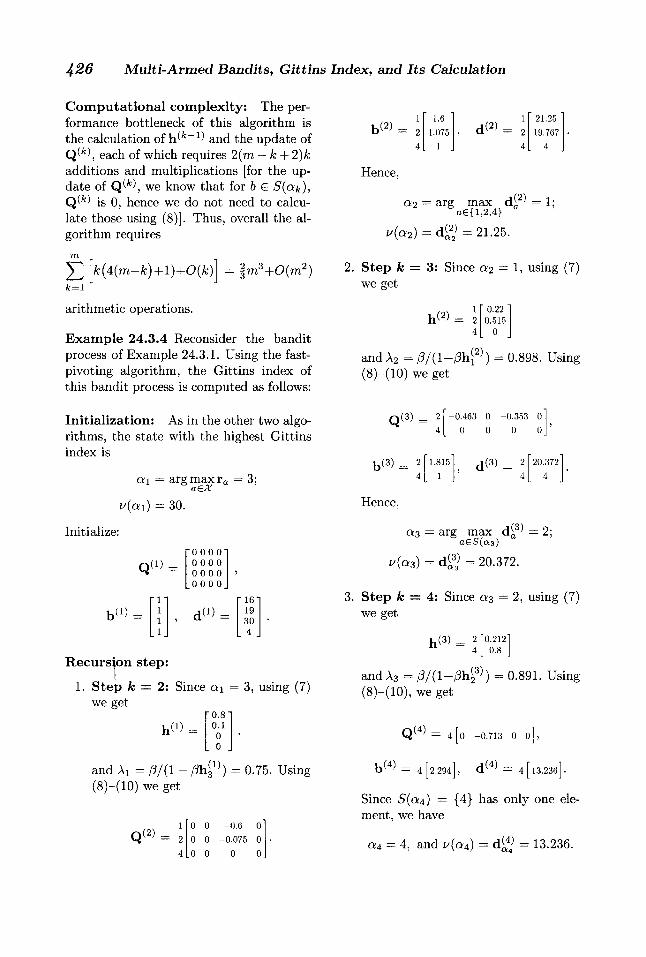
426 Multi-Armed Bandits, Gittins Index , and Its Calculation J^ll
Computational complexity: The per-formance bottleneck of this algorithm is the calculation of h ^ " 1 ) and the update of Q(k\ each of which requires 2(m — k + 2)k additions and multiplications [for the up-date of Q ^ , we know that for b € S(otk), Q i s 0, hence we do not need to calcu-late those using (8)]. Thus, overall the al-gorithm requires
Hence,
1 = 2
1.6 1.075 , d<2>
1 = 2
* 21.25 " 19.767
4 1 4 4
a2 : = arg ; max
o€{ l ,2 ,4} d(2) = i;
/(a2) = = 21.25.
[fe(4(m-ife)+l)+0(Jfe)] = |m 3 +0(m 2 ) l
arithmetic operations.
E x a m p l e 24.3 .4 Reconsider the bandit process of Example 24.3.1. Using the fast-pivoting algorithm, the Gittins index of this bandit process is computed as follows:
Init ial ization: As in the other two algo-rithms, the state with the highest Gittins index is
a \ — arg max ra = 3;
u(a i) = 30.
Initialize:
Q ( i )
0 000 0000 0000 0000
- 1 - " 16" 1 1 , d « = 19
30 . 1 . 4
b<l)
Recursion step:
1. S t e p k = 2: Since a\ = 3, using (7) we get
h(D ro.s
0 .1 0 0
and Ai =/?/(l (8)-(10) we get
0.75. Using
Q (2) 0 0 -0 .6 0
0 0 -0.075 0 0 0 0 0
2. S t e p k = 3: Since a 2 = using (7) we get
h < 2 > = 2 4
0.22 0.515
0
and A2 = /?/(l—/?h^2)) = 0.898. Using (8)—(10) we get
Q (3) -0.463 0 -0.353 0 0 0 0 0
b ( 3 ) = 2 1.815
CM II
co TJ 20.372 4 1 4 4
Hence,
as = arg max d̂ 3̂ = 2; a£S(a 3)
u(as) = di3) = 20.372.
3. S t e p k == 4: Since as = 2, using (7) we get
v,(3) _ 2 [0.212 1 1 4 0.8
and A3 = /?/(l-/?h£3)) = 0.891. Using (8)-(10), we get
Q ( 4 ) = 4 [0 -0.713 0 0],
t / 4 ) = 4 [2.294], d ^ = 4 [ 13.236]-
Since 5(0:4) = {4} has only one ele-ment, we have
a4 = 4, and i/(a4) = = 13.236.
451 Multi-Armed Bandits, Gittins Index, and Its Calculation J^ll
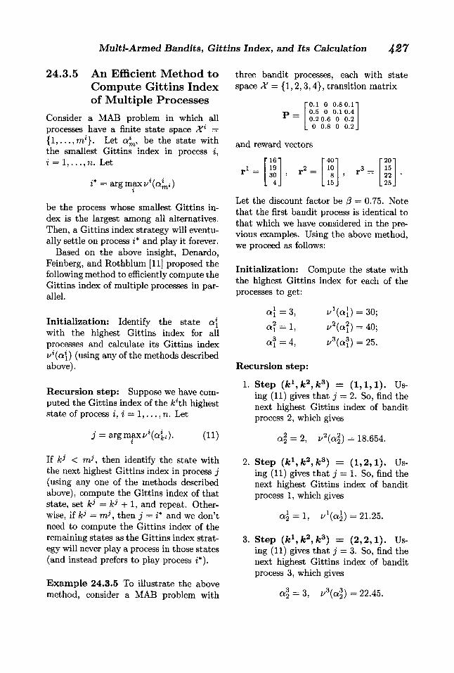
24.3.5 An Efficient Method to Compute Gittins Index of Multiple Processes
Consider a MAB problem in which all processes have a finite state space X1 — { l , . . . , ra*} . Let almi be the state with the smallest Gittins index in process i, i = 1 , . . . ,n. Let
i* = argmaxz/^^i) i
be the process whose smallest Gittins in-dex is the largest among all alternatives. Then, a Gittins index strategy will eventu-ally settle on process i* and play it forever.
Based on the above insight, Denardo, Feinberg, and Rothblum [11] proposed the following method to efficiently compute the Gittins index of multiple processes in par-allel.
Init ial ization: Identify the state a\ with the highest Gittins index for all processes and calculate its Gittins index v%{ol\) (using any of the methods described above).
Recursion step: Suppose we have com-puted the Gittins index of the k%th highest state of process i, i — 1 , . . . , n. Let
three bandit processes, each with state space X — {1,2,3,4}, transition matrix
0.1 0 0 .80 .1 0.5 0 0.10.4 0.2 0.6 0 0.2 0 0.8 0 0.2
and reward vectors _16" -40- "20"
19 r 2 - 10 r 3 _ 15 30 8 5 1 — 22
4 15 25
Let the discount factor be /? = 0.75. Note that the first bandit process is identical to that which we have considered in the pre-vious examples. Using the above method, we proceed as follows:
Init ial ization: Compute the state with the highest Gittins index for each of the processes to get:
= 3 ,
4,
v \ a \ ) = 30;
u \ a l ) = 40;
a? u6{a\) = 25.
Recursion step:
j = a x g m a x i / ' ( < 4 « ) - (11)
1. Step (fc\fc2,ft3) = (1 ,1 ,1) . Us-ing (11) gives that j = 2. So, find the next highest Gittins index of bandit process 2, which gives
a\ = 2, v2[a\) = 18.654.
If y < raJ , then identify the state with the next highest Gittins index in process j (using any one of the methods described above), compute the Gittins index of that state, set fcJ = + 1, and repeat. Other-wise, if fcJ = mJ, then j = i* and we don't need to compute the Gittins index of the remaining states as the Gittins index strat-egy will never play a process in those states (and instead prefers to play process i*).
E x a m p l e 24.3 .5 To illustrate the above method, consider a MAB problem with
2. Step ( fc 1 ,* 2 ,* 8 ) = (1 ,2 , 1) . Us-ing (11) gives that j = 1. So, find the next highest Gittins index of bandit process 1, which gives
a\ 1, vl(a\) — 21.25.
3. Step (fc^fe2,*8) = (2 ,2 , 1) . Us-ing (11) gives that j = 3. So, find the next highest Gittins index of bandit process 3, which gives
a) = 3, v3(al) = 22.45.
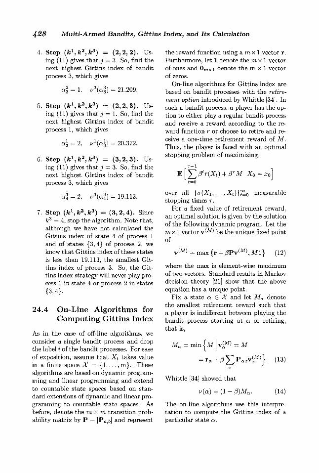
428 Multi-Armed Bandits, Gittins Index, and Its Calculation J^ll
4. Step (fc\fc2,fc8) = (2,2 ,2). Us-ing (11) gives that j = 3. So, find the next highest Gittins index of bandit process 3, which gives
<4 1, i/3(al) = 21.209.
5. Step (fc1, fc2, A;3) = (2 ,2 ,3) . Us-ing (11) gives that j = 1. So, find the next highest Gittins index of bandit process 1, which gives
2, vl(a\) = 20.372.
6. Step (fc\fc2,fc3) = (3 ,2 ,3) . Us-ing (11) gives that j = 3. So, find the next highest Gittins index of bandit process 3, which gives
al = 2, v3(a34) = 19.113.
7. Step (fc1, fc2, fc3) == (3 ,2 ,4) . Since ks = 4, stop the algorithm. Note that, although we have not calculated the Gittins index of state 4 of process 1 and of states {3,4} of process 2, we know that Gittins index of these states is less than 19.113, the smallest Git-tins index of process 3. So, the Git-tins index strategy will never play pro-cess 1 in state 4 or process 2 in states {3,4}.
24.4 On-Line Algorithms for Computing Gittins Index
As in the case of off-line algorithms, we consider a single bandit process and drop the label i of the bandit processes. For ease of exposition, assume that Xt takes value in a finite space X — { 1 , . . . , m). These algorithms are based on dynamic program-ming and linear programming and extend to countable state spaces based on stan-dard extensions of dynamic and linear pro-gramming to countable state spaces. As before, denote the ra x ra transition prob-ability matrix by P = [Pa,b] and represent
the reward function using a ra x 1 vector r. Furthermore, let 1 denote the ra x 1 vector of ones and 0 m x i denote the rax 1 vector of zeros.
On-line algorithms for Gittins index are based on bandit processes with the retire-ment option introduced by Whittle [34]. In such a bandit process, a player has the op-tion to either play a regular bandit process and receive a reward according to the re-ward function r or choose to retire and re-ceive a one-time retirement reward of M . Thus, the player is faced with an optimal stopping problem of maximizing
r - l
t—0 X0 = xq
over all { c r ( X i , . . . , Xt)}^L0 measurable stopping times r .
For a fixed value of retirement reward, an optimal solution is given by the solution of the following dynamic program. Let the ra x 1 vector be the unique fixed point of
r(M) max{r- f /?Pv ( M ) ,Ml} (12)
where the max is element-wise maximum of two vectors. Standard results in Markov decision theory [26] show that the above equation has a unique point.
Fix a state a € X and let Ma denote the smallest retirement reward such that a player is indifferent between playing the bandit process starting at a or retiring, that is,
Mr Q. = min | M W = M
r a + p J 2 v « A M ) } . (13) X
Whittle [34] showed that
i/(a) = (1 -p)Ma. (14)
The on-line algorithms use this interpre-tation to compute the Gittins index of a particular state a.
453 Multi-Armed Bandits, Gittins Index, and Its Calculation J^ll
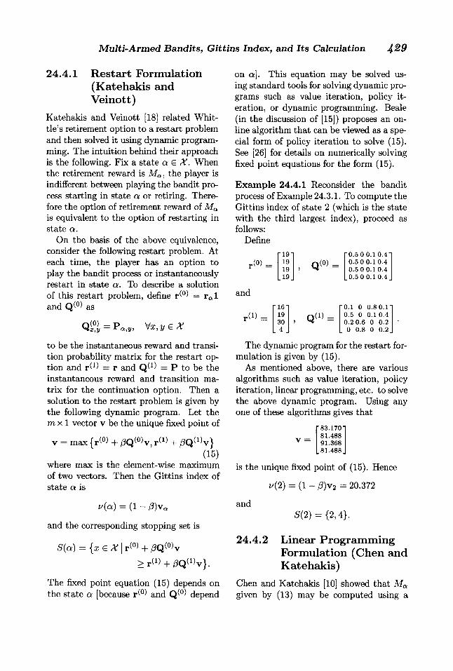
24.4.1 Restart Formulation (Katehakis and Veinott)
Katehakis and Veinott [18] related Whit-tle's retirement option to a restart problem and then solved it using dynamic program-ming. The intuition behind their approach is the following. Fix a state a € X. When the retirement reward is Ma, the player is indifferent between playing the bandit pro-cess starting in state a or retiring. There-fore the option of retirement reward of Ma
is equivalent to the option of restarting in state a .
On the basis of the above equivalence, consider the following restart problem. At each time, the player has an option to play the bandit process or instantaneously restart in state a . To describe a solution of this restart problem, define = r a l and Q(°) as
QS!l = Pa,v, V x , P 6 X
to be the instantaneous reward and transi-tion probability matrix for the restart op-tion and r^1) = r and Q ^ = P to be the instantaneous reward and transition ma-trix for the continuation option. Then a solution to the restart problem is given by the following dynamic program. Let the rax 1 vector v be the unique fixed point of
v = max {r<°> + /?Q(0)v, r ^ + /3Q<1>v} (15)
where max is the element-wise maximum of two vectors. Then the Gittins index of state a is
v{a) = (1 - /?)vtt
and the corresponding stopping set is
S(a) = {xeX\ r<°> + /?Q(0)v >rW + /3Q(1)v}.
The fixed point equation (15) depends on the state a [because r̂ 0̂ and Q(°) depend
on a]. This equation may be solved us-ing standard tools for solving dynamic pro-grams such as value iteration, policy it-eration, or dynamic programming. Beale (in the discussion of [15]) proposes an on-line algorithm that can be viewed as a spe-cial form of policy iteration to solve (15). See [26] for details on numerically solving fixed point equations for the form (15).
Example 24.4.1 Reconsider the bandit process of Example 24.3.1. To compute the Gittins index of state 2 (which is the state with the third largest index), proceed as follows:
Define
and
"19" "0.500.1 0.4" p(°) = 19
19 19
, Q ( 0 ) = 0.5 0 0.1 0.4 0.5 0 0.10.4 0.5 0 0.10.4
"16" "0.1 0 0.80.1" 19
, Q ( 1 ) = 0.5 0 0.1 0.4
30 , Q ( 1 ) = 0.2 0.6 0 0.2 4 0 0.8 0 0.2
r ( i ) =
The dynamic program for the restart for-mulation is given by (15).
As mentioned above, there are various algorithms such as value iteration, policy iteration, linear programming, etc. to solve the above dynamic program. Using any one of these algorithms gives that
83.170 81.488 91.368 81.488
is the unique fixed point of (15). Hence
i/(2) = (1 - P)v2 = 20.372
and 5(2) = {2,4}.
24.4.2 Linear Programming Formulation (Chen and Katehakis)
Chen and Katehakis [10] showed that Ma
given by (13) may be computed using a
430 Multi-Armed Bandits, Gittins I n d e x , and Its Calculation J^ll
linear program. A modified version of this linear program is presented below.
Define h = 1 — e a , where e a is the ra x 1 unit vector with 1 at the ath position. Let diag(h) denote the ra x ra diagonal matrix with h as its diagonal. Let the (m + 1) x 1 vector z = [ y T | z]T, where y is a ra x 1 vector and z is a scalar, be the solutions of the following linear program.
minimize [ ( 1 - / ? ) ( 1 ) t | m]
(16)
subject to
[diag(h) — /3P | l ] z > r,
y > o m x X ,
z unrestricted.
Then the Gittins index of state a is
u(a) = z
and the corresponding stopping set is
S{a) = {xeX |y* = 0}. The linear program (16) depends on the state a (because h depends on a). This linear program may be solved using stan-dard tools. See [6] for details.
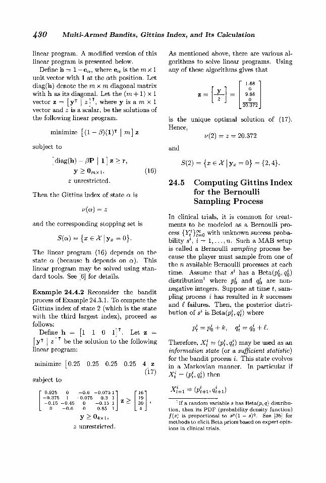
E x a m p l e 2 4 . 4 . 2 Reconsider the bandit process of Example 24.3.1. To compute the Gittins index of state 2 (which is the state with the third largest index), proceed as follows:
Define h - [l 1 0 l ] T . Let z = [ y T | zJ T be the solution to the following linear program:
minimize [0.25 0.25 0.25 0.25 4] z (17)
subject to
0.925 0 - 0 . 6 - 0 . 0 7 5 1" " 16' - 0 . 3 7 5 1 - 0 . 0 7 5 - 0 . 3 1
z > 19
- 0 . 1 5 - 0 . 4 5 0 - 0 . 1 5 1 z > 30 0 - 0 . 6 0 0.85 1 . 4
As mentioned above, there are various al-gorithms to solve linear programs. Using any of these algorithms gives that
1.68 0
9.88 0
20.372
y > o 4 x i , z unrestricted.
is the unique optimal solution of (17). Hence,
i/(2) = z = 20.372
and
S( 2) = { x e X \ y x = 0}={2A}-
24.5 Computing Gittins Index for the Bernoulli Sampling Process
In clinical trials, it is common for treat-ments to be modeled as a Bernoulli pro-cess o with unknown success proba-bility sl, i = 1 , . . . , n. Such a M A B setup is called a Bernoulli sampling process be-cause the player must sample from one of the n available Bernoulli processes at each time. Assume that sl has a Beta(po? <7o) distribution1 where pl
0 and qfa are non-negative integers. Suppose at time t, sam-pling process i has resulted in k successes and I failures. Then, the posterior distri-bution of sl is Beta(pJ, q\) where
Pt=Po + k> Qt =Qo+Z-
Therefore, X\ = (pliQt) may used as an
information state (or a sufficient statistic) for the bandit process i. This state evolves in a Markovian manner. In particular if X} = (p lq i ) then
xIf a random variable s has Beta(pyq) distribu-tion, then its PDF (probability density function) f(s) is proportional to s p ( l — s)q. See [36] for methods to elicit Beta priors based on expert opin-ions in clinical trials.
455 Multi-Armed Bandits, Gittins Index, and Its Calculation J^ll
= J(Pt + i><??), w.p. pj/(pj + ®J); + w.p.
where w.p. is an abbreviation for "with probability." The average reward on playing process i is the mean value of B e t a ( p \ , q \ ) , that is,
Pt Pt + Qt
In this section, we describe the various al-gorithms to compute the Gittins index of such a Bernoulli sampling process. As be-fore, since the computation of the index depends only on that process, we drop the label i and denote the sampling process by {(Pt,Qt)}frLo a n ( l *ts Gittins index by u(p, q).
The main difficulty in computing the Gittins index i/(p, q) is that the state space X = is countably infinite. Hence, an exact computation of the index is not pos-sible. In this section we present algorithms that compute the Gittins index with arbi-trary precision by restricting to a truncated state space Xl = {(p, q) \ p + q < L} for sufficiently large value of L. The results based on these calculations are tabulated in [14]. Different approximations to z/(p, q) have also been proposed in the literature, and we describe a few of these in this sec-tion as well.
24.5.1 Dynamic Programming Formulation (Gittins)
Gittins [14] used the dynamic program-ming formulation of Whittle's retirement option [34], which was presented in Sec-tion 24.4, to compute the Gittins index z/(p, q). In the case of a Bernoulli sampling process, the dynamic program (12) simpli-fies to
+ + 1).
Let Mp q̂ be defined as in (13). Then, the Gittins index is given by
PiQ'
Gittins [14] presents an approximate so-lution of (18) by restricting to Xl = {(P>q) I P + Q < discretizing M , and using value-iteration. On the basis of these calculations, the values of v(p,q) accurate up to four decimal places are tabulated in [14, Tables 8.4-8.8] for different values of (3 e [0.5,0.99]. M A T L A B code for the above calculations is also available in [14].
Gittins [14] also observed that for large p 4- q the Gittins index v(p, q) is well ap-proximated as follows: Let n = p + q and p, = p/n, then
v(p, V M 1 - aO A + Bn +
where A, B , and C depend on (3 and p. The fitted values of A, B , and C as a func-tion of /3 and p are tabulated in [14, Ta-bles 8.9-8.11] for p £ [0.025,0.975] and /? € [0.5,0.99].
24.5.2 Restart Formulation (Katehakis and Derman)
Katehakis and Derman [17] used the restart formulation of Katehakis and Veinott [18], which was presented in Sec-tion 24.4.1, to compute the Gittins index i'(p,q). In the case of the Bernoulli sam-pling process, the dynamic program (15) for computing the Gittins index of a state (Po, Qo) simplifies to
v W = m a x { w W M } (18) ( M ) ¥ P,q m a x { w P 0 , g 0 , w P j J (19)
where where
432 Multi-Armed Bandits, Gittins Index, and Its Calculation
+ £i0v(p,q+ 1)
and wP0)g0 is defined similarly. Kate-hakis and Derman presented an approx-imate solution of (19) by restricting to
= {(P,q) I P + Q < L}. T h e y also showed that for any £ > 0, there exists a sufficiently large L = L(e) such that L it-erations of value-iteration on the truncated state space Xl gives a value function that is within e of the true value function (Ben-Israel and F l a m [3] had derived similar sim-ilar bounds on value iteration for comput-ing the G i t t i n s index to a specific preci-sion). Thus, this method may be used to calculate the G i t t ins index to an arbitrary precision.
24.5.3 Closed-Form Approximations
For large values of /?, q) of a Bernoull i process m a y be approximated using dif-fusion approximation and using the G i t -tins index for a Weiner process. T w o such closed-form approximations are presented below.
A n important result in the context of these approximation is by Katehakis and Veinott [18], who showed that if we fol-low an index strategy where the index is within e of the G i t t i n s index, then the per-formance of the index strategy is within e of the optimal performance.
Whittle's approximation: W h i t -tle [35] showed that for large p + q and /?, the G i t t i n s index of a Bernoull i sampling process may be approximated as
v(p, q) « /i-f-p( l - p )
index of a Bernoull i sampling process may be approximated as
1/(p, q) « jJL + crip p2 In/?-
where \ i and <r2 are the mean and variance of Beta(p, q) distribution, that is,
P a2 =
pq (P + Q)' (p + q)2(p + q +1)'
(20) p2 is the variance of Bernoulli(/z) distribu-tion, that is,
P2 = - p) pq
(p + q)2'
and ip(s) is a nondecreasing, piecewise non-linear function given by
f y / J / 2 , if 5 < 0 . 2 ;
0.49 — 0 . 1 1 s " 1 / 2 , if 0.2 < s < 1 ;
0 . 6 3 - 0 . 2 6 5 " 1 / 2 , if 1 < s < 5;
0.77 — 0 . 5 8 s - 1 / 2 , if 5 < s < 15;
{ 2 I n s — In I n s
— In 167I"}1/2, if s > 15.
Using the notation n = p+q, p = p/n, and c = In (3~1 the above expression simplifies to
n^J(2c + n~1)p(l - p) + p - \
where n = p + p — pjn, and c = In f3~1.
Brezzi and Lai's approximation: Brezzi and L a i [8] showed that the G i t t i n s
n + 1 \(n + l)c
T h i s closed-form expression provides a good approximation for (3 > 0.8 and min(p, q) > 4.
24.5.4 Qualitative Properties of Gittins Index
K e l l y [19] showed that the G i t t i n s index is nondecreasing with the discount factor 0. Brezzi and L a i [7] showed that
P •(3
457 Multi-Armed Bandits, Gittins Index, and Its Calculation J^ll
where p and a2 are the mean and variance of Beta(p, q) distribution as given by (20). Bellman [2] showed that
i/(p, q+ 1) < i/(p, g) < u(p + 1, q).
Thus, the optimal strategy has the stay-on-the-winner property defined by Rob-bins [27].
As p + q —> oo, Kelly [19] showed that
where s is the true success probability of the Bernoulli process. The rate of conver-gence slows down as (3 —> 1.
Kelly [19] showed that for any k > 0, there exists a sufficiently large (3* such that for (3 > (3*
y(p + M + l ) <
Therefore, as (3 —• 1, the optimal strategy tends to the least failure strategy: Sample the process with the least number of fail-ures and in case of ties select the process with the largest number of successes.
Brezzi and Lai [7] (and also Roth-schild [28], Kumar and Varaiya [21], and Banks and Sundaram [1] in slightly differ-ent setups) have shown that the Gittins index strategy eventually chooses one pro-cess that it samples for ever, and there is a positive probability that the chosen pro-cess does not have the maximum s\ Thus, there is incomplete learning when following the Gittins index strategy.
24.6 Conclusion
In this chapter, we have summarized vari-ous algorithms to compute the Gittins in-dex. We began by considering general Markovian bandit processes and described off-line and on-line algorithms to compute the Gittins index. We then considered the Bernoulli sampling process, described al-gorithms that approximately compute the Gittins index, and presented closed-form approximations and qualitative properties of the Gittins index.
References [1] J. S. Banks and R. K . Sundaram,
Denumerable-armed bandits, Economet-rica: Journal of the Econometric Society, vol. 60, no. 5, pp. 1071-1096, 1992.
[2] R. Bellman, A problem in the sequential design of experiments, Sankhya: The In-dian Journal of Statistics, vol. 16, no. 3/4, pp. 221-229, 1956.
[3] A. Ben-Israel and S. Flam, A bisec-tion/successive approximation method for computing Gittins indices, Mathe-matical Methods for Operations Research, vol. 34, no. 6, pp. 411 -422, 1990.
[4] D. Bergemann and J. Valimaki, Bandit problems, in The New Palgrave Dictio-nary of Economics, S. N. Durlauf and L. E . Blume, Eds. Macmillan Press, pp. 336-340, 2008.
[5] D. A. Berry, Adaptive clinical trials: the promise and the caution, Journal of Clin-ical Oncology, vol. 29, no. 6, pp. 606-609, 2011.
[6] D. Bertsekas and J. N. Tsitsiklis, Intro-duction to Linear Optimization. Athena Scientific, 1997.
[7] M. Brezzi and T . L. Lai, Incomplete learning from endogenous data in dy-namic allocation, Econometrica, vol. 68, no. 6, pp. 1 5 1 1 - 1 5 1 6 , 2000.
[8] M. Brezzi and T . L. Lai, Optimal learning and experimentation in bandit problems, Journal of Economic Dynamics and Con-trol, vol. 27, no. 1, pp. 87-108, 2002.
[9] S. Bubeck and N. Cesa-Bianchi, Regret analysis of stochastic and nonstochastic multi-armed bandit problems, Founda-tions and Trends in Machine Learning, vol. 5, no. 1, pp. 1 - 1 2 2 , 2012.
[10] Y . R. Chen and M. N. Katehakis, Linear programming for finite state multi-armed bandit problems, Mathematics of Opera-tions Research, vol. 1 1 , no. 1, pp. 180-183, 1986.
[11] E . V . Denardo, E. A. Feinberg, and U. G. Rothblum, The multi-armed ban-dit, with constraints, Annals of Opera-tions Research, vol. 208, pp. 37-62, 2013.
434 Multi-Armed Bandits, Gittins Index, a n d I t s Calculation J^ll
[12] E . V . Denardo, H. Park, and U. G. Roth-blum, Risk-sensitive and risk-neutral multiarmed bandits, Mathematics of Op-erations Research, pp. 374-396, 2007.
[13] J. C. Gittins and D. M. Jones, A dy-namic allocation index for the discounted multiarmed bandit problem, in Progress in Statistics, Amsterdam, Netherlands: North-Holland, vol. 9, pp. 241-266, 1974.
[14] J. Gittins, K . Glazebrook, and R. We-ber, Multi-Armed Bandit Allocation In-dices, Wiley, 2011.
[15] J. C . Gittins, Bandit processes and dynamic allocation indices, Journal of the Royal Statistical Society, Series B (Methodological), vol. 41, no. 2, pp. 148-177, 1979.
[16] L. C. Kallenberg, A note on M N Kate-hakis' and Y . - R . Chen's computation of the Gittins index, Mathematics of opera-tions research, vol. 1 1 , no. 1, pp. 184-186, 1986.
[17] M. N. Katehakis and C. Derman, Computing optimal sequential allocation rules in clinical trials, Lecture Notes-Monograph Series, vol. 8, pp. 29-39, 1986.
[18] M. N. Katehakis and A. F. Veinott, The multi-armed bandit problem: decompo-sition and computation, Mathematics of Operations Research, vol. 12, no. 2, pp. 262-268, 1987.
[19] F. Kelly, Multi-armed bandits with dis-count factor near one: The Bernoulli case, The Annals of Statistics, vol. 9, no. 5, pp. 987-1001, 1981.
[20] V . Kuleshov and D. Precup, Algorithms for the multi-armed bandit problem, Journal of Machine Learning Research, vol. 1, pp. 1-48, 2000.
[21] P. R. Kumar and P. Varaiya, Stochastic Systems: Estimation Identification and Adaptive Control, Prentice Hall, 1986.
[22] T . L. Lai and H. Robbins, Asymptot-ically efficient adaptive allocation rules, Advances in applied mathematics, vol. 6, no. 1, pp. 4-22, 1985.
[23] A. Mahajan and D. Teneketzis, Foun-dations and Applications of Sensor
Management, ch. Multi-armed bandits, Springer-Verlag, pp. 1 2 1 - 1 5 1 , 2008.
[24] J. Nino-Mora, A (2/3)n3 fast-pivoting al-gorithm for the Gittins index and optimal stopping of a Markov chain, INFORMS Journal on Computing, vol. 19, no. 4, pp. 596-606, 2007.
[25] J. Nino-Mora, Stochastic scheduling. En-cyclopedia of Optimization, vol. 5, pp. 367-372, 2009.
[26] M. Puterman, Markov Decision Pro-cesses: Discrete Stochastic Dynamic Pro-gramming, John Wiley and Sons, 1994.
[27] H. Robbins, Some aspects of the sequen-tial design of experiments, Bulletin of American Mathematics Society, vol. 58, pp. 527-536, 1952.
[28] M. Rothschild, A two-armed bandit the-ory of market pricing, Journal of Eco-nomic Theory, vol. 9, no. 2, pp. 185-202, 1974.
[29] I. Sonin, The elimination algorithm for the problem of optimal stopping, Math-ematical methods of operations research, vol. 49, no. 1, pp. 1 1 1 - 1 2 3 , 1999.
[30] I. M. Sonin, A generalized Gittins index for a Markov chain and its recursive cal-culation, Statistics & Probability Letters, vol. 78, no. 12, pp. 1526-1533, 2008.
[31] W. R. Thompson, On the likelihood that one unknown probability exceeds another in view of the evidence of two samples, Biometrika, vol. 25, no. 3/4, pp. 285-294, 1933.
[32] P. Varaiya, J. Walrand, and C. Buyukkoc, Extensions of the multiarmed bandit problem: the discounted case, IEEE Trans. Autom. Control, vol. 30, no. 5, pp. 426-439, 1985.
[33] R. B. Washburn, Application of multi-armed bandits to sensor management, in Foundations and Applications of Sensor Management. Springer, pp. 153-175, 2008.
[34] P. Whittle, Multi-armed bandits and the Gittins index, Journal of the Royal Statis-tical Society, Series B (Methodological), vol. 42, no. 2, pp. 143-149, 1980.
459 Multi-Armed Bandits, Gittins Index, and Its Calculation J^ll
[35] P. Whittle, Optimization Over Time, ser. Wiley Series in Probability and Mathe-matical Statistics, vol. 2, John Wiley and Sons, 1983,.
[36] Y . Wu, W. J. Shih, and D. F . Moore, El ic-itation of a beta prior for bayesian infer-ence in clinical trials, Biometrical Jour-nal, vol. 50, no. 2, pp. 212-223, 2008.