Multi-armed Bandits and the Gittins

Index

Richard Weber

Statistical Laboratory, University of Cambridge

Seminar at Microsoft, Cambridge, June 20, 2011

The Multi-armed Bandit Problem

The Multi-armed Bandit Problem

Multi-armed Bandit Allocation Indices

2nd Edition edition11 March 2011Gittins, Glazebrook and Weber

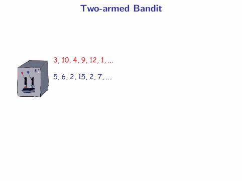
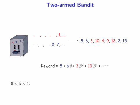
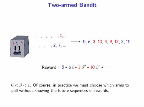
Two-armed Bandit

3, 10, 4, 9, 12, 1, ...

5, 6, 2, 15, 2, 7, ...

Two-armed Bandit

3, 10, 4, 9, 12, 1, ...

, 6, 2, 15, 2, 7, ...5

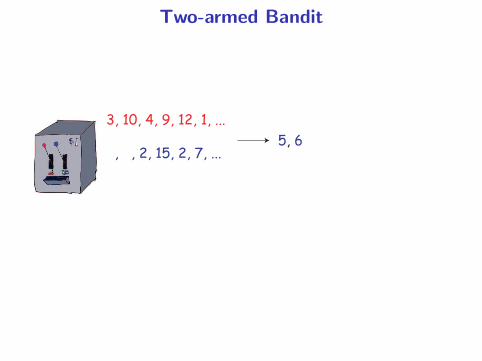
Two-armed Bandit

3, 10, 4, 9, 12, 1, ...

, , 2, 15, 2, 7, ...5, 6

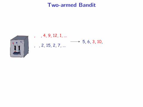
Two-armed Bandit

, 10, 4, 9, 12, 1, ...

, , 2, 15, 2, 7, ...5, 6, 3

Two-armed Bandit

, , 4, 9, 12, 1, ...

, , 2, 15, 2, 7, ...5, 6, 3, 10,

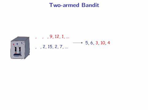
Two-armed Bandit

, , , 9, 12, 1, ...

, , 2, 15, 2, 7, ...5, 6, 3, 10, 4

Two-armed Bandit

, , , , 12, 1, ...

, , 2, 15, 2, 7, ...5, 6, 3, 10, 4, 9

Two-armed Bandit

, , , , , 1, ...

, , 2, 15, 2, 7, ...5, 6, 3, 10, 4, 9, 12

Two-armed Bandit

, , , , , 1, ...

, , , 15, 2, 7, ...5, 6, 3, 10, 4, 9, 12, 2

Two-armed Bandit

, , , , , 1, ...

, , , , 2, 7, ...5, 6, 3, 10, 4, 9, 12, 2, 15

Two-armed Bandit

, , , , , 1, ...

, , , , 2, 7, ...5, 6, 3, 10, 4, 9, 12, 2, 15

Reward = 5 + 6 + 3 + 10 + . . .β β2 β3

0 < β < 1.

Two-armed Bandit

, , , , , 1, ...

, , , , 2, 7, ...5, 6, 3, 10, 4, 9, 12, 2, 15

Reward = 5 + 6 + 3 + 10 + . . .β β2 β3

0 < β < 1. Of course, in practice we must choose which arms topull without knowing the future sequences of rewards.

Dynamic Effort Allocation

• Research projects: how should I allocate my research timeamongst my favorite open problems so as to maximize thevalue of my completed research?

Dynamic Effort Allocation

• Research projects: how should I allocate my research timeamongst my favorite open problems so as to maximize thevalue of my completed research?

• Job Scheduling: in what order should I work on the tasks inmy in-tray?

Dynamic Effort Allocation

• Research projects: how should I allocate my research timeamongst my favorite open problems so as to maximize thevalue of my completed research?

• Job Scheduling: in what order should I work on the tasks inmy in-tray?

• Searching for information: shall I spend more time browsingthe web, or go to the library, or ask a friend?

Dynamic Effort Allocation

• Research projects: how should I allocate my research timeamongst my favorite open problems so as to maximize thevalue of my completed research?

• Job Scheduling: in what order should I work on the tasks inmy in-tray?

• Searching for information: shall I spend more time browsingthe web, or go to the library, or ask a friend?

• Dating strategy: should I contact a new prospect, or tryanother date with someone I have dated before?

Information vs. Immediate Payoff

In all these problems one wishes to learn about the effectiveness ofalternative strategies, while simultaneously wishing to use the beststrategy in the short-term.

Information vs. Immediate Payoff

In all these problems one wishes to learn about the effectiveness ofalternative strategies, while simultaneously wishing to use the beststrategy in the short-term.

“Bandit problems embody in essential form a conflict

evident in all human action: information versus immediate

payoff.”

— Peter Whittle (1989)

Information vs. Immediate Payoff

In all these problems one wishes to learn about the effectiveness ofalternative strategies, while simultaneously wishing to use the beststrategy in the short-term.

“Bandit problems embody in essential form a conflict

evident in all human action: information versus immediate

payoff.”

— Peter Whittle (1989)

“Exploration versus exploitation”

Clinical Trials

Bernoulli Bandits

One of N drugs is to be administered at each of times t = 0, 1, . . .

Bernoulli Bandits

One of N drugs is to be administered at each of times t = 0, 1, . . .

The sth time drug i is used it is successful, Xi(s) = 1,or unsuccessful, Xi(s) = 0.

Bernoulli Bandits

One of N drugs is to be administered at each of times t = 0, 1, . . .

The sth time drug i is used it is successful, Xi(s) = 1,or unsuccessful, Xi(s) = 0.

P (Xi(s) = 1) = θi.

Bernoulli Bandits

One of N drugs is to be administered at each of times t = 0, 1, . . .

The sth time drug i is used it is successful, Xi(s) = 1,or unsuccessful, Xi(s) = 0.

P (Xi(s) = 1) = θi.

Xi(1),Xi(2), . . . are i.i.d. samples.

Bernoulli Bandits

One of N drugs is to be administered at each of times t = 0, 1, . . .

The sth time drug i is used it is successful, Xi(s) = 1,or unsuccessful, Xi(s) = 0.

P (Xi(s) = 1) = θi.

Xi(1),Xi(2), . . . are i.i.d. samples.

θi is unknown, but has a prior distribution,

— perhaps uniform on [0, 1]

f(θi) = 1 , 0 ≤ θi ≤ 1 .

Bernoulli Bandits

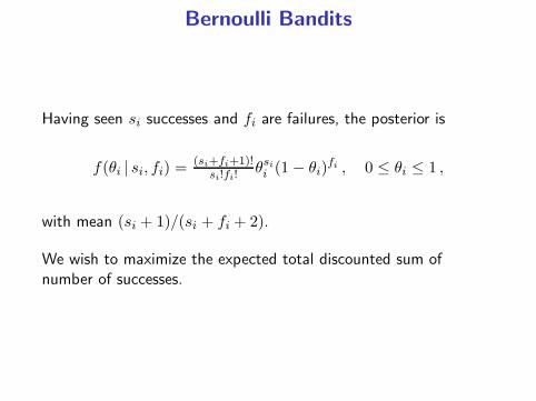
Having seen si successes and fi are failures, the posterior is

f(θi | si, fi) =(si+fi+1)!

si!fi!θsii (1− θi)

fi , 0 ≤ θi ≤ 1 ,

with mean (si + 1)/(si + fi + 2).

Bernoulli Bandits

Having seen si successes and fi are failures, the posterior is

f(θi | si, fi) =(si+fi+1)!

si!fi!θsii (1− θi)

fi , 0 ≤ θi ≤ 1 ,

with mean (si + 1)/(si + fi + 2).

We wish to maximize the expected total discounted sum ofnumber of successes.

Multi-armed Bandit

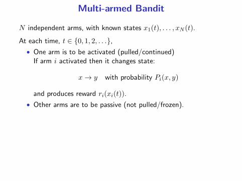
N independent arms, with known states x1(t), . . . , xN (t).

Multi-armed Bandit

N independent arms, with known states x1(t), . . . , xN (t).

At each time, t ∈ 0, 1, 2, . . .,

• One arm is to be activated (pulled/continued)If arm i activated then it changes state:

x → y with probability Pi(x, y)

and produces reward ri(xi(t)).

Multi-armed Bandit

N independent arms, with known states x1(t), . . . , xN (t).

At each time, t ∈ 0, 1, 2, . . .,

• One arm is to be activated (pulled/continued)If arm i activated then it changes state:

x → y with probability Pi(x, y)

and produces reward ri(xi(t)).

• Other arms are to be passive (not pulled/frozen).

Multi-armed Bandit

N independent arms, with known states x1(t), . . . , xN (t).

At each time, t ∈ 0, 1, 2, . . .,

• One arm is to be activated (pulled/continued)If arm i activated then it changes state:

x → y with probability Pi(x, y)

and produces reward ri(xi(t)).

• Other arms are to be passive (not pulled/frozen).

Objective: maximize the expected total β-discounted reward

E

[

∞∑

t=0

rit(xit(t))βt

]

,

where it is the arm pulled at time t, (0 < β < 1).

Dynamic Programming Solution

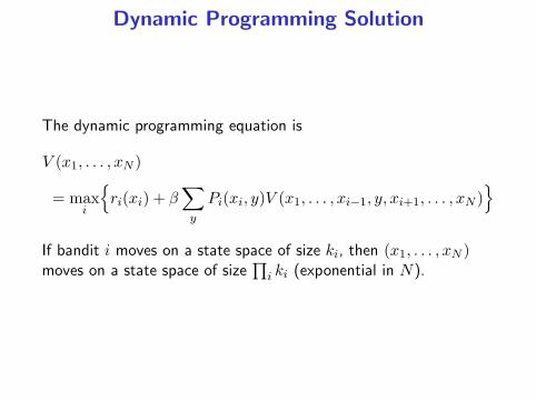
The dynamic programming equation is

V (x1, . . . , xN )

= maxi

ri(xi) + β∑

y

Pi(xi, y)V (x1, . . . , xi−1, y, xi+1, . . . , xN )

Dynamic Programming Solution

The dynamic programming equation is

V (x1, . . . , xN )

= maxi

ri(xi) + β∑

y

Pi(xi, y)V (x1, . . . , xi−1, y, xi+1, . . . , xN )

If bandit i moves on a state space of size ki, then (x1, . . . , xN )moves on a state space of size

∏

i ki (exponential in N).

Gittins Index Solution

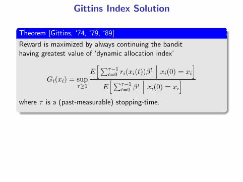
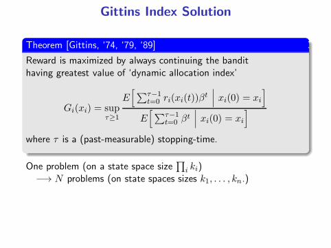
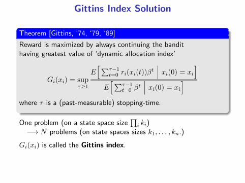
Theorem [Gittins, ‘74, ‘79, ‘89]

Reward is maximized by always continuing the bandithaving greatest value of ‘dynamic allocation index’

Gi(xi) = supτ≥1

E[

∑τ−1t=0 ri(xi(t))β

t∣

∣

∣xi(0) = xi

]

E[

∑τ−1t=0 βt

∣

∣

∣xi(0) = xi

]

where τ is a (past-measurable) stopping-time.

Gittins Index Solution

Theorem [Gittins, ‘74, ‘79, ‘89]

Reward is maximized by always continuing the bandithaving greatest value of ‘dynamic allocation index’

Gi(xi) = supτ≥1

E[

∑τ−1t=0 ri(xi(t))β

t∣

∣

∣xi(0) = xi

]

E[

∑τ−1t=0 βt

∣

∣

∣xi(0) = xi

]

where τ is a (past-measurable) stopping-time.

One problem (on a state space size∏

i ki)−→ N problems (on state spaces sizes k1, . . . , kn.)

Gittins Index Solution

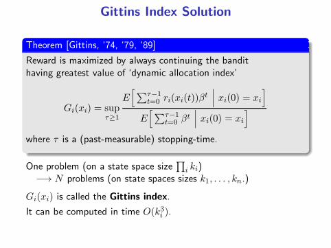
Theorem [Gittins, ‘74, ‘79, ‘89]

Reward is maximized by always continuing the bandithaving greatest value of ‘dynamic allocation index’

Gi(xi) = supτ≥1

E[

∑τ−1t=0 ri(xi(t))β

t∣

∣

∣xi(0) = xi

]

E[

∑τ−1t=0 βt

∣

∣

∣xi(0) = xi

]

where τ is a (past-measurable) stopping-time.

One problem (on a state space size∏

i ki)−→ N problems (on state spaces sizes k1, . . . , kn.)

Gi(xi) is called the Gittins index.

Gittins Index Solution

Theorem [Gittins, ‘74, ‘79, ‘89]

Reward is maximized by always continuing the bandithaving greatest value of ‘dynamic allocation index’

Gi(xi) = supτ≥1

E[

∑τ−1t=0 ri(xi(t))β

t∣

∣

∣xi(0) = xi

]

E[

∑τ−1t=0 βt

∣

∣

∣xi(0) = xi

]

where τ is a (past-measurable) stopping-time.

One problem (on a state space size∏

i ki)−→ N problems (on state spaces sizes k1, . . . , kn.)

Gi(xi) is called the Gittins index.

It can be computed in time O(k3i ).

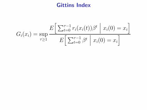
Gittins Index

Gi(xi) = supτ≥1

E[

∑τ−1t=0 ri(xi(t))β

t∣

∣

∣xi(0) = xi

]

E[

∑τ−1t=0 β

t∣

∣

∣xi(0) = xi

]

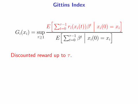
Gittins Index

Gi(xi) = supτ≥1

E[

∑τ−1t=0 ri(xi(t))β

t∣

∣

∣xi(0) = xi

]

E[

∑τ−1t=0 β

t∣

∣

∣xi(0) = xi

]

Discounted reward up to τ .

Gittins Index

Gi(xi) = supτ≥1

E[

∑τ−1t=0 ri(xi(t))β

t∣

∣

∣xi(0) = xi

]

E[

∑τ−1t=0 β

t∣

∣

∣xi(0) = xi

]

Discounted reward up to τ .

Discounted time up to τ .

Gittins Indices for Bernoulli Bandits, β = 0.9

s 2 3 4 5 6 7 8f1 .7029 .8001 .8452 .8723 .8905 .9039 .9141 .92212 .5001 .6346 .7072 .7539 .7869 .8115 .8307 .84613 .3796 .5163 .6010 .6579 .6996 .7318 .7573 .77824 .3021 .4342 .5184 .5809 .6276 .6642 .6940 .71875 .2488 .3720 .4561 .5179 .5676 .6071 .6395 .66666 .2103 .3245 .4058 .4677 .5168 .5581 .5923 .62127 .1815 .2871 .3647 .4257 .4748 .5156 .5510 .58118 .1591 .2569 .3308 .3900 .4387 .4795 .5144 .5454

(s1, f1) = (2, 3): posterior mean = 37 = 0.4286, index = 0.5163

Gittins Indices for Bernoulli Bandits, β = 0.9

s 2 3 4 5 6 7 8f1 .7029 .8001 .8452 .8723 .8905 .9039 .9141 .92212 .5001 .6346 .7072 .7539 .7869 .8115 .8307 .84613 .3796 .5163 .6010 .6579 .6996 .7318 .7573 .77824 .3021 .4342 .5184 .5809 .6276 .6642 .6940 .71875 .2488 .3720 .4561 .5179 .5676 .6071 .6395 .66666 .2103 .3245 .4058 .4677 .5168 .5581 .5923 .62127 .1815 .2871 .3647 .4257 .4748 .5156 .5510 .58118 .1591 .2569 .3308 .3900 .4387 .4795 .5144 .5454

(s1, f1) = (2, 3): posterior mean = 37 = 0.4286, index = 0.5163

(s2, f2) = (6, 7): posterior mean = 715 = 0.4667, index = 0.5156

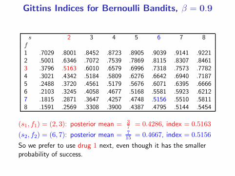
Gittins Indices for Bernoulli Bandits, β = 0.9

s 2 3 4 5 6 7 8f1 .7029 .8001 .8452 .8723 .8905 .9039 .9141 .92212 .5001 .6346 .7072 .7539 .7869 .8115 .8307 .84613 .3796 .5163 .6010 .6579 .6996 .7318 .7573 .77824 .3021 .4342 .5184 .5809 .6276 .6642 .6940 .71875 .2488 .3720 .4561 .5179 .5676 .6071 .6395 .66666 .2103 .3245 .4058 .4677 .5168 .5581 .5923 .62127 .1815 .2871 .3647 .4257 .4748 .5156 .5510 .58118 .1591 .2569 .3308 .3900 .4387 .4795 .5144 .5454

(s1, f1) = (2, 3): posterior mean = 37 = 0.4286, index = 0.5163

(s2, f2) = (6, 7): posterior mean = 715 = 0.4667, index = 0.5156

So we prefer to use drug 1 next, even though it has the smallerprobability of success.

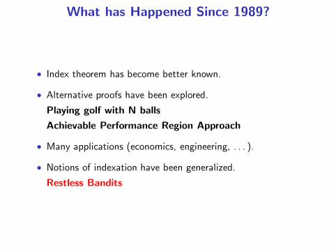
What has Happened Since 1989?

• Index theorem has become better known.

What has Happened Since 1989?

• Index theorem has become better known.

• Alternative proofs have been explored.

What has Happened Since 1989?

• Index theorem has become better known.

• Alternative proofs have been explored.

Playing golf with N balls

What has Happened Since 1989?

• Index theorem has become better known.

• Alternative proofs have been explored.

Playing golf with N balls

Achievable Performance Region Approach

What has Happened Since 1989?

• Index theorem has become better known.

• Alternative proofs have been explored.

Playing golf with N balls

Achievable Performance Region Approach

• Many applications (economics, engineering, . . . ).

What has Happened Since 1989?

• Index theorem has become better known.

• Alternative proofs have been explored.

Playing golf with N balls

Achievable Performance Region Approach

• Many applications (economics, engineering, . . . ).

• Notions of indexation have been generalized.

What has Happened Since 1989?

• Index theorem has become better known.

• Alternative proofs have been explored.

Playing golf with N balls

Achievable Performance Region Approach

• Many applications (economics, engineering, . . . ).

• Notions of indexation have been generalized.

Restless Bandits

Gittins Index Theorem

has become Better Known

Peter Whittle tells the story:

“A colleague of high repute asked an equally well-known col-league:

— What would you say if you were told that the multi-armedbandit problem had been solved?’

Gittins Index Theorem

has become Better Known

Peter Whittle tells the story:

“A colleague of high repute asked an equally well-known col-league:

— What would you say if you were told that the multi-armedbandit problem had been solved?’

— Sir, the multi-armed bandit problem is not of such anature that it can be solved.’

Proofs of the Index Theorem

Since Gittins (1974, 1979), many researchers have reproved,remodelled and resituated the index theorem.

Beale (1979)

Karatzas (1984)

Varaiya, Walrand, Buyukkoc (1985)

Chen, Katehakis (1986)

Kallenberg (1986)

Katehakis, Veinott (1986)

Eplett (1986)

Kertz (1986)

Tsitsiklis (1986)

Mandelbaum (1986, 1987)

Lai, Ying (1988)

Whittle (1988)

Proofs of the Index Theorem

Since Gittins (1974, 1979), many researchers have reproved,remodelled and resituated the index theorem.

Beale (1979)

Karatzas (1984)

Varaiya, Walrand, Buyukkoc (1985)

Chen, Katehakis (1986)

Kallenberg (1986)

Katehakis, Veinott (1986)

Eplett (1986)

Kertz (1986)

Tsitsiklis (1986)

Mandelbaum (1986, 1987)

Lai, Ying (1988)

Whittle (1988)

Weber (1992)

El Karoui, Karatzas (1993)

Ishikida and Varaiya (1994)

Tsitsiklis (1994)

Bertsimas, Nino-Mora (1996)

Glazebrook, Garbe (1996)

Kaspi, Mandelbaum (1998)

Bauerle, Stidham (2001)

Dimitriu, Tetali, Winkler (2003)

What has Happened Since 1989?

• Index theorem has become better known.

• Alternative proofs have been explored.

Playing golf with N balls

Achievable Performance Region Approach

• Many applications (economics, engineering, . . . ).

• Notions of indexation have been generalized.

Restless Bandits

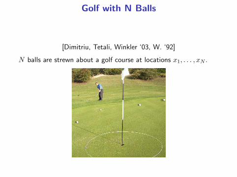
Golf with N Balls

[Dimitriu, Tetali, Winkler ‘03, W. ‘92]

N balls are strewn about a golf course at locations x1, . . . , xN .

Golf with N Balls

[Dimitriu, Tetali, Winkler ‘03, W. ‘92]

N balls are strewn about a golf course at locations x1, . . . , xN .

Hitting a ball i, that is in location xi, costs c(xi),

xi → y with probability P (xi, y)

Ball goes in the hole with probability P (xi, 0).

Objective

Minimize the expected total cost incurred up to sinking a first ball.

Golf with 1 Ball

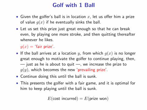
• Given the golfer’s ball is in location x, let us offer him a prizeof value g(x) if he eventually sinks the ball.

Golf with 1 Ball

• Given the golfer’s ball is in location x, let us offer him a prizeof value g(x) if he eventually sinks the ball.

• Let us set this prize just great enough so that he can breakeven, by playing one more stroke, and then quitting thereafterwhenever he likes.

Golf with 1 Ball

• Given the golfer’s ball is in location x, let us offer him a prizeof value g(x) if he eventually sinks the ball.

• Let us set this prize just great enough so that he can breakeven, by playing one more stroke, and then quitting thereafterwhenever he likes.

g(x) = ‘fair prize’.

Golf with 1 Ball

• Given the golfer’s ball is in location x, let us offer him a prizeof value g(x) if he eventually sinks the ball.

• Let us set this prize just great enough so that he can breakeven, by playing one more stroke, and then quitting thereafterwhenever he likes.

g(x) = ‘fair prize’.

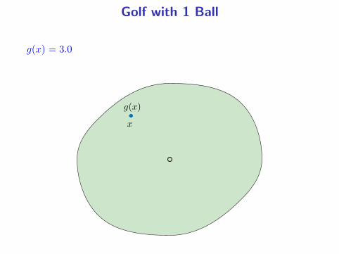
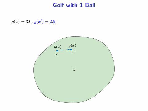
• If the ball arrives at a location y, from which g(x) is no longergreat enough to motivate the golfer to continue playing, then,— just as he is about to quit —, we increase the prize tog(y), which becomes the new ‘prevailing prize’.

Golf with 1 Ball

• Given the golfer’s ball is in location x, let us offer him a prizeof value g(x) if he eventually sinks the ball.

• Let us set this prize just great enough so that he can breakeven, by playing one more stroke, and then quitting thereafterwhenever he likes.

g(x) = ‘fair prize’.

• If the ball arrives at a location y, from which g(x) is no longergreat enough to motivate the golfer to continue playing, then,— just as he is about to quit —, we increase the prize tog(y), which becomes the new ‘prevailing prize’.

• Continue doing this until the ball is sunk.

Golf with 1 Ball

• Given the golfer’s ball is in location x, let us offer him a prizeof value g(x) if he eventually sinks the ball.

• Let us set this prize just great enough so that he can breakeven, by playing one more stroke, and then quitting thereafterwhenever he likes.

g(x) = ‘fair prize’.

• If the ball arrives at a location y, from which g(x) is no longergreat enough to motivate the golfer to continue playing, then,— just as he is about to quit —, we increase the prize tog(y), which becomes the new ‘prevailing prize’.

• Continue doing this until the ball is sunk.

• This presents the golfer with a fair game, and it is optimal forhim to keep playing until the ball is sunk.

E(cost incurred) = E(prize won)

Golf with 1 Ball

g(x) = 3.0

x

g(x)

Golf with 1 Ball

g(x) = 3.0, g(x′) = 2.5

xx′

g(x) g(x)

Golf with 1 Ball

g(x) = 3.0, g(x′) = 2.5, g(x′′) = 4.0

xx′

x′′

g(x) g(x)

g(x′′)

Golf with 1 Ball

g(x) = 3.0, g(x′) = 2.5, g(x′′) = 4.0Prevailing prize sequence is 3.0, 3.0, 4.0, . . .

xx′

x′′

g(x) g(x)

g(x′′)

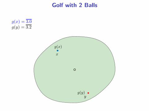
Golf with 2 Balls

g(x) = 3.0g(y) = 3.2

x

g(x)

yg(y)

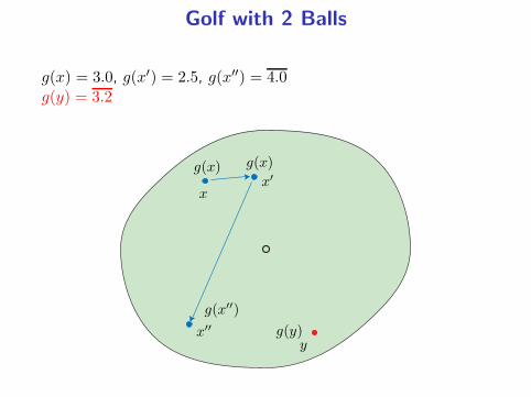
Golf with 2 Balls

g(x) = 3.0, g(x′) = 2.5g(y) = 3.2

xx′

g(x) g(x)

yg(y)

Golf with 2 Balls

g(x) = 3.0, g(x′) = 2.5, g(x′′) = 4.0g(y) = 3.2

xx′

x′′

g(x) g(x)

g(x′′)

yg(y)

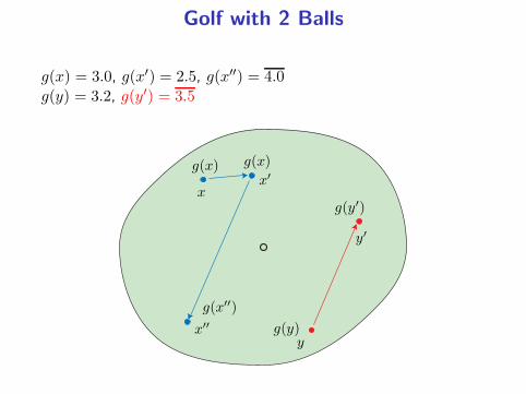
Golf with 2 Balls

g(x) = 3.0, g(x′) = 2.5, g(x′′) = 4.0g(y) = 3.2, g(y′) = 3.5

xx′

x′′

g(x) g(x)

g(x′′)

y

y′

g(y)

g(y′)

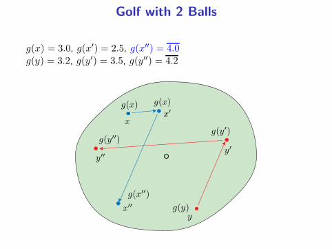
Golf with 2 Balls

g(x) = 3.0, g(x′) = 2.5, g(x′′) = 4.0g(y) = 3.2, g(y′) = 3.5, g(y′′) = 4.2

xx′

x′′

g(x) g(x)

g(x′′)

y

y′y′′

g(y)

g(y′)g(y′′)

Optimal Play with N Balls

• Each of the N balls has an initial ‘prevailing prize’, gi(0),attached to it. gi(0) = g(xi(0)).

Optimal Play with N Balls

• Each of the N balls has an initial ‘prevailing prize’, gi(0),attached to it. gi(0) = g(xi(0)).

• Prevailing prize, gi(t), is increased whenever it is insufficientto motivate golfer to play that ball; so it is nondecreasing.

Optimal Play with N Balls

• Each of the N balls has an initial ‘prevailing prize’, gi(0),attached to it. gi(0) = g(xi(0)).

• Prevailing prize, gi(t), is increased whenever it is insufficientto motivate golfer to play that ball; so it is nondecreasing.

• gi(t) depends only on the ball’s history, not what hashappened to other balls. gi(t) = maxs≤t g(xi(s)).

Optimal Play with N Balls

• Each of the N balls has an initial ‘prevailing prize’, gi(0),attached to it. gi(0) = g(xi(0)).

• Prevailing prize, gi(t), is increased whenever it is insufficientto motivate golfer to play that ball; so it is nondecreasing.

• gi(t) depends only on the ball’s history, not what hashappened to other balls. gi(t) = maxs≤t g(xi(s)).

• Game is fair. It is impossible for golfer to make a strictlypositive profit (since he would have to do so for some ball).

E(cost incurred) ≥ E(prize won)

Optimal Play with N Balls

• Each of the N balls has an initial ‘prevailing prize’, gi(0),attached to it. gi(0) = g(xi(0)).

• Prevailing prize, gi(t), is increased whenever it is insufficientto motivate golfer to play that ball; so it is nondecreasing.

• gi(t) depends only on the ball’s history, not what hashappened to other balls. gi(t) = maxs≤t g(xi(s)).

• Game is fair. It is impossible for golfer to make a strictlypositive profit (since he would have to do so for some ball).

E(cost incurred) ≥ E(prize won)

• Equality is achieved provided golfer does not switch away froma ball unless its prevailing prize increases.

Optimal Play with N Balls

• Each of the N balls has an initial ‘prevailing prize’, gi(0),attached to it. gi(0) = g(xi(0)).

• Prevailing prize, gi(t), is increased whenever it is insufficientto motivate golfer to play that ball; so it is nondecreasing.

• gi(t) depends only on the ball’s history, not what hashappened to other balls. gi(t) = maxs≤t g(xi(s)).

• Game is fair. It is impossible for golfer to make a strictlypositive profit (since he would have to do so for some ball).

E(cost incurred) ≥ E(prize won)

• Equality is achieved provided golfer does not switch away froma ball unless its prevailing prize increases.

• Right hand side is minimized by always playing ball with leastprevailing prize.

Golf and the Multi-armed Bandit

Having solved the golf problem, the solution to the multi-armedbandit problem follows. Just let P (x, 0) = 1− β for all x.

The expected cost incurred until a first ball is sunk equals theexpected total β-discounted cost over the infinite horizon.

Golf and the Multi-armed Bandit

Having solved the golf problem, the solution to the multi-armedbandit problem follows. Just let P (x, 0) = 1− β for all x.

The expected cost incurred until a first ball is sunk equals theexpected total β-discounted cost over the infinite horizon.

The fair prize, g(x), is 1/(1 − β) times the Gittins index, G(x).

Golf and the Multi-armed Bandit

Having solved the golf problem, the solution to the multi-armedbandit problem follows. Just let P (x, 0) = 1− β for all x.

The expected cost incurred until a first ball is sunk equals theexpected total β-discounted cost over the infinite horizon.

The fair prize, g(x), is 1/(1 − β) times the Gittins index, G(x).

g(x) = inf

g : supτ≥1

E

[

τ−1∑

t=0

−c(x(t))βt

+ (1− β)(1 + β + · · ·+ βτ−1)g

∣

∣

∣

∣

∣

x(0) = x

]

≥ 0

Golf and the Multi-armed Bandit

Having solved the golf problem, the solution to the multi-armedbandit problem follows. Just let P (x, 0) = 1− β for all x.

The expected cost incurred until a first ball is sunk equals theexpected total β-discounted cost over the infinite horizon.

The fair prize, g(x), is 1/(1 − β) times the Gittins index, G(x).

g(x) = inf

g : supτ≥1

E

[

τ−1∑

t=0

−c(x(t))βt

+ (1− β)(1 + β + · · ·+ βτ−1)g

∣

∣

∣

∣

∣

x(0) = x

]

≥ 0

=1

1− βinfτ≥1

E[

∑τ−1t=0 c(x(t))βt

∣

∣

∣x(0) = x

]

E[

∑τ−1t=0 βt

∣

∣

∣x(0) = x

]

Golf with N Balls and a Set of Clubs

Suppose that a ball in location x can be played with a choice ofshots, from a set A(x). Choosing shot a ∈ A(x),

x → y with probability Pa(x, y)

Now the golfer must choose, not only which ball to play, but withwhich shot to play it.

Golf with N Balls and a Set of Clubs

Suppose that a ball in location x can be played with a choice ofshots, from a set A(x). Choosing shot a ∈ A(x),

x → y with probability Pa(x, y)

Now the golfer must choose, not only which ball to play, but withwhich shot to play it.

Under a condition, an index policy is again optimal.

He should play the ball with least prevailing prize, choosing theshot from A that is optimal if that ball were the only ball present.

What has Happened Since 1989?

• Index theorem has become better known.

• Alternative proofs have been explored.

Playing golf with N balls

Achievable Performance Region Approach

• Many applications (economics, engineering, . . . ).

• Notions of indexation have been generalized.

Restless Bandits

Achievable Performance Region Approach

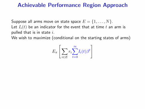
Suppose all arms move on state space E = 1, . . . , N.Let Ii(t) be an indicator for the event that at time t an arm ispulled that is in state i.We wish to maximize (conditional on the starting states of arms)

Eπ

[

∑

i∈E

ri

∞∑

t=0

Ii(t)βt

]

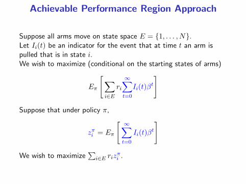
Achievable Performance Region Approach

Suppose all arms move on state space E = 1, . . . , N.Let Ii(t) be an indicator for the event that at time t an arm ispulled that is in state i.We wish to maximize (conditional on the starting states of arms)

Eπ

[

∑

i∈E

ri

∞∑

t=0

Ii(t)βt

]

Suppose that under policy π,

zπi = Eπ

[

∞∑

t=0

Ii(t)βt

]

We wish to maximize∑

i∈E rizπi .

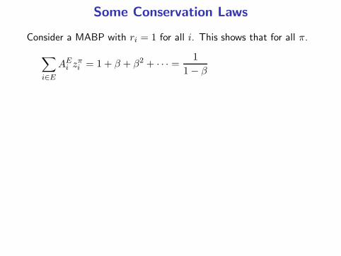
Some Conservation Laws

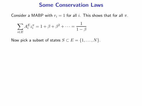
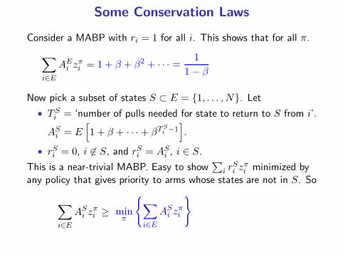
Consider a MABP with ri = 1 for all i. This shows that for all π.

∑

i∈E

zπi = 1 + β + β2 + · · · =1

1− β

Some Conservation Laws

Consider a MABP with ri = 1 for all i. This shows that for all π.

∑

i∈E

AEi z

πi = 1 + β + β2 + · · · =

1

1− β

Some Conservation Laws

Consider a MABP with ri = 1 for all i. This shows that for all π.

∑

i∈E

AEi z

πi = 1 + β + β2 + · · · =

1

1− β

Now pick a subset of states S ⊂ E = 1, . . . , N.

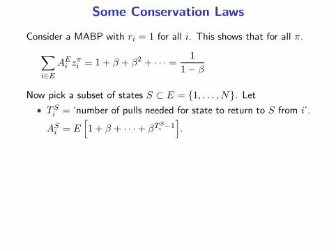
Some Conservation Laws

Consider a MABP with ri = 1 for all i. This shows that for all π.

∑

i∈E

AEi z

πi = 1 + β + β2 + · · · =

1

1− β

Now pick a subset of states S ⊂ E = 1, . . . , N. Let

• T Si = ‘number of pulls needed for state to return to S from i’.

ASi = E

[

1 + β + · · ·+ βTSi −1

]

.

Some Conservation Laws

Consider a MABP with ri = 1 for all i. This shows that for all π.

∑

i∈E

AEi z

πi = 1 + β + β2 + · · · =

1

1− β

Now pick a subset of states S ⊂ E = 1, . . . , N. Let

• T Si = ‘number of pulls needed for state to return to S from i’.

ASi = E

[

1 + β + · · ·+ βTSi −1

]

.

• rSi = 0, i 6∈ S, and rSi = ASi , i ∈ S.

Some Conservation Laws

Consider a MABP with ri = 1 for all i. This shows that for all π.

∑

i∈E

AEi z

πi = 1 + β + β2 + · · · =

1

1− β

Now pick a subset of states S ⊂ E = 1, . . . , N. Let

• T Si = ‘number of pulls needed for state to return to S from i’.

ASi = E

[

1 + β + · · ·+ βTSi −1

]

.

• rSi = 0, i 6∈ S, and rSi = ASi , i ∈ S.

This is a near-trivial MABP. Easy to show∑

i rSi z

πi minimized by

any policy that gives priority to arms whose states are not in S. So

∑

i∈E

ASi z

πi ≥ min

π

∑

i∈E

ASi z

πi

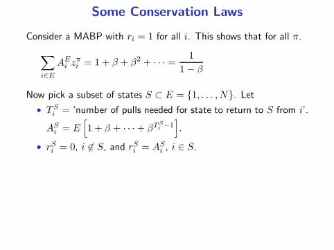
Some Conservation Laws

Consider a MABP with ri = 1 for all i. This shows that for all π.

∑

i∈E

AEi z

πi = 1 + β + β2 + · · · =

1

1− β

Now pick a subset of states S ⊂ E = 1, . . . , N. Let

• T Si = ‘number of pulls needed for state to return to S from i’.

ASi = E

[

1 + β + · · ·+ βTSi −1

]

.

• rSi = 0, i 6∈ S, and rSi = ASi , i ∈ S.

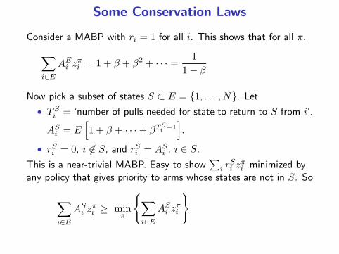
This is a near-trivial MABP. Easy to show∑

i rSi z

πi minimized by

any policy that gives priority to arms whose states are not in S. So

∑

i∈E

ASi z

πi ≥ min

π

∑

i∈E

ASi z

πi

Some Conservation Laws

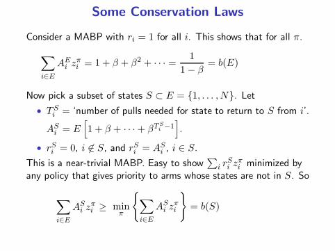
Consider a MABP with ri = 1 for all i. This shows that for all π.

∑

i∈E

AEi z

πi = 1 + β + β2 + · · · =

1

1− β= b(E)

Now pick a subset of states S ⊂ E = 1, . . . , N. Let

• T Si = ‘number of pulls needed for state to return to S from i’.

ASi = E

[

1 + β + · · ·+ βTSi −1

]

.

• rSi = 0, i 6∈ S, and rSi = ASi , i ∈ S.

This is a near-trivial MABP. Easy to show∑

i rSi z

πi minimized by

any policy that gives priority to arms whose states are not in S. So

∑

i∈E

ASi z

πi ≥ min

π

∑

i∈E

ASi z

πi

= b(S)

Constraints on the Achieveable Region

Lemma

There exist positive ASi , as defined above, such that for any schedul-

ing policy π,

∑

i∈S

ASi z

πi ≥ b(S) , for all S ⊂ E, (1)

∑

i∈E

AEi z

πi = b(E) , (2)

and such that equality holds in (1) if π gives priority to arms whosestates are not in S over any arms whose states are in S.

A Linear Programming Relaxation

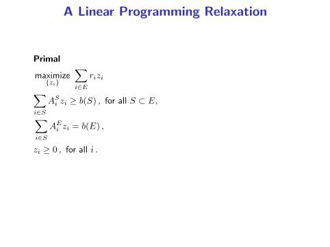
Primal

maximizezi

∑

i∈E

rizi

∑

i∈S

ASi zi ≥ b(S) , for all S ⊂ E,

∑

i∈S

AEi zi = b(E) ,

zi ≥ 0 , for all i .

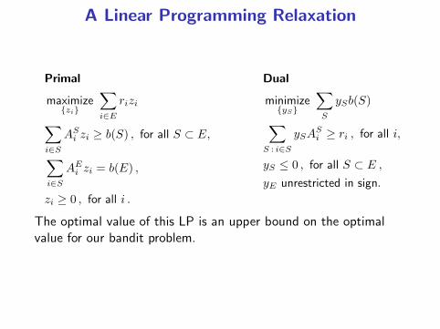
A Linear Programming Relaxation

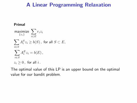
Primal

maximizezi

∑

i∈E

rizi

∑

i∈S

ASi zi ≥ b(S) , for all S ⊂ E,

∑

i∈S

AEi zi = b(E) ,

zi ≥ 0 , for all i .

The optimal value of this LP is an upper bound on the optimalvalue for our bandit problem.

A Linear Programming Relaxation

Primal

maximizezi

∑

i∈E

rizi

∑

i∈S

ASi zi ≥ b(S) , for all S ⊂ E,

∑

i∈S

AEi zi = b(E) ,

zi ≥ 0 , for all i .

Dual

minimizeyS

∑

S

ySb(S)

∑

S : i∈S

ySASi ≥ ri , for all i,

yS ≤ 0 , for all S ⊂ E ,

yE unrestricted in sign.

The optimal value of this LP is an upper bound on the optimalvalue for our bandit problem.

A Linear Programming Relaxation

Primal

maximizezi

∑

i∈E

rizi

∑

i∈S

ASi zi ≥ b(S) , for all S ⊂ E,

∑

i∈S

AEi zi = b(E) ,

zi ≥ 0 , for all i .

Dual

minimizeyS

∑

S

ySb(S)

∑

S : i∈S

ySASi ≥ ri , for all i,

yS ≤ 0 , for all S ⊂ E ,

yE unrestricted in sign.

The optimal value of this LP is an upper bound on the optimalvalue for our bandit problem.

A greedy algorithm computes dual vectors yS that are dual feasibleand complementary slack, and a primal solution zi = zπi which isthe performance vector of a priority policy.

A Linear Programming Relaxation

Primal

maximizezi

∑

i∈E

rizi

∑

i∈S

ASi zi ≥ b(S) , for all S ⊂ E,

∑

i∈S

AEi zi = b(E) ,

zi ≥ 0 , for all i .

Dual

minimizeyS

∑

S

ySb(S)

∑

S : i∈S

ySASi ≥ ri , for all i,

yS ≤ 0 , for all S ⊂ E ,

yE unrestricted in sign.

The optimal value of this LP is an upper bound on the optimalvalue for our bandit problem.

A greedy algorithm computes dual vectors yS that are dual feasibleand complementary slack, and a primal solution zi = zπi which isthe performance vector of a priority policy.

A Linear Programming Relaxation

Primal

maximizezi

∑

i∈E

rizi

∑

i∈S

ASi zi ≥ b(S) , for all S ⊂ E,

∑

i∈S

AEi zi = b(E) ,

zi ≥ 0 , for all i .

Dual

minimizeyS

∑

S

ySb(S)

∑

S : i∈S

ySASi ≥ ri , for all i,

yS ≤ 0 , for all S ⊂ E ,

yE unrestricted in sign.

The optimal value of this LP is an upper bound on the optimalvalue for our bandit problem.

A greedy algorithm computes dual vectors yS that are dual feasibleand complementary slack, and a primal solution zi = zπi which isthe performance vector of a priority policy.

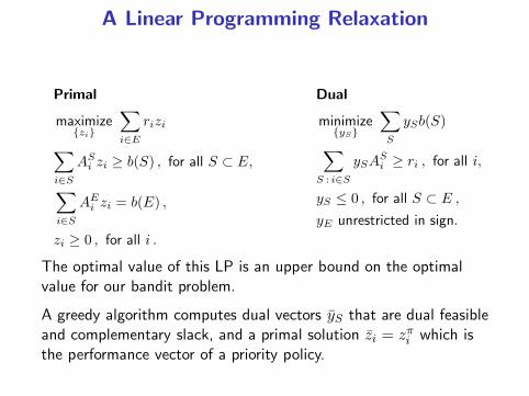
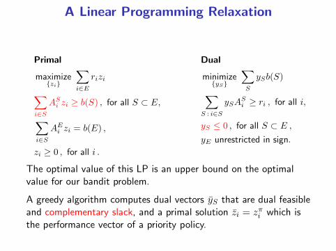
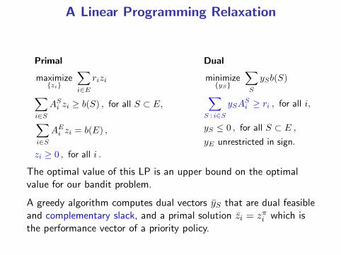
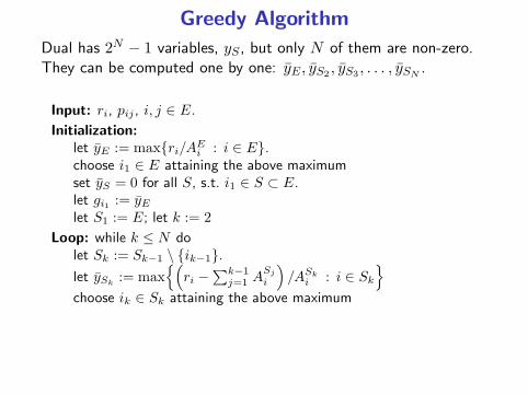
Greedy Algorithm

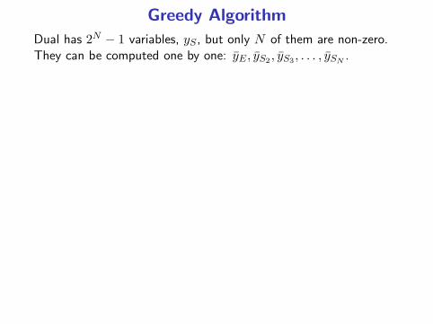
Dual has 2N − 1 variables, yS, but only N of them are non-zero.They can be computed one by one: yE, yS2

, yS3, . . . , ySN

.

Greedy Algorithm

Dual has 2N − 1 variables, yS, but only N of them are non-zero.They can be computed one by one: yE, yS2

, yS3, . . . , ySN

.

Input: ri, pij , i, j ∈ E.

Initialization:

let yE := maxri/AEi : i ∈ E.

Greedy Algorithm

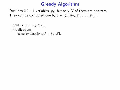
Dual has 2N − 1 variables, yS, but only N of them are non-zero.They can be computed one by one: yE, yS2

, yS3, . . . , ySN

.

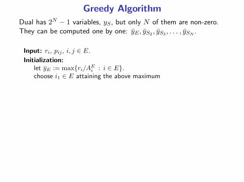
Input: ri, pij , i, j ∈ E.

Initialization:

let yE := maxri/AEi : i ∈ E.

choose i1 ∈ E attaining the above maximum

Greedy Algorithm

Dual has 2N − 1 variables, yS, but only N of them are non-zero.They can be computed one by one: yE, yS2

, yS3, . . . , ySN

.

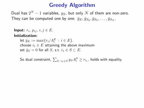
Input: ri, pij , i, j ∈ E.

Initialization:

let yE := maxri/AEi : i ∈ E.

choose i1 ∈ E attaining the above maximumset yS = 0 for all S, s.t. i1 ∈ S ⊂ E.

So dual constraint,∑

S : i1∈S ySASi ≥ ri1 , holds with equality.

Greedy Algorithm

Dual has 2N − 1 variables, yS, but only N of them are non-zero.They can be computed one by one: yE, yS2

, yS3, . . . , ySN

.

Input: ri, pij , i, j ∈ E.

Initialization:

let yE := maxri/AEi : i ∈ E.

choose i1 ∈ E attaining the above maximumset yS = 0 for all S, s.t. i1 ∈ S ⊂ E.let gi1 := yElet S1 := E; let k := 2

Greedy Algorithm

Dual has 2N − 1 variables, yS, but only N of them are non-zero.They can be computed one by one: yE, yS2

, yS3, . . . , ySN

.

Input: ri, pij , i, j ∈ E.

Initialization:

let yE := maxri/AEi : i ∈ E.

choose i1 ∈ E attaining the above maximumset yS = 0 for all S, s.t. i1 ∈ S ⊂ E.let gi1 := yElet S1 := E; let k := 2

Loop: while k ≤ N dolet Sk := Sk−1 \ ik−1.

let ySk:= max

(

ri −∑k−1

j=1A

Sj

i

)

/ASk

i : i ∈ Sk

choose ik ∈ Sk attaining the above maximum

Greedy Algorithm

Dual has 2N − 1 variables, yS, but only N of them are non-zero.They can be computed one by one: yE, yS2

, yS3, . . . , ySN

.

Input: ri, pij , i, j ∈ E.

Initialization:

let yE := maxri/AEi : i ∈ E.

choose i1 ∈ E attaining the above maximumset yS = 0 for all S, s.t. i1 ∈ S ⊂ E.let gi1 := yElet S1 := E; let k := 2

Loop: while k ≤ N dolet Sk := Sk−1 \ ik−1.

let ySk:= max

(

ri −∑k−1

j=1A

Sj

i

)

/ASk

i : i ∈ Sk

choose ik ∈ Sk attaining the above maximumset yS = 0 for all S, s.t. ik ∈ S ⊂ Sk.

So dual constraint,∑

S : ik∈S ySASi ≥ rik , holds with equality.

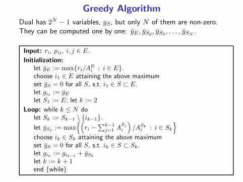
Greedy Algorithm

Dual has 2N − 1 variables, yS, but only N of them are non-zero.They can be computed one by one: yE, yS2

, yS3, . . . , ySN

.

Input: ri, pij , i, j ∈ E.

Initialization:

let yE := maxri/AEi : i ∈ E.

choose i1 ∈ E attaining the above maximumset yS = 0 for all S, s.t. i1 ∈ S ⊂ E.let gi1 := yElet S1 := E; let k := 2

Loop: while k ≤ N dolet Sk := Sk−1 \ ik−1.

let ySk:= max

(

ri −∑k−1

j=1A

Sj

i

)

/ASk

i : i ∈ Sk

choose ik ∈ Sk attaining the above maximumset yS = 0 for all S, s.t. ik ∈ S ⊂ Sk.let gik := gik−1

+ ySk

let k := k + 1end while

What has Happened Since 1989?

• Index theorem has become better known.

• Alternative proofs have been explored.

Playing golf with N balls

Achievable Performance Region Approach

• Many applications (economics, engineering, . . . ).

• Notions of indexation have been generalized.

Restless Bandits

Restless Bandits

Spinning Plates

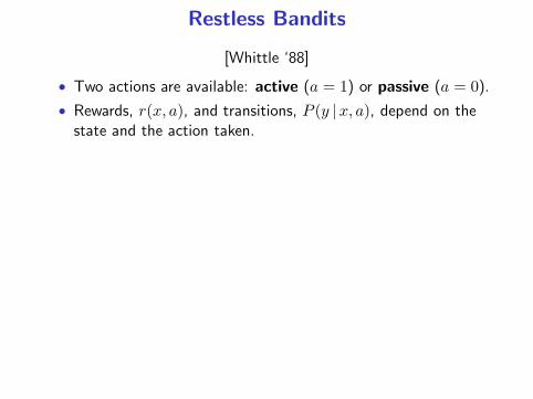
Restless Bandits

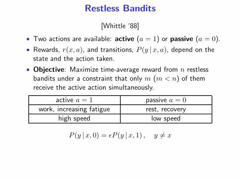
[Whittle ‘88]

• Two actions are available: active (a = 1) or passive (a = 0).

Restless Bandits

[Whittle ‘88]

• Two actions are available: active (a = 1) or passive (a = 0).

• Rewards, r(x, a), and transitions, P (y |x, a), depend on thestate and the action taken.

Restless Bandits

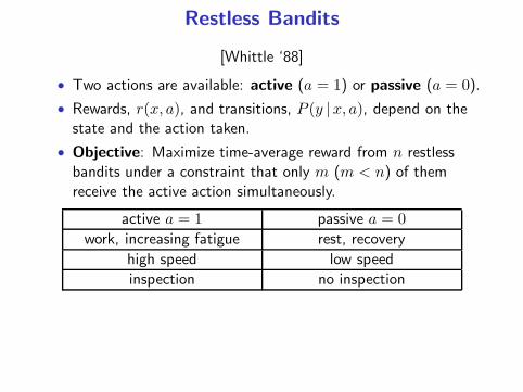
[Whittle ‘88]

• Two actions are available: active (a = 1) or passive (a = 0).

• Rewards, r(x, a), and transitions, P (y |x, a), depend on thestate and the action taken.

• Objective: Maximize time-average reward from n restlessbandits under a constraint that only m (m < n) of themreceive the active action simultaneously.

Restless Bandits

[Whittle ‘88]

• Two actions are available: active (a = 1) or passive (a = 0).

• Rewards, r(x, a), and transitions, P (y |x, a), depend on thestate and the action taken.

• Objective: Maximize time-average reward from n restlessbandits under a constraint that only m (m < n) of themreceive the active action simultaneously.

active a = 1 passive a = 0

work, increasing fatigue rest, recovery

Restless Bandits

[Whittle ‘88]

• Two actions are available: active (a = 1) or passive (a = 0).

• Rewards, r(x, a), and transitions, P (y |x, a), depend on thestate and the action taken.

• Objective: Maximize time-average reward from n restlessbandits under a constraint that only m (m < n) of themreceive the active action simultaneously.

active a = 1 passive a = 0

work, increasing fatigue rest, recovery

high speed low speed

P (y |x, 0) = εP (y |x, 1) , y 6= x

Restless Bandits

[Whittle ‘88]

• Two actions are available: active (a = 1) or passive (a = 0).

• Rewards, r(x, a), and transitions, P (y |x, a), depend on thestate and the action taken.

• Objective: Maximize time-average reward from n restlessbandits under a constraint that only m (m < n) of themreceive the active action simultaneously.

active a = 1 passive a = 0

work, increasing fatigue rest, recovery

high speed low speed

inspection no inspection

Opportunistic Spectrum Access

Communication channels may be busy or free.

0 1 2 3 T

Channel 1

Channel 2

Opportunities

Opportunities

Opportunistic Spectrum Access

Communication channels may be busy or free.

0 1 2 3 T

Channel 1

Channel 2

Opportunities

Opportunities

Aim is to ‘inspect’ m out of n channels, maximizing the number ofthese that are found to be free.

Opportunistic Spectrum Access

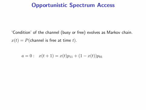
‘Condition’ of the channel (busy or free) evolves as Markov chain.

x(t) = P (channel is free at time t).

Opportunistic Spectrum Access

‘Condition’ of the channel (busy or free) evolves as Markov chain.

x(t) = P (channel is free at time t).

a = 0 : x(t+ 1) = x(t)p11 + (1− x(t))p01

Opportunistic Spectrum Access

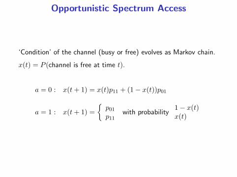
‘Condition’ of the channel (busy or free) evolves as Markov chain.

x(t) = P (channel is free at time t).

a = 0 : x(t+ 1) = x(t)p11 + (1− x(t))p01

a = 1 : x(t+ 1) =

p01p11

with probability1− x(t)x(t)

Dynamic Programming Equation

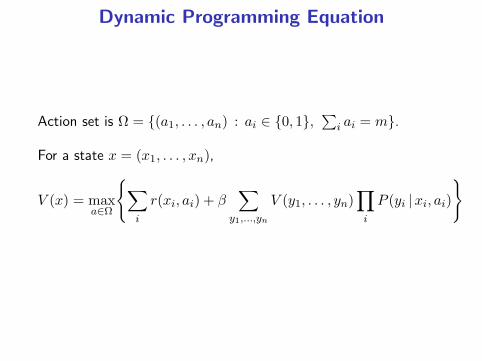
Action set is Ω = (a1, . . . , an) : ai ∈ 0, 1,∑

i ai = m.

For a state x = (x1, . . . , xn),

V (x) = maxa∈Ω

∑

i

r(xi, ai) + β∑

y1,...,yn

V (y1, . . . , yn)∏

i

P (yi |xi, ai)

Relaxed Problem for a Single Restless Bandit

Let us consider a relaxed problem, posed for 1 bandit only.

The aim is to maximize average reward obtained from this banditunder a constraint that a = 1 for only a fraction m/n of the time.

LP for the Relaxed Problem

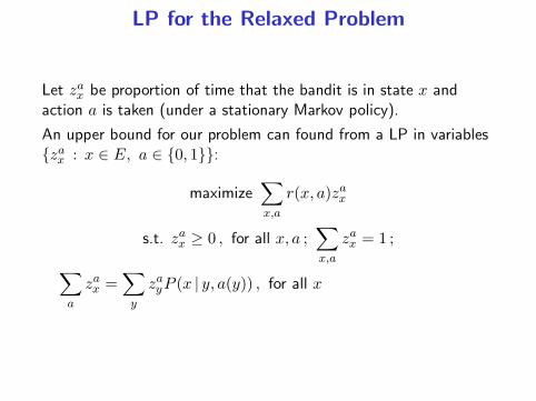
Let zax be proportion of time that the bandit is in state x andaction a is taken (under a stationary Markov policy).

An upper bound for our problem can found from a LP in variableszax : x ∈ E, a ∈ 0, 1:

maximize∑

x,a

r(x, a)zax

LP for the Relaxed Problem

Let zax be proportion of time that the bandit is in state x andaction a is taken (under a stationary Markov policy).

An upper bound for our problem can found from a LP in variableszax : x ∈ E, a ∈ 0, 1:

maximize∑

x,a

r(x, a)zax

s.t. zax ≥ 0 , for all x, a

LP for the Relaxed Problem

Let zax be proportion of time that the bandit is in state x andaction a is taken (under a stationary Markov policy).

An upper bound for our problem can found from a LP in variableszax : x ∈ E, a ∈ 0, 1:

maximize∑

x,a

r(x, a)zax

s.t. zax ≥ 0 , for all x, a ;∑

x,a

zax = 1

LP for the Relaxed Problem

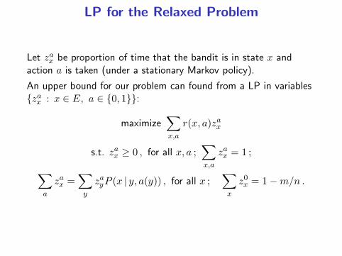
Let zax be proportion of time that the bandit is in state x andaction a is taken (under a stationary Markov policy).

An upper bound for our problem can found from a LP in variableszax : x ∈ E, a ∈ 0, 1:

maximize∑

x,a

r(x, a)zax

s.t. zax ≥ 0 , for all x, a ;∑

x,a

zax = 1 ;

∑

a

zax =∑

y

zayP (x | y, a(y)) , for all x

LP for the Relaxed Problem

Let zax be proportion of time that the bandit is in state x andaction a is taken (under a stationary Markov policy).

An upper bound for our problem can found from a LP in variableszax : x ∈ E, a ∈ 0, 1:

maximize∑

x,a

r(x, a)zax

s.t. zax ≥ 0 , for all x, a ;∑

x,a

zax = 1 ;

∑

a

zax =∑

y

zayP (x | y, a(y)) , for all x ;∑

x

z0x = 1−m/n .

The Subsidy Problem

Optimal value of the dual LP problem is g, where this can befound from the average-cost dynamic programming equation

φ(x) + g = maxa∈0,1

r(x, a) + λ(1− a) +∑

y

φ(y)P (y |x, a)

.

λ and φ(x) are the Lagrange multipliers for constraints.

λ may be interpreted as a subsidy for taking a = 0.

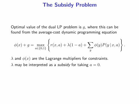
The Subsidy Problem

Optimal value of the dual LP problem is g, where this can befound from the average-cost dynamic programming equation

φ(x) + g = maxa∈0,1

r(x, a) + λ(1− a) +∑

y

φ(y)P (y |x, a)

.

λ and φ(x) are the Lagrange multipliers for constraints.

λ may be interpreted as a subsidy for taking a = 0.

Solution partitions state space into sets: E0 (a = 0), E1 (a = 1)and E01 (randomization between a = 0 and a = 1).

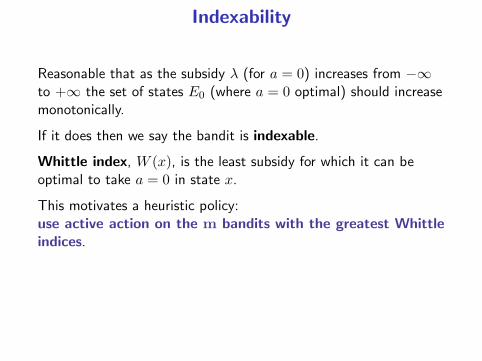
Indexability

Reasonable that as the subsidy λ (for a = 0) increases from −∞to +∞ the set of states E0 (where a = 0 optimal) should increasemonotonically.

If it does then we say the bandit is indexable.

Indexability

Reasonable that as the subsidy λ (for a = 0) increases from −∞to +∞ the set of states E0 (where a = 0 optimal) should increasemonotonically.

If it does then we say the bandit is indexable.

Whittle index, W (x), is the least subsidy for which it can beoptimal to take a = 0 in state x.

Indexability

Reasonable that as the subsidy λ (for a = 0) increases from −∞to +∞ the set of states E0 (where a = 0 optimal) should increasemonotonically.

If it does then we say the bandit is indexable.

Whittle index, W (x), is the least subsidy for which it can beoptimal to take a = 0 in state x.

This motivates a heuristic policy:use active action on the m bandits with the greatest Whittle

indices.

Indexability

Reasonable that as the subsidy λ (for a = 0) increases from −∞to +∞ the set of states E0 (where a = 0 optimal) should increasemonotonically.

If it does then we say the bandit is indexable.

Whittle index, W (x), is the least subsidy for which it can beoptimal to take a = 0 in state x.

This motivates a heuristic policy:use active action on the m bandits with the greatest Whittle

indices.

Like Gittins indices for classical bandits, Whittle indices can becomputed separately for each bandit.Same as the Gittins index when a = 0 is freezing action.

Two Questions

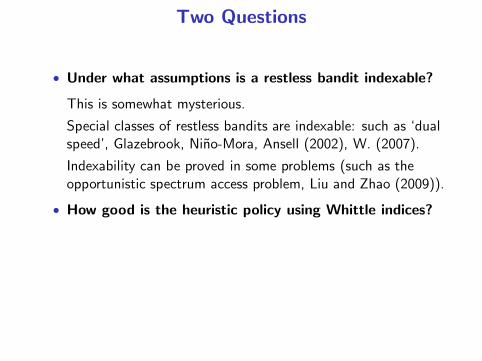
• Under what assumptions is a restless bandit indexable?

Two Questions

• Under what assumptions is a restless bandit indexable?

This is somewhat mysterious.

Special classes of restless bandits are indexable: such as ‘dualspeed’, Glazebrook, Nino-Mora, Ansell (2002), W. (2007).

Two Questions

• Under what assumptions is a restless bandit indexable?

This is somewhat mysterious.

Special classes of restless bandits are indexable: such as ‘dualspeed’, Glazebrook, Nino-Mora, Ansell (2002), W. (2007).

Indexability can be proved in some problems (such as theopportunistic spectrum access problem, Liu and Zhao (2009)).

Two Questions

• Under what assumptions is a restless bandit indexable?

This is somewhat mysterious.

Special classes of restless bandits are indexable: such as ‘dualspeed’, Glazebrook, Nino-Mora, Ansell (2002), W. (2007).

Indexability can be proved in some problems (such as theopportunistic spectrum access problem, Liu and Zhao (2009)).

• How good is the heuristic policy using Whittle indices?

Two Questions

• Under what assumptions is a restless bandit indexable?

This is somewhat mysterious.

Special classes of restless bandits are indexable: such as ‘dualspeed’, Glazebrook, Nino-Mora, Ansell (2002), W. (2007).

Indexability can be proved in some problems (such as theopportunistic spectrum access problem, Liu and Zhao (2009)).

• How good is the heuristic policy using Whittle indices?

It may be optimal. (opportunistic spectrum access —identical channels, Ahmad, Liu, Javidi, and Zhao (2009)).

Two Questions

• Under what assumptions is a restless bandit indexable?

This is somewhat mysterious.

Special classes of restless bandits are indexable: such as ‘dualspeed’, Glazebrook, Nino-Mora, Ansell (2002), W. (2007).

Indexability can be proved in some problems (such as theopportunistic spectrum access problem, Liu and Zhao (2009)).

• How good is the heuristic policy using Whittle indices?

It may be optimal. (opportunistic spectrum access —identical channels, Ahmad, Liu, Javidi, and Zhao (2009)).

Lots of papers with numerical work.

Two Questions

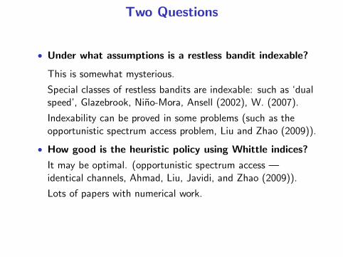
• Under what assumptions is a restless bandit indexable?

This is somewhat mysterious.

Special classes of restless bandits are indexable: such as ‘dualspeed’, Glazebrook, Nino-Mora, Ansell (2002), W. (2007).

Indexability can be proved in some problems (such as theopportunistic spectrum access problem, Liu and Zhao (2009)).

• How good is the heuristic policy using Whittle indices?

It may be optimal. (opportunistic spectrum access —identical channels, Ahmad, Liu, Javidi, and Zhao (2009)).

Lots of papers with numerical work.

It is often asymptotically optimal, W. and Weiss (1990).

Asymptotic Optimality

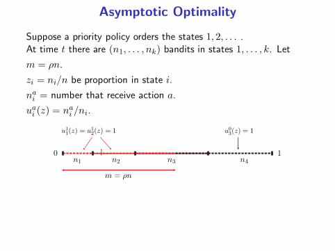
Suppose a priority policy orders the states 1, 2, . . . .At time t there are (n1, . . . , nk) bandits in states 1, . . . , k. Let

m = ρn.

Asymptotic Optimality

Suppose a priority policy orders the states 1, 2, . . . .At time t there are (n1, . . . , nk) bandits in states 1, . . . , k. Let

m = ρn.

zi = ni/n be proportion in state i.

Asymptotic Optimality

Suppose a priority policy orders the states 1, 2, . . . .At time t there are (n1, . . . , nk) bandits in states 1, . . . , k. Let

m = ρn.

zi = ni/n be proportion in state i.

nai = number that receive action a.

Asymptotic Optimality

Suppose a priority policy orders the states 1, 2, . . . .At time t there are (n1, . . . , nk) bandits in states 1, . . . , k. Let

m = ρn.

zi = ni/n be proportion in state i.

nai = number that receive action a.

uai (z) = nai /ni.

Asymptotic Optimality

Suppose a priority policy orders the states 1, 2, . . . .At time t there are (n1, . . . , nk) bandits in states 1, . . . , k. Let

m = ρn.

zi = ni/n be proportion in state i.

nai = number that receive action a.

uai (z) = nai /ni.

n1 n2 n3 n4

m = ρn

0 1

u11(z) = u12(z) = 1 u03(z) = 1

Asymptotic Optimality

Suppose a priority policy orders the states 1, 2, . . . .At time t there are (n1, . . . , nk) bandits in states 1, . . . , k. Let

m = ρn.

zi = ni/n be proportion in state i.

nai = number that receive action a.

uai (z) = nai /ni.

n1 n2 n3 n4

m = ρn

0 1

u11(z) = u12(z) = 1 0 < u13(z) < 1 u03(z) = 1

Asymptotic Optimality

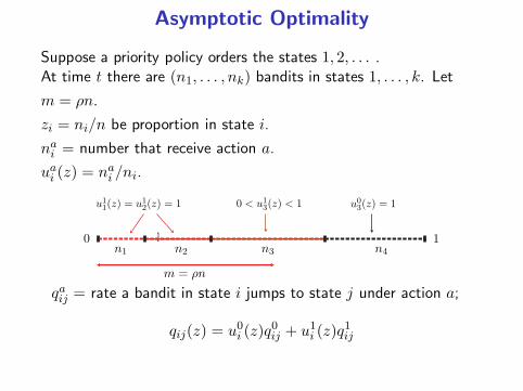
Suppose a priority policy orders the states 1, 2, . . . .At time t there are (n1, . . . , nk) bandits in states 1, . . . , k. Let

m = ρn.

zi = ni/n be proportion in state i.

nai = number that receive action a.

uai (z) = nai /ni.

n1 n2 n3 n4

m = ρn

0 1

u11(z) = u12(z) = 1 0 < u13(z) < 1 u03(z) = 1

qaij = rate a bandit in state i jumps to state j under action a;

qij(z) = u0i (z)q0ij + u1i (z)q

1ij

Fluid Approximation

The ‘fluid approximation’ for large n is given by piecewise lineardifferential equations, of the form:

dzi/dt =∑

j

qji(z)zj −∑

j

qij(z)zi

E.g., k = 2.

dz1/dt =

−(q012 + q021)z1 + (q012 − q112)ρ+ q021 , z1 ≥ ρ

−(q112 + q121)z1 − (q021 − q121)ρ+ q021 , z1 ≤ ρ

Fluid Approximation

The ‘fluid approximation’ for large n is given by piecewise lineardifferential equations, of the form:

dzi/dt =∑

j

qji(z)zj −∑

j

qij(z)zi

E.g., k = 2.

dz1/dt =

−(q012 + q021)z1 + (q012 − q112)ρ+ q021 , z1 ≥ ρ

−(q112 + q121)z1 − (q021 − q121)ρ+ q021 , z1 ≤ ρ

dz/dt = A(z)z + b(z), where A(z) and b(z) are constant within kpolyhedral regions.

Asymptotic Optimality

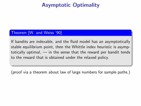
Theorem [W. and Weiss ‘90]

If bandits are indexable, and the fluid model has an asymptoticallystable equilibrium point, then the Whittle index heuristic is asymp-totically optimal, — in the sense that the reward per bandit tendsto the reward that is obtained under the relaxed policy.

(proof via a theorem about law of large numbers for sample paths.)

Heuristic May Not be Asymptotically Optimal

(

q0ij

)

=

−2 1 0 12 −2 0 00 56 − 113

2

1

2

1 1 1

2− 5

2

,(

q1ij

)

=

−2 1 0 12 −2 0 00 7

25− 113

400

1

400

1 1 1

2− 5

2

r0 = (0, 1, 10, 10) , r1 = (10, 10, 10, 0) , ρ = 0.835

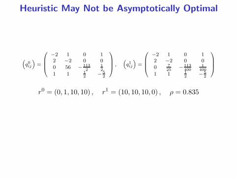
Heuristic May Not be Asymptotically Optimal

(

q0ij

)

=

−2 1 0 12 −2 0 00 56 − 113

2

1

2

1 1 1

2− 5

2

,(

q1ij

)

=

−2 1 0 12 −2 0 00 7

25− 113

400

1

400

1 1 1

2− 5

2

r0 = (0, 1, 10, 10) , r1 = (10, 10, 10, 0) , ρ = 0.835

Bandit is indexable.

Equilibrium point is (z1, z2, z3, z4) = (0.409, 0.327, 0.100, 0.164).

z1 + z2 + z3 = 0.836.

Relaxed policy obtains 10 per bandit per unit time.

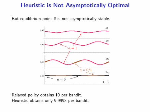
Heuristic is Not Asymptotically Optimal

But equilibrium point z is not asymptotically stable.

0.10

0.16

0.32

0.42

z1

z2

z3

z4

t →

a = 1

a = 0

a = 0/1

Relaxed policy obtains 10 per bandit.Heuristic obtains only 9.9993 per bandit.

Questions