Embed Size (px)
Citation preview

6th 13th ERCOFTAC/IAHR Workshop on Refined Turbulence Modelling, September 25-26, 2008, TU Graz, Austria
Test Case 2: 3D Diffuser
Muhamed Hadžiabdic
International University of Sarajevo, Faculty of Natural Sciences and Engineering
Paromlinska 66, 71 000 Sarajevo, Bosnia and Herzegovina
Introduction
The 3D diffuser that was experimentally investigated by Cherry, Iaccarino, Elkins and Eaton (2006) has been calculatedby theζ − f RANS model. The focus of the computational investigation isthe model performance for three-dimensional flows thatexhibited a high degree of geometric sensitivity.
Turbulence model
The ζ − f RANS model of Hanjalic, Popovac and Hadžiabdic (2004) is used for all computations. Theζ − f model is aneddy-viscosity model based on Durbin’s elliptic relaxation concept. It solves a transport equation for the velocity scale ratioζ = υ2/k instead of the equation forυ2. The motivation behind the model development originated from the desire to improvethe numerical stability of the model, especially when usingsegregated solvers. Because of a more convenient formulation ofthe equation forζ and especially of the wall boundary condition for the elliptic functionf , it is more robust and less sensitiveto non-uniformities and clustering of the computational grid.
Computational details
The computations were performed by using the in-house unstructured finite-volume computational code T-FlowS, with thecell-centred collocated grid structure (Niceno 2001; Niceno and Hanjalic 2004). The second-order accurate MINMOD schemeis used to discretize the convective terms in the governing equations. The SIMPLE algorithm is used for the pressure-velocitycoupling.
The used grid consisted of1250000 cells. The mesh was hyperbolically clustered towards the walls. The maximumy+ andz+ in the first wall cells were less than1 throughout the computational domain. The mesh details are given in the table below.The inflow was generated by separate, simultaneous calculation of the channel flow with the periodic boundary condition inthe stream-wise direction (see Fig.1). The development channel was 2H long, where H is the channel height, while the outlettransition channel was 12H long. The convective outflow was imposed at the outlet boundary.
Nx in the development channelNx in the diffuser Nx in the outlet transition Ny Nz Total36 200 60 65 65 1.25 × 10
6
Figure 1: Side view of the used mesh.
1

6th 13th ERCOFTAC/IAHR Workshop on Refined Turbulence Modelling, September 25-26, 2008, TU Graz, Austria
References
Cherry, E.M., Iaccarino, G., Elkins, C.J. and Eaton, J. K. Separated flow in a three-dimensional diffuser: preliminary validation,Center for Turbulence Research, Stanford University, Annual Research Brief 2006, pp. 31-40.
Hanjalic, K., Popovac, M. and Hadžiabdic, M. A robust near-wall elliptic relaxation eddy-viscosity turbulence model for CFD,International Journal of Heat and Fluid Flow, vol. 25, p. 1047-1051, 2004
Niceno, B. An Unstructured Parallel Algorithm for Large Eddy and Conjugate Heat Transfer Simulations, Delft University ofTechnology, Delft, The Netherlands, 2001
Niceno, B. and Hanjalic, K. Unstructured large-eddy- and conjugate heat transfersimulations of wall-bounded flows, in Model-ing and Simulation of Turbulent Heat Transfer (Developments in Heat Transfer Series), editors M. Faghri and B. Sunden, WITPress, 2004
2

© 2008 ANSYS, Inc. All rights reserved. 1 ANSYS, Inc. Proprietary
RANS simulations of flow in a 3D diffuser: ERCOFTAC Workshop test case 13.2RANS simulations of flow in a 3D diffuser: ERCOFTAC Workshop test case 13.2
Florian MenterANSYS Germany, [email protected]
Andrey GarbarukNTS, St. Petersburg
Pavel SmirnovNTS, St. Petersburg
Florian MenterANSYS Germany, [email protected]
Andrey GarbarukNTS, St. Petersburg
Pavel SmirnovNTS, St. Petersburg

© 2008 ANSYS, Inc. All rights reserved. 2 ANSYS, Inc. Proprietary
ANSYS CFX Numeric
• Finite volume method with node-based variables arrangement
• Second order bounded scheme for discretization of convective terms
• Second order backward Euler scheme for discretizationin time
• Coupled (U,V,W,P) solver
• Algebraic multi-grid method

© 2008 ANSYS, Inc. All rights reserved. 3 ANSYS, Inc. Proprietary
Turbulence models
• RANS method was used in the present work• Turbulence models
– Shear Stress Transport (SST)– Wallin & Johansson algebraic Reynolds stress model
(WJ)– ANSYS baseline Reynolds stress model (BSL-RSM)– ANSYS trial algebraic Reynolds stress model
(ANSYS EARSM)
• Automatic choice of linear/logarithmic near wall profiles

© 2008 ANSYS, Inc. All rights reserved. 4 ANSYS, Inc. Proprietary
Pressure coefficient Cp
Cp line
X/L
Cp
0 0.2 0.4 0.6 0.8 1 1.2 1.4 1.6 1.8 20
0.1
0.2
0.3
0.4
0.5
0.6
0.7ExperimentSSTBSL RSMANSYS EARSMWJ

© 2008 ANSYS, Inc. All rights reserved. 5 ANSYS, Inc. Proprietary
Streamwise velocity contours:ANSYS BSL-RSM and SST models
SST
Exp.
BSL-RSM

© 2008 ANSYS, Inc. All rights reserved. 6 ANSYS, Inc. Proprietary
Streamwise velocity contours:ANSYS EARSM and WJ models
Wallin-Johansson
Exp.
ANSYSEARSM

© 2008 ANSYS, Inc. All rights reserved. 7 ANSYS, Inc. Proprietary
Turbulence quantity Urms/Ubulk×100: ANSYS BSL-RSM model
Exp.
BSL-RSM

© 2008 ANSYS, Inc. All rights reserved. 8 ANSYS, Inc. Proprietary
Turbulence quantity Urms/Ubulk×100: ANSYS EARSM and WJ models
Exp.
ANSYSEARSM
Wallin-Johansson

13th ERCOFTAC/IAHR Workshop on Refined Turbulence Modelling Institute of Fluid Mechanics and Heat Transfer, Graz University of Technology, Austria, September 25-26, 2008
APPLICATION OF AN ANALYTICAL WALL-FUNCTION TO A 3D DIFFUSER FLOW
(Case 13.2: Description of the Computations) K. Suga, S. Nishiguchi
Department of Mechanical Engineering, Osaka Prefecture University, 1-1 Gakuen-cho, Naka-ku, Sakai, Osaka 599-8531, Japane-mail: [email protected] Overview
The AWF (analytical wall function) originally proposed by Craft et al. (2002) is slightly modified and applied to computations of a 3D diffuser flow (Case 13.2, Diffuser 1: Cherry et al., 2008) by the nonlinear eddy viscosity model (Craft, Launder and Suga, 1996) and the TCL second moment closure (Craft and Launder, 2001). Although the original form of the AWF does not contaminate flow field results, it sometimes leads to unphysical heat transfer distribution near a corner of a 3D duct flow, particularly when it is coupled with a second moment closure. The present study thus modifies the AWF form and evaluates its performance in a 3D square sectioned U-duct flow as well as the test case flow. The results of Case 13.2 Diffuser 1 clearly indicate that the TCL model with the present AWF performs reasonably well though the nonlinear eddy viscosity model only slightly improves poor results of the standard model. k − ε
Analytical Wall-Function
In the AWF, the wall shear stress and scalar flux are obtained through the analytical solution of simplified near-wall versions of the transport equations for the wall-parallel momentum and scalar. The main assumption required for the analytical integration of the transport equations is a modelled variation of the turbulent viscosity
over a wall-adjacent computational-cell. For smooth wall flows, this is done using as the thickness of the
viscous sub-layer, and assuming that
μt vyμt is zero for < vy y and then increases linearly:
, where , * *max0, ( )μ = αμ −t vy y * 1/ 2 /Py yk≡ ν α =cℓcµ, cℓ=2.55 and cµ=0.09, and µ, ν , y, and kP are respectively the molecular viscosity, the kinematic viscosity, the wall normal distance and the turbulence energy at the node P. Then, with the assumption that the right hand side terms can be constant over the cell, the simplified momentum and scalar equations in the wall adjacent cell:
( ) ( )2
* * , tP
U PUUy y k x⎡ ⎤∂ ∂ ν ∂ ∂
x⎡ ⎤μ +μ = ρ +⎢ ⎥ ⎢ ⎥∂ ∂ ∂ ∂⎣ ⎦⎣ ⎦
(1)
( )2
* * ,Pr t
P
U Sy y k x θ
⎡ ⎤∂ μ ∂Θ ν ∂⎛ ⎞ ⎡+ Γ = ρ Θ −⎜ ⎟⎢ ⎥⎤
⎢ ⎥∂ ∂ ∂⎝ ⎠ ⎣⎣ ⎦ ⎦ (2)
can be easily integrated analytically to form the boundary conditions of the momentum and the scalar at the wall, namely the wall shear stress and scalar flux. Note that the coordinate directions ,x y correspond to the streamwise (wall parallel) and wall-normal directions, respectively. (See the original paper or Suga et al., 2006 for the detailed treatments.)
Since the original forms of the AWF are obtained in 2D wall parallel flows, it is reasonable that 3D applications of such a model require further discussions. When the 3D square sectioned U-bend duct flow (Fig.1) is considered, the secondary flows near the duct corners are typically important and produce very different conditions from those in the 2D wall parallel flows. In such a case, the streamwise direction differs from the wall parallel direction as shown in Fig.2 and the gradient in the streamwise direction is:
x xx ξ ζ
∂φ ∂φ ∂φ= +
∂ ∂ξ ∂ζ, (3)
where x is the streamwise direction which is treated as the wall parallel direction in the original AWF. Due to the large velocity gradient in the ζ direction, the convection terms in the equations (1) and (2) have peaky distribution near the corners as shown in Fig.3. Thus, the predicted Nusselt number distribution has unphysical peaks as in Fig.4. In order to eliminate those kinky profiles, the present study introduces a damping function
Sf
1

to the right hand side terms of equations (1) and (2) as:
( ) ( )2
* * , t SP
U PUU fy y k x x⎡ ⎤∂ ∂ ν ∂ ∂⎡μ +μ = ρ +⎢ ⎥ ⎢∂ ∂ ∂ ∂⎣ ⎦⎣ ⎦
⎤⎥ (4)
( )2
* *Pr t SP
U Sy y k x θ
⎡ ⎤∂ μ ∂Θ ν ∂⎛ ⎞ ⎡ ⎤+ Γ = ρ Θ −⎜ ⎟⎢ ⎥ f⎢ ⎥∂ ∂ ∂⎝ ⎠ ⎣ ⎦⎣ ⎦. (5)
The form of S
f is
21exp( / ), ( )2 ij i jS S
kf S A S S h h= − =ε
, (6)
where and the subscripts follow the wall coordinate. The vector is
defined as . The presently used coefficient is
/ij i j j iS U x U= ∂ ∂ + ∂ ∂/ x ,i j ih(1,0,1)ih = 0.5
SA = . This slight modification removes the
unphysical profiles in the Nusselt number distribution as shown in Fig.4. Computational Methods and Results
The presently used turbulence models for the core flow regions are the standard model, the cubic nonlinear model of Craft, Launder and Suga (1996) (CLS model) and the TCL second moment closure of Craft and Launder (2001). The CLS model consists of the following model equation:
k − εk − ε
23
1 13 31 2 3
2 2 234 5
2 26 7
( ) ( ) (
ij t ij iji j
t ik kj kl kl ij t ik kj jk ki t ik jk kl klij
t ki lj kj li kl t il lm mj il lm mj lm mn nl ij
t kl kl ij t kl kl
u u k S Hot
Hot c S S S S c S S c
c ( S Ω S Ω ) S c ( Ω S S Ω S Ω )
c S S S c
⋅ ⋅= δ − ν +
= ν τ − δ + ν τ Ω +Ω + ν τ Ω Ω − Ω Ω
+ ν τ + + ν τ Ω + Ω − Ω δ
+ ν τ + ν τ Ω Ω ,ijS
) (7)
which is the cubic stress-strain relation and / /ij i j j iU x U xΩ = ∂ ∂ −∂ ∂ , /kτ = ε . The TCL model consists of the cubic pressure-strain correlation of
( ) ( )
1 1 1 2
2
2 2
22
1'3
10.6 0.3 0.23
3
7'15 4
ij ij ik jk ij ij
j k i l jk l iij ij kk ij ij kk kl i k j k
l l
ij ij mi nj mn mn
c a c a a A A a
u u u u Uu u UP P a P S u u u uk k x x
c A P D a a P D
Ac
⎧ ⎫⎛ ⎞φ = − ε + − δ − ε⎨ ⎬⎜ ⎟⎝ ⎠⎩ ⎭
⎧ ⎫∂⎛ ⎞∂⎪ ⎪⎛ ⎞φ = − − δ + − − +⎨ ⎬⎜ ⎟⎜ ⎟ ∂ ∂⎝ ⎠ ⎝ ⎠⎪ ⎪⎩ ⎭
− − + −
⎛+ −⎝
2
2 2
1 1 10.13 2 3
20.05 0.13
10.1 63
ij ij kk ij ik kj ij kk
j mi m l mij kl kl jm im ij lm
j k i l l m k mij
P P a a a A P
u uu u u ua a P P P Pk k k
u u u u u u u uk k
⎡ ⎧ ⎫⎞⎛ ⎞ ⎛ ⎞δ + − − δ⎨ ⎬⎜ ⎟ ⎜ ⎟⎜ ⎟⎢ ⎝ ⎠ ⎝ ⎠⎠ ⎩ ⎭⎣⎧ ⎫⎛ ⎞⎪ ⎪− + + − δ⎜ ⎟⎨ ⎬⎜ ⎟⎪ ⎪⎝ ⎠⎩ ⎭
⎛ ⎞+ − δ⎜ ⎟⎜ ⎟
⎝ ⎠
( ) ( ) 213 0.2 ,j k i lkl kl kl kl
u u u uD kS D P
k
⎤+ + − ⎥
⎥⎦
(8)
where 23 2/ , , ,j i k
ij i j ij ij ij ij i k j k ij i k j kk k j
U U Ua u u k A a a P u u u u D u u u u k
i
Ux x x x
∂ ∂ ∂ ∂= − δ = = − − = − −
∂ ∂ ∂
∂and
A is Lumley’s flatness parameter. (One should refer to the original papers for further detailed model forms.) The presently used computation code is the STREAM (Lien and Leschziner, 1994) and the third order MUSCL type upwind scheme is used for convection terms. Fig.5 shows the computational grid used for the computations of Case 13.2 Diffuser 1. Since the present computations use the AWF, a relatively coarse grid consisting of non-uniform node points is applied. The inlet flow condition is obtained by solving a fully developed rectangular duct flow whose cross section is the same as the inlet of Diffuser 1.
251 21 41× ×
2

Fig.6 compares the streamwise mean velocity profiles in the several sections of the three spanwise plane sections. Although the CLS model tends to improve the results of the standard model, the agreement with the experimental data is still very poor. The predicted profiles by the TCL model generally well accord with the experimental data while those at some sections still have large margins to be improved (e.g. at x/H=12,15 of z/B=3/4) and the predicted separation zone is smaller.
k − ε
Concluding Remarks 1) The present modification for the analytical wall-function can improve unphysically predicted heat transfer
profiles near corners of a 3D duct flow by the original form. 2) The predictive performance of the TCL model with the present AWF is generally satisfactory in the turbulent
3D diffuser flow which is difficult to predict reasonably by the eddy viscosity models presently tested. References Cherry, E.M., Elkins, C.J. and Eaton, J.K., 2008, Geometric Sensitivity of three dimensional Separated Flows. Int.
J. Heat Fluid Flow 29, 803-811. Craft, T.J., Gerasimov, A.V., Iacovides H., Launder, B.E., 2002, Progress in the generation of wall-function
treatments. Int. J. Heat Fluid Flow 23, 148-160. Craft,T.J.,Launder.B.E., Suga,K., 1996, Development and application of a cubic eddy-viscosity model of turbulence.
Int. J. Heat Fluid Flow, 17, 108-115. Craft,T.J.,Launder.B.E., 2001, Principles and performance of TCL-based second-moment closures. Flow, Turb.
Combust., 66, 355-372. Lien, F-S., Leschziner, M.A., 1994, A general non-orthogonal finite-volume algorithm for turbulent flow at all
speeds incorporating second-moment turbulence-transport closure, Part1: Numerical Implementation. Comp. Meth. Appl. Mech. Engng., 114, 123-148.
Suga, K., Craft, T.J., Iacovides, 2006, H., An analytical wall-function for turbulent flows and heat transfer over rough walls. Int. J. Heat Fluid Flow 27, 852-866.
θr
yx
Rc
Rc/D=3.357
θ=90
UbD
o
Fig. 1 Square sectioned U-bend duct. Fig. 2 Velocity vector near a corner of a 3D duct flow.
( )UUx∂∂
ρ( )U
x∂
Θ∂
ρ
Fig. 3 Distribution of the convection terms of the near wall cells.
3

Original Present
Fig. 4 Nusselt number distribution of the U-bend duct.
H
15H
4H
12.5H
3H
10H
R=6HR=6H
B 4H3H
R=6HR=6H
11.3°
4°
X
Z
X
Y
B/H=3.33
251 21 41× ×
Fig. 5 Computational grid for Case 13.2 Diffuser 1.
4

Fig.6 Streamwise mean velocity distribution of Diffuser 1.
5

14th
ERCOFTAC SIG15 Workshop on Refined Turbulence Modelling
La Sapienza University of Rome, Italy, September 18, 2009
Case 13.2: Flow in a 3-D Diffuser
D. Borello, K. Hanjalic, G. Delibra, F. Rispoli, P. Nucara
Physical Model
In the present study two U-RANS models based on Durbin elliptic relaxation approach have been
used: the f−ζ standard model of Hanjalic et al., (2004) and its non linear (quadratic) extension of
the stress strain link developed in our group on the basis of the model of Petterson-Reif originally
formulated for v2-f.
• f−ζ model
The f−ζ is a four-equations eddy viscosity model which, in addition to k and ε , solves a
transport equation for the velocity scale-ratio in combination with an elliptic relaxation:
∂
∂
+
∂
∂+−=
j
t
j xxP
knf
Dt
D ζ
σ
νν
ζζ
ζ
(1)
( )k
PC
T
PCCfLf 211
22 32
1 +−
+−=∇−
ζ
ε (2)
where the eddy viscosity is expressed as kTCt ζν µ= with µC equal to 0.22. The time (T) and
length (L) scales are solved as follows:
=
2/1
2,
6
6.0,minmax
ε
ν
ετ
µ
CSCv
kkT
v (3)
=
4/13
2
2/32/3
,6
,minmaxε
ν
εη
µ
CSCv
kkCL
vL (4)

Respect to Durbin’s model, the f−ζ is more robust and less sensitive to non-uniformities and
clustering of the numerical grid, mostly because of the more stable wall boundary condition for the
elliptic function:
(5)
The Reynolds stress were calculated through the Boussinesq expression, with the exception of the
vv component which was obtained as the scalar product k⋅ζ .
• Non Linear f−ζ model
The non linear model is based on the same four equations of the previous model.
However relevant differences reside in the non linear expression of the turbulent stress:
−−Ω+ΩΥ−−= ijkjikkijkkjikijijji SSSCSSCkTTSvCkuu δδ µµµ
2
32
22
13
1)(2
3
2 (6)
where:
(7)
=
2/1
2
1
6,8
3
3
2,minmax
ε
ν
ζε µ SC
kT (8)
(9)
(10)
(11)
(12)
(13)
(14)

Computational Setup
A block structured non uniform grid with (425600) 4035304 ×× nodes was used to describe the
diffuser. The numerical domain extends for 29.5 cm, starting 2 cm upstream the diffuser and ending
12.5 cm downstream the diffuser (Figure 1).
Fig. 1 Sketch of the used grid
All the simulations were performed with the finite volume incompressible flow solver T-Flows,
adopting SMART as convective scheme for all the variables. In order to satisfy the Courant
condition the non-dimensional time step was set equal to 210− . The iterative cycle of each time step
is solved setting the convergence threshold parameters for the field variables equal to 810− . The
convergent solution of a fully developed channel flow was adopted as boundary condition at 2 cm
upstream the diffuser.
The f−ζ standard model simulation was performed for 50000 time steps to obtain convergence.
Afterwards the non linear simulation was performed for other 80 000 time steps. In this latter case
statistics were collected during the last 30000 time steps.
References
[1] K. Hanjalic et al., “Turbulence and Transport Phenomena”, 2006
[2] B. A. Pettersson Reif, “Towards a nonlinear eddy-viscosity model based on elliptic relaxation”,
Flow Turbulence Combust, 2006
Top
Side

13th Ercoftac Workshop on RefinedTurbulence Modelling. Case 13.2: 3DDi!user
F. Billard1, J.C. Uribe1, D. Laurence 1,2
1School of Mechanical, Aerospace and Civil Engineering, the University ofManchester, Manchester, M16 1QD, UK - [email protected]
2EDF-Electricité de France, M.F.E.E. dpt., 6 quai Watier, 78400 Chatou,FRANCE
1 Introduction
The case 13.2 was computed using the Code_Saturne, developed at EDF (Ar-chambeau et al. (2004)). The code uses finite volume discretization and canhandle both structured and unstructured grids. Spatial discretization is basedon collocated cell centered storage and the time advancement uses a Rhie andChow filter on the projection step of the pressure.
2 Turbulence models
Four RANS models have been used in this case. The eddy viscosity modelsused are the k!! SST of Menter (1994) (named SST hereafter) and two code-friendly versions of the v2 ! f model: the " ! f model of Laurence et al.(2004) (PHIFB) and the " ! # model of Billard et al. (2008) (PHIAL). Thesetwo versions are adaptations of Durbin’s formulation (1991), using the reducedvariable " = v2/k. The "! # uses the elliptic blending method introduced byManceau & Hanjalic (2002). Finally, the Reynolds Stress Model of Speziale etal. (1991) (SSG) is also tested on this case.
3 Mesh
The results presented come from computations carried out on a block structuredmesh with (1089000) 242"50"90 control volumes over a domain which extentsfrom 4 units lenght before to 40 units length beyond the start of the di!userexpension (up to 55 unit length for the SSG). The choice of the grid resolution
1

4 Boundary conditions 2
Fig. 1: Close up of the mesh, refinement involved in the top-wall (top) and side-wall (bottom) expension
results from a grid refinement dependence study in the wall-normal directions.A finer mesh of 2230272 cells (242 " 96 " 96) was used for preliminary trialsfor that purpose. All the eddy viscosity models used are devised to resolve theviscous a!ected near-wall region, in all the computations and everywhere in thedomain, the distance of the first cell centre from the wall is below 1. The meshis however too fine near the wal for the SSG model to be used in its standardversion, thus requiring special near-wall treatment for this latter model.
4 Boundary conditions
For all the variables, except the pressure, dirichlet condition were given at inlet.The boundary values were obtained from a precusor computation of a periodicsquare duct, where a streamwise pressure gradient was imposed in order to reachthe same target mass flow rate as in the experiment. The outlet boundary wastreated with zero pressure gradient conditions. For the solid boundaries, all theeddy viscosity models have no-slip condition, and the SSG model uses scalablewall functions (Grotjans & Menter (1998)).
5 Numerical method
The code is collocated. The velocity and pressure fields are coupled by a predic-tion/correction method with a SIMPLEC algorithm. The conjugated gradientmethod is used to solve the Poisson equation for the pressure and the ellip-tic turbulent variable f or # whenever needed. An upwind first order schemeis used for the discretization of all the turbulent variables and a second ordercentered scheme is used for the velocity components.

6 Results 3
Fig. 2: Streamwise velocity contours at location X=2cm, 8cm and 15cm, exper-imental (top) and "! f (bottom)
6 Results
With no exception, all the RANS models tested predict the reciculation tooccur along the inclined side wall, whereas the experimental results show itappears along the inclined top wall. The figure 2 shows the streamwise velocitycontours at three di!erent X locations in the di!user, with increments of 0.05units velocity (the line corresponding to zero velocity is thicker). Only thePHIFB model is presented here along with the experimental results, but thecontours of all models are fairly similar. In both the experimental and thesimulation, the recirculation start in the upper right corner, but expends onthe top wall to become nearly 2 dimensionnal in the experiments, whereas itpropagates towards the top wall and the right bottom in all the simulations.However the extent of the near top wall region occupied by the recirculation dodepend on the model. Figure 3 shows streamwise velocity profiles at 14 di!erentX locations (scales by a factor of 2), all included in the mid-span plane. TheSST predicts the recirculation to reach far to earlier the mid-span top wall,whereas the recirculation predicted by the PHIAL never reaches the mid-spanof the top wall. However, in all the simulations, the separations location isnever before X=5cm (the earliest being for the SST model), whereas separationoccuring almost immediately at the di!user inlet were reported for both RANSand LES calculations of Cherry et al. (2006), again, at mid-span locations. As

6 Results 4
0 5 10 15x/H, 2 U/U
bulk
0
1
2
3
4y/H
Exp.
v2-f (! - f )
v2-f (!!"!#"
k-$! SST
Rij SSG
15 20x/H, 2 U/U
bulk
0
1
2
3
4
y/H
Fig. 3: Velocity profiles for di!erent midspan locations near the start (top) andthe end (bottom) of the di!user.
for the PHIFB and the SSG models, predictions seem to be of a slightly betteragreement with the experiments. As for the bottom wall, all model predict aboundary layer thinner that the one observed in the experiments.
It is worth noting that the SSG model is the only one tested able to reproducethe secondary motion in the inlet square duct.
References
[1] Archambeau, F., Mechitoua, N. and Sakiz, M. (2004), A Finite VolumeCode for the Computation of Turbulent Incompressible Flows, IndustrialApplications, International Journal on Finite Volumes, Vol. 1.
[2] Durbin, P.A. (1991), Near-wall turbulence closure modelling without damp-

6 Results 5
ing functions, Theoretical and Computational Fluid Dynamics, Vol.3, pp.1-13
[3] Billard, F., Uribe, J.C. and Laurence, D.R., (2008) A new formulation ofthe v2!f model using elliptic blending and its applications to heat transferprediction, In. Proc. 7th Int. Symp. Engineering Turbulence Modelling andMeasurements, Limassol, Cyprus.
[4] Cherry, E.M., Iaccarino, G., Elkins, C.J. and Eaton, J.K., (2006) Sepa-rated flow in a three-dimensional di!user: preliminary validation. AnnualResearch Briefs, Center for Turbulence Research, Stanford Univ.
[5] Grotjans, H. and Menter, F. (1998), Wall functions for general applicationCFD codes. in Papailou et al., editor, ECCOMAS 98, pages 1112-1117.
[6] Laurence, D.R., Uribe, J.C. and Utyuzhnikov, S.V. (2004), A Robust For-mulation of the v2 ! f model, Flow, Turbulence and Combustion, Vol.73,pp. 169-185
[7] Lien, F.S. and Durbin, P.A. (1996), Non-linear k ! $ ! v2 modelling withapplication to high-lift, In Proc. of the summer school program, Center forTurbulence Research, Stanford Univ., pp.5-25
[8] Manceau, R. and Hanjalic, K. (2002), Elliptic blending model: A new near-wall Reynolds Stress Turbulence Closure, Physics of Fluids, Vol.14(2), pp.744-754
[9] Menter, F.R. (1994), Two-Equation Eddy-Viscosity Turbulence Models forEngineering Applications, AIAA Journal, pp. 1598-1605
[10] Speziale, C.G., Sarkar, S. and Gatski, T.B. (1991), Modeling the pressure-strain correlation of turbulence: an invariant dynamical system approach,Journal of Fluid Mechanics, Vol. 227, pp. 245-272

14th ERCOFTAC workshop on Refined turbulence modelling.
. Case 13.2: Flow in a 3D diffuser
J. C. Uribe1, R. Xui1 and C. Moulinec2
1 School, of MACE, University of Manchester, PO Box 88, M60 1QD, UK2STFC Daresbury Lab, Daresbury, Warrington WA4 4AD, UK
1 Introduction
The flow on two 3D diffusers studied experimentally by Cherrye et al. (2008) has been com-puted using the open-source Code Saturne (Archambeau et al. (2004)). The diffusers arecharacterised by two adjacent diverging walls whereas the other two remain straight. Thetwo diffusers have different angles and cross section aspect ratios (see figure 1) The inlet is a
Figure 1: Diffuser geometry description
fully developed duct flow with a Reynolds number of Re = 10000 based on the bulk velocityUb and the duct height H. The diffuser 1 has been a test case of the previous ERCOFTACWorkshop on refined turbulence model and more results are presented here.
2 Numerical Method
Code Saturne is a unstructured code based on a finite volumes method. The spatial discretisa-tion is collocated and uses Rhie and Chow interpolation on the projection step of the pressure.The velocity and pressure fields are solved with a SIMPLEC prediction/correction algorithm.A centred scheme is used to resolve the momentum equation whereas an upwind first orderscheme is used for the turbulent variables.
The results presented here where obtained using block structured meshes with the follow-ing characteristics:
Diffuser 1: For the RANS calculations a mesh with 212x50x90 control volumes in thex, y and z directions was used. The first cell centre lies in the viscous sublayer with a
1
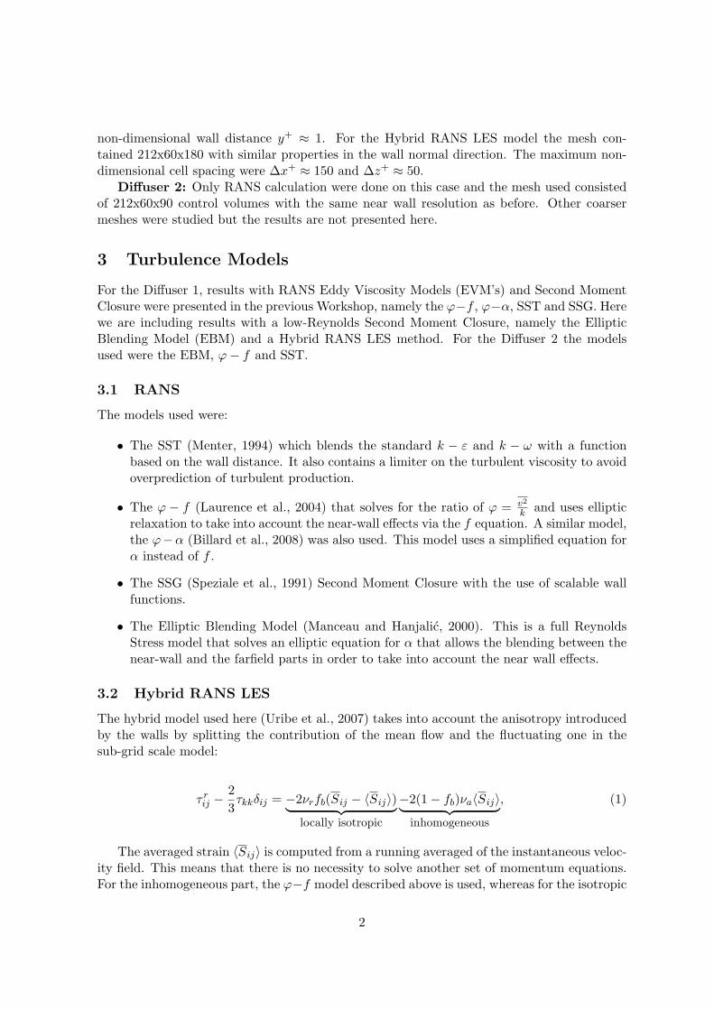
non-dimensional wall distance y+ ≈ 1. For the Hybrid RANS LES model the mesh con-tained 212x60x180 with similar properties in the wall normal direction. The maximum non-dimensional cell spacing were ∆x+ ≈ 150 and ∆z+ ≈ 50.
Diffuser 2: Only RANS calculation were done on this case and the mesh used consistedof 212x60x90 control volumes with the same near wall resolution as before. Other coarsermeshes were studied but the results are not presented here.
3 Turbulence Models
For the Diffuser 1, results with RANS Eddy Viscosity Models (EVM’s) and Second MomentClosure were presented in the previous Workshop, namely the ϕ−f , ϕ−α, SST and SSG. Herewe are including results with a low-Reynolds Second Moment Closure, namely the EllipticBlending Model (EBM) and a Hybrid RANS LES method. For the Diffuser 2 the modelsused were the EBM, ϕ− f and SST.
3.1 RANS
The models used were:
• The SST (Menter, 1994) which blends the standard k − ε and k − ω with a functionbased on the wall distance. It also contains a limiter on the turbulent viscosity to avoidoverprediction of turbulent production.
• The ϕ − f (Laurence et al., 2004) that solves for the ratio of ϕ = v2
k and uses ellipticrelaxation to take into account the near-wall effects via the f equation. A similar model,the ϕ−α (Billard et al., 2008) was also used. This model uses a simplified equation forα instead of f .
• The SSG (Speziale et al., 1991) Second Moment Closure with the use of scalable wallfunctions.
• The Elliptic Blending Model (Manceau and Hanjalic, 2000). This is a full ReynoldsStress model that solves an elliptic equation for α that allows the blending between thenear-wall and the farfield parts in order to take into account the near wall effects.
3.2 Hybrid RANS LES
The hybrid model used here (Uribe et al., 2007) takes into account the anisotropy introducedby the walls by splitting the contribution of the mean flow and the fluctuating one in thesub-grid scale model:
τ rij −
23τkkδij = −2νrfb(Sij − 〈Sij〉)︸ ︷︷ ︸
locally isotropic
−2(1− fb)νa〈Sij〉︸ ︷︷ ︸inhomogeneous
, (1)
The averaged strain 〈Sij〉 is computed from a running averaged of the instantaneous veloc-ity field. This means that there is no necessity to solve another set of momentum equations.For the inhomogeneous part, the ϕ−f model described above is used, whereas for the isotropic
2

part, the Smagorinsky (1963) model is used. The turbulent viscosity corresponding to eachpart are computed as follows:
νr = (Cs∆)2√
2(Sij − 〈Sij〉
) (Sij − 〈Sij〉
)(2)
νa = CµϕkT with T = max(
kε , CT
√νε
)(3)
Finally the blending function fb is used to avoid double counting of the stresses and tomake sure that the RANS contribution diminishes as the mesh is refined. It is calculated as:
fb = tanh(
1.5Lt
∆
)(4)
For the inlet conditions the Synthetic Eddy Method of Jarrin et al. (2006) was used inorder to obtain an artificial turbulent field.
4 Results
4.1 Diffuser 1
The Eddy viscosity models failed to capture the separation on the correct wall as seen onthe previous ERCOFTAC workshop. Here both the EBM and the Hybrid model predict theseparation on the top inclined wall as reported on the experiments (see figure 2).
Figure 2: Velocity profiles for diffuser 1.
4.1.1 Diffuser 2
The separated zone on the second diffuser is on the side wall rather than on the upper wallas with the previous geometry. Here all models predict the separation region on this side wallbut with different lengths (see figure 3).
The SST model predicts the separation starting point on the lower corner (straight)whereas the experiments show that separation starts on the upper corner (diverging). Theϕ − f model predicts the start of the separation on the correct corner but the size of the
3

Figure 3: Velocity profiles for diffuser 2.
re-circulation region is far too large. On the other hand, the EBM predicts a too smallre-circulation region but closer to the experiments. This can be seen in figure 4 where thestreamsiwe velocity contours are shown. The thick line represents the zero velocity line.
References
F. Archambeau, N. Mechitoua, and M. Sakiz. A finite volume method for the computationof turbulent incompressible flows - industrial applications. International Journal on FiniteVolumes, 1(1):1–62, 2004.
F. Billard, J. Uribe, and D. Laurence. A new formulation of the (v2 − f) model usingelliptic blending and its application to heat transfer prediction. In Engineering TurbulenceModelling and Experiments 7, pages 89–94, 2008.
E. M. Cherrye, C. J. Elkins, and J. K. Eaton. Geometric sensitivity of three-dimensionalseparated ows. International Journal of Heat and Fluid Flow, 29:803–811, 2008.
N. Jarrin, S. Benhamadouche, D. Laurence, and R. Prosser. A synthetic-eddy method forgenerating inflow conditions for large-eddy simulations. International Journal of Heat andFluid Flow, 27:585–593, 2006.
D. Laurence, J.C. Uribe, and S. Utyuzhnikov. A robust formulation of the v2-f model. Flow,Turbulence and Combustion, 73:169–185, 2004.
R. Manceau and K. Hanjalic. A new form of the elliptic relaxation equation to account forwall effects in RANS modelling. Physics of Fluids, pages 2345–2351, 2000.
F. R. Menter. Two-equation eddy-viscosity turbulence models for engineering applications.AIAA Journal, 32(8):1598–1605, 1994.
J. Smagorinsky. General circulation experiments with the primitive equations: I the basicequations. Monthly Weather Review, 91:99–164, 1963.
4

a)
b)
c)
d)
Figure 4: Streamwise velocity contours at locations X/H = 2, 5, 8 and 12. a) Experiments,b) SST, c) ϕ− f , d) EBM
C.G. Speziale, S.Sarkar, and T.B. Gatski. Modelling the pressure-strain correlation of turbu-lence: an invariant dynamical system approach. Journal of Fluid Mechanics, pages 245–272,1991.
J. Uribe, N. Jarrin, R. Prosser, and D. Laurence. Hybrid v2f rans les model and syntheticinlet turbulence applied to a trailing edge flow. In Turbulence and Shear Flow Phenomena,pages 701–706, 2007.
5

13th ERCOFTAC Workshop onRefined Turbulence ModellingSeptember 25-26, 2008, Graz, Austria
13th ERCOFTAC-SIG15 WorkshopCase 13.2: 3-D Diffuser Flow (Diffuser 1)
K. Abe1
1Department of Aeronautics and Astronautics, Kyushu University,
Motooka, Nishi-ku, Fukuoka 819-0395, Japan, [email protected]
1. Turbulence ModelsIn this study, recently-developed Hybrid LES/RANS (HLR) and Large-Eddy-Simulation (LES)models were applied to the present test case as described below. As for the HLR simulation(HLRS), the model by Abe[1] was adopted for the sub-grid scale (SGS) stress. This modelintroduces an anisotropy-resolving non-linear eddy-viscosity model (NLEVM)[2] to improvethe prediction accuracy in the near-wall RANS region. Detailed description of the model isgiven in Abe[1]. It is noted that some modification was included in the LES region, wherethe SGS model proposed by Inagaki et al.[3] was adopted. In this study, pure LES was alsoperformed for comparison, where the aforementioned SGS model of Inagaki et al.[3] was usedfor the whole flow region.
2. Test Case and Computational ConditionsFigure 1 illustrates the schematic view of the present test case. The corresponding experimentwas carried out by Cherry et al.[4] and detailed data were provided for comparison. The ex-perimental facility has a long constant rectangular cross-section channel of height (H) 1cm andwidth (B) 3.33cm, resulting in the fully-developed flow at the end of the channel. The Reynoldsnumber is 10,000 based on the channel height and the bulk-mean velocity (Ub). This flow has ahighly three-dimensional separation in the diffuser region, which shows considerable sensitivityto the characteristics of the diffuser’s geometry.
The present calculations were performed with the finite-volume procedure STREAM (Lienand Leschziner[5]; Apsley and Leschziner[6]). This method uses collocated storage on a grid.The second-order central difference scheme is used for the discretization of each term, exceptfor the convection terms of turbulence energy and dissipation rate in HLRS that are discretizedby a TVD implementation of the QUICK scheme (Lien and Leschziner[7]). The solution al-gorithm is based on the SIMPLE scheme. As for the time integration, the second-order Crank-Nicolson scheme is employed.
In this study, the wall-fitted computational grid consisted of 251 (x) × 51 (y) × 91 (z)nodes. In all the calculations, no-slip conditions were specified at walls, and the wall-nearestnodes were placed at y+ < 1. At the outlet boundary, general zero streamwise gradients wereprescribed. As for the inlet boundary condition, unsteady velocity distributions were given atevery time step, where the data were taken from the calculations of fully-developed rectangularduct flow performed in advance. In this study, the time step of 1.5 × 10⁻²H/Ub was specifiedfor both LES and HLRS and the statistics were evaluated from the obtained unsteady data forthe time period of 300 H/Ub or longer.

2 13th ERCOFTAC-SIG15 Workshop
Side view11.3 deg
H= 1 cm
L=15 cm
4 cm
x
y
Top viewB= 3.33 cm
2.56 deg
4 cm
x
z
Figure 1: Schematic view of 3-D diffuser (Diffuser 1).
U=0
(a) LES
U=0
(b) HLRS
Figure 2: Zero-streamwise velocity line (z/B = 1/2).
3. ResultsRepresentative results are shown below. Figure 2 shows zero-streamwise velocity line at thecenter plane (i.e., z/B = 1/2). As seen in the figure, a massive separation is clearly seen inthe region along the upper wall for both LES and HLRS cases. For both the cases, the flowreattaches in the downstream straight duct region, the fact which corresponds generally to theexperiment of Cherry et al.[4]. Although LES and HLRS give a qualitatively similar trend, therecan be seen considerable difference in the separation point. Concerning LES, the separationoccurs just downstream of the inlet rectangular duct connecting with the diffuser. On the otherhand, as for HLRS, the flow does not separate there but a little downstream. This trend of HLRScorresponds better to the experiment.
Pressure coefficients on the lower wall at the center plane, i.e., z/B = 1/2, are shown inFig. 3. Figures 3 (a) and (b) show the results predicted by pure LES and HLRS, respectively.The pressure coefficient on the lower wall at the center plane increases in the diffuser region.There can be seen some remarkable difference in the predictions between LES and HLRS, beingcaused by an early separation in LES just downstream of the diffuser inlet.
The profiles of the mean velocity and the streamwise turbulence intensity are shown in Fig. 4(LES) and Fig. 5 (HLRS). Two sections are selected, i.e., the center plane and a plane close tothe side wall (z/B = 7/8). It is found again that the present LES returned an earlier separationin the diffuser region. It is expected that this early separation is mainly due to coarser gridresolution in the near-wall region.
To investigate this issue in more detail, resolved and modeled streamwise Reynolds-stresscomponents in the HLRS results are compared in Fig. 6. As seen in the figure, it dependson the streamwise location which component plays the dominant role. In the downstream re-

K. Abe 3
0 10 20–0.2
0
0.2
0.4
0.6
0.8
1
Exp.Cal.
x/H
Cp
0 10 20–0.2
0
0.2
0.4
0.6
0.8
1
Exp.Cal.
x/H
Cp
(a) LES (b) HLRS
Figure 3: Predictions of pressure coefficient at center plane (z/B = 1/2) on lower wall.
0 5 10 15 20
0
1
2
3
4
x/H=–2
x/H=2
x/H=6
x/H=10
x/H=15.5 x/H=18.5Exp. Cal.
1.0U/Ub
x/H
y/H
0 5 10 15 20
0
1
2
3
4
x/H=–2
x/H=2
x/H=6
x/H=10
x/H=15.5 x/H=18.5Exp. Cal.
1.0U/Ub
x/H
y/H
Mean velocity Mean velocity
0 5 10 15 20
0
1
2
3
4
x/H=–2
x/H=2
x/H=6
x/H=10
x/H=15.5 x/H=18.5Exp. Cal.
0.25u’/Ub
x/H
y/H
0 5 10 15 20
0
1
2
3
4
x/H=–2
x/H=2
x/H=6
x/H=10
x/H=15.5 x/H=18.5Exp. Cal.
0.25u’/Ub
x/H
y/H
Streamwise turbulence intensity Streamwise turbulence intensity
(a) z/B = 1/2 (b) z/B = 7/8
Figure 4: Computational results of LES.
gion of the diffuser, most turbulence is given by the resolved component. Once separationoccurs, turbulence structures tend to become larger and their motions are more active. There-fore, dominant structures can be directly captured with the present grid resolution. On the otherhand, in the diffuser-inlet region, the RNAS model contributes greatly to the reproduction ofthe near-wall turbulence. Note that this effect is obtained mainly by the introduction of an ap-propriate NLEVM to give the stress anisotropy more correctly. From this fact, it is found thatthe deference of the model performance between pure LES and HLRS is actually caused by theprediction accuracy in the diffuser-inlet near-wall region.
Acknowledgements
The computation was mainly carried out using the computer facilities at Research Institute forInformation Technology, Kyushu University. The author wishes to express his appreciationto Professor M.A. Leschziner of Imperial College, London, UK for the support in using theSTREAM code.

4 13th ERCOFTAC-SIG15 Workshop
0 5 10 15 20
0
1
2
3
4
x/H=–2
x/H=2
x/H=6
x/H=10
x/H=15.5 x/H=18.5Exp. Cal.
1.0U/Ub
x/H
y/H
0 5 10 15 20
0
1
2
3
4
x/H=–2
x/H=2
x/H=6
x/H=10
x/H=15.5 x/H=18.5Exp. Cal.
1.0U/Ub
x/H
y/H
Mean velocity Mean velocity
0 5 10 15 20
0
1
2
3
4
x/H=–2
x/H=2
x/H=6
x/H=10
x/H=15.5 x/H=18.5Exp. Cal.
0.25u’/Ub
x/H
y/H
0 5 10 15 20
0
1
2
3
4
x/H=–2
x/H=2
x/H=6
x/H=10
x/H=15.5 x/H=18.5Exp. Cal.
0.25u’/Ub
x/H
y/H
Streamwise turbulence intensity Streamwise turbulence intensity
(a) z/B = 1/2 (b) z/B = 7/8
Figure 5: Computational results of HLRS.
0 5 10 15 20
0
1
2
3
4
0 5 10 15 20
0
1
2
3
4
x/H=–2
x/H=2
x/H=6
x/H=10
x/H=15.5 x/H=18.5Exp.
0.05u’u’/Ub
2
x/H
y/H
0 5 10 15 20
0
1
2
3
4
x/H=–2
x/H=2
x/H=6
x/H=10
x/H=15.5 x/H=18.5
0.05u’u’/Ub
2
Resolved Modeled
x/H
y/H
0 5 10 15 20
0
1
2
3
4
x/H=–2
x/H=2
x/H=6
x/H=10
x/H=15.5 x/H=18.5
0.05u’u’/Ub
2
Resolved Modeled
x/H
y/H
x/H=–2
x/H=2
x/H=6
x/H=10
x/H=15.5 x/H=18.5Exp.
0.05u’u’/Ub
2
Resolved Modeled
x/H
y/H
0 5 10 15 20
0
1
2
3
4
0 5 10 15 20
0
1
2
3
4
x/H=–2
x/H=2
x/H=6
x/H=10
x/H=15.5 x/H=18.5Exp.
0.05u’u’/Ub
2
x/H
y/H
0 5 10 15 20
0
1
2
3
4
x/H=–2
x/H=2
x/H=6
x/H=10
x/H=15.5 x/H=18.5
0.05u’u’/Ub
2
Resolved Modeled
x/H
y/H
0 5 10 15 20
0
1
2
3
4
x/H=–2
x/H=2
x/H=6
x/H=10
x/H=15.5 x/H=18.5
0.05u’u’/Ub
2
Resolved Modeled
x/H
y/H
x/H=–2
x/H=2
x/H=6
x/H=10
x/H=15.5 x/H=18.5Exp.
0.05u’u’/Ub
2
Resolved Modeled
x/H
y/H
(a) z/B = 1/2 (b) z/B = 7/8
Figure 6: Resolved and modeled streamwise Reynolds-stress components in HLRS.
References1. Abe, K., A hybrid LES/RANS approach using an anisotropy-resolving algebraic turbu-
lence model. Int. J. Heat Fluid Flow, 26, 204-222, 2005.2. Abe, K., Jang, Y.J., and Leschziner, M.A., An investigation of wall-anisotropy expressions
and length-scale equations for non-linear eddy-viscosity models. Int. J. Heat Fluid Flow,24, 181-198, 2003.
3. Inagaki, M., Kondoh, T., and Nagano, Y., A mixed-time-scale SGS model with fixedmodel-parameters for practical LES. J. Fluids Eng., 127, 1-13, 2005.
4. Cherry, E.M., Elkins, C.J., and Eaton, J.K., Geometric sensitivity of three-dimensionalseparated flows, Int. J. Heat Fluid Flow, 29, 803-811, 2008.
5. Lien, F.S., and Leschziner, M.A., A general non-orthogonal collocated finite volume algo-rithm for turbulent flow at all speeds incorporating second-moment turbulence-transportclosure, Part 1: Computational implementation. Comput. Methods Appl. Mech. Engrg,114, 123-148, 1994.
6. Apsley, D.D. and Leschziner, M.A., Advanced turbulence modelling of separated flow ina diffuser. Flow, Turbulence and Combustion, 63, 81-112, 1999.
7. Lien, F.S., and Leschziner, M.A., Upstream monotonic interpolation for scalar transportwith application to complex turbulent flows. Int. J. Num. Meths. In Fluids, 19, 527-548,1994.

14th ERCOFTAC Workshop onRefined Turbulence ModellingSeptember 18, 2009, Rome, Italy
14th ERCOFTAC-SIG15 WorkshopCase 13.2: 3-D Diffuser Flow (Diffuser 2)
K. Abe1
1Department of Aeronautics and Astronautics, Kyushu University,
Motooka, Nishi-ku, Fukuoka 819-0395, Japan, [email protected]
1. Turbulence ModelsIn this study, recently-developed Hybrid LES/RANS (HLR) and Large-Eddy-Simulation (LES)models were applied to the present test case as described below. As for the HLR simulation(HLRS), the model by Abe[1] was adopted for the sub-grid scale (SGS) stress. This modelintroduces an anisotropy-resolving non-linear eddy-viscosity model (NLEVM)[2] to improvethe prediction accuracy in the near-wall RANS region. Detailed description of the model isgiven in Abe[1]. It is noted that some modification was included in the LES region, wherethe SGS model proposed by Inagaki et al.[3] was adopted. In this study, pure LES was alsoperformed for comparison, where the aforementioned SGS model of Inagaki et al.[3] was usedfor the whole flow region.
2. Test Case and Computational ConditionsFigure 1 illustrates the schematic view of the present test case. The corresponding experimentwas carried out by Cherry et al.[4] and detailed data were provided for comparison. The ex-perimental facility has a long constant rectangular cross-section channel of height (H) 1cm andwidth (B) 3.33cm, resulting in the fully-developed flow at the end of the channel. The Reynoldsnumber is 10,000 based on the channel height and the bulk-mean velocity (Ub). This flow has ahighly three-dimensional separation in the diffuser region, which shows considerable sensitivityto the characteristics of the diffuser’s geometry.
The present calculations were performed with the finite-volume procedure STREAM (Lienand Leschziner[5]; Apsley and Leschziner[6]). This method uses collocated storage on a grid.The second-order central difference scheme is used for the discretization of each term, exceptfor the convection terms of turbulence energy and dissipation rate in HLRS that are discretizedby a TVD implementation of the QUICK scheme (Lien and Leschziner[7]). The solution al-gorithm is based on the SIMPLE scheme. As for the time integration, the second-order Crank-Nicolson scheme is employed.
In this study, the wall-fitted computational grid consisted of 251 (x) × 51 (y) × 91 (z)nodes. In all the calculations, no-slip conditions were specified at walls, and the wall-nearestnodes were placed at y+ < 1. At the outlet boundary, general zero streamwise gradients wereprescribed. As for the inlet boundary condition, unsteady velocity distributions were given atevery time step, where the data were taken from the calculations of fully-developed rectangularduct flow performed in advance. In this study, the time step of 1.5 × 10⁻²H/Ub was specifiedfor both LES and HLRS and the statistics were evaluated from the obtained unsteady data forthe time period of 300 H/Ub or longer.

2 14th ERCOFTAC-SIG15 Workshop
Top viewB= 3.33 cm
4.0 deg
4.51 cm
x
z
Side view
9.0 degH= 1 cm
L=15 cm
3.37 cm
x
y
Figure 1: Schematic view of 3-D diffuser (Diffuser 2).
(a) 0 0.5 1 1.5–0.2
0
0.2
0.4
0.6
0.8
1
x/L
Cp
(b) 0 0.5 1 1.5–0.2
0
0.2
0.4
0.6
0.8
1
x/L
Cp
Figure 2: Pressure coefficient on lower wall at center plane (z/B = 1/2): (a) LES; (b) HLRS.
3. ResultsRepresentative results are shown below. Pressure coefficients on the lower wall at the centerplane, i.e., z/B = 1/2, are shown in Fig. 2. Figures 2 (a) and (b) show the results predicted bypure LES and HLRS, respectively. The pressure coefficient on the lower wall at the center planeincreases in the diffuser region. There can be seen some remarkable difference in the predictionsbetween LES and HLRS, being caused by an early separation in LES just downstream of thediffuser inlet.
The profiles of the mean velocity and the streamwise turbulence intensity are shown in Fig. 3(LES) and Fig. 4 (HLRS). Two sections are selected, i.e., the center plane and a plane close tothe side wall (z/B = 7/8). It is found again that the present LES returned an earlier separationin the diffuser region. Note that this fact was also seen in the results for the previous test case,i.e., “Diffuser 1.” It is expected that this early separation is mainly due to coarser grid resolutionin the near-wall region.
To investigate this issue in more detail, resolved and modeled streamwise Reynolds-stresscomponents in the HLRS results are compared in Fig. 5. As seen in the figure, it dependson the streamwise location which component plays the dominant role. In the downstream re-gion of the diffuser, most turbulence is given by the resolved component. Once separationoccurs, turbulence structures tend to become larger and their motions are more active. There-fore, dominant structures can be directly captured with the present grid resolution. On the otherhand, in the diffuser-inlet region, the RNAS model contributes greatly to the reproduction ofthe near-wall turbulence. Note that this effect is obtained mainly by the introduction of an ap-propriate NLEVM to give the stress anisotropy more correctly. From this fact, it is found thatthe deference of the model performance between pure LES and HLRS is actually caused by theprediction accuracy in the diffuser-inlet near-wall region.

K. Abe 3
0 5 10 15 20
0
1
2
3
4
x/H=–2
x/H=2
x/H=6
x/H=10
x/H=15.5 x/H=18.5
1.0U/Ub
x/H
y/H
0 5 10 15 20
0
1
2
3
4
x/H=–2
x/H=2
x/H=6
x/H=10
x/H=15.5 x/H=18.5
1.0U/Ub
x/H
y/H
Mean velocity Mean velocity
0 5 10 15 20
0
1
2
3
4
x/H=–2
x/H=2
x/H=6
x/H=10
x/H=15.5 x/H=18.5
0.25u’/Ub
x/H
y/H
0 5 10 15 20
0
1
2
3
4
x/H=–2
x/H=2
x/H=6
x/H=10
x/H=15.5 x/H=18.5
0.25u’/Ub
x/H
y/H
Streamwise turbulence intensity Streamwise turbulence intensity
(a) z/B = 1/2 (b) z/B = 7/8
Figure 3: Computational results of LES.
0 5 10 15 20
0
1
2
3
4
x/H=–2
x/H=2
x/H=6
x/H=10
x/H=15.5 x/H=18.5
1.0U/Ub
x/H
y/H
0 5 10 15 20
0
1
2
3
4
x/H=–2
x/H=2
x/H=6
x/H=10
x/H=15.5 x/H=18.5
1.0U/Ub
x/H
y/H
Mean velocity Mean velocity
0 5 10 15 20
0
1
2
3
4
x/H=–2
x/H=2
x/H=6
x/H=10
x/H=15.5 x/H=18.5
0.25u’/Ub
x/H
y/H
0 5 10 15 20
0
1
2
3
4
x/H=–2
x/H=2
x/H=6
x/H=10
x/H=15.5 x/H=18.5
0.25u’/Ub
x/H
y/H
Streamwise turbulence intensity Streamwise turbulence intensity
(a) z/B = 1/2 (b) z/B = 7/8
Figure 4: Computational results of HLRS.

4 14th ERCOFTAC-SIG15 Workshop
0 5 10 15 20
0
1
2
3
4
0 5 10 15 20
0
1
2
3
4
x/H=–2
x/H=2
x/H=6
x/H=10
x/H=15.5 x/H=18.5
0.05u’u’/Ub
2
Resolved Modeled
x/H
y/H
0 5 10 15 20
0
1
2
3
4
x/H=–2
x/H=2
x/H=6
x/H=10
x/H=15.5 x/H=18.5
0.05u’u’/Ub
2
Resolved Modeled
x/H
y/H
x/H=–2
x/H=2
x/H=6
x/H=10
x/H=15.5 x/H=18.5
0.05u’u’/Ub
2
Resolved Modeled
x/H
y/H
0 5 10 15 20
0
1
2
3
4
0 5 10 15 20
0
1
2
3
4
x/H=–2
x/H=2
x/H=6
x/H=10
x/H=15.5 x/H=18.5
0.05u’u’/Ub
2
Resolved Modeled
x/H
y/H
0 5 10 15 20
0
1
2
3
4
x/H=–2
x/H=2
x/H=6
x/H=10
x/H=15.5 x/H=18.5
0.05u’u’/Ub
2
Resolved Modeled
x/H
y/H
x/H=–2
x/H=2
x/H=6
x/H=10
x/H=15.5 x/H=18.5
0.05u’u’/Ub
2
Resolved Modeled
x/H
y/H
(a) z/B = 1/2 (b) z/B = 7/8
Figure 5: Resolved and modeled streamwise Reynolds-stress components in HLRS.
AcknowledgementsThe computation was mainly carried out using the computer facilities at Research Institute forInformation Technology, Kyushu University. The author wishes to express his appreciationto Professor M.A. Leschziner of Imperial College, London, UK for the support in using theSTREAM code.
References1. Abe, K., A hybrid LES/RANS approach using an anisotropy-resolving algebraic turbu-
lence model. Int. J. Heat Fluid Flow, 26, 204-222, 2005.2. Abe, K., Jang, Y.J., and Leschziner, M.A., An investigation of wall-anisotropy expressions
and length-scale equations for non-linear eddy-viscosity models. Int. J. Heat Fluid Flow,24, 181-198, 2003.
3. Inagaki, M., Kondoh, T., and Nagano, Y., A mixed-time-scale SGS model with fixedmodel-parameters for practical LES. J. Fluids Eng., 127, 1-13, 2005.
4. Cherry, E.M., Elkins, C.J., and Eaton, J.K., Geometric sensitivity of three-dimensionalseparated flows, Int. J. Heat Fluid Flow, 29, 803-811, 2008.
5. Lien, F.S., and Leschziner, M.A., A general non-orthogonal collocated finite volume algo-rithm for turbulent flow at all speeds incorporating second-moment turbulence-transportclosure, Part 1: Computational implementation. Comput. Methods Appl. Mech. Engrg,114, 123-148, 1994.
6. Apsley, D.D. and Leschziner, M.A., Advanced turbulence modelling of separated flow ina diffuser. Flow, Turbulence and Combustion, 63, 81-112, 1999.
7. Lien, F.S., and Leschziner, M.A., Upstream monotonic interpolation for scalar transportwith application to complex turbulent flows. Int. J. Num. Meths. In Fluids, 19, 527-548,1994.

Flow in a 3–D Diffuser: Simulations Based on a Hybrid
LES–URANS Approach and Pure LES
Michael Breuer
Professur fur Stromungsmechanik (PfS), Helmut–Schmidt–Universitat Hamburg,Holstenhofweg 85, D–22043 Hamburg, Germany
1 Introduction
The turbulent flow through a 3D diffuser is a quite new test case which was recently proposed forthe 13th ERCOFTAC Workshop on Refined Turbulence Modeling in Graz [1]. It is based on theexperimental measurements by Cherry et al. [2] who investigated two different configurations bythe magnetic resonance velocimetry. In contrast to most of the diffuser flows studied before, whichwere nominally 2D, a geometrically 3D setup is chosen which additionally avoids any symmetries toeliminate the problem of swapping separated flow regions between the two diverging walls. A longdevelopment channel with a rectangular cross-section of height h = 1 cm and aspect ratio of 1:3.33upstream of the diffuser guarantees a fully developed duct flow and thus clearly defined boundaryconditions at the inlet. The diffuser with a length of 15 cm is attached directly to the exit ofthe development channel and possesses either a square outlet (diffuser #1) or a rectangular outlet(diffuser #2), leading to area expansion ratios of 4.8 and 4.56, respectively. All walls are straight,except one side and the top wall which expands at different angle for diffuser #1 (side angle: 2.56
/ top angle: 11.3) and diffuser #2 (side angle: 4.0 / top angle: 9.0). The corners between thestraight and inclined walls are smoothed. The Reynolds number based on the height of the inletchannel and the bulk velocity is approximately 10,000. Additionally, an outlet transition device ismounted behind the diffuser, see [2]. As expected, a 3D boundary layer separation is observed in thediffuser. The strong adverse pressure gradient leads to a rapid boundary layer growth and finallyto flow separation which evolves differently for diffuser #1 and #2. The associated unsteadinessplays an important role yielding a turbulent flow with highly non-equilibrium characteristics whichrenders a challenge for turbulence modeling.
2 Turbulence Modeling
In the present study numerical simulations of the flow through diffuser #1 and # 2 are carriedout applying a hybrid LES–URANS approach. Additionally, large–eddy simulations using differentsubgrid–scale models are performed for diffuser #1.
2.1 Hybrid LES–URANS Methodology
The hybrid method proposed in [3–5] relies on the idea to apply RANS or more specifically URANSin those regions, where statistical turbulence models in general perform properly. Moreover, LESis used in regions, where large unsteady vortical structures are present, which should be resolveddirectly. Thus URANS is used for the near–wall region, whereas LES is performed in the remainingcomputational domain. Overall this approach reduces the resolution requirements since the ap-plication of RANS/URANS for the prediction of attached boundary layers allows to decrease the

near–wall resolution with the exception of the wall–normal direction. This raises the hope that hy-brid LES–URANS techniques can be used with acceptable effort even for high–Re flows encounteredin technical applications.When setting up a hybrid approach, several questions have to be answered. The main ones are:1. Which models should be used in the URANS and LES regions? 2. How should the LES–URANSinterface be defined? 3. How should both regions be coupled?In order to take the anisotropy of the Reynolds stresses in the near–wall region reasonably intoaccount, the explicit algebraic Reynolds stress model (EARSM) proposed by Wallin and Johans-son [6] is used. It represents a compromise between the too expensive full RSMs and classical lineareddy–viscosity models (LEVM) based on the Boussinesq approximation relating the shear stresscomponent to the mean velocity gradient. The latter are not capable to account for the stressanisotropy.For the implementation into a CFD code, the EARSM can be formally expressed in terms of a non–linear eddy–viscosity model (NLEVM). Its extra computational effort is small, still requiring solelythe solution of one additional transport equation for the turbulent kinetic energy. The non–closedstress tensor in the Reynolds–averaged momentum equations is written as [6]:
u′
iu′
jmod= kmod
(
2
3δij − 2 Ceff
µ Sij + a(ex)ij
)
(1)
Here, a(ex)ij = f(S2,Ω2, SnΩm, f1, ...) represents an extra tensor which takes the anisotropy of the
stresses into account and is computed explicitly based on the mean strain Sij and rotation tensorsΩij normalized by the turbulent time scale. As shown in [6] the model obtains the correct near–wallbehavior. The value of Cµ within the relation for the eddy viscosity νt = Cµ ·vc · lc is not a constant
but dynamically calculated, thus denoted Ceffµ .
However, the EARSM itself is not complete since the length scale lc and the velocity scale vc arenot defined. These have to be supplied by an additional scale–determining part. In principle, thatcan be achieved by a two–equation model such as a classical k–ǫ or k–ω model, which in the contextof RANS is a natural choice since one transport equation is solved for the velocity scale and onefor the length scale. However, for the present hybrid methodology a more or less unique modelingstrategy in both regions has several advantages. Since in LES the length scale is naturally givenby the filter width ∆, a one–equation model with a transport equation for the velocity scale ispreferred. Thus the length scale in the URANS region has to be defined by an algebraic relation.The resulting strategy consists of a single transport equation for the modeled turbulent kineticenergy kmod = kRANS = v2
c in RANS mode and the subgrid–scale (SGS) turbulent kinetic energykmod = kSGS in LES. This transport equation includes on the right-hand side the terms P, D,and ǫ, where P = −(u′
iu′
j)mod ∂U i/∂xj represents the production term closed by relation (1).Thus, in the non–linear model for the RANS zone P is determined on the basis of the consistentReynolds stress formulation including the anisotropy term which compared to the originally appliedlinear model [3] improves the production term and subsequently kmod. Note that the extensionto EARSM is actually not used in the LES mode. The unknown diffusion term D can be closedby a classical gradient–diffusion approach as done for the LES zone and previously also for theRANS zone [3]. However, for EARSM the enhanced representation of the Reynolds stresses can beintroduced into D by applying the diffusion model of Daly and Harlow [7] which is preferred here.Finally, the dissipation rate ǫ needs to be defined. For the LES zone the dissipation rate is set to
ǫ = Cd k3/2SGS/∆ yielding the one–equation SGS model of Schumann [8]. For the URANS zone the
formulation of ǫ is overtaken from the near–wall one–equation model by Chen and Patel [9] relyingon an algebraic relation for the length scale.Based on previous experiences [3–5] the predefinition of LES and URANS regions is avoided inthe present approach and a gradual transition between both methods is assured. The dynamicinterface criterion [3] relies on the modeled turbulent kinetic energy and the wall distance leading
2

to y∗ = k1/2mod · y/ν ≤ Cswitch,y∗ . For y∗ ≤ Cswitch,y∗ the method works in URANS mode, otherwise
the LES mode is applied. In principle, the constant Cswitch,y∗ allows the user to vary the averageinterface position and to study its effect. For the diffuser case at the moderate Reynolds numberconsidered, Cswitch,y∗ = 60 is set. In general, it should be defined so that the interface is located inthe logarithmic wall layer. However, it is worth to mention that the instantaneous interface positionstrongly varies in space and time depending on the local flow field close to the wall. Thus it reliesupon physical quantities accounting for characteristic flow properties and automatically reacts ondynamic flow field variations. This interface criterion partially provides no sharply delimited LES–URANS regions. Therefore, an enhanced version guaranteeing a sharp interface without RANSislands was also taken into account, see, e.g., [3–5]. This investigation confirmed that the RANSislands found for the basic version do not influence the results. Thus in the present study thisoriginal interface criterion is applied.
2.2 Large–Eddy Simulation
In addition to the hybrid approach, the pure LES technique is applied to generate data for com-parison. For modeling the non–resolvable subgrid scales, two different models are applied, namelythe well–known Smagorinsky model [10] with Van Driest damping near solid walls (Cs = 0.065)and the dynamic approach with a Smagorinsky base model proposed by Germano et al. [11] andmodified by Lilly [12]. In order to stabilize the dynamic model, averaging of the numerator and thedenominator in the relation for the determination of the Smagorinsky value [11,12] was carried outin time using a recursive digital low–pass filter [13].
3 Numerical Method
The LES code LESOCC used for the solution of the filtered Navier–Stokes equations, is a 3–Dfinite–volume solver for arbitrary non–orthogonal and non–staggered grids [13, 14]. The spatialdiscretization of all fluxes is based on a central scheme of second–order accuracy. A low–storagemulti–stage Runge–Kutta method is applied for time–marching. The additional transport equationfor kmod is discretized with the same scheme. Beside the hybrid approach different SGS modelsfor LES are implemented as well as DES. These features are used to provide reference data forcomparison with the hybrid method.
4 Details of the Test Case
Since both diffusers are geometrically comparable, first all common features are provided and dif-ference between diffuser #1 and #2 are given separately.
4.1 Computational Domain
Block–structured grids were generated which cover a computational domain including an inlet duct(−5 ≤ x/h ≤ 0, height h, aspect ratio 1:3.33), the diffuser itself (0 ≤ x/h ≤ 15) and an outletduct (15 ≤ x/h ≤ 27.5) with either a 4 cm square cross-section for diffuser #1 or a rectangularcross-section (height 3.37 cm × 4.51 cm width). In order to avoid a recirculation at the outlet, acontracting duct (27.5 ≤ x/h ≤ 37.5) with a 3 cm square cross-section at the tail was attached toboth diffusers.
4.2 Boundary Conditions
A precursor simulation of a 1:3.33 duct flow with periodic boundary conditions in streamwise di-rection was used to provide reliable inflow data at the inlet duct located x/h = −5. These duct
3

flow simulations (one for the hybrid simulations and one for the LES predictions) were carried outapplying grids which possess the same cross–sectional grid distributions and the same time stepsizes. Thus any interpolation in space and time could be avoided and the data of one cross-sectionof the duct flows were directly applicable at the inlet of the diffusers. No–slip boundary conditionswere imposed at all walls and a convective outflow boundary condition was applied at the outlet.
4.3 Grids
Two different grids, a coarse one for the hybrid simulations and a fine one for the LES predictionswere generated. The coarse grid consists of about 3.25 million control volumes (CVs) with 62 ×
134 CVs in the cross-section and 392 CVs in streamwise direction. The grid points are clusteredtowards the walls. At the diffuser inlet a near–wall resolution of (∆y; ∆z)min,CV /h = 2.33 × 10⁻³
is used, whereas due to the larger cross-section the near–wall resolution at the diffuser outlet is(∆y; ∆z)min,CV /h = 5. × 10−3. For parallel computing the domain is decomposed into 6 equalblocks.The fine grid for the LES predictions of diffuser # 1 consists of more than five times more grid points,i.e., about 17.6 million control volumes (CVs) in total. Here the cross-section is discretized with128 × 256 CVs and 537 CVs are distributed in streamwise direction. The near–wall resolutions atthe diffuser inlet and outlet are (∆y; ∆z)min,CV /h = 2.0× 10⁻³ and (∆y; ∆z)min,CV /h = 4.× 10−3,respectively. For parallel computing the domain is decomposed into 24 equal blocks.
4.4 Cases Considered
For diffuser #1 a hybrid simulation on the coarse grid and three LES predictions on the fine gridapplying the Smagorinsky model, the dynamic model and no SGS model were carried out. Fordiffuser #2 solely a hybrid simulation on the coarse grid was performed.
Table 1 summarizes the different cases and the most important parameters.
Simu- Diffuser Grid Turbulence Dimensionless Averaging
lation # (CVs) Model Time Step Time
HYB 1 62 × 134 × 392 Hybrid LES–URANS 0.003 > 5300
LES-D 1 128 × 256 × 537 LES, dynam. Smag. 0.002 > 2600
LES-S 1 128 × 256 × 537 LES, Smagorinsky 0.002 > 2500
LES-N 1 128 × 256 × 537 LES, no SGS 0.002 > 3400
HYB-2 2 62 × 134 × 392 Hybrid LES–URANS 0.003 > 2620
Table 1: Overview on Simulation Parameters.
5 Some Results of the Hybrid Approach
5.1 Diffuser #1
Fig. 1 depicts the time–averaged streamwise velocity at five cross-sections downstream of the inletof the diffuser located at x/h = 0. The bold line indicates zero-streamwise-velocity and thus inclosesthe recirculation region. The upper figures show the experimental measurements by Cherry et al. [2]whereas the lower ones are the predictions based on the hybrid method using EARSM. As visiblefrom both rows, the recirculation starts at the upper-right corner, which is the corner between the
4

(a) Exp.: x/h = 2 (b) Exp.: x/h = 5 (c) Exp.: x/h = 8 (d) Exp.: x/h = 12 (e) Exp.: x/h = 15
(f) Sim.: x/h = 2 (g) Sim.: x/h = 5 (h) Sim.: x/h = 8 (i) Sim.: x/h = 12 (j) Sim.: x/h = 15
Figure 1: Diffuser #1: Contours of the streamwise velocity, comparison of experimental [2] and predicteddata using the hybrid technique.
two diverging walls. At x/h = 5 (see Figs. 1(b) and 1(g)) the separation bubbles remain in thecorner. At the next cross-section shown at x/h = 8 it is obvious that the recirculation regions hasstarted to spread across the top of the diffuser. Further downstream at x/h = 12 and 15 a massiveseparation region is visible covering the entire top wall of the diffuser. Overall an excellent agreementbetween the hybrid LES–URANS prediction and the measurements is found. This circumstance isnot self–evident for some simulations carried out for the ERCOFTAC Workshop in Graz [1]. Moreprecisely, all RANS predictions based on eddy–viscosity models are found to predict qualitativelywrong results showing a separation region at the side wall and not at the top wall as observed inthe experiment and the hybrid simulation. RANS predictions based on RSM partially do a betterjob but still do not reach a similar level of agreement as the hybrid simulation.
5.2 Diffuser #2
Similar to Fig. 1 the time–averaged streamwise velocity contours at five cross-sections of diffuser# 2 are depicted in Fig. 2. Again the bold line indicates zero-streamwise-velocity. The upper rowshows the experimental measurements [2] whereas the lower row displays the predictions based onthe hybrid LES–URANS method. As expected based on the experimental results, the shape of theseparation bubble in diffuser #2 differs fundamentally from the recirculation zone found in diffuser#1. In contrast to diffuser #1 where the reverse–flow region spreads across the top wall, in diffuser#2 it remains localized near the sharp corner and the side wall. This trend is correctly reproducedby the hybrid simulation. The experimental data show a splitting of the reverse–flow region intotwo disconnected separation regions at x/h = 12. Since the hybrid simulation delivers a singleseparation region along the side wall at the corresponding axial position, this feature of the flow isnot correctly reproduced by the hybrid simulation and requires further investigations.
A more detailed evaluation of the results including the LES predictions of diffuser # 1 will beprovided at the workshop.
References
[1] Brenn, G., Jakirlic, S., Steiner, H. (eds.) (2008). 13th SIG15 ERCOFTAC Workshop on Refined
Turbulence Modeling, Graz, Austria, Sept. 25–26, 2008.
5

(a) Exp.: x/h = 2 (b) Exp.: x/h = 5 (c) Exp.: x/h = 8 (d) Exp.: x/h = 12 (e) Exp.: x/h = 15
(f) Sim.: x/h = 2 (g) Sim.: x/h = 5 (h) Sim.: x/h = 8 (i) Sim.: x/h = 12 (j) Sim.: x/h = 15
Figure 2: Diffuser #2: Contours of the streamwise velocity, comparison of experimental [2] and predicteddata using the hybrid technique.
[2] Cherry, E.M., Elkins, C.J., Eaton, J.K. (2008). Geometric Sensitivity of Three-Dimensional
Separated Flows, Int. J. Heat Fluid Flow, 29, 803–811.
[3] Breuer, M., Jaffrezic, B., Arora, K. (2008) Hybrid LES–RANS Technique Based on a One–
Equation Near–Wall Model, J. Theoretical and Computational Fluid Dynamics, 22(3–4), pp.157–187.
[4] Jaffrezic, B., Breuer, M. (2008) Application of an Explicit Algebraic Reynolds Stress Model
within an Hybrid LES–RANS Method, J. of Flow, Turbulence and Combustion, vol. 81(3), pp.415–448.
[5] Breuer, M., Aybay, O., Jaffrezic, B. (2008) Application of an Anisotropy Resolving Algebraic
Reynolds Stress Model within a Hybrid LES–RANS Method, Seventh Int. ERCOFTAC Work-shop on DNS and LES: DLES-7, Trieste, Italy, Sept. 8–10, 2008.
[6] Wallin, S., Johansson, A.V. (2000) An Explicit Algebraic Reynolds Stress Model for Incom-
pressible and Compressible Turbulent Flows, J. Fluid Mech., 403, 89–132.
[7] Daly, B.J., Harlow, F.H. (1970) Transport Equations in Turbulence, Phys. Fluids, 13, 2634–2649.
[8] Schumann, U. (1975) Subgrid–Scale Model for Finite–Difference Simulations of Turbulent Flows
in Plane Channels and Annuli, J. Computat. Physics, 18, pp. 376–404.
[9] Chen, H.C., Patel, V.C. (1988). Near–Wall Turbulence Models for Complex Flows Including
Separation, AIAA Journal, 26(6), 641–648.
[10] Smagorinsky, J. (1963). General Circulation Experiments with the Primitive Equations, I, The
Basic Experiment, Mon. Weather Rev., 91, 99–165.
[11] Germano, M., Piomelli, U., Moin, P., Cabot, W.H. (1991). A Dynamic Subgrid–Scale Eddy–
Viscosity Model, Phys. Fluids A, 3(7), 1760–1765.
[12] Lilly, D. K. (1992). A Proposed Modification of the Germano Subgrid–Scale Closure Method,Phys. Fluids A, 4(3), 633–635.
[13] Breuer, M. (2002). Direkte Numerische Simulation und Large-Eddy Simulation turbulenter
Stromungen auf Hochleistungsrechnern, Habilitationsschrift, Universitat Erlangen-Nurnberg,Berichte aus der Stromungstechnik, ISBN 3-8265-9958-6, Shaker Verlag, Aachen.
[14] Breuer, M. (1998). Large–Eddy Simulation of the Sub-Critical Flow Past a Circular Cylinder:
Numer. & Mod. Aspects, Int. J. Num. Meth. Fluids, 28, 1281–1302.
6

14th
ERCOFTAC SIG 15 Workshop on Refined Turbulence Modelling
Sapienza University of Rome
September 18, 2009
LES, Hybrid LES/RANS and RANS-SMC of
Turbulent Flow Separation in a 3-D Diffuser
G. Kadavelil1, M. Kornhaas
2, E. Sirbubalo
1, S. Šarić
1,*, D.C. Sternel
2, S.
Jakirlić1 and M. Schäfer
2
Technische Universität Darmstadt, Department of Mechanical Engineering 1Chair of Fluid Mechanics and Aerodynamics, Petersenstr. 30, D-64287 Darmstadt,
Germany, gkadavelil/esirbubalo/saric/[email protected] 2Chair of Numerical Methods in Mechanical Engineering, Dolivostr. 15, D-64293 Darmstadt,
Germany, kornhaas/sternel/[email protected]
Abstract - An incompressible fully-developed duct flow expanding into a diffuser whose upper and one side
walls are appropriately deflected (two diffuser configurations differing with respect to the expansion angles
were considered, Fig. 1), for which the experimentally obtained reference database was provided by Cherry et
al. (2008, 2009), was studied computationally by using LES (Large Eddy Simulation), DES (Detached Eddy
Simulation) and RANS-SMC (Reynolds-Averaged Navier-Stokes in conjunction with a high-Reynolds number
Second-Moment Closure model) methods. In addition, a zonal Hybrid LES/RANS (HLR; RANS –
Reynolds-Averaged Navier Stokes) method, proposed recently by Jakirlic et al. (2006, 2009) and Kniesner
(2008), has been applied. The flow Reynolds number based on the height of the inlet channel is Reh=10000.
The primary objective of the present investigation was the comparative assessment of the afore-mentioned
computational models in this flow configuration characterized by a complex three-dimensional flow separation
being the consequence of an adverse pressure gradient evoked by the duct expansion. The focus of the
investigation was on the capability of the different modelling approaches to accurately capture the size and
shape of the three-dimensional flow separation pattern and associated mean flow and turbulence features.
1. Introduction
Configurations involving three-dimensional boundary layer separation are among the most
frequently encountered flow geometries in technical practice. Accordingly, the methods
simulating them computationally have to be appropriately validated along with a detailed and
reliable reference database. However, the largest majority of the experimental benchmarks
being often used for computational methods and turbulence models validation relates to
internal, two-dimensional flow configurations, as e.g. flow over backward-facing and
forward-facing steps, fences, ribs, 2-D hills and 2-D bumps mounted on the bottom wall of a
plane channel. It is assumed that the influence of the side walls being located at an appropriate
distance from each other (according to Bradshaw and Wong, 1972, the minimum aspect ratio
– representing the ratio of the channel height to channel width - should be 1:10 in order to
eliminate the influence of the side walls) is not felt in the channel mid plane considered
*Present address: AREVA NP GmbH, Computational Fluid Dynamics and Mechanical Analysis (NEAA-G),
Keiserleistrasse 29, D-63067 Offenbach, Germany; [email protected]

14th
ERCOFTAC SIG15 Workshop on Refined Turbulence Modelling 2
experimentally. Consequently, the spanwise direction can be regarded as a homogeneous one,
the fact enabling the application of the periodic boundary conditions within a computational
framework (even 2D computations when using the RANS approach). By doing so, the real
three-dimensional nature of the flow is completely missed: strong secondary motion already
across the inlet section of the channel (characterized by jets directed towards the channel walls
bisecting each corner with associated vortices at both sides of each jet) induced by the
Reynolds stress anisotropy (whose correct capturing is an important prerequisite for a
successful computation) - which is, as generally known, beyond the reach of the
eddy-viscosity RANS model group, complex 3-D separation pattern spreading over duct
corners (corner separation and corner reattachment), etc. These circumstances were the prime
motivation for the recent experimental study of the flow in a three-dimensional diffuser
conducted by Cherry et al. (2008, 2009). A detailed reference database comprising the
pressure distribution along the bottom non-deflected wall, three-component mean velocity
field and the streamwise Reynolds stress component field within the entire diffuser section
was provided. The diffuser dimensions and the coordinate system are shown in Fig. 1. The
inlet flow corresponds to fully-developed turbulence, and the bulk inlet velocity is 1 m/s in the
x direction resulting in the Reynolds number based on the inlet channel height (h=1 cm) of
10000. The origin of the coordinates coincides with the intersection of the two non-expanding
walls at the beginning of the diffuser’s expansion.
Figure 1: Geometry of the 3-D diffuser configurations considered, Cherry et al. (2008). Not in scale;
all measures are in cm; length of the developing duct is 62.9 cm.

Kadavelil et al. 3
Two three-dimensional diffuser configurations with the same fully-developed channel
inlet but slightly different expansion geometries (the upper-wall expansion angle is reduced
from αUW1=11.3o to αUW2=9
o; the side-wall expansion angle is increased from αSW1=2.56
o to
αSW2=4o) were experimentally investigated, Cherry et al. (2008). Both diffuser flows are
featured by a three-dimensional boundary layer separation, but the size and shape of the
separation bubble exhibit a high degree of geometric sensitivity to the dimensions of the
diffuser. The first diffuser configuration (Fig. 1 upper) has served as the test case of the 13th
ERCOFTAC Workshop on refined turbulence modelling, Steiner et al. (2009). In addition to
different RANS models, the LES and LES-related methods (different seamless and zonal
hybrid LES/RANS (HLR) models; DES – Detached Eddy Simulation) were comparatively
assessed.
The main objective of the present work is the validation of the recently developed hybrid
LES/RANS method representing a two-layer model formulation, coupling a RANS model in
the wall layer with an LES in the core flow, in this complex flow geometry. In addition to the
experimental database, the results obtained are analyzed along the LES, DES (Spalart et al.,
1997) and RANS (the basic differential Reynolds-stress model due to Gibson and Launder,
1978) results performed using the same computational grid.
2. Computational method
2.1. Computational models
The present HLR (Hybrid LES/RANS) method represents a zonal (with a variable interface),
two-layer hybrid approach combining LES method in the outer layer and RANS method in the
near-wall layer. Presently, the low-Reynolds number k-ε model due to Launder and Sharma
(1974) was applied in the near-wall region. The subgrid-scale model due to Smagorinsky is
used in the core flow. The model coupling is realised via the turbulent viscosity, representing
an approach which enables the solution obtained by using one system of equations. Depending
on the flow zone, the turbulent viscosity is either computed from the RANS formulation:
2 /
tC f kµ µν ε= (1) or from the Smagorinsky model 2 2
t SGS SC Sν ν= = ∆ (2)
where the Smagorinsky constant CS takes the value of 0.1, ∆ represents the filter width and
S the strain rate magnitude. The interface values for k and ε representing actually the
boundary conditions for the corresponding equations in the RANS sub-region are obtained by
estimating the subgrid-scale kinetic energy and dissipation:
2
2 20.3 0.3SGS SGS Sk S C Sν= = ∆ , 2 3
2 2
SGS SGS SS C Sε ν= = ∆
(3)
Such a procedure provides the continuity in k and ε profiles across the interface.
Consequently, a fairly smooth transition of the turbulent viscosity νt is ensured in accordance
to the equations (1), (2) and (3). The decision whether the viscosity is to be computed by
RANS or LES formulations depends on the position of the interface between the two domains.
The interface can either be positioned at a certain y+ or at a certain wall distance. In both cases
this value can be fixed or vary according to the control parameter

14th
ERCOFTAC SIG15 Workshop on Refined Turbulence Modelling 4
mod
mod
*res
kk
k k=
+
(4)
which represents the ratio (fraction) of modelled to the total turbulent kinetic energy in the
LES region, averaged over all grid cells at the interface belonging to the LES domain. As soon
as this value exceeds about 20 %† the interface is moved farther from the wall. In contrast,
the interface will be moved towards the wall in the case of values below 20. More details
about the HLR method are given in Jakirlic et al. (2006, 2009) and Kniesner (2008).
The basic feature of the LES and DES methods used presently are as follows:
• LES (Large Eddy Simulation): the sub-grid scales were modelled by the Smagorinsky
(1963) formulation utilizing the dynamic determination of the model coefficient proposed
by Germano et al. (1991)
• DES (Detached Eddy Simulation): a seamless hybrid LES/RANS approach employing the
one-equation turbulence model by Spalart and Allmaras (S-A, 1994), based on the
transport equation for turbulent viscosity νt, to model the influence of the smallest,
unresolved scales on the resolved ones (e.g. Spalart et al., 1997; Travin et al., 2002) in the
LES sub-region of the solution domain. The same model operating in the RANS mode
was used to model the near-wall layer. The smooth transition from the near-wall RANS
layer to the off-wall LES region was achieved by switching the wall distance d in the
destruction term in the νt -equation to the representative grid spacing ∆DES in accordance
with the formulation: min(d, CDES ∆DES) with ∆DES=max(∆x, ∆y, ∆z)
• RANS: the model employed represents a version of the basic differential Reynolds Stress
Model proposed by Gibson and Launder (GL RSM, 1978). The model was used in
conjunction with the standard, high Reynolds number wall functions. The only difference
compared to the original GL formulation is in the model of the diffusion transport.
Presently, the model based on the Simple Gradient Diffusion Hypothesis with the
diffusion coefficient modelled in terms of the turbulent viscosity was applied.
2.2. Numerical method
LES, DES and hybrid LES/RANS. The computational results presented were obtained by
using the in-house code FASTEST (Flow Analysis by Solving Transport Equations
Simulating Turbulence) which uses a finite volume method for block-structured, body-fitted,
non-orthogonal, hexahedral meshes, [4]. Block interfaces are treated in a conservative manner,
consistent with the treatment of inner cell-faces. Cell centred (collocated) variable
arrangement and Cartesian vector and tensor components are used. The equations are
linearised and solved sequentially using an iterative ILU method. The velocity-pressure
coupling is ensured by the pressure-correction method based on the SIMPLE algorithm which
is embedded in a geometric multi-grid scheme with standard restriction and prolongation,
Briggs et al. (2000). The code is parallelized applying the Message Passing Interface (MPI)
technique for communication between the processors. The convective transport of all
variables was discretized by a second-order, central differencing scheme for LES and DES. In
†A typical value of 20% was adopted in the present work, corresponding approximately to the reference value an
LES resolution should comply with (Pope, 2000).

Kadavelil et al. 5
the case of the HLR method some upwinding is used for k and ε equations by applying the so
called “flux blending” technique. Time discretization was accomplished applying the
(implicit) Crank-Nicolson scheme.
RANS. The RANS computations were performed using the code Open-FOAM (Weller et al.,
1998, see also [9]), an open source Computational Fluid Dynamics toolbox, utilizing a
cell-center-based finite volume method on an unstructured numerical grid and employing the
solution procedure based on the implicit pressure algorithm with splitting of operators (PISO)
for coupling between pressure and velocity fields.
2.3. Computational details
LES. The solution domain comprising a part of the development duct (5 h), the diffuser
section (15 h), the outlet straight duct (12.5 h) as well as the convergent part (≈ 9 h) is meshed
with 3.55 Mio. grid cells: NxxNyxNz=408x64x136, Fig. 2. Two simulations with and without
SGS model have been performed (only the results obtained by using the SGS model are
shown here). The wall boundary layers are resolved with y+ values of approximately O(1).
According to the experimental setup of Cherry et al. (2008) the fully developed turbulent
channel flow has been computed with respect to the inflow generation:. These inlet data are
generated by a simultaneously running periodic channel flow simulation of a channel
(NxxNyxNz=48x64x136) with the same cross section as the diffuser inlet, Fig. 2 (see also Fig.
5). To allow the flow through the diffuser to influence the flow field in the development
channel a part (5 channel heights) of this channel has been modelled in front of the diffuser.
The turbulent flow fields in a cross section in the periodic channel are copied to this inlet
location. Fig. 5 displays a slice through the computational domain and the periodic channel
where the contours show the unsteady streamwise velocity component. The time step size
chosen corresponds to the Courant number being smaller than one. This leads to a
non-dimensional time step of ∆t=0.011 (normalized by the inlet channel parameters
Ubulk=1m/s and h=1cm). Averaging was performed for approximately 80000 time steps. The
simulations were carried out on 16 IBM Power 5 CPUs and a load balancing efficiency of
100%. This leads to a computational time per time step of approximately 14s.
Figure 2: Solution domain and computational mesh used in the LES simulation
DES and HLR. The inflow data were generated by a precursor simulation of the fully
developed duct flow using the respective models on the grid containing of
NxxNyxNz=78x62x134 cells. The solution domain for both simulations DES and HLR

14th
ERCOFTAC SIG15 Workshop on Refined Turbulence Modelling 6
comprised a part of the development duct (5 h), the diffuser section (15 h) and the straight
outlet duct (12.5 h). At its outlet cross-section the convective outflow conditions were applied.
No-slip boundary conditions were applied at the walls. The grid applied in both simulations
contained NxxNyxNz=224x62x134 cells (approximately 1.86 Mio. grid cells in total; the
number of grid cells in the cross-plane y-z corresponds to that applied in the LES simulation).
The dimensionless time step ∆t=0.028 was used in the computations providing the CFL
number less than unity throughout the solution domain (CFLmax ≈ 0.76). The near-wall
resolution corresponds to ∆y+<0.8, ∆x
+≈10-100 and ∆z
+≈2-20 (along the x-y plane at z/B=1/2)
for the HLR simulation, Fig. 3. Similar resolution was documented also in the case of the
DES simulation. The final position of the interface separating the near-wall (RANS; green
area in Fig. 4-left) and off-wall (LES; blue area in Fig. 4-left) sub-regions determined in
accordance with the criterion explained earlier (Eq. 4) corresponded to y+ ≈ 50 in the HLR
simulation. Fig. 4-right displays the interface position along the bottom and lower diffuser
walls in the central x-y plane (z/B=1/2) expressed in terms of the non-dimensional
wall-distance y+ related to the DES simulation.
Figure 3: Near-wall resolution expressed in wall units along the upper and lower walls in the central
x-y plane (z/B=1/2) in the HLR simulations
Figure 4: Interface position in the HLR simulation corresponding to y
+ ≈ 50 (left) and in the DES
simulation (right)
RANS. Solution domain dimensions correspond exactly to those adopted for the DES and
HLR methods. It is meshed by a grid being uniform in all three coordinate directions
containing of the 1.872 Mio. grid cells in total (NxxNyxNz=520x60x60; Nx=80+240+200). The
y+-values of the wall-closest cells are between 2.5 and 15.3, the higher values corresponding
to the inlet duct and the lower ones to the diffuser section (the linear velocity law was applied
in the cells where the y+-values were below 11.6), Fig. 5. The steady solution could only be

Kadavelil et al. 7
obtained if using the 1st order Upwind Differencing Scheme (UDS). Stable functioning of a
higher order scheme was only possible if computing the 3-D diffuser flow in unsteady manner.
Presently the 2nd
order Linear UDS scheme was applied. The latter computations are in
progress.
Figure 5: The y+ values of the wall-adjacent cells for the second 3-D diffuser configuration. Similar
values are obtained for the Diffuser 1.
Acknowledgements. The work of G. Kadavelil and M. Kornhaas is financially supported by
the Deutsche Forschungsgemeinschaft (DFG) within the German Collaborative Research
Center (SFB 568) “Flow and Combustion in Future Gas Turbine Combustion Chambers”.
References 1. Bradshaw, P., Wong, F.Y.F. The Reattachment and Relaxation of a Turbulent Shear Layer. J.
Fluid Mech., 52(1): 113-135
2. Cherry, E.M., Elkins, C.J. and Eaton, J.K. Geometric sensitivity of three-dimensional separated
flows. Int. J. of Heat and Fluid Flow, 29: 803-811, 2008.
3. Cherry, E.M., Elkins, C.J. and Eaton, J.K. Pressure measurements in a three-dimensional
separated diffuser. Int. J. of Heat and Fluid Flow, 30: 1-2, 2009
4. FASTEST-Manual. Chair of Numerical Methods in Mechanical Engineering, Department of
Mechanical Engineering, Technische Universität Darmstadt, Germany, 2005
5. Gibson, M.M., Launder, B.E. Ground Effects on Pressure Fluctuations in the Atmospheric
Boundary Layer. J. Fluid Mech., 86: 491-511, 1978
6. Jakirlić, S., Kniesner, B., Šarić, S. and Hanjalic, K. Merging near-wall RANS models with LES
for separating and reattaching flows. ASME Joint U.S.-European Fluids Engineering Summer
Meeting: Symposium on DNS, LES and Hybrid RANS/LES Techniques, Miami, FL, USA, July,
17-20, Paper No. FEDSM2006-98039, 2006.
7. Jakirlić, S., Kniesner, B., Kadavelil, G., Gnirß, M. and Tropea, C. Experimental and
computational investigations of flow and mixing in a single-annular combustor configuration.
Flow, Turbulence and Combustion (Special issue: 7th Int. Symp. On Engineering Turbulence
Modelling and Measurements – ETMM7, Limassol, Cyprus, June 4-6, 2008), Vol. 83(3), 2009

14th
ERCOFTAC SIG15 Workshop on Refined Turbulence Modelling 8
8. Kniesner, B. Ein hybrides LES/RANS Verfahren für konjugierte Strömung, Wärme- und
Stoffübertragung mit Relevanz zu Drallbrennerkonfigurationen (A hybrid LES/RANS method for
conjugated flow, heat and mass transfer with relevance to swirl combustor configurations). PhD
Thesis, Technische Universität Darmstadt (http://tuprints.ulb.tu-darmstadt.de/950/), 2008.
9. OpenFOAM - The Open Source CFD Toolbox: www.opencfd.co.uk/openfoam/
10. Pope, S. Turbulent flows. Cambridge University Press, ISBN 0-521-59886-9, 2000
11. Spalart, P.R., Jou, W.-H., Strelets, M. and Allmaras, S. Comments on the feasibility of LES for
wings and on a hybrid RANS/LES approach, 1st AFOSR Int. Conf. on DNS and LES, Columbus,
OH, USA, August 4-8, 1997
12. Steiner, H., Jakirlić, S., Kadavelil, G., Šarić, S., Manceau, R. and Brenn. G. Report on 13th
ERCOFTAC Workshop on Refined Turbulence Modelling. September 25-26, 2008, Graz
University of Technology, ERCOFTAC Bulletin, No. 79, pp. 24-29, 2009
13. Travin, A., Shur, M., Strelets, M. and Spalart, P.R. Physical and numerical upgrades in the
Detached-Eddy Simulation of complex turbulent flows. In Fluid Mechanics and Its Application,
Friedrich and Rodi (eds.), Vol. 65, pp. 239-254, 2002
14. Weller, H.G., Tabor, G., Jasak, H. and Fureby, C., A tensorial approach to computational
continuum mechanics using object orientated techniques, Computers in Physics, Vol. 12, No. 6,
pp. 620-631, 1998

14th ERCOFTAC-SIG15 Workshop: 3D Diffuser – 2
H. Schneidera∗, D.A. von Terzia, H.–J. Bauera and W. Rodib
aInstitut fur Thermische Stromungsmaschinen, Universitat Karlsruhe (TH), 76128 Karlsruhe, GermanybInstitut fur Hydromechanik, Universitat Karlsruhe (TH), 76128 Karlsruhe, Germany
Abstract
Large–Eddy Simulation (LES) with the standard Smagorinsky model employing both wall-functionsand wall-resolving approaches was used to compute the flow in an asymmetric three-dimensional dif-fuser (test case 13.2). Different boundary conditions and parameters were tested in order to assessthe sensitivity of the computational results. It was shown that a LES using wall-functions is ableto compute all major flow-field characteristics in reasonable agreement with experimental data. Awall-resolving LES with an increased number of computational cells further improves the accuracyof the data, however, at a significantly higher cost.
1 Introduction
The 13th
ERCOFTAC-SIG15 workshop held in September 2008 at the Technical University of Graz [1]
showed that most Reynolds-Averaged Navier–Stokes (RANS) approaches have difficulties to predict the
three-dimensionally separated flow-field in an asymmetric diffuser. Large–Eddy Simulation (LES) on
the other hand was more promising since reasonable results could be achieved by the same authors
using equidistant grids together with wall-functions. This was confirmed in a LES study where both
diffusers were computed and good agreements with the experimental data was achieved [2]. In order
to better understand the potential and the limitations of LES with wall-functions in this flow, further
computations for the second diffuser have been conducted which are presented here.
2 Computational setup
Both the geometry and the Reynolds number for the simulations are in accordance with the diffuser-
experiments of Cherry et al. [3]. All values reported are made dimensionless using the bulk velocity
Ub = 1 m/s and the inlet channel height H = 1 cm, inlet channel width B = 3.33 cm or diffuser length
L = 15 cm as reference values. The Reynolds number based on the bulk velocity and the height of the
inlet channel was 10,000. The data presented was obtained using up to 280 processors on a HP Linux
cluster of the University of Karlsruhe. The different calculations conducted are briefly described in the
following.
2.1 Numerical method
All simulations were performed with the Finite Volume flow solver LESOCC2 (Large Eddy Simulation
On Curvilinear Coordinates) developed at the University of Karlsruhe [4]. This FORTRAN 95 program
solves the incompressible, three-dimensional, time-dependent, filtered or Reynolds-Averaged Navier–
Stokes equations on body-fitted, collocated, curvilinear, block-structured grids. Both the viscous and
convective fluxes are discretized with second-order accurate central differences. Time advancement is
accomplished by an explicit, low-storage Runge–Kutta method. Conservation of mass is achieved by
the SIMPLE algorithm with the pressure–correction equation being solved using the strongly implicit
procedure (SIP) of Stone. The momentum interpolation method of Rhie and Chow is employed to
prevent pressure–velocity decoupling and associated oscillations. Parallelization is achieved via a domain
decomposition technique with the use of ghost cells and MPI for the data transfer.
∗Email: [email protected], phone: +49 721 608-4703
1

Grid G1 G2 G3 G4
Domain length[−5; 23] [−5; 28] [−7; 28] [−7; 28]
x/H ∈
Nx 448 528 560 1190
Ny 60 60 60 164
Nz 60 60 60 220
Nx × Ny × Nz ≈ 1.6 × 10⁶
≈ 1.9 × 10⁶
≈ 2.0 × 10⁶
≈ 42.9 × 10⁶
Grid spacing equidistant stretched
Table 1: Details on computational grids.
Sim. Grid Wall BCAvg. time Buffer zone CPUhrs
PurposetUb/L x/H ∈ ×10
3
I G1 WF-H > 350 - < 16 LES-baseline
II G2 WF-H > 350 - < 18 outlet position sensitivity
III∗
G3 WF-H > 550 [26;28] < 20 inlet position sensitivity
IV G2 WF-WW > 550 [27;28] < 18 wall-function sensitivity
V G3 no-slip > 550 [26;28] < 20 wall-function sensitivity
VI∗
G4 no-slip > 150 [26;28] < 150 grid resolution
Table 2: Overview of simulations (* submitted results).
Sim.νt/νl
Reτ y+
wallz+
wall∆x+
max ∆y+max ∆z+
maxmean max.
III 0.15 0.47 560 4.7 15.5 35.0 9.3 31.1
VI 0.03 0.17 583 1.0 1.0 14.6 6.5 21.2
Table 3: Summary of mean flow properties of submitted results.
2.2 Computational domain and resolution
For the present study, simulations were performed using four different computational grids, having be-
tween 1.6 and 42.9 million grid cells. Table 1 compiles the major parameters of the various grids used.
All grids feature equidistant grid spacing in the streamwise direction. While one grid (G4) is stretched in
the two wall-normal directions in order to allow for wall-resolving simulations, the other grids (G1–G3)
are equidistant for use with wall-functions. Adaptive time-stepping ensured a CFL limit of less than 0.65
(with ∆t ≈ 0.01 − 0.004). In total between 500,000 and 600,000 time-steps were computed. Averaging
started after roughly 10 L/Ub, resulting in an averaging time of 125 – 650 L/Ub.
2.3 Turbulence model and boundary conditions
LES was performed on all grids using the standard Smagorinsky model [5] with Cs = 0.065 and van
Driest damping as a subgrid-scale model. For the grids with equidistant spacing in the wall-normal
directions two different wall-functions were tested: the one developed by Werner and Wengle [6], as well
as the one developed by Hinterberger [4].
Wall-function by Werner and Wengle (WF-WW) Here, u+is defined as the mean streamwise
velocity U normalized by the friction velocity uτ ≡
√
τw/ρ, where τw is the wall shear stress and ρthe density of the fluid, hence u+
≡ U/uτ . y+is defined as the distance from the wall y normalized by
the viscous length-scale δν ≡ ν√
ρ/τw = ν/uτ , where ν is the kinematic viscosity of the fluid, hence
y+≡ y/δν = uτy/ν. In this approach, the existence of a functional dependency of the form u+
= f(y+)
is assumed. This relation is used to determine the wall shear stress by applying it to the instantaneous
2
0 0.5 1U/U
b
0
0.25
0.5
0.75
1
1.25y/
HSim. ISim. IISim. IIIExp.
0 0.5 1U/U
b
0
0.5
1
1.5
0 0.5 1U/U
b
0
0.5
1
1.5
2
2.5
0 0.5 1U/U
b
0
0.5
1
1.5
2
2.5
3
0 0.5 1U/U
b
0
0.5
1
1.5
2
2.5
3
0 0.05 0.1V/U
b
0
0.25
0.5
0.75
1
1.25
y/H
0 0.05 0.1V/U
b
0
0.5
1
1.5
0 0.05 0.1V/U
b
0
0.5
1
1.5
2
2.5
0 0.05 0.1V/U
b
0
0.5
1
1.5
2
2.5
3
0 0.05 0.1V/U
b
0
0.5
1
1.5
2
2.5
3
Figure 1: Mean streamwise velocity U/Ub (top row) and mean vertical velocity V/Ub (bottom row) profiles atz/B = 0.5; from left to right: x/H = 2, 6, 10, 14 and 18.
data in the wall-adjacent cell using a 1/7–power law. Hence,
u+(y+
) =
y+; 0 ≤ y+ < y+
m
Cm(y+)m
; y+m
≤ y+,
where m = 1/7, Cm = 8.3 and y+m
= 11.81. For a given velocity and wall distance, τw is then obtained
directly.
Wall-function by Hinterberger (WF-H) The approach is similar to the one described above. How-
ever, instead of using a power law, Hinterberger used Direct Numerical Simulation (DNS) data of tur-
bulent channel flow at Reτ = 590 [7] that was approximated by eight piece-wise continuous functions
of the form
u+
i(y+
) =
y+if i = 1
Ai + Bi ln(y+) if i ∈ [2; 8]
,
where Ai and Bi are constants. For a given velocity and wall distance, τw is then obtained iteratively
using a Newton–Raphson method. The first segment resides in the region of y+ < 3 such that, for
wall-resolving simulations and at points with vanishing wall-shear, a no-slip condition is obtained. For
coarser grids, a wall-function assuming the existence of a logarithmic velocity profile is obtained.
At the outlet a convective BC is enforced in conjunction with a buffer zone in which the viscosity is
increased by a constant factor φ. Unsteady turbulent inflow data were generated by enforcing period-
icity in front of the domain within a section of length l/H = 3 and using a controller to enforce the
experimental mass flux. This is essentially a fully-developed channel flow simulation providing time-
dependant realistic flow structures for the diffuser.
2.4 Simulation overview
The different grids and wall boundary conditions used, as well as the averaging time and the CPU
hours for the various simulations are compiled in Tab. 2. Table 3 summarizes main flow properties
of the submitted results. The turbulent to laminar viscosity ratio νt/νl has been calculated using the
time-averaged turbulent viscosity. Mean refers to a time- and volume-average, while max. refers to
the maximum time-average of νt/νl. All wall units have been calculated in a mid-plane of the periodic
channel section.
3

0 0.5 1U/U
b
0
0.25
0.5
0.75
1
1.25y/
HSim. IIISim. IVSim. VExp.
0 0.5 1U/U
b
0
0.5
1
1.5
0 0.5 1U/U
b
0
0.5
1
1.5
2
2.5
0 0.5 1U/U
b
0
0.5
1
1.5
2
2.5
3
0 0.5 1U/U
b
0
0.5
1
1.5
2
2.5
3
0 0.5 1U/U
b
0
0.25
0.5
0.75
1
1.25
y/H
0 0.5 1U/U
b
0
0.5
1
1.5
0 0.5 1U/U
b
0
0.5
1
1.5
2
2.5
0 0.5 1U/U
b
0
0.5
1
1.5
2
2.5
3
0 0.5 1U/U
b
0
0.5
1
1.5
2
2.5
3
Figure 2: Mean streamwise velocity U/Ub profiles at z/B = 0.125 (top row) and z/B = 1 (bottom row); fromleft to right: x/H = 2, 6, 10, 14 and 18.
3 Results
3.1 Inlet and outlet position influence
In order to investigate the influence of the inlet and outlet position on the LES results for the coarse
equidistant grid, simulations I–III were conducted. Figure 1 shows streamwise U/Ub and vertical V/Ub
velocity profiles for simulations I–III and the experimental data at various streamwise locations along
the centerline. The velocity profiles indicate a negligible influence of the inlet and outlet position on the
velocity for these locations. The streamwise velocity is slightly overpredicted for z/B > 6 for locations
y/H < 1.5. However, all simulation results are in satisfactory agreement with the experimental data.
Another interesting result is that the use of a buffer zone greatly enhances computational performance
since it leads to a significant reduction of the time-step, see averaging time of simulations I–III in Tab. 2.
3.2 Wall-function influence
The influence of the wall boundary conditions on the results for the coarse equidistant grid may be
studied with Fig. 2. Streamwise U/Ub velocity profiles for simulations III–V are compared with the
experimental data at lateral locations z/B = 0.125 and 1, i.e. closer to the side-walls. Close to the
non-expanding side-wall at z/B = 0.125, see Fig. 2 top, the simulations almost coincide. At the z/B = 1
locations, however, the simulations deviate mostly among each other for x/H < 10 locations. The two
wall-functions yield almost the same results, which might be due to their conceptual similarity. At
the non-expanding side-wall, the quality of the results decreases for increasing streamwise location for
y/H > 1.5 locations. Conversely, the results quality increases for increasing streamwise locations at the
expanding side-wall (this is also due to the increasing wall-distance for increasing streamwise location).
The wall-function has difficulties in predicting the onset of separation at the corner of the two expanding
walls, but once separation is established the LES is able to compute the flow-field characteristics with
fair accuracy.
3.3 Resolution influence
We now compare the LES results obtained with the coarse equidistant grid (simulation III) and the finer
wall-resolving grid (simulation IV); these are the results which were submitted. Figures 3 and 4 show
U/Ub velocity contours at planes parallel to the two expanding and non-expanding walls, respectively,
of simulations III and VI, and the experiment. These are the most interesting locations since deviations
are most obvious here. Both LES are able to replicate the flow-field characteristics and the three-
4

x/H
z/B
0 2 4 6 8 10 12 14
0
0.5
1
z/B
0
0.5
1
z/B
0
0.5
1
y/H
0
1
2
3
y/H
0
1
2
3
x/H
y/H
0 2 4 6 8 10 12 140
1
2
3
Figure 3: Mean streamwise velocity U/Ub contours in a plane parallel to and ≈ 0.1B away from the top (left) andside (right) expanding wall; from top to bottom: experiments [3], simulations VI and III. Same velocity contourswith interval 0.1 shown for all plots; thicker line indicates zero-velocity contour.
z/B
0
0.5
1
z/B
0
0.5
1
x/H
z/B
0 2 4 6 8 10 12 14
0
0.5
1
y/H
0
1
2
3
y/H
0
1
2
3
x/H
y/H
0 2 4 6 8 10 12 140
1
2
3
Figure 4: Mean streamwise velocity U/Ub contours in a plane parallel to and 0.1B away from the bottom (left)and side (right) non-expanding wall; from top to bottom: experiments [3], simulations VI and III. Same velocitycontours with interval 0.1 shown for all plots; thicker line indicates zero-velocity contour.
dimensionality of the two recirculation bubbles close to the upper and lower wall of the diffuser (see
Fig. 3). Simulation III slightly overpredicts the size and extent of the recirculation bubbles in the
vicinity of the corner of the two expanding walls.
3.4 Transient effects
The dynamics of the large-scale turbulent motions in the diffuser exhibit a high level of unsteadiness.
Analysis of transient data shows that the separation bubble changes its size and extent as a function of
time. Figure 5 depicts the fraction of instantaneous negative to net mass flux Γ in a plane at x/H = 12
over 120 diffuser flow through times tUb/L (simulation II). It is difficult to identify regular shedding
patterns and analysis of instantaneous velocity signals did not yield distinct frequencies. It was found
due to the lack of homogeneous directions and low frequency unsteadiness in the flow that long averaging
5

0 20 40 60 80 100 120tU
b/L
0
2
4
6
8
10
Γ
Figure 5: Instantaneous fraction of negative to net mass flux Γ in a plane at x/H = 12 of simulation II. Horizontallines indicate mean values (solid line) and sum of mean values and standard deviation (dotted line) of Γ; samplesize n = 5000.
of the order O(102L/Ub) was required for sufficiently accurate mean values.
4 Conclusions
LES using the standard Smagorinsky model with both near-wall modelling and wall-resolving techniques
were conducted to compute the three-dimensionally separated flow in an asymmetric diffuser. Different
boundary and flow conditions were parametrically applied to a coarse equidistant grid employing wall-
functions. It was shown that for a given number of computational cells the flow is rather insensitive to the
wall-function used. Furthermore, a placement of the inlet boundary of two inlet channel heights upstream
of diffuser entry was found sufficient. The application of a buffer zone in conjunction with a convective
outlet boundary condition enhances time-stepping and therefore computational performance. Albeit
the LES with near-wall modelling used significantly fewer computational cells than the wall-resolving
simulation, it was able to predict all major flow-field characteristics within measurement uncertainty.
The wall-resolving LES delivered more accurate results, however, at significantly higher costs.
Acknowledgments
The work reported here was carried out within the “Research Group Turbo-DNS” at the Institut fur
Thermische Stromungsmaschinen. Its financial support by means of the German Excellence Initiative and
Rolls–Royce Deutschland is gratefully acknowledged. The authors appreciate the provision of computer
time by the Steinbuch Centre for Computing.
References
[1] G. Brenn, S. Jakirlic, and H. Steiner, editors. Proceedings of the 13th SIG15 ERCOFTAC/IAHR Workshopon Refined Turbulence Modelling, 25–26 September 2008, Graz University of Technology, Graz, Austria, GrazUniversity of Technology, Austria, September 2008.
[2] H. Schneider, D.A. von Terzi, H.-J. Bauer, and W. Rodi. Reliable and accurate prediction of three-dimensionalseparation in asymmetric diffusers using Large–Eddy Simulation. ASME paper GT2009–60110, 2009.
[3] E.M. Cherry, C. Elkins, and J.K. Eaton. Geometric sensitivity of three-dimensional separated flows. Int. J.Heat and Fluid Flow, 29(3):803–811, 2008.
[4] C. Hinterberger. Dreidimensionale und tiefengemittelte Large-Eddy-Simulation von Flachwasserstromungen.PhD Thesis, Universitat Karlsruhe (TH), Karlsruhe, Germany, 2004.
[5] J. Smagorinsky. General circulation experiments with the primitive equations. I: The basic experiment.Month. Weath. Rev., 91:99–165, 1963.
[6] H. Werner and H. Wengle. Large-eddy simulation of turbulent flow over and around a cube in a plate channel.In Schumann et al., editor, 8th Symposium on Turbulent Shear Flows. Springer Verlag, Berlin, 1993.
[7] R. Moser, J. Kim, and N. Mansour. Direct numerical simulation of turbulent channel flow up to Reτ = 590.Phys. Fluids, 1999.
6
1
DNS of 3D Diffuser 1 (test case 13.2),14th ERCOFTAC-SIG15 Workshop
By Johan Ohlsson∗, Philipp Schlatter∗, Paul F. Fischer† & Dan S.Henningson∗
∗Linne Flow Centre, Department of MechanicsRoyal Institute of Technology, SE-100 44 Stockholm, Sweden
† MCS, Argonne National Laboratory, 9700 S. Cass Avenue, Argonne, IL 60439, USA
(Received 1 September 2009)
A direct numerical simulation (DNS) of turbulent flow in a three-dimensional diffuser atRe = 10 000 was performed with a massively parallel high-order spectral element code onup to 32 768 cores. Mean flow results are in excellent agreement with experimental data.It is thus shown that DNS of complex flows, featuring e.g. pressure-induced separationin three dimensions, is possible at realistic Reynolds numbers with high accuracy evenin complicated geometries.
1. Numerical method and simulation setup
The spectral-element method (SEM), introduced by Patera (1984), is a high-orderweighted residual technique similar to the finite element method (FEM), where the mostpronounced difference is the particular Gauss-Lobatto-Legendre (GLL) grid employed inSEM. This enables exact integration even for high order polynomials, whereas the localelement retains the geometrical flexibility. SEM has opened the possibility to study – ingreat detail – fluid phenomena known to be very sensitive to discretization errors, e.g.flows undergoing pressure-induced separation (Ohlsson et al. 2008).
Here, the incompressible Navier–Stokes equations in R3,
∂u
∂t+ u · ∇u = −∇p +
1
Re∇
2u in Ω, ∇ · u = 0 in Ω (1.1)
are considered, where u is the velocity, p is the pressure and Re = UL/ν the Reynoldsnumber based on characteristic velocity and length scales, U and L respectively. Asfor FEM, the starting point for a SEM discretization is to cast the problem in theweak formulation, in which Eq. 1.1 is multiplied by a test function (v, q) ∈ H1
0 (Ω) andintegrated over Ω. The viscous term is integrated by parts so that the highest existentderivative is of first order. The problem (1.1) then becomes: Find (u, p) ∈ H 1
0such that
d
dt(v,u) + (v,u · ∇u) = (p,∇ · v) −
1
Re(∇v,∇u), (∇ · u, q) = 0, ∀(v, q) ∈ H1
0 (1.2)
where the inner products, (·, ·) are defined as
(v, u) :=
∫
Ω
vu dx. (1.3)
The discretization proceeds by the Galerkin approximation, where the test and trialspaces are restricted to the velocity and pressure spaces XN and Y N
⊂ H10 respectively
following the PN −PN−2 SEM discretization by Maday et al. (1987). The FEM and SEM

2 J. Ohlsson, P. Schlatter, P. F. Fischer and D. S. Henningson
differ by the choice of XN . For SEM this is typically a space of Nth-order Lagrange poly-nomial interpolants, hN
i (x), based on tensor-product arrays of GLL quadrature points ina local element, Ωe, e = 1, ..., E, satisfying hN
i (ξNj ) = δij , ξN
j ∈ [−1, 1] being one of the
N + 1 GLL quadrature points and δij is the Kronecker delta. For a single element in R3
the representation of u ∈ XN is
u(xe(r, s, t))|Ωe =N
∑
i=0
N∑
j=0
N∑
k=0
ueijkhN
i (r)hNj (s)hN
k (t) (1.4)
where xe is the coordinate mapping from the reference element Ω to the local element Ωe
and uijk is the nodal basis coefficient. Inserting the SEM approximation Eq. (1.4) intoEq. (1.2) and employing Gaussian quadrature for the integrals, yields the semi-discretizedequation
Bdu
dt= DT p − C(u)u −
1
ReKu, Du = 0 (1.5)
where B and K are the spectral-element mass and stiffness matrices respectively, C(u)denotes the non-linear operator and D is the discrete divergence operator. Temporaldiscretization of Eq. (1.5) is based on high-order splitting techniques, described in Madayet al. (1990). The non-linear terms are treated explicitly by third-order extrapolation(EXT3), whereas the viscous terms are treated implicitly by a third-order backwarddifferentiation scheme (BDF3) leading to a linear symmetric Stokes system for the basiscoefficient vectors un and pn to be solved at every time step:
Hun− DT pn = Bfn, Dun = 0. (1.6)
H = 1
ReK+ 3
2∆tB is the discrete equivalent of the Helmholtz operator (− 1
Re∇
2+ 3
2∆t). In
the RHS, fn accounts for the non-linear terms and for the cases we have external forcingin the Navier–Stokes equations.
For our purposes, we use the SEM code nek5000 by Fischer et al. (2008). The compu-tational domain shown in Fig. 1a, is set up in close agreement to the diffuser geometryin the experiment. It consists of the inflow development duct, the diffuser expansion andthe converging section. The resolution of approximately 172 million grid points is ob-tained by a total of 127 750 local tensor product domains (elements) with a polynomialorder of 11 respectively. The simulation was performed on the Blue Gene/P at ALCF,Argonne National Laboratory (32 768 cores and a total of 4 million node hours) and onthe AMD Opteron cluster “Ekman” at PDC, Stockholm (2048 cores and a total of 2million node hours). The lack of homogeneous directions together with the fact that theflow showed pronounced instationarity with fluctuations on a wide range of scales calledfor long integration time in order to get converged statistics. Two flow-through (200 t∗,where t∗ = 1/ubulk) were performed in order to let the flow settle to an equilibrium statebefore turbulent statistics were collected over approximately 250 t∗. A snapshot clearlyhighlighting the complex unsteady features of the flow is given in Fig. 1b. In the inflowduct, turbulence is triggered by means of an unsteady trip forcing, which eliminates ar-tificial temporal frequencies which may arise from inflow recycling methods. The outflowcondition specifies a homogeneous Dirichlet condition for the pressure and a homoge-neous Neumann condition for the velocities. In addition, a “sponge region” is added atthe end of the contraction in order to smoothly damp out turbulent fluctuations, therebyeliminating spurious pressure waves to arise when energetic turbulent structures hit the

DNS of 3D Diffuser 1 (test case 13.2), 14th ERCOFTAC-SIG15 Workshop 3
(a)
x
yz 6Pq
(b)
Figure 1. (a) Grid of one of the diffuser geometries (“Diffuser 1”) showing the developmentregion, diffuser expansion, converging section and outlet. (b) Snapshot showing isocontours of0.4 · ub.
y+/z+
u+
100
101
102
1030
5
10
15
20
25
x
Re τ
0 10 20 30 40 50 60 700
200
400
600
800
1000
1200
z
y
0 0.2 0.4 0.6 0.80.7
0.8
0.9
1
z
y
0 0.2 0.4 0.6 0.80.7
0.8
0.9
1
(a) (b)
(c) (d)
Figure 2. (a) Mean centerplane velocity profile 13 x/h upstream of the diffuser throat whereu+(y+), u+(z+), turbulent channel flow simulation at Reτ = 590 Moser et al.
(1999), (b) evolution of Reτ in a middle plane of the inflow section, solid horizontal lines showingReτ for a periodic duct and vertical dashed line location of the selected velocity profile in (a),(c) Time-averaged flow field in one of the corners 13 x/h upstream of the diffuser throat showingthe secondary flow compared to (d) periodic duct simulation. Circles show approximate locationof vortex centers.
outflow boundary, as well as ensure the stability of the computation by preventing thesestructures from recirculating back into the domain.
2. Results
2.1. Inflow section
The turbulent inflow duct was studied in detail to ensure that a fully developed turbulentflow is reached at the end of the development section. Mean velocity profiles as a functionof y+ and z+ respectively taken from a middle plane a short distance upstream of thediffuser opening are shown in Fig. 2a.

4 J. Ohlsson, P. Schlatter, P. F. Fischer and D. S. Henningson
Good agreement with turbulent channel flow simulation at Reτ = 590 Moser et al.(1999) can be inferred. In particular, the linear profile in the viscous sublayer and thelog law is captured with good accuracy. Monitoring the streamwise development of thefriction Reynolds number, Reτ , see Fig. 2b, helps to detect where a fully turbulent flowis reached. The secondary flow in the corners of the duct also give a good indication onthe development of the flow and is known to be important for the correct separationbehavior (Cherry et al. 2008). As can be seen in Fig. 2c the corner vortices are capturedwell, compared to results from a periodic duct simulation in Fig. 2d. From the measureslisted above, we conclude that the flow has converged to a statistically stationary statewell upsteam of the diffuser throat.
2.2. Diffuser
Turning to the actual diffuser, a qualitative analysis focusing on identifying the size andlocation of the separated region is made by selecting a number of crossflow planes, shownin Fig. 3. At every crossflow location within the duct until the diffuser throat at x/h= 0, where h is the inlet channel height and x is the distance from the diffuser throat,there are no signs of separation, as expected. As soon as the diffuser starts to expand,the separation — as pointed out by Cherry et al. (2008) — increases rapidly due to theasymmetry in the geometry in the uppermost right corner, where the two inclined wallsmeet. As can be seen in Fig. 3a, at x/h = 2, the agreement between the experimental andsimulation data is excellent, both considering the flow in general the separated region inparticular. The separated flow in the uppermost right corner persists in both data setsuntil x/h = 5, shown by Fig. 3b, when it gradually spreads to the top of the diffuser.This spreading is present in both datasets, however, in slightly different ways. StudyingFig. 3c it is obvious that the separation in the experimental data advances like a wedgeover to the top and uppermost left corner of the diffuser. The simulation data on theother hand, indicate that the smaller separation from the left corner — visible in Fig. 3b— grows into a small, stretched localized region in the top of the diffuser, from where itrapidly continues to grow down into the interior of the diffuser, finally taking the shapeof a small “bump” hanging from the top wall at x/h = 8 (Fig. 3c). Shortly thereafter thisregion has grown together with the separated flow from the right. It should be pointedout that the flow was averaged for a long time and the “bump” in Fig. 3c showed nosigns of instationarity, and so it is not clear from where these differences stem. In therest of the diffuser region, the fraction of separated flow in a cross-section is more or lessidentical in both datasets, including the maximum of 23 % area separated flow occuringat x/h = 15 (Fig. 3d), where the straight part starts. The simulation data predicts thebulk of the separated flow to be located to the left, also indicated by the experimentaldata in Fig. 3d. This trend is present well inside the straight section until x/h = 20, afterwhich the separation is reduced to zero — a result supported by both data sets.
The streamwise rms-values, urms/ubulk · 100, given in Fig. 4 at the same crossflowlocations as the mean flow in Fig. 3 show a consistent picture of the flow dynamicspresent in the diffuser. Shortly after the diffuser throat the most dominant fluctuationsare found in the shear layer bounding the separation bubble in the uppermost right corner(Fig. 4a), reaching a magnitude of 22% of the bulk inlet velocity — also confirmed by theexperimental data. Further downstream, at x/h = 5 (Fig. 4b), the peak moves downwardand increases in magnitude (up to 25% of the bulk inlet velocity), indicating an intenseturbulence activity in this area. At x/h = 8 (Fig. 4c) the turbulent shear layer followsconsistently the spreading of the separation to the top wall of the diffuser, clearly seen inboth data sets. Due to the more pronounced region of separated flow to the left of the topwall in the simulation data the highest rms-values are found around (z, y) = (1.2, 1.6).

DNS of 3D Diffuser 1 (test case 13.2), 14th ERCOFTAC-SIG15 Workshop 5
0 1 2 30
0.5
1
z
y(a)
0 1 2 30
0.5
1
z
y
0
0.5
1
0 1 2 30
0.5
1
1.5
z
y
(b)
0 1 2 30
0.5
1
1.5
2
z y
0
0.2
0.4
0.6
0.8
0 1 2 30
0.5
1
1.5
2
2.5
z
y
(c)
0 1 2 30
0.5
1
1.5
2
2.5
z
y
0
0.2
0.4
0.6
0.8
0 1 2 30
0.5
1
1.5
2
2.5
3
3.5
z
y
(d)
0 1 2 3
0.5
1
1.5
2
2.5
3
3.5
4
z
y
−0.1
0
0.1
0.2
0.3
0.4
0.5
0.6
Figure 3. Crossflow planes of streamwise velocity 2, 5, 8 and 15 x/h downstream of the diffuserthroat. Left column: Computation by nek5000. Right column: Experiment by Cherry et al. (2008)Each streamwise position has its own colorbar on the right. Contour lines are spaced 0.1 · ubulk
apart. Thick black lines correspond to the zero velocity contour.
At x/h = 15, shown in Fig. 4d, the turbulence is more homogeneously spread over thecross-sectional area with a peak situated in the interior of the diffuer (around 17% of thebulk inlet velocity) — as can be seen in both data sets. A more quantitative comparisonis made in Fig. 5, where mean velocity profiles are selected in a spanwise midplane.Generally, excellent agreement is observed. In particular, the upward movement of thevelocity peak in the diffuser is well captured. The location and streamwise extensionof the separated region (here defined as a region with negative velocity) are in good
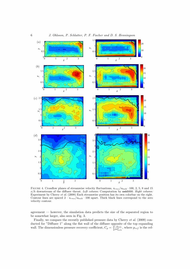
6 J. Ohlsson, P. Schlatter, P. F. Fischer and D. S. Henningson
0 1 2 30
0.5
1
z
y(a)
0 1 2 3
0.5
1
1.5
z
y
0
10
20
0 1 2 30
0.5
1
1.5
z
y
(b)
0 1 2 3
0.5
1
1.5
2
z y
0
5
10
15
20
0 1 2 30
0.5
1
1.5
2
2.5
z
y
(c)
0 1 2 3
0.5
1
1.5
2
2.5
z
y
0
5
10
15
20
0 1 2 30
0.5
1
1.5
2
2.5
3
3.5
z
y
(d)
0 1 2 3
0.5
1
1.5
2
2.5
3
3.5
4
z
y
0
5
10
15
20
25
30
Figure 4. Crossflow planes of streamwise velocity fluctuations, urms/ubulk · 100, 2, 5, 8 and 15x/h downstream of the diffuser throat. Left column: Computation by nek5000. Right column:Experiment by Cherry et al. (2008) Each streamwise position has its own colorbar on the right.Contour lines are spaced 2 · urms/ubulk · 100 apart. Thick black lines correspond to the zerovelocity contour.
agreement — however, the simulation data predicts the size of the separated region tobe somewhat larger, also seen in Fig. 3.
Finally, we compare the recently published pressure data by Cherry et al. (2009) con-ducted for ”Diffuser 1” along the flat wall of the diffuser opposite of the top expandingwall. The dimensionless pressure recovery coefficient, Cp =
p−pref1
2ρu2
bulk
, where pref is the ref-
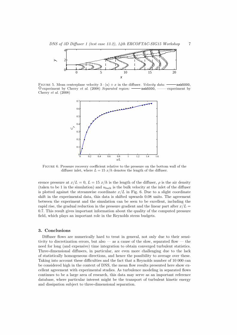
DNS of 3D Diffuser 1 (test case 13.2), 14th ERCOFTAC-SIG15 Workshop 7
x
y
0 5 10 15 200
2
4
Figure 5. Mean centerplane velocity 3 · 〈u〉 + x in the diffuser. Velocity data: nek5000, experiment by Cherry et al. (2008) Separated region: nek5000, experiment byCherry et al. (2008)
x/L
Cp
0 0.2 0.4 0.6 0.8 1 1.2 1.4 1.60
0.1
0.2
0.3
0.4
0.5
0.6
0.7
Figure 6. Pressure recovery coefficient relative to the pressure on the bottom wall of thediffuser inlet, where L = 15 x/h denotes the length of the diffuser.
erence pressure at x/L = 0, L = 15 x/h is the length of the diffuser, ρ is the air density(taken to be 1 in the simulation) and ubulk is the bulk velocity at the inlet of the diffuseris plotted against the streamwise coordinate x/L in Fig. 6. Due to a slight coordinateshift in the experimental data, this data is shifted upwards 0.08 units. The agreementbetween the experiment and the simulation can be seen to be excellent, including therapid rise, the gradual reduction in the pressure gradient and the linear part after x/L =0.7. This result gives important information about the quality of the computed pressurefield, which plays an important role in the Reynolds stress budgets.
3. Conclusions
Diffuser flows are numerically hard to treat in general, not only due to their sensi-tivity to discretization errors, but also — as a cause of the slow, separated flow — theneed for long (and expensive) time integration to obtain converged turbulent statistics.Three-dimensional diffusers, in particular, are even more challenging due to the lackof statistically homogeneous directions, and hence the possibility to average over these.Taking into account these difficulties and the fact that a Reynolds number of 10 000 canbe considered high in the context of DNS, the mean flow results presented here show ex-cellent agreement with experimental studies. As turbulence modeling in separated flowscontinues to be a large area of research, this data may serve as an important referencedatabase, where particular interest might be the transport of turbulent kinetic energyand dissipation subject to three-dimensional separation.

8 J. Ohlsson, P. Schlatter, P. F. Fischer and D. S. Henningson
REFERENCES
Cherry, Erica M., Elkins, Christopher J. & Eaton, John K. 2008 Geometric sensitivityof three-dimensional separated flows. Int J Heat Fluid Flow 29.
Cherry, Erica M., Elkins, Christopher J. & Eaton, John K. 2009 Pressure measurementsin a three-dimensional separated diffuser. Int J Heat Fluid Flow 30.
Fischer, P., Kruse, J., Mullen, J., Tufo, H., Lottes, J. & Kerke-meier, S. 2008 NEK5000 - Open Source Spectral Element CFD solver.https://nek5000.mcs.anl.gov/index.php/MainPage.
Maday, Y., Patera, A. & Rønquist, E. 1987 The PN–PN−2 method for the approximationof the stokes problem. Numer. Math. .
Maday, Y., Patera, A. & Rønquist, E. 1990 An operator-integration-factor splitting methodfor time-dependent problems: Application to incompressible fluid flow. J. Sci. Comput. 5.
Moser, R. D., Kim, J. & Mansour, N. 1999 Direct numerical simulation of turbulent channelflow up to Reτ = 590. Phys. Fluids 11 (4).
Ohlsson, J., Schlatter, P., Fischer, P.F. & Henningson, D.S. 2008 Direct and large-eddysimulation of turbulent flow in a plane asymmetric diffuser by the spectral-element method.In DLES7 . ERCOFTAC WORKSHOP Direct and Large-Eddy Simulations 7 University ofTrieste, Italy.
Patera, A. T. 1984 A spectral element method for fluid dynamics: Laminar flow in a channelexpansion. J. Comput. Phys. 54:468 — 488.