Recommendation ITU-R P.1238-9(06/2017)

Propagation data and prediction methods for the planning of indoor

radiocommunication systems and radio local area networks in the frequency

range 300 MHz to 100 GHz

P SeriesRadiowave propagation

ii Rec. ITU-R P.1238-9

Foreword

The role of the Radiocommunication Sector is to ensure the rational, equitable, efficient and economical use of the radio-frequency spectrum by all radiocommunication services, including satellite services, and carry out studies without limit of frequency range on the basis of which Recommendations are adopted.

The regulatory and policy functions of the Radiocommunication Sector are performed by World and Regional Radiocommunication Conferences and Radiocommunication Assemblies supported by Study Groups.

Policy on Intellectual Property Right (IPR)

ITU-R policy on IPR is described in the Common Patent Policy for ITU-T/ITU-R/ISO/IEC referenced in Annex 1 of Resolution ITU-R 1. Forms to be used for the submission of patent statements and licensing declarations by patent holders are available from http://www.itu.int/ITU-R/go/patents/en where the Guidelines for Implementation of the Common Patent Policy for ITU-T/ITU-R/ISO/IEC and the ITU-R patent information database can also be found.

Series of ITU-R Recommendations(Also available online at http://www.itu.int/publ/R-REC/en)

Series Title

BO Satellite deliveryBR Recording for production, archival and play-out; film for televisionBS Broadcasting service (sound)BT Broadcasting service (television)F Fixed serviceM Mobile, radiodetermination, amateur and related satellite servicesP Radiowave propagationRA Radio astronomyRS Remote sensing systemsS Fixed-satellite serviceSA Space applications and meteorologySF Frequency sharing and coordination between fixed-satellite and fixed service systemsSM Spectrum managementSNG Satellite news gatheringTF Time signals and frequency standards emissionsV Vocabulary and related subjects

Note: This ITU-R Recommendation was approved in English under the procedure detailed in Resolution ITU-R 1.

Electronic PublicationGeneva, 2017

ITU 2017

All rights reserved. No part of this publication may be reproduced, by any means whatsoever, without written permission of ITU.

Rec. ITU-R P.1238-9 1

RECOMMENDATION ITU-R P.1238-9

Propagation data and prediction methods for the planning of indoor radiocommunication systems and radio local area networks

in the frequency range 300 MHz to 100 GHz(Question ITU-R 211/3)

(1997-1999-2001-2003-2005-2007-2009-2012-2015-2017)

Scope

This Recommendation provides guidance on indoor propagation over the frequency range from 300 MHz to 100 GHz. Information is given on:– path loss models;– delay spread models;– effects of polarization and antenna radiation pattern;– effects of transmitter and receiver siting;– effects of building materials furnishing and furniture;– effects of movement of objects in the room;– statistical model in static usage.

The ITU Radiocommunication Assembly,

considering

a) that many new short-range (operating range less than 1 km) personal communication applications are being developed which will operate indoors;

b) that there is a high demand for radio local area networks (RLANs) and wireless private business exchanges (WPBXs) as demonstrated by existing products and intense research activities;

c) that it is desirable to establish RLAN standards which are compatible with both wireless and wired communications;

d) that short-range systems using very low power have many advantages for providing services in the mobile and personal environments such as RF sensor networks and wireless devices operated in TV white space bands;

e) that knowledge of the propagation characteristics within buildings and the interference arising from multiple users in the same area is critical to the efficient design of systems;

f) that there is a need both for general (i.e. site-independent) models and advice for initial system planning and interference assessment, and for deterministic (or site-specific) models for some detailed evaluations,

noting

a) that Recommendation ITU-R P.1411 provides guidance on outdoor short-range propagation over the frequency range 300 MHz to 100 GHz, and should be consulted for those situations where both indoor and outdoor conditions exist;

b) that Recommendation ITU-R P.2040 provides guidance on the effects of building material properties and structures on radiowave propagation,

2 Rec. ITU-R P.1238-9

recommends

that the information and methods in Annex 1 be adopted for the assessment of the propagation characteristics of indoor radio systems between 300 MHz and 100 GHz.

Annex 1

1 Introduction

Propagation prediction for indoor radio systems differs in some respects from that for outdoor systems. The ultimate purposes, as in outdoor systems, are to ensure efficient coverage of the required area (or to ensure a reliable path, in the case of point-to-point systems), and to avoid interference, both within the system and to other systems. However, in the indoor case, the extent of coverage is well-defined by the geometry of the building, and the limits of the building itself will affect the propagation. In addition to frequency reuse on the same floor of a building, there is often a desire for frequency reuse between floors of the same building, which adds a third dimension to the interference issues. Finally, the very short range, particularly where millimetre wave frequencies are used, means that small changes in the immediate environment of the radio path may have substantial effects on the propagation characteristics.

Because of the complex nature of these factors, if the specific planning of an indoor radio system were to be undertaken, detailed knowledge of the particular site would be required, e.g. geometry, materials, furniture, expected usage patterns, etc. However, for initial system planning, it is necessary to estimate the number of base stations to provide coverage to distributed mobile stations within the area and to estimate potential interference to other services or between systems. For these system planning cases, models that generally represent the propagation characteristics in the environment are needed. At the same time the model should not require a lot of input information by the user in order to carry out the calculations.

This Annex presents mainly general site-independent models and qualitative advice on propagation impairments encountered in the indoor radio environment. Where possible, site-specific models are also given. In many cases, the available data on which to base models was limited in either frequency or test environments; it is hoped that the advice in this Annex will be expanded as more data are made available. Similarly, the accuracy of the models will be improved with experience in their application, but this Annex represents the best advice available at this time.

2 Propagation impairments and measures of quality in indoor radio systems

Propagation impairments in an indoor radio channel are caused mainly by:– reflection from, and diffraction around, objects (including walls and floors) within the

rooms;– transmission loss through walls, floors and other obstacles;– channelling of energy, especially in corridors at high frequencies;– motion of persons and objects in the room, including possibly one or both ends of the radio

link,

and give rise to impairments such as:

Rec. ITU-R P.1238-9 3

– path loss – not only the free-space loss but additional loss due to obstacles and transmission through building materials, and possible mitigation of free-space loss by channelling;

– temporal and spatial variation of path loss;– multipath effects from reflected and diffracted components of the wave;– polarization mismatch due to random alignment of mobile terminal.

Indoor wireless communication services can be characterized by the following features:– high/medium/low data rate;– coverage area of each base station (e.g. room, floor, building);– mobile/portable/fixed;– real time/non-real time/quasi-real time;– network topology (e.g. point-to-point, point-to-multipoint, each-point-to-each-point).

It is useful to define which propagation characteristics of a channel are most appropriate to describe its quality for different applications, such as voice communications, data transfer at different speeds, image transfer and video services. Table 1 lists the most significant characteristics of typical services.

TABLE 1

Typical services and propagation impairments

Services Characteristics Propagation impairmentsof concern

Wireless local areanetwork

High data rate, single or multiple rooms, portable, non-real time, point-to-multipoint or each-point-to-each-point

Path loss – temporal and spatial distributionMultipath delayRatio of desired-to-undesired mode strength

WPBX Medium data rate, multiple rooms, single floor or multiple floors, real time, mobile, point-to-multipoint

Path loss – temporal and spatial distribution

Indoor paging Low data rate, multiple floors, non-real time, mobile, point-to-multipoint

Path loss – temporal and spatial distribution

Indoor wireless video High data rate, multiple rooms, real time, mobile or portable, point-to-point

Path loss – temporal and spatial distributionMultipath delay

3 Path loss models

The use of this indoor transmission loss model assumes that the base station and portable terminal are located inside the same building. The indoor base to mobile/portable radio path loss can be estimated with either site-general or site-specific models.

3.1 Site-general models

The models described in this section are considered to be site-general as they require little path or site information. The indoor radio path loss is characterized by both an average path loss and its associated shadow fading statistics. Several indoor path loss models account for the attenuation of the signal through multiple walls and/or multiple floors. The model described in this section

4 Rec. ITU-R P.1238-9

accounts for the loss through multiple floors to allow for such characteristics as frequency reuse between floors. The distance power loss coefficients given below include an implicit allowance for transmission through walls and over and through obstacles, and for other loss mechanisms likely to be encountered within a single floor of a building. Site-specific models would have the option of explicitly accounting for the loss due to each wall instead of including it in the distance model.

The basic model has the following form:

Ltotal L(do) N log10 ddo

Lf  (n)                dB (1)

where:N : distance power loss coefficientf : frequency (MHz)d : separation distance (m) between the base station and portable terminal

(where d 1 m)do : reference distance (m)

L(do) : path loss at do (dB), for a reference distance do at 1 m, and assuming free-space propagation L(do) = 20 log10 f −28 where f is in MHz

Lf  : floor penetration loss factor (dB)n : number of floors between base station and portable terminal (n 0),

Lf = 0 dB for n = 0.

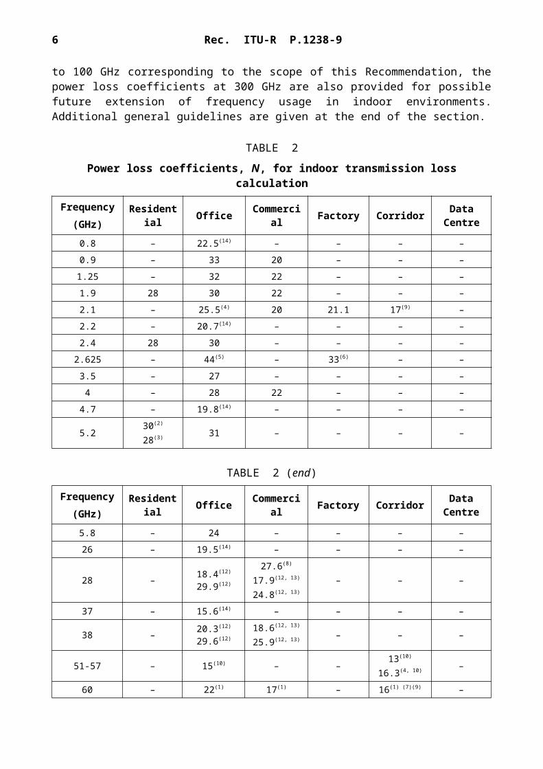
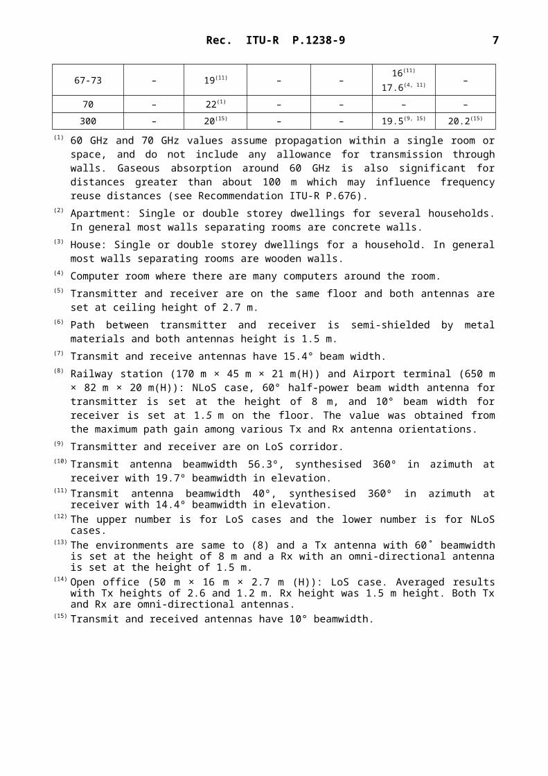
Typical parameters, based on various measurement results, are given in Tables 2 and 3. Although these tables are for mainly up to 100 GHz corresponding to the scope of this Recommendation, the power loss coefficients at 300 GHz are also provided for possible future extension of frequency usage in indoor environments. Additional general guidelines are given at the end of the section.

TABLE 2

Power loss coefficients, N, for indoor transmission loss calculation

Frequency(GHz)

Residential Office Commercial Factory Corridor Data

Centre

0.8 – 22.5(14) – – – –0.9 – 33 20 – – –

1.25 – 32 22 – – –1.9 28 30 22 – – –

2.1 – 25.5(4) 20 21.1 17(9) –2.2 – 20.7(14) – – – –

2.4 28 30 – – – –2.625 – 44(5) – 33(6) – –

3.5 – 27 – – – –4 – 28 22 – – –

4.7 – 19.8(14) – – – –

5.230(2)

28(3) 31 – – – –

Rec. ITU-R P.1238-9 5

TABLE 2 (end)

Frequency(GHz)

Residential Office Commercial Factory Corridor Data

Centre

5.8 – 24 – – – –26 – 19.5(14) – – – –

28 – 18.4(12)

29.9(12)

27.6(8)

17.9(12, 13)

24.8(12, 13)

– – –

37 – 15.6(14) – – – –

38 – 20.3(12)

29.6(12)18.6(12, 13)

25.9(12, 13) – – –

51-57 – 15(10) – –13(10)

16.3(4, 10) –

60 – 22(1) 17(1) – 16(1) (7)(9) –

67-73 – 19(11) – –16(11)

17.6(4, 11) –

70 – 22(1) – – – –

300 – 20(15) – – 19.5(9, 15) 20.2(15)

(1) 60 GHz and 70 GHz values assume propagation within a single room or space, and do not include any allowance for transmission through walls. Gaseous absorption around 60 GHz is also significant for distances greater than about 100 m which may influence frequency reuse distances (see Recommendation ITU-R P.676).

(2) Apartment: Single or double storey dwellings for several households. In general most walls separating rooms are concrete walls.

(3) House: Single or double storey dwellings for a household. In general most walls separating rooms are wooden walls.

(4) Computer room where there are many computers around the room.(5) Transmitter and receiver are on the same floor and both antennas are set at ceiling height of 2.7 m.(6) Path between transmitter and receiver is semi-shielded by metal materials and both antennas height is

1.5 m.(7) Transmit and receive antennas have 15.4° beam width.(8) Railway station (170 m × 45 m × 21 m(H)) and Airport terminal (650 m × 82 m × 20 m(H)): NLoS case,

60° half-power beam width antenna for transmitter is set at the height of 8 m, and 10° beam width for receiver is set at 1.5 m on the floor. The value was obtained from the maximum path gain among various Tx and Rx antenna orientations.

(9) Transmitter and receiver are on LoS corridor.(10) Transmit antenna beamwidth 56.3º, synthesised 360º in azimuth at receiver with 19.7º beamwidth in

elevation.(11) Transmit antenna beamwidth 40º, synthesised 360º in azimuth at receiver with 14.4º beamwidth in

elevation.(12) The upper number is for LoS cases and the lower number is for NLoS cases.(13) The environments are same to (8) and a Tx antenna with 60˚ beamwidth is set at the height of 8 m and a

Rx with an omni-directional antenna is set at the height of 1.5 m.(14) Open office (50 m × 16 m × 2.7 m (H)): LoS case. Averaged results with Tx heights of 2.6 and 1.2 m.

Rx height was 1.5 m height. Both Tx and Rx are omni-directional antennas.(15) Transmit and received antennas have 10° beamwidth.

6 Rec. ITU-R P.1238-9

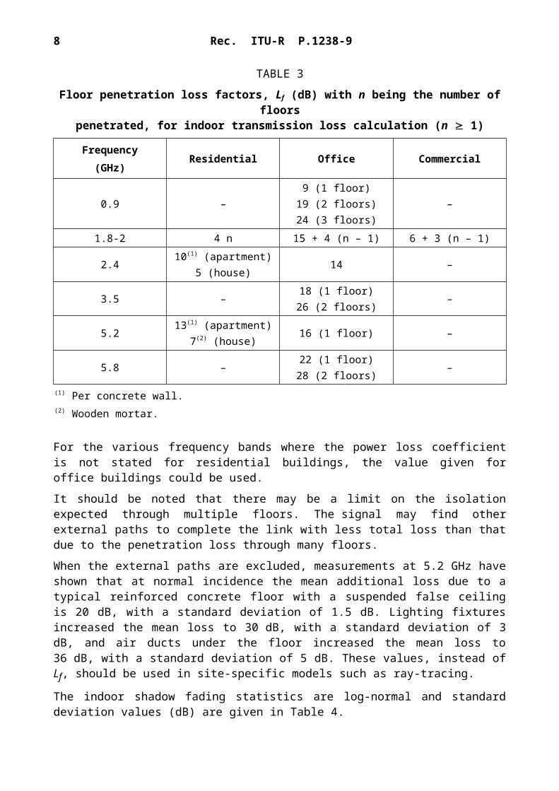
TABLE 3

Floor penetration loss factors, Lf (dB) with n being the number of floorspenetrated, for indoor transmission loss calculation (n 1)

Frequency(GHz)

Residential Office Commercial

0.9 –9 (1 floor)

19 (2 floors)24 (3 floors)

–

1.8-2 4 n 15 + 4 (n – 1) 6 + 3 (n – 1)

2.410(1) (apartment)

5 (house)14 –

3.5 –18 (1 floor)26 (2 floors)

–

5.213(1) (apartment)

7(2) (house)16 (1 floor) –

5.8 –22 (1 floor)28 (2 floors)

–

(1) Per concrete wall.(2) Wooden mortar.

For the various frequency bands where the power loss coefficient is not stated for residential buildings, the value given for office buildings could be used.

It should be noted that there may be a limit on the isolation expected through multiple floors. The signal may find other external paths to complete the link with less total loss than that due to the penetration loss through many floors.

When the external paths are excluded, measurements at 5.2 GHz have shown that at normal incidence the mean additional loss due to a typical reinforced concrete floor with a suspended false ceiling is 20 dB, with a standard deviation of 1.5 dB. Lighting fixtures increased the mean loss to 30 dB, with a standard deviation of 3 dB, and air ducts under the floor increased the mean loss to 36 dB, with a standard deviation of 5 dB. These values, instead of Lf, should be used in site-specific models such as ray-tracing.

The indoor shadow fading statistics are log-normal and standard deviation values (dB) are given in Table 4.

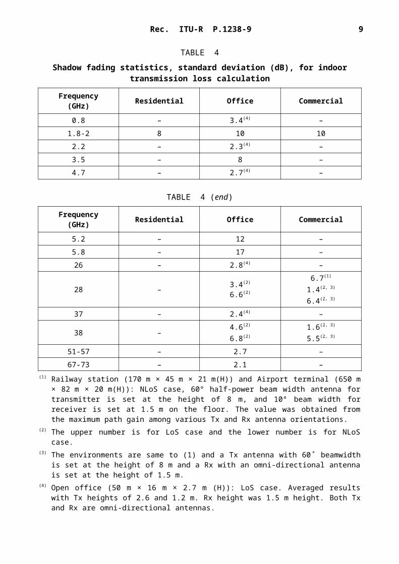
TABLE 4

Shadow fading statistics, standard deviation (dB), for indoor transmission loss calculation

Frequency(GHz) Residential Office Commercial

0.8 – 3.4(4) –1.8-2 8 10 102.2 – 2.3(4) –3.5 – 8 –4.7 – 2.7(4) –

Rec. ITU-R P.1238-9 7

TABLE 4 (end)

Frequency(GHz) Residential Office Commercial

5.2 – 12 –5.8 – 17 –26 – 2.8(4) –

28 – 3.4(2)

6.6(2)

6.7(1)

1.4(2, 3)

6.4(2, 3)

37 – 2.4(4) –

38 –4.6(2)

6.8(2)

1.6(2, 3)

5.5(2, 3)

51-57 – 2.7 –67-73 – 2.1 –

(1) Railway station (170 m × 45 m × 21 m(H)) and Airport terminal (650 m × 82 m × 20 m(H)): NLoS case, 60° half-power beam width antenna for transmitter is set at the height of 8 m, and 10° beam width for receiver is set at 1.5 m on the floor. The value was obtained from the maximum path gain among various Tx and Rx antenna orientations.

(2) The upper number is for LoS case and the lower number is for NLoS case.(3) The environments are same to (1) and a Tx antenna with 60˚ beamwidth is set at the height of 8 m and a

Rx with an omni-directional antenna is set at the height of 1.5 m.(4) Open office (50 m × 16 m × 2.7 m (H)): LoS case. Averaged results with Tx heights of 2.6 and 1.2 m.

Rx height was 1.5 m height. Both Tx and Rx are omni-directional antennas.

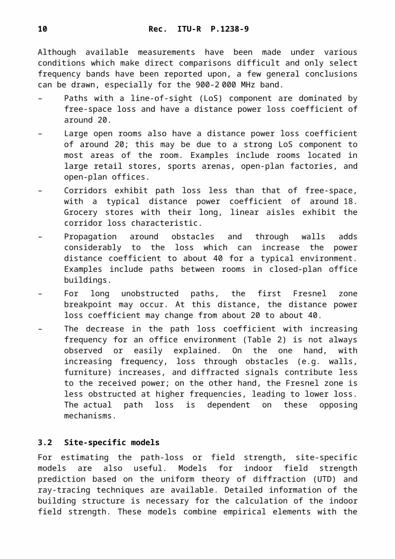
Although available measurements have been made under various conditions which make direct comparisons difficult and only select frequency bands have been reported upon, a few general conclusions can be drawn, especially for the 900-2 000 MHz band.– Paths with a line-of-sight (LoS) component are dominated by free-space loss and have

a distance power loss coefficient of around 20.– Large open rooms also have a distance power loss coefficient of around 20; this may be due

to a strong LoS component to most areas of the room. Examples include rooms located in large retail stores, sports arenas, open-plan factories, and open-plan offices.

– Corridors exhibit path loss less than that of free-space, with a typical distance power coefficient of around 18. Grocery stores with their long, linear aisles exhibit the corridor loss characteristic.

– Propagation around obstacles and through walls adds considerably to the loss which can increase the power distance coefficient to about 40 for a typical environment. Examples include paths between rooms in closed-plan office buildings.

– For long unobstructed paths, the first Fresnel zone breakpoint may occur. At this distance, the distance power loss coefficient may change from about 20 to about 40.

– The decrease in the path loss coefficient with increasing frequency for an office environment (Table 2) is not always observed or easily explained. On the one hand, with increasing frequency, loss through obstacles (e.g. walls, furniture) increases, and diffracted signals contribute less to the received power; on the other hand, the Fresnel zone is less obstructed at higher frequencies, leading to lower loss. The actual path loss is dependent on these opposing mechanisms.

8 Rec. ITU-R P.1238-9

3.2 Site-specific models

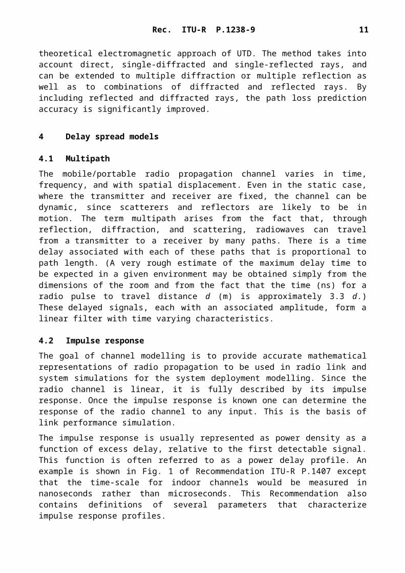
For estimating the path-loss or field strength, site-specific models are also useful. Models for indoor field strength prediction based on the uniform theory of diffraction (UTD) and ray-tracing techniques are available. Detailed information of the building structure is necessary for the calculation of the indoor field strength. These models combine empirical elements with the theoretical electromagnetic approach of UTD. The method takes into account direct, single-diffracted and single-reflected rays, and can be extended to multiple diffraction or multiple reflection as well as to combinations of diffracted and reflected rays. By including reflected and diffracted rays, the path loss prediction accuracy is significantly improved.

4 Delay spread models

4.1 Multipath

The mobile/portable radio propagation channel varies in time, frequency, and with spatial displacement. Even in the static case, where the transmitter and receiver are fixed, the channel can be dynamic, since scatterers and reflectors are likely to be in motion. The term multipath arises from the fact that, through reflection, diffraction, and scattering, radiowaves can travel from a transmitter to a receiver by many paths. There is a time delay associated with each of these paths that is proportional to path length. (A very rough estimate of the maximum delay time to be expected in a given environment may be obtained simply from the dimensions of the room and from the fact that the time (ns) for a radio pulse to travel distance d (m) is approximately 3.3 d.) These delayed signals, each with an associated amplitude, form a linear filter with time varying characteristics.

4.2 Impulse response

The goal of channel modelling is to provide accurate mathematical representations of radio propagation to be used in radio link and system simulations for the system deployment modelling. Since the radio channel is linear, it is fully described by its impulse response. Once the impulse response is known one can determine the response of the radio channel to any input. This is the basis of link performance simulation.

The impulse response is usually represented as power density as a function of excess delay, relative to the first detectable signal. This function is often referred to as a power delay profile. An example is shown in Fig. 1 of Recommendation ITU-R P.1407 except that the time-scale for indoor channels would be measured in nanoseconds rather than microseconds. This Recommendation also contains definitions of several parameters that characterize impulse response profiles.

The channel impulse response varies with the position of the receiver, and may also vary with time. Therefore it is usually measured and reported as an average of profiles measured over one wavelength to reduce noise effects, or over several wavelengths to determine a spatial average. It is important to define clearly which average is meant, and how the averaging was performed. The recommended averaging procedure is to form a statistical model as follows: For each impulse response estimate (power delay profile), locate the times before and after the average delay TD

(see Recommendation ITU-R P.1407) beyond which the power density does not exceed specific values (–10, –15, –20, –25, –30 dB) with respect to the peak power density. The median, and if desired the 90th percentile, of the distributions of these times forms the model.

Rec. ITU-R P.1238-9 9

4.3 r.m.s. delay spread

Power delay profiles are often characterized by one or more parameters, as mentioned above. These parameters should be computed from profiles averaged over an area having the dimensions of several wavelengths. (The parameter r.m.s. delay spread is sometimes found from individual profiles, and the resulting values averaged, but in general the result is not the same as that found from an averaged profile.) A noise exclusion threshold, or acceptance criterion, e.g. 30 dB below the peak of the profile, should be reported along with the resulting delay spread, which depends on this threshold.

Although the r.m.s. delay spread is very widely used, it is not always a sufficient characterization of the delay profile. In multipath environments where the delay spread exceeds the symbol duration, the bit error ratio for phase shift keying modulation depends, not on the r.m.s. delay spread, but rather on the received power ratio of the desired wave to the undesired wave. This is particularly pronounced for high symbol-rate systems, but is also true even at low symbol rates when there is a strong dominant signal among the multipath components (Rician fading).

However, if an exponentially decaying profile can be assumed, it is sufficient to express the r.m.s. delay spread instead of the power delay profile. In this case, the impulse response can be reconstructed approximately as:

h( t )={e– t / S for 0 ≤ t ≤ tmax0 otherwise (2)

where:S : r.m.s. delay spread

tmax : maximum delaytmax  S.

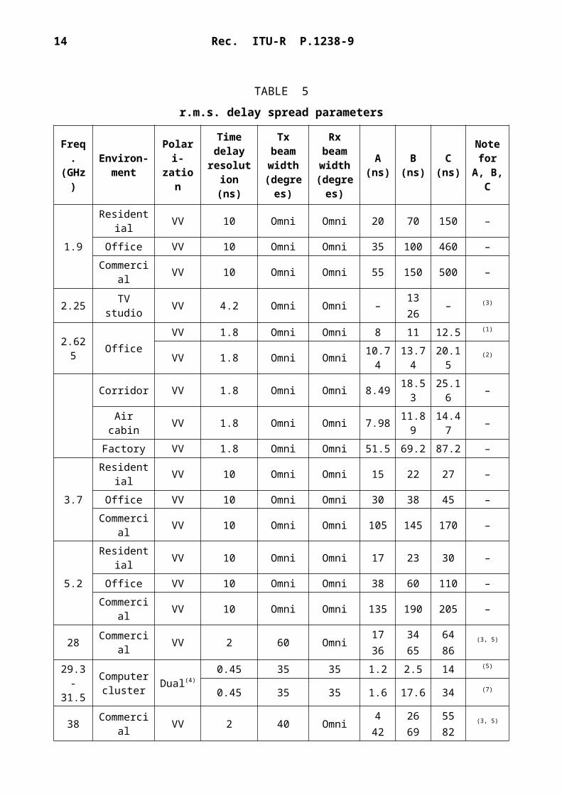
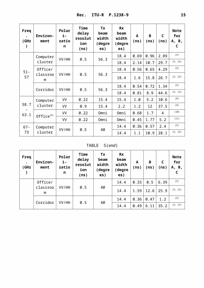
The advantage in using the r.m.s. delay spread as the model output parameter is that the model can be expressed simply in the form of a table. Typical delay spread parameters estimated from averaged delay profiles for indoor environments are given in Table 5. In Table 5, column B represents median values that occur frequently, columns A and C correspond to the 10% and 90% values of the cumulative distribution. The values given in the Table represent the largest room sizes likely to be encountered in each environment.

10 Rec. ITU-R P.1238-9

TABLE 5

r.m.s. delay spread parameters

Freq.(GHz)

Environ-ment

Polari-zation

Timedelay

resolution(ns)

Tx beamwidth

(degrees)

Rx beamwidth

(degrees)

A(ns)

B(ns)

C(ns)

Notefor

A, B, C

1.9Residential VV 10 Omni Omni 20 70 150 –

Office VV 10 Omni Omni 35 100 460 –Commercial VV 10 Omni Omni 55 150 500 –

2.25 TV studio VV 4.2 Omni Omni –1326

– (3)

2.625 OfficeVV 1.8 Omni Omni 8 11 12.5 (1)

VV 1.8 Omni Omni 10.74 13.74 20.15 (2)

Corridor VV 1.8 Omni Omni 8.49 18.53 25.16 –Air cabin VV 1.8 Omni Omni 7.98 11.89 14.47 –Factory VV 1.8 Omni Omni 51.5 69.2 87.2 –

3.7Residential VV 10 Omni Omni 15 22 27 –

Office VV 10 Omni Omni 30 38 45 –Commercial VV 10 Omni Omni 105 145 170 –

5.2Residential VV 10 Omni Omni 17 23 30 –

Office VV 10 Omni Omni 38 60 110 –Commercial VV 10 Omni Omni 135 190 205 –

28 Commercial VV 2 60 Omni1736

3465

6486

(3, 5)

29.3-31.5

Computer cluster Dual(4)

0.45 35 35 1.2 2.5 14 (5)

0.45 35 35 1.6 17.6 34 (7)

38 Commercial VV 2 40 Omni4

422669

5582

(3, 5)

51-57

Computer cluster VV/HH 0.5 56.3

18.4 0.69 0.96 2.89 (5)

18.4 2.14 10.7 29.7 (5, 12)

Office/classroom VV/HH 0.5 56.3

18.4 0.56 0.65 4.29 (5)

18.4 1.6 15.8 26.7 (5, 12)

Corridor VV/HH 0.5 56.318.4 0.54 0.72 1.34 (5)

18.4 0.81 8.9 44.6 (5, 12)

58.7-63.1

Computer cluster

VV 0.22 15.4 15.4 1.0 5.2 10.6 (8)

VV 0.9 15.4 2.2 1.2 12 37.5 (9)

Office(6)VV 0.22 Omni Omni 0.68 1.7 4 (10)

VV 0.22 Omni Omni 0.45 1.77 5.2 (11)

67-73 Computer cluster VV/HH 0.5 40

14.4 0.36 0.57 2.4 (5)

14.4 1.1 10.9 28.1 (5, 12)

Rec. ITU-R P.1238-9 11

TABLE 5(end)

Freq.(GHz)

Environ-ment

Polari-zation

Timedelay

resolution(ns)

Tx beamwidth

(degrees)

Rx beamwidth

(degrees)

A(ns)

B(ns)

C(ns)

Notefor

A, B, C

Office/classroom VV/HH 0.5 40

14.4 0.33 0.5 6.39 (5)

14.4 1.59 12.6 25.9 (5, 12)

Corridor VV/HH 0.5 4014.4 0.36 0.47 1.2 (5)

14.4 0.49 6.11 35.2 (5, 12)

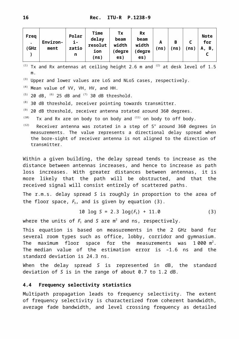
(1) Tx and Rx antennas at ceiling height 2.6 m and (2) at desk level of 1.5 m.(3) Upper and lower values are LoS and NLoS cases, respectively.(4) Mean value of VV, VH, HV, and HH.(5) 20 dB, (6) 25 dB and (7) 30 dB threshold.(8) 30 dB threshold, receiver pointing towards transmitter.(9) 20 dB threshold, receiver antenna rotated around 360 degrees.(10) Tx and Rx are on body to on body and (11) on body to off body.(12) Receiver antenna was rotated in a step of 5o around 360 degrees in measurements. The value represents

a directional delay spread when the bore-sight of receiver antenna is not aligned to the direction of transmitter.

Within a given building, the delay spread tends to increase as the distance between antennas increases, and hence to increase as path loss increases. With greater distances between antennas, it is more likely that the path will be obstructed, and that the received signal will consist entirely of scattered paths.

The r.m.s. delay spread S is roughly in proportion to the area of the floor space, Fs, and is given by equation (3).

10 log S = 2.3 log(Fs) + 11.0 (3)

where the units of Fs and S are m2 and ns, respectively.

This equation is based on measurements in the 2 GHz band for several room types such as office, lobby, corridor and gymnasium. The maximum floor space for the measurements was 1  000 m2. The median value of the estimation error is –1.6 ns and the standard deviation is 24.3 ns.

When the delay spread S is represented in dB, the standard deviation of S is in the range of about 0.7 to 1.2 dB.

4.4 Frequency selectivity statistics

Multipath propagation leads to frequency selectivity. The extent of frequency selectivity is characterized from coherent bandwidth, average fade bandwidth, and level crossing frequency as detailed in Recommendation ITU-R P.1407. Values of the average fade bandwidth that fell below the 6 dB threshold from measurements in indoor environments representative of laboratory and office environment in the 2.38 GHz and in TV studios in the 2.25 GHz band are 27% and 21%, respectively. The corresponding level crossing frequency values are: 0.12 per MHz and 0.24 per MHz.

12 Rec. ITU-R P.1238-9

4.5 Site-specific models

Whilst the statistical models are useful in the derivation of planning guidelines, deterministic (or site-specific) models are of considerable value to those who design the systems. Several deterministic techniques for propagation modelling can be identified. For indoor applications, especially, the finite difference time domain (FDTD) technique and the geometrical optics technique have been studied. The geometrical optics technique is more computationally efficient than the FDTD.

There are two basic approaches in the geometrical optics technique, the image and the ray-launching approach. The image approach makes use of the images of the receiver relative to all the reflecting surfaces of the environment. The coordinates of all the images are calculated and then rays are traced towards these images.

The ray-launching approach involves a number of rays launched uniformly in space around the transmitter antenna. Each ray is traced until it reaches the receiver or its amplitude falls under a specified limit. When compared to the image approach, the ray-launching approach is more flexible, because diffracted and scattered rays can be handled along with the specular reflections. Furthermore, by using the ray-splitting technique or the variation method, computing time can be saved while adequate resolution is maintained. The ray-launching approach is a suitable technique for area-wide prediction of the channel impulse response, while the image approach is suitable for a point-to-point prediction.

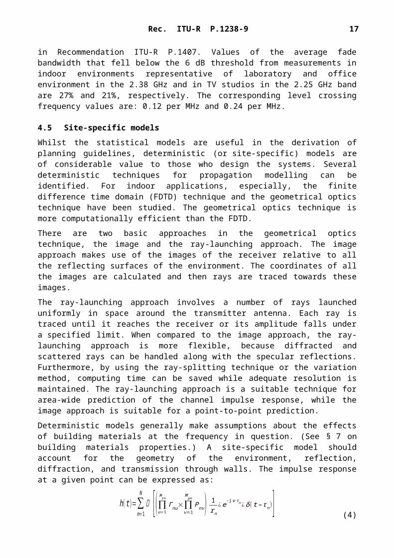
Deterministic models generally make assumptions about the effects of building materials at the frequency in question. (See § 7 on building materials properties.) A site-specific model should account for the geometry of the environment, reflection, diffraction, and transmission through walls. The impulse response at a given point can be expressed as:

h( t )=∑n=1

N

[(∏u=1

Mrn

Γnu×∏v=1

M pn

Pnv) 1rn

¿e–j ω τn¿δ ( t – τ n)]

(4)

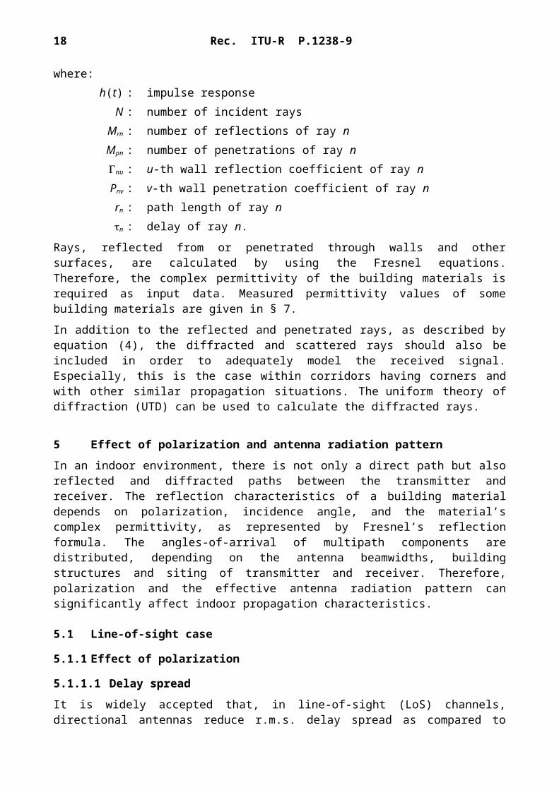
where:h(t) : impulse response

N : number of incident raysMrn : number of reflections of ray nMpn : number of penetrations of ray nnu : u-th wall reflection coefficient of ray nPnv : v-th wall penetration coefficient of ray nrn : path length of ray nn : delay of ray n.

Rays, reflected from or penetrated through walls and other surfaces, are calculated by using the Fresnel equations. Therefore, the complex permittivity of the building materials is required as input data. Measured permittivity values of some building materials are given in § 7.

In addition to the reflected and penetrated rays, as described by equation (4), the diffracted and scattered rays should also be included in order to adequately model the received signal. Especially, this is the case within corridors having corners and with other similar propagation situations. The uniform theory of diffraction (UTD) can be used to calculate the diffracted rays.

Rec. ITU-R P.1238-9 13

5 Effect of polarization and antenna radiation pattern

In an indoor environment, there is not only a direct path but also reflected and diffracted paths between the transmitter and receiver. The reflection characteristics of a building material depends on polarization, incidence angle, and the material’s complex permittivity, as represented by Fresnel’s reflection formula. The angles-of-arrival of multipath components are distributed, depending on the antenna beamwidths, building structures and siting of transmitter and receiver. Therefore, polarization and the effective antenna radiation pattern can significantly affect indoor propagation characteristics.

5.1 Line-of-sight case

5.1.1 Effect of polarization

5.1.1.1 Delay spread

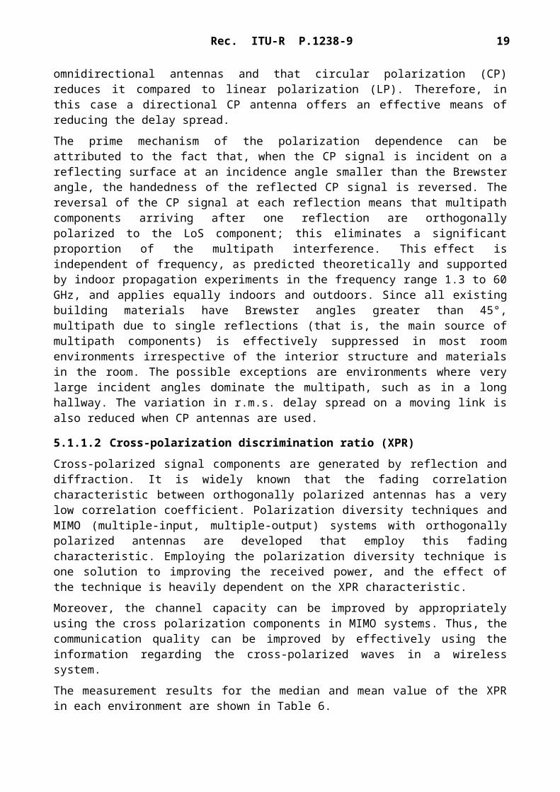
It is widely accepted that, in line-of-sight (LoS) channels, directional antennas reduce r.m.s. delay spread as compared to omnidirectional antennas and that circular polarization (CP) reduces it compared to linear polarization (LP). Therefore, in this case a directional CP antenna offers an effective means of reducing the delay spread.

The prime mechanism of the polarization dependence can be attributed to the fact that, when the CP signal is incident on a reflecting surface at an incidence angle smaller than the Brewster angle, the handedness of the reflected CP signal is reversed. The reversal of the CP signal at each reflection means that multipath components arriving after one reflection are orthogonally polarized to the LoS component; this eliminates a significant proportion of the multipath interference. This effect is independent of frequency, as predicted theoretically and supported by indoor propagation experiments in the frequency range 1.3 to 60 GHz, and applies equally indoors and outdoors. Since all existing building materials have Brewster angles greater than 45°, multipath due to single reflections (that is, the main source of multipath components) is effectively suppressed in most room environments irrespective of the interior structure and materials in the room. The possible exceptions are environments where very large incident angles dominate the multipath, such as in a long hallway. The variation in r.m.s. delay spread on a moving link is also reduced when CP antennas are used.

5.1.1.2 Cross-polarization discrimination ratio (XPR)

Cross-polarized signal components are generated by reflection and diffraction. It is widely known that the fading correlation characteristic between orthogonally polarized antennas has a very low correlation coefficient. Polarization diversity techniques and MIMO (multiple-input, multiple-output) systems with orthogonally polarized antennas are developed that employ this fading characteristic. Employing the polarization diversity technique is one solution to improving the received power, and the effect of the technique is heavily dependent on the XPR characteristic.

Moreover, the channel capacity can be improved by appropriately using the cross polarization components in MIMO systems. Thus, the communication quality can be improved by effectively using the information regarding the cross-polarized waves in a wireless system.

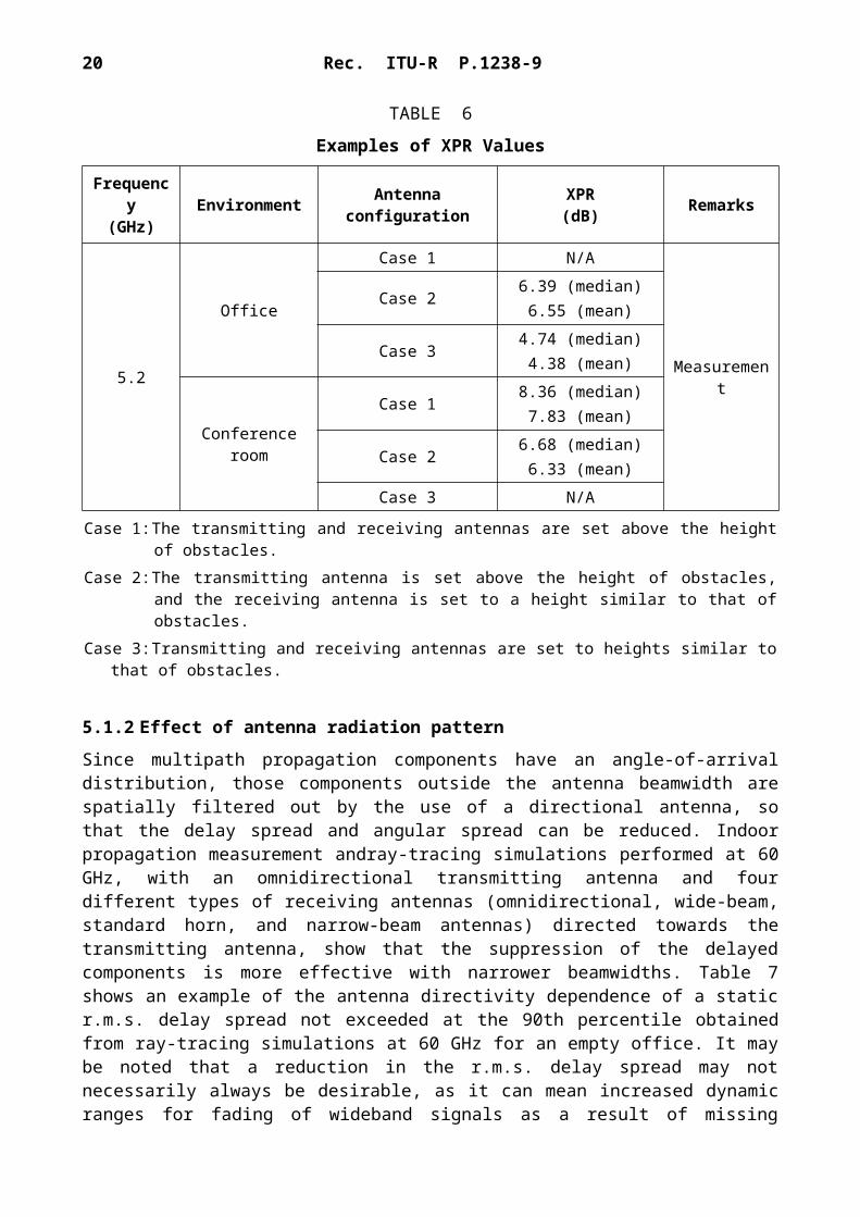
The measurement results for the median and mean value of the XPR in each environment are shown in Table 6.

14 Rec. ITU-R P.1238-9

TABLE 6

Examples of XPR Values

Frequency(GHz) Environment Antenna configuration XPR

(dB) Remarks

5.2

Office

Case 1 N/A

Measurement

Case 26.39 (median)6.55 (mean)

Case 34.74 (median)4.38 (mean)

Conference room

Case 18.36 (median)7.83 (mean)

Case 26.68 (median)6.33 (mean)

Case 3 N/A

Case 1: The transmitting and receiving antennas are set above the height of obstacles.Case 2: The transmitting antenna is set above the height of obstacles, and the receiving antenna is set to a

height similar to that of obstacles.Case 3: Transmitting and receiving antennas are set to heights similar to that of obstacles.

5.1.2 Effect of antenna radiation pattern

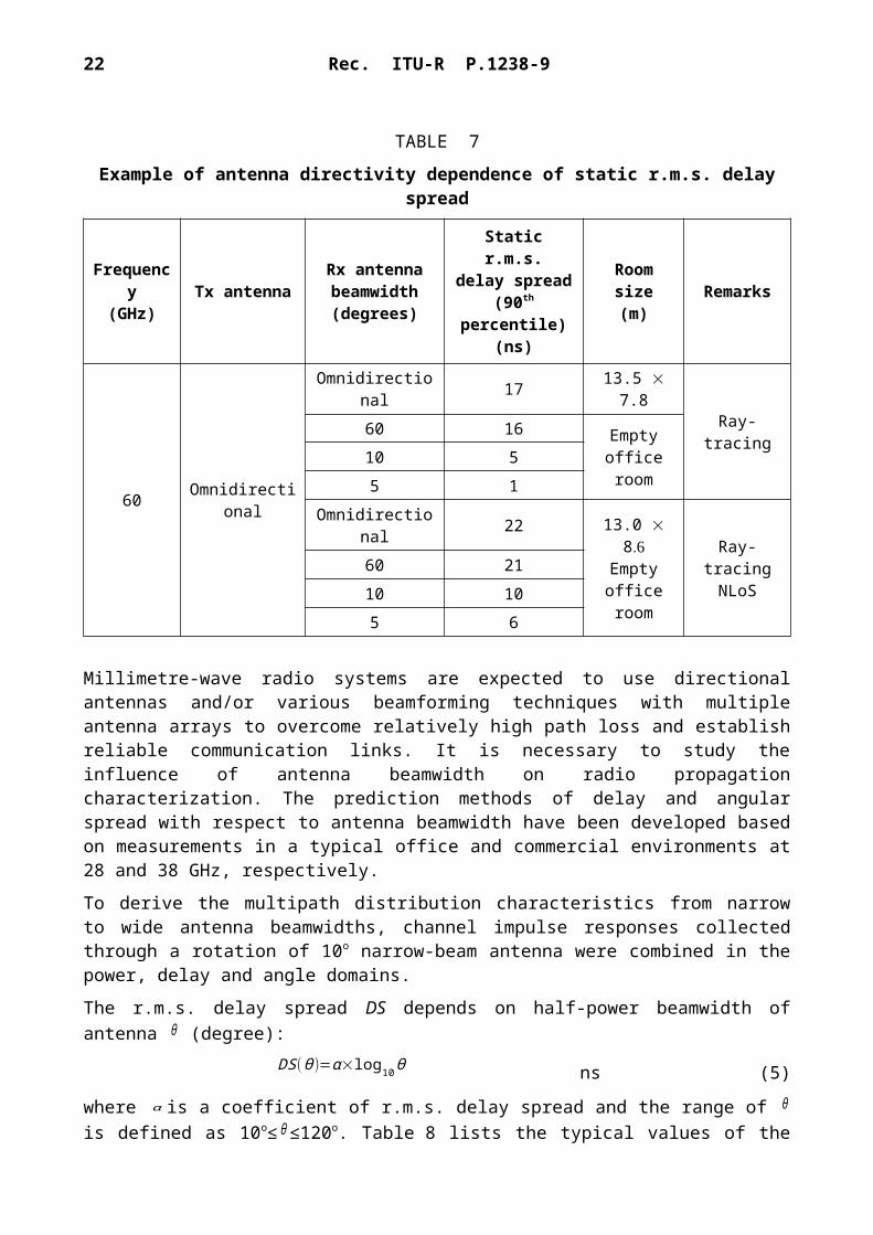
Since multipath propagation components have an angle-of-arrival distribution, those components outside the antenna beamwidth are spatially filtered out by the use of a directional antenna, so that the delay spread and angular spread can be reduced. Indoor propagation measurement andray-tracing simulations performed at 60 GHz, with an omnidirectional transmitting antenna and four different types of receiving antennas (omnidirectional, wide-beam, standard horn, and narrow-beam antennas) directed towards the transmitting antenna, show that the suppression of the delayed components is more effective with narrower beamwidths. Table 7 shows an example of the antenna directivity dependence of a static r.m.s. delay spread not exceeded at the 90th percentile obtained from ray-tracing simulations at 60 GHz for an empty office. It may be noted that a reduction in the r.m.s. delay spread may not necessarily always be desirable, as it can mean increased dynamic ranges for fading of wideband signals as a result of missing inherent frequency diversity. In addition, it may be noted that some transmission schemes take advantage of multipath effects.

Rec. ITU-R P.1238-9 15

TABLE 7

Example of antenna directivity dependence of static r.m.s. delay spread

Frequency(GHz) Tx antenna

Rx antennabeamwidth(degrees)

Static r.m.s.delay spread

(90th percentile)(ns)

Room size(m) Remarks

60 Omnidirectional

Omnidirectional 17 13.5 7.8

Ray-tracing60 16

Empty office room10 5

5 1Omnidirectional 22

13.0  8Empty office

room

Ray-tracingNLoS

60 2110 105 6

Millimetre-wave radio systems are expected to use directional antennas and/or various beamforming techniques with multiple antenna arrays to overcome relatively high path loss and establish reliable communication links. It is necessary to study the influence of antenna beamwidth on radio propagation characterization. The prediction methods of delay and angular spread with respect to antenna beamwidth have been developed based on measurements in a typical office and commercial environments at 28 and 38 GHz, respectively.

To derive the multipath distribution characteristics from narrow to wide antenna beamwidths, channel impulse responses collected through a rotation of 10o narrow-beam antenna were combined in the power, delay and angle domains.

The r.m.s. delay spread DS depends on half-power beamwidth of antenna θ (degree):

DS(θ )=α× log10θ                 ns (5)

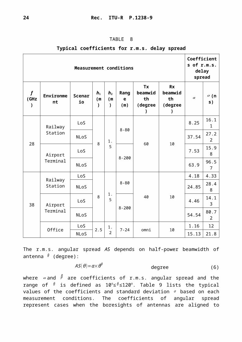
where α is a coefficient of r.m.s. delay spread and the range of θ is defined as 10o≤θ ≤120o. Table 8 lists the typical values of the coefficients and a standard deviation σ based on each measurement conditions. The coefficients of delay spread represent cases when the boresights of antennas were aligned to have maximum receiving power in LoS and NLoS situations, respectively.

16 Rec. ITU-R P.1238-9

TABLE 8

Typical coefficients for r.m.s. delay spread

Measurement conditionsCoefficients of

r.m.s. delay spread

f(GHz) Environment Scenario h1

(m)h2

(m)Range

(m)

Tx beamwidt

h(degree)

Rx beamwidth

(degree)

α σ(ns)

28

Railway Station

LoS

8 1.5

8-80

60 10

8.25 16.11

NLoS 37.54 27.22

Airport Terminal

LoS8-200

7.53 15.98

NLoS 63.9 96.57

38

Railway Station

LoS

8 1.5

8-80

40 10

4.18 4.33NLoS 24.85 28.48

Airport Terminal

LoS8-200

4.46 14.13NLoS 54.54 80.72

OfficeLoS

2.5 1.2 7-24 omni 101.16 12

NLoS 15.13 21.8

The r.m.s. angular spread AS depends on half-power beamwidth of antenna θ (degree):

AS(θ )=α×θβ                degree (6)

where α and β are coefficients of r.m.s. angular spread and the range of θ is defined as 10o≤θ≤120o. Table 9 lists the typical values of the coefficients and standard deviation σ based on each measurement conditions. The coefficients of angular spread represent cases when the boresights of antennas are aligned to have maximum receiving power in LoS and NLoS situations, respectively.

Rec. ITU-R P.1238-9 17

TABLE 9

Typical coefficients for r.m.s. angular spread

Measurement conditions Coefficients of r.m.s. angular spread

f(GHz) Environment Scenario h1

(m)h2

(m)Range

(m)

Tx beam-width

(degree)

Rx beam-width

(degree)

α β σ(degree)

28

Railway Station

LoS

8 1.5

8-80

60 10

0.5 0.77 2.3

NLoS 0.25 1.0 2.32

Airport Terminal

LoS8-200

1.2 0.49 2.18

NLoS 0.3 0.96 3.12

38

Railway Station

LoS

8 1.58-80

40 10

1.14 0.54 3.36NLoS 0.16 1.1 3.24

Airport Terminal

LoS8-200

2.0 0.34 1.36NLoS 0.34 0.93 2.99

OfficeLoS

2.5 1.2 7-24 omni 100.07 1.22 5.58

NLoS 0.17 1.07 4.81

5.2 Obstructed path case

When the direct path is obstructed, the polarization and antenna directivity dependence of the delay spread may be more complicated than those in the LoS path. There are few experimental results relating to the obstructed case. However, an experimental result obtained at 2.4 GHz suggests that the polarization and antenna directivity dependence of the delay spread in the obstructed path is significantly different from that in the LoS path. For instance, an omnidirectional horizontally polarized antenna at the transmitter and a directional CP receiving antenna gave the smallest r.m.s. delay spread and lowest maximum excess delay in the obstructed path.

5.3 Orientation of mobile terminal

In the portable radio environment, propagation is generally dominated by reflection and scattering of the signal. Energy is often scattered from the transmitted polarization into the orthogonal polarizations. Under these conditions, cross-polarization coupling increases the probability of adequate received levels of randomly oriented portable radios. Measurement of cross-polarization coupling carried out at 816 MHz showed a high degree of coupling.

6 Effect of transmitter and receiver siting

There are few experimental and theoretical investigations regarding the effect of transmitter and receiver site on indoor propagation characteristics. In general, however, it may be suggested that the base station should be placed as high as possible near the room ceiling to attain LoS paths as far as possible. In the case of hand-held terminals, the user terminal position will of course be dependent on the user’s motion rather than any system design constraints.

18 Rec. ITU-R P.1238-9

However, for non-hand-held terminals, it is suggested that the antenna height be sufficient to ensure LoS to the base station whenever possible. The choice of station siting is also very relevant to system configuration aspects such as spatial diversity arrangements, zone configuration, etc.

7 Effect of building materials, furnishings and furniture

Indoor propagation characteristics are affected by reflection from and transmission through the building materials. The reflection and transmission characteristics of those materials depend on the complex permittivity of the materials. Site-specific propagation prediction models may need information on the complex permittivity of building materials and on building structures as basic input data, and such information is given in Recommendation ITU-R P.2040.

Specular reflections from floor materials such as floorboard and concrete plate are significantly reduced in millimetre-wave bands when materials are covered by carpet with rough surfaces. Similar reductions may occur with window coverings such as draperies. Therefore, it is expected that the particular effects of materials would be more important as frequency increases.

In addition to the fundamental building structures, furniture and other fixtures also significantly affect indoor propagation characteristics. These may be treated as obstructions and are covered in the path loss model in § 3.

8 Effect of movement of objects in the room

The movement of persons and objects within the room cause temporal variations of the indoor propagation characteristics. This variation, however, is very slow compared to the data rate likely to be used, and can therefore be treated as virtually a time-invariant random variable. Apart from people in the vicinity of the antennas or in the direct path, the movement of persons in offices and other locations in and around the building has a negligible effect on the propagation characteristics.

Measurements performed when both of the link terminals are fixed indicate that fading is bursty (statistics are very non-stationary), and is caused either by the perturbation of multipath signals in areas surrounding a given link, or by shadowing due to people passing through the link.

Measurements at 1.7 GHz indicate that a person moving into the path of a LoS signal causes a 6 to 8 dB drop in received power level, and the K-value of the Nakagami-Rice distribution is considerably reduced. In the case of non-LoS conditions, people moving near the antennas did not have any significant effects on the channel.

In the case of a hand-held terminal, the proximity of the user’s head and body affect the received signal level. At 900 MHz with a dipole antenna, measurements show that received signal strength decreased by 4 to 7 dB when the terminal was held at the waist, and 1 to 2 dB when the terminal was held against the head of the user, in comparison to received signal strength when the antenna was several wavelengths away from the body.

When the antenna height is lower than about 1 m, for example, in the case of a typical desktop or laptop computer application, the LoS path may be shadowed by people moving in the vicinity of the user terminal. For such data applications, both the depth and the duration of fades are of interest. Measurements at 37 GHz in an indoor office lobby environment have shown that fades of 10 to 15 dB were often observed. The duration of these fades due to body shadowing, with people moving continuously in a random manner through the LoS, follows a log-normal distribution, with the mean and standard deviation dependent on fade depth. For these measurements, at a fade depth of 10 dB, the mean duration was 0.11 s and the standard deviation was 0.47 s. At a fade depth of 15 dB, the mean duration was 0.05 s and the standard deviation was 0.15 s.

Rec. ITU-R P.1238-9 19

Measurements at 70 GHz have shown that the mean fade duration due to body shadowing were 0.52 s, 0.25 s and 0.09 s for the fade depth of 10 dB, 20 dB and 30 dB, respectively, in which the mean walking speed of persons was estimated at 0.74 m/s with random directions and human body thickness was assumed to be 0.3 m.

Measurements indicate that the mean number occurrence of body shadowing in an hour caused by human movement in an office environment is given by:

N=260 × D p (7)

where Dp (0.05 < Dp < 0.08) is the number of persons per square metre in the room. Then the total fade duration per hour is given by:

T= T s × N(8)

where T s is mean fade duration.

The number of occurrences of body shadowing in an hour at the passage in an exhibition hall was 180 to 280, where Dp was 0.09 to 0.13.

The distance dependency of path loss in an underground mall is affected by human body shadowing. The path loss in an underground mall is estimated by the following equation with the parameters given in Table 10.

L( x )=−10⋅α {1. 4 − log10( f )− log10( x )} + δ⋅x + C                 dB (9)

where:f: frequency (MHz)x: distance (m).

Parameters for the non-line-of-sight (NLoS) case are verified in the 5 GHz band and those of the LoS case are applicable to the frequency range of 2 GHz to 20 GHz. The range of distance x is 10 m to 200 m.

The environment of the underground mall is a ladder type mall that consists of straight corridors with glass or concrete walls. The main corridor is 6 m wide, 3 m high, and 190 m long. The typical human body is considered to be 170 cm tall and 45 cm wide shoulders. The densities of passers-by are approximately 0.008 persons/m2 and 0.1 persons/m2 for a quiet period (early morning, off-hour) and a crowded period (lunchtime or rush-hour), respectively.

TABLE 10

Parameters for modelled path loss function in Yaesu underground mall

LoS NLoS

δ(m−1)

C(dB)

δ(m−1)

C(dB)

Off-hour 2.0 0 –5 3.4 0 −45Rush-hour 2.0 0.065 –5 3.4 0.065 −45

20 Rec. ITU-R P.1238-9

9 Angular spread models

9.1 Cluster model

In a propagation model for broadband systems using array antennas, a cluster model combining both temporal and angular distributions is applicable. The cluster comprises scattered waves arriving at the receiver within a limited time and angle as shown in Fig. 1. Temporal delay characteristics are found in § 4 of this Recommendation. The distribution of cluster arrival angle i

based on the reference angle (which may be chosen arbitrarily) for an indoor environment is approximately expressed by a uniform distribution on [0, 2.

FIGURE 1Image of cluster model

9.2 Angular distribution of arrival waves from within i-th cluster

The probability density function of the angular distribution of arrival waves within a cluster is expressed by:

Pi (ϕ−Θi )=1

√2 σ i

⋅exp (−√2|ϕ−Θi|

σ i)

(10)

where is the angle of arrival of arriving waves within a cluster in degrees referencing to the reference angle and i is the standard deviation of the angular spread in degrees.

The angular spread parameters in an indoor environment are given in Table 11.

Rec. ITU-R P.1238-9 21

TABLE 11

Angular spread parameters in indoor environment

LoS NLoS

Mean (degrees) Range (degrees) Mean (degrees) Range (degrees)

Hall 23.7 21.8-25.6 – –Office 14.8 3.93-28.8 54.0 54Home 21.4 6.89-36 25.5 4.27-46.8

Corridor 5 5 14.76 2-37

9.3 Double directional angular spread

In a propagation model for broadband communication with multiple antenna arrays at the transmitter and receiver, the angular distribution at the transmitting and at the receiving stations is applicable. From measurements with 240 MHz bandwidth at 2.38 GHz, the mean RMS angular spread in an indoor corridor and office environment for 20 dB threshold level are given in Table 12.

TABLE 12

Double directional angular spread

Station 1 height(m)

RMS angular spread at station 1

(degrees)

Station 2 height(m)

RMS angular spread at station 2

(degrees)

Corridor and office 1.9 68.5 1.7 69.7

10 Statistical model in static usage

When wireless terminals such as cellular phones and WLANs are used indoors, they are basically static. In static usage, the wireless terminal itself does not move, but the environment around it changes due to the movement of blocking objects such as people. In order to accurately evaluate the communication quality in such an environment, we provide a channel model for static indoor conditions, which gives the statistical characteristics of both the probability density function (PDF) and autocorrelation function of received level variation at the same time.

The channel models for indoor NLoS and LoS environments are discussed.

10.1 DefinitionNperson: number of moving people

w: equivalent diameter of moving person (m)v: moving speed of people (m/s)

Pm: total multipath’s powerS(x,y): layout of moving area

fT : maximum frequency shift for static mobile terminalrp: received power at the mobile terminal

22 Rec. ITU-R P.1238-9

f: frequency (Hz)p(rp,k): probability density function (PDF) of received power defined as Nakagami-

Rice distribution with K-factorK: K-factor defined in the Nakagami-Rice distribution

R(t): autocorrelation function of received levelRN(t): autocorrelation coefficient of received level

P(f): power spectrumPN(f): power spectrum normalized by power P(0).

10.2 System model

Figure 2 shows the system model. The moving objects considered are only people; the i th person is represented as a disk with a diameter of w (m) separated from the mobile terminal (MT) by ri(m). Each moving person walks in an arbitrary direction between 0 and 2 at a constant speed of v (m/s) and moves within an arbitrary area S(x,y) around the MT. The number of moving people is Nperson

and a moving person absorbs a part of the energy of the paths that cross his width, w. The multipaths arrive at the terminal uniformly from all horizontal directions. Figures 3 and 4 show the typical rooms considered, rectangular and circular, respectively.

FIGURE 2System model

FIGURE 3Rectangular-shaped room layout

Rec. ITU-R P.1238-9 23

FIGURE 4Circular-shaped room layout

10.2.1 Probability density function of received power

The PDF of received power rp at the mobile terminal is given by the Nakagami-Rice distribution as follows.

p (r P , K ) = (K + 1 ) exp [−( K + 1 )r P − K ] I0 (√4 ( K + 1 ) KrP ) (11)

where I0(x) is the first kind 0th-order modified Bessel function and K represents the following K-factor.

K ≡ K ( x ) =|e Direct ( x ) + es ( x )|2 / ( N person Pm ΔwSShape

2 π )(12)

where:

S Shape = ¿¿¿¿ (13)

Here eDirect(x) represents the complex envelop of the direct path and es(x) represents the complex envelop of multipaths without moving objects around the MT at the position of x, which depends on only the surrounding static environment; their values do not depend on time t. Pm represents total multipath power. SShape is a constant value determined by the room’s shape and dimensions.

10.2.2 Autocorrelation function of received signal level

The autocorrelation function R(t) of the received complex signal level with time difference t is given as follows:

24 Rec. ITU-R P.1238-9

R(Δt )= ¿{Pm (|eDirect ( x ) + es ( x )|2

Pm+

N person ΔwSShape

2 π (1 –2 f T|Δt|π )) (v|Δt|≤ Δw ) ¿ {¿ {Pm [|eDirect ( x ) + es ( x )|2

Pm+

N person Δ wSShape

2π {1 –2 f T|Δt|π

– 2π

cos– 1 (1f T |Δt| ) + 2 f T |Δt|π

sin (cos– 1(1f T |Δt|))}] ¿ ¿¿

¿

¿

(14)

where:

f T = v /Δw (15)

Here fT is determined by the moving speed v and the width w of moving people and can be considered as the maximum frequency shift for the static mobile terminal.

10.2.3 Power spectrum of received signal

Power spectrum P(f ) as a function of frequency, which determines the variation of the complex envelop, is given by the Fourier transform of the autocorrelation function R(t) in equation (14) as follows.

P( f ) =∫–∞

∞R( Δt ) e– j2 πfΔτ dΔt

(16)

The power spectrum PN(f ), which is normalized by power P(0) at the frequency of f = 0 Hz, can be approximated as follows.

PN ( f ) = P ( f ) / P (0)

¿ ( K ( x ) δ ( f ) ¿ )¿¿

¿¿¿¿(17)

Here (f ) represents Dirac’s delta function.

10.2.4 Values

w is recommended to be set at 0.3 m as representative of an average adult man.

10.2.5 Examples

When w, v and Nperson are 0.3 m, 1 m/s, and 10, respectively, and rmax is set to 10 m for the circular room, the PDF p(rp, K(x)), autocorrelation function RN(t) and power spectrum PN(f ) by using equations (11), (12) and (17) are as shown in Figs 5, 6 and 7, respectively.

Rec. ITU-R P.1238-9 25

FIGURE 5Cumulative probability of received level in circular room

FIGURE 6Autocorrelation coefficient of received level in circular room

26 Rec. ITU-R P.1238-9

FIGURE 7Power spectrum in circular room