MSU International Development

Working Paper 157 October 2017

Does Farm Structure Matter? The Effects of Farmland Distribution Patterns on Rural Household Incomes in Tanzania by

Jordan Chamberlin and T. S. Jayne

Department of Agricultural, Food, and Resource Economics Department of Economics

MICHIGAN STATE UNIVERSITY East Lansing, Michigan 48824

MSU Agricultural, Food, and Resource Economics Web Site: http://www.canr.msu.edu/afre/

MSU Food Security Group Web Site: https://www.canr.msu.edu/fsg/index MSU is an affirmative-action, equal-opportunity employer

MSU International Development Working Paper

MSU INTERNATIONAL DEVELOPMENT PAPERS

The Michigan State University (MSU) International Development Paper series is designed to further the comparative analysis of international development activities in Africa, Latin America, Asia, and the Near East. The papers report research findings on historical, as well as contemporary, international development problems. The series includes papers on a wide range of topics, such as alternative rural development strategies; nonfarm employment and small scale industry; housing and construction; farming and marketing systems; food and nutrition policy analysis; economics of rice production in West Africa; technological change, employment, and income distribution; computer techniques for farm and marketing surveys; farming systems and food security research. The papers are aimed at teachers, researchers, policy makers, donor agencies, and international development practitioners. Selected papers will be translated into French, Spanish, or other languages.

Copies of all MSU International Development Papers, Working Papers, and Policy Syntheses are freely downloadable in pdf format from the following Web sites:

MSU International Development Papers http://wayback.archive-it.org/org-413/20171227150238/http://fsg.afre.msu.edu/papers/idp.htm http://ideas.repec.org/s/ags/mididp.html

MSU International Development Working Papers

https://www.canr.msu.edu/fsg/publications/idwp%202 http://ideas.repec.org/s/ags/midiwp.html MSU International Development Policy Syntheses https://www.canr.msu.edu/fsg/publications/policy-synthesis-2 http://ideas.repec.org/s/ags/midips.html

Copies of all MSU International Development publications are also submitted to the USAID Development Experience Clearing House (DEC) at: https://dec.usaid.gov/dec/home/

DOES FARM STRUCTURE MATTER? THE EFFECTS OF FARMLAND DISTRIBUTION PATTERNS ON RURAL HOUSEHOLD

INCOMES IN TANZANIA

by

Jordan Chamberlin and T. S. Jayne

October 2017

Chamberlin is Spatial Economist – Socioeconomics Program, International Maize and Wheat Improvement Center (CIMMYT) and Jayne is University Foundation Professor, Michigan State University.

ii

ISSN 0731-3483

© All rights reserved by Michigan State University, 2017

Michigan State University agrees to and does hereby grant to the United States Government a royalty-free, non-exclusive and irrevocable license throughout the world to use, duplicate, disclose, or dispose of this publication in any manner and for any purposes and to permit others to do so.

Published by the Department of Agricultural, Food, and Resource Economics and the Department of Economics, Michigan State University, East Lansing, Michigan 48824-1039, U.S.A.

iii

ACKNOWLEDGMENTS

The authors gratefully acknowledge financial support from the Feed the Future Innovation Lab for Food Security Policy (Cooperative Agreement AID-OAA-L-13-00001 between Michigan State University and the USAID Bureau for Food Security, Office of Agriculture, Research, and Technology), and from the Guiding Investments in Sustainable Agricultural Intensification in Africa (GISAIA) grant from the Bill and Melinda Gates Foundation.

The authors acknowledge helpful comments received from Andrew Dillon, Robert Myers, Felix Kwame Yeboah, Milu Muyanga, Ayala Wineman, and participants at the PEGNet Conference, Zurich, Switzerland, September 14, 2017. The authors are also most grateful to Patricia Johannes for editing and formatting assistance.

Any errors are our own.

iv

EXECUTIVE SUMMARY

This study attempts to evaluate the impacts of localized measures of farm structure (i.e., the local distribution of farm sizes) on smallholder household incomes in Tanzania. Based on the pioneering structural transformation work of Mellor, Johnston and others, the distribution of productive assets in primarily agrarian areas might influence the strength of agricultural growth multiplier effects on both farm and off-farm economic activity and hence on household incomes. Land is the most important productive non-labor asset in rural areas of Sub-Saharan Africa, and many measures of farm structure may be conceptually related to access to land; for example, we may speak of farmland concentration in cases where relatively few farms have relatively large shares of the arable land resources in a given area. If a relatively small set of large farms dominates production, then growth multipliers may be lower than for areas with more egalitarian land distributions. If, on the other hand, large farms bring benefits that spill over to surrounding smallholders, then we might expect positive impacts of more heterogeneous farm size mixtures on household incomes.

The question of whether or not the local structure of land ownership matters for rural growth is important for several reasons, particularly within the African context. First, changes in farm structure are occurring rapidly in many Sub-Saharan African countries, with a major trend being one of increasing land concentration driven by medium- and large-scale land acquisitions in customary tenure systems (Jayne et al. 2003, 2014, 2016; Sitko and Chamberlin 2016; Anseeuw et al. 2016). These studies suggest a de facto move towards greater concentration, under existing land policies. No other research to date, however, has investigated what these changes in agrarian structure imply for rural development outcomes, such as household income per full-time-equivalent (FTE) unit of labor.

To investigate this relationship, we assemble a variety of household- and district-level variables for rural Tanzania, using data from multiple datasets. We use data on farm household income, demographic characteristics, assets and other household-level controls from the 2009, 2011, and 2012 rounds of the Tanzanian Living Standards Measurement Survey – Integrated Survey of Agriculture (LSMS-ISA). We also assemble a variety of farm structure measures for rural Tanzania at the district level, based on the 2009 Agricultural Sample Census, which provides a more comprehensive accounting of farms of all sizes than does the LSMS data. Because farm structure is a multifaceted concept, five alternative indicators of farm structure are used in the analysis, including (i) the Gini coefficient; (ii) skewness; (iii) coefficient of variation; (iv) share of controlled farmland under medium-scale farms; and (v) share of controlled farmland under large farms.

Key Findings

We show that alternative indicators of farm structure differ considerably from one another. Some indicators emphasize the relative importance of different scales of farm operations in the locality, while others focus on the degree to which farmland operations are concentrated or unequally distributed. These observations reinforce a point that should already be well accepted—that farm or agrarian structure is a multifaceted concept and that specific indicators of agrarian structure may not be highly correlated with one another. For this reason, evaluation of the impacts of different farm structures is likely to be sensitive to the choice of indicator used in analysis.

Taking account of this heterogeneity of measurement options, our study produces four main findings. First, heterogeneous localized farm size distributions are generally positively associated with rural household incomes, after controlling for other geographical and

v

household-level factors. Second, household incomes from farm, agricultural wage and non-farm sources are particularly positively and significantly associated with the share of land in the district under farms of 5-10 hectares (which we refer to in this paper as medium-scale farms). Third, these positive spillover benefits are smaller and less statistically significant in districts with a relatively high share of farmland under farms over 10 hectares in size. While our econometric results do not identify the reason why medium-scale farms appear to generate greater spillover effects to local communities than relatively large farms, recent published studies give us some clues – most medium-scale farmers come from the same social and ethnic backgrounds as small-scale farmers, and tend to have more extensive social interactions with the local community than do most large-scale farms (Sitko and Jayne 2014). Fourth, poor rural households are least able to capture the positive spillovers generated by medium-scale farms and by concentrated farmland patterns. The greatest benefits to household income were enjoyed by households in the upper two-thirds of the wealth distribution, which still includes the majority of rural households. We speculate that poor rural households are less able to afford taking advantage of the improved access to markets and services that medium-scale farms tend to provide. However, more detailed research is needed on the pathways by which medium- and large-scale farms affect household and broader local community welfare. Conclusion and Recommendations

Our study suggests that relatively heterogeneous agrarian structures confer positive benefits on smallholder welfare outcomes. However, this is not unambiguously true: concentration of land under the largest farms in our sample (>10 ha) is not positively associated with smallholder incomes, suggesting that most of the benefits of land concentration come from farms in 5-10 hectare range. We suggest that more empirical research be undertaken to (a) determine whether or not these relationships are found in other countries, and (b) uncover the specific mechanisms by which larger farms may provide spillover benefits to nearby smaller farms within the same areas. A better understanding of the latter in particular will help to clarify what kinds of farms, in terms of size and nature of operations, are associated with the largest positive multiplier effects. We believe this is a fundamentally important area for further research investments, given the rapid growth in farmland acquisitions by medium and large farming enterprises in much of the region.

Our research underscores the importance of accurate data to understanding processes of economic development and to identifying strategies that can promote income growth and living standards. The relatively recent bounty of nationally representative data available through such initiatives as the World Bank’s LSMS-ISA program is certainly to be applauded. Nonetheless, we would advocate for even greater investments in expanding the sampling frame – both to ensure adequate representation of larger farms, as well as to enable more spatially disaggregated measures of farm structure and land access. Although this will require increased investments in data collection, the payoffs are likely to be substantial, particularly in countries where medium- and large-scale land acquisitions are clearly taking place. Because many of these acquisitions are taking place under the radar of traditional data collection mechanisms, and in some cases may be transforming rural farm structure quite rapidly, it is important to plan for such investments now. Unfortunately, discussions of land policy and agricultural policy in SSA remain largely disconnected. Ultimately, the scope for African states to rationally guide how land access contributes (or not) to rural development will depend upon how well we are able to monitor and evaluate the changes taking place on the ground.

vi

CONTENTS

ACKNOWLEDGMENTS ........................................................................................................ iii EXECUTIVE SUMMARY ...................................................................................................... iv

LIST OF TABLES ................................................................................................................... vii LIST OF FIGURES ................................................................................................................ viii ACRONYMS .......................................................................................................................... viii 1. INTRODUCTION ................................................................................................................. 1

2. CONCEPTUAL FRAMEWORK .......................................................................................... 3

2.1. Core Theoretical Perspectives ......................................................................................... 3

2.2. Model of Per-Full Time Equivalent Gross Income Determinants .................................. 4

3. DATA AND VARIABLE CONSTRUCTION ..................................................................... 6

3.1. Data Sources ................................................................................................................... 6

3.2. Variable Construction ..................................................................................................... 6

3.1.1. Variables Measuring Farm Structure and Land Concentration ............................... 7

3.1.2. Outcome Variables................................................................................................... 8

3.1.3. Full-time Equivalents ............................................................................................... 8

4. IMPLEMENTATION CHALLENGES................................................................................. 9

4.1. Data Quality Issues ......................................................................................................... 9

4.2. Endogeneity Concerns .................................................................................................... 9

4.3. Attrition ......................................................................................................................... 10

5. DESCRIPTIVE RESULTS .................................................................................................. 11

5.1. Farm Size Structure....................................................................................................... 11

5.2. Income Trends, by Farm Size Category ....................................................................... 11

5.3. Land Concentration Measures ...................................................................................... 12

6. ECONOMETRIC ANALYSIS ........................................................................................... 15

6.1. Baseline Specification ..................................................................................................... 15

6.2. Interacting Concentration with Household Asset Dummies ......................................... 18

6.3. Inter-Period Income Changes Regressed on Lagged Independent Variables ............... 19

6.4. Simulated Impacts of Changes in Density ....................................................................... 20

7. CONCLUSIONS.................................................................................................................. 22

REFERENCES ........................................................................................................................ 24

APPENDIX .............................................................................................................................. 27

vii

LIST OF TABLES

Table Page 1. Farm Structure in Tanzania .................................................................................................. 11 2. Measures of Household Income per FTE, by Farm Size Category ..................................... 12 3. National Measures of Farm Structure from Alternative Data Sources ................................ 13 4. Correlation Matrix of Farm Structure Measures, District Level .......................................... 13 5a. Selected Coefficients from Baseline Regression Models: Household Farm per-FTE Gross

Income ................................................................................................................................. 16 5b. Selected Coefficients from Baseline Regression Models: Household non-Farm Per-FTE

Gross Income ....................................................................... ................................................16 5c: Selected Coefficients from Baseline Regression Models: Household Agricultural Wage

Per-FTE Gross Income ........................................................ ................................................17 5d. Selected Coefficients from Baseline Regression Models: Total Household Per-FTE Gross

Income ................................................................................. ................................................17 6. Selected Coefficients from Regression Models of Household Farm Income per-FTE

Including Interaction Terms between Land Concentration and Asset Terciles .................. 19 7. Simulated Impacts of Changes in Land Concentration on Total Income and Farm

Income ................................................................................................................................. 21 A1. Part A: Baseline Regression Results for Farm per-FTE Gross Income ............................ 28 A1. Part B: Baseline Regression Results for Non-Farm per-FTE Gross Income .................... 32 A1. Part C: Baseline Regression Results for Agricultural Wage per-FTE Gross Income ....... 36 A1. Part D: Baseline Regression Results for Total per-FTE Gross Income ............................ 40 A2. Part A: Regression Results for Farm per-FTE Gross Income, Including Interaction Terms

between Land Concentration and Asset Terciles ............................................................. 44 A2. Part B: Regression Results for Non-farm per-FTE Gross Income, Including Interaction

Terms between Land Concentration and Asset Terciles .................................................. 48 A2. Part C: Regression Results for Agricultural Wage per-FTE Gross Income, Including

Interaction Terms between Land Concentration and Asset Terciles ................................ 52 A2. Part D: Regression Results for Total per-FTE Gross Income, Including Interaction Terms

between Land Concentration and Asset Terciles ............................................................. 56 A3. Part A: Inter-period Income Changes Regressed on Lagged Independent Variables: Farm

per-FTE Gross Income ..................................................................................................... 60 A3. Part B: Inter-period Income Changes Regressed on Lagged Independent Variables: Non-

farm per-FTE Gross Income ............................................................................................. 63 A3. Part C: Inter-Period Income Changes Regressed On Lagged Independent Variables:

Agricultural Wage Per-FTE Gross Income ...................................................................... 66 A3. Part D: Inter-period Income Changes Regressed on Lagged Independent Variables: Total

per-FTE Gross Income ..................................................................................................... 69 A4. Comparison of Model Specifications Using Alternative Land Concentration

Measures ........................................................................................................................... 72

viii

LIST OF FIGURES

Figure Page 1. Stylized Landscapes and Corresponding Land Concentration Measures .............................. 7 2. Scatterplot of Gini Coefficients on Landholdings from Agricultural Sample Census with

and without Large Farm Sample, Region Level .................................................................. 14 A1. Impacts of Alternative Definitions of Land Concentration on Total Per-FTE Income ....27

ACRONYMS

ASC Tanzanian Agricultural Sample Survey CIMMYT International Maize and Wheat Improvement Center CV Coefficient of Variation FAO Food and Agriculture Organization of the United Nations FTE Full-time equivalent LSMS-ISA Living Standards Measurement Survey-Integrated Survey on Agriculture MC Mundlak-Chamberlain NPS Tanzanian National Panel Survey (aka the Tanzanian LSMS-ISA) SEAs Standard Enumeration Areas TSh Tanzanian Shillings USD United States Dollar

1

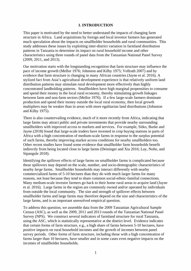
1. INTRODUCTION

This paper is motivated by the need to better understand the impacts of changing farm structure in Africa. Land acquisitions by foreign and local investor farmers has generated much speculation about the impacts on smallholder households and rural communities. This study addresses these issues by exploiting inter-district variation in farmland distribution patterns in Tanzania to determine its impact on rural household income and other characteristics using three rounds of panel data from the Tanzanian National Panel Survey (2009, 2011, and 2013).

Our motivation starts with the longstanding recognition that farm structure may influence the pace of income growth (Mellor 1976; Johnston and Kilby 1975; Vollrath 2007) and by evidence that farm structure is changing in many African countries (Jayne et al. 2016). A stylized fact from Asia’s agricultural development experience is that relatively uniform land distribution patterns may stimulate rural development more effectively than highly concentrated landholding patterns. Smallholders have high marginal propensities to consume and spend their money in the local rural economy, thereby stimulating growth linkages between farm and non-farm sectors (Mellor 1976). If a few large-scale farmers dominate production and spend their money outside the local rural economy, then local growth multipliers may be weaker than in areas with more egalitarian land distributions (Johnston and Kilby 1975).

There is also countervailing evidence, much of it more recently from Africa, indicating that large farms may attract public and private investments that provide nearby surrounding smallholders with improved access to markets and services. For example, Sitko, Burke and Jayne (2018) found that large-scale traders have invested in crop buying stations in parts of Africa with a high concentration of medium-scale farms in response to the surplus potential of such farms, thereby improving market access conditions for nearby smallholders too. Other recent studies have found some evidence that smallholder farm households benefit indirectly from being located close to large farms (Deininger and Xia 2016; Lay, Nolte, and Sipangule 2018).

Identifying the spillover effects of large farms on smallholder farms is complicated because these spillovers may depend on the scale, number, and socio-demographic characteristics of nearby large farms. Smallholder households may interact differently with nearby commercialized farms of 5-10 hectares than they do with much larger farms for many reasons, not least because they tend to share common social-ethnic-familial connections. Many medium-scale investor farmers go back to their home rural areas to acquire land (Jayne et al. 2016). Large farms in the region are commonly owned and/or operated by individuals from outside the local community. The size and strength of spillover effects between smallholder farms and large farms may therefore depend on the size and characteristics of the large farms, and is an important unresolved empirical question.

To address this question, we assemble data from the 2009 Tanzanian Agricultural Sample Census (ASC), as well as the 2009, 2011 and 2013 rounds of the Tanzanian National Panel Survey (NPS). We construct several indicators of farmland structure for rural Tanzania, using the ASC, which is statistically representative at the district level. Evidence indicates that certain forms of farm structure, e.g., a high share of farms between 5-10 hectares, have positive impacts on rural household incomes and the growth of incomes between panel survey periods. Other forms of farm structure, including those with a high concentration of farms larger than 10 hectares, have smaller and in some cases even negative impacts on the incomes of smallholder households.

2

Our primary question—whether or not the local structure of land ownership matters for rural growth—is important for several reasons. First, changes in farm structure are occurring rapidly in many Sub-Saharan African countries, with a major trend being one of increasing land concentration driven by medium- and large-scale land acquisitions in customary tenure systems (Jayne et al. 2014 2016; Sitko and Chamberlin 2016; Anseeuw et al. 2016). These studies suggest a de facto move towards greater land concentration. However, land concentration may be occurring in different ways. The contribution of our study is to emphasize the multi-dimensional nature of farm structure and land concentration, to demonstrate that alternative indicators of land concentration that emphasize different dimensions are often poorly correlated with one another, and most importantly to show how these alternative indicators of farm structure exert varying and in some cases very strong influences on the farm and non-farm incomes of rural households in the vicinity. The study concludes that if land distribution patterns matter for rural transformation, as is strongly indicated by our findings, then researchers and policy makers may need to more accurately understand how farm structure is changing under alternative land tenure systems and more explicitly consider the impact of farm structure on development outcomes and policy objectives.

The remainder of the paper is structured as follows: Section 2 expands on the theoretical relationships between farm structure and economic development outcomes in agrarian areas. Section 3 describes the data used in this study, and Section 4 discusses the challenges of empirically addressing our research question. Descriptive and econometric results are presented in Sections 5 and 6, respectively, followed by conclusions in Section 7.

3

2. CONCEPTUAL FRAMEWORK

2.1. Core Theoretical Perspectives

There are two competing ways in which we might think about the relationship between farm structure household income growth. The first of these is rooted in the seminal work of Johnston and Kilby (1975) and Mellor (1976), who emphasized the importance of growth multipliers as drivers of rural development. The core idea is that because the propensity to spend additional income on local goods and services is greatest for smallholder households, then virtuous cycles are engendered by broad-based agricultural growth in which income gains by smallholders are cycled through local farm and non-farm economies. Broad-based agricultural growth tends to generate greater second-round expenditures in support of local non-tradable goods and services in rural areas and towns. If, however, agricultural productivity and household income gains are concentrated within relatively few households (as might be the case in areas where a few large farms have a disproportionate share of land and production), then growth multipliers from agricultural surplus may be more limited, as compared with more egalitarian land distributions. Empirical work by Deininger and Squire (1998) and Vollrath (2007) support this idea, providing evidence that relatively egalitarian national-level land distribution patterns are associated with more broadly based agricultural productivity growth, and higher rates of growth, than more concentrated land distributions.

Other ways of thinking about the influence of land concentration on smallholder welfare posit different channels, but which are consistent with the above framework. For example, Berry and Cline (1979), using national-level data, found that the relative underutilization of agricultural land increases with the degree of inequality in land distribution. Sitko and Jayne (2014) describe similar findings for farm-level data from Zambia: larger farms had lower shares of land being used for cropping or other intensive productive activities than smaller holdings. Due to ethnic and social differences, large-scale and small-scale farmers may have little social interaction, minimizing potential synergies from learning, cooperation, and economic exchange, which could be important avenues by which productivity and income gains and spillovers may be realized

Also at the country-level, Binswanger and Deininger (1997), Engerman and Sokoloff (1997), and Sokoloff and Engerman (2000) discuss ways in which land inequality may be associated with institutional control. In particular, land concentration (inequality) is often associated with an elite class of rural landholders that wields political power; this power often limits the ability of non-elites to participate in political systems or benefit from public institutions such as crop marketing boards, input promotion programs, and education, which may condition household income. These processes may play out at both national, regional and local levels. For example, if large farms dominate in a particular area, they may influence the nature of local supply chains, such that input providers, commodity traders and other service providers are more oriented towards supporting larger farms in ways that are less accessible to smaller producers.

A countervailing hypothesis is that large farms (at least under some conditions) may generate important spillover benefits for smallholders operating in their vicinity. The surplus production of relatively large farms may attract private investment in crop buying, storage, transport, input supply and finance into rural areas, providing spillover benefits to all households in the areas (Collier and Dercon 2014). The political clout of large farmers may also attract state investment in infrastructure development, which would also benefit all farms in an area (von Braun and Meinzen-Dick 2009; Deininger and Xia 2016). Introduction of new production technologies may facilitate technological spillovers via knowledge transfers and increased access to agricultural technologies

4

(Kleemann et al. 2013; Rakotoarisoa 2011).1 Direct linkages between large and small farmers may also exist, e.g., out-grower schemes, contract farming arrangements, and the generation of wage employment opportunities. Where such arrangements are in place, knowledge transfer may be particularly strong (De Schutter 2011; Munjenja and Wonani 2012). To the extent to which such positive spillovers exist, then land concentration may promote income growth across all households in a shared location.

As it stands, the evidence base for either positive or negative impacts of large farm spillovers on nearby smallholders remains weak. Lay, Nolte, and Sipangule (2018) find some evidence for localized positive productivity spillovers of large agricultural investments to nearby smallholders in Zambia.2 Deininger and Xia (2016) find that large-scale investments produce short-run positive and negative effects on nearby smallholder farms in Mozambique. These studies identify the effects of spillover effects through a smallholder household’s physical proximity to the number of large-scale farms within a certain radius or whether there are any large farms within the locality. While this may be a reasonable approach for addressing specific kinds of questions, we believe that the effects of land concentration and spillover effects from particular kinds of farms may be more comprehensively understood by constructing measures that represent the full range of large, medium, and small farms within in a given area, as reflected in various measures of farm size distributions.3

Our main premise should now be clear, i.e., that different aspects of farm structure cannot be fully captured in one indicator such as the Gini coefficient, or the number of farms of a certain size in a given area. Conceptually, the pathways by which large farms may influence the behavior and welfare of nearby smallholder households may only incidentally be related to standard land inequality measures. Because farm structure is a multidimensional concept, empirical analysis seeking to understand the effects of alternative land distribution patterns on local growth patterns must consider alternative dimensions of farm structure.

2.2. Model of Per-Full Time Equivalent Gross Income Determinants

We may generalize the above ideas as follows. Let us start with a farm-level production function:

(1) 𝑌𝑌𝑖𝑖,𝑗𝑗,𝑡𝑡 = 𝜷𝜷𝜷𝜷𝑖𝑖,𝑗𝑗,𝑡𝑡 + 𝜸𝜸𝑪𝑪𝒋𝒋 + 𝜃𝜃𝜃𝜃𝑗𝑗,𝑡𝑡−1 + 𝝐𝝐𝑖𝑖,𝑗𝑗,𝑡𝑡

where Y is gross income per full-time equivalent (FTE) for farmer i in community j at time t; X is a vector of household-level characteristics, C is a vector of local geographic context characteristics, G is a measure of access to local public and private capital stocks in community j, and ε is an idiosyncratic error term. If we accept that (unobservable) access to local public and private capital stocks is conditioned by the (observable) localized distribution of land control, i.e.,

1 Such knowledge transfers from large to small farmers may take place directly, e.g., via technical assistance, formal and informal training and/or service provision, or indirectly, e.g., via learning-by-doing. 2 Empirical evidence is somewhat limited. Some literature uses firm level data (Javorcik 2004; Görg and Greenaway 2004), and does not focus on agriculture. At least two studies have provided evidence in support of large-scale land-based investments contributing to infrastructural improvements in the investment locations (Mujenja and Wonani 2012; FAO 2012). 3 In addition to the several studies cited here, we also found a few studies examining the impacts of large-scale farm investments on local communities using qualitative case study approaches (e.g., Cotula et al. 2009; Anseeuw et al. 2012).

5

(2) 𝜃𝜃𝑗𝑗,𝑡𝑡 = 𝑓𝑓(𝐼𝐼𝑗𝑗,𝑡𝑡 ,𝑍𝑍𝑗𝑗,𝑡𝑡)

where I is a measure of farmland structure in community j at time t, and Z is a vector of other factors which influence G, then we may rewrite an estimable production function as:

(3) 𝑌𝑌𝑖𝑖,𝑗𝑗,𝑡𝑡 = 𝜷𝜷𝜷𝜷𝑖𝑖,𝑗𝑗,𝑡𝑡 + 𝜸𝜸𝑪𝑪𝒋𝒋 + 𝛿𝛿𝐼𝐼𝑗𝑗,𝑡𝑡−1 + 𝛾𝛾𝑍𝑍𝑗𝑗,𝑡𝑡−1 + 𝝐𝝐𝑖𝑖,𝑗𝑗,𝑡𝑡

where δ is an estimable coefficient on observable farm structure. If δ<0, then the net effect of more concentrated land distribution patterns or the share of farmland controlled by medium or large farms on smallholder household incomes is negative. If δ>0, then positive spillovers dominate the relationship.

6

3. DATA AND VARIABLE CONSTRUCTION

3.1. Data Sources

Data used in this analysis come from two main sources. Data on household per-FTE gross income measures, along with other household- and community-level controls, were constructed from the Tanzanian National Panel Survey (NPS), available for three waves (2009, 2011, and 2013).4 Given the nature of our research question, we are interested in estimating impacts on households in rural areas. However, the census definitions of urban Standard Enumeration Areas (SEAs) in this sample are not urban in the conventional sense of being primarily composed of town dwellers without agricultural land and farming activities. Therefor we include households in urban SEAs which have relatively low population densities. (As a robustness check, we compare results with models estimated on samples which only include rural SEAs.) After dropping households which only appear in a single wave, we have an unbalanced panel of 8,540 observations across the three waves.

While the NPS is considered to be statistically representative of households in rural Tanzania, it may not have sufficient observations to be statistically representative of the full range of farm sizes found in Tanzania (Christiaensen and Demery 2018). We therefore constructed indicators of farm structure from the Tanzanian Agricultural Sample Census (ASC) for 2009. The ASC contains data on 52,635 rural agricultural households randomly selected from the prior census, as well as all 1,006 farms categorized as large scale5 that were identified in the country at the time. The ASC enables district-level inference, but the large-farm component only contains regional identifiers. We thus faced a quandary: either construct measures of farm structure at the more localized district level (n=142) and omit the large farm module, or construct measures of farm structure at the much larger region level (n=26) that include the large farm module. To make this decision, we constructed the Gini coefficient and other measures of farm structure at the region level, first including the large farm module and then excluding it. As will be shown below, these measures are highly correlated and the rank order of inequality among districts is virtually the same regardless of whether the large-farm module is included or not. From this we conclude that the district-level indicators are not sensitive to omitting the large farm component. And because the district-level indicators enable us to examine the relationship between farm structure/inequality and household incomes at a more disaggregated geographic level, we proceeded to carry out the analysis in this way.

3.2. Variable Construction

Household landholdings are defined in this analysis as all the land controlled by the household, including land that is cultivated, in fallow, undeveloped, under pasture, planted with trees or other permanent crops, or any other land usage. For every household in the sample, the total landholding size is constructed as the sum of plot-level records.

4 The Tanzanian NPS is part of the LSMS-ISA program supported by the World Bank. 5 Large scale farms were defined on the basis of landholdings (>20 hectares) as well as a number of other criteria, which allowed some smaller holdings to be included (e.g. operating at least 0.5 ha of intensive greenhouse horticultural production). See National Bureau of Statistics (2012: p11) for more details.

7

3.1.1. Variables Measuring Farm Structure and Land Concentration

Our exogenous variables of main interest pertain to farm structure and land concentration. There are many alternative possible measures, including (i) the Gini coefficient; (ii) skewness (third standard moment); (iii) coefficient of variation (standard deviation/mean); (iv) share of operated farmland on farms between 5 to 10 hectares; and (v) share of operated farmland on farms over 10 hectares. Each of these variables measure different aspects of farm structure, with some emphasizing the importance of specific scales of farm operation, while others focus more on the degree of concentration of landholdings. Because of this, we do not necessarily expect these indicators to be highly correlated.

Figure 1 shows stylized landscapes which represent alternative farm size configurations of a constant total area. Concentration metrics are calculated for each, and shown in the figure. For the most part, these correspond with an intuitive understanding of concentration in that, as we progress from the upper left, through the upper right, lower left and lower right, we have generally increasing values in most metrics.

Figure 1. Stylized Landscapes and Corresponding Land Concentration Measures

Landscape 1:Total ha = 58# farms = 27

Concentration:Gini = 0.064Skewness = 3.253CV = 0.248%ha>10ha = 0.000

Landscape 3:Total ha = 58# farms = 9

Concentration:Gini = 0.544Skewness = 2.132CV = 1.429%ha>10ha = 0.517

Landscape 2:Total ha = 58# farms = 12

Concentration:Gini = 0.302Skewness = 0.173CV = 0.597%ha>10ha = 0.000

Landscape 4:Total ha = 58# farms = 5

Concentration:Gini = 0.662Skewness = 1.500CV = 1.851%ha>10ha = 0.862

= 2 ha

50 ha

30 ha

8 ha4 ha

8

3.1.2. Outcome Variables

Our key outcome variables of interest are per-FTE (full-time equivalent) income measures. These are constructed using household-level earnings divided by the household sum of individual-level full-time equivalent values calculated from labor-allocation data as recorded by the NPS. Four main categories of income are considered: farm, non-farm, agricultural wages, and total income. Farm income includes income from crop production and livestock income (which, in turn, comprises value of sales of live animals, value of slaughtered animals, and value of production of milk, eggs, honey, hides, and skins). Non-farm income includes income from non-farm business activities and off-farm wage employment (including agricultural wage labor). Agricultural wage employment income was also included as a separate category. Finally, total income is the sum of farm, agricultural wage, and non-farm income.

3.1.3. Full-time Equivalents

To calculate FTEs, we add up the hours an individual household member reports allocating to on-farm activities, non-farm business activities, and wage employment activities. For any given individual, the total hours per week spent working cannot exceed 112 (=16 hours * 7 days). If the amount reported across all categories exceeds this amount, we scale hours in each category proportionally, such that 112 hours per week is not exceeded. All monetary values were converted to real 2010 USD.

9

4. IMPLEMENTATION CHALLENGES

There are several important challenges in estimating our model of interest. These include data quality constraints, an inherent arbitrariness in defining measures of land concentration, and endogeneity issues in ascertaining impacts of land concentration on growth outcomes.

4.1. Data Quality Issues

The Tanzanian National Panel Surveys, described above, are limited in how information on per-FTE gross income was collected. First of all, for wage income, the amount worked by an individual over the previous 12 months was only calculated for the last two waves. Furthermore, while the second and third waves asked about primary and secondary jobs, the first wave only asked about the primary job. Thus, we were not able to use the first wave of the NPS (2008) in this analysis.

Even though total time worked for wage income over the previous year was nominally recorded (via three questions: “During the last 12 months, for how many months did you work in this job?”, “During the last 12 months, how many weeks per month do you usually work in this job?” and “During the last 12 months, how many hours per week do you usually work in this job?”), the informal nature of much wage employment in Tanzania (perhaps particularly in rural areas) implies a high degree of variability, which may not easily filter through such averaging questions. The upshot of this is that our income data are somewhat noisy, as are our measures of per-FTE gross income based thereon. Measurement error in the dependent variable does not bias coefficient estimates but it may inflate their standard errors (Wooldridge 2010). To address sensitivity of estimation results to such noise, we also estimate regression models for dependent variables which are not normalized by FTEs (i.e., on household-level income measures). These regression results differ little from our per-FTE measures, and we therefore report results from the per-FTE models.

4.2. Endogeneity Concerns

In estimating our model of interest, equation (3), there are several endogeneity concerns. The first of these is that localized farm structure and per-FTE gross income may be jointly driven by unobserved factors. For example, if land concentration is associated with commercial land investments that target areas of favorable agro-ecological or market access conditions, we may get upwardly biased coefficient estimates. We take four steps to control for this. First, we include available agro-ecological and market access controls in our regression models (described in detail below). Second, we include year, region, and year*region dummy variables to control for unobserved time-constant and time-varying regional effects. Third, to reduce the possibility of simultaneity, our land concentration measures are constructed from the first survey in 2009, while our household-level income measures and other controls are defined for 2011 and 2013.

While the first and second steps above can control for unobserved regional effects, there remains the issue of unobserved heterogeneity at the household level. To address this, our fourth step is to exploit the panel nature of the data to incorporate the Mundlak-Chamberlain (MC) device (Mundlak 1978; Chamberlain 1984) into our models, giving us an estimator that Wooldridge (2010) refers to as the Correlated Random Effects model. The MC device employs household-level averages of all time-varying components of the model in order to control for unobserved time-constant heterogeneity, under the assumption that such

10

heterogeneity is correlated with the time-averages. While we cannot fully eliminate all potential sources of endogeneity, we feel that the four steps described here go as far as possible to do so with the available data.

4.3. Attrition

A third concern is potential attrition bias arising from the use of panel data. We test for this and fail to reject the null hypothesis of no attrition bias in our models. We therefore define and implement attrition weights in all of the regression models, following the methods described in Baulch and Quisumbing (2011).6

6 In practical terms, we find that whether or not we use attrition weights, our coefficient estimates change very little, and the overall analytical conclusions are the same. Nonetheless, because we do not reject the null hypothesis of zero attrition bias, we report results from the weighted models in this paper. Unweighted model results are also available from the authors upon request.

11

5. DESCRIPTIVE RESULTS

5.1. Farm Size Structure

The Tanzanian farm sector is dominated by smallholdings, as elsewhere in the region. However, measures of farm structure are sensitive to choice of dataset. Table 1 shows distributions of farm sizes across the country, using the NPS and ASC for 2009. Three observations are highlighted here. First, the distribution of farm holdings using NPS is sensitive to whether landless households are included in the analysis, at least at very low percentiles of the distribution. Less than 1% of rural Tanzanian households are found to be landless. Second, and more importantly for our analysis, farm sizes start to diverge between NPS and ASC at high ends of the farm size distribution. At the 95th percentile, the ASC shows farm size to be 8.1 hectares compared to 6.8 hectares for NPS. At the 99th percentile, the ASC shows farm size to be 33.8 or 31.7% higher than that of NPS, depending on whether the ASC’s large-scale module is included or not. Third, the distribution of farm sizes for ASC up to the 99th percentile is virtually the same regardless of whether the large-scale farm module is included or not. As mentioned earlier, we can define district-level measures of farm structure using ASC only if the large-scale module is excluded, which fortunately has little bearing on most indicators of farm structure. Given the much larger sample size of the ASC and its statistical representativeness at district level, we prefer it to the NPS for constructing indicators of farm structure and land concentration.

5.2. Income Trends, by Farm Size Category

Table 2 below shows changes over time in per-FTE income measures for three farm size categories using the balanced panel of NPS households between 2009 and 2013. We had to define farms over five hectares as the largest category because NPS contains few farms over 10 hectares. Overall, household incomes per FTE rose by 7% in real terms between 2009 and 2013.

Table 1. Farm Structure in Tanzania

Hectares per farm holding at the xth percentile

of weighted sample distribution

5th 10th 25th 50th 75th 90th 95th 99th mean

Controlled land (NPS) 0.1 0.3 0.6 1.3 2.4 4.5 6.7 14.6 2.3

Controlled land (NPS) – excluding landless HHs 0.3 0.4 0.8 1.4 2.6 4.5 6.8 15.1 2.4

Controlled land (ASC: large-scale module included

0.4 0.4 0.8 1.6 2.8 4.9 8.1 20.2 2.7

Controlled land (ASC: large-scale module excluded

0.4 0.4 0.8 1.6 2.8 4.9 8.1 19.8 2.5

Note: NPS data for 2008/2009; ASC data for 2009. NPS households in sampling areas designated as urban are excluded from the calculation.

12

Table 2. Measures of Household Income per FTE, by Farm Size Category

Landholding size category

2009 2011

2013 Avg.

annual growth

sample size in 2013 Values in 1000s of

real 2013 TSh

Agricultural income per-FTE

<2 ha 119 104 115 -1% 1,673 2-5 ha 202 187 233 4% 688 > 5 ha 290 336 320 3% 347

Non-farm income per-FTE

<2 ha 423 514 594 10% 1,673 2-5 ha 443 461 526 5% 688 > 5 ha 426 413 578 9% 347

Agricultural wage income per-FTE

<2 ha 92 113 123 8% 1,673 2-5 ha 82 105 137 17% 688 > 5 ha 43 118 78 20% 347

Total per-FTE gross income

<2 ha 554 639 719 7% 1,673 2-5 ha 682 694 881 7% 688 > 5 ha 784 838 1,077 9% 347

Source: NPS. Landholding size categories are based on the controlled area, which includes all plots which are reported as cultivated, fallow, virgin, forest and pasture. The sample is restricted to rural areas and households with at least one reported plot. The top 1% of income values are dropped as outliers. Zero-valued income is included. Agriculture incomes per FTE were stagnant over this period. Non-farm and agricultural wage incomes were the main source of income growth during this period, rising by 8% and 12%, respectively.

Disaggregation by farm size category shows that total household income per FTE growth over the 2009-2013 period was remarkably similar over the distribution of farm size categories. Household agricultural incomes grew faster for farms over 5 hectares than for the majority of farms below 2 hectares. In contrast, households with small farms experienced more rapid non-farm income growth. This is consistent with other analyses showing a shift in Tanzania’s employment patterns from farm to off-farm and non-farm sources of income in recent years (Yeboah and Jayne 2018).

5.3. Land Concentration Measures

To evaluate sensitivity of land concentration indicators to choice of landholding dataset, we constructed land concentration measures at the national level from both the NPS and ASC for 2009 (Table 3 below). Comparing measures constructed using the small farm component of the ASC with measures from the NPS, we find that measures differ substantially from one another in some respects and very little in other respects. As expected, when including the large scale farm component of the ASC, some measures are substantially higher, e.g., skewness, coefficient of variation (CV) and the share of land under farms of 10 or more hectares, although other measures are very similar with those based on only the small farm portion (Gini and the share of land in farms of 5-10 hectares).

13

Table 3. National Measures of Farm Structure from Alternative Data Sources Dataset

Measure of land concentration NPS

NPS (landless excluded)

ASC (excl. large farm module

ASC (incl. large farm module)

Gini 0.58 0.56 0.53 0.57

Skewness 25.5 25.1 15.8 512.8

Coefficient of variation 3.19 3.12 1.77 17.95

Share of land held by farms 5-10 ha 0.17 0.17 0.16 0.15

Share of land held by farms > 10 ha 0.24 0.24 0.23 0.38

Note: NPS data for 2008/2009; ASC data for 2009. Land measures calculated on controlled land (including rented land). Landless households are included in the calculations, except in column 2. To be consistent with ASC, NPS households in sampling areas designated as urban are excluded from the calculation.

Table 4. Correlation Matrix of Farm Structure Measures, District Level

Gini Skewness CV

% land under farms of 5-10ha

Gini 1

Skewness 0.4171 *** 1

CV 0.7119 *** 0.8162 *** 1

% land in farms 5-10 ha 0.3567 *** 0.0728 0.1279 1

% land in farms > 10 ha 0.7331 *** 0.3725 *** 0.5576 *** 0.5407 ***

Source: ASC data for 2009. Landholding based on land controlled (i.e., includes non-cultivated plots). *** denotes significance at the 1% level.

To further explore the comparability of alternative farm structure measures, we construct correlation matrices for alternative indicators at the region level (Table 4). Alternative indicators correlate imperfectly with one another. This should not be considered surprising considering that they emphasize different aspects of farm structure. In any case, the results in Tables 3 and 4 point to the need to evaluate the robustness of our results to the choice of alternative farm structure indicators.

Given the possible distortion of district-level land concentration measures from the ASC which are not able to include the large farm component, we evaluate the correlation of measures constructed at the regional level (which does permit inclusion of the large-farm module). Comparing such region-level measures constructed with and without the large farm sample, we find that most regions do not vary much. As an example, comparisons of Gini coefficients are shown in Figure 2. Nonetheless, to account for potential biases in our regression work relying on district-level concentration measures, we include a dummy variable to identify regions where the inclusion of the large farm component results in

14

differences in Gini coefficient calculations by 10% or more. As can be seen in the appendix table results, these dummies where generally statistically insignificant, signifying no unique impacts of these districts compared to the others.

Figure 2. Scatterplot of Gini Coefficients on Landholdings from Agricultural Sample Census with and without Large Farm Sample, Region Level

Source: Tanzanian National Bureau of Statistics 2009.

R² = 0.7335

0.3

0.4

0.5

0.6

0.7

0.3 0.35 0.4 0.45 0.5 0.55 0.6 0.65 0.7

Regi

onal

Gin

i fro

m A

SC (s

mal

l onl

y)

Regional Gini from ASC (sm+lg)

Regional Gini coefficients on landholding size

15

6. ECONOMETRIC ANALYSIS

6.1. Baseline Specification

Coefficient estimates for land concentration measures from our baseline regression specifications are shown in Table 5 (the full set of results are shown in Appendix Table A1). There are 4 dependent variables: (a) agricultural per-FTE gross income, (b) non-agricultural per-FTE gross income, (c) off-farm agricultural per-FTE gross income, and (d) total per-FTE gross income. All of these dependent variables are transformed using the inverse hyperbolic sine transformation (MacKinnon & Magee 1990). Because most of this function’s domain approximates that of a logarithm, the coefficient estimates can be interpreted as one would in a log-level specification. For each of these dependent variables, the specifications differ only in the choice of farm structure measure: (i) Gini coefficient, (ii) skewness, (iii) coefficient of variation, (iv) share of land in farms of 5-10 hectares, (v) share of land in farms of >10 hectares, and (vi) share of land under farms of 5-10 and >10 hectares, respectively. Because initial testing indicated that panel attrition was influenced by variables in our models, these specifications all use inverse probability weights to correct for the probability of household attrition. However, it is noted that weighted and unweighted regressions differ very little in the resulting coefficient estimates.

The main analytical conclusion is as follows: while impacts on any particular income type are highly dependent upon which farm structure is used, the overall impacts of more concentrated landholding patterns on farm, non-farm and total per-FTE gross income is generally positive and statistically significant. The impact of the share of land in medium-scale farms (between 5 and 10 hectares) is particularly pronounced and highly significant. The higher the share of district farmland among farms 5 to 10 hectares, the greater the impact on farm, non-farm and total incomes among households within the district. This positive contribution of medium-scale farms does not appear to carry over to farms larger than 10 hectares. In fact, a higher share of district farmland under farms over 10 hectares has negative and significant influences in the non-farm and agricultural wage models. This suggests that commercial operations over 10 hectares in our sample may not engender the same kinds of positive spillover effects as with medium-scale farms of 5-10 hectares.7 This finding is consistent with the idea that income multipliers are smaller when very large farms possess a relatively large portion of the land under production in a localized farm-based economy.

Given the predominance of gendered differences in land access in Sub-Saharan Africa (Doss et al. 2013), we considered the possibility that land concentration may be correlated with poorer access to land by women (in which case gendered land access would constitute an omitted variable that is correlated with and biasing the coefficient on land concentration. To address this concern, we first note that in all specifications (including all the baseline specifications shown in the Appendix), the female-head dummy is not significant. Furthermore, when we specify a model which interacts the female-head dummy with the land concentration measures, the coefficient estimate for the interaction term is not significantly different from that of the non-interacted term. This provides some reassurance that a gendered access story is not driving our results.

7 For reference, mean and median farm sizes of farms greater than 10 hectares in the ASC sample are 15 and 25, respectively (14 and 19, when not including the commercial farm component). As a robustness check on these findings, we also ran models with alternative definitions of land concentration, e.g. share of land in 5-20 ha farms, 20+ ha farms, etc. For all of the alternative definitions we checked, the same basic results were obtained, i.e., the coefficient on share of land in the medium-scale category was significant and positive, but decreasing in magnitude with the width of the category (i.e., the positive impact of the coefficient on the share of land under 5-10 ha farms is smaller in magnitude than the coefficient on the share of land under 10-20 ha farms); the coefficient on share of land in the largest category (whether >10, >20 or >50 ha) was invariably insignificant.

16

Table 5a. Selected Coefficients from Baseline Regression Models: Household Farm per-FTE Gross Income (1) (2) (3) (4) (5) (6) Land Concentration Gini 2.620*** (4.64e-05) Skewness 0.0248* (0.0862) CV 0.295*** (0.00657) Share land: farms 5-10 ha 1.951*** 1.809*** (0.00147) (0.00683) Share land: farms >10 ha 0.466 0.143 (0.113) (0.656)

Table 5b. Selected Coefficients from Baseline Regression Models: Household non-Farm per-FTE Gross Income (1) (2) (3) (4) (5) (6) Land Concentration Gini 1.297 (0.288) Skewness 0.0214 (0.498) CV 0.147 (0.470) Share land: farms 5-10 ha 4.393*** 5.827*** (0.00109) (7.56e-05) Share land: farms >10 ha -0.416 -1.467** (0.503) (0.0308)

17

Table 5c. Selected Coefficients from Baseline Regression Models: Household Agricultural Wage per-FTE Gross Income (1) (2) (3) (4) (5) (6) Land Concentration Gini -0.959 (0.390) Skewness -0.0208 (0.485) CV -0.177 (0.360) Share land: farms 5-10 ha 1.696 2.858** (0.181) (0.0414) Share land: farms >10 ha -0.670 -1.188* (0.249) (0.0645)

Table 5d. Selected Coefficients from Baseline Regression Models: Total Household per-FTE Gross Income (1) (2) (3) (4) (5) (6) Land Concentration Gini 1.910*** (1.73e-05) Skewness 0.0133 (0.266) CV 0.222*** (0.00528) Share land: farms 5-10 ha 1.666*** 1.658*** (0.000971) (0.00257) Share land: farms >10 ha 0.306 0.00803 (0.177) (0.974)

Notes: Dependent variables are inverse hyperbolic sine transformed per-FTE gross income measured in 2010 constant Tanzanian shillings. District-level land concentration measures from 2009 Ag. Sample Census. Dependent variables and other independent control variables are from the NPS. All models include the Mundlak- Chamberlain device. Full model results shown in Appendix A1. Robust pval in parentheses, with significance indicated by asterisks: *** p<0.01, ** p<0.05, * p<0.1.

18

To test the robustness of these findings, we estimated a large number of alternative specifications. To begin with, to allay concerns about potentially noisy per-FTE income measures, we also estimate models using farm-level income measures (i.e., not normalized by household FTEs for any given income category) as dependent variables. Coefficient estimates from these models are extremely similar to the per-FTE measures. We also estimated models using a sample restricted to households in enumeration areas defined as rural by the Tanzanian National Bureau of Statistics, to address the possibility that our results are influenced by households which are not truly rural; results are very similar in this case as well. To address concerns about omission of the large farm component of the ASC in our district-level land concentration measures, we estimated models using regional-level concentration measures which include the large-farm component. In all case, estimation results differ very little in substantive terms.

6.2. Interacting Concentration with Household Asset Dummies

Table 6 shows results from model specifications which interact regional land concentration measures with household-specific productive asset categories, defined as terciles of the sample distribution. For conciseness, we only show model results where the dependent variable is agricultural per-FTE income. Full estimation results are shown in Appendix A2. While impact estimates vary across land concentration measures and their interactions, a general pattern may be observed in which the positive impacts of land concentration are larger for the top two asset terciles. Relatively poor households benefit the least from localized land concentration (and in some cases are significantly worse off from it), whereas the majority of households and especially the wealthiest one-third of households tend to benefit significantly.

These differential wealth-related impacts on farm income indicate that spillover effects from land concentration are not equally accessible to all farms within an area. Even though Sitko, Burke and Jayne (2018) found that medium-scale farms tend to attract private traders and improve market access conditions for nearby smallholders, relatively poor households may not be able to benefit from this if they cannot produce a farm surplus in the first place. While van der Westhuizen et al. (2018) found that medium-scale farmers tend to rent out their tractors to small-scale farms in their areas, relatively poor households may not be able to afford to take advantage of such services. While we feel these interpretations are quite plausible in light of other evidence, our data do not allow us to do more than surmise what specific channels of spillover may be taking place. These results are very similar to results of models (not shown here) that use farm size categories in place of household asset categories, which is not surprising given the high correlation between asset wealth and land holding size.

19

Table 6. Selected Coefficients from Regression Models of Household Farm Income per-FTE Including Interaction Terms between Land Concentration and Asset Terciles Dep. var: farm per-FTE gross income (1) (2) (3) (4) (5)

Land concentration Gini 0.941 (0.299) Gini * medium 1.841*** (0.00526) Gini * wealthiest 2.306*** (0.00148) Skewness -0.0780* (0.0766) Skewness * medium 0.111** (0.0144) Skewness * wealthiest 0.124*** (0.00789) CV -0.0801 (0.690) * medium 0.421** (0.0344) * wealthiest 0.506** (0.0183) share land: farms 5-10 ha -2.948* (0.0991) * medium 4.876*** (0.00602) * wealthiest 5.749*** (0.00172) share land: farms >10 ha -0.514 (0.387) * medium 1.611** (0.0183) * wealthiest 1.119* (0.0756)

Notes: Dependent variables are inverse hyperbolic sine transformed per-FTE gross income measured in 2010 Tanzanian shillings. District-level land concentration measures from 2009 Ag. Sample Census. Dependent variables and other independent control variables are from the NPS. All models include the Mundlak-Chamberlain device. Full model results shown in Appendix A2. Robust pval in parentheses, with significance indicated by asterisks: *** p<0.01, ** p<0.05, * p<0.1. 6.3. Inter-Period Income Changes Regressed on Lagged Independent Variables

As an alternative specification of our basic model, we regressed the changes in household income (measured as the average annual growth in the two-year period between panel waves) against lagged exogenous regressors in the following form:8

8 Although this equation expresses a log-linear relationship, the dependent variable we use in the models we report on in this paper is transformed with the inverse hyperbolic sine transform. Because these transformations

20

(4) ∆𝑙𝑙𝑙𝑙𝑙𝑙𝑌𝑌𝑖𝑖,𝑗𝑗,(𝑡𝑡,𝑡𝑡−1) = 𝜷𝜷𝜷𝜷𝑖𝑖,𝑗𝑗,𝑡𝑡−1 + 𝛿𝛿𝐼𝐼𝑗𝑗,𝑡𝑡−1 + 𝛾𝛾𝑍𝑍𝑗𝑗,𝑡𝑡−1 + 𝝐𝝐𝑖𝑖,𝑗𝑗,(𝑡𝑡,𝑡𝑡−1)

Estimation results (shown in Appendix A3), while generally less precisely measured, are otherwise similar in the sign and magnitude of coefficient estimates as those of our baseline estimations. These results are consistent with the overall story coming from the other specifications shown in this section, i.e., a growth-promoting effect of more concentrated farm structure, but with less statistically significant effects.

6.4. Simulated Impacts of Changes in Density

To understand the magnitude of these impacts, we simulate the impacts of a change in the farm structure variables on total and farm per-FTE income, using the baseline results in Table 5. We consider a change in land concentration, moving from the 25th percentile to the 75th percentile. For example the 25th and 75th percentiles of the farmland Gini coefficient in our sample are 0.41 and 0.53, respectively).9 Results, shown in Table 7 below, indicate that such an increase in land concentration, as measured by the Gini coefficient, is associated with an average gain of 2 million TSh in total per-FTE gross income (about 1,380 USD), which is equivalent to more than doubling the mean level of total per-FTE gross income in our dataset. The estimated impact of increasing the share of land under medium-scale farms from the 25th to the 75th percentile is even larger.

While there is considerable variation in the impact estimates across alternative land concentration measures, the magnitude of these impacts indicate that the localized pattern of farm structure can exert a major influence on household incomes and livelihoods. We find these findings to be very plausible in light of growing evidence that medium-sized farms are attracting private investments in a variety of ways that are improving market access conditions for all rural residents in an area. Anecdotal evidence also suggests that medium-scale farms are a major source of cash expenditures in the local non-farm economy, potentially increasing the demand for a wide variety of goods and services locally (e.g., Poulton 2018).

are very similar in most of their domains (with the exception of very small values), we leave the log-linear notation in this equation for the sake of readability. 9 Here, we measure percentiles in terms of the sample-weighted households in our dataset, i.e., we compare the land concentration experienced by the sample household at the 25th percentile, when households are ranked by that land concentration measure, to that experienced by the household at the 75th percentile.

21

Table 7. Simulated Impacts of Changes in Land Concentration on Total Income and Farm Income (a) (b) (c) (d) (e)

Land concentration measure

Average per-FTE income predicted for land concentration at 25th percentile

Average per-FTE income predicted for land concentration at 75th percentile

difference (b) - (a)

difference as % of mean per-FTE income

difference as % of median per-FTE income

(1000s of 2010 TSh)

(1000s of 2010 TSh)

(1000s of 2010 TSh)

Farm per-FTE income:

Gini 444 744 300 57% 58% CV 804 851 46 9% 9% Share of land: 5-10 ha farms 1,206 1,730 524 99% 102%

Total income per-FTE income:

Gini 4,277 6,287 2,010 112% 106% CV 7,686 8,033 347 19% 18% Share of land: 5-10 ha farms 11,594 16,292 4,698 261% 247%

Note: Values in columns (a), (b) and (c) are thousands of real 2010 Tanzanian shillings (TSh). In 2010, 1 USD ≈ 1450 TSh. These simulation results based on the baseline regression specifications for farm- and total income, i.e., specifications corresponding to results shown in columns 1-4 and 13-16 in Tables 6 and A3.

22

7. CONCLUSIONS

This paper is motivated by the need to better understand the impacts of changing farm structure in Africa. Recent research has documented the rapid pace of new land acquisitions by foreign large-scale interests (Deininger and Byerlee 2011) and by medium-scale African farmers (Jayne et al., 2016). Tanzania in particular has experienced a rapid increase in land controlled by medium- and large-scale farms in recent years (Schoneveld 2014; Jayne et al. 2016). These changes in farm structure and composition have generated much speculation and debate about the impacts on smallholder households and rural communities, unfortunately with very little hard evidence to guide land policies and programs. Recent analysis has addressed the potential for spillover effects of large farms on technology adoption and yields of nearby smallholder farms, but the broader impacts on household incomes, disaggregated by farm and non-farm sources, and how these impacts may differ according to gender and wealth characteristics of the household have yet to be explored. Moreover, the few studies on this topic tend to identify the effects of large farms based only on proximity to a given smallholder household, without considering potential differences in impacts between large-scale and medium-scale farms or the degree of concentration of such farms within a given locality. This study addresses these issues by characterizing the structure of farm operations at the district level in Tanzania, both in terms of the relative importance of small, medium, and large farms, as well as by various indicators of farmland concentration in the locality. We then measure whether different kinds of farm structure are beneficial or detrimental to rural development as measured by rural household incomes, disaggregating the effects on income from own farming, agricultural wages, and non-farm sources. Farm structure indicators are derived from a unique Agricultural Sample Census carried out in Tanzania in 2009, which is statistically representative for the country’s 142 districts.10

Our first observation is that alternative indicators of farm structure chosen for this study differ considerably from one another. Some indicators emphasize the relative importance of different scales of farm operations in the locality, while others focus on the degree to which farmland operations are concentrated or unequally distributed. These observations reinforce a point that should already be well accepted—that farm or agrarian structure is a multifaceted concept and that specific indicators of agrarian structure may not be highly correlated with one another. For this reason, the impacts of different farm structures are likely to be highly sensitive to the choice of indicator.

Guided by these findings, we estimate several models of household income per full-time labor equivalent using panel estimation techniques, based on five alternative indicators of farm structure, including: (i) the Gini coefficient; (ii) skewness; (iii) coefficient of variation; (iv) share of controlled farmland under medium-scale farms; and (v) share of controlled farmland under large farms (defined as farms of 10 or more hectares).

The study highlights four main findings. First, farmland concentration is generally positively associated with rural household incomes, after controlling for other geographical and household-level factors. Second, household incomes from farm, agricultural wage and non-farm sources are particularly positively and significantly associated with the share of land in the district under farms of 5-10 hectares. Third, these positive spillover benefits are smaller and less statistically significant in districts with a relatively high share of farmland under farms over 10 hectares in size. While our econometric results do not identify the reason why medium-scale farms appear to generate greater spillover effects to local

10 The number of districts has since increased. As of the 2012 census, there were 169 districts in Tanzania.

23

communities than relatively large farms, recent published studies give us some clues – most medium-scale farmers come from the same social and ethnic backgrounds as small-scale farmers, and tend to have more extensive social interactions with the local community than do most large-scale farms (Sitko and Jayne 2014). Fourth, poor rural households are least able to capture the positive spillovers generated by medium-scale farms and by concentrated farmland patterns. The greatest benefits to household income were enjoyed by households in the upper two-thirds of the wealth distribution, which still includes the majority of rural households. We speculate that poor rural households are less able to afford taking advantage of the improved access to markets and services that medium-scale farms tend to provide. However, more detailed research is needed on the pathways by which medium- and large-scale farms affect household and broader local community welfare.

We believe that this paper contributes to our understanding of how various dimensions of farm structure may uniquely influence rural development trajectories, both conceptually and empirically in a particular African context. Moreover, our study underscores the importance of good data on land distribution in developing countries. The recent bounty of nationally representative data available through such initiatives as the World Bank’s LSMS-ISA program is certainly to be applauded. Nonetheless, we would advocate for even greater investments in expanding the sampling frame – both to ensure adequate representation of larger farms and to enable more spatially disaggregated measures of farm structure and concentration. Although this will require increased investments in data collection, the analytical payoffs stand to be substantial, particularly in countries where medium- and large-scale land acquisitions are known to be taking place. Much of the land acquisitions are occurring under the radar of traditional data collection mechanisms, and in some cases these land transfers may be transforming rural farm structure quite rapidly (Schoneveld 2014; Jayne et al. 2016). Ultimately, the scope for research to inform and guide African states will depend upon how well researchers and policymakers are able to accurately monitor and evaluate these changes taking place on the ground.

24

REFERENCES

Anseeuw, Ward, Mathieu Boche, Thomas Breu, Markus Giger, Jann Lay, Peter Messerli, and Kerstin Nolte. 2012. Transnational Land Deals for Agriculture in the Global South: Analytical Report Based on the Land Matrix Database. Bern/Montpellier/Hamburg: CDE/CIRAD/GIGA.

Anseeuw, Ward, T.S. Jayne, R. Kachule, and J. Kotsopoulos. 2016. The Quiet Rise of Medium-Scale Farms in Malawi. Land 5.3: 19. doi:10.3390/land5030019.

Baulch, Bob and Agnes Quisumbing. 2011. Testing and Adjusting for Attrition in Household Panel Data. CPRC Toolkit Note. Chronic Poverty Research Centre. Mimeo. Revised: 22 September 2011.

Berry, A.R. and W.R. Cline. 1979. Agrarian Structure and Productivity and Developing Countries. Baltimore: The Johns Hopkins University Press.

Binswanger, H.P. and K. Deininger. 1997. Explaining Agricultural and Agrarian Policies in Developing Countries. Journal of Economic Literature 35.4: 1958-2005.

Chamberlain, G. 1984. Panel Data. In Handbook of Econometrics, Volume 2, ed. Z. Grilliches and M.D. Intriligator. Amsterdam: North-Holland Press.

Christiaensen, L. and L. Demery (eds), 2018. Agriculture in Africa: Telling Myths from Facts. Directions in Development. Washington, DC: World Bank.

Collier, Paul and Stephan Dercon. 2014. African Agriculture in 50 Years: Smallholders in a Rapidly Changing World? World Development 63: 92-101.

Cotula, L., S. Vermeulen, R. Leonard, and J. Keeley. 2009. Land Grab or Development Opportunity? Agricultural Investment and International Land Deals in Africa. Rome; London: Food and Agriculture Organization of the UN (FAO); /International Fund for Agricultural Development (IFAD); and /International Institute for Environment and Development (IIED). Retrieved from http://www.iied.org/pubs/display.php?o=12561IIED.

De Schutter, O. 2011. How Not to Think of Land-Grabbing: Three Critiques of Large-Scale Investments in Farmland. The Journal of Peasant Studies 38.2: 249-279.

Deininger, K. and D. Byerlee, with J. Lindsay, A. Norton, H. Selod, and M. Stickler. 2011. Rising Global Interest in Farmland: Can It Yield Sustainable and Equitable Benefits? Washington, DC: The International Bank for Reconstruction and Development/The World Bank.

Deininger, K. and L. Squire. 1998. New Ways of Looking at Old Issues: Inequality and Growth. Journal of Development Economics 57.2: 259-87.

Deininger, K. and F. Xia. 2016. Quantifying Spillover Effects from Large Land-based Investment: The Case of Mozambique. World Development 87. November: 227-241.

Doss, Cheryl, Chiara Kovarik, Amber Peterman, Agnes R. Quisumbing, and Mara van den Bold. 2013. Gender Inequalities in Ownership and Control of Land in Africa: Myths versus Reality. IFPRI Discussion Paper No. 01308. Washington, DC: Poverty, Health, and Nutrition Division, International Food Policy Research Institute.

25

Engerman, S.L. and K.L. Sokoloff. 1997. Factor Endowments, Institutions and Differential Paths of Growth among New World Economies. In How Latin America Fell Behind, ed. S.H. Haber. Stanford CA: Stanford University Press.

FAO. 2012. Trends and Impacts of Foreign Investment in Developing Country Agriculture. Rome: FAO.

Görg, H. and D. Greenaway. 2004. Much Ado about Nothing? Do Domestic Firms Really Benefit from Foreign Direct Investment? The World Bank Research Observer 19.2: 171-197.

Javorcik, B.S. 2004. Does Foreign Direct Investment Increase the Productivity of Domestic Firms? In Search of Spillovers through Backward Linkages. The American Economic Review 94.3: 605-627.

Jayne, Thomas S., Jordan Chamberlin, Lulama Traub, Nicholas Sitko, Milu Muyanga, Felix K. Yeboah, Ward Anseeuw, Antony Chapoto, Ayala Wineman, Chewe Nkonde, and Richard Kachule. 2016. Africa’s Changing Farm Size Distribution Patterns: The Rise of Medium-Scale Farms. Agricultural Economics 47 (2016) supplement: 197-214.

Jayne, T.S., A. Chapoto, N. Sitko, C. Nkonde, M. Muyanga, and J. Chamberlin. 2014. Is the Scramble for Land in Africa Foreclosing a Smallholder Agricultural Expansion Strategy? Journal of International Affairs 67.2: 35-53.

Jayne, T.S., T. Yamano, M. Weber, D. Tschirley, R. Benfica, A. Chapoto, and B. Zulu. 2003. Smallholder Income and Land Distribution in Africa: Implications for Poverty Reduction Strategies. Food Policy 28.3: 253-275.

Johnston, B. and P. Kilby. 1975. Agricultural and Structural Transformation: Economic Strategies in Late-Developing Countries. New York: Oxford University Press.

Kleemann, L., Jann Lay, Kerstin Nolte, Konrad Ott, Rainer Thiele, and Lieske Voget-Kleschin. 2013. Economic and Ethical Challenges of “Land Grabs" in Sub-Saharan Africa. Kiel Policy Brief No. 67. Kiel, Germany: Kiel Institute for the World Economy.

Lay, Jann, Kerstin Nolte, and Kacana Sipangule. 2018. Large-Scale Farms and Smallholders: Evidence from Zambia. Working Paper 2098, Kiel Institute for the World Economy ISSN 2195–7525.

Lowder, S., J. Skoet, and T. Raney. 2016. The Number, Size, and Distribution of Farms, Smallholder Farms, and Family Farms Worldwide. World Development 87, November: 16-29. doi:10.1016/j.worlddev.2015.10.041

Mellor, J. 1976. The New Economics of Growth: A Strategy for India and the Developing World. A Twentieth Century Fund Study. Ithaca, NY: Cornell University Press.

Mujenja, F. and C. Wonani. 2012. Long-Term Outcomes of Agricultural Investments: Lessons from Zambia. International Institute for Environment and Development. London: IIED.

Mundlak, Y. 1978. On the Pooling of Time Series and Cross Section Data. Econometrica 46.1: 69–85.

NPS. 2012. Large Scale Farms: Volume IV of Reports from the National Sample Census of Agriculture 2007/08. The Tanzanian National Bureau of Statistics and the Office of the Chief Government Statistician, Zanzibar, in collaboration with the Ministry of Agriculture, Food Security and Cooperatives, Ministry of Livestock Development and

26

Fisheries, Ministry of Water and Irrigation, Ministry of Agriculture, Livestock and Environment, Zanzibar, Prime Minister's Office, Regional Administration and Local Governments, Ministry of Industries, Trade and Marketing. Dar es Salaam. June, 2012. NPS data are available at http://go.worldbank.org/OOLZL0UIR0.

Poulton, C. 2018. Kilombero Stories, Futures Agriculture. https://www.future-agricultures.org/blog/kilombero-stories/

Rakotoarisoa, M.A. 2011. A Contribution to the Analysis of the Effects of Foreign Agricultural Investment on the Food Sector and Trade in Sub-Saharan Africa. Paper presented at the 14th Annual Conference on Global Economic Analysis, June 16-18, 2011. Venice, Italy.

Schoneveld, George. 2014. The Geographic and Sectoral Patterns of Large-Scale Farmland Investments in Sub-Saharan Africa. Food Policy 48. August: 34-50. http://dx.doi.org/10.1016/j.foodpol.2014.03.007.

Sitko, Nicholas and Jordan Chamberlin. 2016. The Geography of Zambia’s Customary Land: Assessing the Prospects for Smallholder Development. Land Use Policy 55: 49-60.

Sitko, Nicholas, W.J. Burke, and T.S. Jayne. 2018. The quiet rise of large-scale trading firms in East and Southern Africa. The Journal of Development Studies 54 (5), 895-914

Sitko, Nicholas and T.S. Jayne. 2014. Structural Transformation or Elite Land Capture? Growth of Emergent Farmers in Zambia. Food Policy 48: 194-202.

Sokoloff, K.L. and S.L. Engerman. 2000. Institutions, Factor Endowments, and Paths of Development in the New World. Journal of Economic Perspectives 14.1: 217–32.

Tanzanian National Bureau of Statistics. 2009. Agricultural Sample Census. Dar es Salaam: Ministry of Finance, Government of Tanzania.

van der Westhuizen, D., T.S. Jayne, F.H. Meyer, and J. van Niekerk. 2018. Causes and Consequences of Rising Tractor Use in Sub-Saharan Africa: Evidence from Tanzania. Paper for presentation at the International Conference of Agricultural Economists, Vancouver, Canada, July 30, 2018.

Vollrath, D. 2007. Land Distribution and International Agricultural Productivity. American Journal of Agricultural Economics 89.1: 202-216.

von Braun, J. and R.S. Meinzen-Dick. 2009. Land Grabbing by Foreign Investors in Developing Countries: Risks and Opportunities. International Food Policy Research Institute Policy Brief No. 13. Washington, DC: IFPRI.

Wooldridge, J.M. 2010. Econometric Analysis of Cross Section and Panel Data, 2nd Edition. Cambridge, MA: MIT Press.

Yeboah, F.K. and T.S. Jayne. 2018. Africa’s Evolving Employment Trends. Journal of Development Studies 54.5: 803-832.

27

APPENDIX

Figure A1. Impacts of Alternative Definitions of Land Concentration on Total per-FTE Income

Note: Graph shows coefficient estimates of the land concentration measures under different definitions. Vertical bars indicate the 95% confidence interval. The full regression results are shown in Appendix Table A4 (with groupings a-d in the figure above corresponding to the specifications in the table). The dependent variable in these models is the inverse hyperbolic sine transformed per-FTE gross total income measured in 2010 Tanzanian shillings.

(a) (b) (c) (d)5-10 >10 5-20 >20 5-10 10-20 >20 5-50 >50ha ha ha ha ha ha ha ha ha

-2

-1

0

1

2

3

Coe

ffici

ent e

stim

ate

% land under 'med. scale' farms% land under 'large' farms

28

Table A 1. Part A: Baseline Regression Results for Farm per-FTE Gross Income (1) (2) (3) (4) (5) (6) Gini 2.620*** (4.64e-05) Skewness 0.0248* (0.0862) CV 0.295*** (0.00657) Land share: 5-10 ha farms 1.951*** 1.809*** (0.00147) (0.00683) Land share: 10+ ha farms 0.466 0.143 (0.113) (0.656) female head (=1) -0.108 -0.0996 -0.0971 -0.0909 -0.100 -0.0930 (0.293) (0.335) (0.341) (0.378) (0.333) (0.368) km to road -0.00198 -0.00170 -0.00192 -0.00171 -0.00175 -0.00179 (0.325) (0.397) (0.335) (0.392) (0.382) (0.373) km to market 0.00255*** 0.00269*** 0.00272*** 0.00207** 0.00242*** 0.00204** (0.00277) (0.00169) (0.00138) (0.0165) (0.00515) (0.0184) elevation 0.000737*** 0.000737*** 0.000737*** 0.000746*** 0.000738*** 0.000747*** (3.69e-08) (5.21e-08) (3.98e-08) (3.18e-08) (4.41e-08) (2.84e-08) slope -0.0352*** -0.0390*** -0.0376*** -0.0357*** -0.0368*** -0.0354*** (8.62e-05) (1.20e-05) (1.94e-05) (6.75e-05) (3.81e-05) (7.91e-05)

pop.density -0.000404***

-0.000409***

-0.000409***

-0.000400***

-0.000409***

-0.000400***

(3.50e-06) (2.62e-06) (2.33e-06) (4.43e-06) (2.69e-06) (4.29e-06) pop.density^2 1.58e-08** 1.64e-08*** 1.65e-08*** 1.61e-08** 1.64e-08*** 1.61e-08** (0.0118) (0.00902) (0.00830) (0.0105) (0.00893) (0.0103) bimodal (=1) 0.697*** 0.776*** 0.744*** 0.709*** 0.774*** 0.713*** (5.78e-05) (8.78e-06) (1.60e-05) (6.28e-05) (1.02e-05) (5.41e-05)

29

(1) (2) (3) (4) (5) (6) 1=region where large farm ASC affects Gini estimates 0.0458 -0.0476 -0.0189 0.0252 -0.0269 0.0295 (0.692) (0.681) (0.869) (0.834) (0.822) (0.809) farm size (ha) 0.0185* 0.0186* 0.0184* 0.0184* 0.0185* 0.0184* (0.0944) (0.0894) (0.0945) (0.0801) (0.0856) (0.0800) age of head 0.0328** 0.0328** 0.0331** 0.0326** 0.0328** 0.0326** (0.0381) (0.0377) (0.0344) (0.0401) (0.0387) (0.0400) household size 0.0929** 0.0922** 0.0915** 0.0919** 0.0927** 0.0921** (0.0206) (0.0212) (0.0215) (0.0215) (0.0205) (0.0214) max.edu.attainment -0.0286 -0.0284 -0.0284 -0.0289 -0.0286 -0.0289 (0.205) (0.207) (0.205) (0.200) (0.205) (0.201) log(prod.assets) 0.194*** 0.194*** 0.193*** 0.194*** 0.194*** 0.194*** (1.64e-06) (1.77e-06) (1.82e-06) (1.55e-06) (1.78e-06) (1.57e-06) has ox plough (=1) 0.226 0.228 0.228 0.225 0.227 0.226 (0.168) (0.163) (0.161) (0.168) (0.166) (0.167) rainfall (mm) -0.000341 -0.000344 -0.000337 -0.000340 -0.000344 -0.000341 (0.345) (0.340) (0.349) (0.346) (0.340) (0.345) rural (=1) 0.225 0.202 0.224 0.202 0.203 0.203 (0.543) (0.585) (0.545) (0.584) (0.583) (0.583) landless (=1) -6.635*** -6.630*** -6.652*** -6.615*** -6.623*** -6.615*** (0) (0) (0) (0) (0) (0) year==2011 -0.268 -0.266 -0.265 -0.269 -0.269 -0.270 (0.181) (0.184) (0.182) (0.179) (0.178) (0.177) year==2013 -0.518** -0.514** -0.510** -0.516** -0.518** -0.518** (0.0254) (0.0260) (0.0259) (0.0256) (0.0251) (0.0251) zone==2 0.212 0.272 0.289 0.398 0.278 0.391 (0.500) (0.386) (0.353) (0.208) (0.374) (0.214) zone==3 0.0526 0.00382 0.0537 0.0229 0.0332 0.0379 (0.828) (0.987) (0.822) (0.925) (0.890) (0.875) zone==4 0.307 0.297 0.322* 0.154 0.270 0.163 (0.121) (0.134) (0.0993) (0.442) (0.172) (0.411)

30

(1) (2) (3) (4) (5) (6) zone==5 -1.780*** -2.008*** -1.903*** -1.898*** -1.993*** -1.892*** (2.72e-05) (1.81e-06) (5.30e-06) (9.88e-06) (2.89e-06) (1.09e-05) zone==6 -1.007*** -1.092*** -1.052*** -1.055*** -1.089*** -1.059*** (0.000248) (8.18e-05) (0.000122) (0.000144) (8.34e-05) (0.000137) year==2011 & zone==2 0.279 0.274 0.274 0.278 0.281 0.282 (0.478) (0.489) (0.485) (0.482) (0.477) (0.476) year==2011 & zone==3 0.166 0.170 0.166 0.169 0.176 0.171 (0.565) (0.555) (0.561) (0.557) (0.542) (0.553) year==2011 & zone==4 -0.182 -0.198 -0.188 -0.190 -0.189 -0.188 (0.486) (0.447) (0.468) (0.467) (0.469) (0.472) year==2011 & zone==5 1.325*** 1.326*** 1.318*** 1.326*** 1.325*** 1.327*** (0.00263) (0.00254) (0.00253) (0.00259) (0.00259) (0.00258) year==2011 & zone==6 0.214 0.211 0.209 0.213 0.220 0.214 (0.464) (0.470) (0.470) (0.465) (0.451) (0.464) year==2013 & zone==2 0.219 0.217 0.214 0.221 0.225 0.225 (0.610) (0.614) (0.616) (0.608) (0.602) (0.602) year==2013 & zone==3 0.217 0.220 0.220 0.218 0.225 0.220 (0.492) (0.486) (0.482) (0.488) (0.476) (0.486) year==2013 & zone==4 0.173 0.157 0.161 0.164 0.166 0.166 (0.534) (0.572) (0.559) (0.554) (0.551) (0.550) year==2013 & zone==5 1.622*** 1.621*** 1.615*** 1.620*** 1.621*** 1.622*** (0.00101) (0.000975) (0.000941) (0.00102) (0.00100) (0.00101)

31

(1) (2) (3) (4) (5) (6) year==2013 & zone==6 0.694** 0.685** 0.677** 0.689** 0.696** 0.690** (0.0244) (0.0258) (0.0267) (0.0250) (0.0236) (0.0248) Constant 5.180*** 6.369*** 6.145*** 6.070*** 6.352*** 6.060*** (0) (0) (0) (0) (0) (0) Observations 8,540 8,540 8,540 8,540 8,540 8,540 R-squared 0.556 0.555 0.556 0.555 0.554 0.555

Notes: Dependent variables are inverse hyperbolic sine transformed per-FTE gross farm income measured in 2010 Tanzanian shillings. District-level land concentration measures from 2009 Ag. Sample Census. The regional Gini flag takes a value of one for those regions where the Gini coefficient on land holdings is sensitive to inclusion of the large farm component of the ASC. Dependent variables and other independent control variables are from the NPS. All models include the Mundlak-Chamberlain device. Robust p-values in parentheses, with significance indicated by asterisks: *** p<0.01, ** p<0.05, * p<0.1

32

Table A1. Part B: Baseline Regression Results for Non-Farm per-FTE Gross Income (7) (8) (9) (10) (11) (12) Gini 1.297 (0.288) Skewness 0.0214 (0.498) CV 0.147 (0.470) Land share: 5-10 ha farms 4.393*** 5.827*** (0.00109) (7.56e-05) Land share: 10+ ha farms -0.416 -1.467** (0.503) (0.0308) female head (=1) -0.133 -0.130 -0.129 -0.121 -0.122 -0.0990 (0.506) (0.515) (0.517) (0.544) (0.540) (0.619) km to road -0.00602 -0.00590 -0.00596 -0.00622 -0.00541 -0.00548 (0.161) (0.171) (0.166) (0.149) (0.209) (0.204) km to market -0.00337* -0.00333* -0.00332* -0.00464** -0.00315* -0.00432** (0.0601) (0.0639) (0.0651) (0.0107) (0.0815) (0.0178)

elevation -0.000679**

-0.000691**

-0.000686**

-0.000654**

-0.000707***

-0.000674**

(0.0128) (0.0114) (0.0120) (0.0163) (0.00964) (0.0135) slope -0.0544*** -0.0564*** -0.0554*** -0.0500*** -0.0572*** -0.0528*** (0.00218) (0.00146) (0.00175) (0.00482) (0.00135) (0.00299) pop.density 0.000126 0.000125 0.000123 0.000147 0.000122 0.000147 (0.292) (0.293) (0.301) (0.217) (0.306) (0.215) pop.density^2 -2.49e-09 -2.38e-09 -2.22e-09 -3.06e-09 -2.24e-09 -3.26e-09 (0.792) (0.801) (0.814) (0.746) (0.813) (0.729) bimodal (=1) -0.465 -0.445 -0.456 -0.611* -0.431 -0.623* (0.160) (0.178) (0.168) (0.0685) (0.192) (0.0627)

33

(7) (8) (9) (10) (11) (12) 1=region where large farm ASC affects Gini estimates 0.716*** 0.685*** 0.692*** 0.871*** 0.645*** 0.824*** (0.00410) (0.00525) (0.00501) (0.000624) (0.00950) (0.00121) farm size (ha) -0.00163 -0.00175 -0.00173 -0.00177 -0.00165 -0.00180 (0.940) (0.935) (0.936) (0.934) (0.939) (0.931) age of head -0.0230 -0.0231 -0.0229 -0.0238 -0.0233 -0.0240 (0.526) (0.524) (0.527) (0.512) (0.521) (0.507) household size 0.186** 0.186** 0.186** 0.185** 0.186** 0.184** (0.0226) (0.0226) (0.0225) (0.0236) (0.0226) (0.0244) max.edu.attainment 0.186*** 0.186*** 0.185*** 0.186*** 0.186*** 0.185*** (2.99e-05) (2.98e-05) (3.03e-05) (2.94e-05) (2.93e-05) (3.06e-05) log(prod.assets) 0.0242 0.0234 0.0233 0.0249 0.0239 0.0252 (0.647) (0.657) (0.659) (0.637) (0.651) (0.632) has ox plough (=1) 1.157*** 1.152*** 1.155*** 1.152*** 1.154*** 1.154*** (0.00578) (0.00603) (0.00588) (0.00602) (0.00595) (0.00605) rainfall (mm) -0.000121 -0.000132 -0.000127 -0.000122 -0.000132 -0.000120 (0.865) (0.853) (0.859) (0.865) (0.853) (0.867) rural (=1) -0.437 -0.431 -0.430 -0.435 -0.444 -0.443 (0.409) (0.415) (0.416) (0.411) (0.402) (0.402) landless (=1) 1.012* 1.004* 1.010* 1.019* 1.015* 1.032* (0.0937) (0.0963) (0.0946) (0.0911) (0.0930) (0.0877) year==2011 0.0123 0.00885 0.0146 -0.00140 0.0123 0.00524 (0.982) (0.987) (0.979) (0.998) (0.982) (0.992) year==2013 0.0301 0.0319 0.0327 0.0260 0.0351 0.0338 (0.956) (0.954) (0.952) (0.962) (0.949) (0.951) zone==2 -3.598*** -3.572*** -3.569*** -3.255*** -3.603*** -3.248*** (1.19e-08) (1.47e-08) (1.58e-08) (3.83e-07) (1.21e-08) (3.65e-07) zone==3 -1.513*** -1.537*** -1.523*** -1.450*** -1.618*** -1.609*** (0.00657) (0.00565) (0.00624) (0.00921) (0.00415) (0.00434) zone==4 -0.921 -0.920 -0.918 -1.202** -0.947* -1.296** (0.104) (0.104) (0.105) (0.0344) (0.0934) (0.0232)

34

(7) (8) (9) (10) (11) (12) zone==5 2.006** 1.935** 1.959** 2.253*** 1.834** 2.154*** (0.0143) (0.0170) (0.0161) (0.00596) (0.0243) (0.00856) zone==6 -0.200 -0.226 -0.214 -0.143 -0.230 -0.136 (0.758) (0.726) (0.741) (0.825) (0.722) (0.834) year==2011 & zone==2 2.032** 2.042** 2.034** 2.052** 2.023** 2.033** (0.0117) (0.0112) (0.0116) (0.0110) (0.0120) (0.0115) year==2011 & zone==3 0.855 0.866 0.859 0.860 0.859 0.847 (0.205) (0.199) (0.203) (0.202) (0.203) (0.208) year==2011 & zone==4 0.740 0.743 0.738 0.756 0.737 0.745 (0.304) (0.302) (0.305) (0.293) (0.305) (0.299) year==2011 & zone==5 1.469* 1.473* 1.467* 1.485* 1.467* 1.476* (0.0936) (0.0925) (0.0939) (0.0902) (0.0940) (0.0919) year==2011 & zone==6 2.817*** 2.816*** 2.811*** 2.820*** 2.828*** 2.816*** (8.77e-05) (8.79e-05) (9.13e-05) (8.41e-05) (8.26e-05) (8.60e-05) year==2013 & zone==2 2.871*** 2.880*** 2.876*** 2.880*** 2.857*** 2.861*** (0.000337) (0.000317) (0.000326) (0.000326) (0.000354) (0.000347) year==2013 & zone==3 0.788 0.797 0.794 0.793 0.790 0.777 (0.229) (0.224) (0.225) (0.226) (0.228) (0.236) year==2013 & zone==4 0.891 0.886 0.887 0.904 0.887 0.894 (0.213) (0.215) (0.215) (0.207) (0.215) (0.211) year==2013 & zone==5 0.472 0.475 0.471 0.482 0.467 0.471 (0.616) (0.614) (0.617) (0.609) (0.620) (0.617)

35

(7) (8) (9) (10) (11) (12) year==2013 & zone==6 1.931*** 1.926*** 1.927*** 1.924*** 1.933*** 1.915*** (0.00668) (0.00678) (0.00676) (0.00685) (0.00667) (0.00717) Constant 14.74*** 15.30*** 15.20*** 14.48*** 15.51*** 14.56*** (0) (0) (0) (0) (0) (0) Observations 8,540 8,540 8,540 8,540 8,540 8,540 R-squared 0.166 0.166 0.166 0.168 0.166 0.168

Notes: Dependent variables are inverse hyperbolic sine transformed per-FTE gross non-farm income measured in 2010 Tanzanian shillings. District-level land concentration measures from 2009 Ag. Sample Census. The regional Gini flag takes a value of one for those regions where the Gini coefficient on land holdings is sensitive to inclusion of the large farm component of the ASC. Dependent variables and other independent control variables are from the NPS. All models include the Mundlak-Chamberlain device. Robust p-values in parentheses, with significance indicated by asterisks: *** p<0.01, ** p<0.05, * p<0.1.

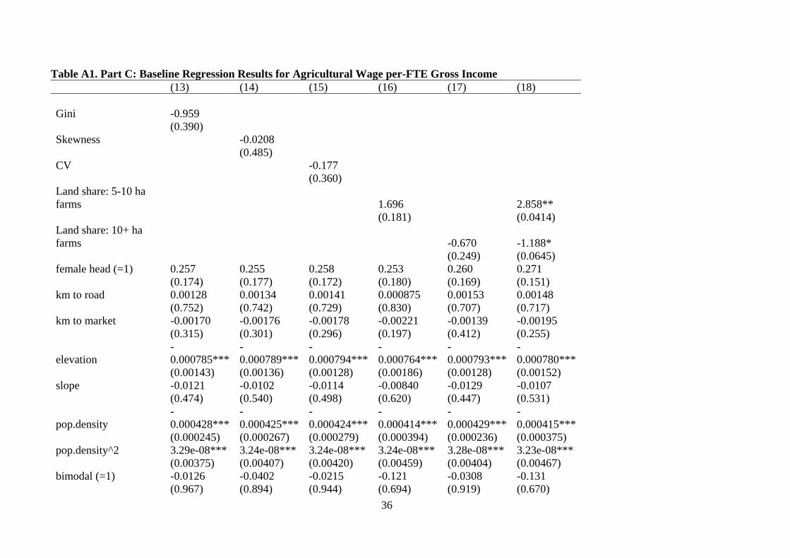
36

Table A1. Part C: Baseline Regression Results for Agricultural Wage per-FTE Gross Income (13) (14) (15) (16) (17) (18) Gini -0.959 (0.390) Skewness -0.0208 (0.485) CV -0.177 (0.360) Land share: 5-10 ha farms 1.696 2.858** (0.181) (0.0414) Land share: 10+ ha farms -0.670 -1.188* (0.249) (0.0645) female head (=1) 0.257 0.255 0.258 0.253 0.260 0.271 (0.174) (0.177) (0.172) (0.180) (0.169) (0.151) km to road 0.00128 0.00134 0.00141 0.000875 0.00153 0.00148 (0.752) (0.742) (0.729) (0.830) (0.707) (0.717) km to market -0.00170 -0.00176 -0.00178 -0.00221 -0.00139 -0.00195 (0.315) (0.301) (0.296) (0.197) (0.412) (0.255)

elevation -0.000785***

-0.000789***

-0.000794***

-0.000764***

-0.000793***

-0.000780***

(0.00143) (0.00136) (0.00128) (0.00186) (0.00128) (0.00152) slope -0.0121 -0.0102 -0.0114 -0.00840 -0.0129 -0.0107 (0.474) (0.540) (0.498) (0.620) (0.447) (0.531)

pop.density -0.000428***

-0.000425***

-0.000424***

-0.000414***

-0.000429***

-0.000415***

(0.000245) (0.000267) (0.000279) (0.000394) (0.000236) (0.000375) pop.density^2 3.29e-08*** 3.24e-08*** 3.24e-08*** 3.24e-08*** 3.28e-08*** 3.23e-08*** (0.00375) (0.00407) (0.00420) (0.00459) (0.00404) (0.00467) bimodal (=1) -0.0126 -0.0402 -0.0215 -0.121 -0.0308 -0.131 (0.967) (0.894) (0.944) (0.694) (0.919) (0.670)

37

(13) (14) (15) (16) (17) (18) 1=region where large farm ASC affects Gini estimates 0.752*** 0.782*** 0.767*** 0.871*** 0.743*** 0.833*** (0.00240) (0.00122) (0.00165) (0.000511) (0.00235) (0.000877) farm size (ha) 0.0119 0.0119 0.0119 0.0118 0.0119 0.0118 (0.480) (0.481) (0.479) (0.485) (0.473) (0.475) age of head 0.00466 0.00454 0.00468 0.00447 0.00426 0.00419 (0.896) (0.899) (0.895) (0.900) (0.905) (0.906) household size 0.140* 0.140* 0.140* 0.140* 0.139* 0.139* (0.0782) (0.0768) (0.0781) (0.0789) (0.0791) (0.0811) max.edu.attainment 0.0714* 0.0714* 0.0711* 0.0718* 0.0716* 0.0715* (0.0834) (0.0833) (0.0847) (0.0818) (0.0821) (0.0828) log(prod.assets) 0.0402 0.0404 0.0429 0.0409 0.0407 0.0411 (0.414) (0.412) (0.384) (0.407) (0.408) (0.404) has ox plough (=1) 0.787* 0.783* 0.783* 0.784* 0.784* 0.783* (0.0607) (0.0616) (0.0621) (0.0618) (0.0615) (0.0624) rainfall (mm) -0.000547 -0.000548 -0.000540 -0.000542 -0.000546 -0.000540 (0.446) (0.445) (0.451) (0.450) (0.446) (0.452) rural (=1) -0.734 -0.722 -0.739 -0.719 -0.721 -0.723 (0.130) (0.135) (0.126) (0.139) (0.136) (0.135) landless (=1) 0.455 0.458 0.484 0.465 0.457 0.474 (0.470) (0.467) (0.442) (0.460) (0.468) (0.452) year==2011 -1.007* -1.007* -1.011* -1.013* -1.006* -1.010* (0.0521) (0.0520) (0.0510) (0.0512) (0.0523) (0.0515) year==2013 -0.702 -0.698 -0.704 -0.701 -0.695 -0.696 (0.186) (0.188) (0.184) (0.187) (0.191) (0.190) zone==2 -2.833*** -2.854*** -2.854*** -2.710*** -2.894*** -2.713*** (5.88e-08) (5.17e-08) (5.32e-08) (4.38e-07) (3.99e-08) (3.96e-07) zone==3 -2.695*** -2.686*** -2.714*** -2.621*** -2.757*** -2.754*** (1.18e-07) (1.21e-07) (1.04e-07) (2.53e-07) (9.64e-08) (1.00e-07) zone==4 -1.289** -1.297** -1.305** -1.383*** -1.289** -1.462*** (0.0121) (0.0116) (0.0112) (0.00695) (0.0117) (0.00452)

38

(13) (14) (15) (16) (17) (18) zone==5 1.124 1.190 1.137 1.372 1.131 1.290 (0.213) (0.183) (0.206) (0.128) (0.207) (0.153) zone==6 -1.043* -1.007* -1.033* -0.973 -1.019* -0.968 (0.0809) (0.0905) (0.0827) (0.103) (0.0869) (0.105) year==2011 & zone==2 1.732*** 1.729*** 1.730*** 1.744*** 1.727*** 1.736*** (0.00933) (0.00943) (0.00940) (0.00902) (0.00947) (0.00915) year==2011 & zone==3 1.465** 1.462** 1.467** 1.463** 1.462** 1.456** (0.0157) (0.0159) (0.0155) (0.0160) (0.0160) (0.0162) year==2011 & zone==4 1.154* 1.162* 1.161* 1.164* 1.155* 1.158* (0.0771) (0.0751) (0.0753) (0.0746) (0.0769) (0.0757) year==2011 & zone==5 2.243** 2.240** 2.244** 2.249** 2.241** 2.245** (0.0383) (0.0386) (0.0381) (0.0379) (0.0385) (0.0381) year==2011 & zone==6 3.654*** 3.658*** 3.662*** 3.649*** 3.656*** 3.649*** (1.19e-07) (1.15e-07) (1.10e-07) (1.27e-07) (1.17e-07) (1.25e-07) year==2013 & zone==2 2.344*** 2.340*** 2.346*** 2.349*** 2.335*** 2.341*** (0.000684) (0.000697) (0.000675) (0.000684) (0.000711) (0.000700) year==2013 & zone==3 1.920*** 1.915*** 1.924*** 1.916*** 1.911*** 1.906*** (0.00150) (0.00153) (0.00146) (0.00155) (0.00159) (0.00164) year==2013 & zone==4 1.997*** 2.002*** 2.002*** 2.004*** 1.995*** 1.999*** (0.00282) (0.00276) (0.00274) (0.00275) (0.00285) (0.00280) year==2013 & zone==5 1.505 1.498 1.502 1.508 1.497 1.501 (0.169) (0.171) (0.169) (0.168) (0.171) (0.170)

39

(13) (14) (15) (16) (17) (18) year==2013 & zone==6 2.507*** 2.507*** 2.514*** 2.499*** 2.501*** 2.494*** (0.000240) (0.000239) (0.000229) (0.000257) (0.000249) (0.000263) Constant 6.178*** 5.777*** 5.945*** 5.337*** 5.873*** 5.405*** (1.68e-09) (0) (0) (8.03e-10) (0) (5.43e-10) Observations 8,540 8,540 8,540 8,540 8,540 8,540 R-squared 0.085 0.085 0.085 0.085 0.085 0.085

Notes: Dependent variables are inverse hyperbolic sine transformed per-FTE gross agricultural wage income measured in 2010 Tanzanian shillings. District-level land concentration measures from 2009 Ag. Sample Census. The regional Gini flag takes a value of one for those regions where the Gini coefficient on land holdings is sensitive to inclusion of the large farm component of the ASC. Dependent variables and other independent control variables are from the NPS. All models include the Mundlak-Chamberlain device. Robust p-values in parentheses, with significance indicated by asterisks: *** p<0.01, ** p<0.05, * p<0.1.

40

Table A1. Part D: Baseline Regression Results for Total per-FTE Gross Income (19) (20) (21) (22) (23) (24) Gini 1.910*** (1.73e-05) Skewness 0.0133 (0.266) CV 0.222*** (0.00528) Land share: 5-10 ha farms 1.666*** 1.658*** (0.000971) (0.00257) Land share: 10+ ha farms 0.306 0.00803 (0.177) (0.974) female head (=1) -0.309*** -0.302*** -0.307*** -0.297*** -0.304*** -0.297*** (0.000402) (0.000550) (0.000446) (0.000665) (0.000504) (0.000672) km to road -0.00324* -0.00296* -0.00322* -0.00306* -0.00305* -0.00307* (0.0502) (0.0735) (0.0516) (0.0635) (0.0652) (0.0627) km to market -0.000858 -0.000800 -0.000754 -0.00130* -0.000961 -0.00130* (0.233) (0.266) (0.295) (0.0733) (0.184) (0.0741) elevation 0.000253*** 0.000246** 0.000255*** 0.000257*** 0.000247** 0.000257*** (0.00948) (0.0123) (0.00932) (0.00858) (0.0117) (0.00869) slope -0.0236*** -0.0262*** -0.0252*** -0.0236*** -0.0248*** -0.0236*** (0.000388) (0.000100) (0.000150) (0.000421) (0.000204) (0.000417) pop.density -3.50e-05 -4.01e-05 -4.05e-05 -3.17e-05 -3.80e-05 -3.15e-05 (0.606) (0.554) (0.552) (0.641) (0.575) (0.643) pop.density^2 4.54e-09 5.04e-09 5.14e-09 4.75e-09 5.01e-09 4.75e-09 (0.446) (0.398) (0.389) (0.425) (0.401) (0.425)

41

(19) (20) (21) (22) (23) (24) bimodal (=1) 0.235* 0.289** 0.261** 0.228* 0.283** 0.229* (0.0752) (0.0284) (0.0475) (0.0858) (0.0321) (0.0848) 1=region where large farm ASC affects Gini estimates -0.0361 -0.104 -0.0787 -0.0371 -0.0880 -0.0369 (0.683) (0.237) (0.371) (0.686) (0.325) (0.687) farm size (ha) 0.00723 0.00727 0.00724 0.00718 0.00723 0.00716 (0.381) (0.373) (0.379) (0.365) (0.367) (0.366) age of head 0.00318 0.00316 0.00327 0.00288 0.00323 0.00294 (0.816) (0.817) (0.810) (0.832) (0.813) (0.829) household size 0.0353 0.0347 0.0350 0.0348 0.0352 0.0348 (0.220) (0.226) (0.223) (0.225) (0.219) (0.225) max.edu.attainment 0.0222 0.0221 0.0222 0.0220 0.0222 0.0220 (0.192) (0.193) (0.190) (0.197) (0.191) (0.197) log(prod.assets) 0.0457* 0.0461* 0.0459* 0.0468** 0.0459* 0.0468** (0.0551) (0.0534) (0.0541) (0.0496) (0.0543) (0.0496) has ox plough (=1) 0.179 0.180 0.181 0.178 0.180 0.178 (0.125) (0.124) (0.121) (0.130) (0.125) (0.129) rainfall (mm) -5.31e-05 -5.20e-05 -5.12e-05 -5.08e-05 -5.25e-05 -5.11e-05 (0.847) (0.850) (0.852) (0.854) (0.849) (0.853) rural (=1) 0.175 0.160 0.169 0.157 0.156 0.156 (0.598) (0.630) (0.612) (0.637) (0.638) (0.639) landless (=1) -0.896** -0.894** -0.895** -0.884** -0.896** -0.885** (0.0141) (0.0144) (0.0142) (0.0157) (0.0142) (0.0156) year==2011 -0.0237 -0.0231 -0.0219 -0.0253 -0.0259 -0.0255 (0.888) (0.891) (0.897) (0.880) (0.878) (0.880) year==2013 0.0946 0.0985 0.0973 0.0963 0.0941 0.0954 (0.570) (0.554) (0.559) (0.562) (0.571) (0.566)

42

(19) (20) (21) (22) (23) (24) zone==2 -0.391* -0.352 -0.339 -0.235 -0.340 -0.235 (0.0948) (0.131) (0.143) (0.315) (0.143) (0.314) zone==3 -0.0428 -0.0882 -0.0468 -0.0611 -0.0655 -0.0605 (0.823) (0.647) (0.806) (0.753) (0.732) (0.752) zone==4 -0.0861 -0.101 -0.0795 -0.213 -0.115 -0.213 (0.606) (0.549) (0.632) (0.204) (0.493) (0.199) zone==5 -0.611* -0.778** -0.695** -0.669** -0.761** -0.670** (0.0558) (0.0153) (0.0294) (0.0392) (0.0177) (0.0383) zone==6 -0.760*** -0.816*** -0.790*** -0.786*** -0.813*** -0.786*** (0.00250) (0.00127) (0.00173) (0.00191) (0.00130) (0.00189) year==2011 & zone==2 -0.0209 -0.0309 -0.0269 -0.0283 -0.0259 -0.0277 (0.945) (0.918) (0.928) (0.925) (0.931) (0.926) year==2011 & zone==3 0.00700 0.0122 0.00890 0.00984 0.0160 0.0105 (0.978) (0.961) (0.972) (0.969) (0.949) (0.967) year==2011 & zone==4 -0.0932 -0.101 -0.0997 -0.0978 -0.0969 -0.0976 (0.667) (0.639) (0.645) (0.651) (0.654) (0.652) year==2011 & zone==5 0.393 0.394 0.393 0.395 0.394 0.395 (0.239) (0.238) (0.239) (0.235) (0.237) (0.235) year==2011 & zone==6 0.544** 0.545** 0.537** 0.547** 0.552** 0.546** (0.0422) (0.0418) (0.0447) (0.0413) (0.0393) (0.0413) year==2013 & zone==2 0.208 0.204 0.206 0.207 0.209 0.208 (0.463) (0.473) (0.469) (0.465) (0.461) (0.463)

43

(19) (20) (21) (22) (23) (24) year==2013 & zone==3 -0.194 -0.191 -0.191 -0.194 -0.186 -0.194 (0.427) (0.434) (0.434) (0.426) (0.445) (0.426) year==2013 & zone==4 -0.117 -0.127 -0.124 -0.122 -0.121 -0.121 (0.573) (0.540) (0.551) (0.558) (0.560) (0.560) year==2013 & zone==5 0.189 0.186 0.188 0.189 0.189 0.190 (0.621) (0.627) (0.624) (0.621) (0.622) (0.620) year==2013 & zone==6 0.455* 0.449* 0.445* 0.453* 0.457* 0.452* (0.0827) (0.0871) (0.0895) (0.0844) (0.0810) (0.0843) Constant 12.26*** 13.15*** 12.92*** 12.86*** 13.13*** 12.86*** (0) (0) (0) (0) (0) (0) Observations 8,540 8,540 8,540 8,540 8,540 8,540 R-squared 0.097 0.095 0.096 0.096 0.095 0.096

Notes: Dependent variables are inverse hyperbolic sine transformed per-FTE gross total income measured in 2010 Tanzanian shillings. District-level land concentration measures from 2009 Ag. Sample Census. The regional Gini flag takes a value of one for those regions where the Gini coefficient on land holdings is sensitive to inclusion of the large farm component of the ASC. Dependent variables and other independent control variables are from the NPS. All models include the Mundlak-Chamberlain device. Robust p-values in parentheses, with significance indicated by asterisks: *** p<0.01, ** p<0.05, * p<0.1.

44

Table A2. Part A: Regression Results for Farm per-FTE Gross Income, Including Interaction Terms between Land Concentration and Asset Terciles

(1) (2) (3) (4) (5) Gini 0.941 (0.299) Gini * medium 1.841*** (0.00526) Gini * wealthy 2.306*** (0.00148) Skewness -0.0780* (0.0766) Skewness * medium 0.111** (0.0144) Skewness * wealthy 0.124*** (0.00789) CV -0.0801 (0.690) CV * medium 0.421** (0.0344) CV * wealthy 0.506** (0.0183) Land share: 5-10 ha farms -2.948* (0.0991) land share * medium 4.876*** (0.00602) land share * wealthy 5.749*** (0.00172)

45

(1) (2) (3) (4) (5) Land share: 10+ ha farms -0.514 (0.387) land share * medium 1.611** (0.0183) land share * wealthy 1.119* (0.0756) female head (=1) -0.102 -0.101 -0.0962 -0.0809 -0.151* (0.326) (0.331) (0.349) (0.434) (0.0803) km to road -0.00202 -0.00174 -0.00200 -0.00131 -0.00130 (0.312) (0.385) (0.312) (0.510) (0.492) km to market 0.00244*** 0.00260*** 0.00259*** 0.00202** 0.00169** (0.00435) (0.00252) (0.00253) (0.0195) (0.0324) elevation 0.000728*** 0.000734*** 0.000736*** 0.000757*** 0.000592*** (7.60e-08) (8.00e-08) (6.07e-08) (1.78e-08) (1.58e-06) slope -0.0335*** -0.0386*** -0.0364*** -0.0355*** -0.0285*** (0.000168) (1.44e-05) (3.24e-05) (6.75e-05) (0.000578) pop.density -0.000413*** -0.000407*** -0.000413*** -0.000393*** -.000138*** (1.86e-06) (2.80e-06) (1.78e-06) (6.58e-06) (0) pop.density^2 1.65e-08*** 1.56e-08** 1.64e-08*** 1.42e-08** 3.07e-09*** (0.00843) (0.0128) (0.00854) (0.0254) (2.16e-09) bimodal (=1) 0.666*** 0.747*** 0.722*** 0.734*** 0.523*** (0.000130) (2.04e-05) (3.10e-05) (3.31e-05) (0.000955) Reg. Gini flag (=1) 0.0634 -0.0329 -0.00638 0.0251 0.0682 (0.585) (0.777) (0.956) (0.834) (0.533) farm size (ha) 0.0185 0.0185* 0.0184 0.0184* 0.0214* (0.104) (0.0971) (0.103) (0.0829) (0.0838) age of head 0.0325** 0.0329** 0.0331** 0.0324** 0.0372** (0.0430) (0.0389) (0.0361) (0.0422) (0.0133)

46

(1) (2) (3) (4) (5) household size 0.0931** 0.0926** 0.0920** 0.0920** 0.104*** (0.0203) (0.0210) (0.0211) (0.0213) (0.00598) max.edu.attainment -0.0285 -0.0289 -0.0286 -0.0288 -0.0264 (0.204) (0.200) (0.201) (0.199) (0.197) log(prod.assets) 0.194*** 0.195*** 0.193*** 0.195*** 0.228*** (1.22e-06) (1.30e-06) (1.45e-06) (1.28e-06) (8.17e-09) has ox plough (=1) 0.224 0.226 0.226 0.226 0.225 (0.170) (0.165) (0.164) (0.164) (0.173) rainfall (mm) -0.000344 -0.000338 -0.000337 -0.000343 -0.000273 (0.340) (0.346) (0.348) (0.340) (0.405) rural (=1) 0.229 0.210 0.226 0.224 0.345 (0.536) (0.569) (0.540) (0.543) (0.314) landless (=1) -6.623*** -6.621*** -6.643*** -6.605*** -6.266*** (0) (0) (0) (0) (0) year==2011 -0.269 -0.267 -0.265 -0.265 -0.341* (0.181) (0.181) (0.182) (0.185) (0.0663) year==2013 -0.511** -0.507** -0.501** -0.513** -0.575*** (0.0275) (0.0278) (0.0287) (0.0261) (0.00408) zone==2 0.216 0.266 0.285 0.386 0.242 (0.493) (0.396) (0.359) (0.219) (0.391) zone==3 0.0629 0.0122 0.0659 0.0192 -0.0684 (0.795) (0.960) (0.783) (0.937) (0.749) zone==4 0.257 0.274 0.298 0.122 0.403** (0.196) (0.169) (0.131) (0.543) (0.0312) zone==5 -1.741*** -1.984*** -1.878*** -1.883*** -1.807*** (3.93e-05) (2.42e-06) (7.04e-06) (1.12e-05) (7.58e-06) zone==6 -1.021*** -1.090*** -1.068*** -1.060*** -0.903*** (0.000192) (8.15e-05) (9.59e-05) (0.000126) (0.000340)

47

year==2011 & zone==2 0.276 0.270 0.269 0.268 0.388 (0.484) (0.494) (0.492) (0.496) (0.295) year==2011 & zone==3 0.168 0.167 0.164 0.165 0.365 (0.560) (0.560) (0.565) (0.567) (0.129) year==2011 & zone==4 -0.178 -0.200 -0.190 -0.185 -0.277 (0.496) (0.443) (0.463) (0.478) (0.263) year==2011 & zone==5 1.351*** 1.344*** 1.332*** 1.341*** 1.415*** (0.00217) (0.00224) (0.00230) (0.00237) (0.000878) year==2011 & zone==6 0.208 0.202 0.199 0.196 0.264 (0.478) (0.488) (0.492) (0.503) (0.325) year==2013 & zone==2 0.214 0.211 0.206 0.218 0.196 (0.618) (0.625) (0.630) (0.613) (0.608) year==2013 & zone==3 0.209 0.205 0.205 0.214 0.456* (0.505) (0.512) (0.510) (0.495) (0.0715) year==2013 & zone==4 0.167 0.145 0.148 0.168 0.0890 (0.547) (0.601) (0.590) (0.545) (0.727) year==2013 & zone==5 1.641*** 1.625*** 1.617*** 1.632*** 1.634*** (0.000893) (0.000964) (0.000937) (0.000956) (0.000466) year==2013 & zone==6 0.684** 0.668** 0.659** 0.674** 0.722*** (0.0262) (0.0293) (0.0307) (0.0280) (0.00720) Constant 5.853*** 6.714*** 6.530*** 6.580*** 6.292*** (0) (0) (0) (0) (0) Observations 8,540 8,540 8,540 8,540 11,791 R-squared 0.557 0.555 0.557 0.556 0.693

Notes: Dependent variables are inverse hyperbolic sine transformed per-FTE gross farm income measured in 2010 Tanzanian shillings. District-level land concentration measures from 2009 Ag. Sample Census. The regional Gini flag takes a value of one for those regions where the Gini coefficient on land holdings is sensitive to inclusion of the large farm component of the ASC. Dependent variables and other independent control variables are from the NPS. The harvest incomplete dummy receives a value of 1 for households which report one or more fields had not been harvested at the time of enumeration. All models include the Mundlak-Chamberlain device. Robust p-values in parentheses, with significance indicated by asterisks: *** p<0.01, ** p<0.05, * p<0.1.

48

Table A2. Part B: Regression Results for Non-farm per-FTE Gross Income, Including Interaction Terms between Land Concentration and Asset Terciles

(6) (7) (8) (9) (10) Gini -0.0621

(0.962) Gini * medium 1.713** (0.0268) Gini * wealthy 1.782* (0.0596) Skewness -0.103** (0.0488) Skewness * medium 0.140*** (0.00975) Skewness * wealthy 0.145** (0.0197) CV -0.339 (0.167) CV * medium 0.603** (0.0100) CV * wealthy 0.624** (0.0281) Land share: 5-10 ha farms 2.817 (0.224) land share * medium 2.049 (0.358) land share * wealthy 1.573 (0.530)

49

(6) (7) (8) (9) (10) Land share: 10+ ha farms -1.048 (0.183) land share * medium 1.432 (0.133) land share * wealthy 0.141 (0.887) female head (=1) -0.138 -0.135 -0.138 -0.125 -0.297* (0.489) (0.497) (0.488) (0.531) (0.0685) km to road -0.00597 -0.00591 -0.00598 -0.00606 -0.00643 (0.165) (0.171) (0.165) (0.159) (0.107) km to market -0.00347* -0.00342* -0.00348* -0.00467** -0.00275* (0.0525) (0.0570) (0.0534) (0.0103) (0.0872) elevation -0.000667** -0.000683** -0.000671** -0.000637** -0.000522** (0.0150) (0.0127) (0.0143) (0.0200) (0.0318) slope -0.0538*** -0.0563*** -0.0546*** -0.0504*** -0.0554*** (0.00249) (0.00149) (0.00210) (0.00446) (0.000699) pop.density 0.000118 0.000127 0.000119 0.000149 4.44e-06 (0.321) (0.284) (0.319) (0.213) (0.864) pop.density^2 -1.83e-09 -3.32e-09 -2.27e-09 -3.52e-09 5.44e-10 (0.846) (0.724) (0.809) (0.711) (0.414) bimodal (=1) -0.487 -0.475 -0.482 -0.607* -0.242 (0.141) (0.151) (0.144) (0.0700) (0.405) Reg. Gini flag (=1) 0.730*** 0.701*** 0.709*** 0.875*** 0.443** (0.00334) (0.00428) (0.00402) (0.000588) (0.0451) farm size (ha) -0.00167 -0.00180 -0.00177 -0.00181 -0.00205 (0.937) (0.933) (0.934) (0.932) (0.925) age of head -0.0230 -0.0230 -0.0229 -0.0235 -0.0215 (0.527) (0.527) (0.529) (0.517) (0.502)

50

(6) (7) (8) (9) (10) household size 0.186** 0.186** 0.186** 0.185** 0.183** (0.0227) (0.0222) (0.0221) (0.0239) (0.0132) max.edu.attainment 0.186*** 0.185*** 0.185*** 0.186*** 0.161*** (2.82e-05) (3.03e-05) (2.99e-05) (2.88e-05) (1.11e-05) log(prod.assets) 0.0256 0.0242 0.0239 0.0262 0.00698 (0.628) (0.647) (0.650) (0.620) (0.889) has ox plough (=1) 1.157*** 1.152*** 1.153*** 1.154*** 1.135*** (0.00572) (0.00604) (0.00594) (0.00592) (0.00640) rainfall (mm) -0.000123 -0.000129 -0.000127 -0.000123 -0.000280 (0.863) (0.858) (0.859) (0.864) (0.659) rural (=1) -0.433 -0.422 -0.427 -0.427 -0.654 (0.413) (0.422) (0.418) (0.419) (0.189) landless (=1) 1.038* 1.023* 1.027* 1.033* 0.502 (0.0851) (0.0894) (0.0883) (0.0865) (0.361) year==2011 0.00806 0.00823 0.0143 -0.00605 0.150 (0.988) (0.988) (0.979) (0.991) (0.763) year==2013 0.0336 0.0413 0.0465 0.0219 0.0407 (0.951) (0.940) (0.933) (0.968) (0.932) zone==2 -3.585*** -3.574*** -3.560*** -3.251*** -3.283*** (1.28e-08) (1.38e-08) (1.64e-08) (3.86e-07) (1.37e-08) zone==3 -1.494*** -1.517*** -1.492*** -1.444*** -1.253** (0.00727) (0.00628) (0.00735) (0.00950) (0.0116) zone==4 -0.941* -0.933* -0.931 -1.201** -0.736 (0.0965) (0.0988) (0.100) (0.0346) (0.150) zone==5 2.030** 1.957** 1.990** 2.254*** 1.567** (0.0134) (0.0160) (0.0147) (0.00598) (0.0381) zone==6 -0.212 -0.220 -0.226 -0.141 -0.175 (0.743) (0.734) (0.727) (0.828) (0.762)

51

(6) (7) (8) (9) (10) year==2011 & zone==2 2.031** 2.037** 2.026** 2.053** 1.808** (0.0117) (0.0113) (0.0118) (0.0109) (0.0138) year==2011 & zone==3 0.863 0.862 0.858 0.865 0.485 (0.201) (0.201) (0.204) (0.199) (0.394) year==2011 & zone==4 0.745 0.735 0.734 0.760 0.514 (0.301) (0.307) (0.308) (0.290) (0.432) year==2011 & zone==5 1.497* 1.496* 1.488* 1.497* 1.357* (0.0880) (0.0882) (0.0901) (0.0877) (0.0991) year==2011 & zone==6 2.815*** 2.805*** 2.797*** 2.819*** 2.401*** (8.80e-05) (9.27e-05) (9.86e-05) (8.47e-05) (0.000209) year==2013 & zone==2 2.864*** 2.870*** 2.859*** 2.882*** 2.701*** (0.000348) (0.000326) (0.000351) (0.000322) (0.000137) year==2013 & zone==3 0.787 0.777 0.775 0.798 0.658 (0.229) (0.235) (0.237) (0.223) (0.221) year==2013 & zone==4 0.888 0.870 0.870 0.908 0.919 (0.215) (0.224) (0.224) (0.205) (0.143) year==2013 & zone==5 0.491 0.483 0.476 0.491 0.543 (0.603) (0.609) (0.614) (0.603) (0.526) year==2013 & zone==6 1.923*** 1.902*** 1.900*** 1.923*** 1.716*** (0.00686) (0.00748) (0.00753) (0.00687) (0.00569) Constant 15.10*** 15.64*** 15.55*** 14.51*** 14.87*** (0) (0) (0) (0) (0) Observations 8,540 8,540 8,540 8,540 11,791 R-squared 0.167 0.167 0.167 0.168 0.194

Notes: Dependent variables are inverse hyperbolic sine transformed per-FTE gross non-farm income measured in 2010 Tanzanian shillings. District-level land concentration measures from 2009 Ag. Sample Census. The regional Gini flag takes a value of one for those regions where the Gini coefficient on land holdings is sensitive to inclusion of the large farm component of the ASC. Dependent variables and other independent control variables are from the NPS. All models include the Mundlak-Chamberlain device. Robust p-values in parentheses, with significance indicated by asterisks: *** p<0.01, ** p<0.05, * p<0.1.

52

Table A2. Part C: Regression Results for Agricultural Wage per-FTE Gross Income, Including Interaction Terms between Land Concentration and Asset Terciles (11) (12) (13) (14) (15) Gini -1.873 (0.143) Gini * medium 2.020*** (0.00953) Gini * wealthy 0.843 (0.359) Skewness -0.0798* (0.0922) Skewness * medium 0.137*** (0.00739) Skewness * wealthy 0.0219 (0.693) CV -0.422* (0.0763) CV * medium 0.606*** (0.00801) CV * wealthy 0.147 (0.578) Land share: 5-10 ha farms -3.399 (0.123) land share * medium 7.237*** (0.000716) land share * wealthy 4.596* (0.0509) Land share: 10+ ha farms -2.120***

53

(11) (12) (13) (14) (15) (0.00140) land share * medium 2.606*** (0.00228) land share * wealthy 1.496* (0.0763) female head (=1) 0.202 0.200 0.201 0.220 0.308** (0.289) (0.292) (0.290) (0.247) (0.0434) km to road 0.00185 0.00202 0.00193 0.00159 0.00295 (0.650) (0.620) (0.636) (0.696) (0.432) km to market -0.00183 -0.00181 -0.00181 -0.00231 -0.00243 (0.280) (0.289) (0.289) (0.178) (0.105) elevation -0.000684*** -0.000683*** -0.000696*** -0.000678*** -0.000791*** (0.00567) (0.00571) (0.00486) (0.00602) (0.000279) slope -0.0146 -0.0137 -0.0141 -0.0106 -0.00600 (0.385) (0.409) (0.400) (0.532) (0.699) pop.density -0.000432*** -0.000422*** -0.000423*** -0.000412*** -7.95e-05*** (0.000224) (0.000303) (0.000296) (0.000427) (0.000123) pop.density^2 3.37e-08*** 3.21e-08*** 3.25e-08*** 3.11e-08*** 2.10e-09*** (0.00311) (0.00430) (0.00406) (0.00621) (2.66e-05) bimodal (=1) 0.00910 -0.0171 -0.0136 -0.0985 -0.241 (0.976) (0.955) (0.964) (0.748) (0.361) Reg. Gini flag (=1) 0.757*** 0.773*** 0.772*** 0.884*** 0.763*** (0.00219) (0.00135) (0.00149) (0.000415) (0.000435) farm size (ha) 0.0118 0.0118 0.0118 0.0116 0.00894 (0.468) (0.472) (0.470) (0.476) (0.561) age of head 0.00460 0.00492 0.00479 0.00456 0.00764 (0.897) (0.890) (0.893) (0.898) (0.806) household size 0.140* 0.140* 0.140* 0.139* 0.153**

54

(11) (12) (13) (14) (15) (0.0792) (0.0779) (0.0786) (0.0799) (0.0332) max.edu.attainment 0.0710* 0.0704* 0.0704* 0.0715* 0.0533 (0.0855) (0.0879) (0.0881) (0.0835) (0.106) log(prod.assets) 0.0431 0.0409 0.0432 0.0436 0.0397 (0.380) (0.404) (0.380) (0.375) (0.379) has ox plough (=1) 0.782* 0.783* 0.780* 0.780* 0.752* (0.0618) (0.0612) (0.0625) (0.0626) (0.0685) rainfall (mm) -0.000546 -0.000544 -0.000540 -0.000544 -0.000831 (0.446) (0.446) (0.450) (0.449) (0.190) rural (=1) -0.730 -0.706 -0.734 -0.701 -0.528 (0.130) (0.142) (0.127) (0.145) (0.245) landless (=1) 0.500 0.484 0.504 0.507 0.558 (0.426) (0.441) (0.423) (0.421) (0.308) year==2011 -1.015** -1.013* -1.012* -1.019** -0.887* (0.0499) (0.0501) (0.0503) (0.0493) (0.0533) year==2013 -0.702 -0.700 -0.698 -0.707 -0.683 (0.185) (0.187) (0.187) (0.183) (0.127) zone==2 -2.781*** -2.791*** -2.787*** -2.679*** -2.730*** (9.96e-08) (9.84e-08) (1.04e-07) (6.01e-07) (6.16e-09) zone==3 -2.624*** -2.589*** -2.624*** -2.577*** -2.327*** (2.36e-07) (3.20e-07) (2.52e-07) (3.90e-07) (3.47e-07) zone==4 -1.227** -1.200** -1.222** -1.355*** -1.090** (0.0167) (0.0195) (0.0174) (0.00817) (0.0160) zone==5 1.087 1.147 1.132 1.351 1.542* (0.228) (0.199) (0.207) (0.135) (0.0624) zone==6 -1.077* -0.996* -1.018* -0.972 -0.631 (0.0709) (0.0934) (0.0866) (0.103) (0.229) year==2011 & zone==2 1.716*** 1.716*** 1.715*** 1.728*** 1.545***

55

(11) (12) (13) (14) (15) (0.00992) (0.00979) (0.00993) (0.00963) (0.00947) year==2011 & zone==3 1.477** 1.472** 1.473** 1.471** 1.186** (0.0148) (0.0150) (0.0150) (0.0153) (0.0201) year==2011 & zone==4 1.154* 1.162* 1.155* 1.168* 1.073* (0.0770) (0.0749) (0.0765) (0.0736) (0.0672) year==2011 & zone==5 2.280** 2.272** 2.268** 2.290** 1.828* (0.0353) (0.0356) (0.0361) (0.0347) (0.0732) year==2011 & zone==6 3.652*** 3.654*** 3.648*** 3.633*** 3.222*** (1.15e-07) (1.13e-07) (1.18e-07) (1.39e-07) (1.65e-07) year==2013 & zone==2 2.325*** 2.324*** 2.324*** 2.340*** 2.414*** (0.000725) (0.000732) (0.000726) (0.000700) (5.79e-05) year==2013 & zone==3 1.930*** 1.920*** 1.923*** 1.930*** 1.629*** (0.00139) (0.00148) (0.00145) (0.00142) (0.000942) year==2013 & zone==4 1.997*** 2.003*** 1.996*** 2.013*** 1.873*** (0.00279) (0.00273) (0.00280) (0.00260) (0.00114) year==2013 & zone==5 1.534 1.526 1.520 1.542 1.632 (0.160) (0.162) (0.164) (0.159) (0.101) year==2013 & zone==6 2.504*** 2.508*** 2.502*** 2.488*** 2.340*** (0.000237) (0.000235) (0.000240) (0.000267) (5.89e-05) Constant 5.596*** 5.107*** 5.287*** 5.136*** 5.398*** (1.98e-07) (3.91e-09) (7.06e-09) (1.46e-08) (0) Observations 8,540 8,540 8,540 8,540 11,791 R-squared 0.087 0.087 0.087 0.087 0.107

Notes: Dependent variables are inverse hyperbolic sine transformed per-FTE gross agricultural wage income measured in 2010 Tanzanian shillings. District-level land concentration measures from 2009 Ag. Sample Census. The regional Gini flag takes a value of one for those regions where the Gini coefficient on land holdings is sensitive to inclusion of the large farm component of the ASC. Dependent variables and other independent control variables are from the NPS. All models include the Mundlak-Chamberlain device. Robust p-values in parentheses, with significance indicated by asterisks: *** p<0.01, ** p<0.05, * p<0.1.

56

Table A2. Part D: Regression Results for Total per-FTE Gross Income, Including Interaction Terms between Land Concentration and Asset Terciles (16) (17) (18) (19) (20) Gini 1.505** (0.0126) Gini * medium 0.183 (0.674) Gini * wealthy 0.661 (0.166) Skewness -0.0506 (0.266) Skewness * medium 0.0503 (0.243) Skewness * wealthy 0.0891* (0.0517) CV 0.0879 (0.587) CV * medium 0.0719 (0.627) CV * wealthy 0.226 (0.165) Land share: 5-10 ha farms 1.105 (0.481) land share * medium 0.0432 (0.977) land share * wealthy 0.987 (0.531) Land share: 10+ ha farms -0.370 (0.546) land share * medium 0.593 (0.345)

57

(16) (17) (18) (19) (20) land share * wealthy 0.794 (0.214) female head (=1) -0.292*** -0.289*** -0.293*** -0.284*** -0.424*** (0.000855) (0.000960) (0.000846) (0.00113) (6.96e-08) km to road -0.00340** -0.00315* -0.00339** -0.00308* -0.00318** (0.0393) (0.0567) (0.0408) (0.0568) (0.0438) km to market -0.000870 -0.000848 -0.000816 -0.00130* -0.000998 (0.225) (0.238) (0.256) (0.0730) (0.127) elevation 0.000224** 0.000219** 0.000231** 0.000240** 0.000275*** (0.0228) (0.0269) (0.0197) (0.0146) (0.00403) slope -0.0224*** -0.0251*** -0.0240*** -0.0230*** -0.0225*** (0.000753) (0.000188) (0.000305) (0.000538) (0.000345) pop.density -3.73e-05 -3.98e-05 -4.25e-05 -2.89e-05 1.63e-05 (0.582) (0.556) (0.531) (0.671) (0.366) pop.density^2 4.60e-09 4.53e-09 5.09e-09 4.33e-09 3.26e-10 (0.440) (0.448) (0.393) (0.471) (0.509) bimodal (=1) 0.218* 0.264** 0.248* 0.231* 0.235* (0.0998) (0.0479) (0.0611) (0.0802) (0.0636) Reg. Gini flag (=1) -0.0311 -0.0919 -0.0737 -0.0391 -0.124 (0.725) (0.302) (0.404) (0.669) (0.149) farm size (ha) 0.00724 0.00722 0.00722 0.00722 0.00699 (0.384) (0.385) (0.384) (0.359) (0.364) age of head 0.00310 0.00309 0.00328 0.00286 0.00141 (0.820) (0.821) (0.810) (0.833) (0.910) household size 0.0353 0.0354 0.0352 0.0348 0.0439 (0.219) (0.219) (0.221) (0.225) (0.110) max.edu.attainment 0.0224 0.0220 0.0223 0.0222 0.0253 (0.187) (0.193) (0.188) (0.192) (0.115) log(prod.assets) 0.0457* 0.0467** 0.0461* 0.0461* 0.0296 (0.0546) (0.0487) (0.0532) (0.0534) (0.183) has ox plough (=1) 0.180 0.178 0.181 0.181 0.235** (0.125) (0.130) (0.122) (0.123) (0.0470)

58

(16) (17) (18) (19) (20) rainfall (mm) -5.39e-05 -5.10e-05 -5.13e-05 -5.11e-05 -9.43e-05 (0.845) (0.852) (0.852) (0.853) (0.719) rural (=1) 0.175 0.161 0.168 0.164 0.209 (0.599) (0.625) (0.613) (0.625) (0.516) landless (=1) -0.896** -0.887** -0.895** -0.891** -1.054*** (0.0141) (0.0154) (0.0143) (0.0150) (0.00158) year==2011 -0.0227 -0.0215 -0.0215 -0.0230 0.0822 (0.893) (0.899) (0.899) (0.891) (0.641) year==2013 0.0972 0.105 0.101 0.0981 0.137 (0.560) (0.530) (0.545) (0.555) (0.429) zone==2 -0.402* -0.371 -0.357 -0.250 -0.266 (0.0861) (0.112) (0.125) (0.285) (0.282) zone==3 -0.0577 -0.106 -0.0619 -0.0732 -0.0143 (0.762) (0.584) (0.746) (0.705) (0.941) zone==4 -0.121 -0.139 -0.111 -0.232 -0.0513 (0.474) (0.410) (0.507) (0.168) (0.773) zone==5 -0.588* -0.751** -0.681** -0.657** -0.782** (0.0664) (0.0196) (0.0332) (0.0433) (0.0126) zone==6 -0.757*** -0.817*** -0.802*** -0.788*** -0.669*** (0.00258) (0.00122) (0.00155) (0.00187) (0.00738) year==2011 & zone==2 -0.0194 -0.0334 -0.0262 -0.0248 -0.0393 (0.948) (0.911) (0.931) (0.934) (0.896) year==2011 & zone==3 0.00552 0.00746 0.00640 0.00627 -0.121 (0.982) (0.976) (0.980) (0.980) (0.608) year==2011 & zone==4 -0.0915 -0.107 -0.0999 -0.0956 -0.296 (0.673) (0.620) (0.644) (0.658) (0.184) year==2011 & zone==5 0.395 0.398 0.394 0.392 0.341 (0.237) (0.234) (0.238) (0.240) (0.296) year==2011 & zone==6 0.543** 0.539** 0.535** 0.546** 0.361 (0.0425) (0.0434) (0.0452) (0.0415) (0.162) year==2013 & zone==2 0.211 0.201 0.206 0.211 0.153 (0.457) (0.478) (0.467) (0.458) (0.597)

59

(16) (17) (18) (19) (20) year==2013 & zone==3 -0.198 -0.205 -0.198 -0.196 -0.165 (0.417) (0.399) (0.415) (0.421) (0.462) year==2013 & zone==4 -0.119 -0.139 -0.129 -0.122 -0.142 (0.566) (0.502) (0.533) (0.559) (0.501) year==2013 & zone==5 0.189 0.183 0.184 0.184 0.170 (0.622) (0.633) (0.631) (0.632) (0.633) year==2013 & zone==6 0.452* 0.435* 0.438* 0.450* 0.263 (0.0839) (0.0942) (0.0928) (0.0854) (0.294) Constant 12.67*** 13.58*** 13.28*** 13.09*** 13.14*** (0) (0) (0) (0) (0) Observations 8,540 8,540 8,540 8,540 11,791 R-squared 0.098 0.097 0.097 0.097 0.090

Notes: Dependent variables are inverse hyperbolic sine transformed per-FTE gross total income measured in 2010 Tanzanian shillings. District-level land concentration measures from 2009 Ag. Sample Census. The regional Gini flag takes a value of one for those regions where the Gini coefficient on land holdings is sensitive to inclusion of the large farm component of the ASC. Dependent variables and other independent control variables are from the NPS. All models include the Mundlak-Chamberlain device. Robust p-values in parentheses, with significance indicated by asterisks: *** p<0.01, ** p<0.05, * p<0.1.

60

Table A3. Part A: Inter-period Income Changes Regressed on Lagged Independent Variables: Farm per-FTE Gross Income (1) (2) (3) (4) (5) (6) Gini 1.852 (0.214) Skewness 0.0321 (0.353) CV 0.339 (0.175) Land share: 5-10 ha farms 2.689* 2.718 (0.0990) (0.144) Land share: 10+ ha farms 0.481 -0.0283 (0.507) (0.973) lag: farm size (ha) 0.0415* 0.0409* 0.0424* 0.0346 0.0397* 0.0345 (0.0612) (0.0649) (0.0578) (0.111) (0.0709) (0.110) lag: age of head 0.150** 0.149** 0.148** 0.151** 0.152** 0.151** (0.0154) (0.0164) (0.0168) (0.0152) (0.0146) (0.0151) lag: household size 0.0965 0.0966 0.102 0.0885 0.0942 0.0883 (0.481) (0.480) (0.457) (0.516) (0.491) (0.516) lag: max.edu.attainment -0.0132 -0.0134 -0.0147 -0.0129 -0.0123 -0.0129 (0.829) (0.828) (0.812) (0.834) (0.841) (0.834) lag: log(prod.assets) -0.117 -0.118 -0.116 -0.115 -0.117 -0.115 (0.172) (0.169) (0.177) (0.181) (0.175) (0.180) lag: has ox plough (=1) -1.191** -1.180** -1.182** -1.189** -1.192** -1.188** (0.0178) (0.0186) (0.0186) (0.0179) (0.0178) (0.0180) lag: rainfall (mm) 0.00175** 0.00179** 0.00177** 0.00154* 0.00175** 0.00154* (0.0365) (0.0311) (0.0343) (0.0728) (0.0366) (0.0727) lag: rural (=1) 3.933*** 3.933*** 3.917*** 3.976*** 3.964*** 3.976***

61

(1) (2) (3) (4) (5) (6) (0.00680) (0.00685) (0.00713) (0.00599) (0.00630) (0.00601) lag: landless (=1) -1.446 -1.430 -1.479 -1.334 -1.403 -1.334 (0.346) (0.350) (0.335) (0.383) (0.359) (0.383) lag: female head (=1) -0.247 -0.244 -0.247 -0.234 -0.244 -0.233 (0.349) (0.353) (0.347) (0.373) (0.355) (0.376) lag: km to road -0.00444 -0.00436 -0.00453 -0.00432 -0.00436 -0.00430 (0.381) (0.391) (0.372) (0.392) (0.391) (0.397) lag: km to market -0.00335 -0.00321 -0.00322 -0.00394 -0.00350 -0.00394 (0.163) (0.184) (0.182) (0.101) (0.144) (0.101) lag: elevation 0.000269 0.000282 0.000277 0.000269 0.000275 0.000268 (0.395) (0.372) (0.381) (0.395) (0.385) (0.395) lag: slope 0.0164 0.0134 0.0153 0.0180 0.0159 0.0179 (0.365) (0.458) (0.395) (0.322) (0.381) (0.325) lag: pop.density 0.000138 0.000142 0.000137 0.000149 0.000139 0.000149 (0.305) (0.293) (0.310) (0.268) (0.301) (0.268) lag: pop.density^2 1.50e-09 1.46e-09 1.57e-09 1.25e-09 1.53e-09 1.24e-09 (0.747) (0.751) (0.734) (0.787) (0.740) (0.788) lag: bimodal (=1) -0.446 -0.395 -0.434 -0.488 -0.398 -0.489 (0.292) (0.344) (0.301) (0.244) (0.341) (0.243) lag: Reg. Gini flag (=1) 0.315 0.256 0.286 0.374 0.278 0.373 (0.288) (0.377) (0.328) (0.215) (0.353) (0.219) zone==2 0.0974 0.143 0.157 0.348 0.159 0.348 (0.835) (0.758) (0.733) (0.464) (0.731) (0.464) zone==3 0.269 0.254 0.298 0.281 0.279 0.278 (0.478) (0.502) (0.428) (0.464) (0.470) (0.471) zone==4 0.124 0.128 0.156 -0.0820 0.0926 -0.0842 (0.715) (0.709) (0.648) (0.815) (0.786) (0.809) zone==5 2.155*** 2.029*** 2.137*** 2.143*** 2.023*** 2.141*** (0.00172) (0.00256) (0.00159) (0.00174) (0.00275) (0.00169) zone==6 1.392*** 1.327** 1.370*** 1.336*** 1.330*** 1.336***

62

(1) (2) (3) (4) (5) (6) (0.00702) (0.0101) (0.00776) (0.00969) (0.00982) (0.00962) Constant -3.158** -2.382** -2.673** -2.810** -2.367** -2.809** (0.0221) (0.0454) (0.0281) (0.0236) (0.0475) (0.0239) Observations 2,397 2,397 2,397 2,397 2,397 2,397 R-squared 0.041 0.040 0.041 0.041 0.040 0.041

Notes: Dependent variables are the change in the inverse hyperbolic sine transformed per-FTE gross farm income, regressed against lagged independent variables. All values measured in real 2010 Tanzanian shillings. District-level land concentration measures from 2009 Ag. Sample Census. The regional Gini flag takes a value of one for those regions where the Gini coefficient on land holdings is sensitive to inclusion of the large farm component of the ASC. Dependent variables and other independent control variables are from the NPS. All models include the Mundlak-Chamberlain device. Robust p-values in parentheses, with significance indicated by asterisks: *** p<0.01, ** p<0.05, * p<0.1.

63

Table A3. Part B: Inter-period Income Changes Regressed on Lagged Independent Variables: Non-farm per-FTE Gross Income (7) (8) (9) (10) (11) (12) Gini 3.401 (0.236) Skewness 0.0756 (0.322) CV 0.470 (0.281) Land share: 5-10 ha farms 2.601 -0.191 (0.442) (0.959) Land share: 10+ ha farms 2.694* 2.730 (0.0783) (0.104) lag: farm size (ha) -0.0270 -0.0273 -0.0266 -0.0354 -0.0292 -0.0288 (0.761) (0.757) (0.764) (0.691) (0.744) (0.749) lag: age of head 0.223 0.221 0.222 0.226 0.229 0.229 (0.159) (0.166) (0.163) (0.157) (0.146) (0.146) lag: household size -0.474* -0.471* -0.469* -0.486* -0.469* -0.468* (0.0576) (0.0591) (0.0603) (0.0522) (0.0594) (0.0596) lag: max.edu.attainment 0.00967 0.00860 0.00822 0.0111 0.00987 0.00991 (0.934) (0.941) (0.944) (0.924) (0.933) (0.933) lag: log(prod.assets) -0.0770 -0.0781 -0.0756 -0.0761 -0.0672 -0.0673 (0.554) (0.549) (0.561) (0.559) (0.605) (0.604) lag: has ox plough (=1) -0.200 -0.175 -0.184 -0.194 -0.218 -0.218 (0.856) (0.873) (0.867) (0.861) (0.843) (0.843)

lag: rainfall (mm) -0.00572*** -0.00563*** -0.00569*** -0.00590*** -0.00581***

-0.00580***

(0.000594) (0.000773) (0.000654) (0.000486) (0.000507) (0.000654)

64

(7) (8) (9) (10) (11) (12) lag: rural (=1) -2.663* -2.682* -2.671* -2.593 -2.618 -2.619 (0.0984) (0.0946) (0.0968) (0.108) (0.105) (0.105) lag: landless (=1) -2.611 -2.588 -2.643 -2.477 -2.478 -2.483 (0.105) (0.106) (0.101) (0.123) (0.124) (0.125) lag: female head (=1) 1.163** 1.166** 1.167** 1.184** 1.145** 1.144** (0.0194) (0.0194) (0.0191) (0.0172) (0.0215) (0.0216) lag: km to road 0.0136 0.0136 0.0136 0.0140 0.0127 0.0127 (0.210) (0.209) (0.209) (0.196) (0.241) (0.241) lag: km to market -0.00503 -0.00475 -0.00480 -0.00551 -0.00622 -0.00619 (0.265) (0.294) (0.290) (0.228) (0.167) (0.172) lag: elevation -0.000375 -0.000345 -0.000363 -0.000374 -0.000350 -0.000350 (0.554) (0.585) (0.565) (0.555) (0.579) (0.580) lag: slope 0.0410 0.0349 0.0386 0.0409 0.0455 0.0453 (0.359) (0.430) (0.385) (0.361) (0.310) (0.313) lag: pop.density -0.000225 -0.000218 -0.000227 -0.000214 -0.000221 -0.000222 (0.186) (0.202) (0.183) (0.215) (0.194) (0.194) lag: pop.density^2 3.24e-09 3.13e-09 3.36e-09 3.03e-09 3.26e-09 3.28e-09 (0.634) (0.648) (0.624) (0.661) (0.635) (0.633) lag: bimodal (=1) 0.967 1.055 1.010 0.978 1.001 1.008 (0.211) (0.171) (0.190) (0.210) (0.190) (0.195) lag: Reg. Gini flag (=1) -1.441** -1.542*** -1.516*** -1.449** -1.367** -1.374** (0.0152) (0.00826) (0.00949) (0.0185) (0.0202) (0.0249) zone==2 2.366** 2.462*** 2.459** 2.627*** 2.634*** 2.620*** (0.0129) (0.00993) (0.0103) (0.00862) (0.00650) (0.00855) zone==3 1.440* 1.431* 1.456* 1.405* 1.695** 1.695** (0.0592) (0.0578) (0.0564) (0.0653) (0.0334) (0.0334) zone==4 1.008 1.036 1.034 0.776 0.968 0.980 (0.195) (0.180) (0.185) (0.322) (0.208) (0.219) zone==5 -0.925 -1.118 -1.044 -1.116 -0.892 -0.901 (0.461) (0.358) (0.398) (0.366) (0.465) (0.466)

65

(7) (8) (9) (10) (11) (12) zone==6 0.849 0.731 0.789 0.737 0.754 0.753 (0.412) (0.476) (0.444) (0.472) (0.462) (0.463) Constant -1.496 -0.142 -0.416 -0.369 -0.492 -0.461 (0.558) (0.945) (0.846) (0.866) (0.815) (0.833) Observations 2,397 2,397 2,397 2,397 2,397 2,397 R-squared 0.038 0.038 0.038 0.038 0.039 0.039

Notes: Dependent variables are the change in the inverse hyperbolic sine transformed per-FTE gross non-farm income, regressed against lagged independent variables. All values measured in real 2010 Tanzanian shillings. District-level land concentration measures from 2009 Ag. Sample Census. The regional Gini flag takes a value of one for those regions where the Gini coefficient on land holdings is sensitive to inclusion of the large farm component of the ASC. Dependent variables and other independent control variables are from the NPS. All models include the Mundlak-Chamberlain device. Robust p-values in parentheses, with significance indicated by asterisks: *** p<0.01, ** p<0.05, * p<0.1.

66

Table A3. Part C: Inter-Period Income Changes Regressed On Lagged Independent Variables: Agricultural Wage Per-FTE Gross Income (13) (14) (15) (16) (17) (18) Gini 2.694 (0.316) Skewness -0.0787 (0.268) CV 0.0890 (0.837) Land share: 5-10 ha farms 2.089 -0.352 (0.519) (0.921) Land share: 10+ ha farms 2.320 2.386 (0.109) (0.131) lag: farm size (ha) -0.0339 -0.0404 -0.0360 -0.0406 -0.0355 -0.0348 (0.587) (0.517) (0.563) (0.517) (0.568) (0.578) lag: age of head 0.225 0.233 0.227 0.227 0.230 0.230 (0.140) (0.124) (0.135) (0.135) (0.131) (0.131) lag: household size -0.188 -0.207 -0.192 -0.197 -0.183 -0.182 (0.400) (0.354) (0.391) (0.375) (0.413) (0.415) lag: max.edu.attainment 0.0102 0.0156 0.0114 0.0114 0.0102 0.0103 (0.924) (0.885) (0.916) (0.916) (0.925) (0.924) lag: log(prod.assets) -0.0133 -0.0170 -0.0147 -0.0126 -0.00475 -0.00492 (0.908) (0.884) (0.899) (0.914) (0.967) (0.966) lag: has ox plough (=1) -0.418 -0.430 -0.411 -0.413 -0.434 -0.435 (0.687) (0.677) (0.692) (0.691) (0.676) (0.675) lag: rainfall (mm) -0.00388** -0.00390** -0.00385** -0.00403** -0.00396** -0.00394** (0.0165) (0.0161) (0.0174) (0.0140) (0.0148) (0.0173) lag: rural (=1) -1.792 -1.659 -1.756 -1.737 -1.757 -1.759 (0.255) (0.287) (0.263) (0.268) (0.267) (0.267) lag: landless (=1) -2.713 -2.640 -2.687 -2.606 -2.602 -2.611 (0.108) (0.117) (0.112) (0.121) (0.123) (0.122) lag: female head (=1) 0.900* 0.930** 0.911** 0.917** 0.883* 0.882*

67

(13) (14) (15) (16) (17) (18) (0.0522) (0.0447) (0.0492) (0.0480) (0.0568) (0.0576) lag: km to road 0.00641 0.00753 0.00678 0.00673 0.00565 0.00564 (0.538) (0.470) (0.515) (0.518) (0.587) (0.587) lag: km to market -0.00126 -0.00121 -0.00110 -0.00165 -0.00230 -0.00224 (0.769) (0.779) (0.798) (0.703) (0.593) (0.603) lag: elevation 0.000755 0.000729 0.000759 0.000756 0.000776 0.000777 (0.201) (0.216) (0.198) (0.200) (0.188) (0.188) lag: slope -0.0547 -0.0548 -0.0573 -0.0548 -0.0506 -0.0509 (0.172) (0.165) (0.150) (0.172) (0.211) (0.209) lag: pop.density -0.000157 -0.000163 -0.000157 -0.000148 -0.000153 -0.000155 (0.326) (0.308) (0.327) (0.355) (0.338) (0.335) lag: pop.density^2 7.10e-09 7.35e-09 7.17e-09 6.93e-09 7.11e-09 7.15e-09 (0.142) (0.134) (0.141) (0.156) (0.143) (0.142) lag: bimodal (=1) 2.111*** 2.224*** 2.187*** 2.119*** 2.133*** 2.145*** (0.00245) (0.00130) (0.00157) (0.00241) (0.00194) (0.00217) lag: Reg. Gini flag (=1) -0.0863 -0.234 -0.184 -0.0917 -0.0131 -0.0254 (0.880) (0.669) (0.739) (0.874) (0.981) (0.965) zone==2 0.987 0.959 1.028 1.196 1.214 1.190 (0.236) (0.253) (0.221) (0.183) (0.154) (0.184) zone==3 2.728*** 2.557*** 2.672*** 2.700*** 2.954*** 2.954*** (0.000383) (0.000846) (0.000558) (0.000437) (0.000247) (0.000248) zone==4 1.795** 1.641** 1.759** 1.609** 1.765** 1.788** (0.0152) (0.0281) (0.0188) (0.0290) (0.0156) (0.0177) zone==5 -0.391 -0.881 -0.640 -0.539 -0.336 -0.351 (0.768) (0.486) (0.621) (0.675) (0.793) (0.786) zone==6 -0.0221 -0.125 -0.108 -0.111 -0.0959 -0.0966 (0.982) (0.895) (0.910) (0.906) (0.919) (0.918) Constant -4.514* -2.860 -3.302 -3.628* -3.765* -3.707* (0.0686) (0.148) (0.111) (0.0844) (0.0639) (0.0786)

68

(13) (14) (15) (16) (17) (18) Observations 2,397 2,397 2,397 2,397 2,397 R-squared 0.030 0.030 0.030 0.030 0.031 0.031

Notes: Dependent variables are the change in the inverse hyperbolic sine transformed per-FTE gross agricultural wage income, regressed against lagged independent variables. All values measured in real 2010 Tanzanian shillings. The harvest incomplete dummy receives a value of 1 for households which report one or more fields had not been harvested at the time of enumeration. District-level land concentration measures from 2009 Ag. Sample Census. The regional Gini flag takes a value of one for those regions where the Gini coefficient on land holdings is sensitive to inclusion of the large farm component of the ASC. Dependent variables and other independent control variables are from the NPS. All models include the Mundlak-Chamberlain device. Robust p-values in parentheses, with significance indicated by asterisks: *** p<0.01, ** p<0.05, * p<0.1.

69

Table A3. Part D: Inter-period Income Changes Regressed on Lagged Independent Variables: Total per-FTE Gross Income (19) (20) (21) (22) (23) (24) Gini 2.015** (0.0346) Skewness 0.0250 (0.353) CV 0.241 (0.126) Land share: 5-10 ha farms 1.174 0.145 (0.327) (0.911) Land share: 10+ ha farms 1.034* 1.006* (0.0521) (0.0819) lag: farm size (ha) 0.0225 0.0215 0.0225 0.0182 0.0209 0.0207 (0.160) (0.177) (0.161) (0.253) (0.188) (0.195) lag: age of head 0.158** 0.158** 0.157** 0.160** 0.161** 0.161** (0.0175) (0.0186) (0.0184) (0.0175) (0.0159) (0.0160) lag: household size -0.106 -0.107 -0.104 -0.112 -0.106 -0.106 (0.195) (0.191) (0.205) (0.170) (0.196) (0.195) lag: max.edu.attainment 0.0196 0.0199 0.0191 0.0206 0.0202 0.0202 (0.586) (0.581) (0.597) (0.568) (0.576) (0.576) lag: log(prod.assets) -0.0722 -0.0732 -0.0717 -0.0721 -0.0690 -0.0689 (0.133) (0.127) (0.135) (0.132) (0.151) (0.151) lag: has ox plough (=1) -0.244 -0.234 -0.236 -0.240 -0.250 -0.250 (0.476) (0.495) (0.491) (0.485) (0.467) (0.467) lag: rainfall (mm) 6.74e-05 0.000112 8.99e-05 -7.61e-06 4.29e-05 3.16e-05 (0.915) (0.858) (0.886) (0.990) (0.946) (0.961) lag: rural (=1) 0.391 0.401 0.392 0.431 0.421 0.422 (0.630) (0.620) (0.628) (0.596) (0.603) (0.603) lag: landless (=1) -1.407* -1.385* -1.419* -1.339* -1.345* -1.341* (0.0580) (0.0609) (0.0561) (0.0691) (0.0698) (0.0698)

70

(19) (20) (21) (22) (23) (24) lag: female head (=1) 0.0426 0.0482 0.0461 0.0548 0.0394 0.0400 (0.834) (0.812) (0.820) (0.785) (0.846) (0.843) lag: km to road -0.00314 -0.00298 -0.00308 -0.00287 -0.00333 -0.00333 (0.431) (0.454) (0.440) (0.469) (0.399) (0.400) lag: km to market -0.00137 -0.00123 -0.00124 -0.00156 -0.00179 -0.00181 (0.376) (0.431) (0.427) (0.325) (0.245) (0.247) lag: elevation 0.000224 0.000235 0.000230 0.000225 0.000234 0.000234 (0.325) (0.304) (0.312) (0.323) (0.304) (0.305) lag: slope -0.000574 -0.00351 -0.00210 -0.00114 0.000398 0.000505 (0.972) (0.829) (0.897) (0.944) (0.981) (0.975) lag: pop.density -6.05e-05 -5.78e-05 -6.14e-05 -5.54e-05 -5.88e-05 -5.83e-05 (0.402) (0.425) (0.398) (0.444) (0.418) (0.419) lag: pop.density^2 1.01e-09 9.97e-10 1.08e-09 9.30e-10 1.04e-09 1.02e-09 (0.673) (0.681) (0.656) (0.703) (0.670) (0.673) lag: bimodal (=1) -0.0292 0.0292 0.00216 -0.00828 0.00746 0.00265 (0.921) (0.920) (0.994) (0.977) (0.980) (0.993) lag: Reg. Gini flag (=1) 0.0424 -0.0273 -0.00720 0.0191 0.0420 0.0470 (0.840) (0.896) (0.972) (0.931) (0.842) (0.830) zone==2 0.131 0.173 0.182 0.255 0.242 0.252 (0.684) (0.586) (0.569) (0.429) (0.451) (0.435) zone==3 -0.0974 -0.126 -0.0969 -0.127 -0.0201 -0.0202 (0.701) (0.617) (0.701) (0.618) (0.938) (0.937) zone==4 0.0295 0.0212 0.0377 -0.0847 0.000198 -0.00922 (0.896) (0.926) (0.867) (0.721) (0.999) (0.969) zone==5 0.366 0.204 0.275 0.227 0.300 0.307 (0.394) (0.624) (0.516) (0.599) (0.482) (0.478) zone==6 0.670* 0.599* 0.629* 0.602* 0.608* 0.608* (0.0610) (0.0934) (0.0777) (0.0927) (0.0891) (0.0891) Constant -0.973 -0.0881 -0.286 -0.229 -0.239 -0.263

71

(19) (20) (21) (22) (23) (24) (0.273) (0.902) (0.702) (0.758) (0.742) (0.726) Observations 2,397 2,397 2,397 2,397 2,397 2,397 R-squared 0.026 0.024 0.025 0.024 0.026 0.026 Notes: Dependent variables are the change in the inverse hyperbolic sine transformed per-FTE gross total income, regressed against lagged independent variables. All values measured in real 2010 Tanzanian shillings. District-level land concentration measures from 2009 Ag. Sample Census. The regional Gini flag takes a value of one for those regions where the Gini coefficient on land holdings is sensitive to inclusion of the large farm component of the ASC. Dependent variables and other independent control variables are from the NPS. All models include the Mundlak-Chamberlain device. Robust p-values in parentheses, with significance indicated by asterisks: *** p<0.01, ** p<0.05, * p<0.1.

72

Table A4. Comparison of Model Specifications Using Alternative Land Concentration Measures Dep. var.: inverse hyperbolic sine transformed per-FTE gross total income (a) (b) (c) (d) Land share: 5-10 ha farms 1.658*** 1.567** (0.00257) (0.0177) Land share: 10+ ha farms 0.00803 (0.974) Land share: 5-20 ha farms 0.945*** (0.00129) Land share: 10-20 ha farms 0.218 (0.764) Land share: 20+ ha farms -0.216 -0.0746 (0.527) (0.840) Land share: 5-50 ha farms 0.563*** (0.00484) Land share: 50+ ha farms -0.699 (0.374) female head (=1) -0.297*** -0.300*** -0.296*** -0.302*** (0.000672) (0.000579) (0.000720) (0.000530) km to road -0.00307* -0.00307* -0.00308* -0.00283* (0.0627) (0.0621) (0.0616) (0.0874) km to market -0.00130* -0.00143* -0.00135* -0.00128* (0.0741) (0.0518) (0.0696) (0.0799)

elevation 0.000257***

0.000255***

0.000256***

0.000240**

(0.00869) (0.00922) (0.00910) (0.0154) slope -0.0236*** -0.0245*** -0.0238*** -0.0241*** (0.000417) (0.000248) (0.000389) (0.000302) pop.density -3.15e-05 -3.18e-05 -3.10e-05 -4.01e-05 (0.643) (0.640) (0.648) (0.554) pop.density^2 4.75e-09 4.70e-09 4.70e-09 5.32e-09 (0.425) (0.430) (0.431) (0.371) bimodal (=1) 0.229* 0.224* 0.222* 0.267** (0.0848) (0.0903) (0.0935) (0.0439) 1=region where large farm ASC affects Gini estimates -0.0369 -0.0229 -0.0302 -0.0551 (0.687) (0.803) (0.739) (0.544) farm size (ha) 0.00716 0.00719 0.00717 0.00720 (0.366) (0.366) (0.365) (0.358) age of head 0.00294 0.00305 0.00292 0.00317 (0.829) (0.823) (0.831) (0.816) household size 0.0348 0.0343 0.0350 0.0345 (0.225) (0.231) (0.223) (0.230) max.edu.attainment 0.0220 0.0219 0.0221 0.0220

73

Dep. var.: inverse hyperbolic sine transformed per-FTE gross total income (a) (b) (c) (d) (0.197) (0.198) (0.195) (0.195) log(prod.assets) 0.0468** 0.0461* 0.0461* 0.0461* (0.0496) (0.0527) (0.0539) (0.0533) has ox plough (=1) 0.178 0.180 0.180 0.179 (0.129) (0.124) (0.125) (0.128) rainfall (mm) -5.11e-05 -5.09e-05 -5.05e-05 -5.48e-05 (0.853) (0.853) (0.854) (0.842) rural (=1) 0.156 0.158 0.161 0.155 (0.639) (0.634) (0.629) (0.641) landless (=1) -0.885** -0.891** -0.890** -0.891** (0.0156) (0.0147) (0.0151) (0.0148) year==2011 -0.0255 -0.0282 -0.0261 -0.0274 (0.880) (0.867) (0.877) (0.871) year==2013 0.0954 0.0939 0.0959 0.0930 (0.566) (0.572) (0.563) (0.576) zone==2 -0.235 -0.271 -0.244 -0.298 (0.314) (0.244) (0.296) (0.199) zone==3 -0.0605 -0.0570 -0.0616 -0.0586 (0.752) (0.766) (0.747) (0.760) zone==4 -0.213 -0.175 -0.208 -0.150 (0.199) (0.290) (0.213) (0.369) zone==5 -0.670** -0.667** -0.661** -0.692** (0.0383) (0.0386) (0.0406) (0.0322) zone==6 -0.786*** -0.756*** -0.776*** -0.775*** (0.00189) (0.00305) (0.00251) (0.00233) year==2011 & zone==2 -0.0277 -0.0239 -0.0271 -0.0234 (0.926) (0.937) (0.928) (0.938) year==2011 & zone==3 0.0105 0.0151 0.0100 0.0156 (0.967) (0.952) (0.968) (0.950) year==2011 & zone==4 -0.0976 -0.0920 -0.0965 -0.0929 (0.652) (0.670) (0.655) (0.667) year==2011 & zone==5 0.395 0.398 0.397 0.394 (0.235) (0.232) (0.233) (0.237) year==2011 & zone==6 0.546** 0.549** 0.549** 0.555** (0.0413) (0.0399) (0.0401) (0.0380) year==2013 & zone==2 0.208 0.208 0.208 0.210 (0.463) (0.465) (0.463) (0.460) year==2013 & zone==3 -0.194 -0.189 -0.194 -0.187 (0.426) (0.438) (0.428) (0.443) year==2013 & zone==4 -0.121 -0.119 -0.121 -0.118 (0.560) (0.566) (0.559) (0.569) year==2013 & zone==5 0.190 0.190 0.189 0.189 (0.620) (0.619) (0.621) (0.621) year==2013 & zone==6 0.452* 0.452* 0.452* 0.462*

74

Dep. var.: inverse hyperbolic sine transformed per-FTE gross total income (a) (b) (c) (d) (0.0843) (0.0848) (0.0849) (0.0783) Constant 12.86*** 12.94*** 12.86*** 13.00*** (0) (0) (0) (0) Observations 8,540 8,540 8,540 8,540 R-squared 0.096 0.096 0.096 0.096

Notes: Dependent variables are inverse hyperbolic sine transformed per-FTE gross total income measured in 2010 Tanzanian shillings. District-level land concentration measures from 2009 Ag. Sample Census. The regional Gini flag takes a value of one for those regions where the Gini coefficient on land holdings is sensitive to inclusion of the large farm component of the ASC. Dependent variables and other independent control variables are from the NPS. All models include the Mundlak-Chamberlain device. Robust p-values in parentheses, with significance indicated by asterisks: *** p<0.01, ** p<0.05, * p<0.1.