Embed Size (px)
Citation preview

M.Sc. in Meteorology UCD
Numerical WeatherPrediction
Prof Peter Lynch
Meteorology & Climate CehtreSchool of Mathematical Sciences
University College Dublin
Second Semester, 2005–2006.

Text for the CourseThe lectures will be based closely on the text
Atmospheric Modeling, Data Assimilation and Predictabilityby
Eugenia Kalnay
published by Cambridge University Press (2002).
2
Data Assimilation (Kalnay, Ch. 5)• NWP is an initial/boundary value problem
3

Data Assimilation (Kalnay, Ch. 5)• NWP is an initial/boundary value problem
• Given
– an estimate of the present state of the atmosphere(initial conditions)
– appropriate surface and lateral boundary conditions
the model simulates or forecasts the evolution of the at-mosphere.
3
Data Assimilation (Kalnay, Ch. 5)• NWP is an initial/boundary value problem
• Given
– an estimate of the present state of the atmosphere(initial conditions)
– appropriate surface and lateral boundary conditions
the model simulates or forecasts the evolution of the at-mosphere.
• The more accurate the estimate of the initial conditions,the better the quality of the forecasts.
3

Data Assimilation (Kalnay, Ch. 5)• NWP is an initial/boundary value problem
• Given
– an estimate of the present state of the atmosphere(initial conditions)
– appropriate surface and lateral boundary conditions
the model simulates or forecasts the evolution of the at-mosphere.
• The more accurate the estimate of the initial conditions,the better the quality of the forecasts.
• Operational NWP centers produce initial conditions througha statistical combination of observations and short-rangeforecasts.
• This approach is called data assimilation3

5

6

7

8
9

10

11
Insu!ciency of Data CoverageModern primitive equations models have a number ofdegrees of freedom of the order of 107.
12

Insu!ciency of Data CoverageModern primitive equations models have a number ofdegrees of freedom of the order of 107.
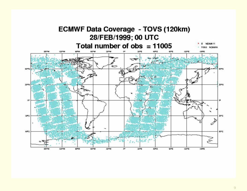
For a time window of ±3 hours, there are typically 10 to100 thousand observations of the atmosphere, two orders ofmagnitude less than the number of degrees of freedom ofthe model.
12

Insu!ciency of Data CoverageModern primitive equations models have a number ofdegrees of freedom of the order of 107.
For a time window of ±3 hours, there are typically 10 to100 thousand observations of the atmosphere, two orders ofmagnitude less than the number of degrees of freedom ofthe model.
Moreover, they are distributed nonuniformly in space andtime.
It is necessary to use additional information, called thebackground field, first guess or prior information.
A short-range forecast is used as the first guess in opera-tional data assimilation systems.
Present-day operational systems typically use a 6-h cycleperformed four times a day.
12
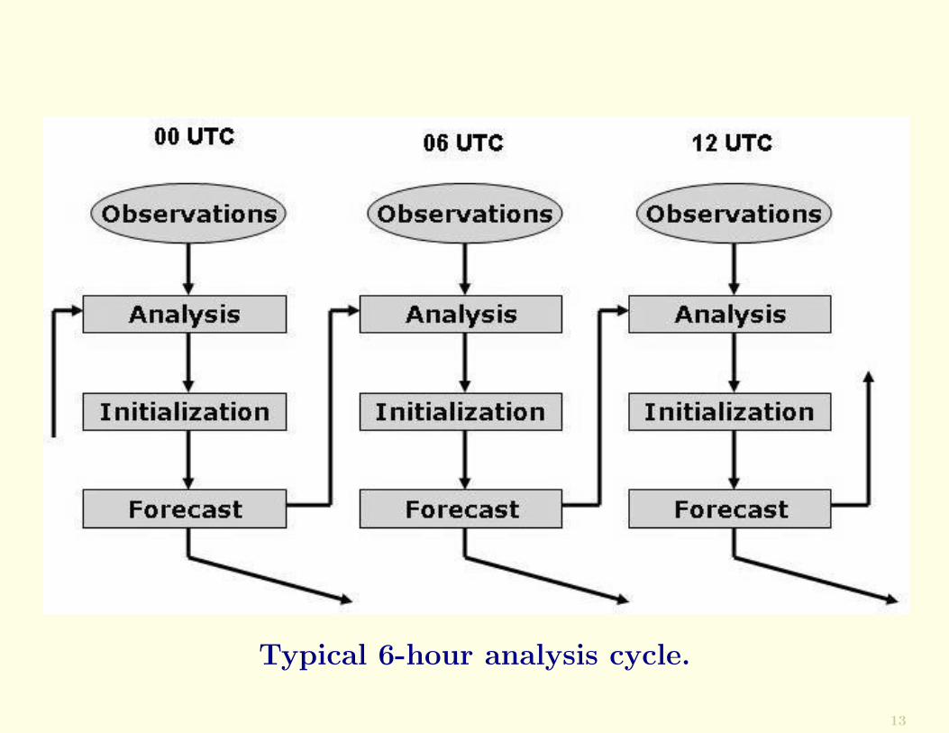
Typical 6-hour analysis cycle.
13
Suppose the background field is a model 6-h forecast:
xb
14
Suppose the background field is a model 6-h forecast:
xb
To obtain the background or first guess “observations”, themodel forecast is interpolated to the observation location
14
Suppose the background field is a model 6-h forecast:
xb
To obtain the background or first guess “observations”, themodel forecast is interpolated to the observation location
If the observed quantities are not the same as the modelvariables, the model variables are converted to observedvariables yo.
The first guess of the observations is denoted
H(xb)
where H is called the observation operator.
The di!erence between the observations and the background,
yo !H(xb) ,
is called the observational increment or innovation.
14

The analysis xa is obtained by adding the innovations to thebackground field with weights W that are determined basedon the estimated statistical error covariances of the forecastand the observations:
xa = xb + W[yo !H(xb)]
15

The analysis xa is obtained by adding the innovations to thebackground field with weights W that are determined basedon the estimated statistical error covariances of the forecastand the observations:
xa = xb + W[yo !H(xb)]
Di!erent analysis schemes (SCM, OI, 3D-Var, and KF) arebased on this equation, but di!er by the approach taken tocombine the background and the observations to producethe analysis.
Earlier methods such as the SCM used weights which weredetermined empirically.
The weights were a function of the distance between the ob-servation and the grid point, and the analysis wass iteratedseveral times.
15

In Optimal Interpolation (OI), the matrix of weights W isdetermined from the minimization of the analysis errors ateach grid point.
16

In Optimal Interpolation (OI), the matrix of weights W isdetermined from the minimization of the analysis errors ateach grid point.
In the 3D-Var approach one defines a cost function propor-tional to the square of the distance between the analysisand both the background and the observations.
This cost function is minimized to obtain the analysis.
Lorenc (1986) showed that OI and the 3D-Var approach areequivalent if the cost function is defined as:
J =1
2
![yo !H(x)]TR!1[yo !H(x)] + (x! xb)
TB!1(x! xb)"
The cost function J measures:
• The distance of a field x to the observations (first term)
• The distance to the background xb (second term).
16
The distances are scaled by the observation error covarianceR and by the background error covariance B respectively.
The minimum of the cost function is obtained for x = xa,which is defined as the analysis.
17

The distances are scaled by the observation error covarianceR and by the background error covariance B respectively.
The minimum of the cost function is obtained for x = xa,which is defined as the analysis.
The analysis obtained by OI and 3DVar is the same if theweight matrix is given by
W = BHT (HBHT + R!1)!1
The di!erence between OI and the 3D-Var approach is inthe method of solution:
• In OI, the weights W are obtained for each grid point orgrid volume, using suitable simplifications.
• In 3D-Var, the minimization of J is performed directly, al-lowing for additional flexibility and a simultaneous globaluse of the data.
17
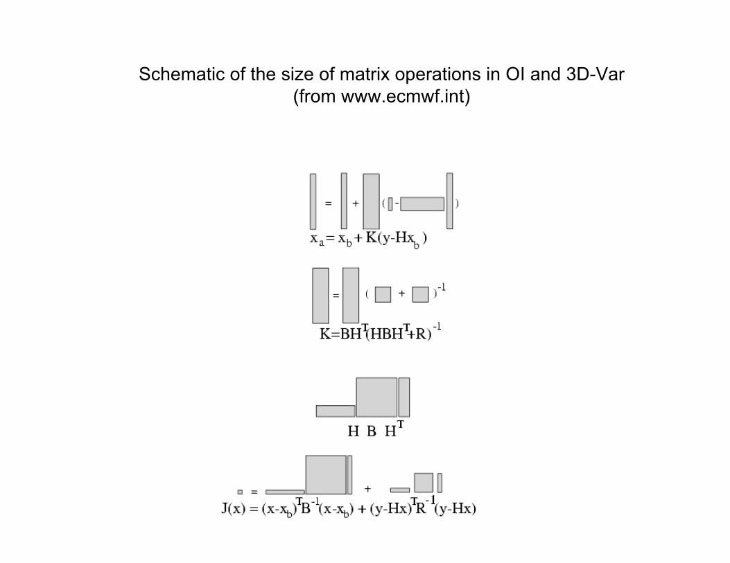
Schematic of the size of matrix operations in OI and 3D-Var
(from www.ecmwf.int)

Recently, the variational approach has been extended tofour dimensions, by including within the cost function thedistance to observations over a time interval (assimilationwindow).
18

Recently, the variational approach has been extended tofour dimensions, by including within the cost function thedistance to observations over a time interval (assimilationwindow).
This is called four-dimensional variational assimilation (4DVar).
18

Recently, the variational approach has been extended tofour dimensions, by including within the cost function thedistance to observations over a time interval (assimilationwindow).
This is called four-dimensional variational assimilation (4DVar).
In the analysis cycle, the importance of the model cannotbe overemphasized:
18
Recently, the variational approach has been extended tofour dimensions, by including within the cost function thedistance to observations over a time interval (assimilationwindow).
This is called four-dimensional variational assimilation (4DVar).
In the analysis cycle, the importance of the model cannotbe overemphasized:
• It transports information from data-rich to data-poorregions
18

Recently, the variational approach has been extended tofour dimensions, by including within the cost function thedistance to observations over a time interval (assimilationwindow).
This is called four-dimensional variational assimilation (4DVar).
In the analysis cycle, the importance of the model cannotbe overemphasized:
• It transports information from data-rich to data-poorregions
• It provides a complete estimation of the four-dimensionalstate of the atmosphere.
18
Recently, the variational approach has been extended tofour dimensions, by including within the cost function thedistance to observations over a time interval (assimilationwindow).
This is called four-dimensional variational assimilation (4DVar).
In the analysis cycle, the importance of the model cannotbe overemphasized:
• It transports information from data-rich to data-poorregions
• It provides a complete estimation of the four-dimensionalstate of the atmosphere.
The introduction of 4DVar at ECMWF has resulted in markedimprovements in the quality of medium-range forecasts.
End of Introduction
18

21

Background FieldFor operational models, it is not enough to perform spatialinterpolation of observations into regular grids:
There are not enough data available to define the initialstate.
23

Background FieldFor operational models, it is not enough to perform spatialinterpolation of observations into regular grids:
There are not enough data available to define the initialstate.
The number of degrees of freedom in a modern NWP modelis of the order of 107.
The total number of conventional observations is of the or-der of 104–105.
There are many new types of data, such as satellite andradar observations, but:
• they don’t measure the variables used in the models
• their distribution in space and time is very nonuniform.
23

Background FieldIn addition to observations, it is necessary to use a firstguess estimate of the state of the atmosphere at the gridpoints.
24

Background FieldIn addition to observations, it is necessary to use a firstguess estimate of the state of the atmosphere at the gridpoints.
The first guess (also known as background field or priorinformation) is our best estimate of the state of the atmo-sphere prior to the use of the observations.
A short-range forecast is normally used as a first guess inoperational systems in what is called an analysis cycle.
24
Background FieldIn addition to observations, it is necessary to use a firstguess estimate of the state of the atmosphere at the gridpoints.
The first guess (also known as background field or priorinformation) is our best estimate of the state of the atmo-sphere prior to the use of the observations.
A short-range forecast is normally used as a first guess inoperational systems in what is called an analysis cycle.
If a forecast is unavailable (e.g., if the cycle is broken), wemay have to use climatological fields . . .
. . . but they are normally a poor estimate of the initial state.
24

Global 6-h analysis cycle (00, 06, 12, and 18 UTC).25

Regional analysis cycle, performed (perhaps) every hour.26

Intermittent data assimilation is used in most global oper-ational systems, typically with a 6-h cycle performed fourtimes a day.
27
Intermittent data assimilation is used in most global oper-ational systems, typically with a 6-h cycle performed fourtimes a day.
The model forecast plays a very important role:
27
Intermittent data assimilation is used in most global oper-ational systems, typically with a 6-h cycle performed fourtimes a day.
The model forecast plays a very important role:
• Over data-rich regions, the analysis is dominated by theinformation contained in the observations.
27
Intermittent data assimilation is used in most global oper-ational systems, typically with a 6-h cycle performed fourtimes a day.
The model forecast plays a very important role:
• Over data-rich regions, the analysis is dominated by theinformation contained in the observations.
• In data-poor regions, the forecast benefits from the infor-mation upstream.
For example, 6-h forecasts over the North Atlantic Oceanare relatively good, because of the information coming fromNorth America.
27

Intermittent data assimilation is used in most global oper-ational systems, typically with a 6-h cycle performed fourtimes a day.
The model forecast plays a very important role:
• Over data-rich regions, the analysis is dominated by theinformation contained in the observations.
• In data-poor regions, the forecast benefits from the infor-mation upstream.
For example, 6-h forecasts over the North Atlantic Oceanare relatively good, because of the information coming fromNorth America.
The model is able to transport information from data-richto data-poor areas.
27
Least Squares Method (Kalnay, 5.3)We start with a toy model example, the two temperaturesproblem.

Least Squares Method (Kalnay, 5.3)We start with a toy model example, the two temperaturesproblem.
We use two methods to solve it, a sequential and a vari-ational approach, and find that they are equivalent: theyyield identical results.
Least Squares Method (Kalnay, 5.3)We start with a toy model example, the two temperaturesproblem.
We use two methods to solve it, a sequential and a vari-ational approach, and find that they are equivalent: theyyield identical results.
The problem is important because the methodology andresults carry over to multivariate OI, Kalman filtering, and3D-Var and 4D-Var assimilation.
If you fully understand the toy model, you should find themore realistic application straightforward.

Statistical estimationIntroduction. Each of you: Guess the temperature inthis room right now. How can we get a best estimate of thetemperature?
! ! !
2
Statistical estimationIntroduction. Each of you: Guess the temperature inthis room right now. How can we get a best estimate of thetemperature?
! ! !
The best estimate of the state of the atmosphere is obtainedby combining prior information about the atmosphere (back-ground or first guess) with observations.
In order to combine them optimally, we also need statisticalinformation about the errors in these pieces of information.
2

Statistical estimationIntroduction. Each of you: Guess the temperature inthis room right now. How can we get a best estimate of thetemperature?
! ! !
The best estimate of the state of the atmosphere is obtainedby combining prior information about the atmosphere (back-ground or first guess) with observations.
In order to combine them optimally, we also need statisticalinformation about the errors in these pieces of information.
As an introduction to statistical estimation, we consider thesimple problem, that we call the two temperatures problem:
2
Statistical estimationIntroduction. Each of you: Guess the temperature inthis room right now. How can we get a best estimate of thetemperature?
! ! !
The best estimate of the state of the atmosphere is obtainedby combining prior information about the atmosphere (back-ground or first guess) with observations.
In order to combine them optimally, we also need statisticalinformation about the errors in these pieces of information.
As an introduction to statistical estimation, we consider thesimple problem, that we call the two temperatures problem:
Given two independent observations T1 and T2, determinethe best estimate of the true temperature Tt.
2

Simple (toy) ExampleLet the two observations of temperature be
T1 = Tt + "1
T2 = Tt + "2
!
[For example, we might have two i!y thermometers].
3

Simple (toy) ExampleLet the two observations of temperature be
T1 = Tt + "1
T2 = Tt + "2
!
[For example, we might have two i!y thermometers].
The observations have errors "i, which we don’t know.
3

Simple (toy) ExampleLet the two observations of temperature be
T1 = Tt + "1
T2 = Tt + "2
!
[For example, we might have two i!y thermometers].
The observations have errors "i, which we don’t know.
Let E( ) represent the expected value, i.e., the average ofmany similar measurements.
3

Simple (toy) ExampleLet the two observations of temperature be
T1 = Tt + "1
T2 = Tt + "2
!
[For example, we might have two i!y thermometers].
The observations have errors "i, which we don’t know.
Let E( ) represent the expected value, i.e., the average ofmany similar measurements.
We assume that the measurements T1 and T2 are unbiased:
E(T1 ! Tt) = 0 , E(T2 ! Tt) = 0
or equivalently,E("1) = E("2) = 0
3

We also assume that we know the variances of the observa-tional errors:
E""21#
= #21 E
""22#
= #22
4

We also assume that we know the variances of the observa-tional errors:
E""21#
= #21 E
""22#
= #22
We next assume that the errors of the two measurementsare uncorrelated:
E("1"2) = 0
4
We also assume that we know the variances of the observa-tional errors:
E""21#
= #21 E
""22#
= #22
We next assume that the errors of the two measurementsare uncorrelated:
E("1"2) = 0
This implies, for example, that there is no systematic ten-dency for one thermometer to read high ("2 > 0) when theother is high ("2 > 0).
! ! !
4

We also assume that we know the variances of the observa-tional errors:
E""21#
= #21 E
""22#
= #22
We next assume that the errors of the two measurementsare uncorrelated:
E("1"2) = 0
This implies, for example, that there is no systematic ten-dency for one thermometer to read high ("2 > 0) when theother is high ("2 > 0).
! ! !
The above equations represent the statistical informationthat we need about the actual observations.
4
We estimate Tt as a linear combination of the observations:
Ta = a1T1 + a2T2
5
We estimate Tt as a linear combination of the observations:
Ta = a1T1 + a2T2
The analysis Ta should be unbiased:
E(Ta) = E(Tt)
5

We estimate Tt as a linear combination of the observations:
Ta = a1T1 + a2T2
The analysis Ta should be unbiased:
E(Ta) = E(Tt)
This impliesa1 + a2 = 1
5

We estimate Tt as a linear combination of the observations:
Ta = a1T1 + a2T2
The analysis Ta should be unbiased:
E(Ta) = E(Tt)
This impliesa1 + a2 = 1
Ta will be the best estimate of Tt if the coe!cients are chosento minimize the mean squared error of Ta:
#2a = E[(Ta ! Tt)
2] = E$%
a1(T1 ! Tt) + a2(T2 ! Tt)&2'
subject to the constraint a1 + a2 = 1.
This may be written
#2a = E[(a1"1 + a2"2)
2]
5

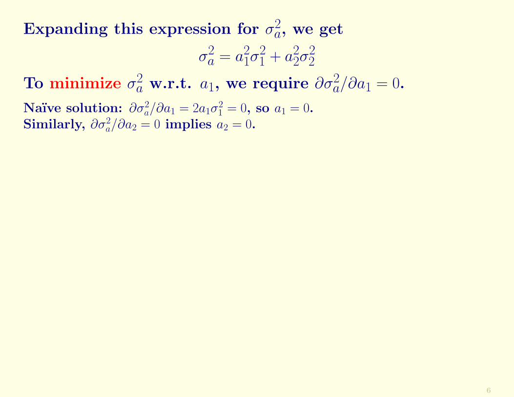
Expanding this expression for #2a, we get
#2a = a2
1#21 + a2
2#22
To minimize #2a w.r.t. a1, we require $#2
a/$a1 = 0.
6
Expanding this expression for #2a, we get
#2a = a2
1#21 + a2
2#22
To minimize #2a w.r.t. a1, we require $#2
a/$a1 = 0.
Naıve solution: $#2a/$a1 = 2a1#2
1 = 0, so a1 = 0.Similarly, $#2
a/$a2 = 0 implies a2 = 0.
6
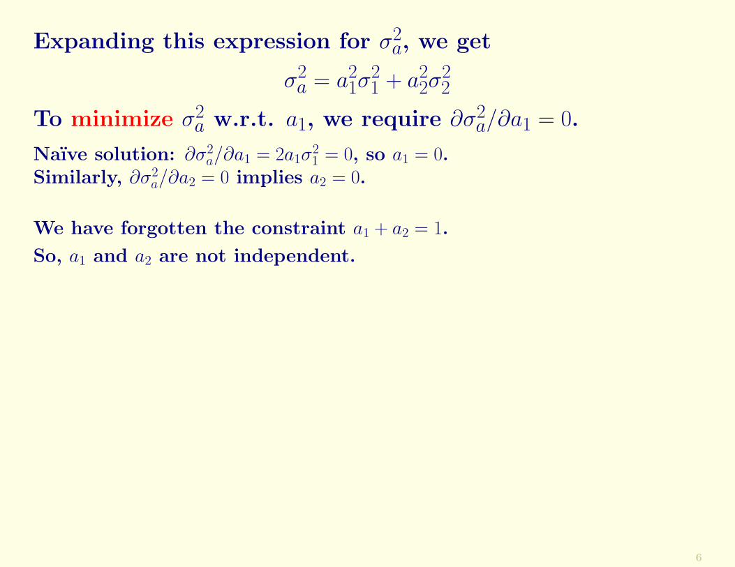
Expanding this expression for #2a, we get
#2a = a2
1#21 + a2
2#22
To minimize #2a w.r.t. a1, we require $#2
a/$a1 = 0.
Naıve solution: $#2a/$a1 = 2a1#2
1 = 0, so a1 = 0.Similarly, $#2
a/$a2 = 0 implies a2 = 0.
We have forgotten the constraint a1 + a2 = 1.
So, a1 and a2 are not independent.
6

Expanding this expression for #2a, we get
#2a = a2
1#21 + a2
2#22
To minimize #2a w.r.t. a1, we require $#2
a/$a1 = 0.
Naıve solution: $#2a/$a1 = 2a1#2
1 = 0, so a1 = 0.Similarly, $#2
a/$a2 = 0 implies a2 = 0.
We have forgotten the constraint a1 + a2 = 1.
So, a1 and a2 are not independent.
Substituting a2 = 1! a1, we get
#2a = a2
1#21 + (1! a1)
2#22
Equating the derivative w.r.t. a1 to zero, $#2a/$a1 = 0, gives
a1 =#2
2
#21 + #2
2
a2 =#2
1
#21 + #2
2
Thus, we have expressions for the weights a1 and a2 in termsof the variances (which are assumed to be known).
6

We define the precision to be the inverse of the variance. Itis a measure of the accuracy of the observations.
7

We define the precision to be the inverse of the variance. Itis a measure of the accuracy of the observations.
Note: The term precision, while a good one, does not haveuniversal currency, so it should be defined when used.
! ! !
7

We define the precision to be the inverse of the variance. Itis a measure of the accuracy of the observations.
Note: The term precision, while a good one, does not haveuniversal currency, so it should be defined when used.
! ! !
Substituting the coe!cients in #2a = a2
1#21 + a2
2#22, we obtain
#2a =
#21#
22
#21 + #2
2
This can be written in the alternative form:1
#2a
=1
#12 +
1
#22
Thus, if the coe"cients are optimal, the precision of theanalysis is the sum of the precisions of the measurements.
7

Variational approachWe can also obtain the same best estimate of Tt by mini-mizing a cost function.
8

Variational approachWe can also obtain the same best estimate of Tt by mini-mizing a cost function.
The cost function is defined as the sum of the squares of thedistances of T to the two observations, weighted by theirobservational error precisions:
J(T ) =1
2
((T ! T1)
2
#21
+(T ! T2)
2
#22
)
8

Variational approachWe can also obtain the same best estimate of Tt by mini-mizing a cost function.
The cost function is defined as the sum of the squares of thedistances of T to the two observations, weighted by theirobservational error precisions:
J(T ) =1
2
((T ! T1)
2
#21
+(T ! T2)
2
#22
)
The minimum of the cost function J is obtained is obtainedby requiring $J/$T = 0.
! ! !
Exercise: Prove that $J/$T = 0 gives the same value forTa as the least squares method.
8
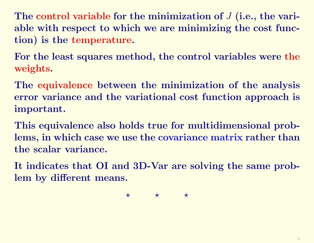
The control variable for the minimization of J (i.e., the vari-able with respect to which we are minimizing the cost func-tion) is the temperature.
For the least squares method, the control variables were theweights.
9
The control variable for the minimization of J (i.e., the vari-able with respect to which we are minimizing the cost func-tion) is the temperature.
For the least squares method, the control variables were theweights.
The equivalence between the minimization of the analysiserror variance and the variational cost function approach isimportant.
This equivalence also holds true for multidimensional prob-lems, in which case we use the covariance matrix rather thanthe scalar variance.
It indicates that OI and 3D-Var are solving the same prob-lem by di"erent means.
! ! !
9

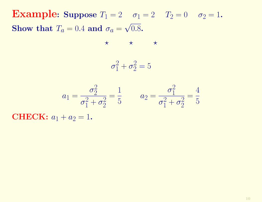
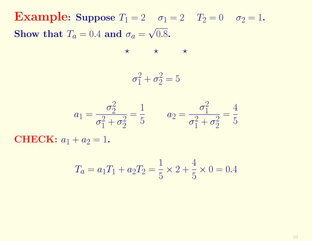
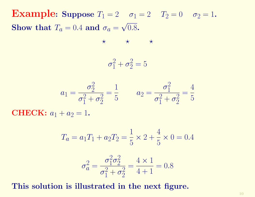
Example: Suppose T1 = 2 #1 = 2 T2 = 0 #2 = 1.
10

Example: Suppose T1 = 2 #1 = 2 T2 = 0 #2 = 1.
Show that Ta = 0.4 and #a ="
0.8.
! ! !
10

Example: Suppose T1 = 2 #1 = 2 T2 = 0 #2 = 1.
Show that Ta = 0.4 and #a ="
0.8.
! ! !
#21 + #2
2 = 5
10

Example: Suppose T1 = 2 #1 = 2 T2 = 0 #2 = 1.
Show that Ta = 0.4 and #a ="
0.8.
! ! !
#21 + #2
2 = 5
a1 =#2
2
#21 + #2
2
=1
5a2 =
#21
#21 + #2
2
=4
5
10
Example: Suppose T1 = 2 #1 = 2 T2 = 0 #2 = 1.
Show that Ta = 0.4 and #a ="
0.8.
! ! !
#21 + #2
2 = 5
a1 =#2
2
#21 + #2
2
=1
5a2 =
#21
#21 + #2
2
=4
5
CHECK: a1 + a2 = 1.
10
Example: Suppose T1 = 2 #1 = 2 T2 = 0 #2 = 1.
Show that Ta = 0.4 and #a ="
0.8.
! ! !
#21 + #2
2 = 5
a1 =#2
2
#21 + #2
2
=1
5a2 =
#21
#21 + #2
2
=4
5
CHECK: a1 + a2 = 1.
Ta = a1T1 + a2T2 =1
5# 2 +
4
5# 0 = 0.4
10

Example: Suppose T1 = 2 #1 = 2 T2 = 0 #2 = 1.
Show that Ta = 0.4 and #a ="
0.8.
! ! !
#21 + #2
2 = 5
a1 =#2
2
#21 + #2
2
=1
5a2 =
#21
#21 + #2
2
=4
5
CHECK: a1 + a2 = 1.
Ta = a1T1 + a2T2 =1
5# 2 +
4
5# 0 = 0.4
#2a =
#21#
22
#21 + #2
2
=4# 1
4 + 1= 0.8
10
Example: Suppose T1 = 2 #1 = 2 T2 = 0 #2 = 1.
Show that Ta = 0.4 and #a ="
0.8.
! ! !
#21 + #2
2 = 5
a1 =#2
2
#21 + #2
2
=1
5a2 =
#21
#21 + #2
2
=4
5
CHECK: a1 + a2 = 1.
Ta = a1T1 + a2T2 =1
5# 2 +
4
5# 0 = 0.4
#2a =
#21#
22
#21 + #2
2
=4# 1
4 + 1= 0.8
This solution is illustrated in the next figure.10

The probability distribution for a simple case.The analysis has a pdf with a maximum closer to T 2, and a smaller standard deviation than either observation.
11

Conclusion of the foregoing.
12
Simple Sequential AssimilationWe consider the ‘toy’ example as a prototype of afull multivariate OI.
13
Simple Sequential AssimilationWe consider the ‘toy’ example as a prototype of afull multivariate OI.
Recall that we wrote the analysis as a linear combination
Ta = a1T1 + a2T2
13
Simple Sequential AssimilationWe consider the ‘toy’ example as a prototype of afull multivariate OI.
Recall that we wrote the analysis as a linear combination
Ta = a1T1 + a2T2
The requirement that the analysis be unbiassed led toa1 + a2 = 1, so
Ta = T1 + a2(T2 ! T1)
13

Simple Sequential AssimilationWe consider the ‘toy’ example as a prototype of afull multivariate OI.
Recall that we wrote the analysis as a linear combination
Ta = a1T1 + a2T2
The requirement that the analysis be unbiassed led toa1 + a2 = 1, so
Ta = T1 + a2(T2 ! T1)
Assume that one of the two temperatures, say T1 = Tb, is notan observation, but a background value, such as a forecast.
Assume that the other value is an observation, T2 = To.
We can write the analysis as
Ta = Tb + W (To ! Tb)
where W = a2 can be expressed in terms of the variances.13

The least squares method gave us the optimal weight:
W =#2
b
#2b + #2
o
14

The least squares method gave us the optimal weight:
W =#2
b
#2b + #2
o
When the analysis is written as
Ta = Tb + W (To ! Tb)
the quantity (To!Tb) is called the observational innovation,i.e., the new information brought by the observation.
14

The least squares method gave us the optimal weight:
W =#2
b
#2b + #2
o
When the analysis is written as
Ta = Tb + W (To ! Tb)
the quantity (To!Tb) is called the observational innovation,i.e., the new information brought by the observation.
It is also known as the observational increment (with respectto the background).
14

The analysis error variance is, as before, given by
1
#2a
=1
#2b
+1
#2o
or #2a =
#2b#
2o
#2b + #2
o
15

The analysis error variance is, as before, given by
1
#2a
=1
#2b
+1
#2o
or #2a =
#2b#
2o
#2b + #2
o
The analysis variance can be written as
#2a = (1!W )#2
b
! ! !
15

The analysis error variance is, as before, given by
1
#2a
=1
#2b
+1
#2o
or #2a =
#2b#
2o
#2b + #2
o
The analysis variance can be written as
#2a = (1!W )#2
b
! ! !
Exercise: Verify all the foregoing formulæ.
! ! !
15

The analysis error variance is, as before, given by
1
#2a
=1
#2b
+1
#2o
or #2a =
#2b#
2o
#2b + #2
o
The analysis variance can be written as
#2a = (1!W )#2
b
! ! !
Exercise: Verify all the foregoing formulæ.
! ! !
We have shown that the simple two-temperatures problemserves as a paradigm for the problem of objective analysisof the atmospheric state.
15

Collection of Main EquationsWe gather the principal equations here:
16
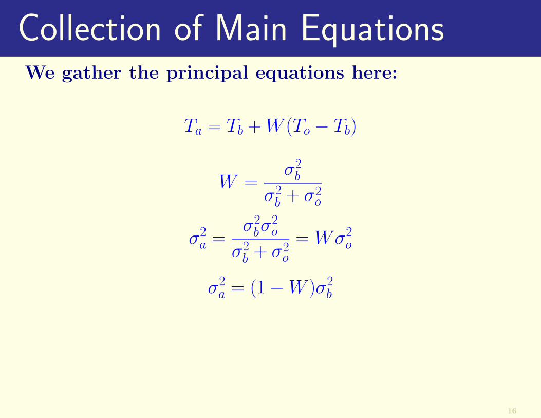
Collection of Main EquationsWe gather the principal equations here:
Ta = Tb + W (To ! Tb)
W =#2
b
#2b + #2
o
#2a =
#2b#
2o
#2b + #2
o
= W#2o
#2a = (1!W )#2
b
16

These four equations have been derived for the simplestscalar case . . .
. . . but they are important for the problem of data assim-ilation because they have exactly the same form as moregeneral equations:
17
These four equations have been derived for the simplestscalar case . . .
. . . but they are important for the problem of data assim-ilation because they have exactly the same form as moregeneral equations:
The least squares sequential estimation method is used forreal multidimensional problems (OI, interpolation, 3D-Varand even Kalman filtering).
17

These four equations have been derived for the simplestscalar case . . .
. . . but they are important for the problem of data assim-ilation because they have exactly the same form as moregeneral equations:
The least squares sequential estimation method is used forreal multidimensional problems (OI, interpolation, 3D-Varand even Kalman filtering).
Therefore we will interpret these four equations in detail.
17

The first equation
Ta = Tb + W (To ! Tb)
18

The first equation
Ta = Tb + W (To ! Tb)
This says:
The analysis is obtained by adding to the backgroundvalue, or first guess, the innovation (the di"erencebetween the observation and first guess), weightedby the optimal weight.
18

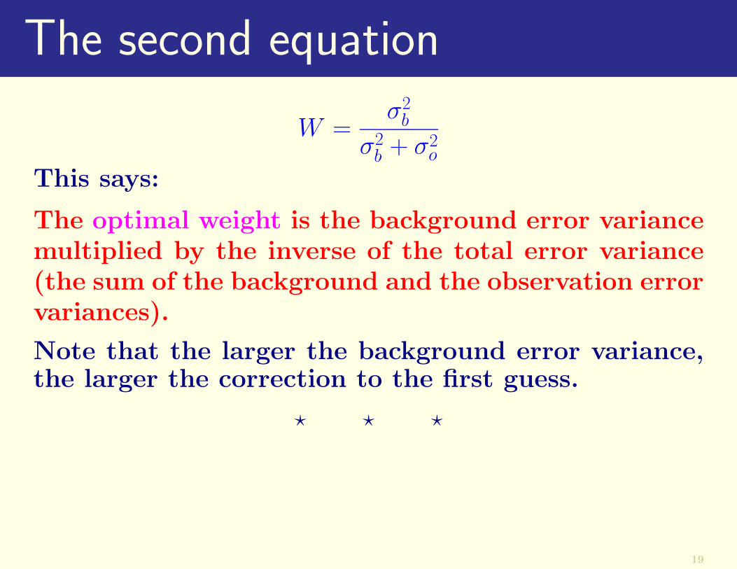
The second equation
W =#2
b
#2b + #2
o
This says:
The optimal weight is the background error variancemultiplied by the inverse of the total error variance(the sum of the background and the observation errorvariances).
19
The second equation
W =#2
b
#2b + #2
o
This says:
The optimal weight is the background error variancemultiplied by the inverse of the total error variance(the sum of the background and the observation errorvariances).
Note that the larger the background error variance,the larger the correction to the first guess.
! ! !
19

The second equation
W =#2
b
#2b + #2
o
This says:
The optimal weight is the background error variancemultiplied by the inverse of the total error variance(the sum of the background and the observation errorvariances).
Note that the larger the background error variance,the larger the correction to the first guess.
! ! !
Look at the limits: #2o = 0 ; #2
b = 0.
19

The third equationThe variance of the analysis is
#2a =
#2b#
2o
#2b + #2
o
20

The third equationThe variance of the analysis is
#2a =
#2b#
2o
#2b + #2
o
This can also be written1
#2a
=1
#2b
+1
#2o
20

The third equationThe variance of the analysis is
#2a =
#2b#
2o
#2b + #2
o
This can also be written1
#2a
=1
#2b
+1
#2o
This says:
The precision of the analysis (inverse of the analysiserror variance) is the sum of the precisions of thebackground and the observation.
20

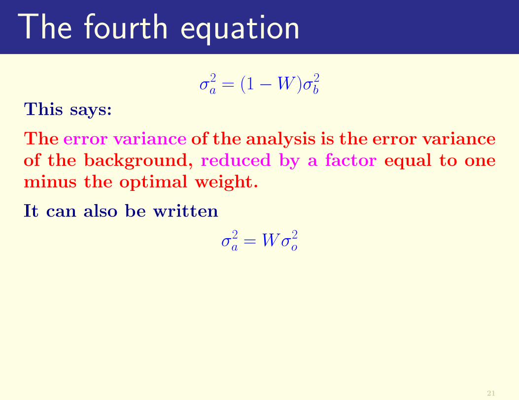
The fourth equation
#2a = (1!W )#2
b
This says:
The error variance of the analysis is the error varianceof the background, reduced by a factor equal to oneminus the optimal weight.
21
The fourth equation
#2a = (1!W )#2
b
This says:
The error variance of the analysis is the error varianceof the background, reduced by a factor equal to oneminus the optimal weight.
It can also be written
#2a = W#2
o
21

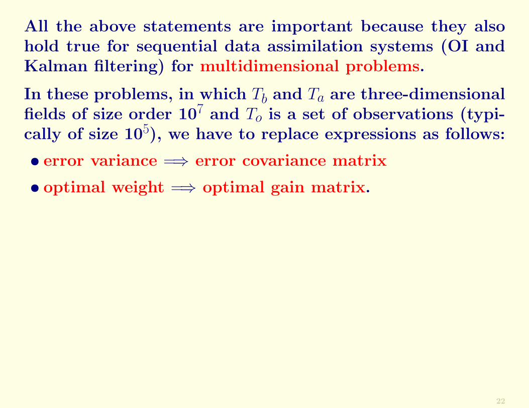
All the above statements are important because they alsohold true for sequential data assimilation systems (OI andKalman filtering) for multidimensional problems.
22

All the above statements are important because they alsohold true for sequential data assimilation systems (OI andKalman filtering) for multidimensional problems.
In these problems, in which Tb and Ta are three-dimensionalfields of size order 107 and To is a set of observations (typi-cally of size 105), we have to replace expressions as follows:
• error variance =$ error covariance matrix
22
All the above statements are important because they alsohold true for sequential data assimilation systems (OI andKalman filtering) for multidimensional problems.
In these problems, in which Tb and Ta are three-dimensionalfields of size order 107 and To is a set of observations (typi-cally of size 105), we have to replace expressions as follows:
• error variance =$ error covariance matrix
• optimal weight =$ optimal gain matrix.
22

All the above statements are important because they alsohold true for sequential data assimilation systems (OI andKalman filtering) for multidimensional problems.
In these problems, in which Tb and Ta are three-dimensionalfields of size order 107 and To is a set of observations (typi-cally of size 105), we have to replace expressions as follows:
• error variance =$ error covariance matrix
• optimal weight =$ optimal gain matrix.
Note that there is one essential tuning parameter in OI:
It is the ratio of the observationalvariance to the backgrounderror variance: *
#o
#b
+2
22
Application to AnalysisIf the background is a forecast, we can use the four equationsto create a simple sequential analysis cycle.
The observation is used once at the time it appears and thendiscarded.
23

Application to AnalysisIf the background is a forecast, we can use the four equationsto create a simple sequential analysis cycle.
The observation is used once at the time it appears and thendiscarded.
Assume that we have completed the analysis at time ti (e.g.,at 06 UTC), and we want to proceed to the next cycle (timeti+1, or 12 UTC).
The analysis cycle has two phases, a forecast phase to up-date the background Tb and its error variance #2
b, and ananalysis phase, to update the analysis Ta and its error vari-ance #2
a.
23

Typical 6-hour analysis cycle.
24

Forecast PhaseIn the forecast phase of the analysis cycle, the backgroundis first obtained through a forecast:
Tb(ti+1) = M [Ta(ti)]
where M represents the forecast model.
25
Forecast PhaseIn the forecast phase of the analysis cycle, the backgroundis first obtained through a forecast:
Tb(ti+1) = M [Ta(ti)]
where M represents the forecast model.
We also need the error variance of the background.
25

Forecast PhaseIn the forecast phase of the analysis cycle, the backgroundis first obtained through a forecast:
Tb(ti+1) = M [Ta(ti)]
where M represents the forecast model.
We also need the error variance of the background.
In OI, this is obtained by making a suitable simple assump-tion, such as that the model integration increases the ini-tial error variance by a fixed amount, a factor a somewhatgreater than 1:
#2b(ti+1) = a#2
a(ti)
This allows the new weight W (ti+1) to be estimated using
W =#2
b
#2b + #2
o
25

Analysis PhaseIn the analysis phase of the cycle we get the new observationTo(ti+1), and we derive the new analysis Ta(ti+1) using
Ta = Tb + W (To ! Tb)
26

Analysis PhaseIn the analysis phase of the cycle we get the new observationTo(ti+1), and we derive the new analysis Ta(ti+1) using
Ta = Tb + W (To ! Tb)
The estimates of #2b is from
#2b(ti+1) = a#2
a(ti)
26

Analysis PhaseIn the analysis phase of the cycle we get the new observationTo(ti+1), and we derive the new analysis Ta(ti+1) using
Ta = Tb + W (To ! Tb)
The estimates of #2b is from
#2b(ti+1) = a#2
a(ti)
The new analysis error variance #2a(ti+1) comes from
#2a = (1!W )#2
b
It is smaller than the background error.
After the analysis, the cycle for time ti+1 is completed, andwe can proceed to the next cycle.
26

Reading Assignment
Study the Remarks in Kalnay, §5.3.1
27