Motorcycle Dynamometer

Philip Harrison

B.A. (Mod.) in Computer Science

Final Year Project 2004

Supervisor: Mr. Michael Manzke

2

Declaration

I hereby declare that this thesis is entirely my own work and that it has not been

submitted as an exercise for a degree at any other university.

__________________________ 15th April 2004

3

Acknowledgments IVO GmbH & Co. KG (http://www.ivo.de)

Supply of the CANOpen enabled multi-turn encoder used for RPM detection

Softing AG (http://www.softing.com/en)

Supply of the CANOpen protocol stack and API for use with the Softing CAN

interface card

Trinity College Distributed Systems Group

Supply of the Softing CAN interface card

Halligans Truck Breakers

Supply of the truck brake drums

Philips Electronics

Supply of microcontroller, CAN Controller and CAN transceiver chips

4

Abstract

The purpose of this report is to document the design and implementation of a

motorcycle dynamometer. Dynamometers are typically used by mechanics and tuners

to evaluate the change in power output of an engine before and after a modification is

made to that engine. The report details the physical mechanics needed to test the

engine, the data acquisition mechanisms and the software written to process and

display the data. The outcome of the project was successful.

5

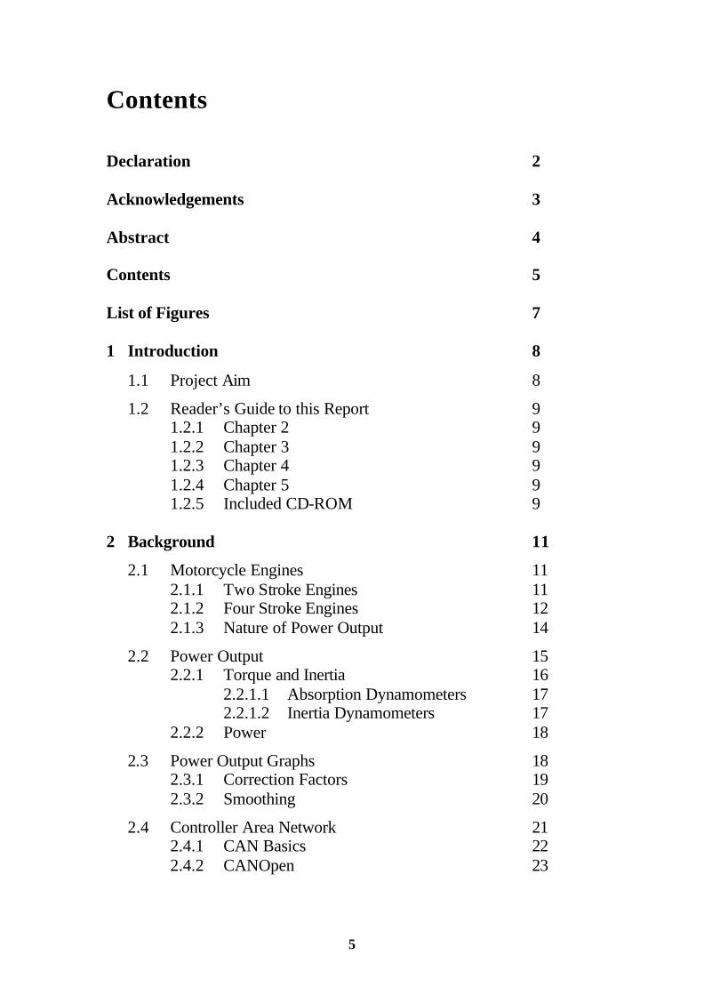
Contents Declaration 2 Acknowledgements 3 Abstract 4 Contents 5 List of Figures 7 1 Introduction 8

1.1 Project Aim 8

1.2 Reader’s Guide to this Report 9 1.2.1 Chapter 2 9 1.2.2 Chapter 3 9 1.2.3 Chapter 4 9 1.2.4 Chapter 5 9 1.2.5 Included CD-ROM 9 2 Background 11

2.1 Motorcycle Engines 11 2.1.1 Two Stroke Engines 11 2.1.2 Four Stroke Engines 12 2.1.3 Nature of Power Output 14

2.2 Power Output 15 2.2.1 Torque and Inertia 16 2.2.1.1 Absorption Dynamometers 17 2.2.1.2 Inertia Dynamometers 17 2.2.2 Power 18

2.3 Power Output Graphs 18 2.3.1 Correction Factors 19 2.3.2 Smoothing 20

2.4 Controller Area Network 21 2.4.1 CAN Basics 22 2.4.2 CANOpen 23

6

3 Design 25

3.1 Overview 25

3.2 Mechanics 25

3.3 Data Acquisition 27

3.4 Sensing 29

3.5 Software 31 3.5.1 Acquiring the Data 31 3.5.2 Interpreting and Displaying the Data 32 4 Implementation 34

4.1 Overview 34

4.2 Mechanics 34

4.3 Data Acquisition 36

4.4 Sensing 37

4.5 Software 37 4.5.1 Acquiring the Data 37 4.5.2 Data Storage 38 4.5.3 Graphical User Interface 39 4.5.4 DynoSoft Usage 41 4.5.5 CANMan 41 5 Evaluation 43

5.1 Critique 43 5.1.1 Mechanics 43 5.1.2 Data Acquisition 43 5.1.3 Sensing 44 5.1.4 Software 44

5.2 Future Work 45

5.3 Summary 45

5.4 Conclusions 46

Bibliography 47

7

List of figures 1.1 A Commercial Motorcycle Dynamometer 8

2.1 A Basic Two Stroke Engine 12

2.2 A Basic Four Stroke Engine 13

2.3 Example Power Output Graph 14

2.4 Torque and Power Graph 19

2.5 Noisy Graph 21

2.6 Smoothened Graph 21

2.7 CAN Frame Format 22

2.8 CAN Network Layout 23

3.1 Basic Dynamometer Schematic 27

3.2 CAN Node 29

3.3 IVO Encoder 30

3.4 Honeywell HIH-3610 Humidity Sensor 31

4.1 Brake Drum and Half Axle 34

4.2 Drums Mounted to H Section 35

4.3 Finished Dynamometer Structure 36

4.4 Final Data Acquisition Layout 36

4.5 DynoSoft Screenshot 40

4.6 CANMan Screenshot 42

8

Chapter 1

Introduction 1.1 Project Aim

The aim of this project is to develop a tool to aid performance tuning of motorcycle

engines. The tool should allow the user test a motorcycle, modify the engine in some

way, run a second test then compare the two sets of results and hence evaluate the

effect the modification has on the power output of the engine. The user can then

decide to leave the modification to the engine intact if the result was satisfactory or try

something else if it was not. Measuring power output accurately outside of laboratory

conditions is difficult and impractical, so the main aim of this project is to develop a

tool that produces repeatable results.

Figure 1.1: A Commercial Motorcycle Dynamometer

9

1.2 Reader’s Guide to this Report

This section acts as a guide to the reader, describing the contents of each chapter of

this report.

1.2.1 Chapter 2

This chapter aims to explain enough about the concepts behind and the technologies

used in this project so the reader will understand chapters three and four. It also

attempts to put the project in context by explaining what it is the project is trying to

achieve and why.

1.2.2 Chapter 3

This chapter describes the design stage of the project, describing in detail what the

project aimed to achieve.

1.2.3 Chapter 4

This chapter describes the implementation of the project, discussing how the designs

covered in chapter three worked out and were finally implemented.

1.2.4 Chapter 5

This chapter aims to evaluate the project, discussing the successes of the project,

problems encountered during the project and possible future work to be carried out on

the project.

1.2.5 Included CD-ROM

The CD-ROM included with this report contains the Microsoft Power Point

presentation file used during the project demonstration, some digital photographs of

the dynamometer in JPEG format, a video of a dynamometer test done on a Kawasaki

KX125 in Microsoft’s AVI (Audio Video Interleave) format and the Microsoft Visual

C++ 6.0 project files of the software (DynoSoft and CANMan) written for this project,

including source code and the compiled executables. The executables were compiled

using Microsoft Visual C++ 6.0 running in Microsoft Windows XP but should work

10

on all Microsoft Windows versions after and including Windows 95. The software

uses the MFC (Microsoft Foundation Classes) so requires the MFC drivers be

installed, it also uses the Softing CANOpen API (Application Programming Interface)

so requires the CANOpen driver (canopen.dll) be present on the system, either in the

immediate program directory or in the Windows system directory. All images used in

this report are also on the CD in case they are unclear when printed.

11

Chapter 2

Background 2.1 Motorcycle Engines

The dynamometer built during this project was aimed at testing motocross engines,

which typically range in size from 50cc1 to 500cc with a power output of roughly

5HP2 to 60HP respectively. The two main types of engine used in motocross bikes

today are the two stroke spark ignition engine and the Otto four stroke spark ignition

engine. A brief description of the operation of two and four stroke engines will now

be given to put the project in context but I encourage the reader to look up the

references given for a more complete description.

2.1.1 Two Stroke Engines

The two stroke engine is by far the simpler of the two types of engines employed in

motocross bikes. The piston travelling upwards causes a vacuum to form behind it

which draws air into the engine through a carburettor where fuel (which has oil

premixed with it at a ratio of roughly 30 parts fuel to 1 part oil) is sprayed into the air

stream and carried along with it, partially atomised. The incoming charge enters

directly into the crankcase via a one-way valve where the surrounding heat causes the

fuel to evaporate, leaving its load of oil behind to lubricate the crank bearings and

cylinder wall. When the piston is descending the pressure created in the crankcase

will cause the one-way valve to close, the intake charge of air and fuel in the

crankcase will then begin to be compressed. The descend ing piston will first reveal

the exhaust port, then the transfer ports, allowing the compressed intake charge rush

up the ports into the combustion chamber. The intake charge entering the combustion

chamber also serves to scavenge 3 the exhaust gas from the previous combustion. The

1 cc – Cubic centimetres. 2 HP – Horsepower – Typically used to describe the amount of work done over time by a machine. 3 scavenge – The incoming charge of unburned air and fuel is used to force the burned exhaust gas out the exhaust port.

12

piston will reach bottom dead centre4 and start ascending again, compressing the

intake charge above it once it has blocked off the transfer ports and exhaust port.

Approximately 15º 5 before top dead centre6 the spark plug will fire, igniting the

compressed charge of air and fuel. The rapidly expanding flame front creates huge

pressure (800-1300psi [1]) above the piston which forces it down the cylinder. Most

125cc motocross engines will repeat this cycle over 13,000 times per minute at full

throttle. For more information on the operation of two stroke engines please see

reference [2] and Chapter 1 of reference [3] in the bibliography section.

Figure 2.1: A Basic Two Stroke Engine

2.1.2 Four Stroke Engines

Four stroke engines draw their air and fuel into the combustion chamber through ports

in the cylinder head, therefore the crank and cylinder must be lubricated by the oil in

the sump rather then premixed oil falling out of the intake charge as in a two stroke.

The cylinder head of a four stroke will typically have two intake and two exhaust

ports, the flow through which is controlled by valves. These valves are opened and

closed by a series of chains and cams driven directly off the crank, so a particular

valve always opens at the exact same place in the rotation of the crank. During

combustion all the valves will be closed off and will remain closed until the piston has

descended to bottom dead centre and is on its way back up the cylinder again. The

exhaust valves will then open allowing the ascending piston force the burned exhaust 4 bottom dead centre (BDC) – the point in a piston’s stroke where it is at its lowest point, closest to the crank 5 15º – current location in the stroke is typically stated in degrees of rotation of the crank 6 top dead centre (TDC) – the point in the piston’s stroke where it is at its highest point, furthest from the crank

13

gas out the exhaust ports and eventually out the exhaust. Once the piston reaches top

dead centre the exhaust valves will close and the intake valves will open, the vacuum

caused above the piston as it descends in the cylinder will pull air into the engine

through the carburettor, where fuel is added to the intake charge as before. As the

piston again reaches bottom dead centre the intake valves close and the piston then

ascends, compressing the unburned intake charge in front of it. Just before the piston

reaches top dead centre the spark plug fires, causing a flame front to advance from the

spark plug, this works in exactly the same way as in a two stroke engine. Therefore

the piston has to travel up the cylinder twice and down the cylinder twice to complete

a full cycle, hence the name four stroke, whereas the two stroke only need travel up

and down once to complete a full cycle. Theoretically this fact should allow two

strokes produce twice as much power as four strokes revving to the same point.

Unfortunately inefficiencies limit the two strokes somewhat. However 125cc two

stroke motocross bikes are generally raced with 250cc four stroke bikes, so the theory

is nearly accurate. For more information on the operation of four stroke engines

please see reference [4] and Chapter 1 of reference [5] in the bibliography section.

Figure 2.2: A Basic Four Stroke Engine

14

2.1.3 Nature of Power Output

For both types of engine there is a certain point, in terms of RPM7, at which

maximum power will be produced. This point is influenced by many factors in the

engine, but is basically the point in the RPM range at which everything in the engine

is timed perfectly; the perfect amount of air enters the combustion chamber, the

exhaust gas is fully expelled from the combustion chamber, the valves or ports closed

and the spark plug fired at the ideal time etc. Before and after this point the timing of

the various components of the engine becomes more out of synchronisation leading to

a drop off in power, hence the power output of the engine rises to a peak then

descends again. The power peak can be reshaped or moved up or down in the RPM

range by changing various engine components to alter the point at which the timing of

all the components comes together. A beginner racer will want this peak to be broad

and lower down in the RPM range as they won’t have the ability to keep the engine in

a tight high RPM range through corners and during acceleration. Whereas a

professional racer will keep the engine at high RPMs most of the time, using the

clutch and gearbox, so he/she will want a tight high peak further up in the RPM range.

Figure 2.3: Example Power Output Graph

Figure 2.3 shows a power output graph of a two stroke 125cc motocross engine, RPM

of the engine is on the x-axis and the power output (in horsepower) is on the y-axis.

7 RPM – Revolutions per minute – Refers to the number of times a rotating object completes one full turn in one minute. Often used as an adjective to describe the speed the crank of an engine is rotating.

15

The red curve shows the power output of the stock8 engine while the blue curve shows

the power output of the same engine, modified for a professional racer. The broad

power curve of the stock engine would make it suitable for a beginner to intermediate

racer, while a professional racer would find the power too spread out and low in the

RPM range, a tighter peak with maximum power output of 3-4HP greater then stock

and occurring at 11,500-12,000RPM would be more appropriate. A tuner trying to set

this bike up for a professional racer can use a dynamometer to generate a power

output graph such as red curve in Figure 2.3, make some changes to the engine to

attempt to shift the power up the RPM range then perform another test (such as the

blue curve in Figure 2.3) on the dynamometer to determine if the changes he made

were the correct ones, this cycle will be repeated until the tuner is satisfied with the

power output of the engine. Figure 2.3 shows before and after tests of engine tuning

done in this fashion. The tuner can immediately see from this graph the effects of the

changes he/she made to the engine and how successful they are.

2.2 Power Output

A motorcycle engine converts the reciprocating motion of the piston to circular

motion using a crank. The circular motion of the crank is transferred through the

clutch to the transmission, which in turn transfers it to the rear wheel using a chain

and sprockets connected at one end to the transmission and the other directly to the

wheel. The wheel then converts the circular motion to linear motion driving the

motorcycle forward. Gearing is used all the way from the crank to the rear wheel to

reduce the wheel’s angular velocity with respect to the crank’s angular velocity. For

example the 2000 Honda CR125 motocross bike in 5th gear has a total gearing

reduction from the crank to rear wheel of 14.23, meaning the crank will rotate 14.23

times to produce one full turn of the rear wheel. To measure the power output of the

engine one must measure the force produced by the rear wheel of the motorcycle, the

total gearing also has to be taken into account so the RPM of crank can be determined

and displayed on a graph. It is also possible to measure the power output produced

directly at the crank but this doesn’t give a true reflection of the power one would feel

riding the motorcycle. 8 Stock – Meaning the part in question is as it would come from the manufacturer, unmodified.

16

2.2.1 Torque and Inertia

Although it would be possible to measure and record the acceleration of a motorcycle

as it is ridden down a road and mathematically derive power output it would be

difficult to achieve repeatability with so many variables present, such as variable wind

resistance or differences in how the bike is accelerated from one test to the next, it

would also be impractical as speeds of over 60mph would be necessary. The

alternative is to fix the motorcycle in position and place the rear wheel on a form of

rolling road. However with the motorcycle lifted off the ground there is no load on

the engine, as there would be when it has to accelerate the mass of bike and rider

down a road, this will allow the engine accelerate much quicker and appear to make

considerably more power then it can under normal load. We are trying to measure the

power output of the engine by measuring the force applied to the ground by the rear

wheel. Isaac Newton’s Second Law of Motion states:

Force = Mass x Acceleration

The rotational equivalent of this law is:

Torque = Moment of Inertia x Angular Acceleration

Torque is the name given to a turning force or the force applied to a body to cause

angular acceleration of that body about an axis. Toque is generally expressed in foot-

pounds when being used in relation to engines. The torque being measured with a

dynamometer is the turning force applied to the drum of the rolling road by the rear

wheel of the motorcycle. However without a load on the rear wheel the mass or

moment of inertia is effectively 0, meaning there is no way of calculating this force9.

Therefore to measure the power output one must put a load on the engine to simulate

the load it experiences during normal operation. There are a few different methods of

providing this load, the two main methods employed in dynamometers are absorption

and inertia. For a comparison table of the different dynamometer types please see

reference [6] in the bibliography section.

9 The moment of inertia is not actually 0 because the clutch, transmission and other rotating engine components provide a mass and hence moment of inertia but this is ignored as measuring the parts would be difficult and the inertia provided by these parts is insignificant compared to the load provided by the dynamometer drum.

17

2.2.1.1 Absorption Dynamometers

Absorption provides a load using a brake to slow the acceleration of the rolling road,

the braking force applied must be varied depending on the current speed of the engine

and the actual braking force applied must be known so it can be taken into account in

the mathematics. Typical brakes used are; water brake absorbers, Eddy current

absorbers, friction brake, AC/DC motor-generators. The need to dynamically control

the braking force applied and accurately measure that force makes this method

difficult to develop.

2.2.1.2 Inertia Dynamometers

The definition of inertia, also known as the moment of inertia, is the measure of a

body's ability to resist angular acceleration about a specific axis. The greater the

moment of inertia of a body, the more torque it will take to change the angular

velocity of that body. [7] The inertia of a body can either be measured empirically

using the method described at reference [8] or calculated using this formula for a solid

cylindrical drum made of uniform material:

Inertia = (Mass / 2) x Radius²

Instead of using a rolling road as mentioned earlier, one can use a heavy drum that the

rear wheel of the motorcycle sits against and accelerates. Either method of

determining the inertia of the drum may be used, though if the drum is not solid

calculating the inertia becomes much more difficult leaving the empirical method as

preference. The inertial force of the drum now provides the load for the engine of the

motorcycle, so a drum of sufficient inertia must be chosen to roughly match the load

the engine normally experiences under standard operating conditions. The inertia of

the drum does not need to match this normal operating load exactly because the

formula for torque will take into account too light or heavy a drum, the only concern

is if the drum is considerably too light or heavy the engine will perform significantly

different to normal. Though it is important to remember that the main aim of this

dynamometer is to provide repeatable results, which it will achieve even with a very

light or heavy drum, the actual power figures may be slightly incorrect but this is of

little importance.

Knowing the inertia of the drum, the acceleration of that drum must be monitored as

the motorcycle accelerates it. Then using the given formula, torque can be calculated

18

for all the sample points taken of the drum’s acceleration. A graph showing time or

speed versus toque can then be plotted.

2.2.2 Power

Torque gives a metric to the force the rear wheel applies to the dynamometer drum

but it doesn’t show the amount of work being done by the engine. For instance an

engine producing 20ft- lbs of torque at 13,000RPM is doing more work then an engine

producing 20ft-lbs of torque at 6,000RPM. The amount of work done is known as

power and when used in relation to engines is typically expressed in either

horsepower or kilowatts. Power is often defined as the amount of work done over a

period of time but when describing the power of an engine, power is defined as the

work done at a particular engine speed. The formula for power is as follows:

Power = Torque x Angular Velocity

This formula yields power in kilowatts, which can be converted to horsepower by

multiplying by 1.34. Alternatively a simplified formula, allowing direct calculation of

power expressed in horsepower from an RPM figure, without first calculating angular

velocity is as follows:

Horsepower = (Torque x RPM) / 5252

A graph of engine RPM, calculated by multiplying the current drum RPM by the total

gearing factor from the drum to the crank, versus horsepower can now be plotted for

all the samples taken of the dynamometer drum RPM. For more information

concerning torque and power and their meanings with respect to motorcycle engines

please see reference [9] in the bibliography section.

2.3 Power Output Graphs

The calculation of torque and power gives rise to two different graphs, torque vs.

RPM and power vs. RPM. However both graphs are of interest to a motorcycle tuner

so both are often shown on power output graphs, with power on the left y-axis and

toque on an additional right y-axis. The two graphs will always be different shapes,

with the power peak occurring later then the torque peak in the RPM range. The RPM

range between the torque peak and the power peak is what is referred to as the power-

band of an engine, a racer wants to keep the revs of the engine in this power-band

19

using the clutch and gear selection to get the most from the engine. Figure 2.4 shows

a power output graph with torque and power graphs for the engine shown. The power

and torque peaks have been highlighted showing the power-band which is quite

narrow (< 500RPM), meaning it would be extremely difficult for the average rider to

get the full potential from the engine.

Figure 2.4: Torque and Power Graph

2.3.1 Correction Factors

An engine’s ability to produce power is dependent on the amount of oxygen it can

draw into the combustion chamber to supply the burning fuel during combustion.

Consequently an increase or decrease in the amount of oxygen supplied to an engine

will affect the engine’s power output. An increase in air density means more oxygen

for a given volume of air, a decrease means less. Air temperature, air pressure (which

is mainly affected by altitude) and humidity all affect air density as follows:

Increase Decrease Temperature Less Dense More Dense Humidity Less Dense More Dense Pressure More Dense Less Dense

20

For example at sea level on a cold low humidity day, an engine will produce more

power then it would 2000ft up a mountain on a hot humid day. The effect of this is

that one could test an engine one day, then retest the exact same engine the next day

when the weather has changed and get a different power graph which seriously

decreases the repeatability of results. Also if one tuner tested an engine at sea level,

while another tuner tests the same engine 2000ft higher they would get different

results meaning comparisons of results from one dynamometer to the next would be

meaningless. The solution to this problem is to apply a correction factor to the power

graph, taking into account the weather conditions. A number of correction factor

formulas have been standardised, the main one in use for motorcycle dynamometers is

the SAE10 formula derived from SAE J1349 Revision JUN90. A correction factor is

calculated from the following formula and applied to every point on the power graph

to give a relative horsepower graph (more commonly known as a corrected graph) :

CF = 1.18 x [(990 / P) x (((T + 273) / 298)^0.5)] – 0.18

Where CF is the correction factor, P stands for the pressure of the dry air in millibars

which is found by subtracting the vapour pressure from the actual air pressure and T

stands for the ambient air temperature in degrees Celsius. For more information

concerning dynamometer correction factors please see reference [10] in the

bibliography section.

2.3.2 Smoothing

The nature of the power produced by single cylinder motocross bike engines (not as

smooth as say a four cylinder automobile engine) and the method of measuring the

RPM of the dynamometer drum generally employed means the graphs produced can

appear noisy. The solution to this problem is to apply a smoothing algorithm to the

entire graph. The smoothing factor applied must be variable to account for particular

motorcycles or dynamometers which may produce different amounts of noise in a

graph. There are a number of smoothing algorithms that could be used but for this

project local averaging was chosen, with the amount of smoothing applied being

controlled by the number of times local averaging is applied to the graph. As an

example of the noise encountered figure 2.5 shows a noisy graph from commercial

dynamometer software DynoJet-Run-Viewer, while figure 2.6 shows the same graph

10 SAE – The Society of Automotive Engineers

21

with a smoothing factor of 5 applied. Note this is closed source software so the

smoothing algorithm used is unknown.

Figure 2.5: Noisy Graph

Figure 2.6: Smoothened Graph

2.4 Controller Area Network

CAN (Controller Area Network) is a serial data communications bus widely used in

industrial automation and the automobile industry for high speed and high integrity

communication between devices. A twisted-pair bus-cable is generally used to

interconnect the devices, allowing data rates from 10kbps to 1Mbps11.

11 These speeds are dependent on the total length of the bus, maximums of which are detailed in the CAN standard, ISO 11898. For bus lengths over 100m the following rule applies Baudrate(Mbps) = 60 / BusLength(m)

22

2.4.1 CAN Basics

CAN boasts excellent error detection including cyclic redundancy checks, frame

checks, acknowledgements at the message level with bit monitoring and bit stuffing at

the bit level. If an error is detected by a node, the CAN protocol tries to confine the

error to that node so the network can confine to function. A node counts the number

of transmit and receive errors it has detected. Provided the number of errors in each

error count register (transmit or receive) is less then 127, the node continues to

function as normal in Error Active mode. If either count register goes above 127 the

node enters Error Passive mode in which it can still transmit and receive messages on

the bus but is limited in the way it notifies other nodes of errors it detects thus

decreasing the likelihood of a node saturating the bus when it is malfunctioning. If

the transmit count register goes above 255 there is assumed to be a permanent error

with this node so to prevent if from saturating the bus with data or causing other such

problems it automatically switches to Bus Off mode in which it can neither transmit

or receive messages without user intervention, however communication between other

nodes continues unaffected.

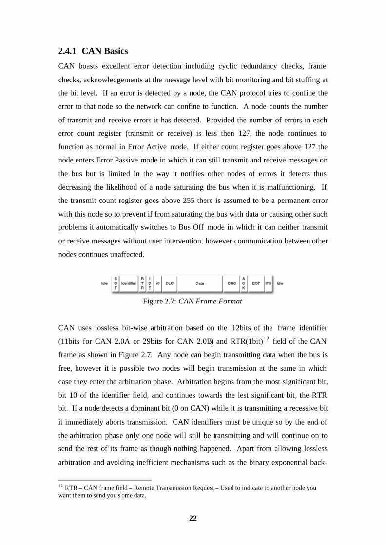
Figure 2.7: CAN Frame Format

CAN uses lossless bit-wise arbitration based on the 12bits of the frame identifier

(11bits for CAN 2.0A or 29bits for CAN 2.0B) and RTR(1bit)12 field of the CAN

frame as shown in Figure 2.7. Any node can begin transmitting data when the bus is

free, however it is possible two nodes will begin transmission at the same in which

case they enter the arbitration phase. Arbitration begins from the most significant bit,

bit 10 of the identifier field, and continues towards the lest significant bit, the RTR

bit. If a node detects a dominant bit (0 on CAN) while it is transmitting a recessive bit

it immediately aborts transmission. CAN identifiers must be unique so by the end of

the arbitration phase only one node will still be transmitting and will continue on to

send the rest of its frame as though nothing happened. Apart from allowing lossless

arbitration and avoiding inefficient mechanisms such as the binary exponential back-

12 RTR – CAN frame field – Remote Transmission Request – Used to indicate to another node you want them to send you s ome data.

23

off algorithm bit-wise arbitration allows the developer assign priority to messages

coming from certain nodes by simply giving them a low identifier. This is useful

when certain nodes, such as the ABS system in a car, need to guarantee their message

gets through as soon as possible. For further information on CAN and the CAN

standard please see reference [11] in the bibliography section.

2.4.2 CANOpen

The CAN protocol acts in layers 1 and 2 (physical and data- link) of the OSI layered

network model, the developer must write an application layer to interface the data- link

layer. A number of commercial and open application layers have been defined for

CAN, notably CAL (CAN Application Layer), CANOpen and DeviceNet. CANOpen

is used for this project for reasons stated later, so it is the only one discussed here.

Figure 2.8: CAN Network Layout

CANOpen was originally intended for motion orientated control networks but has

quickly spread to other areas. Its aim is to create standardised device profiles to

simplify a system designer’s job of integrating CANOpen enabled devices into a

CANOpen network. The idea being that devices with similar functionality but

possibly made by different manufacturers or being a different model, can be

interchanged with no alterations to the software necessary. For example there is a

CANOpen device profile for all angular encoders; under this profile the address

0x6004 will always return the current angular position of any encoder addressed,

regardless of who manufactured it.

CANOpen moves the developer away from having to deal with data frames and

implementation specific issues in favour of objects which act as a layer of abstraction

on top of data frames. In CANOpen configuration parameters and data on devices is

accessed via a standardised object index and sub-index system. Provided you have

24

the CANOpen device profile for the device being addressed, you look up the index

and sub-index of the parameter you are trying to set, or the data you are trying to

read/write, and send it across the network to the device using its identifier. For

example, the baud rate of any encoder can be set by writing the required speed to

object index 0x2100, sub- index 0 on that encoder.

CANOpen employs a number of protocols for communicating different types of

information across the network. There are protocols for the following services:

• Process Data Objects (PDOs) which are used for real time data such as a

device sending out its status. Only one CAN frame used so maximum of 8

bytes of data. This is an unconfirmed service.

• Service Data Objects (SDOs) which are used for configuration data such as

setting the baud rate of a device. There can contain up to 4 bytes of data in the

initial frame, additional data is sent in additional frames containing a

maximum of 7 bytes per frame. Each frame is individually confirmed.

• Network Management (NMT) which is used for error control, network

management and network boot-up.

• Special functions such as Sync or timestamp messages

All devices connected to the CANOpen network must implement the CANOpen

protocol stack to be able to participate in the network. For example it is not possible

to connect a standard temperature sensor directly to a CANOpen or standard CAN

network, a specific CAN/CANOpen sensor must be purchased. Alternatively one can

implement a CAN/CANOpen node using a CAN transceiver chip (such as the Philips

PCA82C251 IC), a CAN controller chip (such as the Philips SJA1000) and a

microcontroller to supply the data to the CAN controller. For the temperature sensor

example an ADC13 would be necessary to get the temperature value into the

microcontroller.

For further information on CANOpen and the CANOpen standard please see

reference [12] in the bibliography section.

13 ADC – Analogue to digital converter – Typically converts voltage levels to X-bit digital data

25

Chapter 3

Design 3.1 Overview

The project is broken into four parts; the mechanics, sensing, data acquisition and the

software. The mechanics in the project relate to the mechanical structure, including

the heavy drum, the frame to support it and additional framework needed to secure the

motorcycle in place with its rear wheel sitting on the drum. Sensing refers to the

sensors needed to allow the calculation of the dynamometer’s drum speed, detection

of the ambient environment and measurement of various engine properties such as

coolant temperature. The data from these sensors needs to be transmitted to the

monitoring computer which is what data acquisition refers to. Finally software is

needed on the monitoring computer to receive, interpret and display the data received

from the sensors via the data acquisition mechanism.

3.2 Mechanics

As discussed in section 2.2.1 there are a number of different types of dynamometers

one can use to test the power output of engines. It was decided to build an inertia

dynamometer, which utilises a heavy drum to apply a load to the engine being tested,

as there is no need for the software to control the load supplied with this type.

The main mechanical part of an inertia dynamometer is the heavy drum the rear wheel

of the motorcycle accelerates to provide a load on the engine. Consequently the

mechanical aspect of building a dynamometer centres on the drum and supporting it in

a frame such that the motorcycle could be fixed in place with its rear wheel

interfacing the drum, then when the motorcycle is accelerated it in turn accelerates the

drum. Ideally this drum will be chosen such that its moment of inertia provides a

similar load to the motorcycle engine as the engine would experience under normal

operating conditions when being accelerated down a road but as discussed in section

26

2.2.1.2 this is not essential, especially not for a proof of concept of this project as

calculating the exact drum needed would be difficult and outside the scope of the

project. The drum must be perfectly balanced for the high speed it will reach with the

motorcycle at full speed so it is important to know the maximum RPM it will reach so

the correct drum can be purchased or a fabricated drum can be properly balanced. It

is also important to know the maximum RPM of the drum so the correct bearings and

housings can be bought. The maximum RPM the drum will reach is the product of

the maximum rear wheel RPM and the gearing factor from the rear wheel to the drum

in question:

Max Drum RPM = (R / r) x Max Wheel RPM

Where R is the radius of the rear wheel including the tyre and r is the radius of the

drum, both measured in the same units. The radius of a motocross rear wheel with a

road tyre fitted is 318.15mm, the maximum speed the motocross bikes being tested

can reach is 130kilometers/hour or less. So at 130km/h the rear wheel will be

spinning at 1083RPM. Using the above formula the maximum drum RPM can be

calculated. For example a drum of radius 212.3mm will have a maximum RPM of:

(318.15 / 212.3) * 1083 = 1622RPM

The drum must have a sufficiently sturdy frame built around it to support the drum

and hold the motorcycle in place. The frame will be put under considerable load

during acceleration and braking of the drum by the motorcycle so must be fabricated

from steel and welded together. Depending on the design of the dynamometer and the

motorcycles being tested, a means of securing the motorcycle in place with its rear

wheel securely held against the drum is essential. During acceleration the motorcycle

will try to move forward off the drum and the wheel will try to move from side to side

on the drum which would be extremely dangerous unless the motorcycle is securely

fixed in place. Figure 3.1 shows a basic schematic for a motorcycle dynamometer

illustrating the key mechanical requirements.

27

Figure 3.1: Basic Dynamometer Schematic

A drum weighing roughly 300kg with a diameter of about 0.5m would suit the testing

of motocross bikes but upon contacting an engineering company it became apparent

that having a drum like this fabricated would cost considerably too much for this

project. An alternative prefabricated drum would be necessary. After a number of

weeks researching different sorts of drums already in use, ie. steam roller drums, it

was decided to use the brake drums and axle from a truck. These drums would come

already balanced for high speed (they spin at almost 1000RPM if the truck is doing

80MPH) and if the axle could be acquired with them they would be relatively easy to

mount in the dynamometer frame. To get the maximum possible moment of inertia it

was decided to use two drums, either bolted together face to face or sitting one in

front of the other in the frame with the rear wheel of the motorcycle sitting between

them.

The frame was to be a rectangle of steel welded together to hold the two drums in

place, with any additional supports needed to secure the bike in situ or sensor mounts

to be added as necessary.

3.3 Data Acquisition It was decided to use CAN for the data acquisition (transporting sensor data to the

controlling computer) part of this project because it is one of the most popular field

buses used in automation projects such as this one. It also allowed for high speed

communication and for the prioritisation of messages from certain devices, such as

28

giving the drum speed detector high priority on the bus while giving temperature

sensors lower priority.

To connect the controlling computer (a standard PC running Windows) to the CAN

bus, a CAN interface card was necessary. Fortunately the Trinity Distributed Systems

Group had a number of Softing14 CAN-AC2-PCI interface cards which are PCI cards

that simply slot into the controlling computer. The cards are supplied with hardware

drivers for Windows and API libraries for use with most programming languages. On

the backplane of the PCI card there are two RS-232 sockets for connecting up to two

separate CAN buses.

The drum speed detector (discussed in section 3.4) used for the project is a CANOpen

encoder, meaning it was necessary to use the CANOpen application layer to

communicate with it, not just plain CAN. Softing have developed an almost complete

CANOpen API for use with their CAN interface cards which they supplied to me for

use in this project. The package consists of updated Windows hardware drivers,

CANOpen Master15 API libraries, a CANOpen protocol stack, which runs on the

RISC microcontroller of the interface card and full documentation for these

components.

The CANOpen encoder will simply connect directly to the CAN bus, however to

connect temperature and humidity sensors etc. which will just be ICs16 with no CAN

support, a CAN node will need to be designed and constructed. The actual sensors to

be used are discussed in section 3.4 but the general premise is the sensors detect

whatever it is they were designed to and ind icate the value detected by supplying a

particular voltage level on their output pins. For example a temperature sensor’s

output pins might have a voltage level of 1Volt (with respect to some other voltage

level, typically referred to a Vref) to indicate -10ºC or 3.2Volts to indicate 40ºC.

Therefore to communicate a sensor’s data to the controlling PC one must first convert

this voltage level to a digital binary signal. This conversion is done by an ADC,

which can either be a discrete IC or can come built into some microcontrollers. There

will typically be a linear translation from the voltage level to the actual temperature

indicated, this translation can either be carried out by a microcontroller at the sensor

or at the controlling computer. Once the voltage level has been converted to a digital

14 Softing AG – http://www.softing.com/en 15 A CANOpen network will have a Master to deal with initialising all the nodes on the network etc. 16 IC- Integrated circuit

29

value it must be sent to the controlling computer via the CAN bus. To achieve this

one must have a microcontroller to receive the data from the ADC (most ADC chips

will have more then one analogue input so the microcontroller must also deal with

sorting and identifying the multiple signals) and handle passing the data onto a CAN

Controller IC such as the Philips SJA1000 which constructs the CAN data frames and

deals with the other aspects of communicating with the CAN bus discussed in chapter

2. The CAN controller chip must be connected to the CAN bus via a CAN transceiver

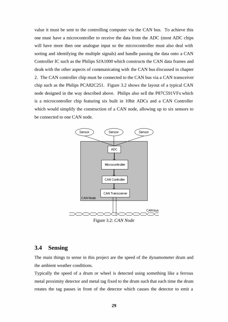
chip such as the Philips PCA82C251. Figure 3.2 shows the layout of a typical CAN

node designed in the way described above. Philips also sell the P87C591VFx which

is a microcontroller chip featuring six built in 10bit ADCs and a CAN Controller

which would simplify the construction of a CAN node, allowing up to six sensors to

be connected to one CAN node.

Figure 3.2: CAN Node

3.4 Sensing

The main things to sense in this project are the speed of the dynamometer drum and

the ambient weather conditions.

Typically the speed of a drum or wheel is detected using something like a ferrous

metal proximity detector and metal tag fixed to the drum such that each time the drum

rotates the tag passes in front of the detector which causes the detector to emit a

30

voltage pulse on its output lines. The frequency of these pulses can then be used to

calculate the drum’s speed. For this project however we required some form of speed

detector that could easily be connected to a CAN bus, hence the IVO GXP5W multi-

turn encoder shown in figure 3.3. An encoder will supply its shaft’s current angular

position when queried, a multi-turn encoder will also supply the number of times it

has gone through one full rotation, so an encoder that has been rotated 8.5 times

would reply 3060º in binary form when queried. The IVO GXP5W has a single turn

resolution of 8192, or in other words its accuracy is 0.043 of a degree while its multi-

turn accuracy is 4096 meaning it remembers the number of full turns it has been

through up to 4096, then loops back around to 0, meaning it can record up to

1,474,560º. These two values are joined together to form a 25bit output, meaning that

when the encoder is started it will output 0 as its angular position, but when it has

been rotated 4096 times its output will be decimal 33554432.

Figure 3.3: IVO Encoder

The ambient weather conditions are to be measured using basic ICs which will be

connected up to ADCs in a CAN node as discussed in section 3.3. The current

temperature can be measured using a sensor such as the LM35CAZ which features an

integrated amplifier thus providing a linear scale from the analogue voltage level (0 -

5V) to temperatures (-40ºC - 110ºC) such that a 1ºC change in temperature leads to a

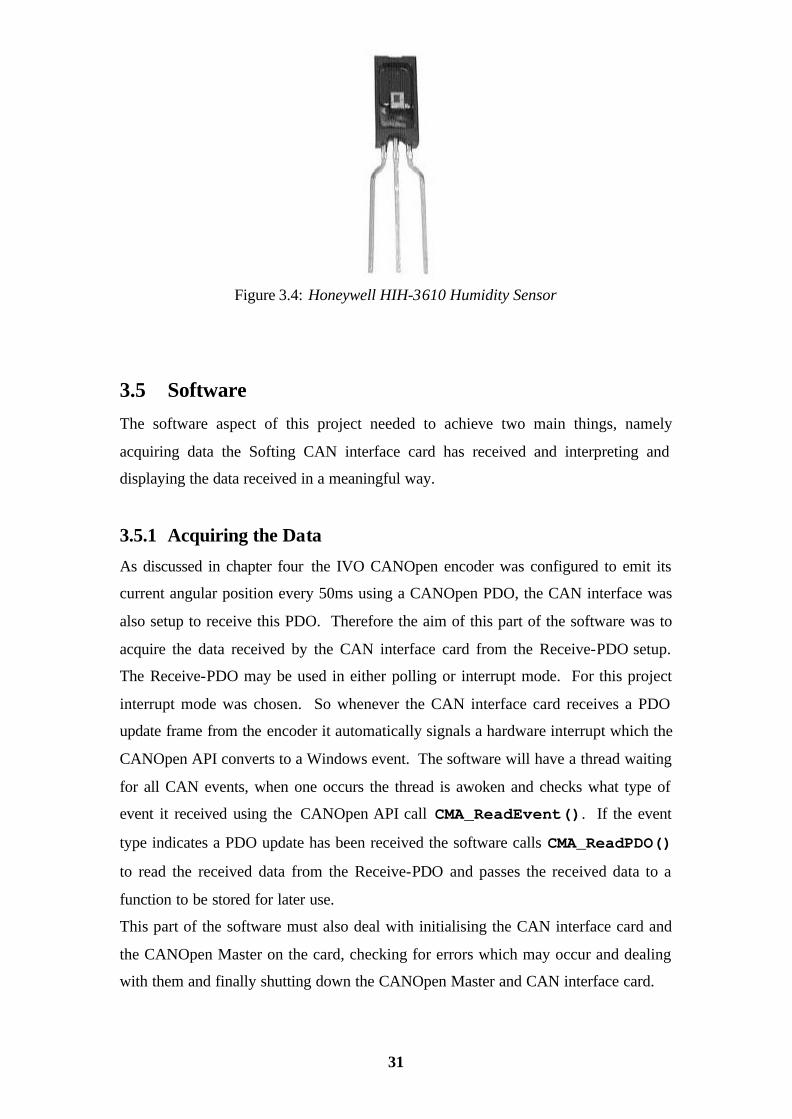
10mV change in voltage with an accuracy of +/- 0.2ºC. For humidity, a sensor such

as the Honeywell HIH-3610 Series as shown in figure 3.4 would be sufficient. This

sensor has a range from 0 – 100% relative humidity and as with the temperature

sensor above there is a linear relationship between voltage level output and the

relative humidity detected with an accuracy of +/- 2% relative humidity. Atmospheric

pressure can be measured in a similar fashion to temperature and humidity using the

Motorola MPX4115AP IC which again provides a linear analogue output. All these

sensors must be calibrated, though most can be bought pre-calibrated for a small extra

fee.

31

Figure 3.4: Honeywell HIH-3610 Humidity Sensor

3.5 Software

The software aspect of this project needed to achieve two main things, namely

acquiring data the Softing CAN interface card has received and interpreting and

displaying the data received in a meaningful way.

3.5.1 Acquiring the Data

As discussed in chapter four the IVO CANOpen encoder was configured to emit its

current angular position every 50ms using a CANOpen PDO, the CAN interface was

also setup to receive this PDO. Therefore the aim of this part of the software was to

acquire the data received by the CAN interface card from the Receive-PDO setup.

The Receive-PDO may be used in either polling or interrupt mode. For this project

interrupt mode was chosen. So whenever the CAN interface card receives a PDO

update frame from the encoder it automatically signals a hardware interrupt which the

CANOpen API converts to a Windows event. The software will have a thread waiting

for all CAN events, when one occurs the thread is awoken and checks what type of

event it received using the CANOpen API call CMA_ReadEvent(). If the event

type indicates a PDO update has been received the software calls CMA_ReadPDO()

to read the received data from the Receive-PDO and passes the received data to a

function to be stored for later use.

This part of the software must also deal with initialising the CAN interface card and

the CANOpen Master on the card, checking for errors which may occur and dealing

with them and finally shutting down the CANOpen Master and CAN interface card.

32

The Softing CANOpen Master API full documentation can be found on the included

CD-ROM in the file CMA User Manual.pdf.

3.5.2 Interpreting and Displaying the Data

The other part to the software is dealing with interpreting and displaying the data

received from the encoder. As discussed earlier the software will receive the

encoder’s angular position emitted at a specific time interval, so the type of data the

software will receive is as follows:

...31097871, 31107118, 31117821, 31129931, 31142688,

31155952, 31169632, 31183239, 31196835...

Where 31097871, for example, indicates the encoder shaft has been rotated through

3796.12º since it last reset to zero, while the next number 31107118 indicates that

50ms later it has now been rotated 3798.25º. So we now know for this example the

encoder has been turned 2.13º in 50ms, thus the angular velocity can easily be

calculated. Next 31107118 and 31117821 will be taken and the angular velocity of

the encoder during the next 50ms can be calculated, having two values for angular

velocity then angular acceleration can be deduced. From section 2.2.1 the formula for

torque can now be used to calculate the amount of torque needed to accelerate the

dynamometer drum this amount and thus the amount of torque the motorcycle engine

is producing. Knowing the angular velocities mentioned earlier the current RPM of

the engine can also be calculated for when this torque was being produced provided

the gearing factor from the encoder wheel all the way to the crank of the motorcycle

engine is known. This RPM figure and the torque figure calculated above can then be

used in the horsepower formula discussed in section 2.2.2 to calculate the horsepower

output of the motorcycle engine. The angular velocity calculated can also be used to

calculate the linear velocity of the motorcycle, if it were actually moving.

A test from idle to top RPM on a motocross bike in 4th gear takes roughly 6 seconds,

meaning the software will receive approximately 120 positions similar to the ones

above from the encoder. The data then needs to be interpreted to torque, horsepower,

RPM, speed or time and plotted on a graph so the user can see the power output of the

engine over the full range. Time/speed metrics such as RPM or speed are typically

shown on the x-axis while power metrics such as torque or horsepower are typically

shown on the y-axis. The user must have the option of changing the metrics shown on

33

each axis. To allow comparison of one test to the next the user must be able to load

multiple sets of data and have them displayed on the graph simultaneously for

comparison purposes. The data for each test run done must be saved so it can be

loaded at a later date by the user.

As discussed in section 2.3 it may be necessary to apply correction factors or smooth

the graph so the software must allow the user apply these as necessary.

34

Chapter 4

Implementation 4.1 Overview

This chapter describes the implementation of the designs discussed in chapter 3.

4.2 Mechanics The design of the mechanical aspects of the project was discussed in section 3.2.

The front brake drums and axle from a truck were acquired from a truck breakers who

also cut the axle in half, leaving the brake drums mounted to the wheel hubs which

were mounted via tapered bearings to the half axle as shown in figure 4.1.

Figure 4.1: Brake Drum and Half Axle

35

For simplicity of construction it was decided to mount the two drums one in front of

the other in the dynamometer frame, with the wheel of the motorcycle sitting between

them and effectively spinning them individually. The axles were cut down to about

12” long and AC arc welded onto short pieces of 8mm thick 8” H-section iron as seen

in figure 4.2. The two pieces of H-section were then welded onto two lengths of 8mm

thick 4” angle iron, also seen in figure 4.2

Figure 4.2: Drums Mounted to H Section

The two lengths of angle iron were then put in parallel and spaced apart by the correct

distance such that the two drum faces overlapped so the wheel of the motorcycle

could interface both of them. More lengths of 4” angle iron were then welded in place

between the two long parallel lengths to hold them together and form the rectangular

structure discussed in section 3.2 which can be seen in figure 4.3. A trial run was then

conducted using a motocross bike but it became apparent the rear wheel of the

motorcycle was going to move from side to side which would become dangerous at

high speeds. Therefore two uprights were added using more 4” angle iron in which

holes were drilled at the correct height. A 10mm threaded steel bar was then placed

through these holes and through the hollow axle of the motorcycle, nuts were then

used on the threaded bar to stop the rear wheel moving from side to side. Holes were

also drilled in the frame of the dynamometer for cargo straps to hook into and ratchet

the motorcycle down to the frame.

36

Figure 4.3: Finished Dynamometer Structure 4.3 Data Acquisition The design of the data acquisition portion of this project was discussed in section 3.3.

Although the Philips chips necessary to construct a CAN node for the temperature

sensors etc. were acquired, there was insufficient time to construct the CAN node and

implement the weather detection station. It would have been necessary to learn the

Philips assembly language to program the microcontroller but this would have taken

considerable time. It would also have been necessary to have circuit boards made up

for interconnection of the various chips necessary.

Figure 4.4: Final Data Acquisition Layout

The implementation of the drums speed pickup turned out just as designed; the

CANOpen enabled IVO encoder was connected directly to the CAN bus using a

single pair from a length of Category 5 Ethernet cable which was in turn connected to

37

the Softing CAN interface card. Another pair from the Cat5 cable was used to supply

power (10 - 30V DC) to the encoder.

4.4 Sensing

The design of the sensing part of the project was discussed in section 3.4. As

discussed in section 4.3 there was insufficient time to implement the weather

detection station so the drum speed detection was the main sensor.

The IVO GXP5W encoder has a feature to synchronously send out its current angular

position using a PDO (CANOpen Process Data Object) at a specific time interval.

This interval can be set us ing a SDO (CANOpen Service Data Object) to configure

CANOpen object 0x6200 on the encoder. After some testing it was decided 50ms

was a reasonable update interval value. So every 50ms the encoder would

automatically send out a PDO object with identifier 0x182 containing its current

angular position. The CANOpen API was then used to configure the interface card

with a Receive-PDO which acts like a register so that whenever a PDO frame is seen

on the CAN bus with an identifier of 0x182 the Receive-PDO will have its value

updated with the value found in the received PDO frame. The Receive-PDO can then

either be polled for its value or configured such that a hardware interrupt is sent to the

computer whenever the Receive-PDO is updated. 4.5 Software

The software was implemented in C++ using Microsoft’s Visual C++ 6. The

Microsoft Foundation Classes were used for the graphical user interface. 4.5.1 Acquiring the Data

The design of this aspect of the software was discussed in section 3.5.1. The

initialisation of the CAN interface card and the CANOpen Master and dealing with

receiving the Windows events signalling an event on the CAN network are all handled

in the CANController class.

An instance of this class is declared, the InitialiseCANOpen() function is then

called. This function uses the necessary CANOpen Master API calls to start the CAN

interface card and the CANOpen Master, checking as it goes for errors and handling

38

them as necessary. It also sets up the Windows event handling and starts the handler

thread which is also defined in these class files. Finally it sets up the Receive-PDO.

From this point on CANOpen events will be handled but data read from the Receive-

PDO will not be stored anywhere until the StartCapturingData() function is

called. This function is passed a pointer to a data structure (of type DynoRun which

will be discussed later) as its parameter for the CANController class to save data

received from the encoder via the Receive-PDO in. StopCapturingData() is

eventually called to cease the capture of data

4.5.2 Data Storage

The base storage structure is the RawDynoData class. It contains a vector of

integers which are basically all the angular position values received from the encoder.

Each dynamometer run loaded in the software will have one instance of the

RawDynoData class.

The other base storage structure is the Graph class. This class represents a graph,

thus it contains a linked list of 2d floating-point coordinates. It also provides some

functions relevant to graph storage and retrieval. It maintains a record of the

maximum X and Y coordinates it currently contains and provides functions to smooth

the graph.

The next level of abstraction in data storage is the DynoRun class which stores all the

information about a dynamometer run. It has an instance of the RawDynoData class

to store the raw data captured from the encoder, it also has member variables for all

other information taken at the time of the dynamometer run such as the weather data,

a name and description for the test, mechanical details such as gearing factors etc.

This class also has an instance of the Graph class which stores the current graph

representation of the run data. This is used by the GUI which will ask each instance

of the DynoRun for all the graph coordinates it should be drawing to the screen every

time the screen needs to be refreshed. The GUI will call the GetGraph() function

of the DynoRun object which will either return the current graph if it is still valid, or

if the user has changed some parameter such as the data to be shown on the X-axis

(Speed -> RPM for instance) this function will clear the Graph object and generate a

new set of coordinates based on the new parameters. The GetGraph() function is

where calculations to convert the encoder’s list of angular positions to useful data

39

such as power output will be done. Thus the DynoRun class also contains many

functions to facilitate this, such as functions for calculating angular velocity. The

DynoRun class also contains a SaveToFile() function and LoadFromFile()

function which will save or load all the data of the current dynamometer run to/from a

the file name specified as a parameter to each function. There will be one and only

one instance of the DynoRun class for each dynamometer run currently loaded in the

software, an array of DynoRun pointers is maintained by the CMainFrame object.

The CMainFrame object also has an instance of the GraphStructure class

which stores the current program settings related to graph plotting. The

GraphStructure class contains variables for information such as what data type

the X and Y axis are currently showing (horsepower, RPM, speed etc.), the current

correction factor and smoothing factor being applied and other graphical information

such as whether a grid is to be drawn over the graph.

4.5.3 Graphical User Interface

The GUI of the software is implemented with the Microsoft Foundation Classes to

implement a Single Document Interface application. Thus there is a class for each

window in the software.

The main application window is implemented in the CMainFrame class. This class

also deals with much of the control of the application, such as displaying the other

windows, maintaining a list of all the dynamometer runs currently loaded in the

software and storing graph plotting information.

The CMainFrame object also maintains the two floating options windows which

allow the user set program parameters such as the current correction factor or

smoothing factor applied (alternatively customisable via the Options menu), view a

list of the dynamometer runs currently loaded in the software, choose which runs are

currently plotted on the graph using the tick boxes next to each entry on the list or

view information about a run by double clicking on its name in the list.

The main window also contains the graph plotting area, which is implemented in the

GraphWnd class. This class contains the OnPaint() function which is called

every time the graph needs to be refreshed. The function iterates through the array of

DynoRun pointers, drawing any graphs that are selected via the graph list window.

This function deals with everything necessary to draw graph axis, the background

40

grid, the graph labels and values, the mouse target and finally the graph curves

themselves. To ensure the graph window is flicker free, especially when the mouse

cursor is moved around inside its bounds, the OnPaint() function uses double

buffering17. Thus the GraphWnd class contains a number of functions necessary for

drawing the graphs such as the PaintGraphOutline() function which does all

the calculations and drawing necessary for painting of the axis, the axis labels and the

axis values.

There are also a number of property-page style windows which appear when the user

chooses to record a new run which are all self explanatory.

Figure 4.5 shows a screenshot of the graphical user interface of the DynoSoft software

implemented. Three graphs are loaded but only two are currently selected for

drawing.

Figure 4.5: DynoSoft Screenshot

17 Double buffering – All drawing is done to an off-screen drawing context, the on-screen context is then replaced with this off-screen context in one go. This means the refresh time of the screen is equal to the time it takes to replace the current context with the off-screen one, whereas without double buffering the refresh time would equal all the time it takes to do the drawing calculations.

41

4.5.4 DynoSoft Usage

The software was implemented with the intention that recording a new dynamometer

test run be as straightforward and quick as possible. This is important because when a

tuner is running tests he/she will often run 10-15 tests in quick succession so having

to fill in pages of settings between each test would be extremely impractical.

Thus to run a test, the user must select New Run... from the File menu. The New

Dyno Run window will then appear where the user can choose any settings relevant to

the run, such as gearing information, CANOpen network parameters, weather data,

run information such as a name and description and a location to save the file to. All

these settings except for the file to save the data to have default parameters so the user

generally only needs to give the test run a name, choose a file and click the Capture

button. This will bring up the Capture window. At the top of this window is a

scrolling status box which reports status information and errors to the user. As soon

as the Capture window appears the software will start the CAN network, CANOpen

Master and the encoder so status messages will start appearing and data will begin

being received from the encoder, though not recorded yet. Under the status box is the

live info area where live information derived from the data received from the encoder

is shown. The live info area will immediately begin being updated once the CAN

network etc. has started successfully. To actually begin saving data received (ie.

when the user is about to accelerate the motorcycle) one must click the Start button,

when the bike has reached full RPM the Stop button is clicked. The dynamometer run

has now been saved to file and a graph of the data will be drawn to the screen once the

New Dyno Run and Capture windows are closed. That completes the recording of a

dynamometer test.

Loading a previously saved dynamometer run is achieved using the Open... option in

the File menu. There is also an Open icon available in the toolbar. The software

stores the four most recent ly opened run files in the system registry, these can be

opened again by simply selecting the required file from the File menu.

4.5.5 CANMan

During the configuration and testing of the CANOpen network and Ivo CANOpen

encoder it was necessary to configure the encoder using CANOpen SDO transmission

42

and test receipt of data from the encoder via PDO transmission. Thus software,

known as CANMan, was developed for the project which allowed the sending and

receiving of fully configurable SDOs and the receipt of PDO data to/from

configurable CANOpen network identifiers. The PDO data receipt mode may also be

set to polling or interrupt mode. This software can be used with any Softing CAN

interface card on any CANOpen network to configure any CANOpen device because

of its complete configurability.

In the lower portion of the main CANMan window there is a test area where

programmers may add extra fields to display data derived from data sent/received

from the CAN network. For instance in figure 4.6 the test area has a RPM field which

was programmed to display the current RPM of the encoder based on the data

received from the encoder via a configured PDO.

A screenshot of the software developed can be seen in figure 4.6. Note this software

will start but have little functionality without being connected to a fully functioning

CANOpen network via a Softing interface card.

Figure 4.6: CANMan Screenshot

43

Chapter 5

Evaluation 5.1 Critique

5.1.1 Mechanics

The mechanical aspect of the project was made considerably more difficult because of

the high cost which would have been attached to obtaining a single solid steel drum

and mounting bearings. A single steel drum as typically used in this type of

dynamometer would have been much simpler to fix into the dynamometer frame

greatly reducing the design and implementation of this phase of the project. A single

drum would also have been secured to both sides of the frame, reducing the amount of

vibration experienced during a full speed motorcycle test.

A frame to support the front wheel of the motorcycle and extra framework to allow

covers be affixed to the frame for safety and aesthetic reasons were planned but time

restrictions prevented this from being implemented.

5.1.2 Data Acquisition

CANOpen over a CAN network turned out to be a very appropriate choice for data

acquisition. However it added a considerable amount of time and work to the design

and implementation of the project overall, as I had not even heard of CAN before

commencing this project. CANOpen is a complicated concept and protocol, that is

not detailed in depth anywhere freely (ie. without paying CiA) accessible to the

general public, thus researching it was difficult and took a considerable amount of

time. There is also little detailed troubleshooting information pub licly available, so

when the CANOpen network did not work immediately, solving the problems was

difficult and time consuming.

The Softing CANOpen Master API is unfortunately not complete so there were a

number of features missing that would have simplified the implementation of the

project.

44

5.1.3 Sensing

The Ivo CANOpen encoder is well designed and reasonably well documented so once

the CANOpen network is functioning, configuring the encoder is reasonably

straightforward. There were a few initial problems such as that the default

configuration of the encoder was not what the documentation claimed it should be.

So for instance, it took some time to discover the baud rate was not what the

documentation said it would be (20kpbs) and was in fact set to 10kbps. Another issue

was the documentation did not describe how to store configuration changes made.

After much searching it transpired one must write the ASCII word “save” in reverse

(ie. 0x65766173) to SDO 0x1010 on the encoder.

The graphs plotted in the DynoSoft software were slightly noisy; I suspect, though

have not confirmed, that the timer used in the encoder to synchronously transmit its

angular position via PDO may not be accurate enough for the purpose. The vibrations

of the drum, meaning the encoder wheel was not spinning against the drum perfectly,

may also be the cause of this problem. To overcome these problems a ferrous metal

proximity detector and metal tab on the drum could be used to detect the rotations of

the drum, thus the sensor would be isolated from the drum and its vibrations.

5.1.4 Software

The software worked out very well and because of the object orientated approach used

in its design and implementation is extremely customisable to projects of a similar

nature.

The scale and depth of the software meant I used considerably more of the Microsoft

Foundation Classes and C++ then I had before, thus a considerable amount of time

was spent researching MFC classes and C++ mechanisms and how to implement

them. I had also never implemented any form of graph plotting before so this part of

the software took quite a bit of time to develop.

45

5.2 Future Work

The implementation of the mechanical aspect of the project could be built upon, such

as adding a support frame for the front wheel of the motorcycle and fabricating covers

for the dynamometer.

Completing the implementation of the additional sensors for monitoring the ambient

weather conditions and engine conditions is the most desirable future work for this

project. Correction factors for the graphs are essential for comparing tests taken on

bikes in different weather conditions or in different geographical locations.

Changing the method of sensing the dynamometer drum speed from an encoder to the

detector discussed in section 5.1.3 would also be useful future work to improve the

accuracy of the dynamometer. This would entail implementing a full CAN node as

discussed in section 3.3 that would measure the time between pulses from the detector

to microsecond accuracy and send these timings to the controlling computer over the

CAN network.

5.3 Summary

The project aim was to build a tool to aid the tuning of motorcycles by showing the

tuner the power output of an engine and allowing him/her compare this to a previous

test taken on the same engine. It was decided to use CAN as the method of

transmitting the data measured by the sensors to the controlling computer as this kind

of project is essentially what CAN was designed for. This decision added a

considerable amount of work to the project over say, using the serial port of a

computer, as I had no previous experience with CAN. Software was written to

receive the data from the CAN network and present it to the user in a meaningful way

(power graphs). The construction of the dynamometer was completed and produced

good results which, with some fine tuning, would be invaluable to a tuner.

46

5.4 Conclusions

The dynamometer is regarded as a success; it can be used in its current form as an aid

for motorcycle tuning. The tuning process would be greatly simplified by the use of

this dynamometer and the results of tuning modifications made could be verified.

47

Bibliography [1] Richard Rohrich, Fuel for thought

http://www.ericgorr.com/techarticles/Fuel_Basics.htm

[2] Eric Gorr, Two-Stroke Principles

http://www.eric-gorr.com/twostktech/2techbasicprincipals.htm

[3] A. Graham Bell, Two Stroke Performance Tuning Second Edition,

Haynes, ISBN 1859606199

[4] Marshall Brain, How Car Engines Work

http://auto.howstuffworks.com/engine.htm

[5] A. Graham Bell, Four Stroke Performance Tuning Second Edition,

Haynes, ISBN 1859604358

[6] Land & Sea, Dynamometer Comparison

http://www.land-and-sea.com/dynamometer/dynamometer-

comparison.htm

[7] Mathematica in Engineering, Mass Moment of Inertia

http://www.efunda.com/math/solids/MassMomentOfInertia.cfm

[8] Measure moment of inertia of a rotating mass experiment

http://www.edison.edu/faculty/manacheril/phy_2048/webphy2048/

Lab11.htm

48

[9] Stephen Muller and Tom Barber, Horsepower and Torque

http://home.iprimus.com.au/stevebm/dyno_02.htm

[10] Richard Shelquist, Dyno Correction Factor and Relative

Horsepower

http://wahiduddin.net/calc/cf.htm

[11] CiA, Controller Area Network (CAN), an overview

http://www.can-cia.de/can/

[12] CiA, CANOpen, an overview

http://www.can-cia.de/canopen/