Motion Planning in the Presence of Mobile Obstacles

Motion Planning in the Presence of Mobile

Obstacles

Avi (Abraham) Stiefel

Technion - Computer Science Department - M.Sc. Thesis MSC-2015-23 - 2015


Motion Planning in the Presence of Mobile Obstacles

Research Thesis

In Partial Fulfillment of The Requirements for the Degree of Master of Science in

Computer Science

Avi (Abraham) Stiefel

Submitted to the Senate of the Technion - Israel Institute of Technology

Av, 5775, Haifa, July 2015



The Research Thesis was done under the supervision of Prof. Gill Barequet in

the Faculty of Computer Science

I would like to thank Prof. Barequet for all his assistance and patience during

my research.

I would like to give a special thanks to Miriam and Azi, without whom I could

not have finished this thesis, as well as all those who have supported me through

this endeavor.



Contents

1 Introduction 3

1 Background . . . . . . . . . . . . . . . . . . . . . . . . . . . . . . . . 4

1.1 Reactive Algorithms . . . . . . . . . . . . . . . . . . . . . . . 4

1.2 Path-Based Algorithms . . . . . . . . . . . . . . . . . . . . . . 5

1.3 Site Selection . . . . . . . . . . . . . . . . . . . . . . . . . . . 5

1.4 Path Generation in Dynamic Algorithms . . . . . . . . . . . . 8

1.5 Path Smoothing . . . . . . . . . . . . . . . . . . . . . . . . . . 9

2 Terminology and Goal 11

1 Definitions . . . . . . . . . . . . . . . . . . . . . . . . . . . . . . . . . 11

2 Given . . . . . . . . . . . . . . . . . . . . . . . . . . . . . . . . . . . 12

3 Statement of the Problem . . . . . . . . . . . . . . . . . . . . . . . . 14

3 Overview of the Method 17

1 Motivation . . . . . . . . . . . . . . . . . . . . . . . . . . . . . . . . . 17

2 Method . . . . . . . . . . . . . . . . . . . . . . . . . . . . . . . . . . 17

3 Convex Decomposition of the Free Space . . . . . . . . . . . . . . . . 19

3.1 Data Structures . . . . . . . . . . . . . . . . . . . . . . . . . . 19

3.2 Definitions . . . . . . . . . . . . . . . . . . . . . . . . . . . . . 19

4 Method of Decomposition . . . . . . . . . . . . . . . . . . . . . . . . 19

4.1 Adding and Removing Gates . . . . . . . . . . . . . . . . . . . 20

4.2 Convex Decomposition of the Polygon . . . . . . . . . . . . . 20


4.3 Initialization . . . . . . . . . . . . . . . . . . . . . . . . . . . . 24

4.4 Maintaining the Convex Decomposition . . . . . . . . . . . . . 27

5 Search Graph Construction . . . . . . . . . . . . . . . . . . . . . . . 29

5.1 Structure of the Search Graph . . . . . . . . . . . . . . . . . . 29

5.2 Selection of Best Path Segments . . . . . . . . . . . . . . . . . 30

5.3 Search Graph Initialization and Update . . . . . . . . . . . . . 30

5.4 Maintaining the Graph . . . . . . . . . . . . . . . . . . . . . . 32

5.5 Full Update Process . . . . . . . . . . . . . . . . . . . . . . . 33

6 Path Augmentation . . . . . . . . . . . . . . . . . . . . . . . . . . . . 34

6.1 End-Point Orientation Computation . . . . . . . . . . . . . . 35

6.2 Curve Computation . . . . . . . . . . . . . . . . . . . . . . . . 35

7 Improvement to Path-Length Estimate . . . . . . . . . . . . . . . . . 37

8 The Complete Algorithm . . . . . . . . . . . . . . . . . . . . . . . . . 38

9 Panic Mode . . . . . . . . . . . . . . . . . . . . . . . . . . . . . . . . 38

4 Curvature Augmentation Methods 41

1 Notation . . . . . . . . . . . . . . . . . . . . . . . . . . . . . . . . . . 41

2 Circle-to-Circle Spline . . . . . . . . . . . . . . . . . . . . . . . . . . 42

2.1 Computation . . . . . . . . . . . . . . . . . . . . . . . . . . . 42

2.2 Curve Length . . . . . . . . . . . . . . . . . . . . . . . . . . . 46

2.3 Maximum Curvature . . . . . . . . . . . . . . . . . . . . . . . 47

2.4 Failure of Computation . . . . . . . . . . . . . . . . . . . . . . 47

2.5 Improvements to the Boundedness Test . . . . . . . . . . . . . 47

3 Cubic Bezier Spline . . . . . . . . . . . . . . . . . . . . . . . . . . . . 48

3.1 Computation . . . . . . . . . . . . . . . . . . . . . . . . . . . 49

3.2 Curve Length . . . . . . . . . . . . . . . . . . . . . . . . . . . 53




3.5 Improvements of the Boundedness Test . . . . . . . . . . . . . 55

4 Clothoid . . . . . . . . . . . . . . . . . . . . . . . . . . . . . . . . . . 56

4.1 Computation . . . . . . . . . . . . . . . . . . . . . . . . . . . 57

4.2 Curve Length . . . . . . . . . . . . . . . . . . . . . . . . . . . 58



4.5 Improvements of the Boundedness Test . . . . . . . . . . . . . 59

5 Analysis of the Algorithm 61

1 Correctness and Completeness . . . . . . . . . . . . . . . . . . . . . . 61

1.1 Finding an Axis of Monotonicity . . . . . . . . . . . . . . . . 61

1.2 Concave clipping . . . . . . . . . . . . . . . . . . . . . . . . . 62

1.3 Path Creation and Updates . . . . . . . . . . . . . . . . . . . 63

2 Complexity . . . . . . . . . . . . . . . . . . . . . . . . . . . . . . . . 63

2.1 Convex Decomposition . . . . . . . . . . . . . . . . . . . . . . 64

2.2 Search Graph Construction and Maintenance . . . . . . . . . 65

2.3 Path Augmentation . . . . . . . . . . . . . . . . . . . . . . . . 67

2.4 Total Complexity . . . . . . . . . . . . . . . . . . . . . . . . . 67

6 Results 69

1 Implementation . . . . . . . . . . . . . . . . . . . . . . . . . . . . . . 69

2 Convex Decomposition . . . . . . . . . . . . . . . . . . . . . . . . . . 71

2.1 Average Numbers of Polygonal Regions . . . . . . . . . . . . . 72

2.2 Complexity of the Polygons in the Decomposition . . . . . . . 73

3 Construction of the Spline Tree . . . . . . . . . . . . . . . . . . . . . 74

4 Path-Augmentation Methods . . . . . . . . . . . . . . . . . . . . . . 76

4.1 Minimum Length . . . . . . . . . . . . . . . . . . . . . . . . . 76

4.2 Full Path Length . . . . . . . . . . . . . . . . . . . . . . . . . 78

4.3 Algorithmic Failures . . . . . . . . . . . . . . . . . . . . . . . 79


7 Conclusions 81


List of Figures

2.1 An example model . . . . . . . . . . . . . . . . . . . . . . . . . . . . 15

3.1 Adding and removing gates . . . . . . . . . . . . . . . . . . . . . . . 21

3.2 Monotone polygon convex decomposition . . . . . . . . . . . . . . . . 22

3.3 Non-monotone polygon convex decomposition . . . . . . . . . . . . . 23

3.4 Finding an axis of monotonicity . . . . . . . . . . . . . . . . . . . . . 25

3.5 Elimination of all holes . . . . . . . . . . . . . . . . . . . . . . . . . . 26

3.6 Completed initialization of the algorithm . . . . . . . . . . . . . . . . 26

3.7 Adding a gate to the model . . . . . . . . . . . . . . . . . . . . . . . 28

3.8 Removing a gate from the model . . . . . . . . . . . . . . . . . . . . 28

3.9 Adding and removing gates from the model . . . . . . . . . . . . . . 28

3.10 Examples of gates with direct and indirect passthrough . . . . . . . . 31

3.11 Examples of the passthrough algorithm . . . . . . . . . . . . . . . . . 32

3.12 The first two iterations of the linear graph and path construction . . 34

3.13 An example of the endpoint orientation computation . . . . . . . . . 36

3.14 A curve scenario . . . . . . . . . . . . . . . . . . . . . . . . . . . . . 37

3.15 The panic cone and obstacle bounding-discs . . . . . . . . . . . . . . 39

4.1 CtC spline example . . . . . . . . . . . . . . . . . . . . . . . . . . . . 42

4.2 Vector winding signs +,+ . . . . . . . . . . . . . . . . . . . . . . . . 45

4.3 Vector winding signs +,- . . . . . . . . . . . . . . . . . . . . . . . . . 45

4.4 Vector winding signs -,+ . . . . . . . . . . . . . . . . . . . . . . . . . 45


4.5 Vector winding signs -,- . . . . . . . . . . . . . . . . . . . . . . . . . . 45

4.6 The CtC spline graph and path . . . . . . . . . . . . . . . . . . . . . 46

4.7 Examples of cubic Bezier curves . . . . . . . . . . . . . . . . . . . . . 49

4.8 The cubic Bezier spline graph . . . . . . . . . . . . . . . . . . . . . . 54

4.9 An example of a Clothoid . . . . . . . . . . . . . . . . . . . . . . . . 56

4.10 The first two iterations of the clothoid spline graph and path . . . . . 58

6.1 An example model . . . . . . . . . . . . . . . . . . . . . . . . . . . . 70

6.2 A screenshot of the UI . . . . . . . . . . . . . . . . . . . . . . . . . . 70

6.3 The number of polygons in the decomposition . . . . . . . . . . . . . 72

6.4 The number of convex polygons, before the maintenance stage . . . . 72

6.5 The number of monotone polygons, before the maintenance stage . . 72

6.6 The number of concave polygons, before the maintenance stage . . . . 73

6.7 The average complexity of all polygons in the decomposition . . . . . 74

6.8 The average maximum complexity of a polygon in the decomposition 74

6.9 The average size of the tree . . . . . . . . . . . . . . . . . . . . . . . 75

6.10 The number of gates created per iteration . . . . . . . . . . . . . . . 75

6.11 The number of gates destroyed per iteration . . . . . . . . . . . . . . 75

6.12 A labeled curve scenario . . . . . . . . . . . . . . . . . . . . . . . . . 76

6.13 Minimum lengths of the cubic Bezier spline . . . . . . . . . . . . . . . 77

6.14 Minimum lengths of the clothoid spline . . . . . . . . . . . . . . . . . 78


Abstract

We take a new approach to motion planning specifically designed for handling

mobile obstacles. Previous methods are modified versions of the algorithms for static

obstacles, but with speed-ups designed to ensure real-time operation. Because of this

logic, each iteration requires we completely recompute the path, based on the new

locations of the robot and the obstacles. Ideally, the algorithm should allow us to,

during each iteration, simply update the previous path based on the new configuration

of the robot and the obstacles.

We begin by dividing the area accessible to the robot, the freespace, into convex

regions. We then create perform a path search in the dual graph of this decompo-

sition, creating a piecewise-linear path stretching from the robot to the target, such

that each linear segment is fully contained within a single convex region. This path

is a greedy estimate of the shortest path; each segment is placed to minimize the

difference towards the target. Last, the path is augmented to become a smooth curve

with bounded curvature, with each segment fully contained within a convex region.

After the first iteration, we assume that only small changes need to be made to

our model to maintain a usable path. Therefore, we ensure that the convex decompo-

sition remains convex, updating if necessary. We refine our path, given the previous

state of the path and the current state of the decomposition. Last, we augment the

path again given the new geometric bounds.

We show that our method is computationally faster than pre-existing algorithms.

Furthermore, we show that because of the structure of the algorithm we can more

easily determine if the entire path avoids obstacles. We show that the under the

iterative improvements to the path, the path length always tends towards a local

minimum.

1



Chapter 1

Introduction

Motion planning of mobile platforms is the study of efficient navigation of a robot

from an initial pose to a final pose while avoiding obstacles. In general, robots

operate using a “Sense-Plan-Act”(SPA) paradigm [21]. In this model, the robot runs

a three stage loop to solve the problem. In the Sense stage, the robot uses sensors

to read all available information about itself, the world, and the robot’s location in

the world. During the Plan phase, the robot uses the information gathered from

the sensors to plan the next action to be taken. Last, in the Act stage, the robot

actually acts on the action recommended in the planning stage.

When the robot must only contend with static obstacles, obstacles that never

move, the existing algorithms include an initialization phase before the SPA loop.

In this phase, the robot reads all information available, constructs a model of the

world, constructs an optimal path based on the information, and stores this path

in memory. Once this path has been constructed, the SPA loop becomes simple.

The robot senses its current location on the path, determines the motion required

to reach the next location on the path, and performs that motion. Due to the static

nature of the problem, no updates to the path will ever be required, and so the bulk

of the calculation can be performed before the loop even begins.

In the case of moving obstacles, an initialization phase similar to that of the

static algorithms can be used. However, changes must constantly be made to the

model, and so the SPA loop becomes more complicated. In this case, the Sense and

Act stages remain the same, but the Plan stage must be changed to do more work.

In general, in the Plan stage the robot rebuilds or updates the model of the world,

constructs an optimal path according to the new world model, and determines what

motion is required to move along the new optimal path. This can be very costly,

3


and so steps must be taken to perform this task as efficiently as possible, so as to

ensure the algorithm can operate in real time.

A secondary concern of these algorithms is path smoothness. We want to en-

sure that the robot is not forced to turn with a radius of curvature less than the

capabilities of the robot. For example, car shaped robots cannot rotate in place.

Sometimes, we may want to have a smooth path even when the robot is capable of

rotating in place. Our goal, therefore, is not just to select an optimal path, but to

select a path that is optimal subject to curvature constraints.

1 Background

Motion-planning algorithms have two stages. First, the algorithm goes through an

initialization phase, in which the robot attempts to build a model of the workspace.

Next, the robot enters the SPA loop, in which the robot attempts to actually perform

the task of reaching the target.

Historically, there have been two classes of obstacle avoidance algorithms: reac-

tive and path-based. A reactive algorithm searches for the best single action given

the current state, while a path-based algorithm searches for a complete path. In gen-

eral, these algorithms are designed to handle polygonal obstacles; obstacles bounded

by free-form curves can be approximated by a polygon.

1.1 Reactive Algorithms

There are two types of reactive algorithms. The first type is based on the principle

of potential energy minimization [25]. In the initialization phase, the robot builds

a model that places an attractive force at the target, and a repulsive force on all

obstacles. Every possible location has its own value, and the robot can wander

anywhere necessary to minimize energy at each stage.

In the loop, the robot first reads in the current location. The robot then calcu-

lates the potential at all possible neighbour locations, selects the neighbour location

with minimum potential value, and moves to that location. In the static case, the

potential values at all locations in the workspace are calculated before the robot

begins moving. In the dynamic case, the potential values change as the obstacles

move. As the robot searches for the next location, the robot calculates the sum of

negative potentials imposed by the obstacles on all neighbour points, as well as the

4


potential imposed by the target, and selects the neighbour point with maximum

potential sum.

Since the forces at each location are based on the location of the obstacles, this

algorithm is by nature dynamic; a change in the location of the obstacles results in

an immediate change in the potential values throughout the workspace. Since we

are only concerned with the energy of neighboring locations, rather than the entire

workspace, computation of the optimal action is simple. However, this model is

extremely susceptible to local minima, and allows very little control over the shape

of the path.

The second type of reactive algorithm is a silhouette method [11]. In these

algorithms, the robot moves towards the target. Once the robot hits an obstacle,

the robot manoeuvres around the obstacle until it can move towards the target

again. If the obstacle moves, the robot will move with the obstacle. This algorithm

is especially unsuited for moving obstacles, because the robot spends large amounts

of time immediately adjacent to obstacles, which will lead to unintended collisions.

1.2 Path-Based Algorithms

All path-based motion planning algorithms currently in existence work along the

same principles. The algorithms use the following process:

1. Site Graph Generation: The algorithm generates a set of sites, locations in the

workspace to be used as markers or waypoints for the robot’s movement. The

algorithm also creates adjacencies between sites, creating a graph of possible

site-to-site movements.

2. Path Selection: Using the sites as a basis, the algorithm generates an optimal

path from the initial location to the final location.

1.3 Site Selection

There are currently four primary methods of site selection: motion primitives, skele-

ton methods, visibility graphs, and cell decomposition.

5


Motion Primitives

A motion primitive, as described by Likhachev [18], is a small, basic movement

that the robot can perform. Examples may include “move forward a step,” “move

forward while turning,” and many others. All possible actions are counted. Sites

in this method are all locations that can be reached by the robot by a sequence of

motion primitives. Two sites are adjacent if one site can be reached from the other

site using a single motion primitive.

This method allows for very fine control of the path. However, this method

creates a number of sites that is exponential with the size of the workspace. There-

fore, searching for an optimal path becomes extremely difficult even for a smaller

workspace, and this is very difficult to manage in a real-time manner. Further, when

directing a robot, we generally do not command the robot to go to a specific point.

In general, we tell the robot in what direction to move, at what speed, but this

algorithm would require us to give commands of start and stop to the robot. It is

much more desirable to send the robots more general movement commands, rather

then command the robot to make a specific motions.

Skeleton Methods

These algorithms attempt to construct some form of skeleton representing the free

space, and using this skeleton construct a path. The robot moves from the initial

point to the nearest point on the skeleton, traverses the skeleton until it reaches the

point nearest to the target, and then moves towards the target.

In the Generalized Voronoi Diagram (GVD) method [11], the robot constructs

the graph of all locations that are equidistant from two or more obstacles. In a

standard Voronoi Diagram, the sites are individual points, and therefore the graph

consists of straight lines. Because the obstacles are not points, the edges of the

graph are not necessarily straight lines. There are three pairs of “nearest neighbour”

pairings. The points equidistant from a vertex of one obstacle and a vertex of the

other obstacle form a straight line, as do the points equidistant from an edge of one

obstacle and an edge of a second obstacle. However, the points equidistant from a

vertex of one obstacle and an edge of the other obstacle form a parabola, defined by

a focus located at the vertex and directrix located at the edge.

In this method, sites are vertices of the GVD, all points in the workspace that

are equidistant from three or more obstacles. Adjacencies are determined by the

6


GVD: if two sites have a GVD edge connecting them, they are connected in the site

graph.

This method searches for the safest path, the path that is least likely to intersect

with an obstacle. This method also has the benefit of having relatively few sites

and edges, as the complexity of GVDs is linear with the number of vertices and

edges. Because the GVD is affected by both the vertices and edges of the polygons,

if there are n vertices then the GVD is dependent on 2n sites. Since it is known

that a regular Voronoi diagram has at most 2n − 5 vertices and 3n − 6 edges [2],

the GVD has at most 4n − 5 vertices, and at most 6n − 6 edges. In actuality, this

bound is very high, and many fewer edges and sites will be generated (any site or

edge equidistant from two or more vertices or edges from the same polygon may be

discounted). Therefore, paths based on GVDs are safe and easy to compute, once

the initial GVD is calculated.

However, Generalized Voronoi Diagrams have a number of drawbacks, making

them unsuited to the dynamic case. During an iteration of the SPA loop, the obsta-

cles may move, which can drastically change the GVD. Movement by the obstacles

can lead to large changes in the GVD, leaving the robot stuck off a path. The

robot could potentially spend a lot of time moving towards the path, rather than

the target. Further, during each iteration the algorithm must reconstruct the entire

diagram, which is not ideal. While the GVD can be computed in O(n log n) time [2],

it is still desirable to not have to fully recompute this at each iteration.

Visibility Graph (VG)

A visibility graph [11] is a graph in which the vertices are corners of the obstacles

and the workspace, and edges connect vertices if the straight line between the two

vertices does not pass through any of the obstacles. In this case, the sites are vertices,

and the adjacencies are determined by visibility.

This algorithm seeks the shortest path, a straight line. The VG of obstacles

consisting of n vertices will have exactly n sites, by definition. The number of

edges is higher, O(n2), but still low enough to create a relatively small search space.

However, This algorithm is also not truly suited for real time. First, this algorithm is

predicated on the idea of getting close to obstacles, which is risky when the obstacles

can move. Further, computation of the VG is an O(n2 log n)-time problem [2], and

can be too complex for a real-time algorithm. This algorithm also has the same

issue of repeated reconstruction of the model, which we would like to avoid.

7


Cell Decomposition

The idea of this algorithm is to divide the free space of the workspace into cells [16].

Sites are then located in free cells, and adjacencies are determined by adjacent

cells. There are a number of different algorithms that use cell decomposition. A

commonly-used algorithm is trapezoidal decomposition [27], where the free space

is divided by vertical lines. Other algorithms overlay the workspace with a grid,

and all empty regions are considered free sites. In these algorithms, the specific site

selection is not so obvious. There are a number of different possibilities, such as

the centroids of the regions. The trapezoidal decomposition can be computed in

O(n log n) time, but must be fully recomputed at each iteration as there is no easy

way to update the decomposition easily. The grid method is much more expensive

to compute; with k cells in the grid the computation of free regions takes O(kn)

time [23]. Furthermore, the grid method rules out all areas that are in grid cells that

intersect with obstacles, even the areas that are not within the obstacles themselves.

This means that we could potentially rule out a legitimate path.

1.4 Path Generation in Dynamic Algorithms

There are many algorithms that try to generate paths in real time, using the sites

found in the first part of the algorithm. In the case of Cell Decomposition, Skeleton

Methods, and Visibility Graphs, the size of the graph is linear with respect to the

size of the workspace and obstacles, and so a general heuristic search, such as A* [15],

can be used.

When using motion primitives, an exhaustive search is not fast enough to run

in real time. During each cycle, the robot must expand all possible motions, search

the entirety of the search graph, and select the currently optimal path. The number

of sites grows exponentially with the size of the workspace, and so an exhaustive

search in a large workspace would take too much time. While a real time variant

of A* has been developed [13], the algorithm still cannot successfully perform an

exhaustive search under the time constraints. There are other variants of A*, such as

D* [6], which performs a forward search and a backwards search simultaneously. D*

is faster than A*, since it only must search halfway. However, although D* is faster,

even its real-time variant is not fast enough for real-time applications. Therefore,

various algorithms have been developed to approximate an exhaustive search in a

shorter time, to ensure the algorithm can run in real time. These algorithms try to

limit the number of states to search.

8


Local Search Space Real Time A* [14], performs an exhaustive search over a

smaller region surrounding the starting location. Given a positive integer n, the

algorithm expands n states, as in A*. A modified heuristic is used, which is the

distance from the state to the nearest state that is on the edge of the opened region

added to the distance from that state to the target. The algorithm then uses the

best path in the smaller search space.

Other algorithms use probability to limit the search space. These algorithms

only open a subset of the possible states, and perform a search on the smaller set of

states. The Random exploring Random Trees [17] algorithm begins at the robot and

randomly expands the search graph to a given number of states, and then searches for

the best path in this randomly-generated search space. Probabilistic Road Maps [12]

works similarly, but instead of expanding just from the robot, the algorithm creates

a set of sites spread randomly throughout the free space of the workspace, and

expands search graphs from each of these nodes as well. This gives us many disjoint

subgraphs, and the best path within the smaller subgraphs is calculated using A*.

1.5 Path Smoothing

When using skeleton methods, visibility graphs, and cell decomposition, the result-

ing path is generally not smooth, which forces the robot to rotate in place. We

much prefer to have a smoother path that allows the robot to move constantly, and

not rotate in place. Therefore, methods have been developed to augment the path

in such a way that the path remains smooth throughout. Control points are placed

based on the path and the free space to generate a piecewise Bezier curve or B-spline

that remains within the free space [20].

9



Chapter 2

Terminology and Goal

1 Definitions

We use the following general definitions to describe the algorithm.

XA simple polygon in a 2-dimensional Euclidean space. Alternatively, a simply-connected open subset of the plane

∂XThe boundary of X, consisting of edges and vertices

|X|The complexity (number of edges/vertices) in the bounds of X

VXThe vertices of the boundary of X

EXThe edges of the boundary of X

tA real valued time parameter

Xt

X at time t

κ(x)Given a real-valued function, f(x), this is the curvature of the function at agiven point x, equal to the reciprocal of the radius of the tangent circle 1

rtan.

For a parametric function, the curvature is defined as κ(x) = ‖f ′(x)×f ′′(x)‖‖f ′(x)‖3

siteA point in the plane.

11


2 Given

For the algorithm to operate, we must know certain information. We must know

the bounds of where the robot can move, what obstacles exist and where they are,

and what the target is. Furthermore, we must know the state of the robot and the

obstacles at the current point in time. To this end, the following information must

be known.

Workspace: W ⊂ R2

The workspace is represented by a simple polygonal boundary. In general, we want to

limit our focus to a specific region, and not care about the entire world. Furthermore,

we say that the workspace is simple, so that the robot can reach the entire workspace.

If the workspace is not connected, we can treat the workspace as a number of separate

workspaces, and only concern ourself with the workspace containing the robot.

Robot: R(t) = (xR(t), yR(t)) ∈ R2, θR(t) ∈ [0, 2π]

A robot is represented by a single point and an orientation. All robots can be

represented by a single point, even if the robot itself is actually a polygon or a

circle. Polygonal robots can be represented by the minimum bounding circle of the

robot’s vertices, and a circular robot can be represented by the center of the robot.

In such a situation, we can expand all obstacles to ensure that the robot never

intersects with any obstacle. We also define v(R(t)) as the velocity of the robot at

t, and κ(R(t)) as the curvature of the path of the robot’s motion at time t.

Target: T = (xT , yT ) ∈ R2

The target is a single point in the plane. The target is static, so there is no time

parameter.

Obstacles: B(t) = {B0(t), ..., Bb(t)|Bi(t) ⊂ R2}

An obstacle is a simple polygon that the robot cannot enter. We assume that

W ∩ Bi(t) 6= ∅, that the obstacle is at least partially within the workspace, and

12


invalidates a portion of the workspace. If this is not the case, then we can discount

the obstacle as irrelevant.

A static obstacle is an obstacle that does not move. Conversely, a dynamic, or

mobile obstacle is an obstacle that translates and rotates over time. Therefore, at

any given moment the obstacles can be located at any location. We assume that

the motion is smooth; the obstacles cannot jump, and over a short period of time

the obstacles will only translate and rotate a small amount. We also assume that

this motion is random from the perspective of the robot, and that the robot cannot

predict the position of the obstacles at any particular point in time.

Path: P (τ, t) = {xp(τ, t), yp(τ, t)}

A path is a piecewise-parametric function that leads from some initial location to

some final location. The path can be any parametric function, although constraints

placed on the path can define what forms of functions may be used. For example,

if we ignore the curvature constraint and simply search for the shortest path, the

path will be a piecewise-linear function.

Time Dependence

� W is constant with respect to time, meaning the bounds of the workspace do

not change;

� T is constant with respect to time; the target point does not move (a loose

requirement);

� Each Bi translates and rotates rigidly and smoothly over time. The motion is

bounded such that, for b obstacles:

∀t,∀i ∈ [1, b], Bi(t) ⊂ W

∀t,∀i, j ∈ [1, b] Bi(t) ∩Bj(t) = ∅

� R(t) moves smoothly over time; and

� θR(t) changes smoothly over time, but is normalized to stay in the range

[−π, π].

13


3 Statement of the Problem

Given:

� A workspace, W ;

� A set of b obstacles B = {Bi}, i = 1...b;

� A robot R = (xR(t), yR(t)), with orientation θR(t);

� A target site T = (xT , yT ); and

� A maximum path curvature, α;

navigate R to the target, if possible, such that the following statements all hold

true:

� The robot site is never contained (even partially) within any of the obstacles,

∀t : (xR(t), yR(t)) /∈⋃Bi,t;

� The path of the robot is always smooth,

∀t : dxR(t)dt

, yR(t)dt

exist;

� The motion of the robot never stops completely,

∀t :

√(dxR(t)dt

)2+(dyR(t)dt

)26= 0; and

� The curvature of the path never exceeds the given threshold, or alternatively,

the robot never makes excessively sharp turns:

∀t : |κ(R)| < α.

We assume that R has perfect knowledge of the world.

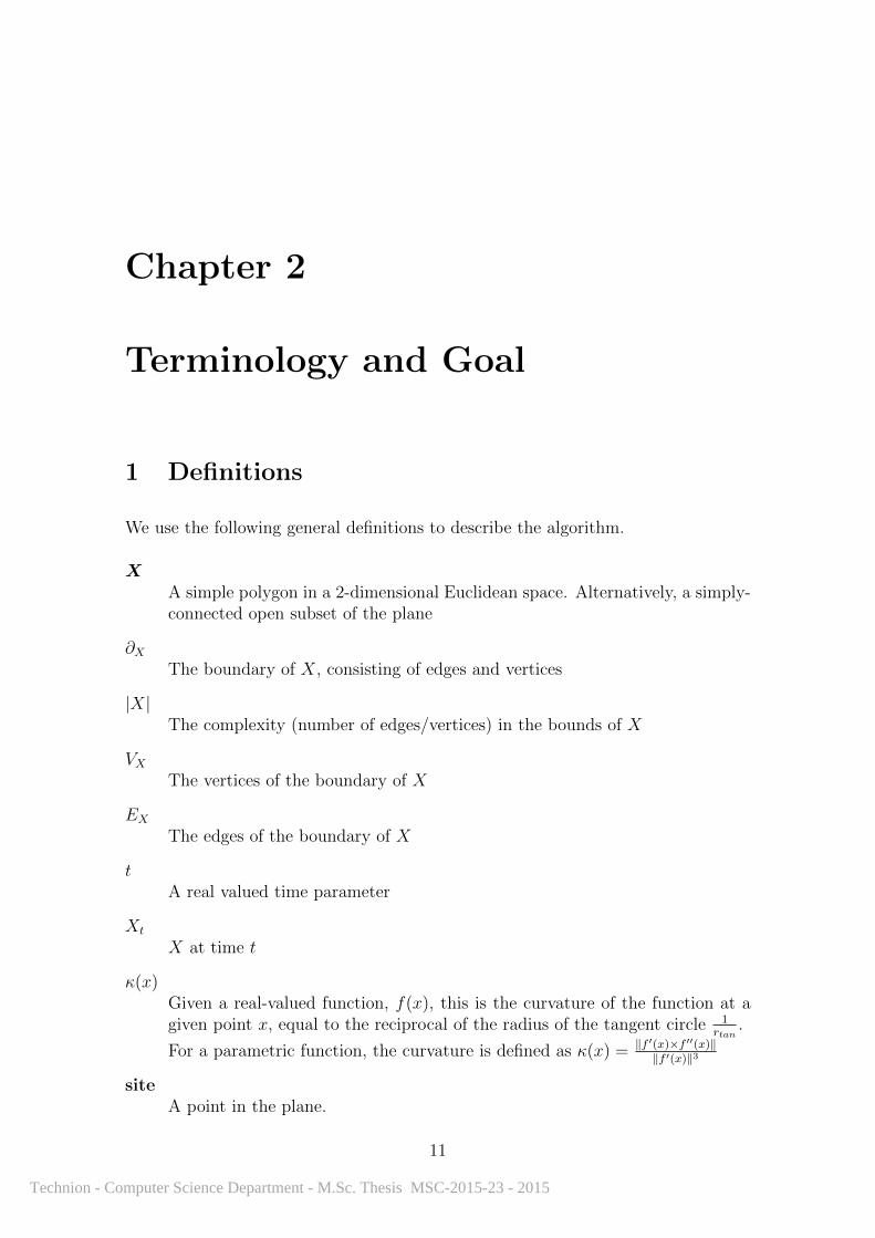
A complete layout, with a workspace, obstacles, robot, and target point, will be

called a model. Figure 2.1 shows a sample model, one which we will use throughout

this thesis. The octagonal white region, bounded by the red boundary and the grey

space, is the workspace. The red polygons are the obstacles, and so the white area

is the freespace. The red point surrounded by the green circle is the robot, and the

red point surrounded by the purple circle is the target. The arrow leaving the robot

is the initial orientation of the robot.

14


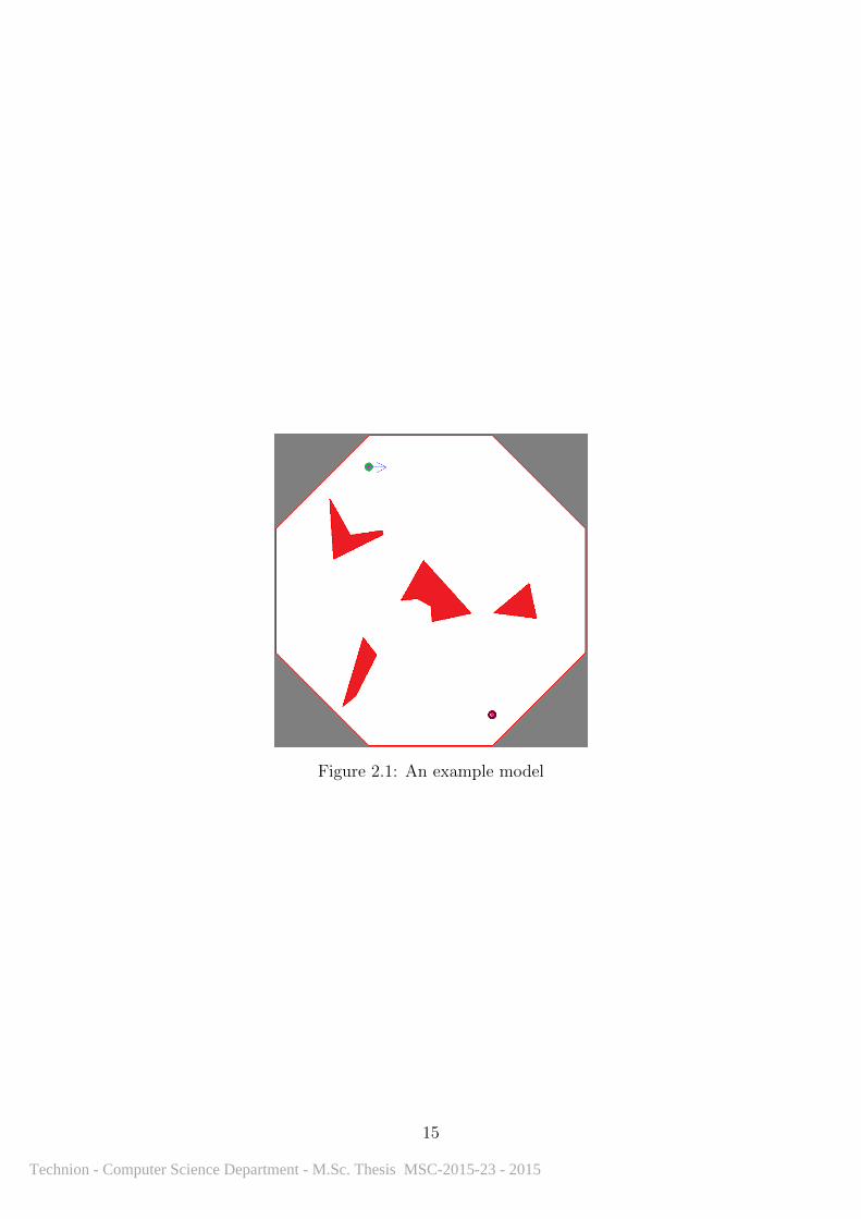
Figure 2.1: An example model

15



Chapter 3

Overview of the Method

1 Motivation

To the best of our knowledge there is no pre-existing algorithm that reuses infor-

mation from cycle to cycle, as the obstacles move. At each cycle one must entirely

recompute the visibility diagram or Voronoi diagram, or one must recheck or recom-

pute every motion primitive. Essentially, the entire process must be recomputed

fully at each iteration. To solve this problem, we separate the problem of path find-

ing into three sections that are done in sequence. We perform these steps attempting

to reuse as much information from iteration to iteration. We will then see how this

model will actually ease the path augmentation for all augmentation methods.

2 Method

The first stage of the algorithm is to create a locally-optimal convex decomposition

of the freespace. That is to say, we divide the free area, the area accessible to the

robot, into non-overlapping convex, such that no two edge-adjacent regions can be

joined into a larger convex region. This decomposition is optimal with respect to

the number of faces in the decomposition.

First, we separate the freespace into convex regions. During the first iteration of

the algorithm we add diagonals until no region is concave. We then scan through the

added edges and greedily remove unnecessary gates to create fewer, more complex

convex regions. In all other iterations of the algorithm, we attempt to maintain

as much continuity in the map. Therefore, in preparation for the next iteration,

17


after the obstacles have moved slightly, we first test each face of the pre-existing

decomposition. If the face is convex, we ignore it. If the face is now concave, we

add new edges, to separate the face into two or more convex regions. We then scan

all edges that were added in previous iterations. If the edge can be removed to fuse

two smaller convex regions into a single larger convex region, we remove the edge.

The edges that are added or removed to the model we call gates.

In the second step of the algorithm, we maintain a straight-line skeleton of the

graph, which forms a spanning tree of the adjacency graph of the faces. The straight

lines create a piecewise-linear path from the initial point to the target point. The

linear segments are joined on gates, so each segment has an initial gate and a final

gate. The spanning tree is updated backwards from the leaves (the path ends) to the

root (the robot’s current location). If two faces of the decomposition are merged,

the branches of the spanning tree are merged as necessary; similarly if a face is split,

we split the appropriate branch. When a segment is first added to the spanning

tree, the line segment is placed such that the initial point is equal to the final point

of the parent segment (on the shared gate). We place the final point on the exit

gate in such a way so as to minimize the sum of the distance from the initial point

to the final point and the distance from the final point to the target. In all other

iterations, we set the final point to match the initial point of the best child, and

then set the initial point to be the point on the initial gate that minimizes the sum

of distances from the parent’s initial point to the final point. The first branches,

whose parent is the root, have a fixed initial point, while the branches that reach

the target have a fixed final point.

In the third step of the algorithm, we recompute the path augmentation. We

select an augmentation method to create a smooth path. The method should require

as input for computation nothing more than a maximum curvature, initial and final

points, and initial and final orientations. We begin this step by computing the

initial and final orientations for each segment. The initial orientation is computed

as a function of the parent’s initial point, the initial point, and the final point, while

the final orientation is computed as a function of the initial point, the final point,

and the best child’s final point. We then compute the augmented path, based on

the selected augmentation method. We then ensure that the resulting path has a

maximum curvature less than the threshold, and is bounded within the face spanned

by the underlying linear segment.

18


3 Convex Decomposition of the Free Space

3.1 Data Structures

The convex decomposition is maintained using a doubly-connected edge list structure,

DCEL in short, which consists of the following internal structures:

Vertex

A point in R2, which contains a pointer to an outgoing halfedge.

Halfedge

A line segment in R2, exiting a source vertex. Each halfedge has a pointer

to a twin halfedge which exits the second endpoint of the line segment. Each

halfedge also contains a pointer to a preceding halfedge, a successor halfedge,

and an adjacent face.

Face

An open polygonal subspace of R2. The face contains a pointer to a single

outer, bounding edge, and a list of pointers to edges bounding ’holes,’ internal

faces.

By construction, outer halfedges of a face progress counter-clockwise around the

face, that is to say that as one traverses the boundary of a face from one halfedge

to the next halfedge, one will be traveling counter-clockwise around the perimeter

of the face.

3.2 Definitions

gate

g ∈ E, g /∈ ∂W , ∀Bi(t) ∈ B(t)→ g /∈ ∂Bi(t)

Let G be the set of all gates, G = E \ (∂W ∪⋃∂Bi(t)). Then, ∀g 6= h ∈ G, g, h

do not intersect.

4 Method of Decomposition

For the purposes of this thesis, we will refer to the set of vertices, edges, and faces as

the “model.” We will also define the term “locally-optimal convex decomposition”

19


to mean a convex decomposition such that no edge-adjacent regions can be fused

into a single larger convex region.

The primary objective of the convex decomposition method is to create and

maintain a locally-optimal convex decomposition. In the first iteration we create

the decomposition, and in each subsequent iteration we split and fuse regions as

necessary to preserve the convexity and the local optimality. A secondary objective

is to maintain continuity between iterations, where continuity is defined as similarity

between the faces at the end of the previous iteration and the current iteration. This

means that we prefer to split concave regions into a fewer number of convex regions,

rather than fully triangulate the polygon.

4.1 Adding and Removing Gates

In order to maintain a locally-optimal convex decomposition, we must be able to

easily add and remove gates from the model. Gates are added to maintain convexity,

and are removed to maintain optimality. We can view the boundary of a face as a

chain directed counter-clockwise about the face, where the links are halfedges and

the joins define the sequence of previous and next halfedges. In this model, adding a

gate is analogous to breaking two joins and adding two links to the boundary chain

to create two separate boundary chains. Similarly, removing a gate is analogous to

removing a pair set of links from two chains, and joining the broken ends to create a

single chain. In both cases, we need to maintain the correct sequence of previous and

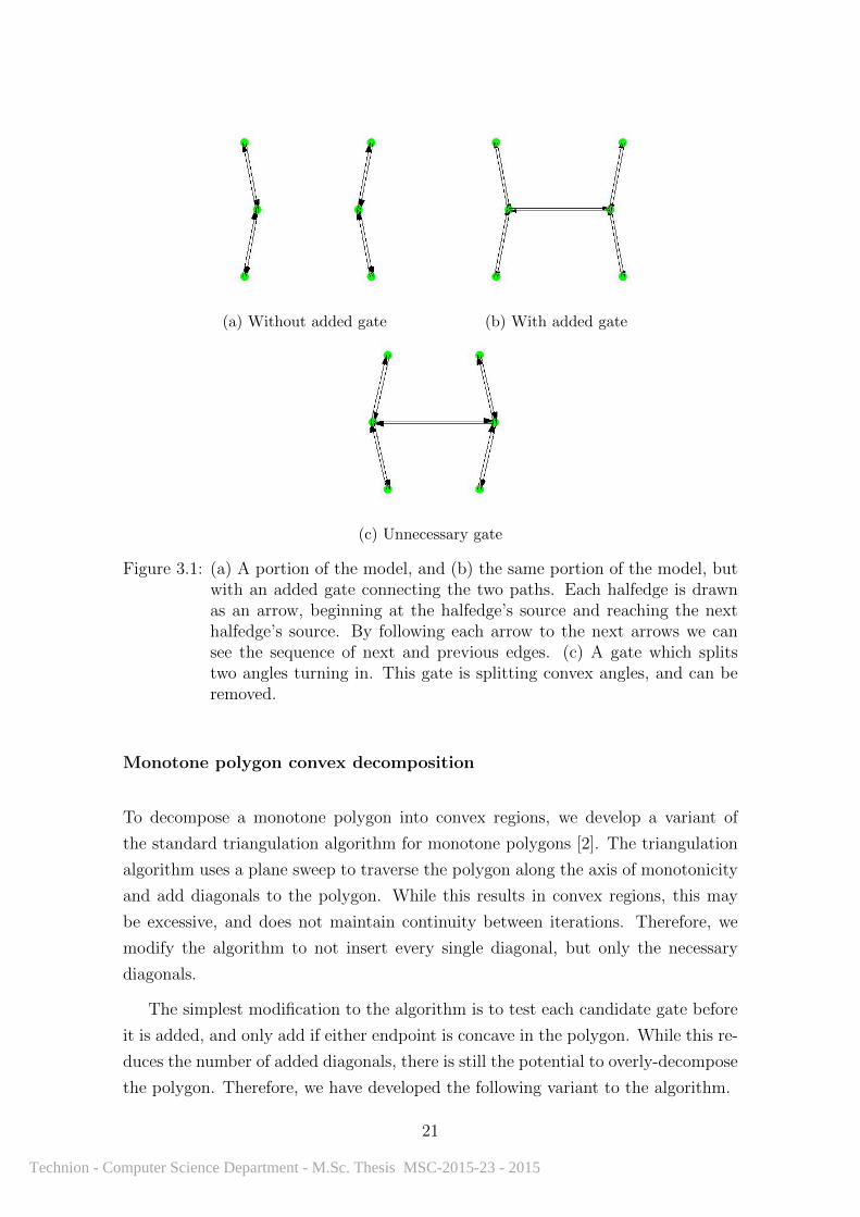
next halfedges. Figure 3.1 shows an example of necessary and unnecessary gates.

4.2 Convex Decomposition of the Polygon

In order to ensure that the decomposition results in convex regions, we must develop

a method to decompose concave polygons into two or more convex regions. Since

any polygon can be triangulated, and triangles are certainly convex, we can always

rely on this result to form a convex decomposition. However, because the goal

is to maintain a locally optimal convex decomposition, and to maintain as much

continuity as possible between iterations, we try to find a method that creates

fewer, larger convex polygons. We present different approaches for monotone and

non-monotone polygons.

20


(a) Without added gate (b) With added gate

(c) Unnecessary gate

Figure 3.1: (a) A portion of the model, and (b) the same portion of the model, butwith an added gate connecting the two paths. Each halfedge is drawnas an arrow, beginning at the halfedge’s source and reaching the nexthalfedge’s source. By following each arrow to the next arrows we cansee the sequence of next and previous edges. (c) A gate which splitstwo angles turning in. This gate is splitting convex angles, and can beremoved.

Monotone polygon convex decomposition

To decompose a monotone polygon into convex regions, we develop a variant of

the standard triangulation algorithm for monotone polygons [2]. The triangulation

algorithm uses a plane sweep to traverse the polygon along the axis of monotonicity

and add diagonals to the polygon. While this results in convex regions, this may

be excessive, and does not maintain continuity between iterations. Therefore, we

modify the algorithm to not insert every single diagonal, but only the necessary

diagonals.

The simplest modification to the algorithm is to test each candidate gate before

it is added, and only add if either endpoint is concave in the polygon. While this re-

duces the number of added diagonals, there is still the potential to overly-decompose

the polygon. Therefore, we have developed the following variant to the algorithm.

21


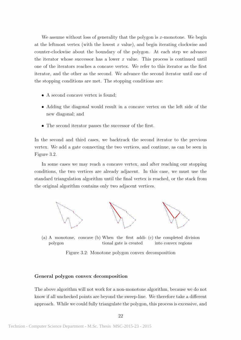
We assume without loss of generality that the polygon is x -monotone. We begin

at the leftmost vertex (with the lowest x value), and begin iterating clockwise and

counter-clockwise about the boundary of the polygon. At each step we advance

the iterator whose successor has a lower x value. This process is continued until

one of the iterators reaches a concave vertex. We refer to this iterator as the first

iterator, and the other as the second. We advance the second iterator until one of

the stopping conditions are met. The stopping conditions are:

� A second concave vertex is found;

� Adding the diagonal would result in a concave vertex on the left side of the

new diagonal; and

� The second iterator passes the successor of the first.

In the second and third cases, we backtrack the second iterator to the previous

vertex. We add a gate connecting the two vertices, and continue, as can be seen in

Figure 3.2.

In some cases we may reach a concave vertex, and after reaching our stopping

conditions, the two vertices are already adjacent. In this case, we must use the

standard triangulation algorithm until the final vertex is reached, or the stack from

the original algorithm contains only two adjacent vertices.

(a) A monotone, concavepolygon

(b) When the first addi-tional gate is created

(c) the completed divisioninto convex regions

Figure 3.2: Monotone polygon convex decomposition

General polygon convex decomposition

The above algorithm will not work for a non-monotone algorithm, because we do not

know if all unchecked points are beyond the sweep-line. We therefore take a different

approach. While we could fully triangulate the polygon, this process is excessive, and

22


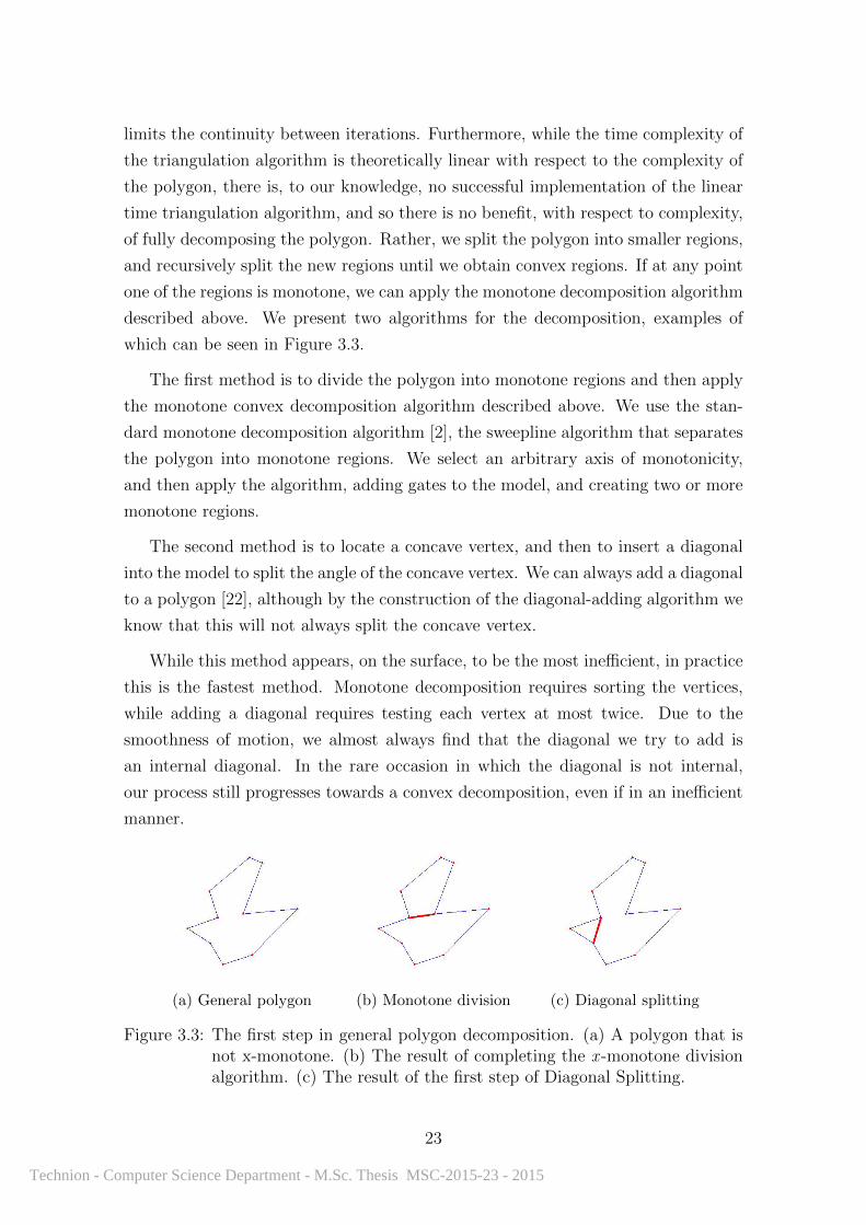
limits the continuity between iterations. Furthermore, while the time complexity of

the triangulation algorithm is theoretically linear with respect to the complexity of

the polygon, there is, to our knowledge, no successful implementation of the linear

time triangulation algorithm, and so there is no benefit, with respect to complexity,

of fully decomposing the polygon. Rather, we split the polygon into smaller regions,

and recursively split the new regions until we obtain convex regions. If at any point

one of the regions is monotone, we can apply the monotone decomposition algorithm

described above. We present two algorithms for the decomposition, examples of

which can be seen in Figure 3.3.

The first method is to divide the polygon into monotone regions and then apply

the monotone convex decomposition algorithm described above. We use the stan-

dard monotone decomposition algorithm [2], the sweepline algorithm that separates

the polygon into monotone regions. We select an arbitrary axis of monotonicity,

and then apply the algorithm, adding gates to the model, and creating two or more

monotone regions.

The second method is to locate a concave vertex, and then to insert a diagonal

into the model to split the angle of the concave vertex. We can always add a diagonal

to a polygon [22], although by the construction of the diagonal-adding algorithm we

know that this will not always split the concave vertex.

While this method appears, on the surface, to be the most inefficient, in practice

this is the fastest method. Monotone decomposition requires sorting the vertices,

while adding a diagonal requires testing each vertex at most twice. Due to the

smoothness of motion, we almost always find that the diagonal we try to add is

an internal diagonal. In the rare occasion in which the diagonal is not internal,

our process still progresses towards a convex decomposition, even if in an inefficient

manner.

(a) General polygon (b) Monotone division (c) Diagonal splitting

Figure 3.3: The first step in general polygon decomposition. (a) A polygon that isnot x-monotone. (b) The result of completing the x -monotone divisionalgorithm. (c) The result of the first step of Diagonal Splitting.

23


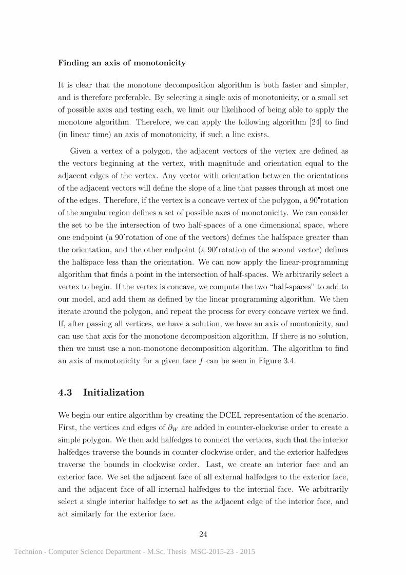
Finding an axis of monotonicity

It is clear that the monotone decomposition algorithm is both faster and simpler,

and is therefore preferable. By selecting a single axis of monotonicity, or a small set

of possible axes and testing each, we limit our likelihood of being able to apply the

monotone algorithm. Therefore, we can apply the following algorithm [24] to find

(in linear time) an axis of monotonicity, if such a line exists.

Given a vertex of a polygon, the adjacent vectors of the vertex are defined as

the vectors beginning at the vertex, with magnitude and orientation equal to the

adjacent edges of the vertex. Any vector with orientation between the orientations

of the adjacent vectors will define the slope of a line that passes through at most one

of the edges. Therefore, if the vertex is a concave vertex of the polygon, a 90°rotation

of the angular region defines a set of possible axes of monotonicity. We can consider

the set to be the intersection of two half-spaces of a one dimensional space, where

one endpoint (a 90°rotation of one of the vectors) defines the halfspace greater than

the orientation, and the other endpoint (a 90°rotation of the second vector) defines

the halfspace less than the orientation. We can now apply the linear-programming

algorithm that finds a point in the intersection of half-spaces. We arbitrarily select a

vertex to begin. If the vertex is concave, we compute the two “half-spaces” to add to

our model, and add them as defined by the linear programming algorithm. We then

iterate around the polygon, and repeat the process for every concave vertex we find.

If, after passing all vertices, we have a solution, we have an axis of montonicity, and

can use that axis for the monotone decomposition algorithm. If there is no solution,

then we must use a non-monotone decomposition algorithm. The algorithm to find

an axis of monotonicity for a given face f can be seen in Figure 3.4.

4.3 Initialization

We begin our entire algorithm by creating the DCEL representation of the scenario.

First, the vertices and edges of ∂W are added in counter-clockwise order to create a

simple polygon. We then add halfedges to connect the vertices, such that the interior

halfedges traverse the bounds in counter-clockwise order, and the exterior halfedges

traverse the bounds in clockwise order. Last, we create an interior face and an

exterior face. We set the adjacent face of all external halfedges to the exterior face,

and the adjacent face of all internal halfedges to the internal face. We arbitrarily

select a single interior halfedge to set as the adjacent edge of the interior face, and

act similarly for the exterior face.

24


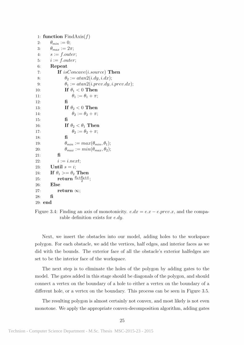
1: function FindAxis(f)2: θmin := 0;3: θmax := 2π;4: s := f.outer;5: i := f.outer;6: Repeat7: If isConcave(i.source) Then8: θ2 := atan2(i.dy, i.dx);9: θ1 := atan2(i.prev.dy, i.prev.dx);

10: If θ1 < 0 Then11: θ1 := θ1 + π;12: fi13: If θ2 < 0 Then14: θ2 := θ2 + π;15: fi16: If θ2 < θ1 Then17: θ2 := θ2 + π;18: fi19: θmin := max(θmin, θ1);20: θmax := min(θmax, θ2);21: fi22: i := i.next;23: Until s = i;24: If θ1 >= θ2 Then25: return θ1+θ2+π

2;

26: Else27: return ∞;28: fi29: end

Figure 3.4: Finding an axis of monotonicity. e.dx = e.x− e.prev.x, and the compa-rable definition exists for e.dy.

Next, we insert the obstacles into our model, adding holes to the workspace

polygon. For each obstacle, we add the vertices, half edges, and interior faces as we

did with the bounds. The exterior face of all the obstacle’s exterior halfedges are

set to be the interior face of the workspace.

The next step is to eliminate the holes of the polygon by adding gates to the

model. The gates added in this stage should be diagonals of the polygon, and should

connect a vertex on the boundary of a hole to either a vertex on the boundary of a

different hole, or a vertex on the boundary. This process can be seen in Figure 3.5.

The resulting polygon is almost certainly not convex, and most likely is not even

monotone. We apply the appropriate convex-decomposition algorithm, adding gates

25


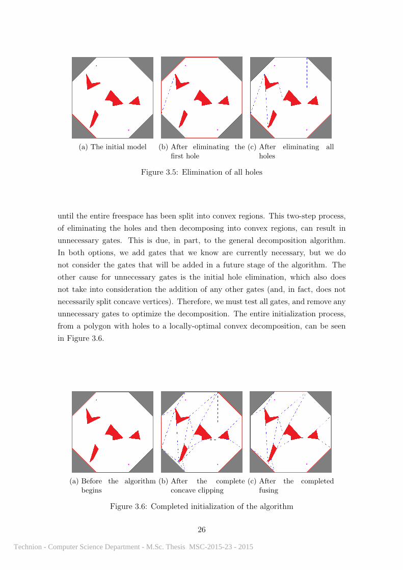
(a) The initial model (b) After eliminating thefirst hole

(c) After eliminating allholes

Figure 3.5: Elimination of all holes

until the entire freespace has been split into convex regions. This two-step process,

of eliminating the holes and then decomposing into convex regions, can result in

unnecessary gates. This is due, in part, to the general decomposition algorithm.

In both options, we add gates that we know are currently necessary, but we do

not consider the gates that will be added in a future stage of the algorithm. The

other cause for unnecessary gates is the initial hole elimination, which also does

not take into consideration the addition of any other gates (and, in fact, does not

necessarily split concave vertices). Therefore, we must test all gates, and remove any

unnecessary gates to optimize the decomposition. The entire initialization process,

from a polygon with holes to a locally-optimal convex decomposition, can be seen

in Figure 3.6.

(a) Before the algorithmbegins

(b) After the completeconcave clipping

(c) After the completedfusing

Figure 3.6: Completed initialization of the algorithm

26


4.4 Maintaining the Convex Decomposition

Because the obstacles move smoothly over time, we assume that the model can

remain fairly consistent, with few changes from iteration to iteration. Therefore,

after the initialization process we no longer have to do the process described above,

and instead can try to maintain the decomposition with as much continuity as

possible. We run a two-step process to ensure that convexity is maintained, while

keeping as much similarity between the regions before and after the process as

possible and keeping the composition locally optimal.

In the first stage we ensure that no face is concave. We begin by testing each

face for convexity and monotonicity, as described above. All concave polygons are

split using the appropriate algoritmm. In the second stage, we scan over all the

gates, and greedily remove as many gates as possible, resulting in a locally optimal

convex decomposition.

Below, Figure 3.7 shows the addition of a gate to the model, Figure 3.8 shows

the removal of a gate, and Figure 3.9 we see both actions occurring in the same

iteration.

27


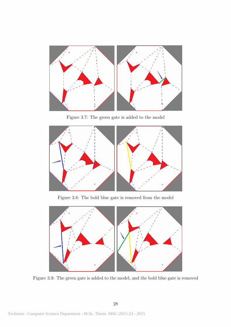
Figure 3.7: The green gate is added to the model

Figure 3.8: The bold blue gate is removed from the model

Figure 3.9: The green gate is added to the model, and the bold blue gate is removed

28


5 Search Graph Construction

The next step of the algorithm, after the convex decomposition, is to construct a

piecewise-linear tree, or skeleton, that forms the basis of our path. We will represent

the skeleton as a directed graph, or digraph, where each node represents a gate, the

robot, or the target, and edges represent linear path segments. The edges must

keep track of their initial and final points, and update as necessary. The “root” of

the digraph should be the robot, and the digraph should span the workspace, such

that the end-nodes of the graph are either ends of the searched graph, or the target.

Each edge of the graph should span a single region. During each iteration, we must

remove nodes representing gates that were removed in convex fusions, and we must

add nodes and split edges when faces are split. We must update all the edges initial

and final points.

5.1 Structure of the Search Graph

The graph consists of nodes and edges. Almost all nodes represent gates of the

convex decomposition, the exceptions being one node that represents the initial

point, the robot, and one node that represents the target. All paths on the directed

graph originate at the robot, and so we will call this the root of the graph. Edges

of the graph represent sections of the path that span a single face of the convex

decomposition, and are directed from the robot towards the target. Edges that

leave a node are called outgoing edges, and edges that come in are called incoming

edges. The node that an edge leaves is called the source node, and the node that an

edge reaches is the end node. Since gates are twinned pairs of halfedges, the node

specifically represents the halfedge adjacent to the spanning face of the incoming

edges.

Generally, in global motion-planning algorithms, the nodes of the search graph

represent specific locations in the workspace. In our algorithm, with the exception of

the root and target nodes, the nodes represent gates in G, which are line segments,

and the path segments can meet anywhere on the line segment. Therefore, each edge

of the digraph must also maintain the initial and final points on the gate segment.

Nodes keep track of the gate they represent, as well as a list of outgoing edges

of the digraph. As stated above, each edge stores the initial and final points, the

locations where the path segment begins and ends. Each edge also tracks the node

on which it ends. Last, each edge keeps track of the parent edge, the edge of the

29


digraph that leads immediately to this edge, as well a list of children, edges that

follow directly from this edge of the digraph.

We can then define the data structures and data stored in each.

� Node

– Gate halfedge g

– Outgoing edges out

� Edge

– Parent edge p

– A list of children edges children

– End node end

– Initial Point P0

– Final Point P1

5.2 Selection of Best Path Segments

By construction of the dual graph, a given edge may have more than one child edge.

Each edge must end at a single specific point, and to construct a complete path

we need the end of an edge to coincide with the beginning of the child edge that

will complete the path. Therefore, we need to determine an evaluation method that

selects a best child. For a given edge e, for each child f ∈ e.children we give f the

score of the sum of the length of f and the distance of f to the target; formally, the

f ’s score is equal to ‖f.P1 − f.P0‖ + ‖T − f.P1‖, where T is the target. We select

the child with the minimum score as the best child.

5.3 Search Graph Initialization and Update

As mentioned above, an edge of the graph and the source and end nodes are not

sufficient to represent the edge’s actual position in the plane. Because the nodes

represent line segments, and each edge passes between two nodes, we must find a

way to determine the specific locations on the nodes’ gates where the edge begins

and ends.

Furthermore, when we construct the search graph we do not want to add every

single possible edge; to do so would be to add unnecessary complexity to the search

30


graph itself, and would add unnecessary computation time to our algorithm as we

update edges that are not even searched. Therefore, we only add edges as dictated

by the graph search. As we reach a new node in our search of the graph, we add

edges to our graph connecting the node to its neighbors. If the edge already exists

from some previous iteration, we update the edge’s initial and final points based on

the new geometry.

We present the method of inserting and updating edges in the graph to find

the best possible path skeleton. Our goal in this section is to begin with a greedy

estimate of the shortest path, and iteratively improve the estimate.

As an edge is added to the search graph, the end-points are placed minimize

the distance to the target. For an edge, e, the initial point, e.P0 is set to equal

e.parent.P1 (unless e exits the root of the digraph, the robot, in which case e.P0 :=

R). Once e.P0 is set, we e.P1 is set to give the best greedy estimate of the path.

If e.end = T , e ends at the target, then obviously e.P1 := T . Otherwise, the final

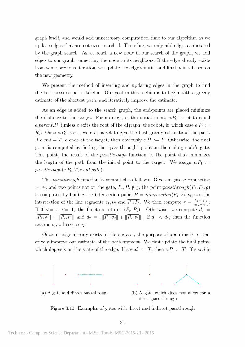
point is computed by finding the “pass-through” point on the ending node’s gate.

This point, the result of the passthrough function, is the point that minimizes

the length of the path from the initial point to the target. We assign e.P1 :=

passthrough(e.P0, T, e.out.gate).

The passthrough function is computed as follows. Given a gate g connecting

v1, v2, and two points not on the gate, Pa, Pb /∈ g, the point passthrough(P1, P2, g)

is computed by finding the intersection point P = intersection(Pa, Pb, v1, v2), the

intersection of the line segments v1, v2 and Pa, Pb. We then compute τ = Px−v1,xv2,x−v1,x .

If 0 <= τ <= 1, the function returns (Px, Py). Otherwise, we compute d1 =

‖P1, v1‖ + ‖P2, v1‖ and d2 = ‖‖P1, v2‖ + ‖P2, v2‖. If d1 < d2, then the function

returns v1, otherwise v2.

Once an edge already exists in the digraph, the purpose of updating is to iter-

atively improve our estimate of the path segment. We first update the final point,

which depends on the state of the edge. If e.end == T , then e.P1 := T . If e.end is

(a) A gate and direct pass-through (b) A gate which does not allow for adirect pass-through

Figure 3.10: Examples of gates with direct and indirect passthrough

31


not the target, but e.children is empty, we assign e.P1 := passthrough(e.P0, T, e.end).

If, however, e.children is not empty, we select the best child, and set e.P1 :=

bestChild.P0. Next, we update the initial point. If e.parent.end is the root, then

P0 := R(t). Otherwise, e.P0 := passthrough(e.parent.P0, e.P1, e.parent.end.gate).

(a) Random initialization with di-rect passthrough

(b) Initialization using passthrough

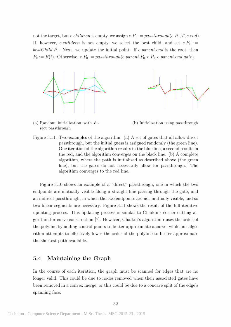
Figure 3.11: Two examples of the algorithm. (a) A set of gates that all allow directpassthrough, but the initial guess is assigned randomly (the green line).One iteration of the algorithm results in the blue line, a second results inthe red, and the algorithm converges on the black line. (b) A completealgorithm, where the path is initialized as described above (the greenline), but the gates do not necessarily allow for passthrough. Thealgorithm converges to the red line.

Figure 3.10 shows an example of a “direct” passthrough, one in which the two

endpoints are mutually visible along a straight line passing through the gate, and

an indirect passthrough, in which the two endpoints are not mutually visible, and so

two linear segments are necessary. Figure 3.11 shows the result of the full iterative

updating process. This updating process is similar to Chaikin’s corner cutting al-

gorithm for curve construction [7]. However, Chaikin’s algorithm raises the order of

the polyline by adding control points to better approximate a curve, while our algo-

rithm attempts to effectively lower the order of the polyline to better approximate

the shortest path available.

5.4 Maintaining the Graph

In the course of each iteration, the graph must be scanned for edges that are no

longer valid. This could be due to nodes removed when their associated gates have

been removed in a convex merge, or this could be due to a concave split of the edge’s

spanning face.

32


We first check for edges that end on nodes that no longer exist. Because the node

was removed as part of a convex merge, the children edges are now meant to span

the same face, and so they can be kept, but pulled one level up the digraph. We

begin at the root edge of the digraph, at the edge that is incoming to the root node.

We call the current edge current, and begin testing each child edge. For each child

edge, e ∈ current.children, we test to see if e.end.gate still exists. If e.end.gate

does not exist, then all of e.children are added to current.children. Furthermore,

for each f ∈ e.children, we assign f.parent = e.parent. Then, we assign the

initial point of f as described above. Last, we remove e from e.parent.children and

e.entranceNode.leaving. Once we complete the test on all edges, we iterate over all

edges e ∈ current.children, and recursively apply this function to e.

Next, we search the graph for edges that span split faces. Again, we begin at

the root edge, and treat it as current. For each edge e ∈ current.children, we

test if e.exitNode.adjacentFace = e.parent.exitNode.g.twin.adjacentFace (in the

case of edges leaving the root, we test if e.exitNode.adjacentFace contains the root

location). If e fails this test, then we know the spanning face was split. We add e

to a set of split edges, split, and remove them from current.children. We create

a new node, g′, representing the added gate, and a new edge e′. e′ is added to

current.children, e′.parent := current, and e′.end := g′. Then, for all f ∈ split, we

add f to e′.children, and set f.parent := e′. We then set e′.P0 := current.P1, and

we maintain f.P1 for all the edges that were split. Next, for all f , we select the best

child (as described above), and update f.P0.

It is to our benefit to prevent cycles in the search graph; partly, cycles increase

the complexity of the search graph, and partly cycles serve very little purpose, as

they require unnecessary traveling, which would guarantee a longer than necessary

path. Therefore, if two paths reach the same node, we only keep the better of the

two paths. We do not remove the entire second path, just the section that reached

the conflicted node, as well as children. This means that two segments cannot arrive

at the same gate, and thus there are no possible cycles.

5.5 Full Update Process

The full update function is a recursive, depth-first traversal that allows us to clean

and update the graph in one scan. Beginning at the root edge, we begin applying

the cleaning function described above. Before we return from a branch, and go one

level up the digraph, we select the best child. If there are no children, then there is

33


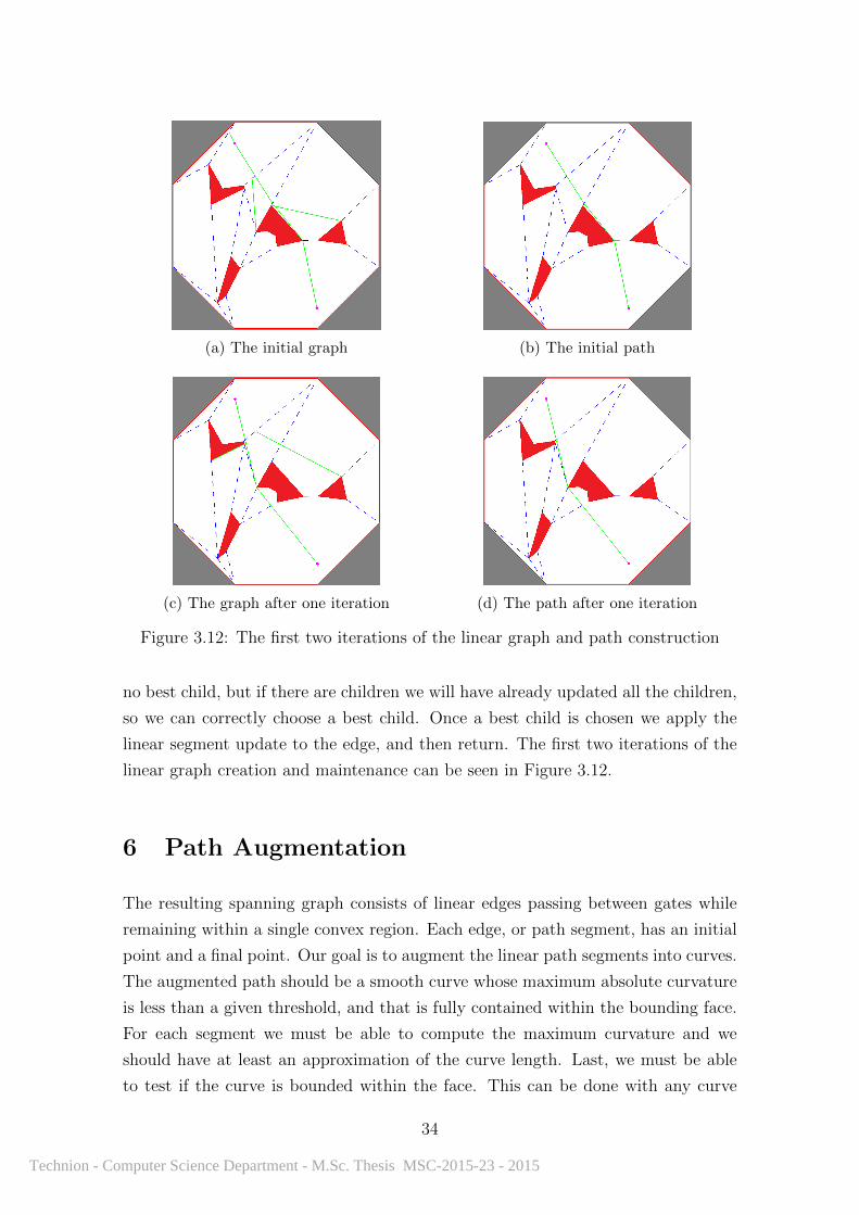
(a) The initial graph (b) The initial path

(c) The graph after one iteration (d) The path after one iteration

Figure 3.12: The first two iterations of the linear graph and path construction

no best child, but if there are children we will have already updated all the children,

so we can correctly choose a best child. Once a best child is chosen we apply the

linear segment update to the edge, and then return. The first two iterations of the

linear graph creation and maintenance can be seen in Figure 3.12.

6 Path Augmentation

The resulting spanning graph consists of linear edges passing between gates while

remaining within a single convex region. Each edge, or path segment, has an initial

point and a final point. Our goal is to augment the linear path segments into curves.

The augmented path should be a smooth curve whose maximum absolute curvature

is less than a given threshold, and that is fully contained within the bounding face.

For each segment we must be able to compute the maximum curvature and we

should have at least an approximation of the curve length. Last, we must be able

to test if the curve is bounded within the face. This can be done with any curve

34


in any polygonal face, but we will use the geometry and convexity of the faces to

accelerate the boundedness test.

6.1 End-Point Orientation Computation

The first step in computing the path augmentation is to find the initial and final

orientations of the curve segment. We have already fixed the initial and final points,

we have fixed the parent initial point and best child final point, and so from this

we can compute the orientations. The general orientation update function is the

following. Given three points, P, Pprev, Pnext, then the orientation at P , denoted by

θ, is computed as:

θ = arccos

(‖ < vprev, vnext > ‖‖vprev‖‖vnext‖

)+π

2.

where vprev = P − Pprev and vnext = P − Pnext.

We will call this calculation HeadingatPoint(P, Pprev, Pnext), and an example

can be seen in Figure 3.13.

We also add initial and final orientations to the linear segments, which we will

label, for a given segment e, by e.θ0 and e.θ1, respectively.

For a linear segment e, we set the initial heading and final headings:

e.θ0 := HeadingatPoint(e.P0, e.parent.P0, e.P1),

e.θ1 := HeadingatPoint(e.P1, e.P0, e.bestChild.P1).

If e.parent.end = root, then there is no previous point, and so we set e.θ0 := θR,

the robot’s orientation. Similarly, if e.end = target, then we have no next point,

and so we set e.θ1 to equal some final orientation (which can be chosen by the

user, or can be a function of the path and the augmentation method). Other-

wise, if e.children is empty, again we have no next point, so we assign e.θ1 :=

HeadingatPoint(e.P1, e.P0, target.point).

6.2 Curve Computation

From the construction of the skeleton, each segment has an initial point and a final

point, as well as an initial orientation and a final orientation (which for now we

35


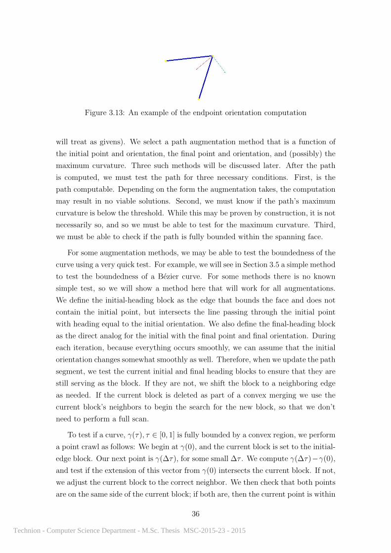
Figure 3.13: An example of the endpoint orientation computation

will treat as givens). We select a path augmentation method that is a function of

the initial point and orientation, the final point and orientation, and (possibly) the

maximum curvature. Three such methods will be discussed later. After the path

is computed, we must test the path for three necessary conditions. First, is the

path computable. Depending on the form the augmentation takes, the computation

may result in no viable solutions. Second, we must know if the path’s maximum

curvature is below the threshold. While this may be proven by construction, it is not

necessarily so, and so we must be able to test for the maximum curvature. Third,

we must be able to check if the path is fully bounded within the spanning face.

For some augmentation methods, we may be able to test the boundedness of the

curve using a very quick test. For example, we will see in Section 3.5 a simple method

to test the boundedness of a Bezier curve. For some methods there is no known

simple test, so we will show a method here that will work for all augmentations.

We define the initial-heading block as the edge that bounds the face and does not

contain the initial point, but intersects the line passing through the initial point

with heading equal to the initial orientation. We also define the final-heading block

as the direct analog for the initial with the final point and final orientation. During

each iteration, because everything occurs smoothly, we can assume that the initial

orientation changes somewhat smoothly as well. Therefore, when we update the path

segment, we test the current initial and final heading blocks to ensure that they are

still serving as the block. If they are not, we shift the block to a neighboring edge

as needed. If the current block is deleted as part of a convex merging we use the

current block’s neighbors to begin the search for the new block, so that we don’t

need to perform a full scan.

To test if a curve, γ(τ), τ ∈ [0, 1] is fully bounded by a convex region, we perform

a point crawl as follows: We begin at γ(0), and the current block is set to the initial-

edge block. Our next point is γ(∆τ), for some small ∆τ . We compute γ(∆τ)−γ(0),

and test if the extension of this vector from γ(0) intersects the current block. If not,

we adjust the current block to the correct neighbor. We then check that both points

are on the same side of the current block; if both are, then the current point is within

36


(a) A curve scenario (b) A possible curve (c) Point crawl

Figure 3.14: (a) A curve scenario, consisting of the bounding polygon, as well as theinitial and final points, orientations and heading blocks. (b) A possiblecurve, given the scenario. (c) A few steps of the crawl.

the face. We then set τ = ∆τ , and repeat the process for γ(τ) and γ(τ + ∆τ). We

repeat this process until we reach the final point, or until our two test points or on

opposite sides of the current block.

Figure 3.14 shows a curve segment scenario. We see the bounding face, as well

as the initial and final points and orientations. We also see a possible curve for

the scenario, and how the point crawl could be performed on this curve with this

scenario.

7 Improvement to Path-Length Estimate

To this point we have not discussed any specific curve augmentation method. How-

ever, based on our assumptions we know that regardless of the augmentation method

we can compute the curve length, maximum curvature, and boundedness. There-

fore, we know that we can improve our path estimation from above to include these

three factors. Rather than using the linear segment length during the full update

stage of the algorithm, we use the length of the augmented curve segment. If we

cannot augment the edge, if the augmentation function fails for some reason on a

given edge, we add a penalty to that edge’s score. We also add a penalty to the

scores of edges that violate either the curvature constraint or the boundedness con-

straint. As the scenario changes, the segments that are currently in violation of

our conditions may become compliant with said conditions, and it is to our benefit

to keep updating the curve. Therefore, we don’t destroy the segments, but keep

updating them, doing, however, our best to avoid them.

37


8 The Complete Algorithm

We first maintain the convex decomposition, as described in the first section, and

update the current face (the face of the decomposition in which the robot currently

stands). Then we run the complete graph-update function. When we update the

segments, we don’t just update the linear segments, but also update the curves, and

test the curve segments for computability and boundedness. We use the results to

update the path segments. We then run an A* search, using the curve lengths and

the penalties as the path length, and Euclidean distance from the final point to the

target as our heuristic. In this stage we can create new segments.

Once we have selected a path, we have the robot traverse the path. The robot

follows the selected path, along the initial path segment. If the robot crosses an edge

into a new region, we need to update the graph. We select the best child of the first

path segment as the next step in the path. We move into the region and rebalance

the tree. If the first segment is e, and the second segment is f , then we apply the

following process: we flip e.gate, to use the gate edge twin. We then remove f from

e.children, and add e to f.children.

The algorithm terminates when the robot cannot travel any longer. This occurs

when either the robot reaches the target, or the robot cannot reach the target (if

the obstacles trap the robot).

9 Panic Mode

There are two possible scenarios by which we may have to break out of the standard

algorithm. The first situation is when the initial segment fails one of the three tests:

thresholded curvature, boundedness, or computability. If any of these tests fail, then

we choose a direction of rotation, and turn at maximum curvature in that direction

of rotation until the path passes all three tests. The second possible situation is if

the robot comes too near an obstacle. In that case, we turn away from the obstacle

at maximum curvature.

In order to determine that we are nearing an obstacle, that a collision is immi-

nent, we define a cone in front of the robot, which we will call the panic cone. This

cone has a known aperture angle and known side-length. We can test if the robot

is nearing the boundary of the workspace by checking all edges of the boundary of

the workspace, e ∈ EW . If any edge intersects the panic cone, then the robot enters

38


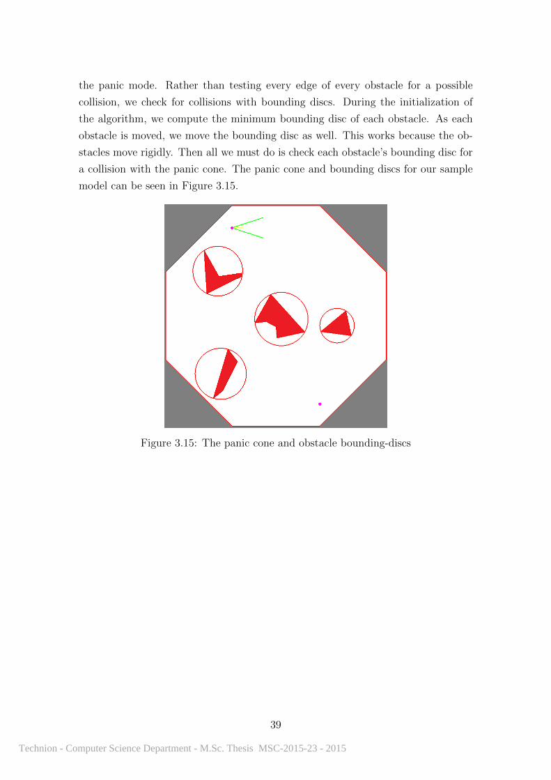
the panic mode. Rather than testing every edge of every obstacle for a possible

collision, we check for collisions with bounding discs. During the initialization of

the algorithm, we compute the minimum bounding disc of each obstacle. As each

obstacle is moved, we move the bounding disc as well. This works because the ob-

stacles move rigidly. Then all we must do is check each obstacle’s bounding disc for

a collision with the panic cone. The panic cone and bounding discs for our sample

model can be seen in Figure 3.15.

Figure 3.15: The panic cone and obstacle bounding-discs

39



Chapter 4

Curvature Augmentation Methods

We will now discuss three different possible methods of curvature augmentation.

For each method, we will show how we can compute the curve, how the curve

computation can fail, how we can test the maximum curvature, and how we can

compute the curve length. We will also show how the boundedness test can be

improved, so that a full point-crawl is not necessary.

1 Notation

We define the following:

P0, P1

The initial and final points of the curve,

v0, v1The unit vectors representing the initial and final orientations of the curve,

θ0, θ1The angle of the initial and final orientations of the curve, in radians,

κmaxThe maximum allowed curvature of the path,

FThe face spanned by the curve,

g0, g1 ∈ ∂FThe initial and final gates, by which the path enters F :P0 lies on g0 and P1 lies on g1, and

b0, b1 ∈ ∂FThe initial and final heading blocks.

41


2 Circle-to-Circle Spline

The first method we will discuss is called Circle-to-Circle (henceforth to be called

CtC Spline). In this method, we find a method that assumes either we are turning

at the maximum curvature, or else we are driving straight. To do this, we use the

initial point and orientation and the final point and orientation to each define a circle

of rotation, and the resulting path is an arc of the initial circle of rotation, followed

by a joint tangent, followed by an arc of the final circle of orientation. Examples

can be seen in Figure 4.1.

The idea of using sets of conic sections for interpolation, given interpolation

points and orientations, was introduced by R.A. Liming [19] for airplane design.

This method is still in use in a number of engineering disciplines, and opens a wide

array of possible curves. We use circles and lines because they are easy to manipulate

and create the shortest path.

Figure 4.1: Two CtC splines in the same scenario, with different maximum curva-tures

2.1 Computation

To compute the CtC spline, we begin by computing the two possible initial circles

of rotation. If we treat the initial point and vector as a tangent vector to a circle

of radius 1κmax

, we can compute the two centers by rotatating the initial vector by

±90°and translating from the initial point by the radius. We repeat this process

for the final vector, giving us two initial circles and two final circles, combining for

four pairs of circles. We then define the winding sign of the vector to be the sign

of rotation implied by the tangent vector (positive for counter-clockwise, negative

for clockwise). We compute the winding sign of the initial vector for each tangent

circle, and the winding sign of the final vector for each final tangent circle.

42


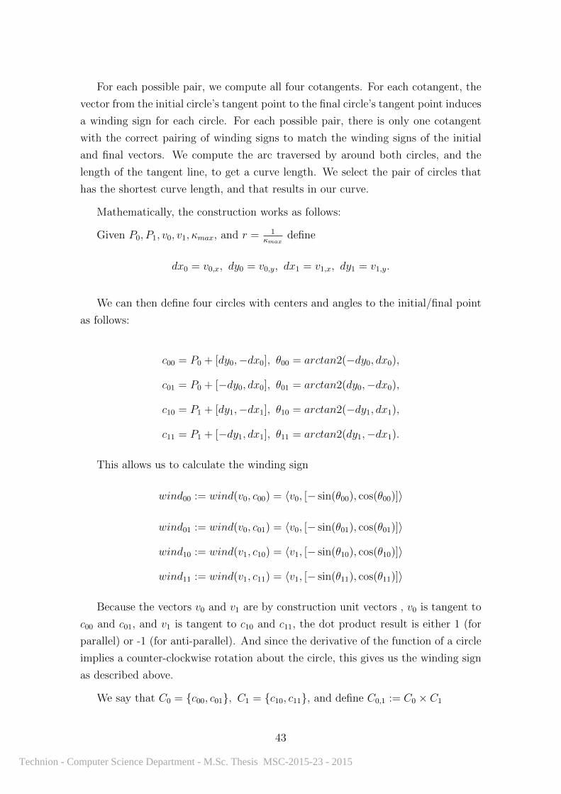
For each possible pair, we compute all four cotangents. For each cotangent, the

vector from the initial circle’s tangent point to the final circle’s tangent point induces

a winding sign for each circle. For each possible pair, there is only one cotangent

with the correct pairing of winding signs to match the winding signs of the initial

and final vectors. We compute the arc traversed by around both circles, and the

length of the tangent line, to get a curve length. We select the pair of circles that

has the shortest curve length, and that results in our curve.

Mathematically, the construction works as follows:

Given P0, P1, v0, v1, κmax, and r = 1κmax

define

dx0 = v0,x, dy0 = v0,y, dx1 = v1,x, dy1 = v1,y.

We can then define four circles with centers and angles to the initial/final point

as follows:

c00 = P0 + [dy0,−dx0], θ00 = arctan2(−dy0, dx0),

c01 = P0 + [−dy0, dx0], θ01 = arctan2(dy0,−dx0),

c10 = P1 + [dy1,−dx1], θ10 = arctan2(−dy1, dx1),

c11 = P1 + [−dy1, dx1], θ11 = arctan2(dy1,−dx1).

This allows us to calculate the winding sign

wind00 := wind(v0, c00) = 〈v0, [− sin(θ00), cos(θ00)]〉




Because the vectors v0 and v1 are by construction unit vectors , v0 is tangent to

c00 and c01, and v1 is tangent to c10 and c11, the dot product result is either 1 (for

parallel) or -1 (for anti-parallel). And since the derivative of the function of a circle

implies a counter-clockwise rotation about the circle, this gives us the winding sign

as described above.

We say that C0 = {c00, c01}, C1 = {c10, c11}, and define C0,1 := C0 × C1

43


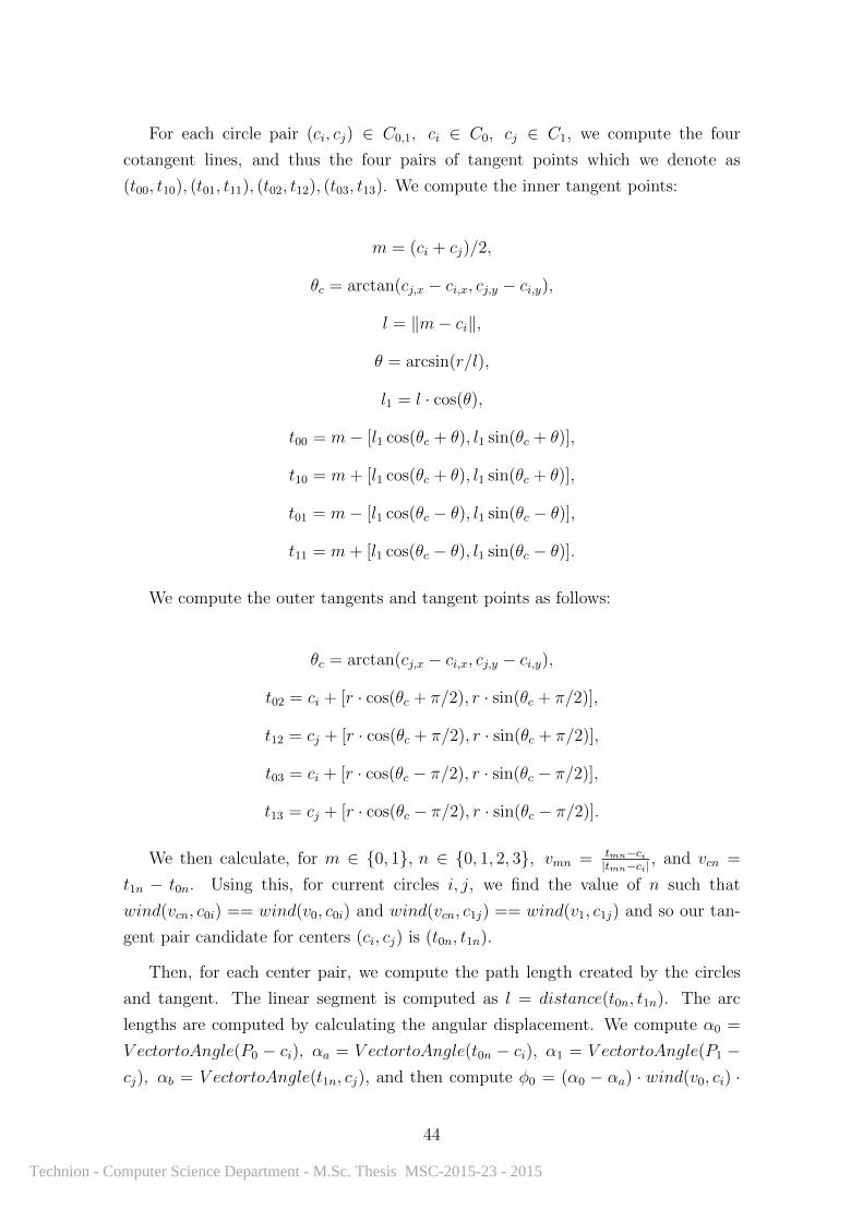
For each circle pair (ci, cj) ∈ C0,1, ci ∈ C0, cj ∈ C1, we compute the four

cotangent lines, and thus the four pairs of tangent points which we denote as

(t00, t10), (t01, t11), (t02, t12), (t03, t13). We compute the inner tangent points:

m = (ci + cj)/2,

θc = arctan(cj,x − ci,x, cj,y − ci,y),

l = ‖m− ci‖,

θ = arcsin(r/l),

l1 = l · cos(θ),

t00 = m− [l1 cos(θc + θ), l1 sin(θc + θ)],

t10 = m+ [l1 cos(θc + θ), l1 sin(θc + θ)],

t01 = m− [l1 cos(θc − θ), l1 sin(θc − θ)],

t11 = m+ [l1 cos(θc − θ), l1 sin(θc − θ)].

We compute the outer tangents and tangent points as follows:

θc = arctan(cj,x − ci,x, cj,y − ci,y),

t02 = ci + [r · cos(θc + π/2), r · sin(θc + π/2)],

t12 = cj + [r · cos(θc + π/2), r · sin(θc + π/2)],

t03 = ci + [r · cos(θc − π/2), r · sin(θc − π/2)],

t13 = cj + [r · cos(θc − π/2), r · sin(θc − π/2)].

We then calculate, for m ∈ {0, 1}, n ∈ {0, 1, 2, 3}, vmn = tmn−ci|tmn−ci| , and vcn =

t1n − t0n. Using this, for current circles i, j, we find the value of n such that

wind(vcn, c0i) == wind(v0, c0i) and wind(vcn, c1j) == wind(v1, c1j) and so our tan-

gent pair candidate for centers (ci, cj) is (t0n, t1n).

Then, for each center pair, we compute the path length created by the circles

and tangent. The linear segment is computed as l = distance(t0n, t1n). The arc

lengths are computed by calculating the angular displacement. We compute α0 =

V ectortoAngle(P0 − ci), αa = V ectortoAngle(t0n − ci), α1 = V ectortoAngle(P1 −cj), αb = V ectortoAngle(t1n, cj), and then compute φ0 = (α0 − αa) · wind(v0, ci) ·

44


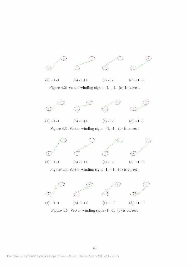
(a) +1 -1 (b) -1 +1 (c) -1 -1 (d) +1 +1

Figure 4.2: Vector winding signs +1, +1, (d) is correct

(a) +1 -1 (b) -1 +1 (c) -1 -1 (d) +1 +1

Figure 4.3: Vector winding signs +1, -1, (a) is correct

(a) +1 -1 (b) -1 +1 (c) -1 -1 (d) +1 +1

Figure 4.4: Vector winding signs -1, +1, (b) is correct

(a) +1 -1 (b) -1 +1 (c) -1 -1 (d) +1 +1

Figure 4.5: Vector winding signs -1, -1, (c) is correct

45


r, φ1 = (α1−αb) ·wind(v1, cj) · r. The curve length is computed as lij = l+φ0 +φ1.

We select the pair i, j that minimizes lij, and use that as our center pairing, with

the correct t0m, t1n.

Below we can see all possible circle pairs with all possible common tangent lines.

Figure 4.2 shows all common tangents for the scenario when both endpoints have

positive winding signs. In Figure 4.3, the point P0 has a positive winding sign while

P1 has a negative sign, and in Figure 4.4 we have the opposite case. Last, Figure

4.5 shows the scenario in which P0 and P1 have negative winding signs. Figure 4.6

shows the results of the first two iterations of our algorithm using CtC curves.

(a) The initial graph (b) The initial path (c) A tighter initialgraph

(d) A tighter initialpath

(e) The second itera-tion graph

(f) The second itera-tion path

(g) The tighter graph (h) The tighter path.

Figure 4.6: The resulting CtC spline graph and path for the first two iterationsof the algorithm (first iteration in the top row, second iteration in thebottom. The two leftmost columns are the result of a minimum radiusof curvature equal to five percent of the width of the workspace, and thetwo rightmost columns are the result of a minimum radius equal to 0.5percent of the width of the workspace.

2.2 Curve Length

The curve length is a direct result of the curve construction. The curve consists of

arcs of two circles with known radius, and a segment of the cotangent line that lies

between the two tangents. We sum the arc lengths and the line segment length to

get the curve length. We record this during the construction.

46


2.3 Maximum Curvature

The maximum curvature is also a direct result of the construction. The circular arcs

have curvature equal to the reciprocal of the radius, and the straight line segment

has a curvature of 0. Hence, the maximum curvature is equal to the curvature of

the arcs, and by construction the maximum curvature is the maximum curvature

allowed.

2.4 Failure of Computation

The computation fails if there are no matching pairs of circles with a joint tangent

such that the winding sign condition holds. However, this is not actually possible.

If there exists a pair of tangent circles that do not overlap at all, then all four joint

tangent lines must exist, and so there must be a winding sign match. Therefore, for

P0 we can select a tangent circle with center further from P1, and the reverse for P1,

resulting in two non-overlapping circles, so we must be able to find a match.

Numerically, if an end of the linear segment lies very close to an endpoint of the

segment, our computation can fail by determining that the tangent point is past

the endpoint, rather than before. Frequently, this can be solved by switching the

tangent circle being used, but not always, and so setting low values to zero gives a

fair approximation.

2.5 Improvements to the Boundedness Test

There are a number of ways we can accelerate the boundedness test. The first

method is to perform the point crawl from the beginning, just around the initial

arc, and to perform the crawl from the end, backwards around the final arc. If the

last point tested from both segments is within the bounds, then, since the bounding

face is convex, the entire linear segment is contained within the bounding face.

We can test a looser condition that will guarantee the curve is bounded, but is

more likely to fail. We can compute the intersection of the initial vector and the

tangent vector, and test if that point is bounded. We can also perform this for the

final point. If both points are bounded, then the entire curve is bounded. If either

point is not bounded, we can then use the point crawl on the correct end to test.

Clearly this will work better if the angle is smaller, but it can always be used to test

our results as long as neither circular arc is greater than or equal to 180°.

47


Another possible method is as follows. We begin by translating from the center

of the initial circle, along the initial orientation vector, until we reach the initial-

edge block. We may need to adjust the initial edge block, depending on the block’s

length and the location of the circle. We make sure the distance it is greater than the

radius of the circle. We repeat this process for the final circle. This will guarantee

that the middle line segment is completely bounded. We next ensure that the initial

and final arcs are bounded. Beginning at the initial edge, we find the edge’s second

intersection point with the initial circle. If that point is on the segment, the initial

arc is bounded if the point is further along the initial circle than the tangent point.

If the point is not on the segment, we move to the correct neighbor. We test the

intersections until we either pass the angle at which we exit the arc, or until we find

an intersection point. If we find the intersection point first, we are unbounded, but

if we find the exit angle, we are still bounded. We repeat this process for the end of

the curve by backtracking from the final point around the final circle until reaching

the point at which we exit the final arc. If we pass all four tests, the path is fully

bounded.

3 Cubic Bezier Spline

The next curve form we examine is that of cubic Bezier curves. A Bezier curve

is a parametric curve defined by Bezier [5] as follows: Given an ordered set of

n+ 1 control points, {P0, ..., Pn}, which is called the control polygon, we construct

a degree-n parametric polynomial γ(t) =n∑i=0

PiBi,n(t), where t ∈ [0, 1] and B(i, n)

is the Bernstein polynomial, which is defined [9] as Bi,n(t) =(ni

)ti(1 − t)n−i. The

equations for the curve and the first two derivatives are

γ(t) =3∑i=0

PiBi,n(t)

γ′(t) =n−1∑i=0

n(Pi+1 − Pi)Bn−1,i(t) and

γ′′(t) =n−2∑i=0

(n(n− 1))(Pi+2 − 2Pi+1 + Pi)Bn−2,i(t).

48


In the case of a cubic Bezier curve, we can rewrite these equations as

γ(t) = P0(1− t)3 + 3Pa(1− t)2t+ 3Pb(1− t)t2 + P1t3,

γ′(t) = 3(Pa − P0)(1− t)2 + 6(Pb − Pa)(1− t)t+ 3(P1 − Pb)t2

γ′′(t) = 6(Pb − 2Pa + P0)(1− t) + 6(P1 − 2Pb + Pa)t,

where the four control points are P0, Pa, Pb, and P1. Examples can be seen in Figure

4.7.

Bezier curves have a number of desirable properties that we can use to our advan-

tage. The first such property is the variation diminishing property [26]. According

to this property, the entire curve is contained within the convex hull of the control

points. The second property is that the curve interpolates the first and last control

points, and that the tangent at the endpoints is along the first and last edges of the

control polygon.

(a) A single Cubic Bezier Spline,with associated control polygon

(b) Two overlaid Cubic BezierSplines that differ by maximumcurvature

Figure 4.7: Examples of cubic Bezier curves

3.1 Computation

We wish to construct a cubic Bezier curve with maximum curvature equal to κmax.

The derivative of the curvature of a Bezier curve is a quintic function, and thus has

no analytic solutions. However, experimentally we see that the number of curvature

maxima of a Bezier curve is at most the number of turns in the control polygon, so

a cubic Bezier curve has at most two curvature maxima. Therefore, if the endpoint

curvature are local maxima, then the maximum curvature of the entire segment

is equal to the endpoint curvature. The construction of this curve attempts to

49


construct a curve whose endpoint curvature is equal to the maximum allowable

curvature.

Because we have fixed the first and last points, and we know the first and last

orientations, we simply need the length of the first and last segments of the control

polygon to get a curve with this property.

P0 is the initial point of the curve, P1 is the final point of the curve, v0 is the

initial unit vector, and v1 is the final unit vector. For simplicity of notation, we will

rotate v1 by 180°, so that the second interior control point lies a positive distance

along this vector from P1. Then, for some positive number α0, Pa := P0 + α0 · v0,and similarly for some positive number α1, we have Pb := P1 + α1 · v1. Therefore,

the goal is to compute α0 and α1.

Theorem 3.1. The lengths α0 and α1 for which κ(0) = ±κmax and κ(1) = ±κmaxare the real roots of the following quartic function:

27

8κ3maxα

40−S0 ·

9

2κ2max(v0×L)α2

0−S1 ·V 3α0+3

2κmax(v0×L)2−S1 ·(v1×L)V 2, (4.1)

and the associated value:

α1 =S0 · 32κmaxα

20 − v0 × L

V(4.2)

where S0 = sign(κ(0)) and S1 = sign(κ(1)).

Proof. The curvature of a planar parametric curve is defined as κ(γ(t)), which we

will write in shorthand as κ(t), such that κ(t) = γ′(t)×γ′′(t)‖γ′(t)‖3 .

By rearranging the derivatives of a cubic Bezier curve, we have

γ′(t) = 3(

(P1 − 3Pb + 3Pa − P0)t2 + 3(Pb − 2Pa + P0)t+ (Pa − P0)

),

γ′′(t) = 6(

(P1 − 3Pb + 3Pa − P0)t+ (Pb − 2Pa + P0)).

Furthermore, by assigning l0 := Pa − P0, l1 := Pb − Pa, l2 = P1 − Pb, we can

rewrite the above equations as

γ′(t) = 3(

(l2 − 2l1 + l0)t2 + 3(l1 − l0)t+ l0

)γ′′(t) = 6

((l2 − 2l1 + l0)t+ (l1 − l0)

)50


The first and second derivatives at the endpoints are:

γ′(0) = 3l0, γ′′(0) = 6(l1 − l0),γ′(1) = 3l2, γ′′(1) = 6(l2 − l0).

and therefore the curvature at the endpoints is

κ(0) =γ′(0)× γ′′(0)

‖γ′(0)‖3=

3l0 × 6(l1 − l0)‖3l0‖3

=2l0 × (l1 − l0)

3‖l0‖3=

2l0 × l13‖l0‖3

By a similar analysis we find that κ(1) = −2l2×l13‖l2‖3 . We then substitute:

l0 = Pa − P0 = P0 + α0v0 − P0 = α0v0,

l1 = Pb − Pa = P1 + α1v1 − P0 − α0v0,

l2 = P1 − Pb = P1 − P1 − α1v1 = −α1v1.

By defining L = P1 − P0 and V = v0 × v3, we can reformulate the endpoint

curvature as

κ(0) =2(α0v0 × (L+ α1v1 − α0v0)

3‖α0v0‖3=

2(v0 × L+ α1V )

3α20

(4.3)

κ(1) =−2(−α1v1 × (L+ α1v1 − α0v0)

3‖α1v1‖3=

2(v1 × L+ α0V )

3α21

(4.4)

We begin by assigning both endpoint curvatures to equal κmax.

κmax =2(v0 × L+ α1V )

3α20

α1 =32κmaxα

20 − v0 × LV

α21 =

94κ2maxα

40 − 3κmaxv0 × Lα2

0 + (v0 × L)2

V 2

κmax =2(v1 × L+ α0V )

3α21

α0 =32κmaxα

21 − v1 × LV

=278κ3maxα

40 − 9

2κ2max(v0 × L)α2

0 + 32κmax(v0 × L)2 − (v1 × L)V 2

V 3

(4.5)

51


By rearranging Equation 4.5, and applying the same process for the cases when

one or both endpoints have negative curvature, we find Equations (4.1) and (4.2). �

We also need to consider the case where the curve has no curvature at one of the

endpoints (κ(0) = 0 or κ(1) = 0).

Corollary 3.1.1. The lengths α0 and α1 for which κ(0) = ±κmax and κ(1) = 0 are

α0 =−v1 × L

V(4.6)

α1 =±3

2κmaxα

20 − v0 × LV

(4.7)

Similarly, the lengths for which κ(0) = 0 and κ(1) = ±κmax are

α1 =−v0 × L

V(4.8)

α0 =±3

2κmaxα

21 − v1 × LV

(4.9)

where S0 = sign(κ(0)) and S1 = sign(κ(1)).

Proof. This is a direct result of Equations (4.3) and (4.4). �

We can now compute the interim points that would result in a correct endpoint

curvature. We must examine a number of separate cases.

In the general case, in which no two of the three line segments are parallel or

anti-parallel, we solve for the two lengths by first assigning the endpoint absolute

curvatures to equal κmax. We can then find the solutions by solving Equations

(4.1) and (4.2). By considering all four possible cases of the sign of the endpoint

curvature, we get four quartic functions and 16 possible values for α0, and associated

α1 values. This results in 16 pairs, {(α0,0, α1,0), ..., (α0,15, α1,15)}.

We must also consider the case where only one endpoint curvature is equal to

κmax, and the other endpoint curvature is equal to 0. This occurs when the result

of the computation is such that the first interim point is on the line passing through

P1 with orientation v1, or the second interim point is on the line passing through

P0 with orientation v0. By solving Equations (4.6) and (4.7), as well as solving

Equations (4.8) and (4.9), we find another four possible solutions, giving us a total

of 20 solution pairs.

52


We take all results in which both values are positive and real, and compute

the resulting middle segment length, l2,i = L + α3,iv3 − α0,iv0. We finally compute

Di = α0,i + li + α3,i and find min(Di), which selects the shortest control polygon

and gives us our resulting interim points.

There are a 2 special cases that need to be considered separately.

1. v0 × v1 ≈ 0, v0 × L ≈ 0, v1 × L ≈ 0

This is the fully degenerate case, where all three line segments are parallel, and

therefore all four points of the control polygon are colinear. In this case, it is trivial

to see that κ(0) = κ(1) = 0. Hence, we may select arbitrary lengths, for which we

will use α0 = α1 = ‖L‖3

.

2. v0 × v3 ≈ 0, v0 × L 6≈ 0, v3 × L 6≈ 0

In this case, the initial and final headings (and therefore the outer line segments)

are parallel, but the middle line segment is not parallel to the outer line segments.

In this case, the equations simplify to independent functions as follows.

κ(0) =2(v0 × L)

3α20

κ(1) =2(v3 × L)

3α23

We can then solve for the lengths by computing α0 =√

2|v0×L|3κmax

and α3 =√2|v3×L|3κmax

.

Figure 4.8 shows the results of the first two iterations of our algorithm using

cubic Bezier curve segments.

3.2 Curve Length

The exact length of a Bezier curve is not computable analytically. However, the

length of a Bezier curve is bounded from above by the length of the control poly-

gon [4]. Therefore, we can use the control polygon’s length as an approximation.

This length is a direct result of the construction of the curve.

53


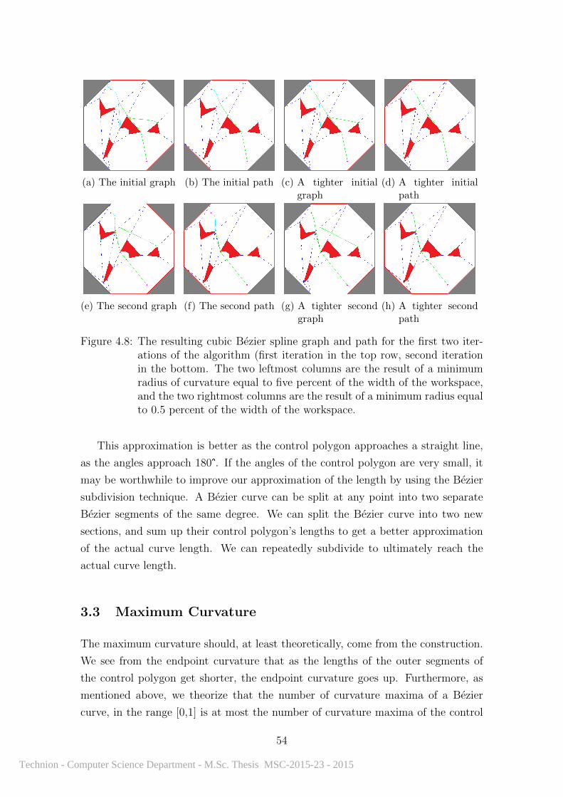
(a) The initial graph (b) The initial path (c) A tighter initialgraph

(d) A tighter initialpath

(e) The second graph (f) The second path (g) A tighter secondgraph

(h) A tighter secondpath

Figure 4.8: The resulting cubic Bezier spline graph and path for the first two iter-ations of the algorithm (first iteration in the top row, second iterationin the bottom. The two leftmost columns are the result of a minimumradius of curvature equal to five percent of the width of the workspace,and the two rightmost columns are the result of a minimum radius equalto 0.5 percent of the width of the workspace.

This approximation is better as the control polygon approaches a straight line,

as the angles approach 180°. If the angles of the control polygon are very small, it

may be worthwhile to improve our approximation of the length by using the Bezier

subdivision technique. A Bezier curve can be split at any point into two separate

Bezier segments of the same degree. We can split the Bezier curve into two new

sections, and sum up their control polygon’s lengths to get a better approximation

of the actual curve length. We can repeatedly subdivide to ultimately reach the

actual curve length.


The maximum curvature should, at least theoretically, come from the construction.

We see from the endpoint curvature that as the lengths of the outer segments of

the control polygon get shorter, the endpoint curvature goes up. Furthermore, as

mentioned above, we theorize that the number of curvature maxima of a Bezier

curve, in the range [0,1] is at most the number of curvature maxima of the control

54


polygon (in the case of a cubic, this is two). Therefore, we test the curvature

slightly off the endpoints to see if the curvature is absolutely less than the endpoint

curvatures. If we are still concerned about a sharp peak, we can also compute the

derivative of the curvature both at and near the endpoints to make sure that we did

not miss a local maximum.

This, however, is not an absolute proof of the maximum curvature. The deriva-

tive of the curvature is a quintic function with respect to t, and therefore has no

analytic solution, so we cannot know for certain how many curvature maxima there

are in the range of [0,1]. However, experimentally our theorem does hold true, espe-

cially as the outer segments of the control polygon get shorter relative to the middle

segment, and so we will rely on it to get an approximation.

One can also use a numerical root finder to try to find roots for the curvature, and

test where the maxima are, and check if these maxima are less than the maximum

allowed curvature. This is safer, but experimentally not necessary.


Theoretically, the general case computation fails when the control polygon contains

two or more parallel line segments. If l0||l1 or l2||l1 then there is only one curvature

maximum, and the appropriate endpoint has curvature 0. Furthermore, if all three

line segments are parallel, then the entire line segment has curvature 0. Numerically,

there are also have issues when l0||l2. By including the special cases mentioned above,

solutions are available as long as P0 is not in the same location as P1.

In all these cases, there may be no actual solution, which would mean that all

solution pairs contain either a non-real or non-positive value. This is easily detected

during the computation.

3.5 Improvements of the Boundedness Test

The boundedness test becomes very simple. One well known property of Bezier

curves is the variation diminishing property, which states that no line can pass

through the Bezier curve more times than it passes through the control polygon [10].

This means that any edge of the bounding face cannot pass through the curve

without passing through the control polygon. Thus, if the control polygon is fully

contained within the face, then the entire curve is contained. All we need to do is

show that the two interim control points on the curve are within the face and we

55


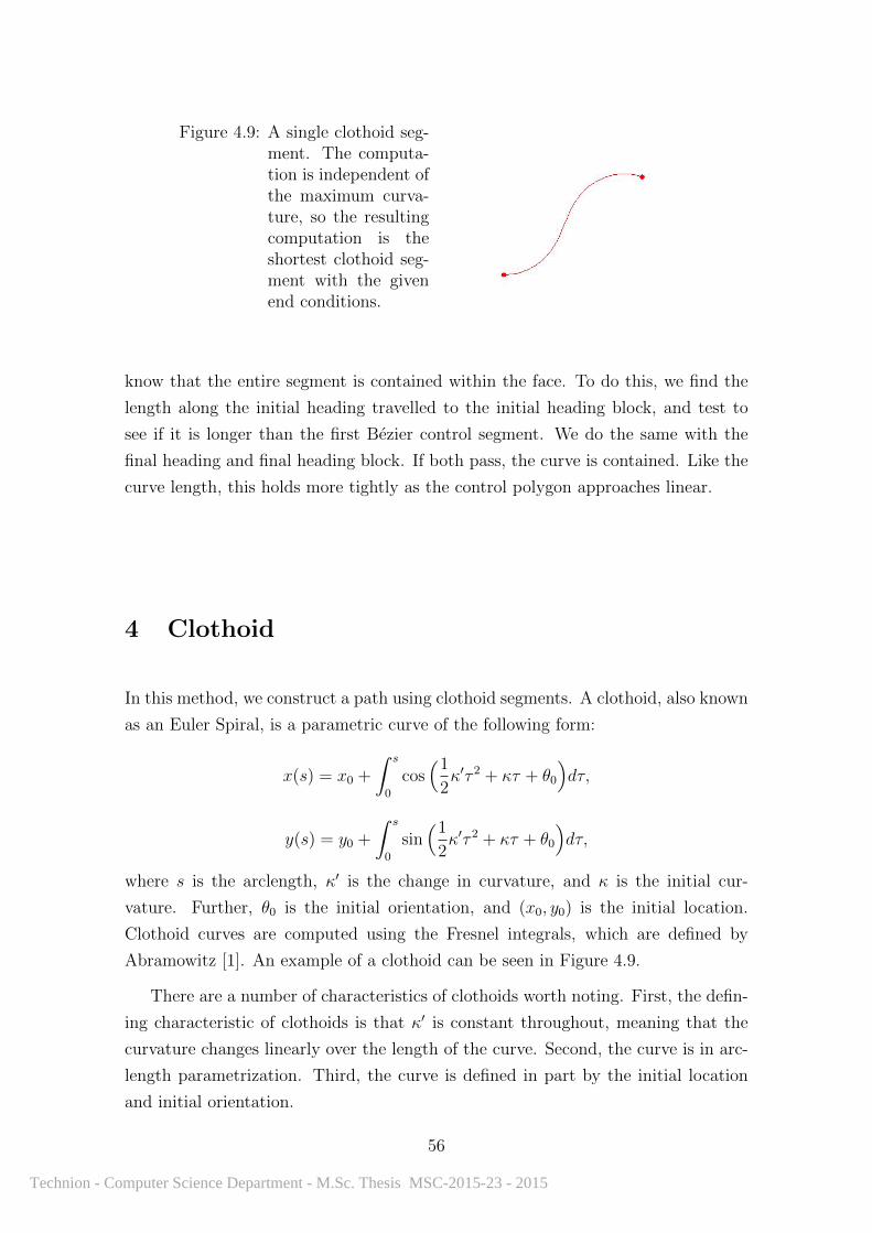
Figure 4.9: A single clothoid seg-ment. The computa-tion is independent ofthe maximum curva-ture, so the resultingcomputation is theshortest clothoid seg-ment with the givenend conditions.

know that the entire segment is contained within the face. To do this, we find the

length along the initial heading travelled to the initial heading block, and test to

see if it is longer than the first Bezier control segment. We do the same with the

final heading and final heading block. If both pass, the curve is contained. Like the

curve length, this holds more tightly as the control polygon approaches linear.

4 Clothoid

In this method, we construct a path using clothoid segments. A clothoid, also known

as an Euler Spiral, is a parametric curve of the following form:

x(s) = x0 +

∫ s

0

cos(1

2κ′τ 2 + κτ + θ0

)dτ,

y(s) = y0 +

∫ s

0

sin(1

2κ′τ 2 + κτ + θ0

)dτ,

where s is the arclength, κ′ is the change in curvature, and κ is the initial cur-

vature. Further, θ0 is the initial orientation, and (x0, y0) is the initial location.

Clothoid curves are computed using the Fresnel integrals, which are defined by

Abramowitz [1]. An example of a clothoid can be seen in Figure 4.9.

There are a number of characteristics of clothoids worth noting. First, the defin-

ing characteristic of clothoids is that κ′ is constant throughout, meaning that the

curvature changes linearly over the length of the curve. Second, the curve is in arc-

length parametrization. Third, the curve is defined in part by the initial location

and initial orientation.

56


4.1 Computation

We will use the derivation presented by Bertolazzi and Frego [3] to find the minimum

length clothoid from an initial point and initial orientation to a final point and final

orientation. Specifically, the problem they try to solve is to find the minimum

positive value L such that x(0) = x0, y(0) = y0, arctan(y′(0)x′(0)

)= θ0, x(L) =

x1, y(L) = y1, arctan(y′(L)x′(L)

)= θ1, identical to the problem we are trying to solve.

The method works as follows. The algorithm is searching for the zero of the

following system of nonlinear equations:

F(L, κ, κ′) =

x1 − x0 −∫ L0

cos(12κ′s2 + κs+ θ0)ds

y1 − y0 −∫ L0

sin(12κ′s2 + κs+ θ0)ds

θ1 − (12κ′L+ κL+ θ0)

.

By assigning A = 12κ′L2, B = Lκ, ∆x = x1 − x0, and ∆y = y1 − y0, we can

reformulate this to

F(L,B

L,2A

L2) =

∆x− L∫ 1

0cos(Aτ 2 +Bτ + θ0)dτ

∆y − L∫ 1

0sin(Aτ 2 +Bτ + θ0)dτ

θ1 − (A+B + θ0)

.

Since the third equation is linear, we can solve it with respect to B, B = ∆θ−A,∆θ = θ1 − θ0, so we reduce the system of nonlinear equations to two equations in

two unknowns:

G(L,A) =

(∆x− L

∫ 1

0cos(Aτ 2 + (∆θ − A)τ + θ0)dτ

∆y − L∫ 1

0sin(Aτ 2 + (∆θ − A)τ + θ0)dτ

).

By representing in polar coordinates, ∆x = r ·cosφ, ∆y = r ·sinφ, we can define

two new functions

f(L,A) = G(L,A) ·

(cosφ

sinφ

), and g(A) =

1

LG(L,A) ·

(cosφ

sinφ

).

57


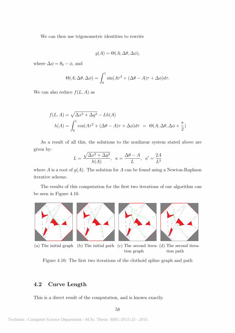
We can then use trigonometric identities to rewrite

g(A) = Θ(A; ∆θ,∆φ),

where ∆φ = θ0 − φ, and

Θ(A; ∆θ,∆φ) =

∫ 1

0

sin(Aτ 2 + (∆θ − A)τ + ∆φ)dτ.

We can also reduce f(L,A) as

f(L,A) =√

∆x2 + ∆y2 − Lh(A)

h(A) =

∫ 1

0

cos(Aτ 2 + (∆θ − A)τ + ∆φ)dτ = Θ(A; ∆θ,∆φ+π

2)

As a result of all this, the solutions to the nonlinear system stated above are

given by:

L =

√∆x2 + ∆y2

h(A), κ =

∆θ − AL

, κ′ =2A

L2

where A is a root of g(A). The solution for A can be found using a Newton-Raphson

iterative scheme.

The results of this computation for the first two iterations of our algorithm can

be seen in Figure 4.10.

(a) The initial graph (b) The initial path (c) The second itera-tion graph

(d) The second itera-tion path

Figure 4.10: The first two iterations of the clothoid spline graph and path

4.2 Curve Length

This is a direct result of the computation, and is known exactly.

58



This is also a direct result of the computation. It is the greater of |κ0| and |κ0+L·κ′|.


The algorithm will return a negative length if the computation fails. This occurs

when the entire segment is linear.

4.5 Improvements of the Boundedness Test

Because of the form of the curve, there is no real improvements that can be made.

59



Chapter 5

Analysis of the Algorithm

1 Correctness and Completeness

For the most part, it is trivial to show that the algorithm is both correct and

complete. The fusion of two convex regions, the construction and maintenance of

the search graph, and the initial path approximation do not require clarification. The

path-augmentation methods have all been shown already. There are a few portions

of the algorithm that are not so simple, and here we explain those portions.

1.1 Finding an Axis of Monotonicity

Preparata and Supowit [24] proved the correctness of this algorithm on a single face.

From the definition of monotonicity, we know that a vertex that is convex in the

polygon will not affect monotonicity, so we restrict our search to concave vertices.

Furthermore, the definition also tells us that any straight line perpendicular to the

axis of monotonicity intersects the polygon at most twice, so for two adjacent edges

that meet at a concave vertex, a straight line can only pass through at most one

of the two edges. Any line that passes through the vertex, and is between the two

edges, has a slope such that any line parallel to it will intersect at most one of the

two edges. Therefore, any such line can be perpendicular to an axis of monotonocity.

This creates a closed range of possible slopes for the axis of monotonicity. A scan

of all vertices of the polygon finds all such ranges. As described above, we can use

these ranges to determine if an axis exists, and if so what it is. The algorithm used

has been proven correct, and so this algorithm is correct. This algorithm is also

complete in that every single vertex is tested, and so every range of slopes is found.

61


1.2 Concave clipping

Theorem 1.1. The concave clipping algorithm described above is correct and com-

plete.

Proof. In the case of a non-monotone polygon, all of our options have already been

proven to be complete and correct. Every simple polygon has diagonals, can be

triangulated, and can be decomposed into monotone regions. These are all well

known algorithms, and can be found elsewhere [2].

The monotone-decomposition algorithm is correct and complete, as a variant

of the traditional algorithm. The algorithm in the literature is designed to fully

triangulate the polygon, while our variant separates a monotone polygon into convex

regions but skips adding unnecessary edges. We assume that the polygon is x -

monotone, and we begin at the leftmost vertex. Because the polygon is x -monotone,

this vertex is guaranteed to be convex. As we advance each iterator, if we reach a

convex vertex, then no new gate is necessary. Each previously-visited vertex is

convex, and so the new gate would be splitting two convex vertices, and would be

removed immediately.

Once a concave vertex is reached, we have two case; either the two vertices are

not adjacent or they are. The difference between the two cases is that in the first

case a diagonal can be added to the polygon, and in the second no diagonal can

be added because the diagonal would be the boundary edge or a previously-added

diagonal. In the first case, since we have not reached our stopping condition on

the second iterator, we can add a diagonal to the polygon connecting the concave

vertex to the second iterator’s vertex, and create a convex angle to the left of the

added diagonal. Once this occurs, any of the other potential diagonals would again

be splitting two convex vertices and as such is not necessary. However, if we have

not yet reached the stopping condition, that means that a later diagonal would

create a convex vertex to the left of the diagonal, and adding a diagonal now would

retroactively split two convex vertices, and would ultimately become unnecessary.

In the second case, because no new diagonal can be added using our method,

we use the standard triangulation algorithm, which is correct and complete. If we

reach a point when the stack consists of two adjacent convex vertices (and no other

vertices), then we can begin our algorithm again. �

62


1.3 Path Creation and Updates

It is trivial to see that the initial path finding is correct and complete. If there

is a path from the robot to target, then by the correctness of the decomposition

algorithm there is a sequence of convex regions that leads from the robot to the

target. Therefore, there must be a sequence of gates that separate the regions, and

thus a sequence of nodes in the graph connected by edges that lead from the robot

to the target.

Theorem 1.2. Under the update process we apply to the linear path, the complete

path length always tends towards a local minimum.

Proof. It is trivial to see that the passthrough function finds the shortest path

between two points that passes through a gate.

The length of the underlying linear path is equal to the sum of the path lengths.

During each iteration we pass over the entire path, and perform an update operation

on each node in the path. If the node’s location is either already at the passthrough

point, in which case no local improvement can be made to the path, or else the

node’s location is not at the passthrough point, in which case moving the node’s

location will shorten this portion of the path, thus shortening the entire length of

the path. Therefore, we have a monotone decreasing function, which is certainly

bounded from below, so the total path length always converges to some value. �

In practice, the convergence is very fast, and the limit indeed appears to be the

best possible (smallest) path length, or a very good approximation thereof.

2 Complexity

Let us denote by n the complexity of the model, the total number of vertices of the

workspace and the obstacles. Formally, n := |W |+b∑i=0

|Bi| (since each obstacle moves

rigidly, its complexity does not change over time, so we ignore the time parameter).

The space complexity of the entire algorithm is O(n). The DCEL structure used

for the convex decomposition requires storing the vertices, edges, and faces. Since

the graph is planar, the size of all these lists are linearly related. Similarly, because

we prune the search graph, the size of the search graph is a linear function of n, and

so the entire space requirement is linear with respect to n.

63


Before discussing runtime complexity, we begin with a lemma to help our anal-

ysis.

Lemma 2.1. If an operation can be performed on a single face of the convex decom-

position in time linear with the complexity of the face, then the same operation can

be performed on all faces in the convex decomposition in time linear with respect to

the complexity of the entire model.

Proof. The claim follows immediately from the fact that the convex decomposition

is a planar graph, and hence its complexity is of the same order as the sum of

complexities of the individual faces. (Some multiplicative constant may be involved

since every edge is shared by one or two faces, and since in a planar graph, the

numbers of vertices, edges, and faces are all linear with each other.) �

2.1 Convex Decomposition

Maintaining the convex decomposition consists of testing each face for convexity,

finding an axis of monotonicity for each concave face (if any axis exists), and re-

moving any gates that split two convex vertices. It is important to mention that

because the obstacles cannot intersect, and because the gates cannot intersect, the

entire model is always planar. This is important, because the number of edges and

faces of a planar graph are known to be a linear function of the number of ver-

tices. Testing each face for convexity is a linear-time operation with respect to the

complexity of the face. This means that we must visit each bounding halfedge O(1)

times, and so testing the entire model means visiting each halfedge twice that, which

results in a complexity of O(n) over the entire model.

Theorem 2.2. Finding axes of monotonicity for all faces is the decomposition is

an O(n)-time algorithm.

Proof. Preparata and Supowit [24] prove that an axis of monotonicity can be found

in optimally linear time using a sequential algorithm. We previously described the

algorithm in Section 4.2, and showed an implementation in Figure 3.4. Therefore,

by Lemma 2.1, we know that all faces can be processed in O(n)-time. �

We can also apply similar logic to removing unnecessary edges. Each gate must

be visited once, and requires a constant-time operation to skip or remove. Since

there are a linear number of gates (with respect to n), this step also has a runtime

complexity of O(n).

64


Decomposing monotone regions, given the axis of monotonicity, is a linear time

algorithm, as shown above. While processing each face, we visit each bounding

halfedge once, and so overall we visit each edge at most twice, meaning the entire

algorithm runs in O(n) time. Decomposing non-monotone regions is theoretically a

linear time algorithm, because we can theoretically triangulate the polygon in linear

time [8]. However, as we are not aware at this point of any successful implementa-

tion of Chazelle’s algorithm, we must use one of our other methods. Performing a

monotone decomposition is known to be an O(n log n)-time algorithm.

As a result of all this, maintaining the convex decomposition takes theoreti-

cally O(n) time. In reality, the algorithm requires O(n)-time test if all faces of the

decomposition are monotone. If they all are monotone, then maintaining the decom-

position takes O(n) time; otherwise, maintaining the decomposition takes O(n log n)

time.

2.2 Search Graph Construction and Maintenance

Constructing a single node of the graph is a constant-time operation. We already

have the nodes and just need to compute the endpoint, which is a constant-time

operation. Similarly, updating the endpoints of a single node requires constant time,

because we just need to perform a constant-time operation to compute the initial

point.

If a node was removed due to the child’s exit gate being removed, merging the

list of children into the parent’s list of children can be done in constant time. This

can be done by storing the children as a linked list, along with pointers to the first

and last elements of the linked list.

Last, if a gate was added to the tree, we need to insert nodes into the search

graph and split edges. This can be done in O(n) time over the entire graph.

Theorem 2.3. All nodes can be inserted into the search graph, and the correct

updates made to the edges, in time linear with respect to the size of the entire search

graph.

Proof. We present a proof by construction.

For an edge of the search graph, e, splitting e.children can be done in time linear

with respect to the size of e.children, as follows.

65


By construction, for a search graph edge e, the edges in e.children are ordered

such that their end node edges are ordered counter-clockwise about the adjacent face

of e.end.g.twin, which we will call the output face. As we construct the children, we

create the edges as we iterate about the output face, and thus the initially created

children are in counter-clockwise order. When a node is removed, the outgoing edges

are already in counter-clockwise order, and by using the above process the ordering

can be maintained.

Furthermore, we allow each gate in the model to maintain a pointer to the

incoming edge of the search edge, and a record of whether the gate was created this

iteration or in an previous iteration. Since we prune the tree, and don’t allow two

incoming edges of the search graph to the same gate, we only need to maintain one

incoming edge, and it can be updated very simply in constant time.

To insert a node, and then split e.children correctly, we begin by maintaining a

new list to the side, unseen, which begins initialized to e.children, in order. We also

maintain a stack of added gates that we reach added (initialized to empty), and a

pointer to a current edge c (initialized to e). We begin by iterating counter-clockwise

about the output face of c, checking each bounding edge f to see if f is

� An old gate,

� A new gate, or

� c.end.g.twin.

If f is an old gate, then we check if f ’s incoming search-graph edge is the head

of unseen; if yes, then we remove the head of unseen, and add it to the end of

c.children.

If f is a new gate, then we create a new node, and a new incoming edge, c′. We

set c′.parent := c, and add c′ to the end of c.children. We then push c onto added,

and set c to point at c′.

Last, if f is the twin of c’s ending edge, then we set c := added.pop.

We continue this process until we attempt to pop from added when added is

empty, meaning we have reached the twin of e’s ending edge. Once this whole process

has been completed, every children list is still ordered correctly, by construction, and

each list of children contains the correct set of children (as can be trivially seen).

Because we prune the tree, as mentioned above, each gate halfedge can have only

one incoming search graph edge, meaning that any face of the convex decomposition

66


can only be the bounding face of the children of one edge of the search graph.

This means that each halfedge is visited at most once, and so the entire process is

completed in O(n) time. �

Since each of the above components is a linear-time operation, the entire main-

tenance of the search graph is a linear-time algorithm.

2.3 Path Augmentation

As can be seen above, augmenting each section of the path is a constant-time oper-

ation, as is testing the curvature of each section, and testing to see if the section is

bound to the correct face. However, finding the heading blocks is not linear. While

we can try to speed up the process as much as possible, and usually we can maintain

the same heading block from iteration to iteration, this process is an O(n2)-time op-

eration, because for each gate we must check every edge on the boundary of the

bounding face.

2.4 Total Complexity

As can be seen above, the convex decomposition requires linear time to test if the

all regions are convex or monotone, and at worst O(n log n)-time to maintain the

convexity. However, we only must use the more complex decomposition method

in cases of non-monotone polygons. As we will see in Sec.2.1, most regions are

monotone. Therefore, most iterations can be completed in linear time, and even

in situations where we must use the more complex decomposition, we only must

use the non-monotone decomposition for a few faces, rather than for the entire

decomposition.

Maintaining the optimality of the convex decomposition, fusing the regions into

larger convex regions, can be completed in linear time, as can maintaining the

search graph. Therefore, we can compute and maintain a piecewise-linear path

in O(n log n)-time in the worst case, but usually in O(n)-time.

The final portion of the algorithm, augmenting the path, is an O(n2)-time opera-

tion, due to the heading blocks. However, the heading blocks must only be changed

in two cases. The first is when the bounding face has transformed sufficiently over

time to change the heading block; because of the smoothness of the obstacle mo-

tion, this does not happen too frequently. The second case when we must change

67


the heading block is when one of the heading blocks gets removed due to the main-

tenance of the convex decomposition. As we see in Sec.2.1, this does not happen

to frequently, and then only to a small number of regions. Therefore, while the

complexity bound is correct, it is generally far beyond the observed runtime.

68


Chapter 6

Results

We present results to show the performance of the algorithm. To test the algo-

rithm, we randomly generated 470 scenarios with a polygonal workspace, polygonal

obstacles, and a starting point and target point in the initial freespace.

1 Implementation

We implemented the algorithm in C++, using the Microsoft Foundation Class

(MFC) libraries for the user interface. The inputs for the system are configura-

tion files that contain the model information. The files list the number of obstacles,

followed by the complexity of the workspace, and then the vertices of the workspace

in counter-clockwise order. Next, for each obstacle, the file lists the complexity of

the obstacle, followed by the vertices of the obstacle listed in counter-clockwise or-

der. Last, we list the source point and target point. Each item is listed individually

on a line. Figure 6.1 shows the configuration file for a sample model.

The system contains three main modules. There is a navigator, in charge of

running the algorithm described in this thesis. Second, there is a set of mobile ob-

stacles. Last, there is a manager to oversee the entire process. The primary purpose

of the manager is to maintain consistency between the vertices of the obstacles and

workspace, and the vertices the navigator uses. During each iteration of the algo-

rithm, the manager synchronizes the vertices, then signals the navigator to update

the navigation. The navigation manager also maintains various structures for test-

ing and debugging purposes, such as the visibility graph, so that we can compare

our results to the shortest path.

69


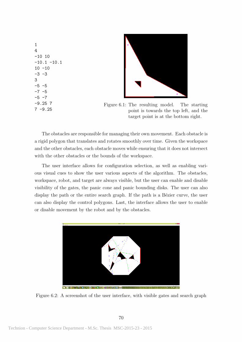
1

4

-10 10

-10.1 -10.1

10 -10

-3 -3

3

-5 -5

-7 -5

-5 -7

-9.25 7

7 -9.25Figure 6.1: The resulting model. The starting

point is towards the top left, and thetarget point is at the bottom right.

The obstacles are responsible for managing their own movement. Each obstacle is

a rigid polygon that translates and rotates smoothly over time. Given the workspace

and the other obstacles, each obstacle moves while ensuring that it does not intersect

with the other obstacles or the bounds of the workspace.

The user interface allows for configuration selection, as well as enabling vari-

ous visual cues to show the user various aspects of the algorithm. The obstacles,

workspace, robot, and target are always visible, but the user can enable and disable

visibility of the gates, the panic cone and panic bounding disks. The user can also

display the path or the entire search graph. If the path is a Bezier curve, the user

can also display the control polygons. Last, the interface allows the user to enable

or disable movement by the robot and by the obstacles.

Figure 6.2: A screenshot of the user interface, with visible gates and search graph

70


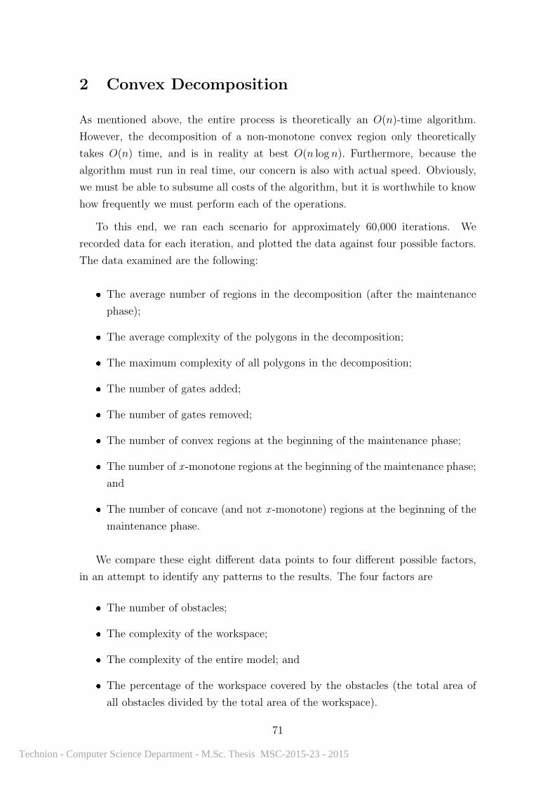
2 Convex Decomposition

As mentioned above, the entire process is theoretically an O(n)-time algorithm.

However, the decomposition of a non-monotone convex region only theoretically

takes O(n) time, and is in reality at best O(n log n). Furthermore, because the

algorithm must run in real time, our concern is also with actual speed. Obviously,

we must be able to subsume all costs of the algorithm, but it is worthwhile to know

how frequently we must perform each of the operations.

To this end, we ran each scenario for approximately 60,000 iterations. We

recorded data for each iteration, and plotted the data against four possible factors.

The data examined are the following:

� The average number of regions in the decomposition (after the maintenance

phase);

� The average complexity of the polygons in the decomposition;

� The maximum complexity of all polygons in the decomposition;

� The number of gates added;

� The number of gates removed;

� The number of convex regions at the beginning of the maintenance phase;

� The number of x -monotone regions at the beginning of the maintenance phase;

and

� The number of concave (and not x -monotone) regions at the beginning of the

maintenance phase.

We compare these eight different data points to four different possible factors,

in an attempt to identify any patterns to the results. The four factors are

� The number of obstacles;

� The complexity of the workspace;

� The complexity of the entire model; and

� The percentage of the workspace covered by the obstacles (the total area of

all obstacles divided by the total area of the workspace).

71


For simplicity, in each set of graphs, we plot against the four different factors in the

order listed above, going left to right; the x-axis of the leftmost graph is the number

of obstacles, followed by the complexity of the workspace, and so on.

2.1 Average Numbers of Polygonal Regions

Figure 6.3: The number of polygons in the decomposition

Figure 6.4: The number of convex polygons, before the maintenance stage

Figures 6.3 through 6.6 show that the number of regions is clearly a linear func-

tion of both the number of obstacles and of the complexity of the entire model. There

also appears to be a weaker correlation between the order of the workspace and the

number of regions, as well as between the percentage of the workspace covered by

obstacles (the ratio of the total area of the obstacles to the area of the workspace).

In both of these datasets, the minimum average number of regions stayed fairly

constant while the maximum observed averages rose with the independent variable.

Next, we examine the number of convex, monotone, and concave regions in

the decomposition after the obstacles have moved, but before the convexity has

been maintained (at the beginning of each iteration of the algorithm). We see that

Figure 6.5: The number of monotone polygons, before the maintenance stage

72


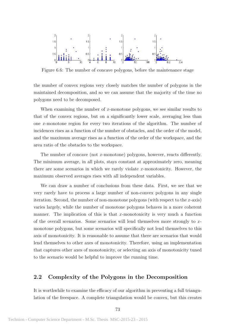
Figure 6.6: The number of concave polygons, before the maintenance stage

the number of convex regions very closely matches the number of polygons in the

maintained decomposition, and so we can assume that the majority of the time no

polygons need to be decomposed.

When examining the number of x -monotone polygons, we see similar results to

that of the convex regions, but on a significantly lower scale, averaging less than

one x -monotone region for every two iterations of the algorithm. The number of

incidences rises as a function of the number of obstacles, and the order of the model,

and the maximum average rises as a function of the order of the workspace, and the

area ratio of the obstacles to the workspace.

The number of concave (not x -monotone) polygons, however, reacts differently.

The minimum average, in all plots, stays constant at approximately zero, meaning

there are some scenarios in which we rarely violate x -monotonicity. However, the

maximum observed averages rises with all independent variables.

We can draw a number of conclusions from these data. First, we see that we

very rarely have to process a large number of non-convex polygons in any single

iteration. Second, the number of non-monotone polygons (with respect to the x -axis)

varies largely, while the number of monotone polygons behaves in a more coherent

manner. The implication of this is that x -monotonicity is very much a function

of the overall scenarios. Some scenarios will lend themselves more strongly to x -

monotone polygons, but some scenarios will specifically not lend themselves to this

axis of monotonicity. It is reasonable to assume that there are scenarios that would

lend themselves to other axes of monotonicity. Therefore, using an implementation

that captures other axes of monotonicity, or selecting an axis of monotonicity tuned

to the scenario would be helpful to improve the running time.

2.2 Complexity of the Polygons in the Decomposition

It is worthwhile to examine the efficacy of our algorithm in preventing a full triangu-

lation of the freespace. A complete triangulation would be convex, but this creates

73


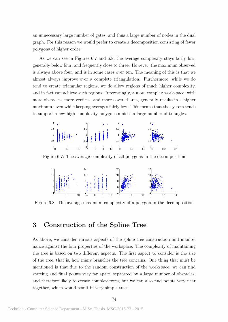
an unnecessary large number of gates, and thus a large number of nodes in the dual

graph. For this reason we would prefer to create a decomposition consisting of fewer

polygons of higher order.

As we can see in Figures 6.7 and 6.8, the average complexity stays fairly low,

generally below four, and frequently close to three. However, the maximum observed

is always above four, and is in some cases over ten. The meaning of this is that we

almost always improve over a complete triangulation. Furthermore, while we do

tend to create triangular regions, we do allow regions of much higher complexity,

and in fact can achieve such regions. Interestingly, a more complex workspace, with

more obstacles, more vertices, and more covered area, generally results in a higher

maximum, even while keeping averages fairly low. This means that the system tends

to support a few high-complexity polygons amidst a large number of triangles.

Figure 6.7: The average complexity of all polygons in the decomposition

Figure 6.8: The average maximum complexity of a polygon in the decomposition

3 Construction of the Spline Tree

As above, we consider various aspects of the spline tree construction and mainte-

nance against the four properties of the workspace. The complexity of maintaining

the tree is based on two different aspects. The first aspect to consider is the size

of the tree, that is, how many branches the tree contains. One thing that must be

mentioned is that due to the random construction of the workspace, we can find

starting and final points very far apart, separated by a large number of obstacles,

and therefore likely to create complex trees, but we can also find points very near

together, which would result in very simple trees.

74


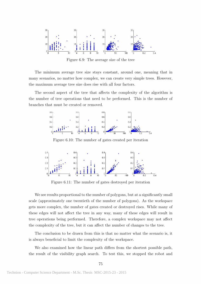
Figure 6.9: The average size of the tree

The minimum average tree size stays constant, around one, meaning that in

many scenarios, no matter how complex, we can create very simple trees. However,

the maximum average tree size does rise with all four factors.

The second aspect of the tree that affects the complexity of the algorithm is

the number of tree operations that need to be performed. This is the number of

branches that must be created or removed.

Figure 6.10: The number of gates created per iteration

Figure 6.11: The number of gates destroyed per iteration

We see results proportional to the number of polygons, but at a significantly small

scale (approximately one twentieth of the number of polygons). As the workspace

gets more complex, the number of gates created or destroyed rises. While many of

these edges will not affect the tree in any way, many of these edges will result in

tree operations being performed. Therefore, a complex workspace may not affect

the complexity of the tree, but it can affect the number of changes to the tree.

The conclusion to be drawn from this is that no matter what the scenario is, it

is always beneficial to limit the complexity of the workspace.

We also examined how the linear path differs from the shortest possible path,

the result of the visibility graph search. To test this, we stopped the robot and

75


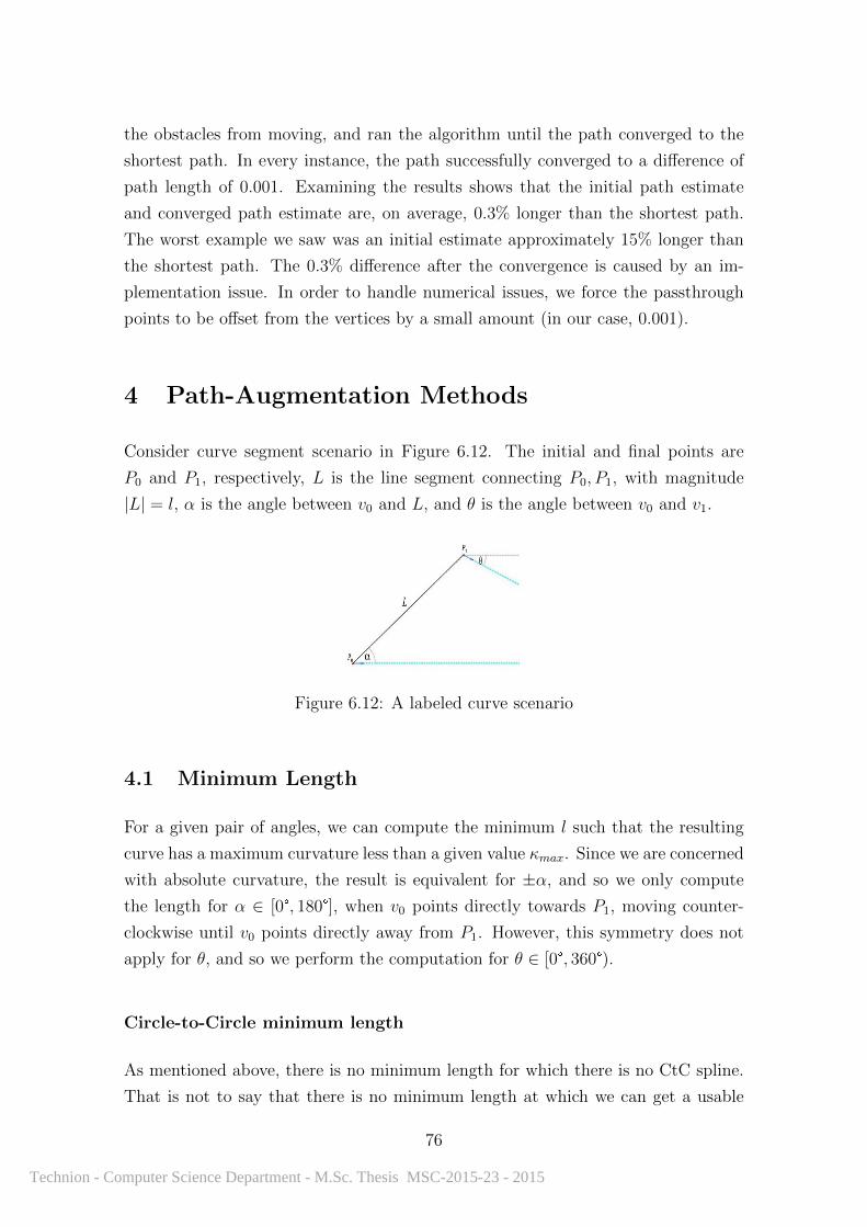
the obstacles from moving, and ran the algorithm until the path converged to the

shortest path. In every instance, the path successfully converged to a difference of

path length of 0.001. Examining the results shows that the initial path estimate

and converged path estimate are, on average, 0.3% longer than the shortest path.

The worst example we saw was an initial estimate approximately 15% longer than

the shortest path. The 0.3% difference after the convergence is caused by an im-

plementation issue. In order to handle numerical issues, we force the passthrough

points to be offset from the vertices by a small amount (in our case, 0.001).

4 Path-Augmentation Methods

Consider curve segment scenario in Figure 6.12. The initial and final points are

P0 and P1, respectively, L is the line segment connecting P0, P1, with magnitude

|L| = l, α is the angle between v0 and L, and θ is the angle between v0 and v1.

Figure 6.12: A labeled curve scenario

4.1 Minimum Length

For a given pair of angles, we can compute the minimum l such that the resulting

curve has a maximum curvature less than a given value κmax. Since we are concerned

with absolute curvature, the result is equivalent for ±α, and so we only compute

the length for α ∈ [0°, 180°], when v0 points directly towards P1, moving counter-

clockwise until v0 points directly away from P1. However, this symmetry does not

apply for θ, and so we perform the computation for θ ∈ [0°, 360°).

Circle-to-Circle minimum length

As mentioned above, there is no minimum length for which there is no CtC spline.

That is not to say that there is no minimum length at which we can get a usable

76


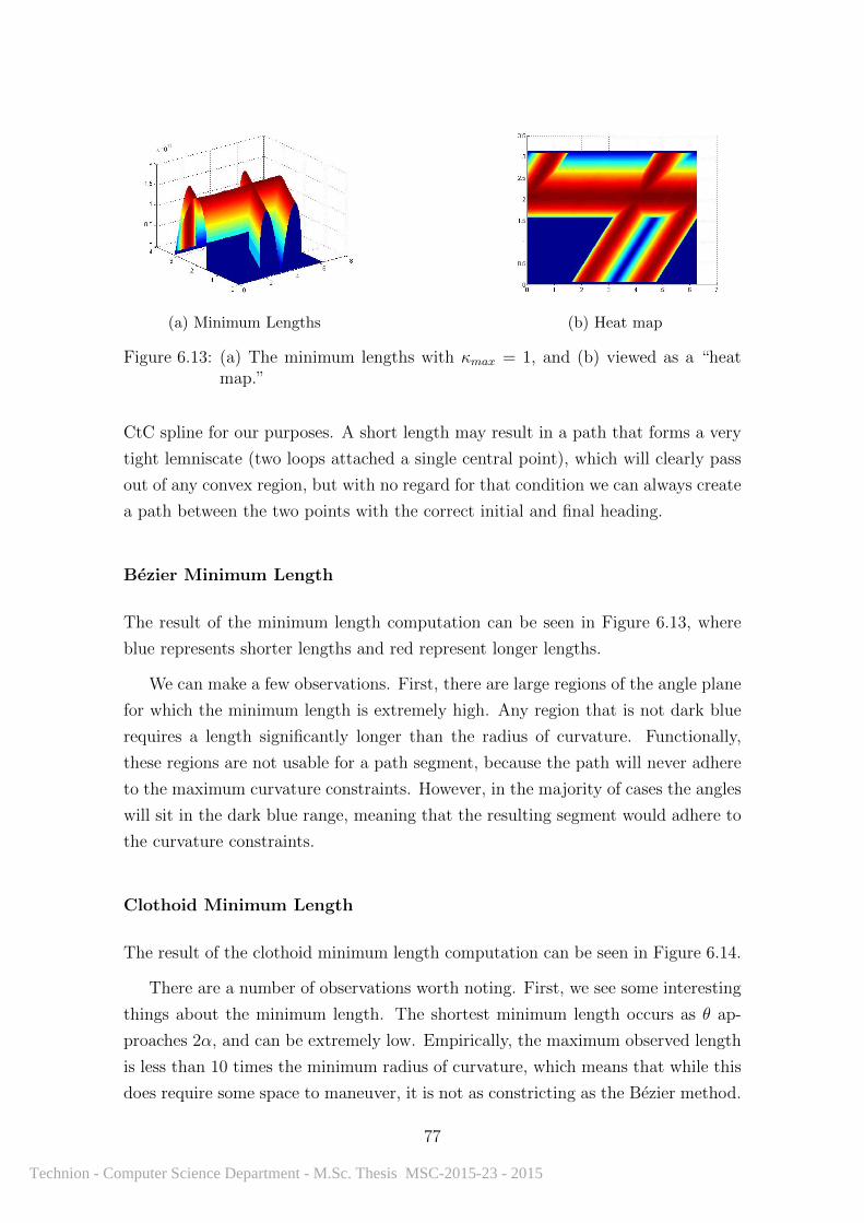
(a) Minimum Lengths (b) Heat map

Figure 6.13: (a) The minimum lengths with κmax = 1, and (b) viewed as a “heatmap.”

CtC spline for our purposes. A short length may result in a path that forms a very

tight lemniscate (two loops attached a single central point), which will clearly pass

out of any convex region, but with no regard for that condition we can always create

a path between the two points with the correct initial and final heading.

Bezier Minimum Length

The result of the minimum length computation can be seen in Figure 6.13, where

blue represents shorter lengths and red represent longer lengths.

We can make a few observations. First, there are large regions of the angle plane

for which the minimum length is extremely high. Any region that is not dark blue

requires a length significantly longer than the radius of curvature. Functionally,

these regions are not usable for a path segment, because the path will never adhere

to the maximum curvature constraints. However, in the majority of cases the angles

will sit in the dark blue range, meaning that the resulting segment would adhere to

the curvature constraints.

Clothoid Minimum Length

The result of the clothoid minimum length computation can be seen in Figure 6.14.

There are a number of observations worth noting. First, we see some interesting

things about the minimum length. The shortest minimum length occurs as θ ap-

proaches 2α, and can be extremely low. Empirically, the maximum observed length

is less than 10 times the minimum radius of curvature, which means that while this

does require some space to maneuver, it is not as constricting as the Bezier method.

77


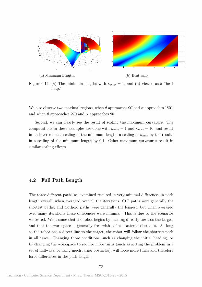
(a) Minimum Lengths (b) Heat map

Figure 6.14: (a) The minimum lengths with κmax = 1, and (b) viewed as a “heatmap.”

We also observe two maximal regions, when θ approaches 90°and α approaches 180°,

and when θ approaches 270°and α approaches 90°.

Second, we can clearly see the result of scaling the maximum curvature. The

computations in these examples are done with κmax = 1 and κmax = 10, and result

in an inverse linear scaling of the minimum length; a scaling of κmax by ten results

in a scaling of the minimum length by 0.1. Other maximum curvatures result in

similar scaling effects.

4.2 Full Path Length

The three different paths we examined resulted in very minimal differences in path

length overall, when averaged over all the iterations. CtC paths were generally the

shortest paths, and clothoid paths were generally the longest, but when averaged

over many iterations these differences were minimal. This is due to the scenarios

we tested. We assume that the robot begins by heading directly towards the target,

and that the workspace is generally free with a few scattered obstacles. As long

as the robot has a direct line to the target, the robot will follow the shortest path

in all cases. Changing those conditions, such as changing the initial heading, or

by changing the workspace to require more turns (such as setting the problem in a

set of hallways, or using much larger obstacles), will force more turns and therefore

force differences in the path length.

78


4.3 Algorithmic Failures

There are a number of possible pitfalls with the algorithm. The first such issue

is situations in which the complexity of the workspace gets extremely high. Our

algorithm requires a complete processing of the entire workspace every iteration.

We could potentially have a scenario in which there are an extremely large number

of obstacles, so much so that we cannot fully process the workspace in real time.

If any individual obstacle has a large number of vertices, we can approximate the

obstacle as a simpler polygon. If, however, there are a large number of obstacles, we

cannot simplify the model without artificially merging obstacles. This situation is

more problematic with curves such as the clothoid, due to the expensive computation

of the curve segments, but can be an issue with any curve type, if the number of

obstacles can get high enough.

A number of potential methods for handling these situations exist. We could

follow the approach of the local methods, and limit our search graph to a fixed

number of steps, or we could only augment the actual path, rather than the entire

graph. These methods are useful, but in the case of extremely large numbers of

obstacles, these actions may not be enough. A more extreme method is to bound

our work to a subspace of the workspace. This will violate many of our assumptions,

specifically that the workspace is static and that the obstacles remain fully bounded

within the workspace, but adaptations can be made to handle these cases.

A second potential issue with the algorithm is the case where the robot gets cor-

nered in a position such that the robot cannot move without violating the curvature

constraint. We try to prevent this by using the panic mode, and by disallowing travel

through gates that we deem too short, but even so we may still become trapped.

This would be because we moved towards a gap that suddenly closed. How these

cases will be handled must be determined by the user of the system. The user may

choose to allow violations of the curvature constraints, or may allow the robot to

reverse.

79



Chapter 7

Conclusions

We have developed a new framework for motion planning around mobile obstacles.

While previous methods are variants on the case of stationary obstacles, our new

method is specifically designed to operate in the dynamic case. We have shown that

the geometric framework upon which the path is built is correct, and stable. We

have also shown that each iteration can be done in linear time, with respect to the

complexity of the workspace, and each iteration results in a fully correct geometric

framework that is similar to the previous iteration but correct for the current layout.

The resulting linear-path graph can then be maintained and iteratively improved

and corrected in linear time as well. The linear path can then easily be augmented

to allow for a minimum radius of curvature, with a variety of path types based on

the users needs and constraints.

The path-augmentation methods each have strengths and weaknesses, and are by

no means the only possible augmentation methods. The CtC method results in the

shortest paths, and is the most stable for computation. However, the sudden changes

of curvature are difficult for people to handle, which is why roads, roller coasters,

and other paths are designed with a gradual change in curvature. Therefore, for

manned autonomous vehicles this is not a feasible method. Furthermore, no robotic

system can truly do the sudden changes of curvature, so it is an approximation at

best. The Clothoid curve is the smoothest, so best suited for people. However,

it results in the longest path, and is the heaviest to compute. The Bezier curve

is a good intermediate in terms of change in curvature and curve length, but in

many cases a result cannot be computed that adheres to our curvature constraints.

Therefore, each method would work best in specific circumstances, such as using

the Bezier curve in a scenario with small, fast-moving obstacles, or using the CtC in

81


unmanned vehicles, and using the Clothoid in cases when a smooth ride is prioritized.

Other methods will have their own pros and cons, and should be considered as well.

There are many avenues of future research. The framework we developed assumes

a point robot in the plane, a fixed workspace, and rigid obstacles that are always

bounded by the workspace. Future development could focus on removing any of

these assumptions. We could advance the framework to work with polygonal robots,

to work in three dimensions, or allow robots that are not rigid, or that can enter

and exit a workspace that can be static or changing.

82


Bibliography

[1] M. Abramowitz. Handbook of Mathematical Functions, With Formulas, Graphs,and Mathematical Tables,. Dover Publications, Inc. 1974.

[2] M. de Berg, O. Cheong, M. van Kreveld, and M. Overmars. ComputationalGeometry: Algorithms and Applications. Springer-Verlag TELOS, Santa Clara,CA, 3rd ed. edition, 2008.

[3] E. Bertolazzi and M. Frego. G1 fitting with clothoids. Mathematical Methodsin the Applied Sciences, 38(5):881–897, 2015.

[4] Radhakrishna Bettadapura, Tim Mashburn, and Richard Crawford. Length-constrained bezier curve smoothing. perpetually) in preparation, http://users.ices. utexas. edu/˜ brrk, 2012.

[5] P. Bezier. Numerical control; mathematics and applications [by] P. Bezier. Ap-pendixes by A. R. Forrest. Translated by A. R. Forrest and Anne F. Pankhurst.J. Wiley London, New York, 1972.

[6] D.M. Bond, N.A. Widgeon, W. Ruml, and X. Sun. Real-time search in dynamicworlds. In Proc. of the Third Ann. Symp. on Combinatorial Search, pages 16–22, Atlanta, GA, 2010.

[7] George Merrill Chaikin. An algorithm for high-speed curve generation. Com-puter graphics and image processing, 3(4):346–349, 1974.

[8] B. Chazelle. Triangulating a simple polygon in linear time. Discrete & Com-putational Geometry, 6(1):485–524, 1991.

[9] P.J. Davis. Interpolation and approximation. Dover Publications, New York,1975. Includes index.

[10] Gerald Farin. Curves and surfaces for computer-aided geometric design: apractical guide. Elsevier, 2014.

[11] Y.K. Hwang and N. Ahuja. Gross motion planning — a survey. ACM Comput.Surv., 24(3):219–291, September 1992.

[12] L.E. Kavraki, P. Svestka, J.-C. Latombe, and M.H. Overmars. Probabilisticroadmaps for path planning in high-dimensional configuration spaces. IEEETrans. on Robotics and Automation, 12(4):566–580, August 1996.

83


[13] S. Koenig and M. Likhachev. Real-time adaptive a*. In Proc. of the FifthInternational Joint Conference on Autonomous Agents and Multiagent Systems,AAMAS ’06, pages 281–288, New York, NY, 2006. ACM.

[14] S. Koenig and X. Sun. Comparing real-time and incremental heuristic searchfor real-time situated agents. Autonomous Agents and Multi-Agent Systems,18(3):313–341, 2009.

[15] R.E. Korf. Real-time heuristic search. Artificial Intelligence, 42(2-3):189–211,March 1990.

[16] J.-C. Latombe. Exact cell decomposition. In Robot Motion Planning, volume124 of The Springer International Series in Engineering and Computer Science,pages 200–247. Springer US, 1991.

[17] S.M. Lavalle. Rapidly-exploring random trees: A new tool for path planning.Technical report, Dept. of Computer Science, Iowa State University, 1998.

[18] M. Likhachev and D. Ferguson. Planning long dynamically feasible maneuversfor autonomous vehicles. Int. J. Robotics Research, 28(8):933–945, 2009.

[19] R.A. Liming. Practical Analytic Geometry with Applications to Aircraft. MacMillan, 1944.

[20] K. Macek and R. Siegwart. Motion planning in the presence of moving obstaclesusing ”rrt search” and ”b-splines”. In Robot Control, volume 8, pages 647–652.IFAC, 2006.

[21] R.R. Murphy. Introduction to AI Robotics. MIT Press, Cambridge, MA, 1stedition, 2000.

[22] J. O’Rourke. Art Gallery Theorems and Algorithms. International Series ofMonographs on Computer Science, No 3. Oxford University Press, 1987.

[23] Joseph O’Rourke. Computational Geometry in C. Cambridge University Press,second edition, 1998.

[24] F.P. Preparata and K.J. Supowit. Testing a simple polygon for monotonicity.Information Processing Letters, 12(4):161–164, 1981.

[25] E. Rimon and D.E. Koditschek. Exact robot navigation using artificial potentialfunctions. IEEE Trans. on Robotics and Automation, 8(5):501–518, October1992.

[26] I.J Schoenberg. On spline functions, with a supplement by t. n. e. greville,inequalities. In O Shisha, editor, Proc. of a Symp. held at Wright-PattersonAir Force Base, New York, 1967. Academic Press.

[27] N.H. Sleumer and N. Tschichold-Gurman. Exact cell decomposition of arrange-ments used for path planning in robotics, 1999.

84



v

או , שהמכשולים אינם קשיחים, אפשר להניח שהרובוט הוא מצולע. אפשרויות רבות להמשך המחקר ופיתוחויש

.ניתן לפתח סוגי מסלולים נוספים שיעבדו עם המערכת, כמו כן. להרחיב את המחקר לתלת מימד

Bibliography

Bertolazzi Enrico, and Frego Marco, G1 Fitting with Clothoids, Math. Meth. Appl. Sci., 38: 881–

897, doi:10.1002/mma.3114, (2015)


iv

ידוע שאורך . אבל ניתן לחשב אורך משוער. מקסימאלית שלואי אפשר לחשב בדיוק את אורך הקטע או העקמומיות ה

אנו מניחים שיש לכל היותר (. סדרת נקודות השליטה)חסום מלמעלה על ידי אורך מצולע השליטה שלה Bézierעקומת

אם יש לעקמומיות של הקטע, לכן. וניתן לאשש הנחה זו על ידי ניסוי, שתי נקודות מקסימום של עקמומיות בתוך הקטע

, על ידי הבנייה. יש לעקמומיות מקסימום גלובלי בתחילתו וסופו של הקטע, מקסימום מקומי בתחילתו וסופו של הקטע

.וגם בסופו של הקטע, העקמומיות בתחילת הקטע שווה לסף שקבענו

עם תכונה זו אומרת שקו לא יכול להיחתך. Variation Diminishing היא שהן Bézierתכונה נוספת של עקומות

אם כל ארבע נקודות שליטה , כלומר. העקומה מספר פעמים רב יותר מאשר מספר החיתוכים עם מצולע השליטה

אפשר . ולכן יש לבדוק רק אם נקודות השליטה האמצעיות בתוך הקטע, אז כל הקטע בתוך הפאה, נמצאות בתוך הפאה

.לבדוק זאת בקלות על ידי שימוש החסמים

הספירלה היא פונקציה פרמטרית המאופיינת על ידי עקמומיות המשתנה באופן . ת אוילרהעקומה שלישית היא ספירל

משוואת העקומה היא מן הצורה . לינארי

𝑥(𝑠) = 𝑥0 +∫ 𝑐𝑜𝑠𝑠

0

(1

2𝜅`𝜏2 + 𝜅𝜏 + 𝜃0)𝑑𝜏

𝑦(𝑠) = 𝑦0 +∫ 𝑠𝑖𝑛𝑠

0

(1

2𝜅`𝜏2 + 𝜅𝜏 + 𝜃0)𝑑𝜏

אשר מצאו דרך לחשב את קטע הספירלה הכי קצר המתחיל בנקודה Bertolazzi-ו Fregoעשינו שימוש בתוצאה של

, תוצאות החישוב הן אורך הקטע. וזו בדיוק הבעיה שלנו, ומסתיים בנקודה עם כיוון מסוים, מסוימת עם כיוון מסויים

. והשינוי בעקמומיות לאורך הקטע, העקמומיות ההתחלתית

אין שום דרך לזרז את . קסימלית היא בתחילת הקטע או בסופווהעקמומיות המ, אורך הקטע הוא תוצאה של החישוב

.בדיקת התיחום

ובמקרה הגרוע ביותר האלגוריתם , 𝑛-רוב האיטרציות מסיימות בזמן לינארי ב; מצאנו שהאלגוריתם שלנו עובד ביעילות

שון המתקבל לאחר המסלול הרא(. הוא מספר הצמתים של סביבת העבודה והמכשולים יחד 𝑛כאשר ) 𝑂(𝑛2)רץ בזמן

והתהליך מתכנס למסלול האופטימלי תוך מספר קטן של , איטרציה אחת הוא קירוב טוב למסלול הקצר ביותר

המסלול המבוסס של המעגלים ניתן לחישוב מהיר . ניתן לראות שלכל סוג מסלול יתרונות וחסרונות. איטרציות

הספירלה נותנת לנו . יק חלק ואינו ראוי לתחבורה אנושיתאבל המסלול אינו מספ, והמסלול הואקצר ביותר מכל השיטות

אבל החישוב כבד והמסלול הוא הארוך מבין , ואנו יודעים בדיוק את פרטי כל הקטעים, את המסלול החלק ביותר

Bézierעקומת . עלינו פשוט לבדוק את התשובה; חישוב הקטע אינו תלוי בסף על העקמומיות, כמובן. השיטות שנבדקו

המסלול ארוך יותר מהמסלול המתקבל . פשרות ביניים המחושבת בקלות והתיחום שלה נבדק בקלות באותה מידההיא א

הוא שאיננו יודעים בדיוק Bézierהחיסרון של עקומת . וקצר יותר מן המסלולים המבוססים על הספירלות, מן המעגלים

.את אורך המסלול ואת העקמומיות המקסימאלית של כל קטע


iii

ובעים את נקודות הכניסה אחר שק. ניתן לעדכן את המיקום הסופי וההתחלתי של הקטע וגם את הכיוון בו זמנית

עוברים על כל צאצאי הקטע ומעדכנים את הכיוונים הראשונים כדי , לאחר מכן. מחשבים רק את הכיוון הסופי, והיציאה

.שיהיו נכונים

לבדוק את ברצוננו למצוא שיטה, אם כך. והכיוונים ההתחלתי והסופי, בתהליך זה נתונות לנו נקודות ההתחלה והסוף

חוסם הכיוון ההתחלתי הוא הצלע של '.חוסם הכיוון הסופי'ו' חוסם הכיוון ההתחלתי'אנו מוצאים את . טעהתיחום של הק

ובאופן דומה עבור חוסם הכיוון , הפאה התוחמת אליה מגיעים כאשר יוצאים מהנקודה הראשונית בכיוון הראשוני

, וכאשר חל שינוי, רוב מאיטרציה לאיטרציההחסמים אינם משתנים על פי , מכיון שהמודל כולו זז באופן חלק. הסופי

.הוא מתבצע בדרך כלל לאחד מהשכנים

אנו יודעים שתחילתו של הקטע היא . עם החסמים אלו ביכולתנו לבדוק את התיחום של הקטע ביעילות עם התהליך הבא

ה ובודקים שלא אנו זזים קצת על העקומ. והוקטור הראשוני פונה לתוך הפאה, על אחת הצלעות של הפאה התוחמת

אם הוקטור בין הנקודות אינו . ובודקים שוב, זזים עוד קצת, עוברים לנקודה השנייה, אם כן. עברנו את החוסם הראשוני

כך . החסם הבא אמור להיות אחד מהשכנים של החוסם הנוכחי, מפני שהעקומה חלקה; מעדכנים את החסם, פונה לחסם

.עקומה או עד ליציאה מהפאהאנו ממשיכים עד אשר אנו מגיעים לסוף ה

עבורם אנו מסוגלים לחשב את המצבים הסופיים והעקמומיות , פיתחנו במערכת שלנו שלושה סוגים של עקומות

המשך התנועה , המאפיין שלה היא פניה בעקמומיות המקסימאלית.' מעגל למעגל'העקומה הראשונה היא . המקסימאלית

, מעגל נוסף המשיק לוקטור הסופי, בונים מעגל המשיק לוקטור הראשוני .ואז פניה שוב עד סוף התנועה, בקו ישר

מתקבלים יש . ומחפשים את המשיק אשר נותן המסלול הקצר ביותר, מחשבים את הקווים המשיקים לשני המעגלים

ם לכל זוג מעגלים יש רק משיק אחד שעובר בכיווני. ולכל זוג ארבעה משיקים משותפים, ארבעה זוגות של מעגלים

הכיוון נקבע על ידי המכפלה הפנימית בין הוקטור המשיק . כלומרבכיוונים של הוקטורים בנקודות הסיום, הנכונים

, יש ארבע אפשרויות(. ושלילי מסמן נגד כיוון השעון, חיובי מסמן בכיוון השעון)והנגזרת של המעגל בנקודת ההשקה

אנו בוחרים בזוג אשר נותן את המסלול . אורך הקו המשיקולכל אחת ניתן לחשב את אורך הקשתות של המעגלים ואת

.הקצר ביותר

אפשר . העקמומיות של המעגלים, על ידי בנייה, העקמומיות המקסימאלית היא. אורך הקטע הוא תוצאה של החישוב

.זמנית משני הכיוונים עד שמגיעים לקטע הישר-לשפר את בדיקת התיחום על ידי זחילה בו

הנקודה . העקומה בנויה מאינטרפולציה של ארבע נקודות שליטה. מדרגה שלוש Bézierהעקומה השנייה היא עקומת

אחד ממאפייני . והנקודה האחרונה היא הנקודה הסופית, הראשונה של העקומה היא הנקודה ההתחלתית של הקטע

, ור מנקודת השליטה הראשונה לשנייההוא שהכיוונים של תחילתה וסופה של העקומה שווים לוקט Bézier עקומת

והאורך בין הנקודה , יש לחשב את האורך מהנקודה הראשונה לשנייה, לכן. ובהתאמה לזה ומן השלישית לרביעית

.פיתחנו משוואה אשר קובעת את האורכים האלו. השלישית לרביעית כדי לחשב את כל העקומה


ii

אז עוברים על כל השערים ומבטלים את . פאות קמורות( או יותר)ואם הפאה קעורה מחלקים אותה לשתים , הפירוק

.השערים המיותרים

בעלת לכל קשת . כל קשת צריכה לזכור את האב ואת רשימת הצאצאים שלה. בצעד השני אנו בונים את גרף החיפוש

הצמתים של גרף , בדרך כלל. זה אשר יביא אותנו ליעד במסלול הקצר ביותר, בוחרים את הצאצא הטוב ביותר, צאצאים

על כל קשת לשמור את , לכן. הצמתים שלנו אינם נקודות אלא קטעי קווים. החיפוש הם נקודות בסביבת העבודה

.המיקום הראשון והאחרון שלה בשערים

מציבים את . מוסיפים את הקשתות עד שמתקרבים למסלול הקצר ביותר. מתחילים מהרובוט, ףכשמוסיפים קשתות לגר

ומציבים את נקודת היציאה לנקודה בשער היציאה שממזער את המרחק מנקודת , נקודת הכניסה ליציאתו של האב

, כל הצאצאיםלכל קשת אנו מטפלים ב. אנו משפרים את המסלול, כשהקשת כבר קיימת. הכניסה ליעד דרך השער

אין צורך לעשות , אם היציאה היא היעד. ורק אז עוברים לאב, מחשבים את נקודת הכניסה, מציבים את נקודת היציאה

אם יש לה . אז מחשבים את נקודת היציאה כמו שעשינו כאשר הוספנו את הקשת לגרף, אם אין לקשת צאצאים. דבר

אחר שקבענו את נקודת . יציאה על הכניסה של הצאצא הנבחרושמים את ה, בוחרים את הצאצא האופטימלי, צאצאים

קובעים את נקודת הכניסה להיות המקום בשער הכניסה שממזער את אורך המסלול מכניסתו של האב ליציאתה , היציאה

.של הקשת הנוכחית העוברת דרך השער

ספנו שער לפירוק שחתך קשתות אם הו. מתחילים מהרובוט ועוברים על הגרף לעומק: אנו מעדכנים את כל הגרף כך

מורידים את הצומת ושוב , אם הורדנו שער שיש לו צומת בגרף. ומעדכנים את הקשתות, מוסיפים צומת לגרף, בגרף

. ואז מעדכנים את נקודות הכניסה והיציאה של הקשת, מעדכנים את כל הצאצאים. מעדכנים את הקשתות

והכיוון , כל קשת בגרף הופכת לקטע של עקומה. עליון על העקמומיותבשלב השלישי אנחנו בונים מסלול חלק עם חסם

(. 1Gמה שנקרא רציפות )של הנגזרת בסוף הקטע צריך להיות שווה לכיוון של הנגזרת בתחילת הצאצא הכי טוב שלה

קטע כל , ראשית: לא תוכננה עבור סוג מיוחד של עקומה אלא עבור כל עקומה עם המאפיינים הבאים המערכת שלנו

אנו . כל קטע צריך לשבת באותו אזור של הפירוק שבו הקטע הליניארי עובר, שנית. צריך להיות גזיר לאורך כל הקטע

עלינו להיות , נוסף על כך .זקוקים ליכולת לחשב או להעריך את אורך הקטע ואת העקמומיות המקסימלית של הקטע

אנו זקוקים לאמצעים לבנות את העקומה רק מתנאי , לסיום. יכולים לוודא שכל הקטע יושב בתוך אותה פאה מהפירוק

(.המיקום והכיוון של תחילת וסוף הקטע)הקצה

. ועתה אנו מחשבים את הכיוונים של העקומה בשני קצותיה, יש לנו מבניית גרף החיפוש את מיקומן של נקודות הקצה

לחוצה של הקשתות ( סיבוב של תשעים מעלות)אנחנו קובעים את הכיוון הראשוני בניצב , כאשר אנו בונים את הקטע

כאשר . הכיוון הסופי שלו הוא החוצה של הקשת שלו והוקטור מהנקודה הסופית ליעד. הליניאריות שלו ושל אביו

.מעדכנים רק את שני הכיוונים, מעדכנים את הקשת


i

תקציר

בהינתן אזור .ו הראשוני עד יעדו הסופיהוא תהליך של בניית רצף של תנועות שיביא רובוט ממיקומ" תכנון תנועה"

בונים מסלול שיושב בתוך סביבת העבודה ואינו מתנגש באף , מכשולים ויעד", סביבת עבודה"המכונה , תחום במישור

זאת מכיוון שדבר לא משתנה . קיימים מגוון פתרונות לבעיית תכנון תנועה בנוכחות מכשולים נייחים .אחד מהמכשולים

כאשר , בניגוד לכך .(לכל הגדרת אופטימליות נדרשת)ולכן ניתן לחשב את המסלול האופטימלי , מתחילת התנועה

האלגוריתמים הקיימים הם וריאציות של האלגוריתמים . אין פיתרון אופטימלי שרץ בזמן אמת, המכשולים ניידים

הסטטיים איטיים מדי מכדי האלגוריתמים .הסטטיים המחשבים כל פעם מחדש את הפתרון בהתאם לשינויים במכשולים

אם , בנוסף לכך. נוכל לחשב את המסלול מחדש כך שבכל איטרציה לכן יש צורך לערוך בהם שינויים, לרוץ בזמן אמת

אין דרך , וברצוננו להחליק אותו עם חסם על עקמומיות מוחלטת מקסימלית(, למקוטעין)המסלול שבנינו הוא לינארי

תוך כדי , יתחנו אלגוריתם שיכול לחזור ולהשתמש באותו מידע מאיטרציה לאיטרציהבעבודה זו פ. יעילה לעשות זאת

ל.שלנו מאפשר החלקה יעילה של המסלוהאלגוריתם . עדכון המסלול בין האיטרציות

סביבת העבודה היא , המכשולים הם מצולעים וקשיחים, סביבת העבודה היא מצולע: הנחות העבודה שלנו הן כדלקמן

כל האלגוריתמים . בנוסף אנו מניחים שהרובוט נקודתי והוא זז באופן חלק. ולים זזים באופן חלקוהמכש, סטטית

כלומר את , האלגוריתמים בונים גרף חיפוש שמכסה את האזורים הפנויים. פחות או יותר באותו אופן הקיימים פועלים

ודה כצמתים בגרף החיפוש ומחפשים בוחרים נקודות בסביבת העב .אזורי סביבת העבודה שאינם מכוסים במכשולים

אנו מפרקים את האזורים הפנויים לפאות . אלא קטעי קווים, הצמתים בגרף שלנו אינם נקודות. מסלול בתוך הגרף

כלומר צלעות בין צמתים של סביבת העבודה או , למודל" שערים"אנו מוסיפים , כדי לאפשר את הפירוק. קמורות

עכשיו בונים . ושני שערים אינם יכולים להתנגש זה עם זה, כולו בתוך האזורים הפנוייםכל שער צריך לשבת . מכשולים

והקשתות המחברות בין , הצמתים של הגרף הם השערים שהוספנו. גרף חיפוש על הגרף הדואלי של הפירוק הקמור

וממשיך בכיוון , וטהגרף מכוון כך שכל מסלול מתחיל מהרוב. צמתים בגרף הן צלעות על הגבול של מצולע הפירוק

.והופכים את המסלול לסדרת עקומות חלקות, מחפשים מסלול בגרף, לבסוף. היעד

, האזור הפנוי שלנו הוא מצולע עם חורים, באתחול. הצעד הראשון של האלגוריתם הוא הפירוק הקמור של האזור הפנוי

למצולע על מנת לבטל ( אלכסונים)אנו מוסיפים שערים . כאשר סביבת העבודה היא המצולע והמכשולים הם החורים

עד לפירוק כל האזור , מכאן אנו מוסיפים שערים נוספים באופן חמדני. את החורים עד שמתקבל מצולע קעור בלי חורים

אם יש שער : ובודקים האם הם אכן נחוצים, בשלב זה אנו חוזרים אל כל השערים שהוספנו. הפנוי לפאות קמורות

אנו מסירים אותו כדי לאחד את שני המצולעים למצולע אחד גדול יותר אך , שני צמתים קמורים של מצולעשמחלק

.עדיין קמור

ואין שנויים רבים במצבו , שהכשולים זזים במידה מועטת בין שתי איטרציות,אנו מניחים שהתזוזה של המכשולים חלקה

בודקים את כל הפאות של. שתמש בפירוק ורק לתקן אותוהנחת היסוד שלנו היא שניתן לה, לכן. של הפירוק שלנו



גיל ברקת בפקולטה למדעי המחשב' ה בהנחיית פרופהמחקר נעש



תכנון תנועה בנוכחות מכשולים ניידים

חיבור על מחקר לשם מילוי חלקי של הדרישות לקבלת התואר מגיסטר למדעים במדעי המחשב

סטיפל( אברהם)אבי

מכון טכנולוגי לישראל -הוגש לסנט הטכניון

2015יולי , חיפה, ה"אב תשע



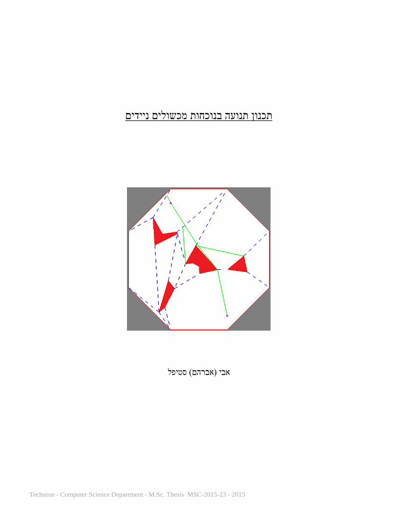
תכנון תנועה בנוכחות מכשולים ניידים

אבי )אברהם( סטיפל


Documents

Motion Planning in the Presence of Mobile Obstacles