Centre forEconomicand FinancialResearchatNew Economic School

Mortality in Russia:Microanalysis

Irina Denisova

Working Paper �o 128

CEFIR / �ES Working Paper series

March 2009

Mortality in Russia: Microanalysis

Irina DENISOVA Center for Economic and Financial Research and New Economic School,

Suit 720, Nakhimovsky 47, 117418, Moscow, Russia e-mail: idenisova@cefir.ru

Abstract The paper studies determinants of Russian adult mortality controlling for individual and household heterogeneity. We utilize twelve rounds of the Russian Longitudinal Monitoring Survey spanning the period of 14 years to study determinants of adult mortality. Survival analysis is the main methodology employed. The results are original in several respects. We find empirical support to the importance of relative status measured in non-income terms in shaping mortality hazards while income-measured relative position is confirmed to be statistically insignificant. We find evidence on the influence of labor market behavior, and sectoral and occupational mobility in particular, on longevity. The health detrimental role of smoking is found to be comparable to the role of excess alcohol consumption which is novel in the Russian context where the influence of smoking is downplayed in comparison to the alcoholism. Finally, we find no micro evidence in support to the regional data result underlying Treisman (2008) political economy story. Keywords: Mortality, Relative Deprivation, Survival Analysis, Transition, Russia JEL Classification: J1, J10, J18, I1, I12, D31

2

1. Introduction Dramatic changes in economic, social and cultural life of countries of Central and

Eastern Europe (CEE) and Former Soviet Union (FSU) induced by the reforms of the end of the

80-ies and the 90-ies could not have left untouched the well-being of families and individuals.

One of the potential dimensions of the influence is the effect on health, morbidity and mortality.

Indeed, many countries of the group demonstrated sizable increases in mortality and declines in

life expectancy at the initial years of the reform. For instance, male life expectancy decreased

cumulatively by 1.57 years in 1989-1994 in Hungary and by 0.97 years in 1989-1991 in Poland

(European health for all database, 2008). The decline in life expectancy in the Czech Republic,

however, was almost negligible and was quickly followed by a steady growth. At the same time,

the FSU countries experienced much more pronounced, especially for males, increases in

mortality rates and declines in life expectancy, with Russia being the leader. Moreover, many of

the countries of the FSU are still not back to the upward trend in life expectancy and experienced

another episode of sizeable decline after 1998. Male life expectancy from birth decreased

cumulatively by 5.82 years in 1992-94 and again by 2.71 years in 1999-2003 in Russia (Figure

A1 in Appendix). Female life expectancy in Russia experienced a decline by 2.6 years in 1992-

94 and by 1.38 years in 1999-2003. As a result, male life expectancy in Russia is one of the

lowest in Europe, and working age male mortality rate is among the highest.

The underlying factors behind the rise in mortality, and the role of the dramatic economic

transformations in particular, are still in the center of public and academic discussions (c.f.

Ellman, 1994, Andreev et.al., 1994, Chen et. al., 1996, Cutler, Deaton and Lleras-Muney, 2006).

Several explanations of the mortality crisis are considered: malnutrition and unhealthy diet due

to income decline and rise in poverty (Zohoori et.al., 1998); alcohol consumption/binge drinking

(Leon et.al., 1997, Shkolnikov et.al., 1998, Brainerd and Cutler, 2005), with a special role of

policy of low prices on vodka (Treisman, 2008); adverse expectations and exposure to stress

caused by shock therapy policies (Leon and Shkolnikov, 1999, Brainerd and Cutler, 2005),

including privatization (Stuckler et.al., 2009); deterioration of health care provision (Brainerd

and Cutler, 2005); deterioration of social capital (Kennedy et.al., 1998). The majority of the

papers focus on Russia as the sharpest case, with some interesting examples of studies on other

countries (Eberstadt, 1990, 1994 on Eastern Europe, Riphahn and Zimmermann, 1998 on Eastern

Germany; Brainerd and Cutler, 2005 on FSU countries).

A common approach is to utilize aggregate death certificate data to identify national and

regional all-causes and cause-specific death rates. The aggregate mortality data is then used to

test for the determinants of mortality patterns either on cross-section of countries (Brainerd and

3

Cutler, 2005, Stuckler et.al., 2009), or on a sample of regions in a country (Walberg et.al., 1998,

Treisman, 2008). The use of individual data is very limited with the examples in Brainerd and

Cutler (2005) on Russia and in Riphahn and Zimmermann (1998) on Eastern Germany. While

producing important insights into mortality determinants, aggregate data do not allow controlling

for household and individual heterogeneity thus limiting the strength of the tests. The paper is to

contribute to the discussion by testing for the importance of various factors on mortality in

Russia in 1994-2007 when controlling on the observable individual and household heterogeneity.

The study is based on the Russian Longitudinal Monitoring survey (RLMS) - a nationally

representative survey of more than 4,000 households run from 1992 with very rich individual

questionnaire and careful monitoring of household circumstances.

There are several novel results of the study. First, we find empirical support to the

longevity reducing role of relative deprivation and inequality measured on a non-income scale of

a self-perceived position on the respect ladder. A potential role of inequality in non-income

terms in shaping mortality and the lack of direct tests of this role is stressed in Deaton (2003). A

room for this factor is even higher in transition countries with the drastic changes in relative

status of large groups of people. Our study is the first direct test of this kind. We find that a

lower self-assessed status measured as respect from others increases mortality hazard.

In line with the individual level literature (c.f. Deaton, 2003), we find no influence of

relative position measured along monetary income scale on the risk of mortality when

controlling for the absolute income position. In addition, poverty spells are likely to be

hazardous to individual health, with the first poverty spell having the strongest influence which

is in line to the findings by Oh (2001) and Zick and Smith (2001) for the US.

Second, career-related factors, and the degree of flexibility in the labor market measured

as the observed frequent transitions between wage for wages and self-employment and

entrepreneurship, or downward occupational mobility, reveals being an important factor of

moderation of mortality risk. This adds micro-level evidence to the finding of Walberg et.al.

(1998) who report that high rates of labor turnover in regions are associated with higher

mortality rates: those who manage to adjust to the fast changes by accepting jobs in a different

sector and/or of a different qualification level have better chances to survive. An open question

here is what are the intrinsic characteristics of people that facilitate their adjustment in the labor

market?

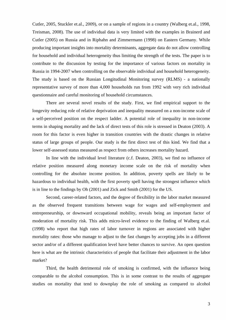
Third, the health detrimental role of smoking is confirmed, with the influence being

comparable to the alcohol consumption. This is in some contrast to the results of aggregate

studies on mortality that tend to downplay the role of smoking as compared to alcohol

4

consumption though the increase in tobacco consumption in transition is well documented (e.g.,

Perlman et.al., 2007).

Finally, the role of price of alcohol (vodka) in relative and absolute terms shows

insignificant in mortality determination, with a tendency, if any, for higher mortality when prices

are high. The likely mechanism behind the (weak) positive correlation is a hazardous substitution

towards cheaper and more toxic liquids documented by Andrienko and Nemtsov (2005). This is

in contrast to the regional-level result in Treisman (2008) who finds negative association

between regional crude death rates and regional vodka prices for 1993-2005 and interprets this as

a cost of the political populism and fearing of political opposition which put limits to vodka

prices and caused the increased consumption of hard liquors.

The paper is organized as follows. Section 2 describes the data and construction of

variables. Section 3 discusses the methodology applied. Section 4 discusses the results of the

study and considers robustness checks. Section 5 concludes.

2. Data and construction of variables The empirical basis of the study is the Russian Longitudinal Monitoring survey

(http://www.cpc.unc.edu/rlms), rounds 5-16 covering the period from 1994 to 2007. The data are

nationally representative and are based on the survey of more than 4,000 households per year

which amounts to more than 10,000 adults per year. The sample is a two-stage random draw of

dwellings from the population of the micro census of 1989. The dwellings are surveyed each

year, with some additional dwellings added in the later periods of the survey to meet the national

representation criteria. The dwelling-based longitudinal nature of the survey has some

advantages and some drawbacks as compared to the true panel with respect to our task. On the

one hand, the data are nationally representative in each year thus promising mortality rates closer

to the population rates when adjusted for the size of the sample. On the other hand, there is a

potential attrition bias due to the fact that some households leave the sample as they move out of

the dwelling. The attrition issue is discussed in more detail below.

2.1 Dependent variable

The death event is registered in the sample on the basis of the information provided by

the household head when the unit is surveyed at least two rounds in a row. A household head is

asked to report whether any household member is missing during this survey round and the

reason for that member being not in the household. One of the reasons reported is the death of

the household member. Starting from 2001 the cause of the death is also reported. Along the

period of thirteen years 1,245 adult persons (5% of the adults in the sample throughout the

5

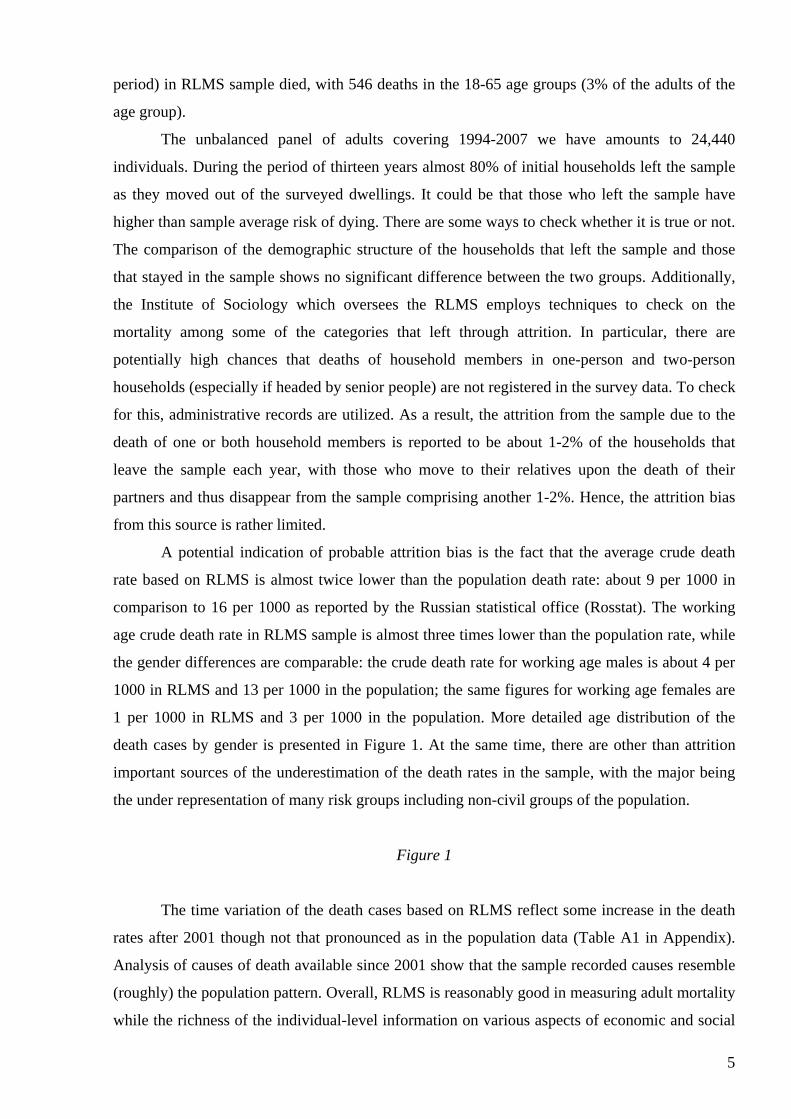
period) in RLMS sample died, with 546 deaths in the 18-65 age groups (3% of the adults of the

age group).

The unbalanced panel of adults covering 1994-2007 we have amounts to 24,440

individuals. During the period of thirteen years almost 80% of initial households left the sample

as they moved out of the surveyed dwellings. It could be that those who left the sample have

higher than sample average risk of dying. There are some ways to check whether it is true or not.

The comparison of the demographic structure of the households that left the sample and those

that stayed in the sample shows no significant difference between the two groups. Additionally,

the Institute of Sociology which oversees the RLMS employs techniques to check on the

mortality among some of the categories that left through attrition. In particular, there are

potentially high chances that deaths of household members in one-person and two-person

households (especially if headed by senior people) are not registered in the survey data. To check

for this, administrative records are utilized. As a result, the attrition from the sample due to the

death of one or both household members is reported to be about 1-2% of the households that

leave the sample each year, with those who move to their relatives upon the death of their

partners and thus disappear from the sample comprising another 1-2%. Hence, the attrition bias

from this source is rather limited.

A potential indication of probable attrition bias is the fact that the average crude death

rate based on RLMS is almost twice lower than the population death rate: about 9 per 1000 in

comparison to 16 per 1000 as reported by the Russian statistical office (Rosstat). The working

age crude death rate in RLMS sample is almost three times lower than the population rate, while

the gender differences are comparable: the crude death rate for working age males is about 4 per

1000 in RLMS and 13 per 1000 in the population; the same figures for working age females are

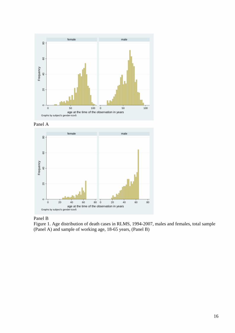
1 per 1000 in RLMS and 3 per 1000 in the population. More detailed age distribution of the

death cases by gender is presented in Figure 1. At the same time, there are other than attrition

important sources of the underestimation of the death rates in the sample, with the major being

the under representation of many risk groups including non-civil groups of the population.

Figure 1

The time variation of the death cases based on RLMS reflect some increase in the death

rates after 2001 though not that pronounced as in the population data (Table A1 in Appendix).

Analysis of causes of death available since 2001 show that the sample recorded causes resemble

(roughly) the population pattern. Overall, RLMS is reasonably good in measuring adult mortality

while the richness of the individual-level information on various aspects of economic and social

6

life together with the carefully measured household data makes it very attractive to study

determinants of mortality.

2.1 Explanatory variables

Scholars from different fields confirm that psycho-social stress is one of the important

factors behind deterioration of health and rise in mortality (e.g., Brunner, 1997, Riphahn and

Zimmermann, 1998). As defined in ‘economic terms’ by Shapiro (1995) stress is a condition in

which the individual perceives a discrepancy between the demands of the environment and the

available resources. The data allows measuring the exposure of individuals to stress along

several dimensions.

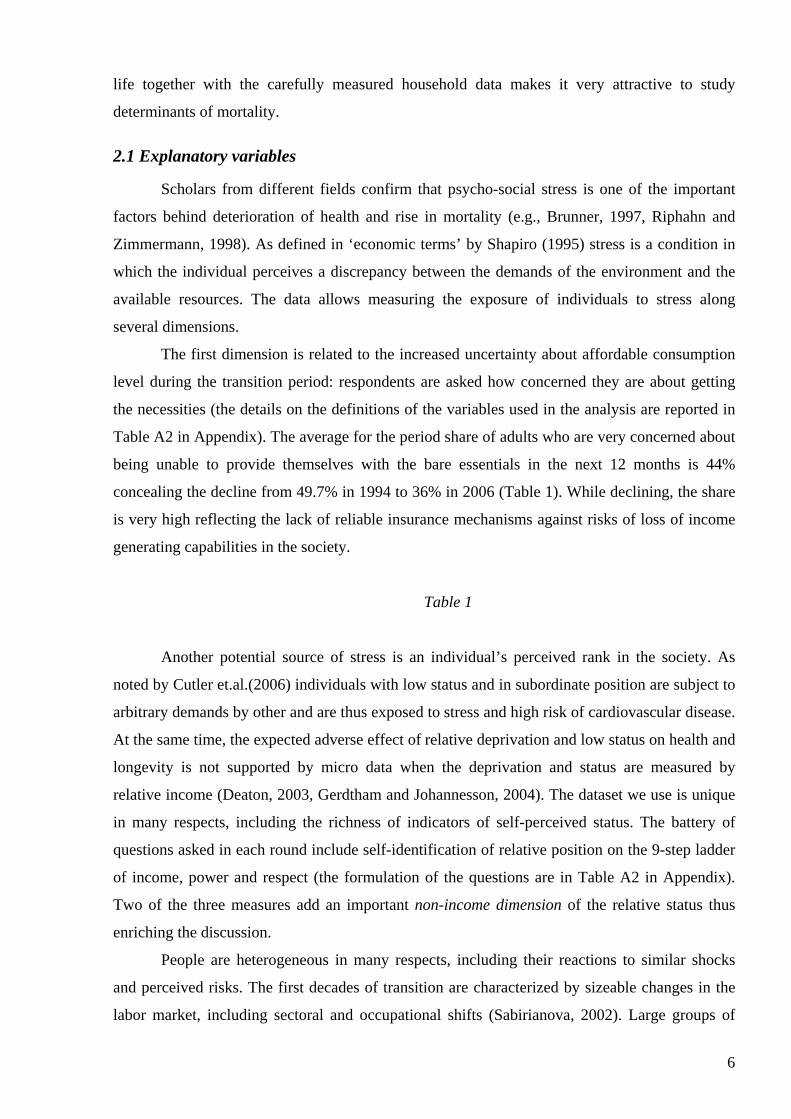
The first dimension is related to the increased uncertainty about affordable consumption

level during the transition period: respondents are asked how concerned they are about getting

the necessities (the details on the definitions of the variables used in the analysis are reported in

Table A2 in Appendix). The average for the period share of adults who are very concerned about

being unable to provide themselves with the bare essentials in the next 12 months is 44%

concealing the decline from 49.7% in 1994 to 36% in 2006 (Table 1). While declining, the share

is very high reflecting the lack of reliable insurance mechanisms against risks of loss of income

generating capabilities in the society.

Table 1

Another potential source of stress is an individual’s perceived rank in the society. As

noted by Cutler et.al.(2006) individuals with low status and in subordinate position are subject to

arbitrary demands by other and are thus exposed to stress and high risk of cardiovascular disease.

At the same time, the expected adverse effect of relative deprivation and low status on health and

longevity is not supported by micro data when the deprivation and status are measured by

relative income (Deaton, 2003, Gerdtham and Johannesson, 2004). The dataset we use is unique

in many respects, including the richness of indicators of self-perceived status. The battery of

questions asked in each round include self-identification of relative position on the 9-step ladder

of income, power and respect (the formulation of the questions are in Table A2 in Appendix).

Two of the three measures add an important non-income dimension of the relative status thus

enriching the discussion.

People are heterogeneous in many respects, including their reactions to similar shocks

and perceived risks. The first decades of transition are characterized by sizeable changes in the

labor market, including sectoral and occupational shifts (Sabirianova, 2002). Large groups of

7

people got exposed to the reallocation shocks. Some moved, and, say, left an engineering

position for a position of a salesman in a furniture store; others opted to stay at the low-paid

engineering position to avoid the downward shift along an occupational ladder. Which strategy is

more health detrimental? The empirical evidence is very scarce (e.g., Lazareva, 2008). The

detailed record of labor market history of individuals in our sample allows testing whether those

rather mobile in terms of changing sectors of employment and occupations benefit in terms of

higher longevity. We define those who experienced downward occupational mobility when

employed for wages or several movements between work for wages and self-employment or

entrepreneurship as being ‘mobile in the labor market’. There are 5% of mobile adults in our

total sample which amounts to 12% in the sample of working-age adults below 60 (Table 1).

There are social mechanisms to mitigate exposure to stress, formal and informal. When

formal institutes of social cohesion are underdeveloped, as in Russia, people rely on informal

sources of support, friends and family, to deal with their day to day problems (Kennedy et.al.

1998, Walberg et.al., 1998). Those lacking such sources of support are especially vulnerable to

economic hardships following transformation. There are several indicators of this dimension of

social capital available in the dataset: family related indicators (the size of the family, the

presence of children in family) and the settlement type (urban versus rural). The indicators are

rather broad and reflect other than social capital motives as well. The presence of children is

likely to discourage risk-taking behavior of parents (Umberson, 1987, Kotler and Winghard,

1989) thus adding to the social function. Larger families may induce higher concern about

getting necessities. Rural areas are likely to differ from urban areas in many respects, including

the life style and drinking and smoking patterns. Still, the social capital dimension of the

indicators is relevant as well. The mean demographic characteristics of the sample reported in

Table 1 confirm that the demographic structure of the sample is close to the one reported by

Rosstat on the Russian population.

Alcohol consumption considered by some persons as a stress-relieving strategy is viewed

as one of the key factors behind the abnormal (for the level of economic development) mortality

rates of the working age male population in Russia. The role of the factor is confirmed by the

analysis of cause-specific death rates during the period and is hardly challenged by anybody

(e.g., Leon et.al., 1997, Shkolnikov et.al., 1998, Gavrilova et.al., 2000). We test for the role of

the factor by distinguishing between binge drinkers defined as those who drink alcohol every day

or 4-6 times a week and the rest of the population. An alternative measure of binge drinking

based on the amount of alcohol consumed per day is believed to be a weaker measure since

respondents tend to misreport the alcohol intake (Andienko and Nemtsov, 2006). Additionally,

the question on the amount of alcohol intake changed in 2006 thus limiting its comparability

8

across periods. There are 3% of binge drinkers in our total sample, with 5.5% among working

age males and 1% among working age females.

We also test for the adverse effect of low alcohol prices documented in aggregate

regional-level data (Treisman, 2008) by controlling for the relative (to bread) and absolute price

of vodka (deflated to 1994 level) in a locality1. The variation in relative prices across localities is

sizeable: the mean across localities (lowest) price of one liter of vodka is about 7 times the price

of one kilogram of wheat bread, with the standard deviation of 3.6.

In addition to the role of the abuse of alcohol consumption we test for the influence of

smoking on longevity by controlling for the smoking habit. The well documented health

detrimental effect of smoking in general is somewhat downplayed in the Russian context despite

the unfavorable change in the pattern of smoking recorded with the increased youth and female

smoking rates (e.g., Arzhenovsky, 2006, Perlman et.al., 2007). More than 30% of adults in the

sample smoke, with the rate amounting to 60% for males. Note that we always control for the

education level (measured by the highest education degree achieved) as an important factor of

individual behavior including the choice of healthier lifestyles (Shkolnikov et.al., 1998).

The next group of variables is to capture the economic well-being of households

individuals live in. Absolute income is a well documented determinant of health and longevity,

and is proxied by household consumption. In addition to income, poverty has a potential of

increasing mortality risk via less healthy diet, limiting access to private medical care and to other

important consumption items (Duleep, 1986, Moore and Hayward, 1990, Zick and Smith, 1991).

The limitations are likely to expose family members to stress. Experience of long-term poverty

may be even more health detrimental though Oh (2001) shows that the first poverty spell is

especially potent in explaining the mortality risk, with the rest spells being less influential. We

allow the first and the next poverty spells induce differentiated influence on mortality risk.

Finally, we test for the influence of the deterioration in access to the qualified medical

care on the longevity by focusing on the medicine availability and affordability. Medicine

expenses are by and large privately financed in Russia with subsidization of the most vulnerable

groups. On average, five per cent of adults report having no money or failing to find the

prescribed medicine, with the share being higher at the initial years of transition and in 1998.

We control for individual health stock by both self-assessed health indicator and selected

objective measures of health including the body mass index and its square and the incidence of

heart attack, stroke and diabetes.

1 A locality is defined at the level of a community (site variable) in RLMS. There are about 150 communities in RLMS. The information on the infrastructure of the population center and the prices of basic food products is collected by interviewers in each locality each year. The community questionnaire is available at http://www.cpc.unc.edu/rlms.

9

3. Empirical Methodology The core methodology of our study is survival (duration) analysis. The approach allows

exploiting the features of longitudinal data and permits overcoming the estimation bias coming

from the problem of non-normality of the distribution for time to an event and of right-censoring

(c.f. Kiefer, 1988 for a survey). The approach is widely used for studies of mortality based on

micro data2. The central idea of the approach is to estimate the hazard rate defined as the

probability that the spell ends at time t conditional that the spell lasts till period t for the

observations with completed spells and to estimate survival function for the observations with

uncompleted or right-censored spells. In mortality studies the hazard rate at age t is the

conditional probability of dying at age t having survived to that age, and the survival rate at age t

is the probability of surviving till age t.

We use proportional hazard specification in which the hazard function is a product of a

baseline hazard and a term that shifts the baseline hazard proportionally in accord with the

influence of various covariates. The baseline hazard is a function of age.

( ) ( ) ( )txxt 00 ,,,, λβφλβλ = ,

where 0λ - base hazard function, corresponding to ( ) 1=⋅φ , ( ) ( )ββφ 'exp, xx = , x -

vector of explanatory variables, β - estimated coefficients. Two types of the baseline function

specifications are used. The first one is a parametric specification which assumes that the

baseline hazard is from the Gompertz class of distributions with an estimated gamma parameter.

The second specification is a flexible Cox proportional hazard model in which the base hazard

function is left unspecified. Robust Huber-White estimator of variance is applied to calculate

standard errors.

Given the modest number of death cases, we do not subdivide the sample into the sub-

samples of males and females but rather control for gender in the vector of explanatory variables

and allow for the gender specific baseline function in some specifications, both parametric and

non-parametric. In each case we also control for individual health stock by both self-assessed

health indicator and selected objective measures of health including the body mass index and its

square and the incidence of heart attack, stroke and diabetes.

The vector of explanatory variables x includes several groups of factors reflecting

competing theories discussed above: self-perceived social status; labor market related indicators

of stress and flexibility; health care accessibility; health detrimental habits and alcohol

2 For instance, Smith and Zick (1994) study mortality of husbands and wives using the Panel Study of Income Dynamics. Gerdtham and Johannesson (2004) use Cox model to test for the role of absolute and relative income in mortality using Swedish micro data.

10

availability; household economic well-being; individual human capital and social capital

indicators.

Kaplan-Meier estimates of survival functions being a convenient way of presenting the

dependent variable of our study provide support to both the choice of the Gompertz-class of the

parametric functions as the baseline hazard/survival (compare the two survival functions,

empirical and analytical, in the upper panel of Figure 2) and the choice of the explanatory

variables (the other panels in Figure 2).

Figure 2

4. Results The results of the estimates of proportional mortality hazard models on the sample of

working age (18-65) adults are reported in Table 2. Specifications 1 to 4 assume parametric

baseline hazards, with 3 and 4 letting the differentiation of the baseline hazard by gender.

Specifications 5 to 8 are Cox proportional hazard models, with 7 and 8 allowing for the baseline

hazard stratification on gender. Another difference between the specifications is the inclusion of

relative or absolute price of alcohol. Hazard ratios rather than coefficients are reported with

robust standard errors in brackets.

Let us start with the stress-related factors. The first group of the results highlights the role

of absolute and relative (income and non-income) position of a person in mortality. Controlling

for other factors, higher household income increases longevity, while poverty experience

decreases longevity. The first poverty spell is the most detrimental and increases mortality

hazard by almost 50 percentage points, with the next poverty episodes being statistically

insignificant.

Self-accessed relative position when measured along an income scale is statistically

insignificant with a tendency of a higher rank to lower mortality hazard rates. In contrast, respect

rank is significant in shaping mortality hazards. Those with higher self-assessed status measured

along the respect scale have lower mortality hazard: movement to a higher ladder step decreases

mortality hazard by 5.3 percentage points. Hence, we confirm the insignificance of income

measured relative deprivation and find empirical support to the role of non-income measured

relative deprivation.

An alternative measure of stress measured as the perceived high risk of being unable to

provide the bare essentials shows insignificant with a tendency to increase the mortality hazard.

11

Those who experienced frequent changes in the labor market including downward

occupational shifts show almost 50 percentage point lower mortality hazard rates. We interpret

this in favor of higher psychological flexibility of this group of respondents: those who moved

are likely to be more flexible not only in labor market terms but possibly in psychological terms

as well thus revealing better adjustment ability.

Health detrimental lifestyles, smoking and alcohol consumption do increase mortality

hazard rates. Importantly, smoking raises the mortality hazard as strong as binge drinking. Those

who smoke have 64 percentage points higher mortality hazard as compared to those who do not

smoke, and binge drinkers have 56 percentage point higher hazard rates. The result points to the

importance of anti-smoking measures as an integral part of health promoting policy.

Neither absolute nor relative price of alcohol (vodka) affect the hazard rates in our data.

If anything, we find a weak positive association between alcohol prices and mortality hazard

which could be attributed to the adverse effect of substitution for cheaper and toxic liquids.

The evidence with respect to the social capital measures we use is mixed. The presence

of children in family increases longevity by reducing hazard rate by 20 percentage points. At the

same time, living in an extended (larger) family increases mortality hazard by 15 percentage

points. The latter could reflect higher concern for getting necessities in larger families. Marital

status shows to be insignificant.

We find that living in urban area decreases mortality hazard by 23 percentage points. The

sign of the effect is in line with the aggregate data. We also confirm that better education is

beneficial for longevity: holders of university degree have almost 40 percentage point lower

mortality hazard rate.

Finally, a poor access to healthcare measured as inability to afford or find the prescribed

medicine show insignificant in shaping mortality hazard with a tendency to increase it.

Table 2

Table 3 presents results of the estimates of proportional mortality hazard models on total

sample of adults. The major results are the same with the most important difference being the

detrimental role of not only the first but also the next poverty spells. We should also notice the

unusual positive association of marriage and mortality hazard in our sample. The result is likely

to reflect the abnormally high gap between male and female life expectancy in Russia: majority

of pension-age females are widows in Russia which is in contrast to the developed countries.

Table 3

12

The results show to be robust across different specifications. The signs and the

significance levels are robust with respect to the parametric versus nonparametric baseline

hazard specification and survive allowing for gender stratification. It is only in some cases that

the magnitude of the coefficients changes slightly. Additional robustness checks came from

inclusion of the variables of interest by portions and by omission of the variables that could

potentially bias the results. For instance, we dropped the settlement type dummy and the binge

drinker variable when testing for the robustness of the price of alcohol result. The results did not

change.

5. Conclusions

Mortality crisis in countries of the Former Soviet Union and Russia in particular attracts

attention of academic and policy community. The majority of the studies are based on aggregate

data limiting the scope of the discussion to the measures available at national and sub national

level. The paper is one of the first to study determinants of Russian adult mortality controlling

for individual and household heterogeneity. The results are original in several respects.

First, we find empirical support to the importance of relative status measured in non-

income terms in shaping mortality hazards. Income-measured relative position is confirmed to be

statistically insignificant which is in line with the micro evidence from other countries.

Second, we find evidence on the influence of labor market behavior, and sectoral and

occupational mobility in particular, on longevity. We attribute the effect to the association of

higher mobility in the labor market and higher psychological flexibility. The effect could be

particularly noticeable during periods of sizeable structural changes like transition from plan to

market or adjustment to deep global crisis.

Third, the health detrimental role of smoking is found to be comparable to the role of

excess alcohol consumption. The result is novel in the Russian context where the influence of

smoking is downplayed in comparison to the alcoholism.

Finally, we find no micro evidence in support to the regional data result underlying

Treisman (2008) political economy story. If anything, there is a (very weak) positive association

between prices of hard alcohol and mortality hazard.

Statistical significance of the effects operating via relative non-income status and labor

market transitions which survives control for more traditional hazards of unhealthy lifestyles is a

confirmation of the adverse effects of economic transformations on adult longevity.

Mechanisms, formal and informal, to facilitate individual adjustment to the changed economic

and social environment are to be a part of mortality reducing policies.

13

References Andreev, E.M., V.A.Biryukov, and K.J.Shaburov (1994). “Life Expectancy in the Former USSR and Mortality Dynamics by Cause of Death: Regional Aspects”, European Journal of Population 10, pp.275-285. Andrienko and Nemtsov (2005). “Estimation of Individual Alcohol Demand,” Economics Education and. Research Consortium, Working Paper series, 05/10. Arzhenovsky, Sergei (2006). “Socioeconomic Determinants of Smoking in Russia,” Quantile Journal, Vol. 1, pp. 81-100. Baltagi, Badi H. and Ingo Geishecker (2006). “Rational Alcohol Addiction: Evidence from the Russia Longitudinal Monitoring Survey”, Health Economics, 15, pp.893-914. Braninerd, Elizabeth and David M.Cutler (2005). “Autopsy of an Empire: Understanding Mortality in Russia and the Former Soviet Union”, Journal of Economic Perspectives, 19, 1, pp.107-130. Brunner, Eric (1997). “Socioeconomic Determinants of Health: Stress and the Biology of Inequality,” British Medical Journal, 314:1472 Chen, Lincoln C., Friederike Wittgenstein, and Elizabeth McKeon. (1996). “The Upsurge of Mortality in Russia: Causes and Policy Implications”, Population and Development Review 22(3), pp.517-530. Deaton, Angus (2003). “Health, Inequality, and Economic Development,” Journal of Economic Literature, 41, 1, pp.113-58. Duleep, H.O.(1986). “Measuring the Effect of Income on Adult Mortality Using Longitudinal Administrative Records Data,” Journal of Human Resources, 21, pp.238-52. Ellman, Michael (1994). “The Increase in Death and Disease under ‘Katastrika’”, Cambridge Journal of Economics 18, pp.329-355. Gavrilova, N.S., Semyonova, V.G., Evdokushkina, G.N., and Gavrilov, L.A. (2000). “The Response of Violent Mortality to Economic Crisis in Russia”, Population Research and Policy Review, 19, pp. 397-419. Gerdtham, Ulf-G., and Magnus Johannesson (2004). “The Journal of Human Resources,” The Journal of Human Resources, 39, 1, p.228-47. Kennedy, Bruce, Ichiro Kawachi and Elizabeth Brainerd (1998). “The Role of Social Capital in the Russian Mortality Crisis”, World Development, 26, 11, pp.2029-2043. Kiefer, Nicholas (1988). “Economic Duration Data and Hazard Function,” Journal of Economic Literature, 26, pp.646-679. Kotler, P., and D.L.Winghard (1989). “The Effect of Occupational, Marital, and Parental Roles on Mortality: The Alameda County Study,” American Journal of Public Health, 79, pp.607-11. Lazareva, Olga (2008). “Health Effects of Occupational Change,” CEFIR Working paper

14

Leon, D. and V. Shkolnikov (1999). “The Role of Alcohol and Social Stress in Russia’s Mortality Rate: Reply”, Journal of the American Medical Association, 281, 4, pp.322. Leon, D.A., L. ,Chenet, VM. Shkolnikov, S. Zakharov, J. Shapiro, G.Rakhmanova, S.Vassin, and M. McKee (1997). “Huge variation in Russian mortality rates 1984-94: artefact, alcohol, or what? Lancet, 350, pp.383-88. Moore, D.E., and M.D. Hayward (1990). “Occupational Careers and the Mortality of Elderly Men,” Demographym 27, pp.31-53. Perlman, Francesca, Martin Bobak, Anna Gilmore and Martin McKee (2007). “Trends in the Prevalence of Smoking in Russia During the Transition to a Market Economy,” Tobacco Control, 16, pp.299-305. Pridemore, W.A. (2002). “Vodka and Violence: Alcohol Consumption and Homicide Rates in Russia,” American Journal of Public Health, 92, pp.1921-30. Riphahn, Regina T., and Klaus F.Zimmermann (1998). “The Mortality Crisis in East Germany”, IZA Discussion paper No.6. Sabirianova, Klara (2002). “The Great Human Capital Reallocation: A Study of Occupational Mobility in Transitional Russia,” Journal of Comparative Economics, 30(1), pp. 191–217 Shapiro, Judith (1995). “The Russian Mortality Crisis and its Causes,” in Aslund, A. (ed.), Russian Economic refotm in Jeopardy? London and New York: Pinter Publishers. Shkolnikov, V.M., G.A Cornia, D.A. Leon, and F. Mesle (1998). “Causes of the Russian Mortality Crisis: Evidence and Interpretations,” World Development, 26, 11, pp.1995-2011. Shkolnikov, Vladimir M., David A.Leon, Sergey Adamets, Eugeniy Andreev and Alexander Deev (1998). “Education Level and Adult Mortality in Russia: An Analysis of Routine Data 1979 to 1994,” Social Science and Medicine, 47, 3, pp.357-69. Smith, Ken.R., and Catheleen D.Zick (1994). “Linked Lives, Dependent Demise? Survival Analysis of Husbands and Wives,”Demography, 31,1, pp.81-93. Treisman, Daniel (2008). “Pricing Death: The Political Economy of Russia’s Alcohol Crisis,” UCLA Working paper, Berkeley, http://www.sscnet.ucla.edu/polisci/faculty/treisman. Umberson, D. (1987). “Family Status and Health Behaviors: Social Control as a Dimension of Social Integration,” Journal of Health and Social Behavior, 28, pp.306-19. Walberg, Peder, Martin McKee, Vladimir Shkolnikov, Laurent Chenet and David A.Leon (1998). “Economic Change, Crime, and Mortality Crisis in Russia: Regional Analysis,” BMJ, 1998, pp.312-18. Zick, Cathleen D., and Ken.R.Smith (1991). “Marital Transitions, Poverty, and Gender Differences in Mortality,” Journal of Marriage and the Family, 53, 2, pp.327-36. Zohoori, Namvar, Thomas A.Mroz, Barry Popkin, Elena Glinskaya, Michael Lokshin and Dominic Mancini (1998). “Monitoring the Economic Transition in the Russian Federation and its

15

Implications for the Demographic Crisis – the Russian Longitudinal Monitoring Survey,” World Development, 26, 11, pp.1977-93.

16

020

4060

80

0 50 100 0 50 100

female maleFr

eque

ncy

age at the time of the observation in yearsGraphs by subject's gender-icov5

Panel A

020

4060

80

0 20 40 60 80 0 20 40 60 80

female male

Freq

uenc

y

age at the time of the observation in yearsGraphs by subject's gender-icov5

Panel B Figure 1. Age distribution of death cases in RLMS, 1994-2007, males and females, total sample (Panel A) and sample of working age, 18-65 years, (Panel B)

0.00

0.25

0.50

0.75

1.00

0 20 40 60 80 100analysis time

Kaplan-Meier survival estimate

0.2

.4.6

.81

Sur

viva

l

20 40 60 80 100analysis time

Gompertz regression

0.00

0.25

0.50

0.75

1.00

0 20 40 60 80 100analysis time

gender = female gender = male

Kaplan-Meier survival estimates, by gender

0.00

0.25

0.50

0.75

1.00

0 20 40 60 80 100analysis time

urban = no urban = yes

Kaplan-Meier survival estimates, by urban

0.00

0.25

0.50

0.75

1.00

0 20 40 60 80 100analysis time

smokes = 0 smokes = 1

Kaplan-Meier survival estimates, by smokes

0.00

0.25

0.50

0.75

1.00

0 20 40 60 80 100analysis time

r_pind = 0 r_pind = 1

Kaplan-Meier survival estimates, by r_pind

0.00

0.25

0.50

0.75

1.00

0 20 40 60 80 100analysis time

heavy_dr = 0 heavy_dr = 1

Kaplan-Meier survival estimates, by heavy_dr

0.00

0.25

0.50

0.75

1.00

0 20 40 60 80 100analysis time

married = 0 married = 1

Kaplan-Meier survival estimates, by married

Figure 2. Kaplan-Meier survival functions, various subgroups Note: r_pind is the poverty indicator

18

Table 1. Summary statistics of explanatory variables

Mean Standard deviationAge (upon entry to the sample) 38.37 18.88Gender (1-male, 0-female) 0.45 0.50Married 0.27 0.44Family size 3.43 1.54Presence of childen in household 0.55 0.50Junior or secondary professional education 0.45 0.50University degree 0.16 0.37Smokes 0.33 0.47Binge drinker 0.03 0.16Body mass index 24.80 5.10Ever had a heart attack 0.02 0.15Ever had a stroke 0.01 0.11Diabetic 0.03 0.18Self-assessed health (1-very bad, …, 5-very good) 3.21 0.76Could not afford or find prescribed medicine 0.05 0.22Concern about getting necessities 0.44 0.50Experienced more than three movements in labor market or downward occupational mobility 0.05 0.21Live in urban settlement 0.73 0.45Consumption decile 5.68 2.89Economic rank (1-the poorest, …, 9- the richest) 3.66 1.52Respect rank (1-the least respected, …, 9- the most respected) 5.84 1.85Household in poverty 0.20 0.40Relative price of vodka to bread in locality 7.15 3.64Log vodka price in locality (in 1994 prices) 11.59 2.46

Table 2. Determinants of mortality, working age population, 18-65

(1) (2) (3) (4) (5) (6) (7) (8)Gender: male=1 3.49 3.505 3.493 3.476 3.542 3.529

[0.517]*** [0.518]*** [1.761]** [1.752]** [0.520]*** [0.519]***Economic well-being Household in poverty: the 1st poverty episode 1.486 1.483 1.486 1.483 1.468 1.472 1.478 1.484

[0.241]** [0.242]** [0.241]** [0.242]** [0.238]** [0.237]** [0.240]** [0.239]** Household in poverty: the 2nd, 3d, ... poverty episodes 1.056 1.062 1.056 1.062 1.031 1.026 1.032 1.028

[0.147] [0.151] [0.148] [0.151] [0.148] [0.145] [0.148] [0.145] Consumption decile (within year) 0.935 0.935 0.935 0.935 0.934 0.934 0.934 0.935

[0.018]*** [0.018]*** [0.018]*** [0.018]*** [0.018]*** [0.018]*** [0.018]*** [0.018]***Self-perceived status Economic rank on 9-step ladder 0.981 0.982 0.981 0.982 0.981 0.981 0.984 0.983

[0.038] [0.038] [0.038] [0.038] [0.037] [0.038] [0.038] [0.038] Respect rank on 9-step ladder 0.947 0.947 0.947 0.947 0.949 0.95 0.948 0.948

[0.026]** [0.026]** [0.026]** [0.026]** [0.026]* [0.026]* [0.026]* [0.026]*Stress indicator Concern about getting necessities 1.091 1.093 1.091 1.093 1.067 1.066 1.067 1.067

[0.115] [0.115] [0.115] [0.115] [0.112] [0.112] [0.112] [0.112] Mobile in labor market 0.509 0.508 0.509 0.508 0.479 0.479 0.475 0.475

[0.109]*** [0.109]*** [0.109]*** [0.109]*** [0.103]*** [0.103]*** [0.102]*** [0.103]***Habits Smokes 1.635 1.633 1.636 1.632 1.574 1.576 1.577 1.578

[0.204]*** [0.205]*** [0.204]*** [0.204]*** [0.196]*** [0.195]*** [0.196]*** [0.195]*** Binge drinker 1.562 1.563 1.563 1.563 1.533 1.533 1.535 1.534

[0.282]** [0.282]** [0.282]** [0.282]** [0.275]** [0.275]** [0.276]** [0.275]**Alchohol availability Log of the lowest vodka price in locality 1.008 1.008 1.006 1.004

[0.027] [0.027] [0.027] [0.027] Relaive price of vodka to bread in locality 1.012 1.012 1.012 1.011

[0.014] [0.014] [0.014] [0.014]Health care accessibility Could not afford or find prescribed medicine 1.203 1.203 1.203 1.203 1.216 1.216 1.233 1.234

[0.236] [0.235] [0.236] [0.236] [0.238] [0.239] [0.241] [0.242]

Stratified on gender Stratified on genderParametric Gompertz regression Non-parametric Cox regression

20

Table 2 continued

(1) (2) (3) (4) (5) (6) (7) (8)Social and individual human capital Married 1.052 1.044 1.052 1.044 1.021 1.028 1.026 1.031

[0.115] [0.118] [0.116] [0.119] [0.117] [0.114] [0.119] [0.116] Family size, number of people in family 1.148 1.147 1.148 1.147 1.158 1.159 1.16 1.16

[0.039]*** [0.039]*** [0.039]*** [0.039]*** [0.039]*** [0.039]*** [0.040]*** [0.040]*** Children in family 0.792 0.794 0.792 0.794 0.727 0.725 0.721 0.719

[0.110]* [0.110]* [0.110]* [0.110]* [0.104]** [0.104]** [0.103]** [0.103]** Education: secondary school and below - reference category Junior or secondary professional 0.826 0.828 0.826 0.828 0.787 0.785 0.788 0.785

[0.090]* [0.091]* [0.091]* [0.092]* [0.087]** [0.087]** [0.088]** [0.087]** University degree or higher 0.625 0.624 0.625 0.624 0.588 0.588 0.588 0.588

[0.116]** [0.116]** [0.116]** [0.116]** [0.110]*** [0.109]*** [0.110]*** [0.110]*** Urban settlement 0.768 0.756 0.768 0.756 0.745 0.757 0.747 0.758

[0.079]** [0.077]*** [0.079]** [0.077]*** [0.075]*** [0.078]*** [0.075]*** [0.078]***Health indicators Health self-evaluation (1-very bad, …, 5-very good) 0.533 0.532 0.533 0.532 0.523 0.524 0.521 0.521

[0.045]*** [0.045]*** [0.045]*** [0.045]*** [0.044]*** [0.044]*** [0.044]*** [0.044]*** Body mass index 0.965 0.966 0.965 0.966 0.965 0.964 0.963 0.962

[0.017]** [0.017]** [0.017]** [0.017]** [0.017]** [0.017]** [0.017]** [0.017]** Body mass index squared 1 1 1 1 1 1 1 1

[0.000]*** [0.000]*** [0.000]*** [0.000]*** [0.000]*** [0.000]*** [0.000]*** [0.000]*** Ever had a heart attack 1.568 1.559 1.568 1.559 1.61 1.618 1.609 1.616

[0.284]** [0.282]** [0.284]** [0.282]** [0.293]*** [0.295]*** [0.294]*** [0.296]*** Ever had a stroke 1.713 1.707 1.713 1.707 1.74 1.748 1.719 1.724

[0.397]** [0.396]** [0.397]** [0.396]** [0.412]** [0.414]** [0.412]** [0.414]** Diabetic 1.833 1.827 1.833 1.827 1.859 1.865 1.862 1.867

[0.359]*** [0.358]*** [0.358]*** [0.358]*** [0.364]*** [0.364]*** [0.365]*** [0.365]***Gompertz function coefficentsGamma coefficient 0.055 0.055 0.055 0.055

[0.005]*** [0.005]*** [0.009]*** [0.009]***Gamma*female -0.0001 0.0001

[0.009] [0.009]Observations 71425 71425 71425 71425 71425 71425 71425 71425No. of subjects 17683 17683 17683 17683 17683 17683 17683 17683No. of failures 426 426 426 426 426 426 426 426Log Pseudolikelihood -618.22 -618.66 -618.22 -618.66 -2891.52 -2891.11 -2661.06 -2660.69Robust standard errors in brackets; * significant at 10%; ** significant at 5%; *** significant at 1%

Parametric Gompertz regression Non-parametric Cox regressionStratified on gender Stratified on gender

21

Table 3. Determinants of mortality, total adult sample

(1) (2) (3) (4) (5) (6) (7) (8)Gender: male=1 2.465 2.474 6.722 6.709 2.576 2.56

[0.217]*** [0.219]*** [2.397]*** [2.394]*** [0.228]*** [0.225]***Economic well-being Household in poverty: the 1st poverty episode 1.563 1.571 1.552 1.557 1.561 1.545 1.564 1.552

[0.177]*** [0.181]*** [0.176]*** [0.180]*** [0.179]*** [0.174]*** [0.181]*** [0.176]*** Household in poverty: the 2nd, 3d, ... poverty episodes 1.264 1.27 1.253 1.257 1.233 1.224 1.22 1.213

[0.132]** [0.134]** [0.130]** [0.133]** [0.132]* [0.129]* [0.130]* [0.128]* Consumption decile (within year) 0.963 0.963 0.963 0.963 0.96 0.96 0.96 0.959

[0.012]*** [0.012]*** [0.012]*** [0.012]*** [0.012]*** [0.012]*** [0.012]*** [0.012]***Self-perceived status Economic rank on 9-step ladder 0.994 0.994 0.994 0.994 0.99 0.991 0.993 0.993

[0.026] [0.026] [0.026] [0.026] [0.026] [0.026] [0.026] [0.026] Respect rank on 9-step ladder 0.94 0.94 0.942 0.942 0.946 0.946 0.945 0.945

[0.017]*** [0.017]*** [0.017]*** [0.017]*** [0.017]*** [0.017]*** [0.017]*** [0.017]***Stress indicator Concern about getting necessities 0.971 0.973 0.973 0.975 0.956 0.953 0.954 0.951

[0.068] [0.068] [0.068] [0.068] [0.067] [0.067] [0.067] [0.067] Mobile in labor market 0.554 0.552 0.536 0.534 0.494 0.496 0.484 0.485

[0.117]*** [0.116]*** [0.113]*** [0.112]*** [0.104]*** [0.105]*** [0.102]*** [0.103]***Habits Smokes 1.752 1.749 1.698 1.697 1.664 1.671 1.623 1.627

[0.154]*** [0.154]*** [0.153]*** [0.153]*** [0.148]*** [0.148]*** [0.150]*** [0.150]*** Binge drinker 1.312 1.311 1.318 1.317 1.293 1.295 1.281 1.282

[0.202]* [0.202]* [0.202]* [0.202]* [0.197]* [0.198]* [0.195] [0.196]Alchohol availability Log of the lowest vodka price in locality 1.01 1.008 1.016 1.013

[0.019] [0.019] [0.019] [0.020] Relaive price of vodka to bread in locality 1.007 1.007 1.008 1.007

[0.009] [0.009] [0.009] [0.009]Health care accessibility Could not afford or find prescribed medicine 1.144 1.147 1.15 1.151 1.154 1.148 1.144 1.14

[0.142] [0.142] [0.143] [0.142] [0.143] [0.143] [0.142] [0.141]

Stratified on gender Stratified on genderParametric Gompertz regression Non-parametric Cox regression

22

Table 3 continued

(1) (2) (3) (4) (5) (6) (7) (8)Social and individual human capital Married 1.206 1.199 1.263 1.257 1.198 1.211 1.25 1.26

[0.093]** [0.093]** [0.101]*** [0.102]*** [0.097]** [0.096]** [0.105]*** [0.103]*** Family size, number of people in family 1.229 1.229 1.227 1.227 1.229 1.23 1.228 1.229

[0.029]*** [0.029]*** [0.029]*** [0.029]*** [0.029]*** [0.029]*** [0.030]*** [0.030]*** Children in family 0.823 0.823 0.822 0.822 0.771 0.77 0.771 0.77

[0.089]* [0.089]* [0.088]* [0.088]* [0.085]** [0.085]** [0.085]** [0.085]** Education: secondary school and below - reference category Junior or secondary professional 0.869 0.869 0.882 0.882 0.835 0.836 0.839 0.84

[0.064]* [0.064]* [0.065]* [0.066]* [0.063]** [0.063]** [0.064]** [0.064]** University degree or higher 0.712 0.708 0.732 0.729 0.681 0.686 0.705 0.709

[0.090]*** [0.090]*** [0.092]** [0.092]** [0.087]*** [0.087]*** [0.091]*** [0.091]*** Urban settlement 0.879 0.871 0.877 0.87 0.86 0.869 0.857 0.865

[0.062]* [0.061]** [0.062]* [0.061]** [0.060]** [0.061]** [0.060]** [0.061]**Health indicators Health self-evaluation (1-very bad, …, 5-very good) 0.533 0.532 0.532 0.531 0.516 0.516 0.511 0.512

[0.028]*** [0.028]*** [0.028]*** [0.028]*** [0.027]*** [0.027]*** [0.027]*** [0.027]*** Body mass index 0.972 0.972 0.972 0.972 0.973 0.973 0.973 0.973

[0.008]*** [0.008]*** [0.008]*** [0.008]*** [0.009]*** [0.009]*** [0.009]*** [0.009]*** Body mass index squared 1 1 1 1 1 1 1 1

[0.000]*** [0.000]*** [0.000]*** [0.000]*** [0.000]*** [0.000]*** [0.000]*** [0.000]*** Ever had a heart attack 1.326 1.325 1.335 1.334 1.362 1.363 1.349 1.35

[0.136]*** [0.136]*** [0.137]*** [0.137]*** [0.141]*** [0.141]*** [0.140]*** [0.140]*** Ever had a stroke 1.756 1.75 1.772 1.767 1.799 1.81 1.841 1.849

[0.206]*** [0.206]*** [0.208]*** [0.208]*** [0.212]*** [0.213]*** [0.216]*** [0.216]*** Diabetic 1.433 1.429 1.425 1.422 1.485 1.49 1.472 1.476

[0.164]*** [0.164]*** [0.163]*** [0.162]*** [0.170]*** [0.170]*** [0.167]*** [0.168]***Gompertz function coefficentsGamma coefficient 0.06 0.06 0.07 0.07

[0.003]*** [0.003]*** [0.004]*** [0.005]***Gamma*female -0.015 -0.015

[0.005]*** [0.005]***Observations 84922 84922 84922 84922 84922 84922 84922 84922No. of subjects 19873 19873 19873 19873 19873 19873 19873 19873No. of failures 910 910 910 910 910 910 910 910Log Pseudolikelihood -434.49 -436.60 -431.66 -431.92 -5751.55 -5751.37 -5200.33 -5200.15Robust standard errors in brackets; * significant at 10%; ** significant at 5%; *** significant at 1%

Parametric Gompertz regression Non-parametric Cox regressionStratified on gender Stratified on gender

23

APPENDIX

55

60

65

70

75

80

1970 1980 1990 2000 2010

Czech RepublicLithuaniaRussian FederationUkraine

Life expectancy at birth, in years, male

55

60

65

70

75

80

1970 1980 1990 2000 2010

Czech RepublicLithuaniaRussian FederationUkraine

Life expectancy at birth, in years, female

Figure A1. Life expectancy at birth, males and females, Russia and selected countries Source: European “Health for All” database, WHO, 2008

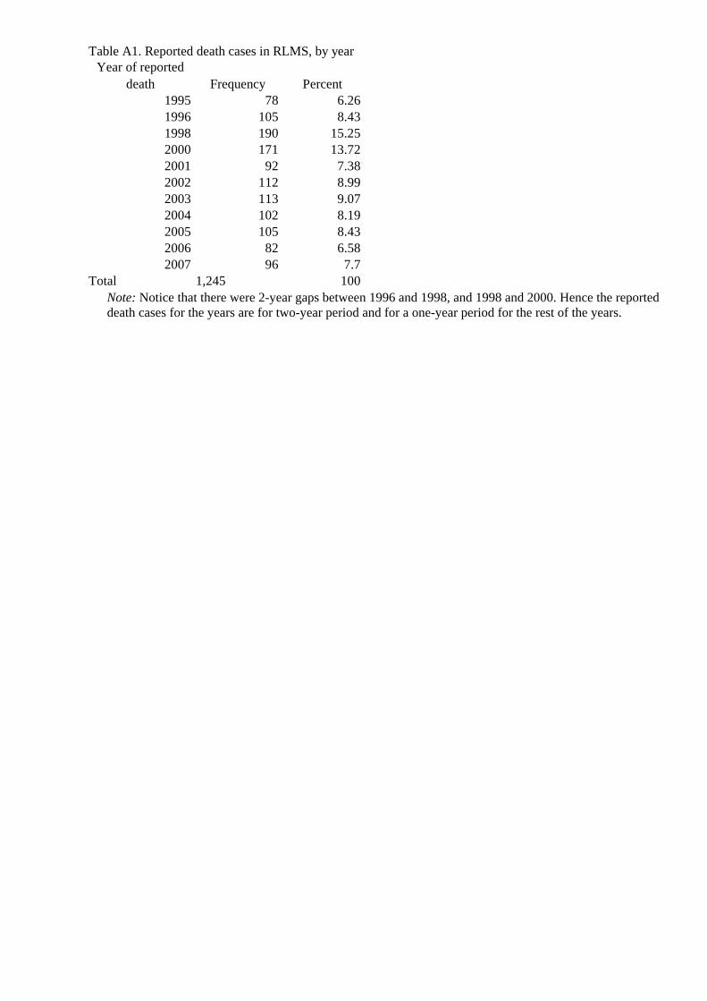
Year of reported death Frequency Percent

1995 78 6.261996 105 8.431998 190 15.252000 171 13.722001 92 7.382002 112 8.992003 113 9.072004 102 8.192005 105 8.432006 82 6.582007 96 7.7

Total 1,245 100

Table A1. Reported death cases in RLMS, by year

Note: Notice that there were 2-year gaps between 1996 and 1998, and 1998 and 2000. Hence the reported death cases for the years are for two-year period and for a one-year period for the rest of the years.

Table A2. Description of variables

Death event Death is reported to be the reason why [NAME AND PATRONYMIC] is no longer a member of a household

Married In a registered marriage

Smokes Smokes nowBinge drinker Used alcoholic beverages every day or 4-6 times a week in the last 30 days

Body mass index Weight/Height^2 based on height and weight reported in 'Medical measurement section'

Ever had a heart attack Have you ever been diagnosed with a “myocardial infarction”?

Ever had a stroke Has a doctor ever diagnosed you as having had a stroke--blood hemorrhage in the brain?

Diabetic Did a physician tell you at any time that you had diabetes or increased sugar in the blood?

Self-estimated health How would you evaluate your health? 1-very bad, …, 5-very good

Could not afford or find prescribed medicineThere were medicines prescribed or recommended in the last 30 days that you were not able to find or buy: had no money or could not find in pharmacy

Concern about getting necessities

How concerned are you about the possibility that you might not be able to provide yourself with the bare essentials in the next 12 months? Recoded from 1-5 scale into a binary scale: 1- very concerned and 0 otherwise

Experienced more than three movements in labor market or downward occupational mobility

Moved between work for wages, self-employment or entrepreneurship and non-employment and had more than three shifts OR experienced downward occupational mobility. The shifts are recorded on the basis of the job sections of adult questionnaire for each year

Consumption decile Decile based on per capita household expenditure in a year

Economic rank (1-the poorest, …, 9- the richest)Please imagine a nine-step ladder where on the bottom, the first step, stand the poorest people, and on the highest step, the ninth, stand the rich. On which step of the nine are you today?

Respect rank (1-the least respected, …, 9- the most respected)

And now another nine-step ladder where on the lowest step stand people who are absolutely not respected, and on the highest step stand those who are very respected. On which of the nine steps are you personally standing today?

Household in poverty

Household income is below absolute poverty rate. The poverty level is based on the minimum consumption basket and takes into account regional prices, demographic compostion of a household and economies of scales

Relative price of vodka to bread in locality Relative price of the lowest price of vodka to the price of white bread in a primary sample unit

Log vodka price in locality (in 1994 prices) Logarithm of the lowest price of vodka in a primary sample unit deflated to 1994 by annual CPI