Moral Hazard vs. Land Scarcity - The World Bank

Policy Research Working Paper 9012

Moral Hazard vs. Land Scarcity

Flood Management Policies for the Real World

Paolo AvnerStephane Hallegatte

Global Facility for Disaster Reduction and RecoverySeptember 2019

Pub

lic D

iscl

osur

e A

utho

rized

Pub

lic D

iscl

osur

e A

utho

rized

Pub

lic D

iscl

osur

e A

utho

rized

Pub

lic D

iscl

osur

e A

utho

rized

Produced by the Research Support Team

Abstract

The Policy Research Working Paper Series disseminates the findings of work in progress to encourage the exchange of ideas about development issues. An objective of the series is to get the findings out quickly, even if the presentations are less than fully polished. The papers carry the names of the authors and should be cited accordingly. The findings, interpretations, and conclusions expressed in this paper are entirely those of the authors. They do not necessarily represent the views of the International Bank for Reconstruction and Development/World Bank and its affiliated organizations, or those of the Executive Directors of the World Bank or the governments they represent.

Policy Research Working Paper 9012

This paper investigates the costs and benefits of three ex ante flood management strategies—risk-based insurance, zoning, and subsidized insurance—in an urban econom-ics framework that takes land scarcity into account. In a theoretical setting and in the absence of market failures, risk-based insurance perfectly internalizes flood risks and maximizes social welfare. However, risk-based insurance faces major technical, social, and political challenges and is not always realistic. Flood zoning and subsidized insurance are two second-best options that are easier to implement and less technically demanding. The paper explores ana-lytically and with numerical simulations the welfare losses and distributional impacts with these second-best options, and demonstrates that total losses often remain small. Flood zoning is close to optimal when flood-prone areas are small,

floods are frequent, and housing quality is low. Zoning keeps total land value unchanged but transfers wealth from landowners in flood-prone areas to landowners in safe locations. Subsidized insurance is close to optimal when a large fraction of a city is flood prone, floods are rare, and housing quality is high. And although it increases flood losses through the moral hazard effect, subsidized insurance encourages more construction, which reduces housing rents and benefits tenants regardless of where they live. Subsidized insurance transfers wealth from landowners in safe locations to landowners in flood-prone areas. When the implementation of risk-based insurance is unrealistic, as is often the case in developing countries, a combination of zoning in high-risk areas and subsidized insurance for low-risk areas might be a good alternative.

This paper is a product of the Global Facility for Disaster Reduction and Recovery. It is part of a larger effort by the World Bank to provide open access to its research and make a contribution to development policy discussions around the world. Policy Research Working Papers are also posted on the Web at http://www.worldbank.org/prwp. The authors may be contacted at [email protected].

MoralHazardvs.LandScarcity:FloodManagementPoliciesfortheRealWorld

Paolo Avner Stephane Hallegatte World Bank World Bank

JEL Codes: R14, R11, R13, C63, H21, H23, Q54,

Key words: Urban economics, urban floods, risk‐based insurance, land use zoning, subsidized

insurance, moral hazard, land scarcity

2

1. Introduction

Economic losses due to natural disasters – and especially floods – are increasing, mostly because of

increases in population and wealth in urban areas (Pielke et al. 2008; Neumayer and Barthel 2011;

Hallegatte 2017; Hoeppe 2016; Weinkle et al. 2018; Paprotny et al. 2018). Many have called for

resolute action to reduce flood losses (e.g., Kunreuther, Michel‐Kerjan, and Doherty 2011). But what

can governments do?

A first option is to do nothing, leaving affected people to pay for their own losses after a flood through

self‐insurance or a market insurance (Michel‐Kerjan and Kunreuther 2011). In that case, a national or

local government has nothing to do, beyond the provision of information about flood risks (Camerer

and Kunreuther 1989) and the regulation of insurance markets to ensure fair competition and

acceptable insurer bankruptcy risks. In theory, landowners and tenants would then include the cost of

floods into their decisions regarding the quality and robustness of building construction, the level of

rents, their localization choices, and the purchase of insurance. In the absence of market failures, this

solution leads to an optimal level of construction and of flood losses.

The real world is far from this ideal situation. A first issue is the low penetration of flood insurance that

is usually observed. This has two consequences. First, the insurance premium is one of the main

channels through which the risk of floods is internalized in housing prices (Speyrer and Ragas 1991;

Beltrán, Maddison, and Elliott 2018; Trond and Hofkes 2015; Bin, Kruse, and Landry 2008). In the

absence of insurance, housing prices tend to ignore flood risks. Second, in the absence of insurance,

affected people are usually in deep financial trouble after floods. In such a context, governments

usually have to step in and support the recovery of the population, for two main reasons. The first

reason is the widely accepted responsibility of governments to support people in times of crisis – it is

impossible for a government to ignore the situation of people who have lost their home or job in a

large disaster. Governments face a time consistency issue and a lack of ability to commit, as is well

known in monetary and fiscal policy (Kydland and Prescott 1977). The second reason is the externalities

linked to recovery and reconstruction. The inability of one family to recover and rebuild their home

has implications for the community: to ensure the sustainability of infrastructure networks and the

functioning of a community, people need to come back to the affected areas and rebuild, an issue

illustrated by the difficulty of rebuilding New Orleans’ neighborhoods after hurricane Katrina.

When governments provide post‐disaster support without having the systems in place before the

event, they often use ad hoc targeting and delivery mechanisms, which are expensive and lack

predictability, making it difficult for people to take into account this support in their decision making.

Also ad hoc post‐disaster support systems have been accused of creating a moral hazard, which in turn

reduces the take‐up of insurance contracts.

Another option for government is to mandate insurance against natural disasters, ensuring that

penetration reaches 100 percent. This option is however politically difficult, mostly because of

technical and political issues. The technical issues relate first to the difficulty in assessing the risk level

and therefore the appropriate risk‐based premium and second relate to enforcement issues, especially

in countries with weak tenure systems and administrative capacities. Political issues relate to the

heterogeneity in risk‐based premium and affordability issues. It is difficult for people to accept a

mandatory system that makes them pay an insurance premium that varies widely across

neighborhoods, based on models with large uncertainties. And the implementation of mandatory

3

insurance can have a strong impact on households who settled in flood‐prone areas (especially the

poorest who may have chosen this localization because this is where land prices are the lowest) (Lall

and Deichmann 2010; Michel‐Kerjan and Kunreuther 2011). While complementary policies or tax

breaks to help households cope with insurance costs have been proposed in rich countries (Kunreuther

(1996) and Picard (2008)), mandatory insurance remains politically challenging.

If neither the laissez‐faire approach nor the mandatory insurance system is desirable or possible, then

what are the other options? This paper explores two other second‐best policy instruments that are

implemented: flood zoning, i.e. a ban of construction in flood‐prone areas, and a subsidized insurance

system in which people have insurance but pay a premium that is independent of the risk level (with

cross‐subsidies from low‐risk to high‐risk households).

These options are not costless. Flood zoning diminishes the land available for construction, and

interacts with urbanization and land‐use management (Burby 2001; Burby et al. 2001; Lall and

Deichmann 2010). In a situation of land scarcity, which is the case in many cities and coastal areas, it

increases real estate pressure, possibly leading to increased rents and smaller dwellings for all

inhabitants.

A subsidized, mandatory insurance system can be financed from a local tax whose rate is independent

of the individual flood risk level. Such a scheme exists in France with the CAT‐NAT system (Grislain‐

Letrémy and Peinturier 2010). This option is also costly, as it creates moral hazard: households who

decide to settle in risk‐free areas have to pay for those who take more risks and benefit from these

risks (e.g., through an easier access to infrastructure or through amenities). This system thus subsidizes

risk‐taking behavior and may lead to larger flood losses (Laffont 1995).1

This paper investigates flood risks in an idealized city prone to flooding and provides a framework for

analyzing the relative costs and advantages of flood zoning, subsidized insurance, and risk‐based

market insurance, taking into account the impact of these policies on rent and housing affordability. It

builds on (Frame 2001) in that it combines a classical urban economic model (Alonso 1964; Mills 1967;

Muth 1969; Fujita 1989) with a simple representation of flood risks to investigate the efficiency of first‐

best and second‐best options in different contexts and for different floods. This paper adds to Frame

(2001) by investigating a fuller set of flood management policies, including in particular flood zoning in

the policy portfolio, and by modeling decisions regarding housing investments and density in flood and

safe areas.2 And this paper goes beyond the demonstration that subsidies can theoretically make sense

by quantifying the trade‐offs between efficiency and political acceptability and identifying conditions

that make the various policies particularly attractive in a specific city and to manage specific events.

The findings of the paper are as follows. First, as expected in the absence of market failures,

(actuarially‐fair) risk‐based premium insurance dominates other flood management strategies in terms

of household welfare irrespective of the characteristics of the floods (return period, flood prone area

and vulnerability of buildings and infrastructure). However, for most types of floods, the additional

cost of second‐best options (land use zoning or subsidized insurance) compared with the optimum is

1 Because of moral hazard, subsidized insurance is often completed with risk reduction measures (see Michel‐Kerjan and Kunreuther, 2011, on the National Flood Insurance Program in the U.S.). 2 Frame (2001) assumes that people consume land directly, without having to invest in building of different height and density. As a result, he cannot explore the effect of moral hazards when investments in building in flood zones are incentivized by subsidized insurance and is thus missing an essential component of the problem.

4

small, representing in most instances less than half a percentage point of income and in many cases

less than 0.2%. In particular, moral hazard does increase flood losses, but the effect remains limited

(and it could be limited further with appropriate deductibles). The difference between first and second‐

best options is smaller when floods are rare, flood affected areas are limited, and damages are low.

This distance increases for more frequent, larger in extent, and more damaging floods. If the subsidized

system has lower transaction costs than the risk‐based system (for instance because of the need to

assess risk at the plot level and to provide heterogeneous pricing), then the subsidized system could

dominate, especially in low‐risk environments.

Second, the preferred second‐best option (zoning or subsidized insurance) depends on the

characteristics of the floods. For frequent floods affecting a small share of the urban area, land use

zoning yields lower welfare losses than subsidized insurance. This is because the loss of land remains

moderate and does not significantly affect rents and housing affordability, while the effect of moral

hazard for frequent floods is large. For floods with larger extent, the impact of zoning on housing

affordability becomes significant and subsidized insurance dominates. Zoning also becomes preferable

when buildings and infrastructure are more vulnerable, which may be the case due to low quality

housing or due to flood characteristics (e.g., in places with flash floods that are particularly

destructive). This paper only considers economic losses, but the inclusion of (non‐insurable) human

losses would only reinforce these findings.

Finally, as already noted in (Frame 2001), the urban land markets play a key role in distributing the

costs and benefits of flood management policies across the population. The costs of zoning are

concentrated on the owners of the land that cannot be constructed, but an additional cost is imposed

to all tenants through increased rents (which benefit landowners in safe areas). And the benefits from

the subsidies in a subsidized insurance system are not fully captured by people living (or owning land)

in risky areas: the increased construction reduces rents, which benefits all tenants (at the expense of

people owning land in safe places). These distributed costs are small per capita and largely invisible

(and therefore disregarded in policy discussions), but the aggregate numbers can be large and play a

key role in explaining which policy dominates.

Taken together, these findings highlight the large distributional impacts of flood management, which

explain why implementation of such policies is challenging (World Bank 2013). They also suggest that

while risk‐based premium insurance is the preferable option if transaction costs are not too large,

there are other options that are easier to implement and more politically acceptable, and incur only a

small incremental aggregate cost. A combination of flood zoning (in high‐frequency low‐scale floods

and high‐vulnerability areas) and subsidized insurance (to manage rarer but large extent events) is

close to the optimal solution and much easier to implement both in political and practical terms. At

the core of these findings lies the trade‐off between limiting damages by reducing the housing capital

exposed to floods and reducing housing rents by increasing housing supply.

The paper is organized as follows. Section 2 presents the urban economy theory and our approach to

include flood risks. Then, Section 3 introduces the two insurance systems as well as the land use zoning

policy and provides analytical expressions of households’ welfare (and its income equivalent), the costs

of each policy and the impact on land rents. Section 4 provides a numerical assessment and ranks the

three systems for different characteristics of flood risks in the city. Section 5 concludes on the practical

application of these results.

5

2. Urban economic theory

2.1. Principles

In this section, we present the principal features and equations of the standard urban economic

modeling framework. We do so briefly, because it has been extensively described in many papers and

books (e.g., (Brueckner 2011; Fujita 1989)). We use a model inspired by von Thünen (1826), adapted

by Alonso (1964), Mills (1967), and Muth (1969) and comprehensively described in Fujita (1989).

Assuming that a city is defined by a number of jobs located in a single location, the CBD, this static

model is based on two trades‐offs, made by two categories of economic actors:

Households choose their housing location in the agglomeration by arbitrating between larger

and cheaper dwellings further from the city center, and increased commuting costs to the city

center where all jobs are assumed to be located.

Landowners choose where and how much to invest (i.e., what buildings to construct), as a

function of expected rents at each location.

These two trades‐offs characterize a static equilibrium in the urban system.

Table 1: Nomenclature

Symbol Signification

𝑅 Housing rents (or, equivalently, annualized real estate

price per square meter)

𝑅 Agricultural rent

𝐿 Available land for construction

𝐾 Invested capital

𝜌 Depreciation rate of capital

𝑖 Interest rate : cost of capital

𝛿 Fraction of damaged capital when a flood occurs

𝜏 𝑝 𝜃 𝑛 𝑞 𝑁 𝑟

Return time of a flood (i.e. the inverse of frequency) Unitary transport cost/km Share of flood prone areas in an agglomeration Household density Dwelling size Population in the agglomeration Limit of the city, maximum radius to the center

2.1.1. Households

Each household is composed of one representative worker living at a distance 𝑟 from the city business

district (CBD) where all jobs are located. Each worker has to commute once a day to the CBD, and this

commuting entails transportation costs 𝑇 𝑟 . All households are supposed to earn the same income 𝑌 and – at the equilibrium – they have the same level of satisfaction described by a utility function 𝑈

that depends on both the level of consumption of a composite good 𝑧 and of the size of their dwelling 𝑞. The level of rents per square meter (or, equivalently, the annualized real estate price per square

meter) is 𝑅 𝑟 , at each location in the city. Each household maximizes his or her utility function under

6

the budget constraint described in (1) by choosing where to settle in the urban area 𝑟, where 𝑟 is the distance to the CBD, how much housing space 𝑞 to consume and what to spend on other goods 𝑧. The term 𝐿 represents the annual amount accruing from land rents per household which is recycled in the

urban economy in the form of increased incomes.

𝑀𝑎𝑥 , , 𝑈 𝑧, 𝑞 𝑠. 𝑡. 𝑧 𝑅 𝑟 𝑞 𝑇 𝑟 𝑌 𝐿 (1)

2.1.2. Landowners

Landowners first decide whether to allocate land to agricultural purposes or to housing. In the first

case their revenue is 𝑅 𝐿, where 𝑅 is the agricultural rent and 𝐿 the area of land they own. In the second case, they choose what amount of capital 𝐾 𝑟 to invest at each distance from the CBD to

produce a housing surface 𝐻 𝑟 . In this framework, they are thus also the owners of the buildings. The

amount of floor space built and the annual land rents depend on an exogenous specific construction

technology which displays constant returns to scale but diminishing returns to capital: 𝐻 𝑟𝐹 𝐾 𝑟 , 𝐿 𝑟 . These decreasing returns to capital will cap the building heights and as consequence

the total amount of residential floor space. Developers will only invest large amounts of capital to build

tall buildings when the anticipated rents they expect will offset the extra building costs. The edge of

the city is given by an exogenous and constant agricultural rent 𝑅 below which it is no longer

profitable to build. At the edge of the city (𝑟 ) we therefore have 𝑅 𝑟 𝑅 . Landowners maximize

their profit function (2), which consists in identifying the optimal amount of capital to invest at each

location (3):

𝜋 𝑟 𝑅 𝑟 𝐹 𝐾 𝑟 , 𝐿 𝑟 𝑖 𝜌 𝐾 𝑟 (2)

𝐾 𝑟 𝐴𝑟𝑔𝑚𝑎𝑥 𝑅 𝑟 𝐹 𝐿 𝑟 , 𝐾 𝑟 𝜌 𝑖 𝐾 𝑟 (3)

The parameters 𝜌 and 𝑖 represent respectively the depreciation parameter of housing and the interest

rate. Together they constitute the unitary costs of capital.

The term 𝐿 found in (1) can schematically take on one of two values depending on the type of model

used: Closed City model with Absentee landowners (CCA) or Closed City model with Public ownership

of land (CCP). In the closed city model with absentee landowners (CCA), landowners are supposed to

live outside the urban area which means that land rents are not recycled in the local economy in the

form of increased incomes. In this case 𝐿 0. At the opposite end of the spectra, if all land plots are supposed to be owned by a local government (or by all households in equal shares) then 𝐿

𝑑𝑟, where 𝑁 is the number of households in the urban area.

2.2. Functional forms and equilibrium

We use Cobb‐Douglas functional forms with constant returns to define households’ utility and the

housing service construction function. This choice is widely shared in urban economics and makes it

possible to show analytically that there is both existence and uniqueness of an urban equilibrium (Mills

1972; Brueckner 1980; Fujita 1989):

𝑈 𝑧, 𝑞 𝑧 𝑞 𝑤ℎ𝑒𝑟𝑒 𝛼, 𝛽 0 𝑎𝑛𝑑 𝛼 𝛽 1 (4)

7

𝐹 𝐿, 𝐾 𝐴𝐿 𝐾 𝑤ℎ𝑒𝑟𝑒 𝑎, 𝑏 0 𝑎𝑛𝑑 𝑎 𝑏 1 (5)

We also make the following simplifying assumptions:

Transport costs increase linearly with distance from the city center, 𝑇 𝑟 𝑝𝑟, where p is the generalized cost of transportation including the cost of time.

The agricultural rent 𝑅 is supposed to be null. This simplification is not necessary but it makes

most of the calculations much easier without altering results.

At each distance 𝑟 from the city center, and assuming a perfectly circular city, we can define

the available land as the following increasing function of r: 𝐿 𝑟 𝑙𝑟 where 𝑙=2𝜋

This modeling framework is particularly well suited to study the costs and benefits of different flood‐

management strategies. Indeed, by informing on household utility, it enables us to quantify both the

monetary cost of floods and the disutility from reduced land availability, increased rents and smaller

dwelling sizes. It thus constitutes a comprehensive, although schematic, framework for flood

management policy evaluation.

2.3 Introducing floods in the urban economy model

We introduce floods in the traditional urban economy model, assuming that the only impact of floods

is through capital destruction. All other consequences (e.g., casualties and fatalities) are disregarded,

assuming they can be avoided with relevant tools, e.g., early warning and evacuation.3

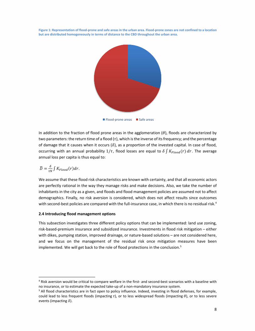
We consider that there are two zones in the agglomeration. One zone is flood prone and represents a

fraction 𝜃 of total available land; one zone is safe and represents a fraction 1 𝜃. The flood‐prone zones are not confined to a specific area in the city; instead, they are assumed to be distributed

homogeneously in terms of distance to the CBD throughout the agglomeration. One could picture this

situation as a disk, a slice of which is flood prone, such that flood prone areas and non‐flood prone

areas are in proportions 𝜃and 1 𝜃 (see Figure 1). In flood‐prone zones, the invested capital at each location in the city is noted 𝐾 𝑟 . Conversely, the invested capital in other parts of the city is

𝐾 𝑟 .

3 The fact that economic losses increase with income while the number of fatalities from natural disasters decreases with income (Kahn 2005) suggest that human losses can be reduced with other tools than economic losses.

8

Figure 1: Representation of flood‐prone and safe areas in the urban area. Flood‐prone zones are not confined to a location but are distributed homogeneously in terms of distance to the CBD throughout the urban area.

In addition to the fraction of flood prone areas in the agglomeration (𝜃), floods are characterized by two parameters: the return time of a flood (𝜏), which is the inverse of its frequency; and the percentage of damage that it causes when it occurs (𝛿), as a proportion of the invested capital. In case of flood, occurring with an annual probability 1/𝜏 , flood losses are equal to 𝛿 𝐾 𝑟 𝑑𝑟 . The average annual loss per capita is thus equal to:

𝐷 𝐾 𝑟 𝑑𝑟.

We assume that these flood risk characteristics are known with certainty, and that all economic actors

are perfectly rational in the way they manage risks and make decisions. Also, we take the number of

inhabitants in the city as a given, and floods and flood management policies are assumed not to affect

demographics. Finally, no risk aversion is considered, which does not affect results since outcomes

with second‐best policies are compared with the full‐insurance case, in which there is no residual risk.4

2.4 Introducing flood management options

This subsection investigates three different policy options that can be implemented: land use zoning,

risk‐based‐premium insurance and subsidized insurance. Investments in flood risk mitigation – either

with dikes, pumping station, improved drainage, or nature‐based solutions – are not considered here,

and we focus on the management of the residual risk once mitigation measures have been

implemented. We will get back to the role of flood protections in the conclusion.5

4 Risk aversion would be critical to compare welfare in the first‐ and second‐best scenarios with a baseline with no insurance, or to estimate the expected take‐up of a non‐mandatory insurance system. 5 All flood characteristics are in fact open to policy influence. Indeed, investing in flood defenses, for example, could lead to less frequent floods (impacting 𝜏), or to less widespread floods (impacting 𝜃), or to less severe events (impacting 𝛿).

Flood‐prone areas Safe areas

9

In the remaining of this paper, all variables are subscripted with a “𝑁” when a situation with no flood

is considered, with a “𝑃” when a situation with risk‐based premium insurance is considered, with a “𝑆” when a subsidized insurance is considered and finally with a “𝑍” when land use zoning is implemented.

2.4.1 Land use zoning

With land use zoning, developers are prevented from building in flood prone areas and can only

provide housing in safe areas.6 As a result of these restrictions, land available for construction is 𝐿1 𝜃 𝐿 and the installed capital, building on equation (3) corresponds to the following maximization:

𝐾 1 𝜃 𝐴𝑟𝑔𝑚𝑎𝑥 𝑅 𝐹 𝐿, 𝐾 𝜌 𝑖 𝐾

2.4.2 Subsidized insurance

With subsidized insurance, households contribute to an insurance fund through local taxes, and this

fund pays for all reconstruction needs after a flood. In that case, household funds – and not landowner

resources – are used for reconstruction. There is thus no price signal inciting landowners to construct

less in flood prone areas, as is the case in the French system or the NFIP system in the US (Michel‐

Kerjan and Kunreuther 2011). In that case, landowners do not account for flood risks and build an

amount KS according to the following expression:

𝐾 𝐴𝑟𝑔𝑚𝑎𝑥 𝑅 𝐹 𝐿, 𝐾 𝜌 𝑖 𝐾

This capital is distributed proportionally in the flood‐prone and flood‐risk land:

𝐾 𝜃 𝐾 ,

𝐾 1 𝜃 𝐾

With this flood management policy, the income of households is reduced by the tax that finances the

insurance scheme. This tax per household is equal to the average flood losses divided by the

population, i.e.:

𝐷𝛿

𝜏𝑁𝐾 𝑟 𝑑𝑟 𝜃

𝛿𝜏𝑁

𝐾 𝑟 𝑑𝑟

We can therefore consider that the stakeholders’ decisions (households and landowners) will be taken

on the basis of a reduced income for households: 𝑌 𝐿 𝐷 .

2.4.3 Risk-based insurance

Here, we assume that risk‐based insurance is paid by landowners, and that the premium is calculated

as a function of the risk level in the considered land lot, assuming an actuarially‐fair price with no

transaction cost.7 The premium is thus equal to the local annualized cost of floods, which depends on

the location and the cost of the building. On average, flood losses (or flood insurance costs) are thus

6 We consider that land use zoning is perfectly implemented. In many developing country cities, enforcing land use zoning is a major challenge. An extension of this work could investigate the consequences of partial enforcement. 7 If the insurance was paid by tenants, then it would translate into reduced rents, the final cost being paid equivalently by building owners.

10

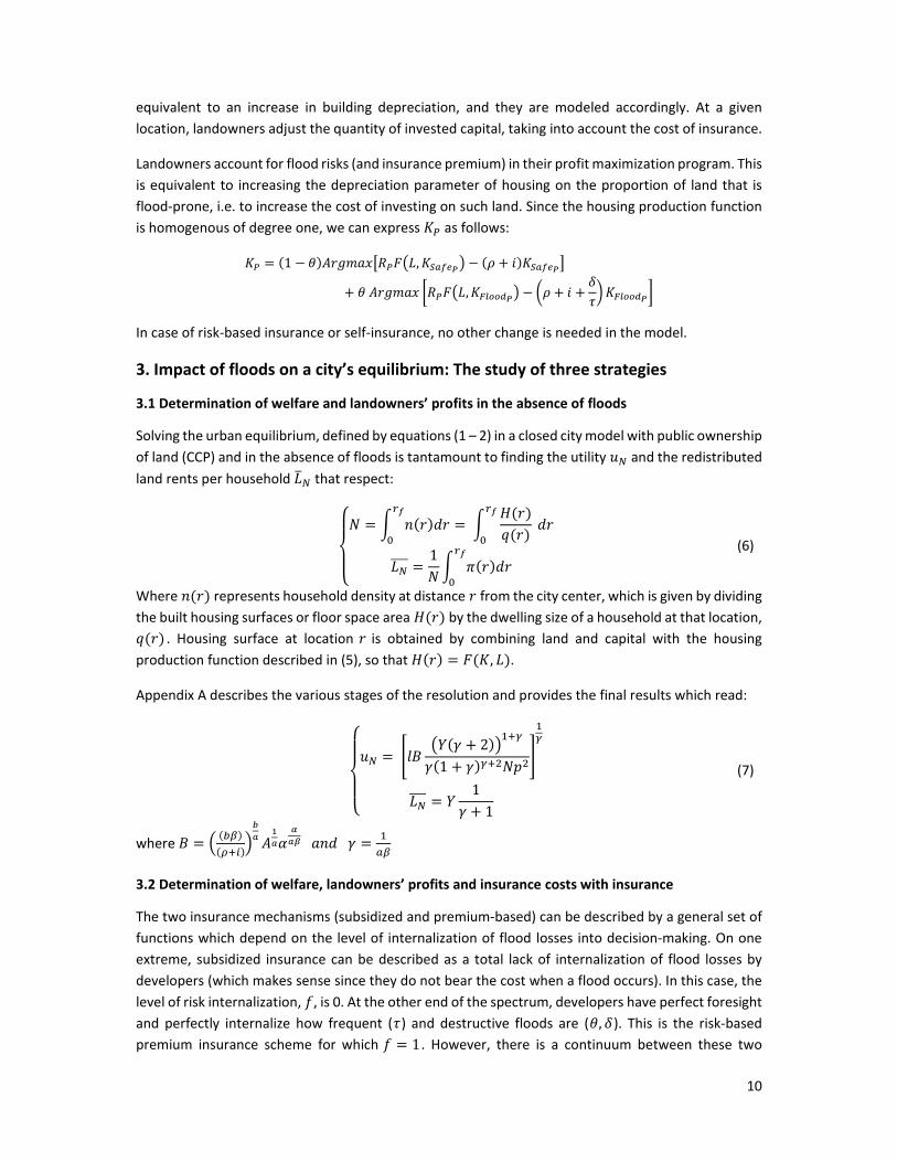
equivalent to an increase in building depreciation, and they are modeled accordingly. At a given

location, landowners adjust the quantity of invested capital, taking into account the cost of insurance.

Landowners account for flood risks (and insurance premium) in their profit maximization program. This

is equivalent to increasing the depreciation parameter of housing on the proportion of land that is

flood‐prone, i.e. to increase the cost of investing on such land. Since the housing production function

is homogenous of degree one, we can express 𝐾 as follows:


𝜃 𝐴𝑟𝑔𝑚𝑎𝑥 𝑅 𝐹 𝐿, 𝐾 𝜌 𝑖𝛿𝜏

𝐾

In case of risk‐based insurance or self‐insurance, no other change is needed in the model.

3. Impact of floods on a city’s equilibrium: The study of three strategies

3.1 Determination of welfare and landowners’ profits in the absence of floods

Solving the urban equilibrium, defined by equations (1 – 2) in a closed city model with public ownership

of land (CCP) and in the absence of floods is tantamount to finding the utility 𝑢 and the redistributed

land rents per household 𝐿 that respect:

⎩⎪⎨

⎪⎧𝑁 𝑛 𝑟 𝑑𝑟

𝐻 𝑟𝑞 𝑟

𝑑𝑟

𝐿1𝑁

𝜋 𝑟 𝑑𝑟 (6)

Where 𝑛 𝑟 represents household density at distance 𝑟 from the city center, which is given by dividing

the built housing surfaces or floor space area 𝐻 𝑟 by the dwelling size of a household at that location,

𝑞 𝑟 . Housing surface at location 𝑟 is obtained by combining land and capital with the housing

production function described in (5), so that 𝐻 𝑟 𝐹 𝐾, 𝐿 .

Appendix A describes the various stages of the resolution and provides the final results which read:

⎩⎪⎨

⎪⎧

𝑢 𝑙𝐵𝑌 𝛾 2

𝛾 1 𝛾 𝑁𝑝

𝐿 𝑌1

𝛾 1

(7)

where 𝐵 𝐴 𝛼 𝑎𝑛𝑑 𝛾

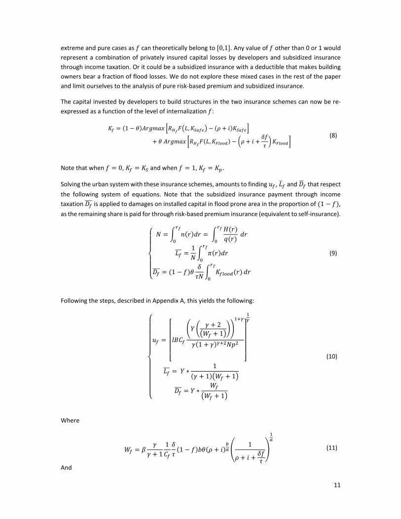
3.2 Determination of welfare, landowners’ profits and insurance costs with insurance

The two insurance mechanisms (subsidized and premium‐based) can be described by a general set of

functions which depend on the level of internalization of flood losses into decision‐making. On one

extreme, subsidized insurance can be described as a total lack of internalization of flood losses by

developers (which makes sense since they do not bear the cost when a flood occurs). In this case, the

level of risk internalization, 𝑓, is 0. At the other end of the spectrum, developers have perfect foresight

and perfectly internalize how frequent (𝜏) and destructive floods are (𝜃, 𝛿). This is the risk‐based premium insurance scheme for which 𝑓 1. However, there is a continuum between these two

11

extreme and pure cases as 𝑓 can theoretically belong to 0,1 . Any value of 𝑓 other than 0 or 1 would represent a combination of privately insured capital losses by developers and subsidized insurance

through income taxation. Or it could be a subsidized insurance with a deductible that makes building

owners bear a fraction of flood losses. We do not explore these mixed cases in the rest of the paper

and limit ourselves to the analysis of pure risk‐based premium and subsidized insurance.

The capital invested by developers to build structures in the two insurance schemes can now be re‐

expressed as a function of the level of internalization 𝑓:


𝜃 𝐴𝑟𝑔𝑚𝑎𝑥 𝑅 𝐹 𝐿, 𝐾 𝜌 𝑖𝛿𝑓𝜏

𝐾 (8)

Note that when 𝑓 0, 𝐾 𝐾 and when 𝑓 1, 𝐾 𝐾 .

Solving the urban system with these insurance schemes, amounts to finding 𝑢 , 𝐿 and 𝐷 that respect

the following system of equations. Note that the subsidized insurance payment through income

taxation 𝐷 is applied to damages on installed capital in flood prone area in the proportion of 1 𝑓 ,

as the remaining share is paid for through risk‐based premium insurance (equivalent to self‐insurance).

⎩⎪⎪⎨

⎪⎪⎧ 𝑁 𝑛 𝑟 𝑑𝑟

𝐻 𝑟𝑞 𝑟

𝑑𝑟

𝐿1𝑁

𝜋 𝑟 𝑑𝑟

𝐷 1 𝑓 𝜃𝛿

𝜏𝑁𝐾 𝑟 𝑑𝑟

(9)

Following the steps, described in Appendix A, this yields the following:

⎩⎪⎪⎪⎪⎨

⎪⎪⎪⎪⎧

𝑢

⎣⎢⎢⎢⎢⎡

𝑙𝐵𝐶

𝑌𝛾 2

𝑊 1


⎦⎥⎥⎥⎥⎤

𝐿 𝑌 ∗1

𝛾 1 𝑊 1

𝐷 𝑌 ∗𝑊

𝑊 1

(10)

Where

𝑊 𝛽𝛾

𝛾 11𝐶

𝛿𝜏

1 𝑓 𝑏𝜃 𝜌 𝑖1

𝜌 𝑖𝛿𝑓𝜏

(11)

And

12

𝐶 1 𝜃 𝜃𝜌 𝑖

𝜌 𝑖𝛿𝑓𝜏

(12)

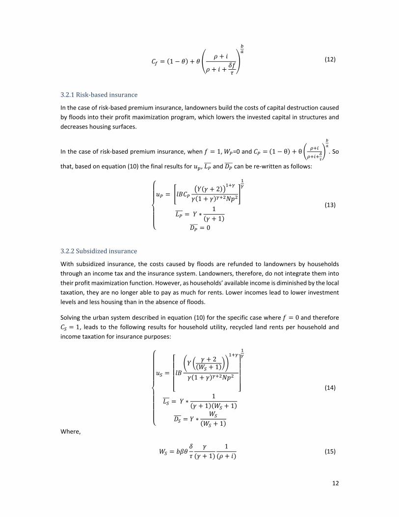
3.2.1 Risk-based insurance

In the case of risk‐based premium insurance, landowners build the costs of capital destruction caused

by floods into their profit maximization program, which lowers the invested capital in structures and

decreases housing surfaces.

In the case of risk‐based premium insurance, when 𝑓 1, 𝑊 =0 and 𝐶 1 θ θ . So

that, based on equation (10) the final results for 𝑢 , 𝐿 and 𝐷 can be re‐written as follows:

⎩⎪⎪⎨

⎪⎪⎧

𝑢 𝑙𝐵𝐶𝑌 𝛾 2


𝐿 𝑌 ∗1

𝛾 1𝐷 0

(13)

3.2.2 Subsidized insurance

With subsidized insurance, the costs caused by floods are refunded to landowners by households

through an income tax and the insurance system. Landowners, therefore, do not integrate them into

their profit maximization function. However, as households’ available income is diminished by the local

taxation, they are no longer able to pay as much for rents. Lower incomes lead to lower investment

levels and less housing than in the absence of floods.

Solving the urban system described in equation (10) for the specific case where 𝑓 0 and therefore 𝐶 1, leads to the following results for household utility, recycled land rents per household and income taxation for insurance purposes:

⎩⎪⎪⎪⎨

⎪⎪⎪⎧

𝑢

⎣⎢⎢⎢⎡

𝑙𝐵𝑌

𝛾 2𝑊 1


⎦⎥⎥⎥⎤

𝐿 𝑌 ∗1

𝛾 1 𝑊 1

𝐷 𝑌 ∗𝑊

𝑊 1

(14)

Where,

𝑊 𝑏𝛽𝜃

𝛿𝜏

𝛾𝛾 1

1𝜌 𝑖

(15)

13

3.3 Determination of welfare and landowners’ profits with land use zoning

In the case of land use zoning, finding the urban equilibrium is similar to a case where there are no

floods in the city, 𝑁, but with reduced availability of land. There are no insurance schemes, so that

income is not taxed and the depreciation rate of capital is similar to a no‐flood situation. The urban

equilibrium in the case of zoning is found when the following system of two equations is verified.

⎩⎪⎨

⎪⎧𝑁 𝑛 𝑟 𝑑𝑟

𝐻 𝑟𝑞 𝑟

𝑑𝑟 𝐹 𝜃𝐿, 𝐾

𝑞 𝑟 𝑑𝑟

𝐿1𝑁

𝜋 𝑟 𝑑𝑟 (16)

Solving this system yields the following results for household utility and recycled land rents per

household.

⎩⎪⎨

⎪⎧

𝑢 𝑙𝐵 1 𝜃𝑌 𝛾 2


𝐿 𝑌1

𝛾 1

(17)

3.4 Comparing outcomes for the three flood management strategies

This section compares the results for the three flood management strategies land use zoning, risk‐

based premium insurance and subsidized insurance. Whereas the main variable that we are concerned

with is the representative household’s utility in each case, it is also informative to explore the possible

distributional impacts by looking at landowners’ land rents and tenants’ rents and housing costs.

3.4.1 Land rents for each flood management strategy

The land rents per household in equations (7), (13), (14) and (17) provide the basis for the comparison.

The first striking observation is that although land available for buildings, the level of invested capital

into structures and housing surfaces are lower with land use zoning (𝑍) and risk‐based premium

insurance (𝑃) compared to a situation without floods (𝑁), total land rents and land rents per capita (𝐿) are identical.

𝐿 𝐿 𝐿 𝑌 ∗1

𝛾 1

By comparison land rents in the subsidized insurance case are lower. This comes naturally from the

below equation, as , given that 𝑊 0.

𝐿 𝑌 ∗1

𝛾 1 𝑊 1𝐿 , ,

When land or capital for housing is lower, the market adjusts by increasing rents in the urban area.

This compensates the lack of housing floor space and leaves landowners’ profits unaffected. However,

in the subsidized insurance case, the subsidy paid by each household decreases the amount of income

14

that is available for housing expenditure, which in turn depresses housing rents and ultimately land

rents.

3.4.2 Household utility comparison

Ultimately, the best description of households’ welfare under the three flood management strategies

is the level of utility achieved. Since the landowners’ revenues are reintroduced as an additional

income of the city inhabitants, our model is equivalent to the ‘public ownership of land’ model. In this

case, Closed City model with Public ownership of land, Fujita demonstrate that the equilibrium which

maximizes household utility is also the optimal outcome that maximizes the surplus of the Herbert‐

Stevens model (Fujita 1989, 63–75). 8

This implies that the scenarios with zoning or subsidized insurance achieve a lower utility than the

scenario with risk‐based premium insurance. Indeed, the scenario with zoning reduces the housing

capital compared with the optimum and therefore leads to a lower utility. Similarly, the scenario with

subsidized flood insurance has an externality since the actual depreciation rate in the flood zone is not

the one used in the optimization program of landowners. It leads to a housing capital that is strictly

larger in the flood zone than the housing capital in the optimal (non‐subsidized) case, and therefore to

a lower utility.

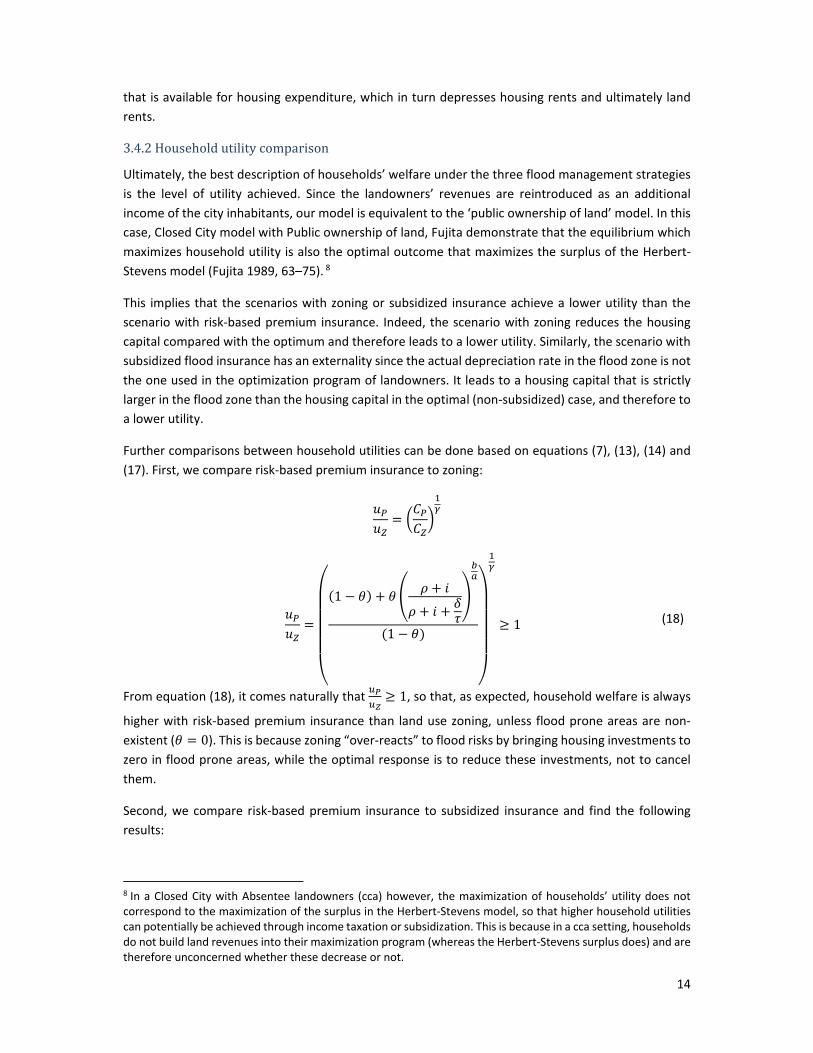
Further comparisons between household utilities can be done based on equations (7), (13), (14) and

(17). First, we compare risk‐based premium insurance to zoning:

𝑢𝑢

𝐶𝐶

𝑢𝑢

⎝

⎜⎜⎜⎜⎛ 1 𝜃 𝜃

𝜌 𝑖

𝜌 𝑖𝛿𝜏

1 𝜃

⎠

⎟⎟⎟⎟⎞

1 (18)

From equation (18), it comes naturally that 1, so that, as expected, household welfare is always

higher with risk‐based premium insurance than land use zoning, unless flood prone areas are non‐

existent (𝜃 0). This is because zoning “over‐reacts” to flood risks by bringing housing investments to

zero in flood prone areas, while the optimal response is to reduce these investments, not to cancel

them.

Second, we compare risk‐based premium insurance to subsidized insurance and find the following

results:

8 In a Closed City with Absentee landowners (cca) however, the maximization of households’ utility does not correspond to the maximization of the surplus in the Herbert‐Stevens model, so that higher household utilities can potentially be achieved through income taxation or subsidization. This is because in a cca setting, households do not build land revenues into their maximization program (whereas the Herbert‐Stevens surplus does) and are therefore unconcerned whether these decrease or not.

15

𝑢𝑢

𝐶 𝑊 1 (19)

Here, we know that since the model with perfect insurance fully internalizes the cost of floods through

the depreciation rate, it maximizes the utility, so that 1. However, this inequality is not obvious

in equation (19), since the full impact of the subsidy is the sum of two channels: the reduction in

welfare due to the higher cost of floods that is shared among all inhabitants; and the increase in

welfare due to higher housing supply. The first element in equation (19), 𝐶 , is positive but inferior or

equal to 1. The second member of the equation however is superior to 1.

So far, we have confirmed that the first‐best solution dominates. Now, we can compare the two

second‐best options, i.e. the subsidized insurance and land use zoning:

𝑢𝑢

1𝐶

𝑊 11

1 𝜃𝑊 1 (20)

The comparison of subsidized and land use zoning utilities is ambiguous, showing that theoretically

flood zoning or subsidized insurance could be the preferred second‐best policy. It is only easy to see

that when 𝜃 approaches one (the whole city is in a flood zone), then subsidized insurance dominates

zoning. In Section 4, we will turn to numerical simulations to explore the conditions under which one

of these second‐best solutions dominates.

To do so, we first define the “equivalent income” in each scenario. Indeed, the utility level is an abstract

construction and the differences in utility levels achieved between flood management options are hard

to interpret. For this reason, we translate utility differences in terms of income equivalents. In practice,

we identify the levels of income that would be required in the subsidized insurance and land use zoning

cases to achieve the same utility as in the risk‐based premium insurance setting. This amounts to

finding 𝑌 and 𝑌 such that 𝑈 𝑌 𝑈 𝑌 𝑈 𝑌 𝑢 .

First, we show in equation (21) the income equivalent needed for the utility with the subsidized

insurance to be equal to the utility level with risk‐based premium insurance. Note that, since we know

that utility is lower with the subsidy, we also know that 𝑌 is higher than 𝑌.

𝑈 𝑌 𝑢

⇔ 𝑌 𝑌𝐶 𝑊 1 (21)

Second, we show in equation (22) the income equivalent needed for the utility with land use zoning to

be equal to the utility level with risk‐based premium insurance. In this case 𝑌 is superior to 𝑌, which means that an increase in income would be needed with land use zoning for households to achieve

the same utility as with risk‐based premium insurance.

𝑈 𝑌 𝑢

⇔ 𝑌 𝑌𝐶𝐶

(22)

16

4. Numerical results

To explore how these theoretical results can inform decision‐making, we now rely on numerical

exercises. We calibrate an idealized city on the characteristics of the Paris agglomeration (in terms of

transport speed and cost, urban density, population, income, etc. see Appendix C) but a similar

exercise could easily be performed for different cities.

Then, we explore how the different policies perform with various values of flood parameters. In

particular, we consider cases in which the idealized city is exposed to frequent or rare floods, looking

at return periods ranging from one year to 50 years9 (for instance because the city has flood protection

to the corresponding standard). We also explore cases where the flood zones represent a small or a

large fraction of land, with flood‐prone areas ranging from 1 percent to 100 percent of the city area.

Finally, we explore for varying degrees of damage inflicted by floods. This is expressed through the

percentage of buildings construction value destroyed in flood prone areas when a flood occurs. We

represent cases where floods are nearly harmless, for example because they are only constituted by a

couple centimeters of water, to very damaging floods. The range of damage is 1% to 100% of buildings’

construction value.10

The real Paris agglomeration would be a situation with rare floods (with a return period of 50 to 100

years) and a relatively small area at risk (around 20 percent). A city like New Orleans would be exposed

to rare floods (the current protection system is supposed to protect the city against the 100‐year

hurricane at least), but with a large fraction of the city at risk (Katrina flooded 80 percent of the city).

And a city like Dar es Salam or Mumbai would be cases in which floods are very frequent (these cities

experience floods almost every year), but with a relatively small flooded area.

With the model presented in the previous section, we explore how risk‐based insurance, subsidized

insurance, and flood zoning perform in these different situations (keeping the socioeconomic

characteristics of the city constant).

4.1 Trade‐off between damages from floods and housing costs

The most common argument against subsidized insurance is that it creates moral hazard by

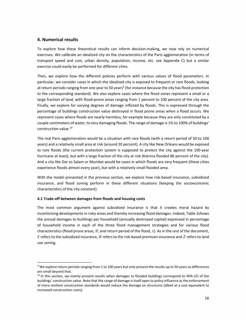
incentivizing developments in risky areas and thereby increasing flood damages. Indeed, Table 2shows

the annual damages to buildings per household (annually destroyed capital) expressed in percentage

of household income in each of the three flood management strategies and for various flood

characteristics (flood prone areas, 𝜃, and return period of the flood, 𝜏). As in the rest of the document,

𝑆 refers to the subsidized insurance, 𝑅 refers to the risk‐based premium insurance and 𝑍 refers to land use zoning.

9 We explore return periods ranging from 1 to 100 years but only present the results up to 50 years as differences are small beyond that. 10 In this section, we mainly present results when damages to flooded buildings correspond to 40% (𝛿) of the buildings’ construction value. Note that the range of damage is itself open to policy influence as the enforcement of more resilient construction standards would reduce the damage on structures (albeit at a cost equivalent to increased construction costs).

17

Flood zoning is associated to zero damages as the policy simply forbids construction in flood prone

areas. But subsidized insurance is associated with (much) higher annual damages per household than

the risk‐based premium insurance. This is because landowners and developers do not bear the cost of

flood risks and therefore build much more in the flood‐prone area, leading to large losses. Even with

relatively rare floods – with a 20‐year return period – flood losses are more than doubled in the

subsidized insurance case, compared with risk‐based insurance. The increase is even larger for more

frequent floods. These results confirm the importance of the moral hazard effect in the model.11

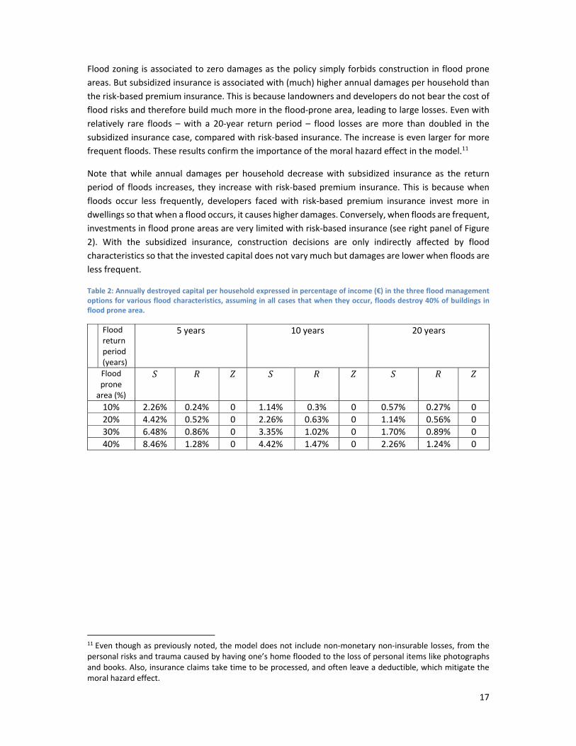
Note that while annual damages per household decrease with subsidized insurance as the return

period of floods increases, they increase with risk‐based premium insurance. This is because when

floods occur less frequently, developers faced with risk‐based premium insurance invest more in

dwellings so that when a flood occurs, it causes higher damages. Conversely, when floods are frequent,

investments in flood prone areas are very limited with risk‐based insurance (see right panel of Figure

2). With the subsidized insurance, construction decisions are only indirectly affected by flood

characteristics so that the invested capital does not vary much but damages are lower when floods are

less frequent.

Table 2: Annually destroyed capital per household expressed in percentage of income (€) in the three flood management options for various flood characteristics, assuming in all cases that when they occur, floods destroy 40% of buildings in flood prone area.

Flood return period (years)

5 years 10 years 20 years

Flood prone area (%)

𝑆 𝑅 𝑍 𝑆 𝑅 𝑍 𝑆 𝑅 𝑍

10% 2.26% 0.24% 0 1.14% 0.3% 0 0.57% 0.27% 0

20% 4.42% 0.52% 0 2.26% 0.63% 0 1.14% 0.56% 0

30% 6.48% 0.86% 0 3.35% 1.02% 0 1.70% 0.89% 0

40% 8.46% 1.28% 0 4.42% 1.47% 0 2.26% 1.24% 0

11 Even though as previously noted, the model does not include non‐monetary non‐insurable losses, from the personal risks and trauma caused by having one’s home flooded to the loss of personal items like photographs and books. Also, insurance claims take time to be processed, and often leave a deductible, which mitigate the moral hazard effect.

18

Figure 2: Invested capital density in safe (left) and flood prone areas (right) as a function of the distance to the city center with the three flood management options. In this example, floods occur every 5 years (𝝉), impacting 20% of the urban land area (𝜽) and destroying 40% of the buildings (𝜹).

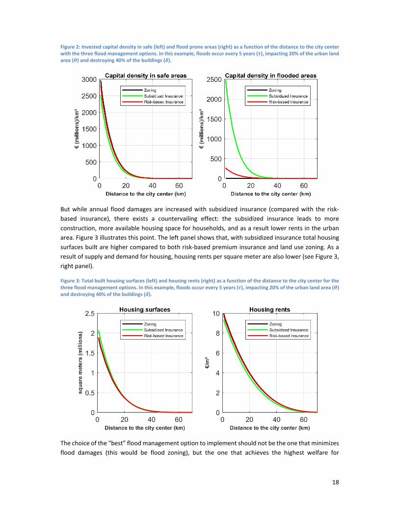
But while annual flood damages are increased with subsidized insurance (compared with the risk‐

based insurance), there exists a countervailing effect: the subsidized insurance leads to more

construction, more available housing space for households, and as a result lower rents in the urban

area. Figure 3 illustrates this point. The left panel shows that, with subsidized insurance total housing

surfaces built are higher compared to both risk‐based premium insurance and land use zoning. As a

result of supply and demand for housing, housing rents per square meter are also lower (see Figure 3,

right panel).

Figure 3: Total built housing surfaces (left) and housing rents (right) as a function of the distance to the city center for the three flood management options. In this example, floods occur every 5 years (𝝉), impacting 20% of the urban land area (𝜽) and destroying 40% of the buildings (𝜹).

The choice of the “best” flood management option to implement should not be the one that minimizes

flood damages (this would be flood zoning), but the one that achieves the highest welfare for

19

households. At the core of this reframed question, is the acknowledgment that there is a trade‐off in

urban areas between minimizing damages and lowering housing costs.

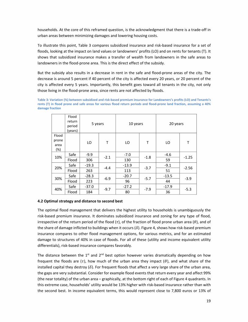
To illustrate this point, Table 3 compares subsidized insurance and risk‐based insurance for a set of

floods, looking at the impact on land values or landowners’ profits (LO) and on rents for tenants (T). It

shows that subsidized insurance makes a transfer of wealth from landowners in the safe areas to

landowners in the flood‐prone area. This is the direct effect of the subsidy.

But the subsidy also results in a decrease in rent in the safe and flood‐prone areas of the city. The

decrease is around 5 percent if 40 percent of the city is affected every 20 years, or 20 percent of the

city is affected every 5 years. Importantly, this benefit goes toward all tenants in the city, not only

those living in the flood‐prone area, since rents are not affected by floods.

Table 3: Variation (%) between subsidized and risk‐based premium insurance for Landowners’s profits (LO) and Tenants’s rents (T) in flood prone and safe areas for various flood return periods and flood‐prone land fraction, assuming a 40% damage fraction

Flood return period (years)

5 years 10 years 20 years

Flood prone area (%)

LO T LO T LO T

10% Safe ‐9.9

‐2.1 ‐7.0

‐1.8 ‐4.6

‐1.25 Flood 306 130 59

20% Safe ‐19.3

‐4.4 ‐13.9

‐3.7 ‐9.1

‐2.56 Flood 263 113 51

30% Safe ‐28.3

‐6.9 ‐20.7

‐5.7 ‐13.5

‐3.9 Flood 223 96 44

40% Safe ‐37.0

‐9.7 ‐27.2

‐7.9 ‐17.9

‐5.3 Flood 184 80 36

4.2 Optimal strategy and distance to second best

The optimal flood management that delivers the highest utility to households is unambiguously the

risk‐based premium insurance. It dominates subsidized insurance and zoning for any type of flood,

irrespective of the return period of the flood (𝜏), of the fraction of flood prone urban area (𝜃), and of the share of damage inflicted to buildings when it occurs (𝛿). Figure 4, shows how risk‐based premium

insurance compares to other flood management options, for various metrics, and for an estimated

damage to structures of 40% in case of floods. For all of these (utility and income equivalent utility

differentials), risk‐based insurance compares favorably.

The distance between the 1st and 2nd best option however varies dramatically depending on how

frequent the floods are (𝜏), how much of the urban area they impact (𝜃), and what share of the installed capital they destroy (𝛿). For frequent floods that affect a very large share of the urban area, the gaps are very substantial. Consider for example flood events that return every year and affect 99%

(the near totality) of the urban area – graphically, at the bottom right of each of Figure 4 quadrants. In

this extreme case, households’ utility would be 13% higher with risk‐based insurance rather than with

the second best. In income equivalent terms, this would represent close to 7,800 euros or 13% of

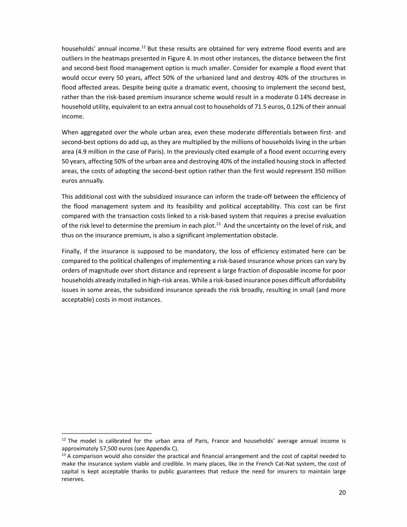
20

households’ annual income.12 But these results are obtained for very extreme flood events and are

outliers in the heatmaps presented in Figure 4. In most other instances, the distance between the first

and second‐best flood management option is much smaller. Consider for example a flood event that

would occur every 50 years, affect 50% of the urbanized land and destroy 40% of the structures in

flood affected areas. Despite being quite a dramatic event, choosing to implement the second best,

rather than the risk‐based premium insurance scheme would result in a moderate 0.14% decrease in

household utility, equivalent to an extra annual cost to households of 71.5 euros, 0.12% of their annual

income.

When aggregated over the whole urban area, even these moderate differentials between first‐ and

second‐best options do add up, as they are multiplied by the millions of households living in the urban

area (4.9 million in the case of Paris). In the previously cited example of a flood event occurring every

50 years, affecting 50% of the urban area and destroying 40% of the installed housing stock in affected

areas, the costs of adopting the second‐best option rather than the first would represent 350 million

euros annually.

This additional cost with the subsidized insurance can inform the trade‐off between the efficiency of

the flood management system and its feasibility and political acceptability. This cost can be first

compared with the transaction costs linked to a risk‐based system that requires a precise evaluation

of the risk level to determine the premium in each plot.13 And the uncertainty on the level of risk, and

thus on the insurance premium, is also a significant implementation obstacle.

Finally, if the insurance is supposed to be mandatory, the loss of efficiency estimated here can be

compared to the political challenges of implementing a risk‐based insurance whose prices can vary by

orders of magnitude over short distance and represent a large fraction of disposable income for poor

households already installed in high‐risk areas. While a risk‐based insurance poses difficult affordability

issues in some areas, the subsidized insurance spreads the risk broadly, resulting in small (and more

acceptable) costs in most instances.

12 The model is calibrated for the urban area of Paris, France and households’ average annual income is approximately 57,500 euros (see Appendix C). 13 A comparison would also consider the practical and financial arrangement and the cost of capital needed to make the insurance system viable and credible. In many places, like in the French Cat‐Nat system, the cost of capital is kept acceptable thanks to public guarantees that reduce the need for insurers to maintain large reserves.

21

Figure 4: Comparing risk‐based premium insurance to other flood management options for an estimated damage to buildings of 40%. Top left: as a % of household utility; Top right: as a % of household income; Bottom left: as income equivalent for households in monetary terms; Bottom right: as total income equivalent when aggregated over the whole urban area.

22

4.3 What is the second‐best option?

Assuming a risk‐based insurance system cannot be implemented for practical or political reasons, this

section explores which option between zoning and a universal subsidized insurance scheme would

entail the less welfare losses for a variety of flood events.

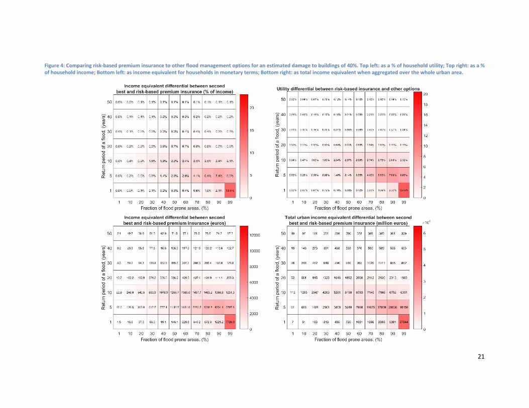
Figure 5 shows that the 2nd best option to mitigate the costs of floods on households’ welfare depends

on flood characteristics. For frequent floods, those that have a low return period, flood zoning would

lead to higher utility levels for households than the implementation of a subsidized insurance. This is

especially true for floods that affect a small fraction of total urban land. As the fraction of flood prone

area grows in cities, the cost of implementing zoning increases relative to subsidized insurance because

the land scarcity created by the policy increases housing costs.

Conversely for less frequent floods, subsidized insurance performs better than flood zoning. This result

translates the high costs of preventing construction in flood prone areas when floods occur rarely –

this cost manifests itself through the housing and land markets in the form of increased rents. In this

case subsidizing risk taking, in the form of construction in risky areas, has the benefit of reducing the

housing supply constraints and leads to lower unitary costs of housing that more than compensates

the destructions when floods occur.

Figure 5: Subsidized insurance and land use zoning each lead to higher household utilities depending on flood characteristics.

The costs of flood zoning only depend on how stringent the policy is; in other words, on what share of

the land is construction banned, or what share of land is located in flood prone areas. It is otherwise

independent from flood characteristics such as the damage caused by floods when they occur, or the

return period of the flood. This is because the costs of zoning are entirely linked to land scarcity and

the increased housing costs it entails, as, when applied appropriately, no damages occur once floods

23

hit. On the other hand, the welfare costs of implementing subsidized insurance depend on flood

characteristics and increase with the damages that floods cause. Subsidized insurance is therefore

costlier as flood damages increase, whereas zoning costs remain the same irrespective of flood

damages. For this reason, the number and type of events for which zoning is a better option than

subsidized insurance increase with the share of damage inflicted to buildings. This is graphically

captured in Figure 5 by the black area expanding on the grey area when flood damages increase from

30% to 50% of the costs of buildings.

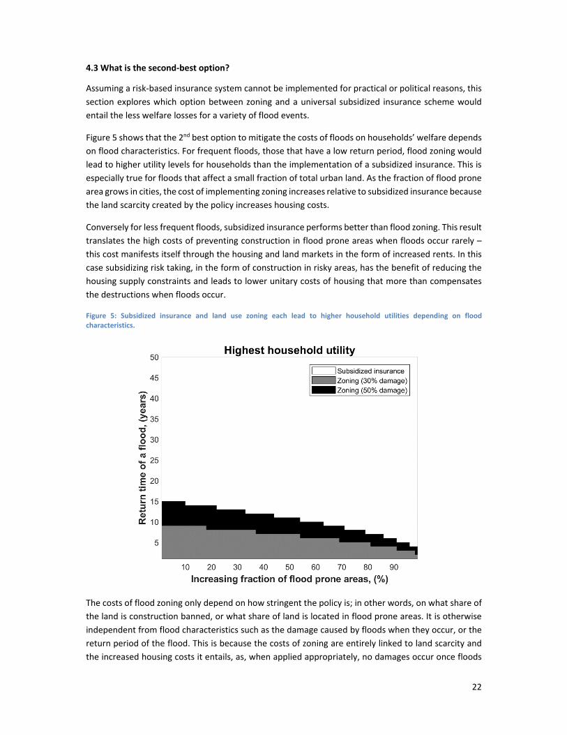
Figure 6: Households’ utility variation between subsidized insurance and land use zoning for flood event that destroy 40% of structures in flood‐prone areas.

Figure 6 complements Figure 5 as it provides variations in household’s utility when the subsidized

insurance is implemented by local decision makers rather than flood zoning. (In this case, risk‐based

insurance is not considered.) Green shades represent situations in which zoning is the preferable

option whereas for red shades, the best option is subsidized insurance. The color scheme matches the

information from Figure 5 but goes one step further, by informing on the magnitude of utility

differentials. What is striking is how large the variations in households’ utility can be, especially when

compared to the variation in utility between first‐ and second‐best options reported in the top left

quadrant of Figure 4. For large areas of Figure 6, variations in utility are at or above 2% and can reach

‐42% and +38%. This figure therefore shows that the costs of not implementing the correct second‐

best option when the first best is unavailable are very high.

The figure also highlights the cost of flood zoning when large areas are concerned: while flood zoning

is often considered as a “costless” measure, its impact on land scarcity and housing costs can be

significant and lead to large welfare losses for the population. Our results suggest that flood zoning

makes sense only for floods that are very frequent (with a return period at or below 5 years), and only

if there is no other option to prevent these floods, for instance with improved drainage or river dikes.

24

For rarer floods, it is preferable to provide a subsidized insurance contract to people living in the flood

zone than to prevent them from living here: the additional cost from floods is more than compensated

by the benefits from reduced land scarcity.

5. Conclusions

We use the standard urban economics model to characterize housing investment choices, utility

throughout the city, rents and dwelling sizes, in an agglomeration where a fraction of land is flood

prone. This theoretical framework is well suited for the study of flood costs and flood‐management

policy costs in an urban context. It enables to capture flood capital losses (i.e., housing capital

destruction), indirect costs (rent‐related losses and insurance costs), and the variation of landowners’

aggregated profits, assuming that other losses (e.g., human and cultural losses) can be avoided. Going

beyond the sole direct costs has the advantage of providing more comprehensive insights from a social

welfare perspective.

The results have relevant policy implications. First, except in extreme cases with large and frequent

floods, the difference in efficiency between a perfect risk‐based insurance system and a subsidized

insurance system with uniform premiums is small. Considering the challenges to implement a risk‐

based system, this result suggests that it makes sense in most places in the world to implement a

subsidized uniform system, at least as a first step. The efficiency cost due to the subsidy is small

because the moral hazard that causes an increase in flood losses is largely compensated by the benefits

from reduced housing scarcity and lower housing costs.

However, the model also shows that subsidized insurance is dominated by flood zoning for floods that

are too frequent or that cover a small fraction of city. Indeed, if flood‐prone areas are small, banning

construction there does not affect housing prices significantly. And if floods are too frequent, then the

cost of the moral hazard created by insurance subsidies becomes too high. This suggests that in a city

which is affected by a variety of flood events, of varying return periods and severity, a mixed strategy

of zoning and subsidized insurance may constitute the second‐best – zoning for small areas prone to

frequent flooding complemented by subsidized insurance for the rest of the urban area.

The framework and model proposed here can be used in specific cases to inform policy making on

flood management and quantify the trade‐off between political acceptability and policy efficiency. In

cases like Paris or New Orleans where the flood probability of occurrence is below 1 percent per year,

the efficiency cost of an insurance subsidy is estimated below 0.1 percent of local income, and less

than 1514 percent of flood losses in the optimal case. In a situation like Dar es Salam, where floods

occur yearly and affect 10 to 20 percent of the city area, the additional cost from an insurance subsidy

would approach 20 percent of local income and clearly be unacceptable. There, flood zoning – or

investment to prevent floods in the first place – is the only alternative.

The model also stresses the distributional impacts of various flood management options. Flood zoning

affects primarily the owner of land in flood‐prone areas: in these places, flood zoning reduces values

to zero (unless other usages like agriculture are possible, but this is not considered in our study). But

flood zoning also increases land value in the rest of the city and thus benefits other landowners, at the

14 This is for damages up to 60% of building values. For lower damages, this figure goes down substantially: 7% for damages worth 30% of building construction costs.

25

expense of tenants who have to pay more per unit of housing. Subsidized insurance creates a transfer

of rent from the owners of safe land to the owners of flood‐prone land. But it also creates a benefit

for all tenants who see a decrease in housing costs due to increased housing supply.

The urban economy framework highlights how land and housing markets redistribute across space and

individuals the cost of floods and the benefits of flood management policies and shows that focusing

only on the direct beneficiaries of these policies and/or only on the flood‐prone area can be highly

misleading.

Acknowledgments

This research paper has benefited from financial support from Association pour la Promotion de la

Recherche en Economie du Carbone (APREC). We wish to thank Mark Roberts for an in‐depth review

of this paper which helped improve subsequent drafts and Vincent Viguié for useful comments. We

also wish to thank Harris Selod for his help in the interpretation of the “equilibrium” vs “optimum”

mathematical proofs in Fujita (1989). The views expressed in this paper are the sole responsibility of

the authors. They do not necessarily reflect the views of the World Bank, its executive directors, or the

countries they represent.

26

References

Alonso, W. 1964. Location and Land Use: Toward a General Theory of Land Rent. Harvard University Press.

Avner, Paolo, Jun Rentschler, and Stephane Hallegatte. 2014. “Carbon Price Efficiency : Lock‐in and Path Dependence in Urban Forms and Transport Infrastructure.” The World Bank, Policy Research Working Paper Series: 6941, 2014.

Beltrán, Allan, David Maddison, and Robert J R Elliott. 2018. “Is Flood Risk Capitalised Into Property Values?” Ecological Economics 146 (April): 668–85. https://doi.org/10.1016/j.ecolecon.2017.12.015.

Bin, Okmyung, Jamie Brown Kruse, and Craig E. Landry. 2008. “Flood Hazards, Insurance Rates, and Amenities: Evidence From the Coastal Housing Market.” Journal of Risk & Insurance 75 (1): 63–82. https://doi.org/10.1111/j.1539‐6975.2007.00248.x.

Boiteux, Marcel, and Luc Baumstarck. 2001. “Transports: Choix Des Investissements et Coût Des Nuisances.” Paris, La Documentation française: Commissariat général du plan.

Brueckner, Jan K. 1980. “A Vintage Model of Urban Growth.” Journal of Urban Economics 8 (3): 389–402. https://doi.org/doi: DOI: 10.1016/0094‐1190(80)90039‐X.

———. 2011. Lectures on Urban Economics. Cambridge, Mass: MIT Press. Burby, Raymond J. 2001. “Flood Insurance and Floodplain Management: The US Experience.”

Environmental Hazards 3 (3): 111–22. https://doi.org/10.3763/ehaz.2001.0310. Burby, Raymond J., Arthur C. Nelson, Dennis Parker, and John Handmer. 2001. “Urban Containment

Policy and Exposure to Natural Hazards: Is There a Connection?” Journal of Environmental Planning and Management 44 (4): 475–90. https://doi.org/10.1080/09640560120060911.

Camerer, Colin F., and Howard Kunreuther. 1989. “Decision Processes for Low Probability Events: Policy Implications.” Journal of Policy Analysis and Management 8 (4): 565. https://doi.org/10.2307/3325045.

Frame, David E. 2001. “Insurance and Community Welfare.” Journal of Urban Economics 49 (2): 267–84. https://doi.org/10.1006/juec.2000.2191.

Fujita, Masahisa. 1989. Urban Economic Theory: Land Use and City Size. Cambridge, New York: Cambridge University Press.

Grislain‐Letrémy, C., and C. Peinturier. 2010. “Le Régime Des Catastrophes Naturelles En France Métropolitaine.” Etudes et Documents, Ministère de l’Ecologie, de l’Energie, Du Développement Durable et de l’Aménagement Du Territoire 22.

Hallegatte, Stephane. 2017. “A Normative Exploration of the Link Between Development, Economic Growth, and Natural Risk.” Economics of Disasters and Climate Change 1 (1): 5–31. https://doi.org/10.1007/s41885‐017‐0006‐1.

Hoeppe, Peter. 2016. “Trends in Weather Related Disasters – Consequences for Insurers and Society.” Weather and Climate Extremes 11 (March): 70–79. https://doi.org/10.1016/j.wace.2015.10.002.

Kahn, Matthew E. 2005. “The Death Toll from Natural Disasters: The Role of Income, Geography, and Institutions.” Review of Economics and Statistics 87 (2): 271–84. https://doi.org/10.1162/0034653053970339.

Kunreuther, Howard. 1996. “Mitigating Disaster Losses through Insurance.” Journal of Risk and Uncertainty 12 (2–3): 171–87. https://doi.org/10.1007/BF00055792.

Kunreuther, Howard, Erwann Michel‐Kerjan, and Neil A. Doherty. 2011. At War with the Weather: Managing Large‐Scale Risks in a New Era of Catastrophes. 1. paperback ed. Cambridge, Mass: MIT Press.

Kydland, Finn E., and Edward C. Prescott. 1977. “Rules Rather than Discretion: The Inconsistency of Optimal Plans.” Journal of Political Economy 85 (3): 473–91. https://doi.org/10.1086/260580.

Laffont, Jean‐Jacques. 1995. “Regulation, Moral Hazard and Insurance of Environmental Risks.” Journal of Public Economics 58 (3): 319–36. https://doi.org/10.1016/0047‐2727(94)01488‐A.

27

Lall, Somik V., and Uwe Deichmann. 2010. “Density and Disasters : Economics of Urban Hazard Risk.” The World Bank Research Observer 27 (1 (February 2012)): 74–105.

Michel‐Kerjan, E., and H. Kunreuther. 2011. “Redesigning Flood Insurance.” Science 333 (6041): 408–9. https://doi.org/10.1126/science.1202616.

Mills, Edwin S. 1967. “An Aggregative Model of Resource Allocation in a Metropolitan Area.” The American Economic Review 57 (2): 197–210.

———. 1972. Studies in the Structure of the Urban Economy. Baltimore: Published for Resources for the Future by Johns Hopkins Press.

Muth, Richard F. 1969. Cities and Housing; the Spatial Pattern of Urban Residential Land Use. Chicago: University of Chicago Press.

Neumayer, Eric, and Fabian Barthel. 2011. “Normalizing Economic Loss from Natural Disasters: A Global Analysis.” Global Environmental Change 21 (1): 13–24. https://doi.org/doi: DOI: 10.1016/j.gloenvcha.2010.10.004.

Paprotny, Dominik, Antonia Sebastian, Oswaldo Morales‐Nápoles, and Sebastiaan N. Jonkman. 2018. “Trends in Flood Losses in Europe over the Past 150 Years.” Nature Communications 9 (1): 1985. https://doi.org/10.1038/s41467‐018‐04253‐1.

Picard, Pierre. 2008. “Natural Disaster Insurance and the Equity‐Efficiency Trade‐Off.” The Journal of Risk and Insurance 75 (1): 17–38.

Pielke, Roger A., Joel Gratz, Christopher W. Landsea, Douglas Collins, Mark A. Saunders, and Rade Musulin. 2008. “Normalized Hurricane Damage in the United States: 1900–2005.” Natural Hazards Review 9 (1): 29. https://doi.org/10.1061/(ASCE)1527‐6988(2008)9:1(29).

Speyrer, Janet Furman, and Wade R. Ragas. 1991. “Housing Prices and Flood Risk: An Examination Using Spline Regression.” The Journal of Real Estate Finance and Economics 4 (4). https://doi.org/10.1007/BF00219506.

Thünen, Johann Heinrich von. 1826. Der Isolirte Staat in Beziehung Auf Landwirthschaft Und Nationalökonomie, Oder Untersuchungen Über Den Einfluß, Den Die Getreidepreise, Der Reichthum Des Bodens Und Die Abgaben Auf Den Ackerbau Ausüben. Hamburg: Perthes.

Trond, Husby, and Marjan W. Hofkes. 2015. “Loss Aversion on the Housing Market and Capitalisation of Flood Risk.”

Viguié, Vincent, and Stéphane Hallegatte. 2012. “Trade‐Offs and Synergies in Urban Climate Policies.” Nature Climate Change 2 (5): 334–37. https://doi.org/10.1038/nclimate1434.

Viguié, Vincent, Stéphane Hallegatte, and Julie Rozenberg. 2014. “Downscaling Long Term Socio‐Economic Scenarios at City Scale: A Case Study on Paris.” Technological Forecasting and Social Change 87: 305–24. https://doi.org/10.1016/j.techfore.2013.12.028.

Weinkle, Jessica, Chris Landsea, Douglas Collins, Rade Musulin, Ryan P. Crompton, Philip J. Klotzbach, and Roger Pielke. 2018. “Normalized Hurricane Damage in the Continental United States 1900–2017.” Nature Sustainability 1 (12): 808–13. https://doi.org/10.1038/s41893‐018‐0165‐2.

World Bank. 2013. World Development Report 2014: Risk and Opportunity ‐ Managing Risk for Development. The World Bank. http://elibrary.worldbank.org/doi/book/10.1596/978‐0‐8213‐9903‐3.

28

Appendices

Appendix A: The equilibrium in the closed city system with public ownership of land (ccp) and endogenous housing structure

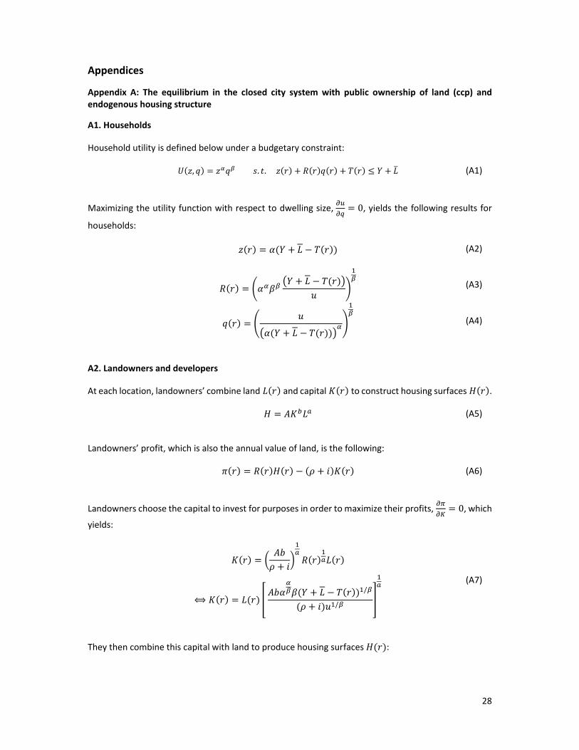
A1. Households

Household utility is defined below under a budgetary constraint:

𝑈 𝑧, 𝑞 𝑧 𝑞 𝑠. 𝑡. 𝑧 𝑟 𝑅 𝑟 𝑞 𝑟 𝑇 𝑟 𝑌 𝐿 (A1)

Maximizing the utility function with respect to dwelling size, 0, yields the following results for

households:

𝑧 𝑟 𝛼 𝑌 𝐿 𝑇 𝑟 (A2)

𝑅 𝑟 𝛼 𝛽𝑌 𝐿 𝑇 𝑟

𝑢 (A3)

𝑞 𝑟𝑢

𝛼 𝑌 𝐿 𝑇 𝑟 (A4)

A2. Landowners and developers

At each location, landowners’ combine land 𝐿 𝑟 and capital 𝐾 𝑟 to construct housing surfaces 𝐻 𝑟 .

𝐻 𝐴𝐾 𝐿 (A5)

Landowners’ profit, which is also the annual value of land, is the following:

𝜋 𝑟 𝑅 𝑟 𝐻 𝑟 𝜌 𝑖 𝐾 𝑟 (A6)

Landowners choose the capital to invest for purposes in order to maximize their profits, 0, which

yields:

𝐾 𝑟𝐴𝑏

𝜌 𝑖𝑅 𝑟 𝐿 𝑟

⟺ 𝐾 𝑟 𝐿 𝑟 𝐴𝑏𝛼 𝛽 𝑌 𝐿 𝑇 𝑟 /

𝜌 𝑖 𝑢 /

(A7)

They then combine this capital with land to produce housing surfaces 𝐻 𝑟 :

29

𝐻 𝑟 𝐴𝑏

𝜌 𝑖𝑅 𝑟 𝐿 𝑟

⟺ 𝐻 𝑟 𝐴 𝐿 𝑟 𝑏𝛼 𝛽 𝑌 𝐿 𝑇 𝑟 /

𝜌 𝑖 𝑢 /

(A8)

A3. Solving the urban system

Households numbers at each distance, 𝑟, can be expressed as the housing surface at each point divided by the size of each apartment. The available land at distance r is 𝐿 𝑟 𝑙𝑟, with 𝑙 2𝜋 in a perfectly circular city. We also assume linear transport costs which increase with the distance to the city center,

𝑇 𝑟 𝑝𝑟. Additionally setting 𝛾 0, 𝐵 𝐴 𝛼 , we get:

𝑛 𝑟𝐻 𝑟𝑞 𝑟

𝑏𝛽𝜌 𝑖

𝐴 𝛼 𝐿 𝑟𝑌 𝐿 𝑇 𝑟

𝑢

⟺ 𝑛 𝑟 𝐵 𝑙𝑟𝑌 𝐿 𝑇 𝑟

𝑢

(A9)

When the agricultural rent 𝑅 0, then the distance from the center to the city border is the location

where 𝜋 𝑟 0, which is:

𝑟 𝑌 𝐿 /𝑝 (A10)

We can now compute the utility of households by solving (A11):

𝑁 𝑛 𝑟 𝑑𝑟 (A11)

Which yields:

𝑢 𝑙𝐵𝑌 𝐿

𝛾 1 𝛾 𝑁𝑝 (A12)

The land rents recycled in the economy to households, 𝐿, are given by solving equation (A13):

𝐿1𝑁

𝜋 𝑟 𝑑𝑟 (A13)

Which gives:

30

𝐿1

𝛾 1𝑌 (A14)

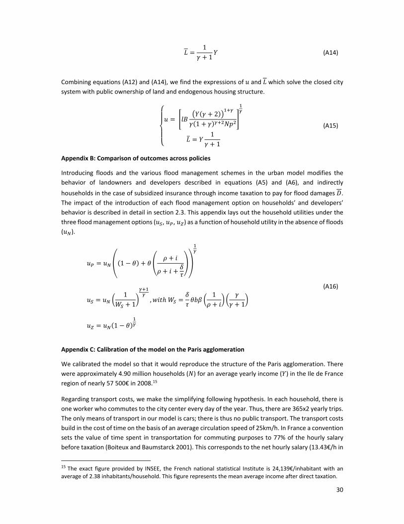
Combining equations (A12) and (A14), we find the expressions of 𝑢 and 𝐿 which solve the closed city system with public ownership of land and endogenous housing structure.

⎩⎪⎨

⎪⎧

𝑢 𝑙𝐵𝑌 𝛾 2


𝐿 𝑌1

𝛾 1

(A15)

Appendix B: Comparison of outcomes across policies

Introducing floods and the various flood management schemes in the urban model modifies the

behavior of landowners and developers described in equations (A5) and (A6), and indirectly

households in the case of subsidized insurance through income taxation to pay for flood damages 𝐷.

The impact of the introduction of each flood management option on households’ and developers’

behavior is described in detail in section 2.3. This appendix lays out the household utilities under the

three flood management options (𝑢 , 𝑢 , 𝑢 ) as a function of household utility in the absence of floods

(𝑢 ).

𝑢 𝑢 1 𝜃 𝜃𝜌 𝑖

𝜌 𝑖𝛿𝜏

𝑢 𝑢1

𝑊 1, 𝑤𝑖𝑡ℎ 𝑊

𝛿𝜏

𝜃𝑏𝛽1

𝜌 𝑖𝛾

𝛾 1

𝑢 𝑢 1 𝜃

(A16)

Appendix C: Calibration of the model on the Paris agglomeration

We calibrated the model so that it would reproduce the structure of the Paris agglomeration. There

were approximately 4.90 million households (𝑁) for an average yearly income (𝑌) in the Ile de France region of nearly 57 500€ in 2008.15

Regarding transport costs, we make the simplifying following hypothesis. In each household, there is

one worker who commutes to the city center every day of the year. Thus, there are 365x2 yearly trips.

The only means of transport in our model is cars; there is thus no public transport. The transport costs

build in the cost of time on the basis of an average circulation speed of 25km/h. In France a convention

sets the value of time spent in transportation for commuting purposes to 77% of the hourly salary

before taxation (Boiteux and Baumstarck 2001). This corresponds to the net hourly salary (13.43€/h in

15 The exact figure provided by INSEE, the French national statistical Institute is 24,139€/inhabitant with an average of 2.38 inhabitants/household. This figure represents the mean average income after direct taxation.

31

2008) assuming 23% of social charges. The Ile de France region being by far the richest region in France

we have considered that this unitary salary was increased by 25% in our runs.16 The other transport

costs encompass both the cost of fuel and the maintenance costs of the vehicle (insurance, garage

fees). They are established by relying on the reimbursement calculations by URSSAF (French tax

perception center) for usage of private vehicles for work purposes assuming an average mileage of

12000km/year.

The parameters that characterize both the utility function and the construction function are borrowed

from a detailed study conducted on the Paris agglomeration with the same albeit more precise

modeling framework, NEDUM (Viguié and Hallegatte 2012; Viguié, Hallegatte, and Rozenberg 2014;

Avner, Rentschler, and Hallegatte 2014). Parameter 𝛽 of the utility function represents the share of the net households’ budget17 devoted to housing expenses. It is estimated to be constant throughout

the agglomeration and equal to 30%. By construction, the parameter 𝛼, which is the share of the net budget allocated to expenses other than transport and housing is 70%. For the construction function,

the calibration done for the studies previously mentioned gives 𝐴 equal to 2.014, 𝑏 is 0.64 and 𝑎 is 0.36. These values enable the construction function to reproduce fairly accurately the costs/m² given

by the CSTB (“Centre socio‐technique du bâtiment” a French public‐private center devoted to the study

of buildings and building materials) as a function of the number of floors of a building.

Finally, buildings are supposed to be built for a century which gives us a depreciation rate 𝜌 of 0.01. The interest rate 𝑖 which provides the cost of capital is set at a value of 5%.

16 This figure is very close to the increase in the yearly income by inhabitant of the Ile de France compared to the average in France (INSEE). 17 The net budget of a household must be understood as the income minus transport costs.