Monte Carlo Simulation of Economic Capital Requirement …

19Monte Carlo Simulation of Economic Capital Requirementand Default Protection Premium

This paper presents a simulation framework for measuring and managing the default

risk of a loan portfolio. The economic capital requirement is explored for a hypothetical

credit portfolio through the dependency of counterparty default on a systematic risk

factor. The study employs bivariate standard normal distribution for mapping asset

return correlations into default correlations. Monte Carlo simulations are employed to

approximate the loss distribution and estimate various risk measures. The analysis

performed shows that the Asymptotic Single Risk Factor (ASRF) model is a fast way for

generating heavy-tailed credit loss distributions. Further, complete analytic derivation of

Basel II-IRB risk weight functions are reported. The paper also comments on the pricing

of single-period Portfolio Default Swaps.

Monte Carlo Simulat ion of Economic Capi tal Requi rementand Defaul t Protect ion Premium

Introduct i on

Credit risk is the dominant source of risk for commercial banks and is also the subject of extensive

research over the past few decades. It is typically defined as the risk of loss resulting from the failure of

borrowers to honor their payments. Recent advances in credit risk analytics have led to the proliferation

of a new breed of sophisticated portfolio risk models. These models play an increasingly important

role in banks’ risk management strategy. The calculation of potential losses and of the required capital

cushion is imperative in the competitive lending business since capital is one of the most expensive

resources. In contrast to VaR models for market risks, credit risk models focus in general on analysis of

the effects of credit rating transitions on changes in the value of a credit portfolio. The portfolio

approach incorporates concentration risk through the modeling of default correlations.

The idea that a bank’s capital should be related to the “riskiness” of its assets enjoys widespread

support. This idea underlies many banks’ internal decisions about capital and is central to the current

proposals for reform of the Basel Capital Accord. The June 2004 document of the Basel Committee on

Banking Supervision (BCBS)—International Convergence of Capital Measurement and Capital

Standards: A Revised Framework—follows a series of three consultative papers on the New Basel

Capital Accord (Basel II) stretching back to 1999. The Accord proposes two basic approaches for

Amit Kulkarni*

* Assistant Professor, National Institute of Bank Management, Pune, India. E-mail: [email protected]

© 2007 IUP. All Rights Reserved.

The IUP Journal of Bank Management, Vol. VI, No. 2, 200720

computing capital requirements for credit risk, viz, the Standardized Approach and the Internal Ratings-

Based (IRB) Approach (further divided into Foundation IRB and Advanced IRB). The capital requirement calculated on the basis of any of these two approaches is termed as Regulatory Capital. On the

contrary, Economic Capital is usually defined as the capital level that is required to cover the bank’sfuture losses at a given confidence level. Quite analogous to market risk VaR models, internal credit

risk models and Monte Carlo simulations are employed for estimating the economic capital requirement.It is generally assumed that it is the role of loan-loss reserves and provisions to cover Expected Losses,

whereas, bank capital should cover Unexpected Losses incurred over and above the expected losslevel. Thus, the required economic capital is the amount over and above the expected losses necessary

to achieve the Target Insolvency Rate (0.1% under IRB Approach)1. In Chart 1* (Appendix 3), for atarget insolvency rate equal to the shaded area, the required economic capital equals the distance

between the two lines. In practice, the target insolvency rate is usually chosen to be consistent with thebank’s desired credit rating. For example, if the desired credit rating is AA, the target insolvency rate

should equal the historical one-year average default rate observed for AA-rated firms. Economiccapital determination also forms the basis for computing the Risk-Adjusted Return On Capital (RAROC)

for the bank. A stated goal of the New Basel Accord is to keep the overall level of capital in the globalbanking system from changing significantly, assuming the same degree of risk; however, that does not

mean that the capital levels of each bank will remain unchanged (Saidenberg and Schuermann,2003). The Accord also attempts to end the Regulatory Capital Arbitrage, in which the most sophisticated

institutions shift exposures off their balance sheets to avoid an overly stringent regulatorycapital charge.

Against this backdrop, the present study may essentially be considered as a simulation exercise in

portfolio credit risk modeling. A key fact that is to be established at the outset is that the simulationframework presented in this paper can very well be generalized for internally-rated actual bank portfolio,

provided the bank has collected data on key borrower and facility characteristics. In the absence ofsuch bank proprietary data, an attempt is made to determine the economic capital required, over one-

year horizon, against a hypothetical credit portfolio with the following stylized features:

• The portfolio comprises 500 unsecured corporate exposures;

• Exposure at Default (EAD) per exposure is one rupee;

• Loss Given Default (LGD) per exposure is assumed equal2;

• The exposures are assigned CRISIL’s facility-wise long-term ratings (AAA, AA, A, BBB, BB, Band C);

• The distribution of 500 exposures across various rating grades is based on CRISIL’s one-yearaverage transition matrix for the period 1992-2005 (refer Tables 1, 2** and Chart 2); and

1 BCBS increased the confidence level in risk weight functions from 0.995 to 0.999 in November 2001.2 Under the IRB Foundation approach, senior unsecured claims on corporates are assigned 45% LGD and

subordinated unsecured claims are assigned 75% LGD. In the presence of collateral, LGD is adjusted downwardsbased on Collateral Adjustment formula. However, in this paper, Credit VaR has been computed based on threedifferent constant LGD rates (45%, 70% and 100%). The results of Bakshi et al. (2001) indicated that a modelwith a stochastic recovery rate performs equally well as a model with a constant recovery rate. Also note that the words ‘Obligors’, ‘Exposures’ and ‘Assets’ have been used interchangeably.

* All the charts are presented in Appendix 3; ** All the tables are presented in Appendix 4.


• Default-Mode paradigm is employed for scenario generation3 because absence of credit curvein India obstructs the MTM framework.

The study employs bivariate standard normal distribution4 for translating asset return correlationsinto default correlations. It offers a comparative anatomy of two especially influential returns simulationtechniques, viz, Asymptotic Single Risk Factor model (Vasicek, 1987) and J P Morgan’s RiskMetrics

algorithm to simulate correlated normal random variables based on Singular Value Decomposition(SVD). These simulations provide the vital structure for generating credit portfolio losses. Based onthe loss distributions, Credit Value at Risk (VaR) and economic capital requirement at 99.9% confidence

level is worked out. The results are subsequently evaluated against the capital required under IRBApproach of Basel II Accord. The paper also sheds some light on the issue of credit risk transfer. Itcomments on the cost of hedging the default risk of the simulated portfolio through the use of single-

period Portfolio Default Swaps (PDS). Assuming another restricted portfolio of 50 assets, the CapitalMultiplier (CM) implied under Internal Analytical Model at VaR

99.9% has been calibrated as well. In

Appendix 1, entire analytic derivation of IRB risk weight functions is produced. The key contribution

of this paper is that it provides a statistically rigorous and easily interpretable method for computingasset correlations between any two rated obligors, which in turn facilitates modeling of defaultcorrelations and simulation of portfolio losses. In addition, the method can straightforwardly compute

correlations for banks’ internally rated SME exposures and other non-traded firms, for which multifactorcorrelation approach (e.g., CreditMetrics and KMV) is impracticable.

Section 2 provides literature review, Section 3 sets out the modeling framework for generating loss

distribution and pricing of Portfolio Default Swaps, Section 4 reports the results and Section 5 concludes.

2. Literature Review

Over the past several years, as number of researchers have examined the modeling of Credit VaR and

pricing of credit derivatives. Several papers addressing these issues are available on the internet.

However, the received literature has mainly been located in the context of developed economies. See

for example, Jones and Mingo (1998), Koyluoglu and Hickman (1998), Nishiguchi et al., (1998),

Finger (1999), Ong (1999), Schönbucher (2000), Wilde (2001) and Xiao (2002) for calibration of

economic capital requirement. Similar studies undertaken within emerging economies are virtually

non-existent. BCBS, in its April 1999 publication, reported the results of the survey undertaken of the

current practises and issues in credit risk modeling. The survey was based on the modeling practices

at 20 large international banks located in ten countries. It identified data limitations and methodological

inconsistency as two major shortcomings of the current modeling practises. Also the survey results of

the US Federal Reserve Task Force can be referred on Internal Credit Risk Models (May 1998). In July

2005, BCBS released an explanatory note on the Basel II IRB risk weight functions. It focuses on

explaining the Basel II risk weight formulas in a non-technical way by describing the economic

foundations as well as the underlying mathematical model and its input parameters. Procyclicality of

3 Banks generally adopt either a Default-Mode (DM) paradigm or a Mark-to-Market (MTM) paradigm fordefining credit losses. Default-Mode is sometimes called a “binomial” model because only two outcomes arerelevant: non-default and default. It ignores the gains or losses arising due to rating changes. As against this,Mark-to-Market paradigm incorporates the impact of changes in the creditworthiness of borrowers, short ofdefault. J P Morgan’s CreditMetrics is based on MTM framework, whereas, Credit Suisse Financial Product’sCreditRisk+ is DM driven.

4 Bivariate Normal CDF add-in for MS Excel is freely downloadable on the internet.


economic capital is yet another issue that comes up a great deal in the discussions on IRB approach.

Lowe (2002) and Allen and Saunders (2003) offer an excellent literature review on the same. They

forcefully argue that a system of risk-based capital requirements is likely to deliver large changes in

minimum requirements over the business cycle, particularly if risk measurement is based on market

prices. Carlos and Céspedes (2002), d-Fine Consulting (2004), Jacobs (2004) and Cornford (2005)

explore the issues and challenges in implementing Basel II Accord. They expect the implementation to

be a large-scale exercise, making major demands on bank supervisors and requiring extensive technical

assistance, especially for developing countries.

Default correlations play a crucial role in virtually all fields of credit risk analysis. Many papers have

explored and grappled with the complexities of correlated defaults. For empirical evidence on modeling

of joint defaults and firms’ correlations, refer Li (2000), Dullmann and Scheule (2003), Servigny and

Renault (2003) and Hahnenstein (2004). Lopez (2002) assesses the validity of the assumption of

inverse relationship between asset correlation and default probability underlying the IRB capital rules.

Bangia, Diebold, and Schuermann (2000) and Fraser (2000) discuss the basic ideas in stress testing

credit portfolio models. Ranciere (2001) and Minton et al., (2005) assess the credit derivatives market

structure in emerging economies and US. For structuring and pricing of these products, refer

Schönbucher (2003), Bomfim (2005) and Elizalde (2005). O’Kane and McAdie (2001) and Houweling

and Vorst (2005) present empirical evidence on the pricing of credit default swaps. Their findings fully

document the occasional mispricing and arbitrage opportunities that arise in this market.

3. Modeling Framework

In this, the first section supplies the necessary theoretical context to exercise, the second sectionillustrates the simulation framework, and the third assesses estimation of single-period Portfolio DefaultSwap (PDS) Premium.

3.1. ‘Asymptotic Single Risk Factor’ Model

The modeling framework for simulating credit portfolio losses is presented below. While being

analytically tractable, it builds on the seminal work of Merton (1974) and Vasicek (1987). Vasicek

model leads to simple analytic asymptotic approximation of loss distribution and the VaR. The

approximation works very well when the portfolio is of large size and there is no exposure concentration,

i.e., the portfolio is not dominated by a few loans. In this model, the end-of-period borrower’s state

(Default or

No-default) is driven by an unobserved latent random variable Ri. In particular, for a hypothetical firm

i, default occurs if the firm’s asset return Ri falls below a given threshold C

i at a given time t. Although

Ri is unobservable, the firm’s asset value V

i may be derived through the application of Merton model

(Kulkarni et al., 2005, for Indian study). Hence, firm i defaults at time t if and only if,

titi R C ,, � � ... (1)

The returns have been normalized, thus,

i

ititi

RR

� V

� P� �� { ,

,

� �... (2)


where,R�� are “raw” non-standardized returns, whereas, i�P and i�V are the mean and standard

deviation of .iR��

)1,0(~, NR ti ... (3)

Note that, by working with standardized returns, all the firms in the portfolio have the standardnormal return distribution. The unconditional default probability for any firm is given by,

)()(Pr iiii CNCRW � �� ... (4)

where, (.)N is the cumulative standard normal distribution function.

The unconditional default probability, iW may very well be approximated on the basis of average

one-year default rate reported by agency rating transition matrix. Based on Wi, the return thresholds

iC can be extracted through equation 4,

)( ii WNC 1�� ... (5)

Asymptotic Single Risk Factor (ASRF) model assumes that the firm’s asset returns are function of

a single systematic factor, X and a firm-specific idiosyncratic factor, i�•

tiititi XR ,, 1 �H�E�E �� ... (6)

The systematic factor could represent the state of the economy. It affects all the firms in the portfolio

through the sensitivity coefficient �E. As �E increases, the returns are principally influenced by X; as

�E decreases, idiosyncratic risk prevails. In the limit, as �E tends to zero, the returns are completely

driven by the firm-specific risk factor i�• . To be consistent with the definition of Ri as a standard normal

random variable, X and i�• are standardized as well; they have zero mean and unit variance.

)1,0(~ NXt ... (7)

)1,0(~, Nti�• ... (8)

It is further assumed that Xtand ti,�• are uncorrelated and that they are serially independent;

hence,

0),(),(),( ,,, � �•�•� � �• �� stitistttit CovXXCovXCov ... (9)

It is easy to verify that equations 6 to 9 jointly establish equation 3. In light of equation 6, it can be

shown that �E plays a crucial role in capturing the degree of asset return correlation between any two

given firms. The unconditional correlation, i.e., the correlation coefficient independent of the valuetaken by the systematic factor X, and the unconditional covariance between returns R

i and R

j can be

expressed as:


jitjtitjti RRCovRRCorr � E� E� � ),(),( ,,,, ... (10)

Therefore, the degree of asset correlation is determined by the sensitivity of Ri to the systematic

factor X. In summary, a low correlation implies that the credit problems faced by borrowers are largelyindependent of each other; they are due to the idiosyncratic risk a particular borrower is exposed to.On the other hand, a higher asset correlation would suggest that credit difficulties occur simultaneouslyamong borrowers in response to a systematic risk factor, such as general economic conditions. Theconditional mean, variance and covariance of the asset returns, given any specific realization of X are,

titti XXRE � E� )|( , ... (11)

itti XR Var � E� �� 1)|( , ... (12)

0)|,( ,, � ttjti XRRCov ... (13)

Equation 13 implies:

0� )X|,R(RCorr ttj,ti, ... (14)

The conditional default probability for a firm may be written as:

�¸�¸

�¹

�·

�¨�¨

�©

�§

��

�� t

i

tiititiiti X

XCXCRXW

1Pr)|(Pr)( ,

� E

� E� H ... (15)

wherein, Xt is a realized value.

The unconditional probability of joint default between firms i and j is:

�� jijijjiiji CCNCRCRW � E� E,,ˆ)&(Pr, � � �� ... (16)

where, (.)N̂ is the cumulative distribution function of the bivariate standard normal distribution.

After developing this view, from Schonbucher (2000), now it can be written out the default correlation

between firms i and j as:

))(1)(())(1)((

)()(),,(ˆ,

jjii

jijijiji

CNCNCNCN

CNCNCCNP

� ��

� ��

� E� E... (17)

Thus, default correlation is a function of default thresholds iC and asset correlation i� E j� E.

The CreditMetrics methodology constructs estimates of the firms’ individual asset correlations from

market indices by means of a multifactor model. Within this approach, both country and industry

weights are assigned to each firm according to its Degree of Participation. For a portfolio comprising

n obligors, empirical estimates of n (n – 1) / 2 pairwise asset correlations are required. This produces

4950 asset correlation estimates for a meager 100-asset portfolio; however, almost all the commercial

banks hold credit portfolios reasonably larger than this. Moreover, the problem of using equity


correlations as a proxy for asset correlations has already been recognized as a potential drawback by

the model’s inventors themselves. It has recently been attacked on theoretical and empirical grounds

by Zeng and Zhang (2002) of KMV. Besides, Basel II doesn’t truly encourage full correlation modeling,

such as CreditMetrics and KMV multifactor models, and neither does it insist on banks to generate their

own internal estimates of asset correlations. This is essentially due to both the technical challenges

involved in reliably deriving and validating these estimates for specific asset classes and the desire for

consistency. Owing to these shortcomings, multifactor correlation modeling seems ill suited for the

present study. Moreover, the study being purely a simulation exercise, and not based on actual credit

portfolio data and equity prices, multifactor approach is infeasible as well. Therefore, the Basel II IRB,

June 2004 formula itself is employed for estimating asset correlation based on average (unconditional)

default probability of various rating grades. This formula is grounded primarily on the empirical

studies undertaken by the Basel Committee. The credibility of this approach has a critical bearing on

two assumptions: first, all firms within the same rating class have the same default rate, and hence, the

same asset correlation (R); and second, that the asset correlation is inversely related to probability of

default (PD). Intuitively, this can be explained as: the higher the PD, the higher the idiosyncratic risk

component of a borrower. And so, the default risk depends less on the overall state of the economy

and more on individual risk drivers.

�¸�¸�¹

�·�¨�¨�©

�§

��

��¸

�¸�¹

�·�¨�¨�©

�§

��

��

��

��

��

��

50

*50

50

*50

1

1124.0

1

112.0

e

e

e

eR

PDPD

... (18)

Basel II risk weight functions implicitly assume an infinitely-granular homogeneos portfolio,

wherein, all the obligors falling within a given risk-class have similar PD. Thus, from equation 18,

all such obligors are assigned similar correlation coefficient. R is an input in the IRB risk weight

function, which itself has its origin in Vasicek’s homogeneous portfolio framework. Consequently, “R

may be interpreted as the asset correlation between any two firms falling in the same rating-bucket”. As

an illustration, let the given risk bucket comprise N homogenous obligors. All such obligors hold

similar credit rating and PD. From equation 10, the asset correlation between obligor N1 and any

other obligor )1( �ziNi may be written as:

)1(1)1(,1 �z�z � iNiNiNiNCorr �E�E ... (19)

Since the obligors belong to the same risk category, from equation 18, they have equal asset

correlation coefficient,

RRR iNiN � � �? �z )1(1 ... (20)

Being homogeneos, they possess similar sensitivity )( �E to the systematic risk factor X.

�E�E�E � � �? �z )1(1 iNiN ... (21)


From equations 19, 20 and 21,

RCorr iNiN � � � � z � E� E� E)1(,1 ... (22)

R� � ? � E ... (23)

On similar lines, the asset correlation between any two firms i and j representing two differentrating grades, say A and B respectively, may be expressed as a product of their sensitivity coefficients,

BjAiBjAiCorr � E� E� , ... (24)

where, AiAi R� � E ... (25)

and BjBj R� � E ... (26)

In this paper, as 500 assets have been allocated over seven different rating grades, there would be28 distinctive ratings-based asset correlation estimates between any two exposures in the portfolio;this is inclusive of the seven estimates for exposures with similar ratings (refer diagonal elements of

Table 4). These correlations provide the foundation for simulating portfolio losses.

3.2 Determination of Economic Capital Requirement

Basel II document provides the risk weight functions for calibrating the capital requirement under IRBapproach. The output is dependent on the estimates of PD, LGD, EAD, asset correlations, effectivematurity and sales turnover (refer Appendix 1). The resulting capital requirement is termed as RegulatoryCapital. On the contrary, determination of Economic Capital necessitates developing an internalmodel for simulating credit portfolio losses. In this paper, the two distinct simulationtechniques that are taken are the ASRF model (equation 6) and RiskMetrics 1996 algorithmto simulate correlated normal random variables based on Singular Value Decomposition (SVD) of asset returns covariance matrix.

3.2.1 Simulat ions Based on ASRF Model

Asset return simulation, being a prerequisite for generating portfolio loss distribution, is performed

through the following steps:

Step 1: Assign values to the key model parameters, iC i and � E. For instance, equation 25 gives

value of i� E for each rating grade, whereas, equation 5 gives .iC

Step 2: For each scenario, generate 501 standard normal random values representing one draw

for the systematic factor X and 500 draws for the idiosyncratic factor i� • per exposure.

This translates into total 32.8155 million random draws for the 500 assets portfolio over

65,500 scenarios.

Step 3: Through equation 6, compute asset return, iR for each exposure (per scenario) and compare

it against threshold, iC to record the occurrence of default.


Step 4: Once total defaults have been counted and recorded over each scenario generated, the

portfolio Expected Loss ( PEL ) and frequency distribution for the Total Defaults per Scenario

(0 to 500) is computed. This necessitates construction of “bins” per default loss-size. Actual

loss distributions are estimated assuming three different constant LGD rates, i.e., 100%, 70%

and 45%.

Step 5: Based on the frequency distribution of simulated losses, VaR at 99.9% confidence level is

worked out. This figure goes into the estimation of Economic Capital.

PELVaREC �� %9.99 ... (27)

The output from the above equation is subsequently evaluated against the capital required underIRB Approach of Basel II Accord.

Expected Shortfall (ES)

In the literature on risk management, VaR has shown itself to be a very useful risk measure. However,it is also now widely accepted that VaR is not the finest risk measure available (Acerbi and Tasche,2002; Rockafellar and Uryasev, 2002). VaR is often criticized for its failure to reflect the severity of

losses in the worst scenarios in which the loss exceeds VaR. In other words, VaR is not a measure of theheaviness of the tail of the distribution. A novel theoretical development in recent years is the ExpectedShortfall (ES), a measure that is sometimes also known as Conditional VaR or Tail VaR. ES is the

expected value of the losses, L, if loss is in excess of VaR. The VaR tells the most what can be expectedto lose if a bad (i.e., tail) event does not occur. However, in direct opposition to this view, ES tells whatcan be expected to lose if a tail event does occur. It reflects the losses incurred in the tail region (beyond

VaR) of the loss distribution. ES is preferable to VaR because it satisfies the highly desirable propertiesof coherence, which the VaR, in general, does not. The presence of heavy tailed loss distributionsignificantly elevates the ratio of ES to VaR. Thus, ES being more conservative a risk measure than

VaR, it is expected to be written as:

]|[)( �D�D VaRLLELES �t� ... (28)

3.2.2 Simulations Based on RiskMetrics SVD Algorithm

RiskMetrics Document, in its Appendix E, introduced three algorithms for simulating correlated normal

random variables from a specified covariance matrix ;�6 it is square and symmetric. The algorithmswere Cholesky Decomposition (CD), Eigenvalue Decomposition (ED) and the Singular ValueDecomposition (SVD). CD is efficient when�6 is positive definite. However, CD is not applicable for

positive semi-definite matrices. ED and SVD, while computationally more intensive, are usefulwhen �6 is positive semi-definite. The decomposition is necessary in order to reproduce the originalmatrix �6 from the simulated returns; the reproduced covariance matrix*�6 should closely match

original matrix�6. Further discussion on this subject is available in Ong (1999) and d Fine (2004). Inthe present study, SVD for simulating correlated asset returns is employed5. “However, for the sake ofbrevity, the base portfolio size has been restricted only to 10% of the original portfolio, i.e., total 50

exposures allocated across the seven rating grades (refer Table 14)”. Economic Capital estimatedthrough SVD algorithm is further compared against similar estimate obtained under ASRF model

5 Results on matrix decomposition are available on request from the author.


simulation framework of Section (3.2.1) for the restricted portfolio. The Capital Multiplier (CM) impliedunder Internal Analytical Model at %9.99Var is calibrated as well for this 50-asset portfolio (referAppendix 2).

3.3 Estimation of Single-period PDS Premium

Credit derivatives permit the transfer of credit risk without the need to liquidate positions in theunderlying instruments. Internationally, the rapidly expanding credit derivatives market has created alarge set of instruments for credit risk management. An increasingly popular product is the CreditDefault Swap (CDS), wherein, one party purchases credit protection from another to cover the creditloss of an asset following a credit event. The credit default premium is paid at periodic intervalsthroughout the swap tenor. Since banks hold very large loan portfolios, they would find it rathereconomical to buy protection through a single Portfolio Default Swap (PDS) as against multiple CDS.The reason for this belief is essentially the default correlation structure embedded in the credit portfolio;the correlation structure provides diversification benefits to the counterparties. PDS offers protectionfor a given fraction (loss tranche) of the total portfolio value. The credit losses incurred beyond thetranche are borne by the bank itself6.

Estimation of protection premium entails modeling various credit risk parameters, such as,PD, LGD and default correlation. The hazard rate approach, based on the seminal work of Jarrow andTurnbull (1995), has gained prominence in credit derivatives literature. This approach employs marketdata on credit spreads or CDS spreads for calibrating Protection Premium. However, the absenceof CDS market, coupled with illiquid corporate bond market in India (Sharma and Sinha, 2005)preempts the possibility of employing hazard rate approach in this study. Therefore, the premium hasto be derived through the simulated loss distribution of protected tranche. This distribution is flat at thetranche-boundaries owing to the possibility of portfolio loss exceeding the loss tranche, and thisfeature becomes more pronounced when the tranche is narrowed. Ours is only a one-period approachand it assumes that defaults occur only at the year-end (this simplifies the treatment of accrued premium).It ignores the survival probability of individual credits beyond one year. In other words, the PDSdoesn’t offer default protection beyond one-year. Counterparty credit risk is further assumed among,or that, it gets managed through collateral requirement. For the 500 assets portfolio, First-Loss ProtectionPremium is reported over eight different First-Loss Tranches. However, Second-Loss Tranche is prefixed

to the size of 20 defaults, observed beyond each of the First-Loss Tranches (refer Tables 19 and 20).

The methodology employed for pricing the single-period PDS is eloborated as:

Step1: Simulate the ASRF model-based loss distribution (100% LGD) for the 500 assets portfolio;

Step2: Subject to the size of First-Loss Tranche, allocate the losses to the First-Loss Protection Seller–

Example: The size of First-Loss Tranche is 30 defaults. For each default-bin from 1 to 30,allocate the entire value of actual defaults observed and losses incurred to the First-LossProtection Seller. However, when defaults exceed 30 credits, the First-Loss Protection Seller isto bear losses only to the extent of 30; the excess being borne by the Protection Buyer himselfor by the Second-Loss Protection Seller (if any);

6 In case, the protection is bought only against any first default in the portfolio, the default swap is termed as‘First-to-Default’ Swap. On similar lines, one can structure ‘Second-to-Default’, ‘Third-to-Default’ or any‘Nth-to-Default’ Swap. Also note that RBI had issued draft guidelines on introduction of credit derivatives inIndia in March 2003.


Step 3: Generate loss distribution for the First-Loss Tranche;

Step 4: Compute expected value of the losses to be incurred by the First-Loss Protection Seller–

�¦ �¦� �¸�¸

�¹

�·

�¨�¨

�©

�§ �u�

N

i

iiFirstLoss

f

LfEL

1... (29)

where, iL depicts the losses allocated to the First-Loss Tranche (from Step 3), whereas, if represents

the frequency statistic for iL ;

Step 5: The Protection Premium payable upfront to the Protection Seller is computed as a percentage

of the size of First-Loss Tranche–

100,

Pr �u��

�u�

TrancheLosstSizeofFirsDEL

emium FirstLoss... (30)

where, D is the discount factor7 acceptable to both the counterparties; and

Step 6: Analogous to this, estimation of Second-Loss Protection Premium entails repeating the steps2 to 5.

4. Results

Table 1 presents Crisil’s one-year Average Rating Transition Matrix over the period 1992-2005. This

matrix is based on facility-wise long-term ratings of corporate bonds/debentures8. Crisil doesn’t factor

in the security provided (if any) or expected recovery in its bond ratings. The last column of the matrixreports the average default rate observed for various rating grades. One important fact to be pointedout is that historical default rate is virtually zero for AAA and AA ratings. However, Basel II Accord

prescribes a minimum default rate of 0.03% for obligors with the best credit quality. Therefore isemployed the floor rate of 0.03% for AAA and AA exposures. Also note that the default rate for B ratingmarginally exceeds that for C. Although this seems counter-intuitive, this evidence is taken into account

in the analytical framework. From Table 2 and Chart 2, it is evident that the distribution of exposuresacross various rating grades is skewed towards the investment-grade ratings of AAA, AA, A and BBB.This fact need not truly reflect the actual rating-wise exposure distribution observed at various commercialbanks. However, notwithstanding this limitation, the 500 assets portfolio is allocated based on Crisil’srating distribution because any study on rating-wise distribution of exposures at Indian banks isnon-existent. Also refer Table 3 for the unconditional (average) default probability and return thresholdscomputed for various rating grades.

The interrelationship between asset correlation and default correlation being a key objective of thisstudy, Tables 4 to 7 and Chart 3 elaborate on this linkage. In Table 4, the asset correlation between anytwo rated exposures is reported; the correlation coefficient is inversely related to the exposure’s PD(refer equation 18 of Section 3). The diagonal elements, in particular, emphasize this fact. Based onbivariate standard normal distribution, Table 5 reports the estimates for Joint Default Probability (JDP)

7 For the purpose of computational ease, the discount rate of 10% was employed in the study.8 In the absence of data on Obligor Ratings in India, Facility-wise Ratings was the only alternative available for

proceeding with the present study.


between the exposures. The figures are relatively high for the exposures rated at lower grades; the JDPseems positively related to the exposures’ individual PD levels. On similar lines, from Table 6, default

correlation between any two exposures is an increasing function of the individual PD estimates.A related implication is that for any two exposures which are rated alike (diagonal elements), asset

correlation and default correlation are inversely related (refer Chart 3). If the results are to be taken atface value, they suggest that at lower ratings and higher individual PD levels, asset correlation is low,

whereas, default correlation is high. This anomaly may be scrutinized through the following illustration–Example: Table 7 reports the default correlation between two firms with identical ratings; both are

either AAA or BBB. The lower PD for AAA firms translates into higher asset correlation coefficientunder IRB approach. On the contrary, for BBB firms, the value is relatively low. From equation 16 of

Section 3, JDP is jointly determined by asset correlation coefficient and individual PD levels. Lowerasset correlation for BBB rated firms should theoretically produce lower JDP and lower default correlation

coefficient vis-à-vis AAA rated firms. However, this effect is nullified and largely reversed by thehistorical default rate of BBB firms, which is quite high. Consequently, JDP and default correlation

estimate for BBB firms is higher than that for AAA firms, although the asset correlation is quite low forthe former.

Furthermore, the correlation between default probabilities is always less than the correlation

between asset values. The IRB risk weight functions employ estimates of asset correlation, and notdefault correlation, for calibrating capital requirement. Hence, “low rated exposures which carry smaller

asset correlation parameter, require higher allocation of bank capital owing to their PD and not dueto their higher implied default correlation parameter”. This vital conclusion is the terminus of the

above analysis.

Tables 8 to 11 and Chart 4 summarize the results of the ASRF model-based simulation exercise

performed for the 500 assets portfolio. Credit VaR, Expected Shortfall (ES) and Economic Capital (EC)requirement at 99.9% confidence level are reported at different LGD rates, i.e., 100%, 70% and 45%.

Assuming 70% constant LGD rate which was incidentally proposed in S & P Asia-Pacific Banking

Outlook 2004 for Indian credit assets, EC requirement works out to 8.516% of total exposure. It

declines still further to 5.48%, assuming 45% LGD. However, in case the bank intends to attain AArating at 99.97% confidence level (0.03% default rate from Table 3), it has to maintain capital at

11.363% (70% LGD). To carry the same argument further, presence of extreme events/fat tail in theloss distribution manifests itself in the form of significant ES to VaR ratio (refer Charts 5 to 7). In the

study, this ratio almost equals 1.54 as reported in Table 13. The reason for this can be traced to thesimulation trials having generated scenarios with default sizes as high as 466, 468, 477, 480 and 486

in the 500 assets portfolio. The skewness parameter of 7.022 and kurtosis of 235.46 further underlinethe presence of fat tail (refer Table 8). Assuming Beta distribution for the percentage credit losses, the

calibrated parameters �Dand �E are reported in Table 10. From Table 9, the capital requirement atVaR

99.9% (70% LGD) works out to Rs. 42.5845. As against this, the IRB risk weight functions produce

capital requirement @ 9% of RWA, of Rs. 47.2174 at the same LGD level (refer Table 12). Thus, thesimulation exercise does produce sizeable capital savings as against IRB approach. The results need

not significantly differ in case the credit portfolio is tilted towards the speculative-grade ratings of BB,

9 The IRB risk weight function is positively sloped, although relatively flat, for very low quality credits.


B and C9. In conclusion, note that the 95% confidence interval around Expected Loss (EL) undoubtedly

underlines the accuracy of the estimation results10. At 70% LGD, the EL of Rs. 9.9155 lies within a

narrow band of Rs. 9.8562 and Rs. 9.9747. This result therefore inspires confidence in the estimates.

The estimates are evidently free of the noise stemming from Monte Carlo simulations.

ASRF model and J P Morgan’s RiskMetrics SVD algorithm are the two prominent return-simulation

techniques available for generating credit loss distribution. A priori, the variation between VaR99.9%

estimates produced under these two approaches need not be substantial. Likewise, the capital

requirements should be near identical. The results addressing this issue are produced in Tables 14

and 15, restricting the size of base portfolio to 50 assets and LGD to 100%. As is evident from the

results, VaR and subsequent capital requirements are not truly equivalent under the two methods.

However, the difference between EL calibrated under these two techniques is statistically insignificant

at 95% confidence level. Whereas, the ASRF model generates Expected Shortfall of Rs. 11.08, the

estimate is Rs. 10.05 under SVD algorithm. On this ground, the ratio of ES to VaR equals 1.144 for

ASRF and 1.077 under SVD technique. Again, this divergence between the results largely emanates

from the fat tail produced through ASRF model based simulations. For the 50-asset portfolio, this

technique is relatively successful in producing default scenarios as large as 44, 47, 49 and 50. The

SVD algorithm, however, falls short of generating any default size larger than 21 and 25. Chart 11, in

particular, portrays the tails of these simulated loss distributions. The upshot of this analysis is that the

risk measures produced under ASRF model score high on the ground of conservatism. Moreover,

given the massive size of credit portfolios which banks actually hold and also the constraints on

computing power, ASRF model should be the preferred simulation technique. Besides, decomposition

of covariance matrix under SVD could turn out to be highly unwieldy for large portfolios. Even so,

inability to generate heavy tailed distribution is perhaps the supreme disadvantage of SVD method.

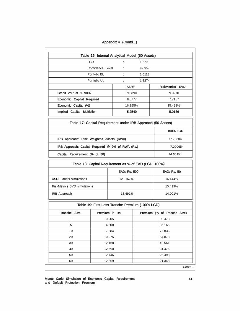
For the 50-asset portfolio, Capital Multiplier (CM) implied under Internal Analytical Model at

VaR99.9%

is reported in Table 16. It equals 5.2540 for ASRF model-based VaR, whereas, 5.0186 for

RiskMetrics SVD algorithm-based VaR. Also note that the capital requirement under Internal Analytical

Model is almost equal to the respective estimates from simulation techniques (refer Chart 8). Hence,

Monte Carlo simulations seem to reasonably duplicate the Internal Analytical Model results. In the

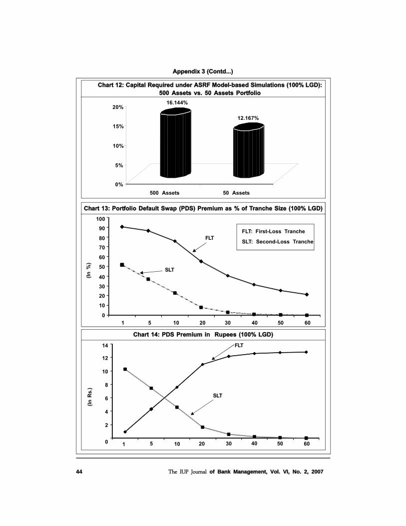
final analysis, Table 18 and Chart 12 shed some light on the benefits of diversification effect embedded

in much larger credit portfolios. This fact gets reflected in the ratio of economic capital to total exposure,

which is 16.144% for 50-asset portfolio and barely 12.167% for 500 assets portfolio. However, for the

50-asset portfolio, capital requirement of 14.001% calibrated under IRB Approach is far less than that

under simulation techniques and Internal Analytical Model (refer Chart 8). But the finding gets reversed

for the 500 assets portfolio (refer Chart 4).

In the conventional analysis, credit derivative premium is modeled through loss distribution based

on default probabilities and recovery rate of the reference asset/portfolio. An alternative approach,

commonly referred to as reduced-form, is to rely on the market data on credit spreads of traded

corporate bonds. However, the pursuit of this line of research gets seriously circumscribed in our study

on account of the fact that Indian private debt market is largely illiquid beyond investment-grade10 CreditMetrics Document, in Appendix B, proposes a methodology to construct confidence intervals around the

mean value of simulated portfolio losses. Thus, after generating N scenarios, it may be said 95% confidentlythat the true mean value of portfolio losses lies between m - 1.96 (s/Ö N) and m + 1.96 (s/Ö N). s/Ö N is thestandard error; the bands will tighten as N increases.


credits. Therefore it is relied on the former approach of modeling loss distributions for the protectionseller over one-year horizon. The results on measurement of single-period Portfolio Default Swap

premium [First-Loss Tranche (FLT) and Second-Loss Tranche (SLT)], receivable upfront by theprotection seller, on the 500 assets portfolio (100% LGD) are reported in Tables 19 and 20. In theanalysis, First-Loss Tranche was progressively increased as a given percentage of total portfolio, butthe Second-Loss Tranche was preset at 20 defaults observed beyond each of the First-Loss Tranches.As is evident from Chart 13, the percentage of First-Loss protection premium declines rapidly withgradual increase in tranche size. Similar are the dynamics for percentage of Second-Loss premium.However, it is interesting to note that the premium value, when denominated in rupees, increases forFirst-Loss Tranche and declines for Second-Loss Tranche at distant levels (refer Chart 14). A promisingcandidate for explaining this result is the shape of the loss distribution, which is positively skewed.Consequently, the probability of observing extreme losses beyond EL level are negligible but non-zero. And so, the premium charged for relatively larger First-Loss tranches increases in amount, butdeclines in proportion. Second-Loss premium however declines on both the counts, because atfarther levels, the Second-Loss protection tranche could hardly get invoked. Also refer Charts 15 to 17for the loss distribution of First-Loss Tranche and Second-Loss Tranche over the given tranche size.

Conclusion

Portfolio credit risk modeling is the tool for estimating required capital reserves against loan portfolio.In this study, Monte Carlo simulation approach was presented for analyzing and measuring credit riskin a number of ways. Given a hypothetical credit portfolio of 500 assets, assuming different LGD rates,ASRF model-based loss distributions were generated. Based on this, Credit VaR and EconomicCapital requirement at 99.9% confidence level was worked out. The estimate is 8.516% of totalexposure at 70% LGD. The simulation trials generated scenarios with default sizes as high as 466,468, 477, 480 and 486 in the 500 assets portfolio. Consequently, the ratio of Expected Shortfall toVaR turned out to be quite high, at around 1.54. Keeping in view that credit loss distributions are quiteoften heavy-tailed, coupled with the fact that the tail region is most relevant for risk management, theresults provide an interesting insight into the ongoing debate on the suitability of VaR as a riskmeasure. Be that as it may, the simulation exercise did succeed in producing sizeable capital savings asagainst IRB approach. For various rating grades, the study also mapped asset correlations into defaultcorrelations through bivariate standard normal distribution. The analysis concluded that the defaultcorrelation is positively related with the firms’ PD. However, the function is inverse for asset correlationand PD. Furthermore, the correlation between default probabilities is always less than the correlationbetween asset values.

A comparative anatomy of two distinct returns simulation techniques; ASRF model and J P MorganRiskMetrics algorithm to simulate correlated normal random variables through SingularValue Decomposition (SVD). The assessment was done for a restricted portfolio of 50 exposures. Theresults suggested that the risk measures produced under ASRF model simulations are relativelyconservative. Moreover, given the massive size of credit portfolios which banks actually hold and alsothe constraints on computing power, ASRF model should be the preferred simulation technique.Besides, matrix decomposition under SVD could turn out to be highly unwieldy for large portfolios.Even so, inability to generate heavy tailed distribution is perhaps the supreme disadvantage ofSVD method. For the 50-asset portfolio, Capital Multiplier (CM) implied under Internal Analytical


Model at VaR99.9%

is around 5.25. Also, Monte Carlo simulations seem to reasonably duplicate the

Internal Analytical Model results.

The evaluation of the issue of credit risk transfer estimated default protection premium for the 500

assets portfolio through the use of single-period Portfolio Default Swaps over two loss tranches, viz.,

First-Loss and Second-Loss Tranches. The percentage of First-Loss protection premium declined

rapidly with gradual increase in tranche size. Similar results were observed for percentage of Second-

Loss premium. However, given the premium value in rupees, the cost increased for First-Loss Tranche

and declined for Second-Loss Tranche at distant levels. This result has been attributed to the shape of

the loss distribution, which is positively skewed.

The analytics discussed elucidate the mechanics of calibrating Economic Capital within a simulation

framework. Since any study on portfolio credit risk undertaken within developing economies is virtually

non-existent, the present study could serve as a modest attempt to fill this gap. It is hoped that this

paper will kindle research interest in a number of other related issues, such as, stress testing credit

portfolio models and estimation of multi-period default protection premium.

References

1. Acerbi C and Tasche D (2002), “On the Coherence of Expected Shortfall”, Journal of Banking

and Finance, Vol. 26, pp. 1487-1503.

2. Allen Linda and Saunders Anthony (2003), “A Survey of Cyclical Effects in Credit Risk

Measurement Models”, BIS Working Paper No. 126.

3. Bakshi G, Madan D and Zhang F (2001), “Understanding the Role of Recovery in Default Risk

Models: Empirical Comparisons and Implied Recovery Rates”, Working Paper, University of

Maryland.

4. Bangia A, Diebold F, Kronimus A, Schagen C and Schuermann T (2000), “Ratings Migration and

the Business Cycle, with Application to Credit Portfolio Stress Testing”, Journal of Banking and

Finance, Vol. 26, pp. 445-474.

5. Basel Committee on Bank Supervision (1999), “Credit Risk Modelling: Current Practices and

Applications”, Working Paper (April).

6. Basel Committee on Banking Supervision (2004), “International Convergence of Capital

Measurement and Capital Standards: A Revised Framework”, (June).

7. Bomfim Antulio (2005), Understanding Credit Derivatives and Related Instruments, Elsevier

Academic Press.

8. Carlos Juan and Céspedes García (2002), “Credit Risk Modeling and Basel II”, Algo Research

Quarterly, Spring, Vol. 5, No. 1.

9. Cornford Andrew (2005), “Basel II: The Revised Framework of June 2004”, UNCTAD Discussion

Paper, No. 178.

Reference # 10J-2007-05-02-01

�+


10. d-Fine Consulting (2004), “The Basel II IRB Approach and Internal Credit Risk Models”,http://www.dfine.de/deutsch/Bibliothek/Forschungsarbeiten/DiplomaThesis%20LGD.pdf

11. Dullmann Klaus and Scheule Harald (2003), “Determinants of the Asset Correlations of GermanCorporations and Implications for Regulatory Capital”, http://www.bis.org/bcbs/events/wkshop0303/p02duelsche.pdf

12. Elizalde A (2005), “Credit Risk Models IV: Understanding and Pricing CDOs”,www.abelelizalde.com.

13. Finger Christopher C (1999), “Conditional Approaches for CreditMetrics Portfolio Distributions”,CreditMetrics Monitor, pp. 14-33.

14. Fraser Rob (2000), “Stress Testing Credit Risk Using CreditManager 2.5”, RiskMetrics Journal,

Vol. 1 (May).

15. Frye Jon (2001), “Weighting for Risk”, Working Paper, FRB Chicago (April) (S&R-2001-1)

16. Gersbach H and Lipponer A (2000), “The Correlation Effect”, Working Paper, University ofHeidelberg.

17. Gordy Michael (2002), “A Risk-Factor Model Foundation for Ratings-Based Bank Capital Rules”,Finance and Economics Discussion Series 2002-55, Board of Governors of the Federal ReserveSystem, Journal of Financial Intermediation.

18. Hahnenstein Lutz (2004), “Calibrating the CreditMetrics Correlation Concept for Non-PubliclyTraded Corporations: Empirical Evidence from Germany”, http://www.gloriamundi.org/picsresources/lhccm.pdf

19. Houweling Patrick and Vorst Ton (2005), “Pricing Default Swaps: Empirical Evidence”, Journal

of International Money and Finance, Vol. 24, pp. 1200-1225.

20. Jacobs Thomas (2004), “Risk Models and Basel II: A Review of the Literature”, http://www.business.uiuc.edu/c-kahn/Fin427/ThomasJacobs_Review.pdf

21. Jarrow R and Turnbull S (1995), “Pricing Derivatives on Financial Securities Subject to CreditRisk”, Journal of Finance, Vol. 50, No. 1, pp. 53-85.

22. Jones David and Mingo John (1998), “ Industry Practices in Credit Risk Modeling and InternalCapital Allocations: Implications for a Models-Based Regulatory Capital Standard”, FRBNY

Economic Policy Review (October).

23. Koyluoglu H Ugur and Hickman Andrew (1998), “Reconcilable Differences”, Risk Magazine(October), pp. 56-62.

24. Kulkarni Amit, Mishra Alok and Thakker Jigisha (2005), “How Good is Merton Model at AssessingCredit Risk? Evidence from India”, www.defaultrisk.com

25. Li David (2000), “On Default Correlation: A Copula Function Approach” , Journal of FixedIncome, Vol. 9, No. 4, pp. 43-54.

26. Lopez Jose (2002), “The Empirical Relationship between Average Asset Correlation, FirmProbability of Default and Asset Size”, Federal Reserve Bank of San Francisco Working Paper,Vol. 23 (April).


27. Lowe Philip (2002), “ Credit Risk Measurement and Procyclicality”, BIS Working Paper, No. 116.

28. Merton R C (1974), “On the Pricing of Corporate Debt: The Risk Structure of Interest Rates”,

Journal of Finance, Vol. 29, pp. 449-470.

29. Minton Bernadette A, Stulz René and Williamson Rohan (2005), “How Much Do Banks UseCredit Derivatives To Reduce Risk?”, NBER Working Paper, No. W11579.

30. Morgan J P (1996), RiskMetrics-Technical Document, Reuters, New York, USA.

31. Morgan J P (1997), CreditMetrics-Technical Document, New York, USA.

32. Nishiguchi K, Kawai H and Sazaki T (1998), “Capital Allocation and Bank Management Basedon the Quantification of Credit Risk”, FRBNY Economic Policy Review (October).

33. O’ Kane D and McAdie R (2001), “Explaining the Basis: Cash Versus Default Swaps”, FixedIncome Research, Lehman Brothers, London.

34. Ong Michael (1999), Internal Credit Risk Models—Capital Allocation and PerformanceMeasurement, Published by Risk Books.

35. Ranciere Romain (2001), “Credit Derivatives in Emerging Markets”, IMF Policy DiscussionPaper (April).

36. Rockafellar R T and Uryasev S (2002), “Conditional Value-At-Risk for General Distributions”,Journal of Banking and Finance, Vol. 26, No. 7 (July), pp. 1443-1471.

37. Saidenberg Marc and Schuermann Til (2003), “The New Basel Capital Accord and Questions

for Research”, FRBNY October 2003, Working Paper.

38. Schönbucher P (2000), “Factor Models for Portfolio Credit Risk”, Working Paper, University of

Bonn.

39. Schönbucher P (2003), “Credit Derivatives Pricing Models”, Wiley Finance.

40. Servigny A D and Renault O (2002), “Default Correlation: Empirical Evidence”, Working Paper,

Standard and Poor.

41. Sharma V and Sinha C (2006), “The Corporate Debt Market in India”, http://www.bis.org/publ/

bppdf/bispap26m.pdf

42. US Federal Reserve Task Force on Internal Credit Risk Models (1998), “Credit Risk Models atMajor US Banking Institutions: Current State of the Art and Implications for Assessments of

Capital Adequacy”, Committee Report (May).

43. Vasicek Oldrich (1987), “Probability of Loss on Loan Portfolio”, Working Paper, KMV Corporation

44. Wilde T (2001), “IRB Approach Explained”, Risk Magazine, Vol. 14, No. 5, pp. 87-90.

45. Xiao Jerry (2002), “Economic Capital Allocation for Credit Risk”, RiskMetrics Journal, Winter,Vol. 2, No. 2.

46. Zeng B and Zhang J (2002), “Measuring Credit Correlations: Equity Correlations are notEnough!”, Working Paper, KMV Corporation.


Appendix 1

Derivation of Basel II IRB Risk Weight Function

The ASRF model, coupled with Homogenous Portfolioassumption, forms the basis for IRB risk weightfunctions. The model assumes that for all the assets in the credit portfolio,

%100&,, � � � iii LGDCC� E� E

Secondly, the model assumes that all the assets in the portfolio are equally weighted. This guaranteesthat in a portfolio with N assets, the probability of observing k defaults is equivalent to the probabilityof observing k/N percentage of default losses.

Under Default Mode paradigm, the number of defaults (k) in the portfolio follow binomial distributionfor a given value of systematic risk factor X. Thus, if L is let to denote the fraction of defaults(percentage of default losses), then may be the conditional probability of observing a given losslevel written as,

kNk XWXWkNk

NX

Nk

L � ��

� ¸̧̧� ¹

� ·¨̈̈

� ©

� §� )](1[)(

)!(!!

Pr ... (A.1.1)

where, W(X) is the conditional default probability, as defined in equation 15 of Section 3

The major thrust of Large-Portfolio Approximation framework (Vasicek, 1987) is that for an infinitelylarge homogeneous portfolio, through the Law of Large Numbers,

)( XWXNk

LE � |¸̧̧� ¹

� ·¨̈̈

� ©

� §� � {� T ... (A.1.2)

where, �Tand L are the expected and actual values of percentage default losses in the portfolio,respectively. Equation A.1.2 may be construed as under:

Expected value of the fraction of obligors defaulting in the large homogenous portfolio ( �T), overa given time horizon, can be approximated by the corresponding individual conditional defaultprobabilities, denoted as W(X) of the obligors.

Note that for any given value of �T, one can back out the implied value of X upon which the conditionalexpectation in A.1.2 is based

)(�� 1 �T� WX ... (A.1.3)

Suppose now that the actual realized value of X turns out to be larger than one used in equationA.1.3. From equation 11 of Section 3, this translates into higher realized asset return Ri. Hence, otherthings being equal, the actual percentage loss L will be smaller than the expected percentage loss

�T. Mathematically, this can be summed up as:

�T�T �d�!� ��t �� LWX )(1 ... (A.1.4)

Thus, the following statement can be made:

�> �@ �> �@�T�T �d� �t �� LWX Pr)(Pr 1 ... (A.1.5)

Contd...


Given the standard normal distribution assumption for X and relying on the symmetric nature of theNormal PDF:

�> �@ �> �@ �� )()(Pr)(Pr 111 �T�T�T �� d� �t WNWXWX ... (A.1.6)

Thus, one arrives at the result:

�> �@ �� )(Pr 1 �T�T �� d WNL ... (A.1.7)

From equation A.1.2 and equation 15 of Section 3,

�¸�¸

�¹

�·

�¨�¨

�©

�§

��

��

�E

�E�T

1)(

XCNXW ... (A.1.8)

and one can write,

�E

�E�T�T

��

�� 1)(

)(1

1 NCXW ... (A.1.9)

From equation A.1.7 and equation 5 of Section 3,

�> �@�¸�¸

�¹

�·

�¨�¨

�©

�§ �� d

��

�E

�E�T�T

1)()(Pr

11 NWNNL ... (A.1.10)

Note that W is unconditional PD, as against W(X), which is conditional PD. Given the 99.9%confidence level under Basel II IRB Approach, equation A.1.10 becomes,

�> �@ 999.01)()(

Pr11

� �¸�¸�¹

�·�¨�¨�©

�§ �� d

��

R

RNPDNNL

�T�T ... (A.1.11)

�¸�¸�¹

�·�¨�¨�©

�§ ��

��

R

RNPDNN

1)()()999.0(

111 �T

... (A.1.12)

Thus,

�¸�¸

�¹

�·

�¨�¨

�©

�§

��

��

��

R

RNPDNN

1

)999.0()()(

111 �T ... (A.1.13)

Finally,

�¸�¸

�¹

�·

�¨�¨

�©

�§

��

��

��

R

RNPDNN

1

)999.0()( 11

�T ... (A.1.14)

Appendix 1 (Contd...)

Contd...


Thus, �T is a non-linear function in PD and asset correlation R#. It represents the expected value of percentage total credit loss associated with a hypothetical, infinitely-granular portfolio of

exposures with 100% LGD. Together with equation A.1.2, �T approximates the conditional defaultprobability W(X), given the parameter values for unconditional (average) default probability PD andasset correlation R for any obligor.

Regulatory Capital (RC) requirement may be written as K% of total credit exposures (EAD). Also, RC

should suffice to cover �T (i.e., EL+UL), adjusted for “downturn” LGD.

LGDKEADRC

� u� � � T ... (A.1.15)

Thus, capital charges are calibrated for both Expected and Unexpected Loss (EL + UL). However,in the January 2004 notification, BCBS announced its intention to move to a UL-only risk weightingconstruct. According to this amendment, capital would only be needed for absorbing UL. TheCommittee stipulated EL to be adjusted directly against loan loss provisions and not capital; anyshortfall between EL and actual provisions should be deducted equally from Tier 1 and Tier 2 capitaland any excess to be eligible for inclusion in Tier 2 capital (subject to a cap). Hence, the modifiedcapital requirement formula may be written as,

ELLGDK � �� u� � T ... (A.1.16)

LGDPDLGD � u� �� u� � T ... (A.1.17)

Maturity Adjustment (MatAdj) is subsequently incorporated in the above formula to account for

effective maturity of the exposure. It highlights the fact that BCBS has calibrated �Tbased on 2.5-year average maturity assumption. The adjustment has been made a decreasing function of firm-wisePD. For effective maturity of one year, MatAdj function yields the value 1.

MatAdjLGDPDLGDK � u� u� �� u� )( � T ... (A.1.18)

Since Basel II stipulates Regulatory Capital (RC) to be 8% of total risk weighted assets (RWA),

EADKRWARC � u� � u� %8 ... (A.1.19)

EADKRWA � u� u� � ? 5.12 ... (A.1.20)

Substituting equation A.1.18 in equation A.1.20,

EADMatAdjLGDPDLGDRWA � u� u� u� �� u� u� )(5.12 � T ... (A.1.21)

It is worth noting that RWA is a linear function of LGD and non-linear concave function of PD. Hence,If LGD falls by half, the risk weight also falls by half. However, If PD falls by half, risk weight alsofalls—but it falls by less than half. This anomaly could possibly incentivize banks to make low- LGDloans through over-collateralization, with reduced regard for default risk. This practise, known asLending On Collateral , gives primary consideration to collateral and LGD, rather than to theborrower’s ability to repay (Jon Frye, 2001). Furthermore, the risk weight function overlooks PD-LGDcorrelation.


Note: # Asset correlation function in IRB approach also comprises of ‘firm-size adjustment’for SMEs.


Appendix 2

Internal Analytical Model for Estimating Implied Capital Multiplier

Mathematically, the expression for portfolio Expected Loss may be written as,

�¦ �¦� �

�u�u� � N

i

N

iiiiiP LGDPDEADELEL

1 1

)( ... (A.2.1)

However, portfolio Unexpected Loss is not equal to the linear sum of the individual unexpected lossesof the credit exposures. As a result of the diversification effects through default correlations,

�¦�¦�¦� � �

�d� N

iiji

N

jji

N

iP ULULULUL

11,

1

�U ... (A.2.2)

where, assuming constant LGD across all exposures,

)1( iiiii PDPDLGDEADUL ��u�u� ... (A.2.3)

Matrix form representation for ULP is,

)1()(,/

)1( �u�u�u �u�u� NiNNjiNiP ULULUL �U ... (A.2.4)

where ULi is the vector of individual unexpected losses and �Ui j symbolizes the default correlationmatrix.

Economic Capital (EC) to be allocated for the credit portfolio is a multiple of ULP. This multiple is termedas Implied Capital Multiplier (CMImplied)

P

P

Pplied UL

ELVar

ULEC

CM��

� � %9.99Im ... (A.2.5)


Chart 1: Economic Capital for Credit Portfolio

Appendix 3

VaR: 99.9%EL

Economic CapitalFrequency of

Occurrence

Credit Losses

Target Insolvency Rate:

0.1%

Chart 2: Rating-wise Distribution of 500 Assets Portfolio

50

150

175

75

35

5 10

AAA A A A BBB BB B C


500

1000

1500

2000

2500

3000

3500

0

4000

EL: 14.165

Credit VaR: 75

100 200 300 400 5000

25.00%

20.00%

15.00%

10.00%

5.00%

0.00%AAA A A A BBB BB B C

Asset

DefaultPD


Chart 3: PD Estimates and Correlationwithin Obligors Falling in the Same ‘Rating-Bucket’

Chart 5: Frequency Distribution of Credit Losses Based on ASRF Model:500 Assets Portfolio (100% LGD)

8.517%

9.443%

10%

9%

8%

7%

6%

5%ASRF Simulations Basel II-IRB

Chart 4: Capital Required for 500 Assets Portfolio (70% LGD)


0

12

34

56

7

89

10

71 171 271 371 471

Fat Tail


Chart 6: Cumulative Loss Distribution: 500 Assets Portfolio (100% LGD)

10000

20000

30000

40000

50000

60000

70000

0 100 200 300 400 500

65500

0

Chart 7: Tail Losses in the 500 Assets Portfolio (100% LGD)

Chart 8: Capital Required for 50 Assets portfolio (100% LGD)

15.431%

16.155%

14.001%

15.419%

16.144%

Internal Analytical Model

(VaR-SVD)

Internal Analytical Model

(VaR-ASRF)

Basel II-IRB

SVD simulations

ASRF simulations



EL: 1.6168

Credit VaR: 9.689

25000

20000

15000

10000

500

00 10 20 30 40 50

Chart 9: ASRF Model-based Loss Distribution: 50 Assets Portfolio (100% LGD)

Fat Tail ASRF

0

2

4

6

8

10

12

12 17 22 27 32 37 42 47

Chart 10: RiskMetrics SVD-based Loss Distribution:50 Assets Portfolio (100% LGD)

Chart 11: Tail Losses in the 50 Assets Portfolio (ASRF Model vs. SVD Simulations)

12

10

8

6

4

2

012 17 22 27 32 37 42 47

Fat Tail ASRF



Chart 12: Capital Required under ASRF Model-based Simulations (100% LGD):500 Assets vs. 50 Assets Portfolio

Chart 13: Portfolio Default Swap (PDS) Premium as % of Tranche Size (100% LGD)

Chart 14: PDS Premium in Rupees (100% LGD)

12.167%

20%

15%

10%

5%

0%

500 Assets 50 Assets

16.144%

(In

%)

100

90

80

70

60

50

40

30

20

10

01 5 10 20 30 40 50 60

SLT

FLT

(In

Rs.

)

14

12

10

8

6

4

2

0 1 5 10 20 30 40 50 60

FLT

SLT

FLT: First-Loss Tranche

SLT: Second-Loss Tranche



Chart 15: Loss Distribution for PDS First-Loss Tranche: 20and Second-Loss Tranche: 21 to 40



25

20

15

10

5

00 100 200 300 400 500

FLT 20

FLT 40

45

40

35

30

25

20

15

10

5

00 100 200 300 400 500

FLT 60

70

60

50

40

30

20

10

00 100 200 300 400 500


Rating Sample Size Actual Allocated Within 500

(Crisil Matrix) % %

AAA 508 11.86 10 50

AA 1305 30.48 30 150

A 1401 32.72 35 175

BBB 617 14.41 15 75

BB 336 7.85 7 35

B 34 0.79 1 5

C 81 1.89 2 10

4282 100 100 500

Table 2: Rating-wise Allocation of 500 Assets Portfolio

Table 3: Unconditional PD and Return Thresholds

Rating PD (%) Return Threshold Asset Correlation (IRB Formula)

AAA 0.03 –3.432 0.23821

AA 0.03 –3.432 0.23821

A 1.00 –2.326 0.19278

BBB 3.40 –1.825 0.14192

BB 15.48 –1.016 0.12005

B 29.41 –0.541 0.12000

C 28.40 –0.571 0.12000

Sample From AAA AA A BBB BB B C D

Size To

508 AAA 97.24 2.76 0 0 0 0 0 0

1305 AA 2.45 89.66 6.74 0.61 0.38 0.15 0 0

1401 A 0 3.78 82.37 7.42 4.50 0.21 0.71 1

617 BBB 0 0.32 5.67 73.26 14.10 1.30 1.94 3.40

336 BB 0 0.60 0 1.79 75.00 1.79 5.36 15.48

34 B 0 0 0 5.88 0 55.88 8.82 29.41

81 C 0 0 0 1.23 0 0 70.37 28.40

Table 1: CRISIL’s One-year Average Rating Transition Matrix Over 1992-2005 (%)

Source: “Insight” CRISIL Default Study, April 2006.

Appendix 4

Contd...



Contd...

AAA AA A BBB BB B C

AAA 0.23821 0.23821 0.21430 0.18387 0.16911 0.16907 0.16907

AA 0.23821 0.23821 0.21430 0.18387 0.16911 0.16907 0.16907

A 0.21430 0.21430 0.19278 0.16541 0.15213 0.15210 0.15210

BBB 0.18387 0.18387 0.16541 0.14192 0.13053 0.13050 0.13050

BB 0.16911 0.16911 0.15213 0.13053 0.12005 0.12003 0.12003

B 0.16907 0.16907 0.15210 0.13050 0.12003 0.12000 0.12000

C 0.16907 0.16907 0.15210 0.13050 0.12003 0.12000 0.12000

Table 4: Rating-wise Asset Correlation (in Decimals)

Table 5: Rating-wise Joint Default Probability (JDP)

A A A A A A BBB BB B C

AAA 0.00000130 0.00000130 0.00001720 0.00003610 0.00010270 0.00016090 0.00015730

AA 0.00000130 0.00000130 0.00001720 0.00003610 0.00010270 0.00016090 0.00015730

A 0.00001720 0.00001720 0.00032440 0.00080230 0.00268110 0.00444860 0.00433060

BBB 0.00003610 0.00003610 0.00080230 0.00216500 0.00788550 0.01358940 0.01319930

BB 0.00010270 0.00010270 0.00268110 0.00788550 0.03118520 0.05569740 0.05398330

B 0.00016090 0.00016090 0.00444860 0.01358940 0.05569740 0.10101650 0.09781790

C 0.00015730 0.00015730 0.00433060 0.01319930 0.05398330 0.09781790 0.09472580

Table 6: Rating-wise Default Correlation (in Decimals)

AAA AA A BBB BB B C

AAA 0.00403 0.00403 0.00824 0.00825 0.00898 0.00921 0.00923

AA 0.00403 0.00403 0.00824 0.00825 0.00898 0.00921 0.00923

A 0.00824 0.00824 0.02267 0.02564 0.03148 0.03325 0.03322

BBB 0.00825 0.00825 0.02564 0.03072 0.04000 0.04348 0.04336

BB 0.00898 0.00898 0.03148 0.04000 0.05520 0.06171 0.06143

B 0.00921 0.00921 0.03325 0.04348 0.06171 0.06995 0.06957

C 0.00923 0.00923 0.03322 0.04336 0.06143 0.06957 0.06919



Contd...

Table 7: Comparative Analysis

Both Firms: AAA Both Firms: BBB

PD 0.03% 3.4%

Asset Correlation 0.23821 0.14192

JDP 0.000001300 0.002165000

Default Correlation 0.00403 0.03072

Table 8: Descriptive Statistics—Loss Distributions (in Rs; EAD: 500)

100% LGD 70% LGD 45% LGD

Mean 14.165080 9.915559 6.374288

Median 12.000000 8.400000 5.400000

Mode 8.000000 5.600000 3.600000

Standard Deviation 11.053780 7.737644 4.974200

Kurtosis 235.467800 235.467800 235.467800

Skewness 7.022826 7.022826 7.022826

Maximum 486.000000 340.200000 218.700000

Minimum 0.000000 0.000000 0.000000

Table 9: Economic Capital at 99.90% Confidence Level (500 Assets)

100% LGD 70% LGD 45% LGD

Expected Loss (EL) 14.165 9.9155 6.400

EL Upper Limit: 95% Confidence 14.249 9.9747 6.438

EL Lower Limit: 95% Confidence 14.080 9.8562 6.361

Credit VaR at 99.90% 75.000 52.5000 33.800

Economic Capital at 99.90% 60.835 42.5845 27.400

Economic Capital (% of 500) 12.167% 8.516% 5.48%



Contd...

Table 10: Beta Distribution Parameters—Calibratedthrough the % Loss Distributions (as % of 500)

100% LGD 70% LGD 45% LGD

Mean % loss ( �P) 0.028330 0.019831 0.012748

Variance 0.000489 0.000239 0.000098

�D 1.567312 1.589768 1.608480

�E 53.755700 78.575500 124.561000

Note: �D�� > �P��x�� P�� V��P ] – �P; �E�� D x �> �� P�� @

Table 11: Economic Capital at 99.97% Confidence Level (500 Assets)

(Target Rating: AA)

100% LGD 70% LGD 45% LGD

Credit VaR at 99.97% 95.333 66.733 42.933

Economic Capital at 99.97% 81.168 56.8175 36.533

Economic Capital (% of 500) 16.233% 11.363% 7.306%

Table 12: Capital Requirement under IRB Approach (500 Assets)

100% LGD 70% LGD 45% LGD

IRB Approach: Risk Weighted 749.4838 524.6385 337.2676

Assets (RWA)

IRB Approach: Capital Required 67.4535 47.2174 30.3540

@ 9% of RWA (Rs.)

Capital Requirement (% of 500) 13.491% 9.443% 6.071%

Table 13: Expected Shortfall (ES) at 99.90% Confidence Level (500 Assets)

100% LGD 70% LGD 45% LGD

Expected Shortfall 115.53 80.8753 52.0144

Ratio of ES to Credit VaR 1.54



Contd...

Rating Within 50 Allocated (%)

AAA 5 10.00

AA 15 30.00

A 17 34.00

BBB 7 14.00

BB 4 8.00

B 1 2.00

C 1 2.00

50 100.00

Table 14: Rating-wise Allocation of 50 Assets Portfolio

Table 15: Simulation Results for 50 Assets Portfolio

(ASRF Model vs. RiskMetrics SVD Algorithm)

ASRF RiskMetrics SVD

Portfolio Size 50 50

LGD 100% 100%

Expected Loss (EL)* 1.6168 1.6177

EL Upper Limit: 95% Confidence 1.6290 1.6296

EL Lower Limit: 95% Confidence 1.6046 1.6058

Credit VaR at 99.90% 9.6890 9.3270

Economic Capital at 99.90% 8.0720 7.7090

Economic Capital (% of 50) 16.144% 15.419%

Expected Shortfall 11.0800 10.0500

Ratio of ES to Credit VaR 1.1440 1.0770

Note: *The difference between EL calibrated under the two techniques is statistically insignificant

at 95% confidence level. The z variate is –0.1001.



Contd...

Table 16: Internal Analytical Model (50 Assets)

LGD : 100%

Confidence Level : 99.9%

Portfolio EL : 1.6113

Portfolio UL : 1.5374

ASRF RiskMetrics SVD

Credit VaR at 99.90% 9.6890 9.3270

Economic Capital Required 8.0777 7.7157

Economic Capital (%) 16.155% 15.431%

Implied Capital Multiplier 5.2540 5.0186

Table 17: Capital Requirement under IRB Approach (50 Assets)

100% LGD

IRB Approach: Risk Weighted Assets (RWA) 77.78504

IRB Approach: Capital Required @ 9% of RWA (Rs.) 7.000654

Capital Requirement (% of 50) 14.001%

Table 18: Capital Requirement as % of EAD (LGD: 100%)

EAD: Rs. 500 EAD: Rs. 50

ASRF Model simulations 12 .167% 16.144%

RiskMetrics SVD simulations – 15.419%

IRB Approach 13.491% 14.001%

Table 19: First-Loss Tranche Premium (100% LGD)

Tranche Size Premium in Rs. Premium (% of Tranche Size)

1 0.905 90.473

5 4.308 86.165

10 7.584 75.836

20 10.975 54.873

30 12.168 40.561

40 12.590 31.475

50 12.746 25.493

60 12.809 21.348



Table 20: Second-Loss Tranche Premium (100% LGD)

Tranche Size (20) Premium in Rs. Premium (% of Tranche Size 20)

2 to 21 10.253 51.267

6 to 25 7.418 37.091

11 to 30 4.585 22.923

21 to 40 1.616 8.082

31 to 50 0.578 2.891

41 to 60 0.219 1.095

51 to 70 0.086 0.432

61 to 80 0.034 0.168

Form IV

1. Place of publication : Hyderabad

2. Periodicity of its publication : Quarterly3. Printer’s Name : E N Murthy

Nationality : Indian(a) Whether a citizen of India? : Yes

Address : # 52 , Nagarjuna Hills,Panjagutta, Hyderabad - 500 082.

4. Publisher’s Name : E N MurthyNationality : Indian

(a) Whether a citizen of India? : YesAddress : # 52 , Nagarjuna Hills,

Panjagutta, Hyderabad - 500 082.5. Editor’s Name : E N Murthy

Nationality : Indian(a) Whether a citizen of India? : Yes

Address : # 52 , Nagarjuna Hills,Panjagutta, Hyderabad - 500 082.

6. Name and addresses of individuals who own the newspaper and holding more than one percent ofthe total capital - The Institute of Chartered Financial Analysts of India, The Icfai University,

I, E N Murthy, hereby declare that the particulars given above are true to the best of my knowledge and belief.

Date Sd/-April, 2007 Signature of Publisher

Documents

Monte Carlo Simulation of Economic Capital Requirement …