Monte Carlo Simulation and Binomial Pricing with MATLABlucaregis.altervista.org/IT_Monte_Carlo.pdf · Monte Carlo Simulation Monte Carlo methods are algorithms that make use of repeated

Monte Carlo Simulation and Binomial Pricingwith MATLAB

Luca Regis

IMT Institute for Advanced Studies, Lucca

Additional Statistical Training

A.Y. 2015/2016

Intro LLN and CLT Generating RVs Generating paths Pricing Derivatives Variance reduction Lattices

Contents

1 Introduction

2 Law of Large Numbers (LLN) and Central Limit Theorem (CLT)

3 Generating Random Variables

4 Generating Sample Paths

5 Pricing Derivatives via Monte Carlo simulation

6 Variance reduction techniques

7 Lattices and binomial pricing

L. Regis IT Training for Finance 2/86


Section

1 Introduction

2 Law of Large Numbers (LLN) and Central Limit Theorem(CLT)








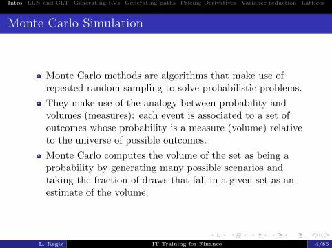
Monte Carlo Simulation

Monte Carlo methods are algorithms that make use ofrepeated random sampling to solve probabilistic problems.

They make use of the analogy between probability andvolumes (measures): each event is associated to a set ofoutcomes whose probability is a measure (volume) relativeto the universe of possible outcomes.

Monte Carlo computes the volume of the set as being aprobability by generating many possible scenarios andtaking the fraction of draws that fall in a given set as anestimate of the volume.



Monte Carlo Simulations/2

Integrals, as well as expectations, can be effectivelycomputed using Monte Carlo simulation.

The law of large numbers ensures that, when the number ofdraws is large enough, our estimates of volumes or integralsget close to their real value. The central limit theoremcontrols the speed of convergence.

They allow to tackle those problems for which no analyticalsolution is present.



Financial Applications

Study the statistical properties of portfolios: expectedreturns, risk, effectiveness of hedging strategies,...

Computing the values of derivatives, which can berepresented as expected values in a risk neutral world.



How to use Monte Carlo in Finance

Represent the relevant basic financial quantities usingmodels;

Define valuation models for more complex contracts(options/derivatives/contingent claims) that depend on thebasic quantities above;

Generate many trajectories (paths) of the possibleevolutions of the basic quantities (stocks, interest rates,exchange rates,...), also considering their relationships(dependence), defining a sufficiently large number ofscenarios.

Use the results to compute statistics of a portfolio, such asrisk measures, or to evaluate products.



What’s up next?

In the rest of our course we will:1 (Briefly) recall the principles on which MC is based on;2 (Briefly) recall how to generate random variables;3 Learn how to generate trajectories of different processes;4 Learn how to use MC to price derivatives and estimate risk

measures using variance reduction techniques.



Section

1 Introduction









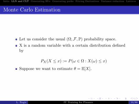
Monte Carlo Estimation

Let us consider the usual (Ω,F ,P) probability space.

X is a random variable with a certain distribution definedby

PX(X ≤ x) := P (ω ∈ Ω : X(ω) ≤ x)

Suppose we want to estimate θ = E[X].



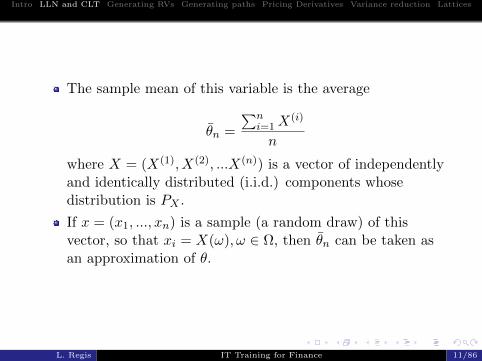
The sample mean of this variable is the average

θn =

∑ni=1X

(i)

n

where X = (X(1), X(2), ...X(n)) is a vector of independentlyand identically distributed (i.i.d.) components whosedistribution is PX .

If x = (x1, ..., xn) is a sample (a random draw) of thisvector, so that xi = X(ω), ω ∈ Ω, then θn can be taken asan approximation of θ.



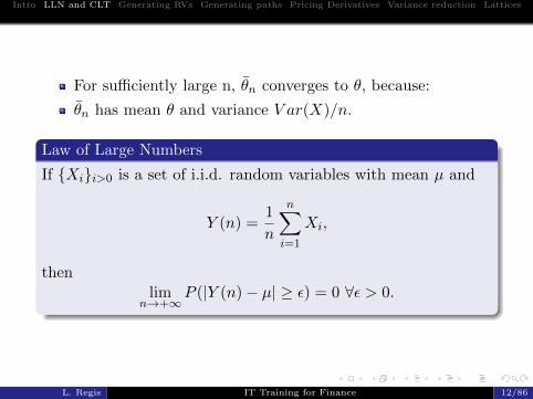
For sufficiently large n, θn converges to θ, because:

θn has mean θ and variance V ar(X)/n.

Law of Large Numbers

If Xii>0 is a set of i.i.d. random variables with mean µ and

Y (n) =1

n

n∑i=1

Xi,

thenlim

n→+∞P (|Y (n)− µ| ≥ ε) = 0 ∀ε > 0.



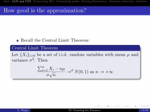
How good is the approximation?

Recall the Central Limit Theorem:

Central Limit Theorem

Let Xii>0 be a set of i.i.d. random variables with mean µ andvariance σ2. Then∑n

i=1Xi − nµσ√n

→d N(0, 1) as n→ +∞



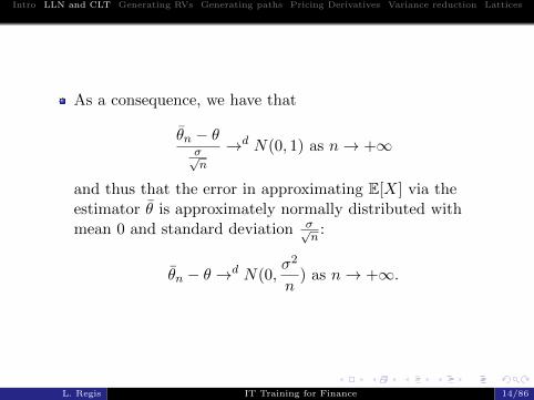
As a consequence, we have that

θn − θσ√n

→d N(0, 1) as n→ +∞

and thus that the error in approximating E[X] via theestimator θ is approximately normally distributed withmean 0 and standard deviation σ√

n:

θn − θ →d N(0,σ2

n) as n→ +∞.



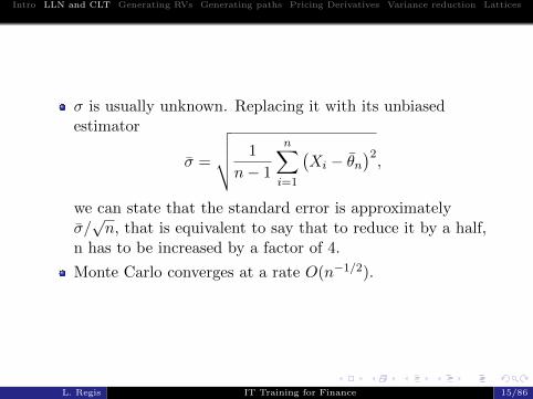
σ is usually unknown. Replacing it with its unbiasedestimator

σ =

√√√√ 1

n− 1

n∑i=1

(Xi − θn

)2,

we can state that the standard error is approximatelyσ/√n, that is equivalent to say that to reduce it by a half,

n has to be increased by a factor of 4.

Monte Carlo converges at a rate O(n−1/2).



Section

1 Introduction









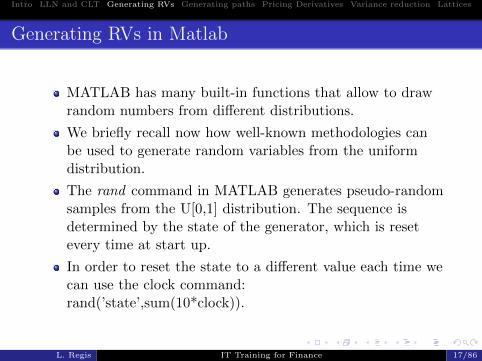
Generating RVs in Matlab

MATLAB has many built-in functions that allow to drawrandom numbers from different distributions.

We briefly recall now how well-known methodologies canbe used to generate random variables from the uniformdistribution.

The rand command in MATLAB generates pseudo-randomsamples from the U[0,1] distribution. The sequence isdetermined by the state of the generator, which is resetevery time at start up.

In order to reset the state to a different value each time wecan use the clock command:rand(’state’,sum(10*clock)).



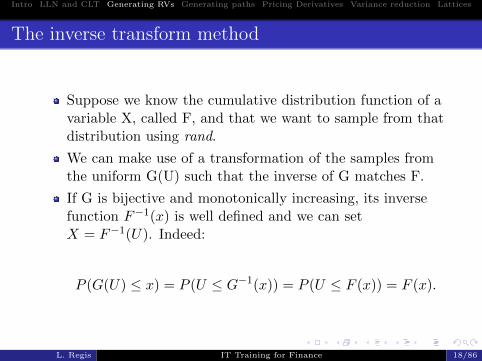
The inverse transform method

Suppose we know the cumulative distribution function of avariable X, called F, and that we want to sample from thatdistribution using rand.

We can make use of a transformation of the samples fromthe uniform G(U) such that the inverse of G matches F.

If G is bijective and monotonically increasing, its inversefunction F−1(x) is well defined and we can setX = F−1(U). Indeed:

P (G(U) ≤ x) = P (U ≤ G−1(x)) = P (U ≤ F (x)) = F (x).



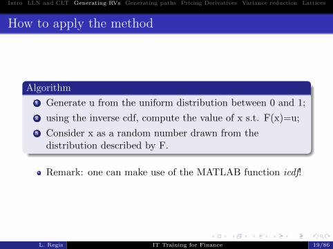
How to apply the method

Algorithm

1 Generate u from the uniform distribution between 0 and 1;

2 using the inverse cdf, compute the value of x s.t. F(x)=u;

3 Consider x as a random number drawn from thedistribution described by F.

Remark: one can make use of the MATLAB function icdf!



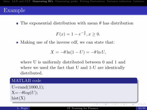
Example

The exponential distribution with mean θ has distribution

F (x) = 1− e−xθ , x ≥ 0.

Making use of the inverse cdf, we can state that:

X = −θ ln(1− U) = −θ lnU,

where U is uniformly distributed between 0 and 1 andwhere we used the fact that U and 1-U are identicallydistributed.

MATLAB code

U=rand(1000,1);X=−θlog(U);hist(X)



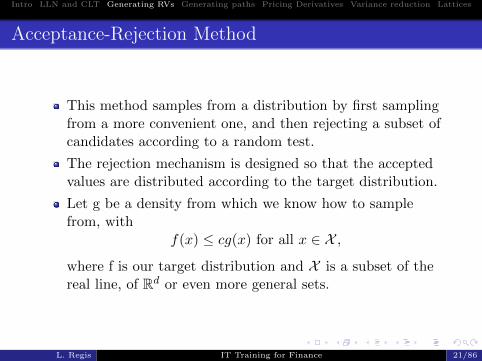
Acceptance-Rejection Method

This method samples from a distribution by first samplingfrom a more convenient one, and then rejecting a subset ofcandidates according to a random test.

The rejection mechanism is designed so that the acceptedvalues are distributed according to the target distribution.

Let g be a density from which we know how to samplefrom, with

f(x) ≤ cg(x) for all x ∈ X ,

where f is our target distribution and X is a subset of thereal line, of Rd or even more general sets.



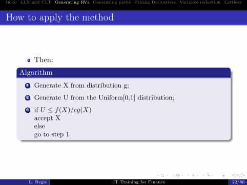
How to apply the method

Then:

Algorithm

1 Generate X from distribution g;

2 Generate U from the Uniform[0,1] distribution;

3 if U ≤ f(X)/cg(X)accept Xelsego to step 1.



Section

1 Introduction









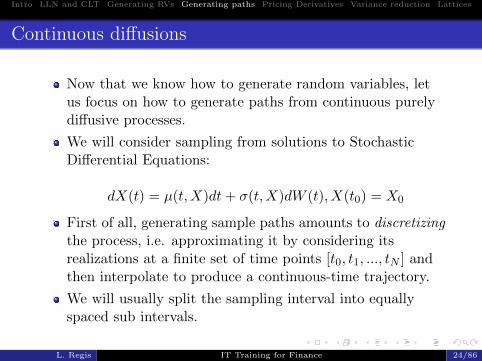
Continuous diffusions

Now that we know how to generate random variables, letus focus on how to generate paths from continuous purelydiffusive processes.

We will consider sampling from solutions to StochasticDifferential Equations:

dX(t) = µ(t,X)dt+ σ(t,X)dW (t), X(t0) = X0

First of all, generating sample paths amounts to discretizingthe process, i.e. approximating it by considering itsrealizations at a finite set of time points [t0, t1, ..., tN ] andthen interpolate to produce a continuous-time trajectory.

We will usually split the sampling interval into equallyspaced sub intervals.



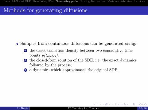
Methods for generating diffusions

Samples from continuous diffusions can be generated using:

1 the exact transition density between two consecutive timepoints p(t,x;s,y).

2 the closed-form solution of the SDE, i.e. the exact dynamicsfollowed by the process;

3 a dynamics which approximates the original SDE.



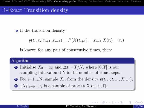
1-Exact Transition density

If the transition density

p(ti, xi; ti+1, xi+1) = P (X(ti+1) = xi+1|X(ti) = xi)

is known for any pair of consecutive times, then:

Algorithm

1 Initialise X0 = x0 and ∆t = T/N , where [0,T] is oursampling interval and N is the number of time steps.

2 For i=1,...N, sample Xi, from the density p(ti, ·; ti−1, Xi−1);

3 Xii=0,...,N is a sample of process X on [0,T].



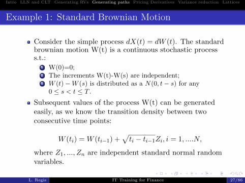
Example 1: Standard Brownian Motion

Consider the simple process dX(t) = dW (t). The standardbrownian motion W(t) is a continuous stochastic processs.t.:

1 W(0)=0;2 The increments W(t)-W(s) are independent;3 W (t)−W (s) is distributed as a N(0, t− s) for any

0 ≤ s < t ≤ T .

Subsequent values of the process W(t) can be generatedeasily, as we know the transition density between twoconsecutive time points:

W (ti) = W (ti−1) +√ti − ti−1Zi, i = 1, ....N,

where Z1, ..., Zn are independent standard normal randomvariables.



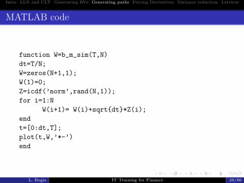
MATLAB code

function W=b_m_sim(T,N)

dt=T/N;

W=zeros(N+1,1);

W(1)=0;

Z=icdf(’norm’,rand(N,1));

for i=1:N

W(i+1)= W(i)+sqrtdt*Z(i);

end

t=[0:dt,T];

plot(t,W,’*-’)

end



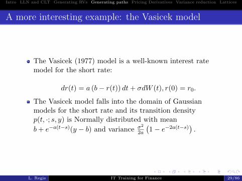
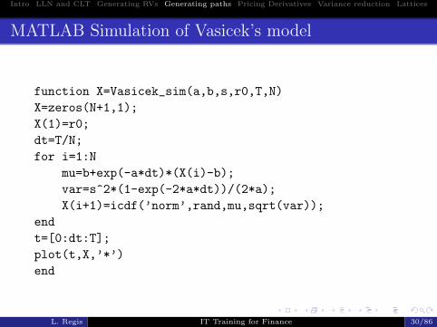
A more interesting example: the Vasicek model

The Vasicek (1977) model is a well-known interest ratemodel for the short rate:

dr(t) = a (b− r(t)) dt+ σdW (t), r(0) = r0.

The Vasicek model falls into the domain of Gaussianmodels for the short rate and its transition densityp(t, ·; s, y) is Normally distributed with mean

b+ e−a(t−s)(y − b) and variance σ2

2a

(1− e−2a(t−s)) .



MATLAB Simulation of Vasicek’s model

function X=Vasicek_sim(a,b,s,r0,T,N)

X=zeros(N+1,1);

X(1)=r0;

dt=T/N;

for i=1:N

mu=b+exp(-a*dt)*(X(i)-b);

var=s^2*(1-exp(-2*a*dt))/(2*a);

X(i+1)=icdf(’norm’,rand,mu,sqrt(var));

end

t=[0:dt:T];

plot(t,X,’*’)

end



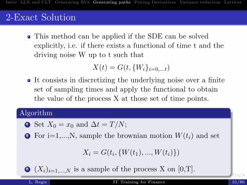
2-Exact Solution

This method can be applied if the SDE can be solvedexplicitly, i.e. if there exists a functional of time t and thedriving noise W up to t such that

X(t) = G(t, Wii=0,...t)

It consists in discretizing the underlying noise over a finiteset of sampling times and apply the functional to obtainthe value of the process X at those set of time points.

Algorithm

1 Set X0 = x0 and ∆t = T/N ;

2 For i=1,...,N, sample the brownian motion W (ti) and set

Xi = G(ti, W (t1), ...,W (ti))

3 (Xi)i=1,...,N is a sample of the process X on [0,T].



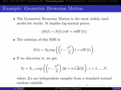
Example: Geometric Brownian Motion

The Geometric Brownian Motion is the most widely usedmodel for stocks. It implies log-normal prices.

dS(t) = S(t) (rdt+ σdW (t))

The solution of this SDE is

S(t) = S0 exp

((r − σ2

2

)t+ σW (t)

).

If we discretize it, we get:

Si = Si−1 exp

((r − σ2

2

)∆t+ σ

√∆tZi

), i = 1, ..., N.

where Zis are independent samples from a standard normalrandom variable.



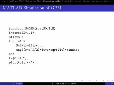
MATLAB Simulation of GBM

function S=GBM(r,s,S0,T,N)

S=zeros(N+1,1);

S(1)=S0;

for i=1:N

S(i+1)=S(i)*...

exp((r-s^2/2)*dt+s*sqrt(dt)*randn);

end

t=[0:dt:T];

plot(t,S,’*-’)



3-Approximating the dynamics

When the two previoulsy described methods are notapplicable, it is possible to simulate the solutionapproximating the dynamics of the system, i.e. by solvingthe stochastic difference equation associated to the SDE.

There are several ways of approximating, we will see themost common one, the Euler scheme.



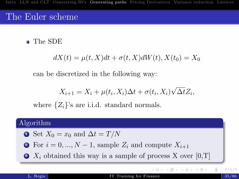
The Euler scheme

The SDE

dX(t) = µ(t,X)dt+ σ(t,X)dW (t), X(t0) = X0

can be discretized in the following way:

Xi+1 = Xi + µ(ti, Xi)∆t+ σ(ti, Xi)√

∆tZi,

where Zi’s are i.i.d. standard normals.

Algorithm

1 Set X0 = x0 and ∆t = T/N

2 For i = 0, ..., N − 1, sample Zi and compute Xi+1

3 Xi obtained this way is a sample of process X over [0,T]



Approximation Error

Being based on an approximation, the use of the Eulerscheme entails an error.

Let XEU be the approximate solution computed based onthe Euler Scheme and X the exact one. Then

E[supt∈[0,T ]|XEU (t)−X(t)|2

]≤ C∆t,

with C constant.

The approximation error is smaller the smaller ∆t.



Example: Cox, Ingersoll, Ross (1985) process

The CIR process is used in the domain of interest rates. Itis a square root process, which may never become negative:

dr(t) = a(b−X(t))dt+ σ√r(t)dW (t).

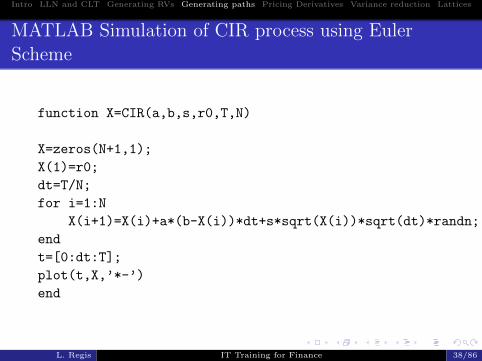
We can discretize it using the Euler Scheme as:

rt+1 = rt + a(b− rt)∆t+ σ√rt√

∆tZi,

where Zis are independent random samples from astandard normal distribution.



MATLAB Simulation of CIR process using EulerScheme

function X=CIR(a,b,s,r0,T,N)

X=zeros(N+1,1);

X(1)=r0;

dt=T/N;

for i=1:N

X(i+1)=X(i)+a*(b-X(i))*dt+s*sqrt(X(i))*sqrt(dt)*randn;

end

t=[0:dt:T];

plot(t,X,’*-’)

end



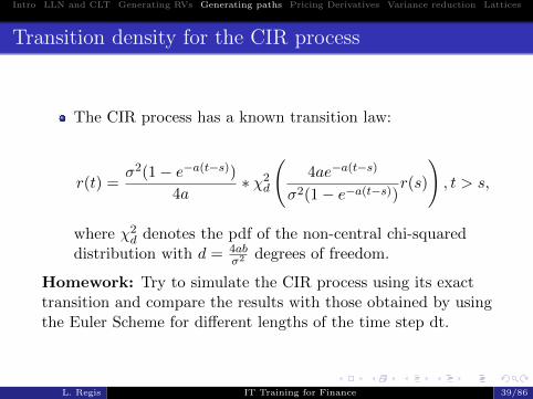
Transition density for the CIR process

The CIR process has a known transition law:

r(t) =σ2(1− e−a(t−s))

4a∗ χ2

d

(4ae−a(t−s)

σ2(1− e−a(t−s))r(s)

), t > s,

where χ2d denotes the pdf of the non-central chi-squared

distribution with d = 4abσ2 degrees of freedom.

Homework: Try to simulate the CIR process using its exacttransition and compare the results with those obtained by usingthe Euler Scheme for different lengths of the time step dt.



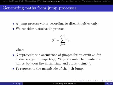
Generating paths from jump processes

A jump process varies according to discontinuities only.

We consider a stochastic process

J(t) =

N(t)∑j=1

Yj ,

where

N represents the occurrence of jumps: for an event ω, forinstance a jump trajectory, N(t, ω) counts the number ofjumps between the initial time and current time t;

Yj represents the magnitude of the j-th jump.



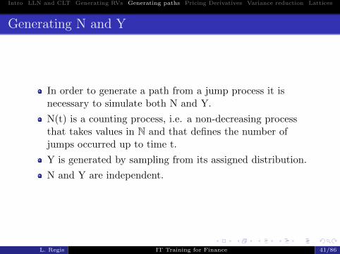
Generating N and Y

In order to generate a path from a jump process it isnecessary to simulate both N and Y.

N(t) is a counting process, i.e. a non-decreasing processthat takes values in N and that defines the number ofjumps occurred up to time t.

Y is generated by sampling from its assigned distribution.

N and Y are independent.



Simulating a counting process

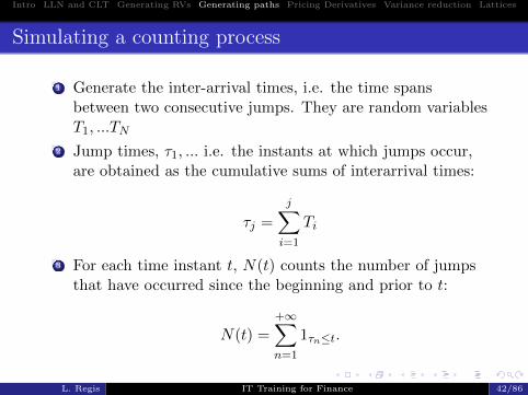
1 Generate the inter-arrival times, i.e. the time spansbetween two consecutive jumps. They are random variablesT1, ...TN

2 Jump times, τ1, ... i.e. the instants at which jumps occur,are obtained as the cumulative sums of interarrival times:

τj =

j∑i=1

Ti

3 For each time instant t, N(t) counts the number of jumpsthat have occurred since the beginning and prior to t:

N(t) =

+∞∑n=1

1τn≤t.



Example: Poisson process

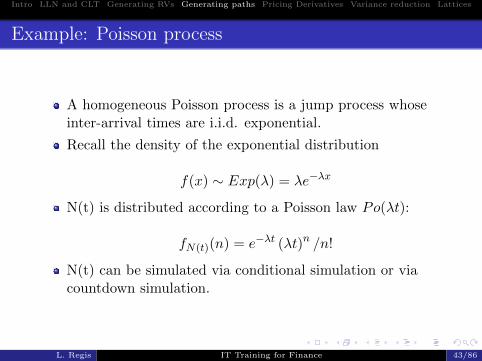
A homogeneous Poisson process is a jump process whoseinter-arrival times are i.i.d. exponential.

Recall the density of the exponential distribution

f(x) ∼ Exp(λ) = λe−λx

N(t) is distributed according to a Poisson law Po(λt):

fN(t)(n) = e−λt (λt)n /n!

N(t) can be simulated via conditional simulation or viacountdown simulation.



Simulating the counting process

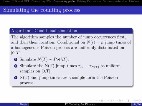
Algorithm - Conditional simulation

The algorithm samples the number of jump occurrences first,and then their location. Conditional on N(t) = n jump times ofa homogeneous Poisson process are uniformly distributed on[0, T ].

1 Simulate N(T ) ∼ Po(λT ).

2 Simulate the N(T) jump times τ1, ..., τN(T ) as uniformsamples on [0,T].

3 N(T) and jump times are a sample form the Poissonprocess.



MATLAB code

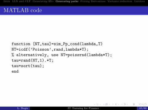
function [NT,tau]=sim_Pp_cond(lambda,T)

NT=icdf(’Poisson’,rand,lambda*T);

% alternatively, use NT=poissrnd(lambda*T);

tau=rand(NT,1).*T;

tau=sort(tau);

end



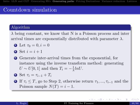
Countdown simulation

Algorithm

λ being constant, we know that N is a Poisson process and interarrival times are exponentially distributed with parameter λ.

1 Let τ0 = 0, i = 0

2 Set i = i+ 1

3 Generate inter-arrival times from the exponential, forinstance using the inverse transform method: generatingU ∼ U [0, 1] and then Ti = − 1

λ lnU .

4 Set τi = τi−1 + Ti5 If τi ≤ T , go to Step 2, otherwise return τ1, ..., τi−1 and the

Poisson sample N(T ) = i− 1.



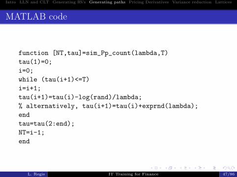
MATLAB code

function [NT,tau]=sim_Pp_count(lambda,T)

tau(1)=0;

i=0;

while (tau(i+1)<=T)

i=i+1;

tau(i+1)=tau(i)-log(rand)/lambda;

% alternatively, tau(i+1)=tau(i)+exprnd(lambda);

end

tau=tau(2:end);

NT=i-1;

end



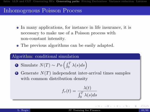
Inhomogenous Poisson Process

In many applications, for instance in life insurance, it isnecessary to make use of a Poisson process withnon-constant intensity.

The previous algorithms can be easily adapted.

Algorithm: conditional simulation

1 Simulate N(T ) ∼ Po(∫ T

0 λ(s)ds)

2 Generate N(T ) independent inter-arrival times sampleswith common distribution density

fτ (t) =λ(t)∫ T

0 λ(s)ds



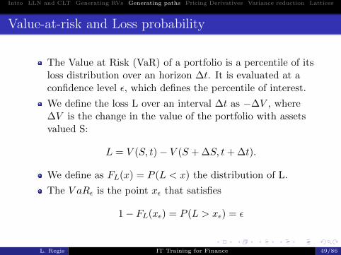
Value-at-risk and Loss probability

The Value at Risk (VaR) of a portfolio is a percentile of itsloss distribution over an horizon ∆t. It is evaluated at aconfidence level ε, which defines the percentile of interest.

We define the loss L over an interval ∆t as −∆V , where∆V is the change in the value of the portfolio with assetsvalued S:

L = V (S, t)− V (S + ∆S, t+ ∆t).

We define as FL(x) = P (L < x) the distribution of L.

The V aRε is the point xε that satisfies

1− FL(xε) = P (L > xε) = ε



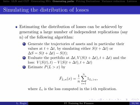
Simulating the distribution of losses

Estimating the distribution of losses can be achieved bygenerating a large number of independent replications (sayn) of the following algorithm:

1 Generate the trajectories of assets and in particular theirvalues at t+ ∆t, by simulating either S(t+ ∆t) or∆S = S(t+ ∆t)− S(t);

2 Evaluate the portfolio at ∆t, V (S(t+ ∆t), t+ ∆t) and theloss: V (S(t), t)− V (S(t+ ∆t), t+ ∆t)

3 Estimate P (L > x) by

FL,n(x) =1

n

n∑i=1

1Li>x,

where Li is the loss computed in the i-th replication.



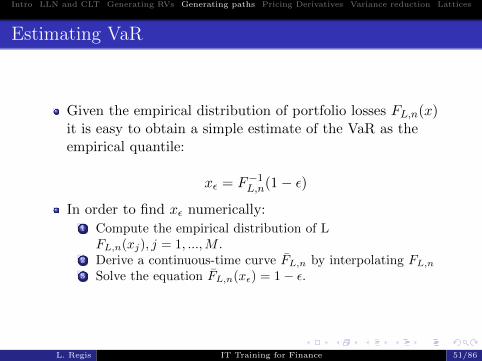
Estimating VaR

Given the empirical distribution of portfolio losses FL,n(x)it is easy to obtain a simple estimate of the VaR as theempirical quantile:

xε = F−1L,n(1− ε)

In order to find xε numerically:1 Compute the empirical distribution of LFL,n(xj), j = 1, ...,M .

2 Derive a continuous-time curve FL,n by interpolating FL,n3 Solve the equation FL,n(xε) = 1− ε.



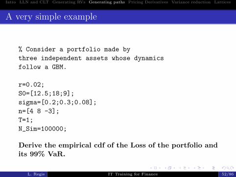
A very simple example

% Consider a portfolio made by

three independent assets whose dynamics

follow a GBM.

r=0.02;

S0=[12.5;18;9];

sigma=[0.2;0.3;0.08];

n=[4 8 -3];

T=1;

N_Sim=100000;

Derive the empirical cdf of the Loss of the portfolio andits 99% VaR.



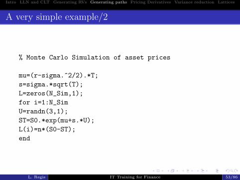
A very simple example/2

% Monte Carlo Simulation of asset prices

mu=(r-sigma.^2/2).*T;

s=sigma.*sqrt(T);

L=zeros(N_Sim,1);

for i=1:N_Sim

U=randn(3,1);

ST=S0.*exp(mu+s.*U);

L(i)=n*(S0-ST);

end



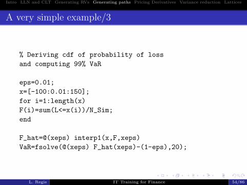
A very simple example/3

% Deriving cdf of probability of loss

and computing 99% VaR

eps=0.01;

x=[-100:0.01:150];

for i=1:length(x)

F(i)=sum(L<=x(i))/N_Sim;

end

F_hat=@(xeps) interp1(x,F,xeps)

VaR=fsolve(@(xeps) F_hat(xeps)-(1-eps),20);



Section

1 Introduction









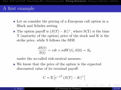
A first example

Let us consider the pricing of a European call option in aBlack and Scholes setting

The option payoff is (S(T )−K)+, where S(T) is the timeT (maturity of the option) price of the stock and K is thestrike price, while S follows the SDE

dS(t)

S(t)= rdt+ σdW (t), S(0) = S0

under the so-called risk-neutral measure.

We know that the price of the option is the expecteddiscounted value of its terminal payoff:

C = E[e−rT (S(T )−K)+]



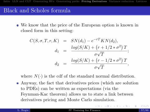
Black and Scholes formula

We know that the price of the European option is known inclosed form in this setting:

C(S, σ, T, r,K) = SN(d1)− e−rTKN(d2),

d1 =log(S/K) +

(r + 1/2 ∗ σ2

)T

σ√T

;

d2 =log(S/K) +

(r − 1/2 ∗ σ2

)T

σ√T

,

where N(·) is the cdf of the standard normal distribution.

Anyway, the fact that derivatives prices (which are solutionto PDEs) can be written as expectations (via theFeynman-Kac theorem) allows us to state a link betweenderivatives pricing and Monte Carlo simulation.



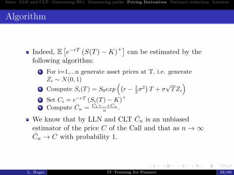
Algorithm

Indeed, E[e−rT (S(T )−K)+] can be estimated by the

following algorithm:

1 For i=1,...n generate asset prices at T, i.e. generateZi ∼ N(0, 1)

2 Compute Si(T ) = S0exp((r − 1

2σ2)T + σ

√TZi

)3 Set Ci = e−rT (Si(T )−K)

+

4 Compute Cn = C1+...+Cn

n .

We know that by LLN and CLT Cn is an unbiasedestimator of the price C of the Call and that as n→∞Cn → C with probability 1.



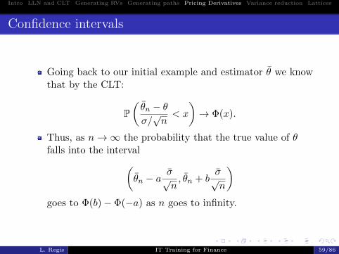
Confidence intervals

Going back to our initial example and estimator θ we knowthat by the CLT:

P(θn − θσ/√n< x

)→ Φ(x).

Thus, as n→∞ the probability that the true value of θfalls into the interval(

θn − aσ√n, θn + b

σ√n

)goes to Φ(b)− Φ(−a) as n goes to infinity.



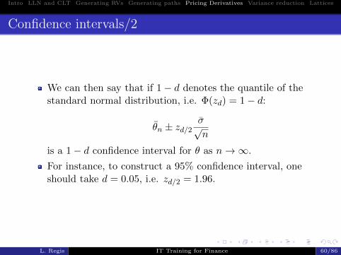
Confidence intervals/2

We can then say that if 1− d denotes the quantile of thestandard normal distribution, i.e. Φ(zd) = 1− d:

θn ± zd/2σ√n

is a 1− d confidence interval for θ as n→∞.

For instance, to construct a 95% confidence interval, oneshould take d = 0.05, i.e. zd/2 = 1.96.



CPU time, number of replications and approximationerror

Let us now write a simple piece of code that computes theexact price and Monte Carlo price of a European call, itsvariance and the CPU time with different number ofsimulations.



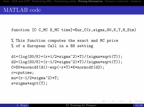
MATLAB code

function [C C_MC S_MC time]=Eur_C(r,sigma,S0,K,T,N_Sim)

% This function computes the exact and MC price

% of a European Call in a BS setting

d1=(log(S0/K)+(r+1/2*sigma^2)*T)/(sigma*sqrt(T));

d2=(log(S0/K)+(r-1/2*sigma^2)*T)/(sigma*sqrt(T));

C=S0*normcdf(d1)-exp(-r*T)*K*normcdf(d2);

c=cputime;

mu=(r-1/2*sigma^2)*T;

s=sigma*sqrt(T);



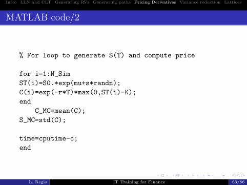
MATLAB code/2

% For loop to generate S(T) and compute price

for i=1:N_Sim

ST(i)=S0.*exp(mu+s*randn);

C(i)=exp(-r*T)*max(0,ST(i)-K);

end

C_MC=mean(C);

S_MC=std(C);

time=cputime-c;

end



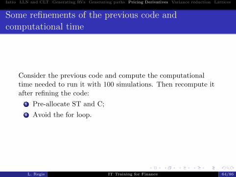
Some refinements of the previous code andcomputational time

Consider the previous code and compute the computationaltime needed to run it with 100 simulations. Then recompute itafter refining the code:

1 Pre-allocate ST and C;

2 Avoid the for loop.



Section

1 Introduction









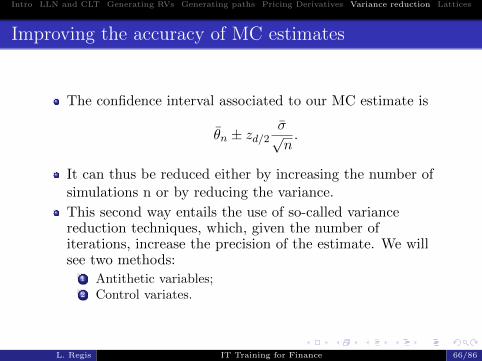
Improving the accuracy of MC estimates

The confidence interval associated to our MC estimate is

θn ± zd/2σ√n.

It can thus be reduced either by increasing the number ofsimulations n or by reducing the variance.

This second way entails the use of so-called variancereduction techniques, which, given the number ofiterations, increase the precision of the estimate. We willsee two methods:

1 Antithetic variables;2 Control variates.



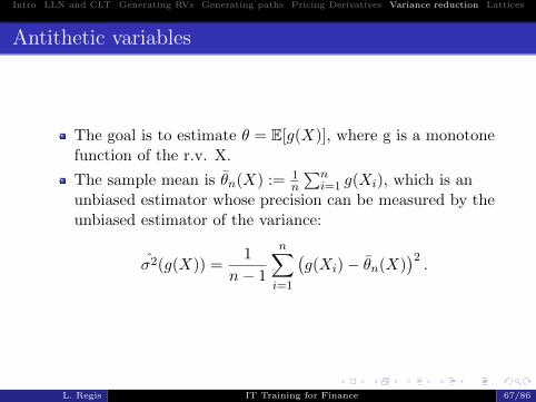
Antithetic variables

The goal is to estimate θ = E[g(X)], where g is a monotonefunction of the r.v. X.

The sample mean is θn(X) := 1n

∑ni=1 g(Xi), which is an

unbiased estimator whose precision can be measured by theunbiased estimator of the variance:

σ2(g(X)) =1

n− 1

n∑i=1

(g(Xi)− θn(X)

)2.



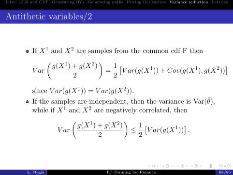
Antithetic variables/2

If X1 and X2 are samples from the common cdf F then

V ar

(g(X1) + g(X2)

2

)=

1

2

[V ar(g(X1)) + Cov(g(X1), g(X2))

]since V ar(g(X1)) = V ar(g(X2)).

If the samples are independent, then the variance is Var(θ),while if X1 and X2 are negatively correlated, then

V ar

(g(X1) + g(X2)

2

)≤ 1

2

[V ar(g(X1))

].



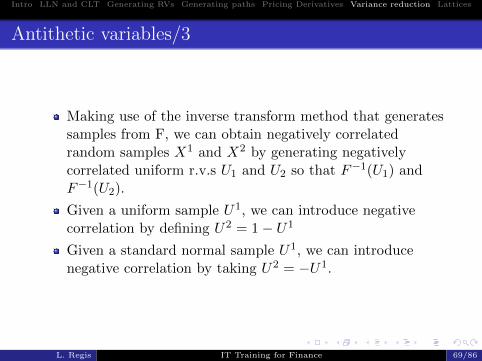
Antithetic variables/3

Making use of the inverse transform method that generatessamples from F, we can obtain negatively correlatedrandom samples X1 and X2 by generating negativelycorrelated uniform r.v.s U1 and U2 so that F−1(U1) andF−1(U2).

Given a uniform sample U1, we can introduce negativecorrelation by defining U2 = 1− U1

Given a standard normal sample U1, we can introducenegative correlation by taking U2 = −U1.



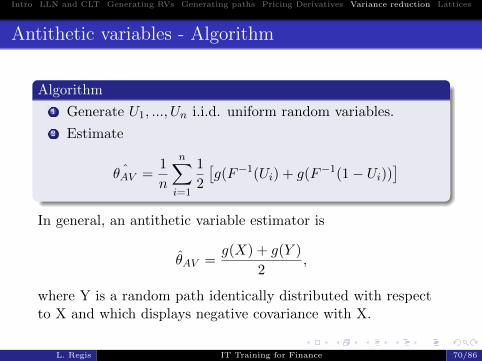
Antithetic variables - Algorithm

Algorithm

1 Generate U1, ..., Un i.i.d. uniform random variables.

2 Estimate

ˆθAV =1

n

n∑i=1

1

2

[g(F−1(Ui) + g(F−1(1− Ui))

]In general, an antithetic variable estimator is

θAV =g(X) + g(Y )

2,

where Y is a random path identically distributed with respectto X and which displays negative covariance with X.



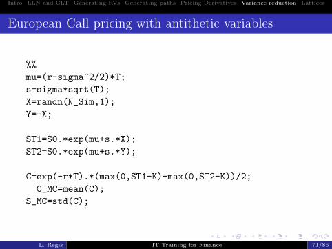
European Call pricing with antithetic variables

%%

mu=(r-sigma^2/2)*T;

s=sigma*sqrt(T);

X=randn(N_Sim,1);

Y=-X;

ST1=S0.*exp(mu+s.*X);

ST2=S0.*exp(mu+s.*Y);

C=exp(-r*T).*(max(0,ST1-K)+max(0,ST2-K))/2;

C_MC=mean(C);

S_MC=std(C);



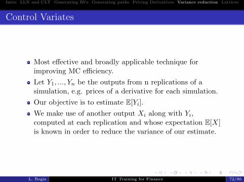
Control Variates

Most effective and broadly applicable technique forimproving MC efficiency.

Let Y1, ..., Yn be the outputs from n replications of asimulation, e.g. prices of a derivative for each simulation.

Our objective is to estimate E[Yi].

We make use of another output Xi along with Yi,computed at each replication and whose expectation E[X]is known in order to reduce the variance of our estimate.



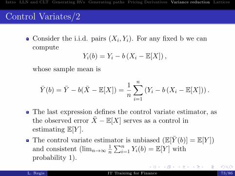
Control Variates/2

Consider the i.i.d. pairs (Xi, Yi). For any fixed b we cancompute

Yi(b) = Yi − b (Xi − E[X]) ,

whose sample mean is

Y (b) = Y − b(X − E[X]) =1

n

n∑i=1

(Yi − b (Xi − E[X])) .

The last expression defines the control variate estimator, asthe observed error X − E[X] serves as a control inestimating E[Y ].

The control variate estimator is unbiased (E[Y (b)] = E[Y ])and consistent (limn→∞

1n

∑ni=1 Yi(b) = E[Y ] with

probability 1).



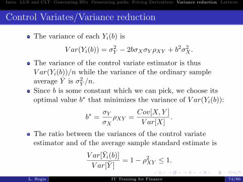
Control Variates/Variance reduction

The variance of each Yi(b) is

V ar(Yi(b)) = σ2Y − 2bσXσY ρXY + b2σ2

X .

The variance of the control variate estimator is thusV ar(Yi(b))/n while the variance of the ordinary sampleaverage Y is σ2

Y /n.

Since b is some constant which we can pick, we choose itsoptimal value b∗ that minimizes the variance of V ar(Yi(b)):

b∗ =σYσX

ρXY =Cov[X,Y ]

V ar[X].

The ratio between the variances of the control variateestimator and of the average sample standard estimate is

V ar[Yi(b)]

V ar[Y ]= 1− ρ2

XY ≤ 1.



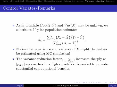
Control Variates/Remarks

As in principle Cov(X,Y ) and V ar(X) may be unkown, wesubstitute b by its population estimate:

bn =

∑ni=1

(Xi − X

) (Yi − Y

)∑ni=1

(Xi − X

)2 .

Notice that covariance and variance of X might themselvesbe estimated using MC simulation!

The variance reduction factor, 11−ρ2XY

, increases sharply as

|ρXY | approaches 1: a high correlation is needed to providesubstantial computational benefits.



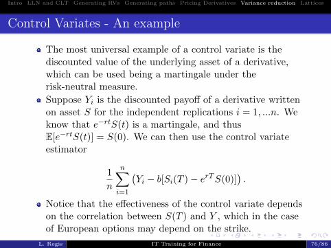
Control Variates - An example

The most universal example of a control variate is thediscounted value of the underlying asset of a derivative,which can be used being a martingale under therisk-neutral measure.

Suppose Yi is the discounted payoff of a derivative writtenon asset S for the independent replications i = 1, ...n. Weknow that e−rtS(t) is a martingale, and thusE[e−rtS(t)] = S(0). We can then use the control variateestimator

1

n

n∑i=1

(Yi − b[Si(T )− erTS(0)]

).

Notice that the effectiveness of the control variate dependson the correlation between S(T ) and Y , which in the caseof European options may depend on the strike.



Section

1 Introduction









Lattices

Lattices provide a discrete-time, discrete-spaceapproximation to the evolution of a diffusion process.

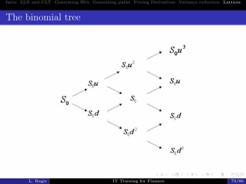
Each node in the tree is associated to a value of the asset,which is linked for each time step with successive nodes,i.e. with a set of possible future values. In the case of abinomial tree, these possible future values correspond to anup and a down move of the price.

By varying the distance between the nodes in terms ofspace and time it is possible to vary the conditional meanand variance of the change in the underlying,approximating virtually any diffusion process.

It is useful to price derivatives by backward induction,computing the payoffs at terminal nodes and then goingback.



The binomial tree



Pricing derivatives in the binomial tree

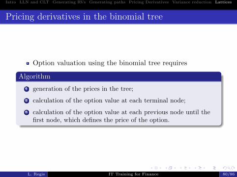
Option valuation using the binomial tree requires

Algorithm

1 generation of the prices in the tree;

2 calculation of the option value at each terminal node;

3 calculation of the option value at each previous node until thefirst node, which defines the price of the option.



Asset price generation

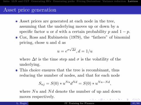
Asset prices are generated at each node in the tree,assuming that the underlying moves up or down by aspecific factor u or d with a certain probability p and 1− p.Cox, Ross and Rubinstein (1979), the “fathers” of binomialpricing, chose u and d as

u = eσ√

∆t, d = 1/u

where ∆t is the time step and σ is the volatility of theunderlying.

This choice ensures that the tree is recombinant, thusreducing the number of nodes, and that for each node

Snj = S(0) ∗ uNudNd = S(0) ∗ uNu−Nd,

where Nu and Nd denote the number of up and downmoves respectively.



Calculation of option value at final nodes

At each last node, which corresponds to the maturity ofthe option, the payoff of the option, i.e. its exercise value,must be calculated.

For instance, for a European call, the value of the option ateach terminal node n, j will be

max(Sn,j −K, 0),

where K is the strike price and Sn,j denotes the asset priceat the j-th final node.



Calculation of option value at each node

For each node, going backwards from the next to last tothe first, we compute the risk-neutral value of the option.

Following the risk-neutral approach, the fair price of aderivative is the expected discounted value of its futurepayoff.

At each node, the expected value is computed by averagingthe values of the two following nodes weigthed by theirprobabilities and discounting them at rate r.



Cox, Ross, Rubinstein and risk-neutrality

Risk-neutrality in the CRR framework requires

q =er∆t − du− d

,

and the value of a derivative at each node becomes

fj = e−r∆t (qfu,j+1 + (1− q) ∗ fd,j+1) ,

where fu and fd define the price of the derivative in case ofa successive upward or downward move respectively.



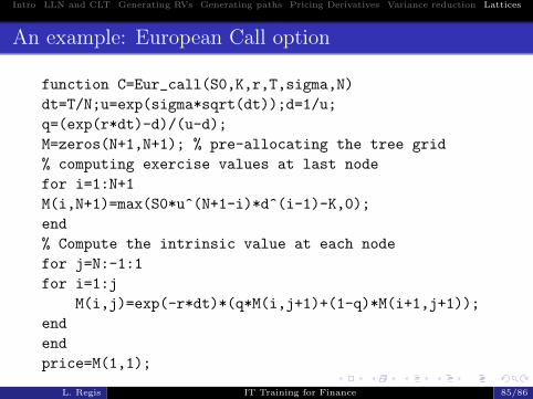
An example: European Call option

function C=Eur_call(S0,K,r,T,sigma,N)

dt=T/N;u=exp(sigma*sqrt(dt));d=1/u;

q=(exp(r*dt)-d)/(u-d);

M=zeros(N+1,N+1); % pre-allocating the tree grid

% computing exercise values at last node

for i=1:N+1

M(i,N+1)=max(S0*u^(N+1-i)*d^(i-1)-K,0);

end

% Compute the intrinsic value at each node

for j=N:-1:1

for i=1:j

M(i,j)=exp(-r*dt)*(q*M(i,j+1)+(1-q)*M(i+1,j+1));

end

end

price=M(1,1);



Useful references

P. Brandimarte, 2006, Numerical methods in finance andeconomics: a MATLAB-based introduction, John Wiley &Sons.

P. Glasserman, 2003, Monte Carlo Methods in FinancialEngineering, Spinger.

D. Higham, Nine Ways to implement the binomial methodfor option valuation in MATLAB, SIAM Review.

Cox, J., Ross, S., and Rubinstein, M., 1979, OptionPricing: a simplified approach, Journal of FinancialEconomics 7, 229-263.


Documents

Monte Carlo Simulation and Binomial Pricing with MATLABlucaregis.altervista.org/IT_Monte_Carlo.pdf · Monte Carlo Simulation Monte Carlo methods are algorithms that make use of repeated