Embed Size (px)
Citation preview

Monopoly Sale of a Network Good∗
Masaki Aoyagi†
Osaka University
September 25, 2010
Abstract
This paper studies the problem of a monopolist who sells a network goodthrough a price posting scheme. The scheme posts a price of every possibleallocation for each buyer, who are then asked to report their private informationto the seller. The seller then implements the allocation based on the reports.The social choice functions that are ex post implementable through such asales scheme are characterized, and the conditions are identified under whichthe revenue maximizing scheme has the property that the price of a largernetwork is more affordable than that of a smaller network.Key words: network externalities, ex post equilibrium, revenue maximization.Journal of Economic Literature Classification Numbers: C72, D82.
1 Introduction
Goods have network externalities when their value to any consumer depends onthe consumption decision of other consumers. A classical example of a good withnetwork externalities, or more simply a network good, is a telecommunication devicewhose value depends directly on the number of other people using the device. Otherleading examples of network goods include the operating system (OS) of PC’s, fuel-cell vehicles, social networking services, industrial parks, and so on. The nature ofnetwork externalities may be purely physical as in the case of the telecommunicationdevice, but may also be market-based or psychological. Market-based externalitiesarise when more users of a good induces the market to provide complementary goods
∗I am very grateful to Shigehiro Serizawa and Tatsuhiro Shichijo for helpful comments. Financial
support from the JSPS via grant #21653016 is gratefully acknowledged.†ISER, Osaka University, 6-1 Mihogaoka, Ibaraki, Osaka 567-0047, Japan.
1

that enhance the value of the good. More users of a fuel-cell vehicle, for example,encourages entry into the market of charge stations, which leads to the increasedvalue of such vehicles. On the other hand, much of bandwagon consumption inthe fashion, toy and electronic industries can be explained through psychologicalexternalities where consumers’ tastes for a particular good are directly influencedby the size of its consumption. When all types of externalities are accounted for, itwould be no exaggeration to say that a substantial fraction of consumption goodshave network properties.
Despite their importance, network goods have received relatively little attentionin economic theory.1 Analysis of network goods in the literature has mostly beenfocused on the resolution of the coordination problem arising from the multiplicityof equilibria. When every consumer expects others to adopt the good, its expectedvalue is high enough to render adoption a rational decision (at least for some price).On the other hand, when every consumer expects no other consumers to adopt,then its low expected value makes no adoption rational. Expectation is self-fulfillingin both cases, leading to multiple, Pareto-ranked equilibria. A subsidy schemeas proposed by Dybvig and Spatt (1983) is one way to eliminate the problem bypromising to compensate the adopters when the number of adoptions is below somethreshold. The existence of Pareto-ranked equilibria is also the main focus of theanalysis of intertemporal patterns of adoption of a network good.2 In contrast, theproblem of revenue maximization by a monopolist has been analyzed only partiallyeither through the analysis of subsidy schemes under the implicit assumption thathigher participation implies higher revenue, or through the analysis of introductoryprices, a common practice of setting a low price for early adopters and a higher,regular price for others.3 In contrast, our objective in this paper is to directly explorethe revenue maximization problem in the incomplete information environment.
In the present context, an allocation is the list of all buyers’ adoption/non-adoption decisions. Each buyer i’s valuation function vi depends on an allocation,and also is an increasing function of his private signal distributed over the unitinterval. A price-posting scheme is described as follows: The seller first posts aprice of every possible allocation for each buyer. The buyers then report theirprivate signals to the seller. An allocation is determined by the reports through
1Rofles (1974) is the first to give a theoretical analysis of network goods.2See Gale (1995, 2001), Ochs and Park (2009) and Shichijo and Nakayama (2009).3See Cabral et al. (1999). Sekiguchi (2009) examines the monopolist’s revenue in the dynamic
setup as in Gale (1995) when the price is held constant over time and across consumers.
2

an allocation rule, and offered to the buyers at the originally posted price. Finally,each buyer who is supposed to adopt in the proposed allocation chooses whether toaccept the offer or not.4
We analyze a revenue maximizing price posting scheme that is strategy-proofand ex post individually rational. Our analysis focuses on the “regularity” propertydefined as follows: We say that for buyer i, price p of an allocation a is moreaffordable than price p′ of allocation a′ if for some signal si, i’s valuation of a is abovep but his valuation of a′ is below p′. In other words, buyer i is willing to accept a
at p whenever he is willing to accept a′ at p′. A price-posting scheme is regular if(1) whenever allocation a is larger than allocation a′ (i.e., a has more adopters thana′), the price of a is more affordable than the price of a′ for every buyer, and (2) theallocation rule chooses the largest allocation as permitted by individual rationality.When the buyers’ private signals are independently distributed, we find that theoptimal scheme is regular when there are only two buyers. For a general numberof ex ante symmetric buyers, we demonstrate the optimality of a regular schemeamong the class of symmetric schemes when the externalities are sufficiently strong.We also show that a regular scheme is coalitionally strategy-proof in the sense thatno group deviations are profitable, and that there exists a regular scheme that isoptimal among the class of symmetric coalitionally strategy-proof schemes. Thelatter findings indicate the robustness of the optimality of a regular price-postingscheme against buyer collusion.5
The idea of price-posting schemes is most closely related to the concept of aninducement scheme proposed by Park (2004). An inducement scheme, which is itselfa generalization of the subsidy schemes discussed above to the incomplete informa-tion environment, is a sales mechanism in which the transfer between the seller andbuyers depends on the final allocation. We may think of an inducement scheme asfirst posting a price of each allocation, and then letting the buyers simultaneouslydecide whether to adopt or not. Hence, an inducement scheme is a subclass of price-
4In the sense that the adopters may be a subset of agents, the network good problem is related
to the problem of excludable public goods, where agents can be excluded from the use of the good.
However, the value of the public good depends on the amount of contributions from the agents
rather than their adoption decisions, and the focus of analysis is on the efficient cost sharing rather
than revenue maximization. See, for example, Moulin (1994), Deb and Razzolini (1999a, b), and
Bag and Winter (1999).5For example, potential buyers of an industrial park may be from the same industry and know
each other well.
3

posting schemes in which the buyers’ adoption decisions are made independently ofone another. In contrast, a price-posting scheme coordinates their decisions throughthe reported signal profile.
The paper is organized as follows: The next section introduces a price postingscheme. Ex post implementable schemes are characterized in Section 3. We studythe problem with two buyers in Section 4, and optimal symmetric schemes with ageneral number of ex ante symmetric buyers in Sections 5 and 6. Section 5 analyzesthe case of strong externalities, and Section 6 analyzes coalitionally strategy-proofschemes. We conclude in Section 7. All the proofs are collected in the Appendix.
2 Model
There are I potential buyers of a network good indexed by i ∈ I = {1, . . . , I}.Buyer i’s decision is either to buy the good (ai = 1), or not (ai = 0). An allocation(or a network) is a profile of adoption decisions a = (ai)i∈I , and an element of theset A = {0, 1}I . Let Ai be the set of allocations in which buyer i buys the good:Ai = {a ∈ A : ai = 1}. The value of the good to buyer i, denoted vi(a, si), dependson the allocation a as well as his own private signal si. The signal profile s = (si)i∈I
has a strictly positive joint density g over S =∏
i∈I Si, where Si is the unit interval[0, 1] ⊂ R+.
A social choice function determines the allocation of the good and monetarytransfer from each buyer as a function of the private signal profile. Formally, asocial choice function is a pair (f, τ) of an allocation rule f : S → A and a transferrule τ = (τ1, . . . , τI) : S → RI : f(s) ∈ A is the allocation under the signal profiles ∈ S, and τi(s) ∈ R is the monetary transfer from buyer i under s. A social choicefunction (f, τ) is strategy-proof if
vi(f(si, s−i), si) − τi(si, s−i) ≥ vi(f(s′i, s−i), si) − τi(s′i, s−i)
for every i, si, s′i and s−i,
and ex post individually rational if
vi(f(si, s−i), si) − τi(si, s−i) ≥ 0 for any i, si, and s−i.
A social choice function (f, τ) is ex post implementable if it is both strategy-proofand ex post individually rational.
Given the concern for the multiplicity of equilibria in the network good problems,strategy-proofness is a particularly suitable requirement compared with Bayesian
4

incentive compatibility, which does not address the multiplicity issue.6 Ex post in-dividual rationality also adequately handles the possibility of withdrawal by a buyerafter they update the value of the good upon learning the seller’s recommendation.7
The social choice function (f, τ) is simple if for any s, s′ ∈ S, f(s) = f(s′) impliesτ(s) = τ(s′). Under a simple social choice function, hence, the transfer depends onthe signal profile only through the allocation. When (f, τ) is simple, we express itas (f, t), where t : A → RI is a function of the allocation a. A price posting schemeis a mechanism described as follows: For every buyer i and every allocation a ∈ A,the seller first posts price ti(a) charged to buyer i when allocation a is realized.Facing the price schedule, the buyers report their private signals to the seller. Theseller then determines and announces the allocation f(s) ∈ A as a function of thereport profile s. Finally, every buyer i responds by either accepting or rejectingthe proposed allocation. When any buyer rejects, no transaction takes place andevery buyer receives the reservation utility of zero. Formally, a price posting schemecan be described by (S, {0, 1}I , f, t), where S is the set of message profiles, {0, 1} isthe set of each buyer’s decisions to accept (di = 1) or reject (di = 0) the proposedallocation, t = (ti(a))a∈A, i∈I is the posted price schedule, and f = (fi)i∈I : S → A
is the allocation rule.A strategy for buyer i in the price-posting mechanism is a pair (ρi, σi), where
ρi : Si → Si determines the reported signal given his true signal si, and σi : Si×A →{0, 1} determines whether to accept or reject the proposed allocation as a functionof the proposal a and the own signal si. The participation strategy (ρ∗i , σ
∗i ) of buyer
i is honest and obedient if ρ∗i (si) = si and σ∗i (si, a) = ai for every si ∈ Si and a ∈ A.
Note in particular that buyer i cannot adopt if the proposed allocation f(s) /∈ Ai.The profile of the honest and obedient strategies (ρ∗, σ∗) is an ex post equilibrium if
vi(f(si, s−i), si) − ti(f(si, s−i)) ≥ max{
maxs′i∈Si
vi(f(s′i, s−i), si) − ti(f(s′i, s−i)), 0}
for every i, si, and s−i.
6Park (2004) presents an analysis of Bayesian implementable sales mechanisms for a network
good.7That is, when buyer i with signal si has reported si and is recommended to adopt for the
payment of xi, his updated utility equals
Es−i [vi(f(si, s−i), si) − xi | si, fi(si, s−i) = 1, τi(si, s−i) = xi].
Ex post IR guarantees that the above is non-negative whereas interim IR condition
Es−i [vi(f(si, s−i), si) − τi(si, s−i) | si] ≥ 0 does not.
5

The first term in the parentheses on the right-hand side corresponds to i’s payoffwhen he makes a false report and then accepts the proposed allocation, and thesecond term to his payoff when he rejects the proposal. The following result isimmediate.
Proposition 1 Let (f, t) be a simple social choice function. Then (f, t) is ex postimplementable if and only if honesty and obedience is an ex post equilibrium of theprice posting scheme (S, {0, 1}I , f, t).
This proposition allows us to identify a simple ex post implementable socialchoice function with a price posting scheme that has honesty and obedience as anex post equilibrium. In what follows, hence, we call such a social choice function(f, t) an ex post implementable price posting scheme.
As seen, a price-posting scheme determines the price of the good only as afunction of the publicly observable final allocation. As such, it leaves little room forthe seller to deviate from his announced mechanism compared with more generalmechanisms in which the transfer may vary with the reports even when the allocationis the same.8 Let the seller’s expected revenue per buyer under a price postingscheme (f, t) be defined by
R(f, t) =1I
∑i∈I
Es[ti(f(s))].
An ex post implementable price posting scheme (f, t) is optimal if it maximizes theseller’s expected revenue:
R(f, t) = max {R(f ′, t′) : (f ′, t′) is simple and ex post implementable}.
3 Characterization of Ex Post Implementability
In this section, we present a basic characterization of ex post implementabilitythat will later be used in the analysis of optimal schemes. We make the followingassumptions on the valuation function vi : A × Si → R+:
Assumption 1 For any i ∈ I and a ∈ A,8Suppose that buyer i’s payment is higher when some other buyer j reports sj than when he
reports s′j . Since j’s report is privately solicited by the seller and unknown to i, the seller may
pretend to i that j has reported sj when in fact he reported s′j in order to demand the higher
payment. A similar problem arises in a sealed-bid second-price auction.
6

1. vi(a, 0) = 0,
2. a /∈ Ai ⇒ vi(a, ·) ≡ 0,
3. a ∈ Ai ⇒ ∂vi∂si
(a, ·) > 0,
4. vi(a, ·) = vi(b, ·) ⇒ ∂vi∂si
(a, ·) > ∂vi∂si
(b, ·) or ∂vi∂si
(b, ·) > ∂vi∂si
(a, ·).
That is, the value of the good equals zero (1) to a buyer at the lowest margin,and (2) to a non-adopter. Moreover, (3) the value is strictly increasing with theprivate signal, and (4) when the two allocations are not equivalent to any buyer, therate of increase in his value is strictly higher for one of them. We introduce somenotation as follows. First, let
Ci(a) = {a′ ∈ A : vi(a′, ·) = vi(a, ·)}
be the set of allocations among which buyer i is indifferent. For example, whenthe level of externalities depends only on the size of an allocation defined by |a| =∑
i∈I ai, then Ci(a) = {a′ ∈ Ai : |a′| = |a|} for a ∈ Ai. Next, fix any s−i ∈ S−i andlet
Bi(s−i) = {f(si, s−i) : si ∈ Si}be the set of possible allocations that buyer i can achieve by changing his reportwhen the signal profile of other buyers is fixed at s−i. Further, for any allocationa ∈ A and profile s−i ∈ S−i, let
Li(a, s−i) = cl {si ∈ Si : f(si, s−i) = a}
be the (closure of the) set of i’s signals that would lead to allocation a when others’signal profile is fixed at s−i, and for any allocation a ∈ A,
La = cl {s ∈ S : f(s) = a}
be the (closure of the) set of signal profiles that induce allocation a.Now suppose that (f, t) is a price-posting scheme. Given any allocation a ∈ Ai,
define yai ∈ [0, 1] to be the marginal signal at which buyer i is indifferent between
accepting allocation a at price ti(a), and not accepting:
vi(a, yai ) − ti(a) = 0.
7

Such a signal yai is unique by Assumption 1 if it exists. If vi(a, 0) − ti(a) > 0, then
let yai = 0 and if vi(a, 1) − ti(a) < 0, then let ya
i = 1. Likewise, given any pair ofallocations a, b ∈ Ai such that vi(a, ·) > vi(b, ·), define yab
i = ybai ∈ [0, 1] to be the
marginal signal at which buyer i is indifferent between allocation a at price ti(a)and allocation b at price ti(b):
vi(a, yabi ) − ti(a) = vi(b, yab
i ) − ti(b). (1)
Again, such a signal yabi is unique if it exists. If vi(a, 0) − ti(a) > vi(b, 0) − ti(b), set
yabi = 0 and if vi(a, 1) − ti(a) < vi(b, 1) − ti(b), set yab
i = 1.For each i ∈ I and a ∈ Ai, we may restrict attention to the price ti(a) such that
0 ≤ ti(a) ≤ vi(a, 1). Since there is a one-to-one correspondence between ti(a) andya
i for any such ti(a), we will interchangeably use the profile y = (yai )i∈I,a∈Ai and
the transfer rule t in what follows.
Proposition 2 A price posting scheme (f, t) is ex post implementable if and only ifthe following holds. For any i and s−i, if a1, . . . , an ∈ A are all distinct allocationssuch that
1. ∂vi∂si
(a1, ·) < · · · < ∂vi∂si
(an, ·), and
2. {a1, . . . , an} ⊂ Bi(s−i) ⊂⋃n
k=1 Ci(ak),
then for k = 1, . . . , n,
1. ti(a) = ti(ak) if a ∈ Ci(ak) ∩ Bi(s−i),
2. ti(a1) ≤ 0,
3. ti(a1) ≤ · · · ≤ ti(an).
4.⋃
a∈Ci(ak)∩Bi(s−i)
Li(a, s−i) =[yak−1ak
i , yakak+1
i
], where ya0a1
i = 0.
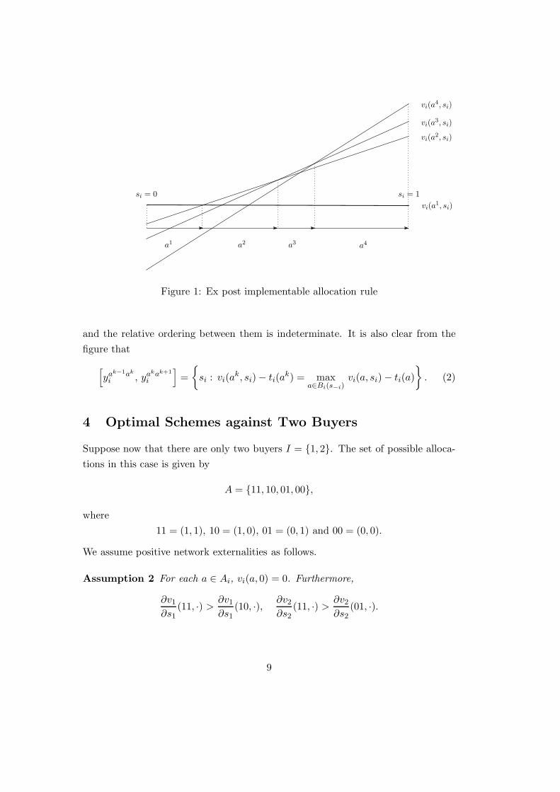
The above proposition can be illustrated as follows: Fix the signal profile ofbuyers other than i. The allocations that may be chosen for different reports ofi’s signal should be lined up in the order of the marginal values ∂vi
∂si(a, si): The
allocation a with the kth smallest ∂vi∂si
(a, si) is chosen for the kth partition intervalof reports. (Figure 1). Any two allocations with the same ∂vi
∂siare equivalent to i,
8
a1 a4a3a2
vi(a2, si)
vi(a3, si)
vi(a4, si)
vi(a1, si)si = 0 si = 1
Figure 1: Ex post implementable allocation rule
and the relative ordering between them is indeterminate. It is also clear from thefigure that[
yak−1ak
i , yakak+1
i
]=
{si : vi(ak, si) − ti(ak) = max
a∈Bi(s−i)vi(a, si) − ti(a)
}. (2)
4 Optimal Schemes against Two Buyers
Suppose now that there are only two buyers I = {1, 2}. The set of possible alloca-tions in this case is given by
A = {11, 10, 01, 00},
where11 = (1, 1), 10 = (1, 0), 01 = (0, 1) and 00 = (0, 0).
We assume positive network externalities as follows.
Assumption 2 For each a ∈ Ai, vi(a, 0) = 0. Furthermore,
∂v1
∂s1(11, ·) >
∂v1
∂s1(10, ·), ∂v2
∂s2(11, ·) >
∂v2
∂s2(01, ·).
9

The following theorem characterizes the optimal schemes in a general environ-ment with two buyers.
Theorem 1 If (f, t) is an optimal ex post implementable price posting schemeagainst two buyers under Assumption 2, then it takes one of the following forms.
(A) y111 , y11
2 < 1, y101 , y01
2 ∈ (0, 1),
⎧⎪⎪⎪⎨⎪⎪⎪⎩
(A0) y111 ≤ y10
1 , y112 ≤ y01
2
(A1) y111 ≤ y10
1 , y112 > y01
2 ,
(A2) y111 > y10
1 , y112 ≤ y01
2⎧⎪⎨⎪⎩
L11 = [y111 , 1] × [y11
2 , 1]L10 = [y10
1 , 1] × [0, y112 ]
L01 = [0, y111 ] × [y01
2 , 1].
(B1) 0 < y101 < y11
1 < y11,101 < 1, y11
2 < 1, y012 ∈ (0, 1),⎧⎪⎨
⎪⎩L11 = [y11,10
1 , 1] × [y112 , 1]
L10 = [y101 , 1] × [0, 1] \ int L11
L01 = [0, y101 ] × [y01
2 , 1].
(B2) 0 < y012 < y11
2 < y11,012 < 1, y10
1 ∈ (0, 1), y111 < 1,⎧⎪⎨
⎪⎩L11 = [y11
1 , 1] × [y11,012 , 1]
L10 = [y101 , 1] × [0, y01
2 ]L01 = [0, 1] × [y01
2 , 1] \ int L11.
(C1) y101 < y11
1 < 1, 0 < y012 < y11
2 < 1,⎧⎪⎨⎪⎩
L11 = [y111 , 1] × [y11
2 , 1]L10 = [y10
1 , 1] × [0, y112 ]
L01 = [0, y101 ] × [y01
2 , 1].
(C2) 0 < y101 < y11
1 < 1, y012 < y11
2 < 1,⎧⎪⎨⎪⎩
L11 = [y111 , 1] × [y11
2 , 1]L10 = [y10
1 , 1] × [0, y012 ]
L01 = [0, y111 ] × [y01
2 , 1].
These configurations are depicted in Figures 2, 3 and 4. As seen, an optimalscheme permits various allocation rules. Which one of these is optimal depends onthe specific distribution of signal profiles.
10

y111 y10
1
y112
y012
11
1000
01
y111 y10
1
y012
y112
11
1000
01
Figure 2: Configurations (A0) (left) and (A1) (right)
y11,101y10
1
y112
y012
11
1000
01
y111 y10
1
y11,012
y012
11
1000
01
Figure 3: Configurations (B1) (left) and (B2) (right)
y111y10
1
y112
y012
11
1000
01
y111y10
1
y112
y012
11
1000
0100
00
Figure 4: Configurations (C1) (left) and (C2) (right)
11
r1(11, s1)
r1(10, s1)
s1 = 0 s1 = 1z111 z10
1
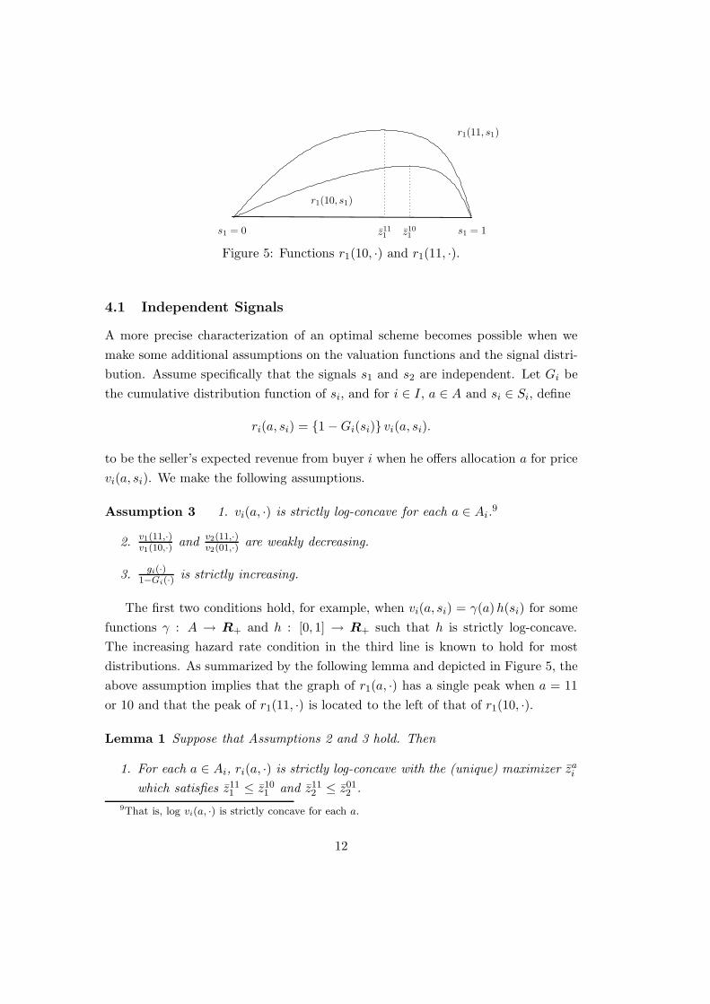
Figure 5: Functions r1(10, ·) and r1(11, ·).
4.1 Independent Signals
A more precise characterization of an optimal scheme becomes possible when wemake some additional assumptions on the valuation functions and the signal distri-bution. Assume specifically that the signals s1 and s2 are independent. Let Gi bethe cumulative distribution function of si, and for i ∈ I, a ∈ A and si ∈ Si, define
ri(a, si) = {1 − Gi(si)} vi(a, si).
to be the seller’s expected revenue from buyer i when he offers allocation a for pricevi(a, si). We make the following assumptions.
Assumption 3 1. vi(a, ·) is strictly log-concave for each a ∈ Ai.9
2. v1(11,·)v1(10,·) and v2(11,·)
v2(01,·) are weakly decreasing.
3. gi(·)1−Gi(·) is strictly increasing.
The first two conditions hold, for example, when vi(a, si) = γ(a)h(si) for somefunctions γ : A → R+ and h : [0, 1] → R+ such that h is strictly log-concave.The increasing hazard rate condition in the third line is known to hold for mostdistributions. As summarized by the following lemma and depicted in Figure 5, theabove assumption implies that the graph of r1(a, ·) has a single peak when a = 11or 10 and that the peak of r1(11, ·) is located to the left of that of r1(10, ·).
Lemma 1 Suppose that Assumptions 2 and 3 hold. Then
1. For each a ∈ Ai, ri(a, ·) is strictly log-concave with the (unique) maximizer zai
which satisfies z111 ≤ z10
1 and z112 ≤ z01
2 .9That is, log vi(a, ·) is strictly concave for each a.
12

2.
∂r1
∂s1(11, s1) <
∂r1
∂s1(10, s1) for s1 > z10
1 ,
∂r2
∂s2(11, s2) <
∂r2
∂s2(01, s2) for s2 > z01
2 .
We say that a price posting scheme (f, t) against two buyers is regular if
1. y111 ≤ y10
1 , y112 ≤ y01
2 , and
2. f1(s) =
⎧⎨⎩1 if s1 ≥ y10
1 , or s ≥ (y111 , y11
2 ),
0 otherwise,and
f2(s) =
⎧⎨⎩1 if s2 ≥ y01
2 , or s ≥ (y111 , y11
2 ),
0 otherwise.
Under a regular scheme, hence, the price of a larger network a = 11 is moreaffordable than that of a smaller network a = 10 or 01, and the network size ismaximized subject to the individual rationality constraints. The second propertycan also be interpreted as saying that the good is allocated to a single buyer onlywhen the other buyer’s signal is too low for joint adoption. Configuration (A0)in Figure 1 corresponds to a regular scheme. If a regular scheme is optimal, then(y10
1 , y012 ) = (z10
1 , z012 ) and
(y111 , y11
2 ) ∈ argmax {1 − G2(y112 )} r1(11, y11
1 ) + {1 − G1(y111 )} r2(11, y11
2 )
+ G2(y112 ) r1(10, z10
1 ) + G1(y111 ) r2(01, z01
2 ).(3)
Theorem 2 Suppose that (s1, s2) is independent. If (f, t) is an optimal ex postimplementable price posting scheme against two buyers under Assumptions 2 and 3,then it is regular.
Proof. See the Appendix.When y11
1 < y101 and y11
2 < y012 , it is impossible to replicate the allocation rule f
of a regular scheme by any scheme in which the buyers’ decisions are based only ontheir own signals or on the decisions of other buyers: In any such scheme, at leastone buyer’s decision (e.g, the first-mover’s decision) must be independent of otherbuyers’ signals.
13
Example: Suppose that si has the uniform distribution Gi(si) = si, and that thebuyers’ valuation functions are given by
v1(10, s1) = γs1
v1(11, s1) = δs1,
v2(01, s2) = γs2
v2(11, s2) = δs2,
where 0 < γ < δ. Given that the optimal scheme is regular, the marginal valuefor the single adoption 10 or 01 equals y10
1 = y012 = 1
2 . By (3) and symmetry, themarginal value y11
1 = y112 for the joint adoption 11 solves
y111 = y11
2 ∈ argmaxx
δx(1 − x)2 +γ
4x.
Solving this, we get10
y111 = y11
2 =13δ
{2δ −
√δ2 − 3
4γδ
}.
We can confirm that y111 = y11
2 < 12 = y10
1 = y012 if and only if γ < δ. Consider now
the price of each allocation associated with these marginal values. They are givenby
t1(10) = t2(01) =γ
2, and t1(11) = t2(11) =
13
{2δ −
√δ2 − 3
4γδ
}.
From these, we can check that the price of the size 2 network 11 is higher than thatof the size 1 network if and only if
δ
γ>
34.
In other words, when the network externalities are strong, the actual price of thelarger network is higher than that of the smaller network, and vice versa.
5 Optimal Symmetric Schemes
With more than two buyers, the problem of identifying all the ex post implementableschemes becomes intractable. In this section, we focus on an optimal symmetricscheme when the buyers are ex ante symmetric. We show that the optimal scheme
10As seen, the explicit derivation of the marginal values is possible only under very limited
specifications of the distribution and values.
14
is regular when the network externalities are strong, or when a stronger notion ofincentive compatibility is imposed.
Suppose that the signals s1, . . . , sI are independent and identically distributed,and denote by g the density of si and by G the corresponding cumulative distribu-tion. The valuation functions are symmetric in the sense that
vi(a, s) = vj(a, s′)
for any a ∈ A, i = j, and s, s′ ∈ S such that (si, sj , s−i−j) = (s′j, s′i, s−i−j). The
symmetry condition implies that the network externalities depend only on the sizeof the allocation a ∈ A, defined by |a| =
∑j∈I aj. For this reason, we denote by
vn : [0, 1] → R+ the valuation function of any single buyer when he adopts anallocation of size n ∈ N ≡ {1, . . . , I}.11
We say that a price posting scheme (f, t) is symmetric if for any i = j,
(fi(s), fj(s), f−i−j(s)) = (fj(s′), fi(s′), f−i−j(s′))
for any s, s′ ∈ S such that (si, sj , s−i−j) = (s′j, s′i, s−i−j), and
(ti(a), tj(a), t−i−j(a)) = (tj(a′), ti(a′), t−i−j(a′))
for any a, a′ ∈ A such that (ai, aj , a−i−j) = (a′j , a′i, a
′−i−j). That is, when (f, t) is
symmetric, swapping the private signals of any pair of buyers results in the swappingof their allocations but does not affect those of any other buyers.12 When the scheme(f, t) is symmetric, the transfer depends on the allocation only through its size. Thatis, ti(a) = tj(a′) for any i, j ∈ I and any a ∈ Ai, a′ ∈ Aj such that |a| = |a′|. Hence,we let tn denote the transfer required of any single buyer when he is one of n adoptersof the good. The following assumption is a symmetric generalization of that in theprevious section.
Assumption 4 1. v1(0) = · · · = vI(0) = 0 and (v1)′(·) < · · · < (vI)′(·).
2. g(·)1−G(·) is strictly increasing.
3. v1, . . . , vI are strictly log-concave.
4. vn(·)vm(·) is weakly decreasing if m < n.
11Although the set of sizes of positive networks equals the set I = {1, . . . , I} of buyers, we use
different notation N to avoid confusion.12In the social choice literature, this property is often called anonymity.
15
Recall from (1) that for any a, a′ ∈ Ai, yai denotes the signal at which buyer i is
indifferent between allocation a priced at ti(a) and no-adoption, and ya,a′i denotes
the signal at which he is indifferent between a and a′. For any m, n ∈ I, m = n,and a, a′ ∈ Ai such that |a| = m and |a′| = n, we let ym = ya
i , and ymn = ya,a′i . In
the present context, yn is defined by
vn(yn) = tn if tn ∈ [0, vn(1)],
and yn = 0 if tn < 0, and yn = 1 if tn > vn(1). Likewise, for m < n, ymn = ynm isdefined by
vn(ymn) − tn = vm(ymn) − tm if tn − tm ∈ [0, vn(1) − vm(1)],
and ymn = 0 if tn − tm < 0, and ymn = 1 if tn − tm > vn(1) − vm(1). Just as inthe general formulation of Section 3, restricting the range of the transfer rule tn to[0, vn(1)] for each n ∈ N entails no loss of generality as far as the expected revenueis concerned. Given the one-to-one correspondence between such a transfer rulet = (t1, . . . , tn) and the profile of marginal signals y = (y1, . . . , yI), we again use t
and y interchangeably when describing a price-posting scheme.Let λ0 = λ0
I−1 = 1, and for each k = 1, . . . , I − 1, let λk = λkI−1 be the kth
highest value among I − 1 signals s−i = (sj)j �=i. A symmetric price-posting scheme(f, t) is regular if
1. yI ≤ · · · ≤ y1, and
2. fi(s) =
⎧⎨⎩1 if si ≥ yn and λn−1 ≥ yn for some n ∈ N ,
0 otherwise.
Again, a regular scheme (1) sets a more affordable price for a larger network, and (2)maximizes the network size subject to individual rationality. The second propertyis implied if for any k ∈ N , |f(s)| = k if and only if |{i ∈ I : si ≥ yk}| = k: Tosee the “only if” part, suppose that |f(s)| = k. Then IR implies that |{i ∈ I : si ≥yk}| ≥ k. If the inequality is strict, then take any i such that si ≥ yk. For this i,λk ≥ yk ≥ yk+1 so that |f(s)| ≥ k + 1 must hold by definition, a contradiction. It isalso not difficult to see from Proposition 2 that a regular scheme is strategy-proof.13
As in the case with two buyers, we consider the seller’s expected revenue froma single buyer i. Specifically, take any set K ⊂ N and write K = {k1, . . . , km}
13Proposition 4 below proves that it satisfies a stronger condition of coalitional strategy-proofness.
16

for k1 < · · · < km. Let also the marginal signals y = (y1, . . . , yI) ∈ [0, 1]I begiven. Suppose now that the seller simultaneously offers buyer i an allocation ofsize k1 for price vk1(yk1), an allocation of size k2 for price vk2(yk2), and so on.Letting yK = (yk)k∈K , we will denote by rK(yK) the seller’s expected revenue fromthese offers to buyer i.14 When K = {k}, we denote rK(yK) = rk(yk), and whenK = {k, }, we denote rK(yK) = rk�(yk, y�). Under Assumption 4, we have:
Lemma 2 Suppose that Assumption 4 holds. Then the following hold.
1. For m < n, (vn)′(·)vn(·) ≤ (vm)′(·)
vm(·) .
2. For each n ∈ I, rn is strictly log-concave with the (unique) maximizer zn whichsatisfies 1 > z1 ≥ · · · ≥ zI > 0.
3. (rm)′(s)(vm)′(s) > (rn)′(s′)
(vn)′(s′) if m < n and s < s′.
4. If m < n, ym < yn, and (rn)′(ymn) ≥ (rm)′(ymn), then rn(yn) > rmn(ym, yn).
The last observation above says that for the seller, offering two allocations isdominated by offering just one of them when ymn is not so large.15 Let the marginalsignals y = (y1, . . . , yI) and set K ⊂ N be given. Define LK(y) by
LK(y) = {s−i ∈ S−i : mink∈K
(λk−1 − yk) ≥ 0, maxk/∈K
(λk−1 − yk) < 0}.
The interpretation of LK(y) is as follows. LK(y) is the set of signal profiles of buyersother than i such that when s−i ∈ LK(y), an ex post IR price-posting scheme (f, t)may assign an allocation of size k ∈ K to (si, s−i) if si ≥ yk, but not an allocationof size k /∈ K for any si. Let
QK(y) = P (s−i ∈ LK(y)).
5.1 Optimal Symmetric Scheme under Strong Externalities
We assume that the network externalities are sufficiently large in the sense specifiedbelow.
14An explicit formula for rK(yK) is presented in the Appendix.15Note that (rn)′(ymn) ≥ (rm)′(ymn) holds only if ymn < zn.
17
Assumption 5 1. For any m < n and ym, yn ∈ (0, 1), if rn(yn) ≤ rm(ym) andyn < ym, then
(rn)′(yn)rn(yn)
{G(ym) − G(yn)} > g(yn).
2. Let μn = vn−1(1)vn(1) and μn = lims→0
vn−1(s)vn(s) for n = 2, . . . , I. If
μn <1 + (n − 2)
∏n−1k=2 μk
n − 1,
for n = 2, . . . , I − 1,
The following proposition verifies that Assumption 5 is a requirement on thedegree of network externalities for the linear valuation functions.16
Proposition 3 Suppose that vn(si) = ρnsi for every n = 1, . . . , I, where 0 <
ρ1 < · · · < ρI are constants. Suppose also that the density g is continuous andstrictly positive. Then there exists ε > 0 such that Assumption 5 holds whenmax2≤k≤I
ρk−1
ρk < ε.
Now define w : [0, 1]I → R+ by
w(y) =∑
1∈K⊂N
QK(y) max∅�=L⊂K
rL(yL).
w(y) is the maximal revenue that the seller can raise from any single buyer i when heonly takes in account (i) IC of buyer i, and (ii) ex post IR of all buyers. It hence givesan upper bound on the expected revenue under a symmetric, ex post implementableprice-posting scheme (f, y). We can also make the following observation. Supposethat (f, y) is a regular scheme. Suppose further that s−i ∈ LK(y) for some i andK ⊂ N with 1 ∈ K. Since ymax K ≤ yk for any k ∈ K, if si < ymax K , then si < yk
for any k ∈ K so that fi(si, s−i) = 0. On the other hand, since the network size ismaximized subject to IR, if si ≥ ymax K , then |f(si, s−i)| = maxK. Therefore, theexpected revenue from buyer i conditional on s−i ∈ LK(y) equals rmaxK(ymax K),and the unconditional expected revenue from buyer i equals
R(f, y) =∑
1∈K⊂N
QK(y) rmax K(ymax K). (4)
16For a more general class of valuation functions, the first condition in Assumption 5 also requires
some condition on their derivative.
18

If rmaxK(ymax K) = max∅�=L⊂K rL(yL) for any such K, hence, we have w(y) =R(f, y) by the definition of w(y) and (4). The following lemma summarizes thisobservation.
Lemma 3 Let y ∈ [0, 1]I be such that yI ≤ · · · ≤ y1, and
rmaxK(ymax K) = max∅�=L⊂K
rL(yL) for any 1 ∈ K ⊂ N .
If (f, y) is a regular scheme, then R(f, y) = w(y).
The following theorem proves the optimality of a regular scheme by showing thatany maximizer y of w satisfies the conditions of Lemma 3.
Theorem 3 Suppose that Assumptions 4 and 5 hold. Then the optimal symmetricprice-posting scheme is regular.
When the externalities are positive but weak, preliminary analysis indicates thatan optimal ex post implementable symmetric scheme is not regular. Full charac-terization of an optimal scheme in such an environment appears extremely difficultas it entails a very complex allocation rule. As seen in the next section, however,requiring a stronger version of incentive compatibility recovers the regularity of anoptimal scheme for any positive degree of externalities.
5.2 Optimal Symmetric Scheme under Coalitional Implementabil-
ity
Given a price-posting scheme (f, t), a subset J ⊂ I of buyers, and signal profiless = (sJ , s−J) and sJ , sJ is a profitable deviation for the coalition J at s if
vi(f(sJ , s−J), si) − ti(f(sJ , s−J)) ≥ vi(f(s), si) − ti(f(s)) for every i ∈ J , and
vi(f(sJ , s−J), si) − ti(f(sJ , s−J)) > vi(f(s), si) − ti(f(s)) for some i ∈ J .
(f, t) is coalitionally strategy-proof if no coalition of buyers has a profitable devia-tion at any signal profile. Coalitional strategy-proofness is hence a strong robustnessrequirement since even if there exists a group of buyers who share the informationabout their private signals and jointly misreport them, the deviation is not prof-itable. (f, t) is coalitionally ex post implementable if it is coalitionally strategy-proofand ex post individually rational.
19

Proposition 4 A regular scheme (f, t) is coalitionally ex post implementable.
Given the marginal signals y = (y1, . . . , yI), define
M(y) = {m : m = 1, . . . , I − 1, ym < max�>m
y�}.
M(y) is the set of sizes of a network whose marginal value is smaller than themarginal value for some larger network. Also, let
K(f) = {n ∈ N : |f(s)| = n for some s ∈ S}
be the set of network sizes that may be achieved under an allocation rule f . If (f, y)is a regular scheme, then K(f) = N , and also M(y) = ∅ since a larger network isalways more affordable (yI ≤ · · · ≤ y1). Hence, M(y) ∩ K(f) = ∅ for a regularscheme. For K ⊂ N and y ∈ [0, 1]I , let w(K, y) be defined by
w(K, y) =
⎧⎪⎪⎨⎪⎪⎩
∑k∈K
P
(λk−1 ≥ yk, max
�>k�∈K
(λ�−1 − y�) < 0
)rk(yk) if K ∩ M(y) = ∅,
0 otherwise.
The following proposition shows that for any coalitionally ex post implementablescheme, (1) ym ≤ yk holds whenever k, m ∈ K(f) and k < m, (2) its expectedrevenue is bounded above by w(K(f), y), and (3) when it is regular, the expectedrevenue R(f, y) equals w(K(f), y) = w(N, y).
Lemma 4 Let (f, y) be a symmetric, coalitionally ex post implementable price-posting scheme. Then
1. M(y) ∩ K(f) = ∅.
2. R(f, y) ≤ w(K(f), y).
3. If (f, y) is regular, then R(f, y) = w(N, y).
Given that the expected revenue from a regular scheme (f, y) equals an upperbound w(N, y), it is optimal if the function w(K, y) is itself maximized at some(N, y). The following theorem shows that this in fact holds.
Theorem 4 Suppose that Assumption 4 holds. Then there exists a regular price-posting scheme that is optimal in the class of symmetric, coalitionally ex post im-plementable price-posting schemes.
20

6 Conclusion
Most of the sales schemes for network goods proposed in the literature specify a fixedprice or transfer for each allocation but do not coordinate the buyers’ adoption de-cisions. A price-posting scheme maintains a one-to-one correspondence betweenthe price and allocation and allows the seller to coordinate the buyers’ adoptiondecisions through the reported signals. As such, hence, it presents a reasonablegeneralization of many sales schemes studied in the literature. The ex post imple-mentability eliminates the multiplicity of equilibria, a central issue in the networkadoption problems. We identify the conditions under which the optimal scheme isregular. In a regular scheme, a more affordable price is set for a larger network, andgiven those prices, the network size is maximized as allowed by individual rational-ity. Given that regularity is defined in terms of the private signals, it has no directimplication on the actual price levels for different allocations. As observed in theexample in Section 4.1, it is consistent with a lower price for a smaller network whenthe network externalities are strong, and a lower price for a larger network when theexternalities are not so strong. The observation in the first case corresponds to arefund from the seller to the adopters when the number of adoptions is below somethreshold.
In this paper, we have only looked at positive network externalities. It would beinteresting to study optimal sales schemes under negative externalities as seen in thecase of snob consumption, or more complex forms of externalities based on graphstructure.17 Network goods are often supplied competitively as in the case of cellularphones or PC operating systems. While some aspects of such competition have beenanalyzed by Katz and Shapiro (1985, 1986), much remains to be understood.
Appendix
Proof of Proposition 2 (Necessity) 1. We first show that if f(si, s−i) = ak andf(s′i, s−i) = am for k < m, then si < s′i. Since (f, t) is strategy-proof,
vi(am, s′i) − ti(am)
= vi(f(s′i, s−i), s′i) − ti(f(s′i, s−i))
≥ vi(f(si, s−i), s′i) − ti(f(si, s−i))
= vi(ak, s′i) − ti(ak),17See Sundararajan (2007) for one such formulation.
21

and
vi(ak, si) − ti(ak)
= vi(f(si, s−i), si) − ti(f(si, s−i))
≥ vi(f(s′i, s−i), si) − ti(f(s′i, s−i))
= vi(am, si) − ti(am).
It hence follows that
vi(am, s′i) − vi(ak, s′i) ≥ ti(am) − ti(ak) ≥ vi(am, si) − vi(ak, si).
This further implies that∫ s′i
si
∂vi
∂si(am, si) dsi = vi(am, s′i) − vi(am, si)
≥ vi(ak, s′i) − vi(ak, si) =∫ s′i
si
∂vi
∂si(ak, si) dsi.
Since ∂vi∂si
(am, ·) > ∂vi∂si
(ak, ·) by assumption, this implies that si < s′i.
2. If ti(a) > ti(ak) for a ∈ Ci(ak) ∩ Bi(s−i), then vi(f(si, s−i), si) − ti(f(si, s−i)) <
vi(f(s′i, s−i), si)− ti(f(s′i, s−i)) for si and s′i such that f(si, s−i) = a and f(s′i, s−i) =ak, contradicting the strategy-proofness of (f, t).
3. Ex post IR requires that vi(a1, 0) − ti(a1) = −ti(a1) ≥ 0.
4. For si and s′i such that f(si, s−i) = ak and f(s′i, s−i) = ak+1, we have
vi(ak, si) − ti(ak) = vi(f(si, s−i), si) − ti(f(si, s−i))
≥ vi(f(s′i, s−i), si) − ti(f(s′i, s−i))
= vi(ak+1, si) − ti(ak+1).
Hence,ti(ak+1) − ti(ak) ≥ vi(ak+1, si) − vi(ak, si) ≥ 0.
(Sufficiency) Fix i ∈ I and s−i ∈ S−i.Strategy-proofness:
Suppose that si ∈ [yak−1ak
i , yakak+1
i ] and that s′i ∈ [ya�−1a�
i , ya�a�+1
i ] for somek = . Then
vi(f(si, s−i), si) − ti(f(si, s−i)) = vi(ak, si) − ti(ak)
≥ vi(a�, si) − ti(a�)
= vi(f(s′i, s−i), si) − ti(f(s′i, s−i)),
22

where the inequality follows from (2).Ex post IR:
Since for si ∈ [yakak−1
i , yak+1ak
i ], we have
vi(ak, si) − ti(ak)
≥ vi(ak, yakak−1
i ) − ti(ak) = vi(ak−1, yakak−1
i ) − ti(ak−1)
≥ vi(ak−1, yak−1ak−2
i ) − ti(ak−1) = vi(ak−2, yak−1ak−2
i ) − ti(ak−2)
≥ · · ·≥ −ti(a1) ≥ 0.
Proof of Theorem 1 We begin with the following lemma.
Lemma 5 Suppose that (f, t) is an optimal ex post implementable price postingscheme against two buyers under Assumption 2. Then
1. There exist no 0 ≤ α1 < β1 ≤ 1 such that f(s) = 0 for every s ∈ (α1, β1) ×(y01
2 , 1].
2. There exist no 0 ≤ α2 < β2 ≤ 1 such that f(s) = 0 for every s ∈ (y101 , 1] ×
(α2, β2).
3. L11 is a rectangle with a non-empty interior such that (1, 1) ∈ L11 and (0, 0) /∈L11.
Proof.
1. Suppose that there exist such α1 and β1 and denote D = (α1, β1) × (y012 , 1]. We
will show that (f, t) is suboptimal. If y012 = 0 or 1, let (f , t) be such that y1 = y1,
(y012 , y11
2 ) = (12 , y11
2 ), and
f(s) =
⎧⎨⎩01 if s ∈ (α1, β1) × (1
2 , 1],
f(s) otherwise.
Then (f , t) is ex post implementable and raises a strictly positive expected revenueP (s ∈ (α1, β1) × (1
2 , 1]) v2(01, 12) from D. When y01
2 ∈ (0, 1), let (f , t) be such thaty = y and
f(s) =
⎧⎨⎩01 if s ∈ D,
f(s) otherwise.
23
Again, (f , t) is ex post implementable and raises a strictly positive expected revenueP (s ∈ D) v2(01, y01
2 ) from D. In both cases, R(f , t) > R(f, t).
3. If L11 = ∅, then it contains (1, 1) by Assumption 2 and Proposition 2. Supposethat int L11 = ∅. The optimality of (f, t) would then imply that (1, 1) ∈ L10 ∪ L01.Assume without loss of generality that (1, 1) ∈ L10. We will show that (f, t) isdominated by an alternative scheme (f , t) defined as follows:
f(s) =
⎧⎨⎩11 if s ∈ [y10
1 , 1] × [0, 1],
f(s) otherwise.(y10
1 , y111 ) = (y10
1 , y101 ), (y01
2 , y112 ) = (y01
2 , 0)
Then (f , t) is ex post implementable. Furthermore, the expected revenue under(f , t) from [y10
1 , 1] × [0, 1] equals
P (L11) v1(11, y101 ).
This is strictly greater than the expected revenue under (f, t) from the same setsince the latter is bounded above by
P (L11) v1(10, y101 ),
and v1(11, y101 ) > v1(10, y10
1 ) by Assumption 2. The expected revenue under (f , t)and that under (f, t) are the same elsewhere. We hence conclude that R(f, t) <
R(f , t).Next, we show that L11 is a rectangle. If y10
1 ≥ y111 , then L11 = [y11
1 , 1] × [y112 , 1]
or L11 = [y111 , 1] × [y11,01
2 , 1]. It is also a rectangle if y012 ≥ y11
2 . Suppose thenthat y11,10
1 > y111 and y11,01
2 > y112 . L11 may fail to be a rectangle only if L11 =
[y111 , 1]×[y11
2 , 1]\[y111 , y11,10
1 ]×[y112 , y11,01
2 ]. However, if f(s) = 10 for s ∈ [y111 , y11,10
1 ]×[y11
2 , y11,012 ], f is not ex post IC since for s1 ∈ (y11
1 , y11,101 ), L2(10, s1) = [y11
2 , y11,012 ]
and L2(11, s1) = [y11,012 , 1] and violates Proposition 2. Likewise, f(s) = 01, 00 for
s ∈ [y111 , y11,10
1 ] × [y112 , y11,01
2 ]. Therefore, L11 is a rectangle in all cases. Finally,(0, 0) /∈ L11 since otherwise, L11 = [0, 1]2 and the expected revenue under (f, t)would equal zero.
We now return to the proof of the theorem.Case 1) y11
1 ≤ y101 and y11
2 ≤ y012 . For s � (y11
1 , y112 ), f(s) = 00 by ex post IR.
For s ∈ [0, y101 ) × [0, y11
2 ), f(s) = 00 by ex post IR. It then follows from Lemma5.1 that y10
1 < 1 and that f(s) = 10 for s ∈ (y101 , 1] × [0, y11
2 ). The symmetricargument shows that y01
1 < 1, f(s) = 00 for s ∈ [0, y111 ) × (y11
2 , y012 ), and f(s) = 01
24
y11,101y10
1
y012
y11,012
11
1000
01
10
0100
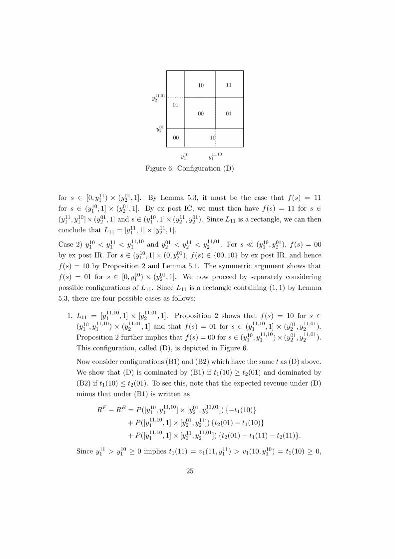
Figure 6: Configuration (D)
for s ∈ [0, y111 ) × (y01
2 , 1]. By Lemma 5.3, it must be the case that f(s) = 11for s ∈ (y10
1 , 1] × (y012 , 1]. By ex post IC, we must then have f(s) = 11 for s ∈
(y111 , y10
1 ]× (y012 , 1] and s ∈ (y10
1 , 1]× (y112 , y01
2 ). Since L11 is a rectangle, we can thenconclude that L11 = [y11
1 , 1] × [y112 , 1].
Case 2) y101 < y11
1 < y11,101 and y01
2 < y112 < y11,01
2 . For s � (y101 , y01
2 ), f(s) = 00by ex post IR. For s ∈ (y10
1 , 1] × (0, y012 ), f(s) ∈ {00, 10} by ex post IR, and hence
f(s) = 10 by Proposition 2 and Lemma 5.1. The symmetric argument shows thatf(s) = 01 for s ∈ [0, y10
1 ) × (y012 , 1]. We now proceed by separately considering
possible configurations of L11. Since L11 is a rectangle containing (1, 1) by Lemma5.3, there are four possible cases as follows:
1. L11 = [y11,101 , 1] × [y11,01
2 , 1]. Proposition 2 shows that f(s) = 10 for s ∈(y10
1 , y11,101 ) × (y11,01
2 , 1] and that f(s) = 01 for s ∈ (y11,101 , 1] × (y01
2 , y11,012 ).
Proposition 2 further implies that f(s) = 00 for s ∈ (y101 , y11,10
1 )× (y012 , y11,01
2 ).This configuration, called (D), is depicted in Figure 6.
Now consider configurations (B1) and (B2) which have the same t as (D) above.We show that (D) is dominated by (B1) if t1(10) ≥ t2(01) and dominated by(B2) if t1(10) ≤ t2(01). To see this, note that the expected revenue under (D)minus that under (B1) is written as
RF − RB = P ([y101 , y11,10
1 ] × [y012 , y11,01
2 ]) {−t1(10)}+ P ([y11,10
1 , 1] × [y012 , y11
2 ]) {t2(01) − t1(10)}+ P ([y11,10
1 , 1] × [y112 , y11,01
2 ]) {t2(01) − t1(11) − t2(11)}.
Since y111 > y10
1 ≥ 0 implies t1(11) = v1(11, y111 ) > v1(10, y10
1 ) = t1(10) ≥ 0,
25

this difference is strictly negative if t1(10) ≥ t2(01). Likewise, the expectedrevenue under (D) minus that under (B2) is written as
RF − RC = P ([y101 , y11,10
1 ] × [y012 , y11,01
2 ]) {−t2(01)}+ P ([y10
1 , y111 ] × [y11,01
2 , 1]) {t1(10) − t2(01)}+ P ([y11
1 , y11,101 ] × [y11,01
2 , 1]) {t1(10) − t1(11) − t2(11)}.
Since y112 > y01
2 ≥ 0 implies t2(11) = v2(11, y112 ) > v2(01, y01
2 ) = t2(01) ≥ 0, thedifference is strictly negative if t2(01) ≤ t1(10). Hence, (D) is never optimal.
2. L11 = [y11,101 , 1] × [y11
2 , 1]. By Proposition 2, f(s) = 10 for s ∈ (y101 , y11,10
1 ) ×(y11
2 , 1]. Furthermore, Lemma 5.1 shows that f(s) = 10 for s ∈ (y101 , 1] ×
(y012 , y11
2 ). This yields (B1).
3. L11 = [y111 , 1] × [y11,01
2 , 1]. A similar reasoning as above shows that f(s) = 01for (y10
1 , 1] × (y012 , 1] \ L11. This yields (B2).
4. L11 = [y111 , 1] × [y11
2 , 1]. In this case, we have two possibilities:
(a) f(s) = 10 for s ∈ (y101 , 1] × (y01
2 , y112 ) and f(s) = 00 for s ∈ (y10
1 , y111 ) ×
(y112 , 1]. This yields (C1).
(b) f(s) = 01 for s ∈ (y101 , 1] × (y01
2 , y112 ) and f(s) = 00 for s ∈ (y10
1 , y111 ) ×
(y112 , 1]. This yields (C2).
Case 3) y101 < y11
1 < y11,101 and y11
2 < y012 .
By ex post IR and Lemma 5.1, f(s) = 00 for s ∈ [0, y101 ) × [0, y01
2 ), f(s) = 01for s ∈ [0, y10
1 ) × (y012 , 1], and f(s) = 10 for s ∈ [y10
1 , 1] × [0, y112 ). By Lemma 5.3,
L11 can be either (i) [y11,101 , 1] × [y11
2 , 1] or (ii) s ∈ [y111 , 1] × [y11
2 , 1]. In case (i),it must be the case that f(s) = 10 for s ∈ (y10
1 , y11,101 ) × (y11
2 , 1]. Hence we obtainconfiguration (B1). In case (ii), f(s) = 00 for s ∈ (y10
1 , y111 )×(y11
2 , y012 ) by Proposition
2. Proposition 2 also implies that that f(s) ∈ {10, 00} for s ∈ (y101 , y11
1 ) × (y012 , 1].
However, Lemma 5.1 implies that f(s) = 10. This yields (A).
Case 4) y111 < y10
1 and y012 < y11
2 < y11,012 .
The reasoning similar to that of Case 3 above yields (A) and (B2).
26

Proof of Theorem 2 We first examine the optimality of configuration (B1),which requires y10
1 < y111 < y11,10
1 < 1. Since y11,101 is uniquely determined as a
function of y1 = (y101 , y11
1 ) in this case, we can use the pair of variables (y101 , y10,11
1 )instead of y1 to express the seller’s expected revenue.
RB(y11,101 , y10
1 , y112 , y01
2 )
= {1 − G2(y112 )} {1 − G1(y
11,101 )}
×{v1(11, y
11,101 ) − v1(10, y
11,101 ) + v1(10, y10
1 ) + v2(11, y112 )
}+
[1 − G1(y10
1 ) − {1 − G2(y112 )} {1 − G1(y
11,101 )}
]v1(10, y10
1 )
+ G1(y101 ) {1 − G2(y01
2 )} v2(01, y012 )
= {1 − G2(y112 )}
{r1(11, y
11,101 ) − r1(10, y
11,101 ) + {1 − G1(y
11,101 )} v2(11, y11
2 )}
+ r1(10, y101 ) + G1(y10
1 ) r2(01, y012 ).
Differentiation of RB with respect to y101 yields:
∂RB
∂y11,101
(y11,101 , y10
1 , y112 , y01
2 ) =∂r1
∂s1(10, y10
1 ) + g1(y101 ) r2(01, y01
2 ).
If y101 < z10
1 , then ∂r1∂s1
(10, y101 ) > 0 by Assumption 3 and hence the above partial
derivative is strictly positive. It follows that the optimal y101 must satisfy y10
1 ≥ z101 .
Next, differentiation of RB with respect to y11,101 yields:
∂RB
∂y11,101
(y11,101 , y10
1 , y112 , y01
2 )
= {1 − G2(y112 )}
{∂r1
∂s1(11, y11,10
1 ) − ∂r1
∂s1(10, y11,10
1 ) − g1(y11,101 ) v2(11, y11
2 )}
.
Since y11,101 > y10
1 ≥ z101 , ∂r1
∂s1(11, y11,10
1 ) < ∂r1∂s1
(10, y11,101 ) by Assumption 3. It follows
that∂RB
∂y11,101
(y11,101 , y10
1 , y112 , y01
2 ) < 0 for y11,101 > y10
1 ,
suggesting that (B1) cannot be optimal. The symmetric discussion shows that (B2)is also suboptimal. Consider next configuration (C1) which requires y10
1 < y111 < 1.
27

The expected revenue can be written as:
RD(y111 , y10
1 , y112 , y01
2 )
= {1 − G2(y112 )} {1 − G1(y11
1 )}{
v1(11, y111 ) + v2(11, y11
2 )}
+ {1 − G1(y101 )}G2(y11
2 ) v1(10, y101 )
+ G1(y101 ) {1 − G2(y01
2 )} v2(01, y012 )
= {1 − G2(y112 )} r1(11, y11
1 ) + {1 − G1(y111 )} r2(11, y11
2 )
+ G2(y112 ) r1(10, y10
1 ) + G1(y101 ) r2(01, y01
2 ).
(5)
Differentiation of RD with respect to y101 yields
∂RD
∂y101
(y111 , y10
1 , y112 , y01
2 ) = G2(y112 )
∂r1
∂s1(10, y10
1 ).
Hence, the optimal y101 should equal z10
1 . Differentiation of RD with respect to y111
on the other hand yields
∂RD
∂y111
(y111 , y10
1 , y112 , y01
2 ) = {1 − G2(y112 )} ∂r1
∂s1(11, y11
1 ) − g1(y111 ) r2(11, y11
2 ).
Since y111 > y10
1 = z101 , ∂r1
∂s1(11, y11
1 ) < ∂r1∂s1
(10, y111 ) < 0 by Assumption 3. Therefore,
the derivative is strictly negative and (C1) cannot be optimal. That (C2) cannot beoptimal is shown by a symmetric argument. We are then left with configurations in(A), which require either y11
1 ≤ yb or y112 ≤ y01
2 . The expected revenue under eachone of (A) has the same expression as that under (B2) in (5). It then follows fromthe discussion there that the optimal values satisfy y10
1 = z101 , y01
2 = z012 , y11
1 ≤ z101
and y112 ≤ z10
2 . The optimal scheme is hence (A0), which is regular.
Formula for rK(yK): We can verify that the seller’s expected revenue from theseprice offers equals
rK(yK)
= max{0, G(min {yk1k2 , . . . , yk1km}) − G(yk1)
}vk1(yk1)
+m−1∑n=2
max{0, G(min {yknkn+1, . . . , yknkm})
− G(max {ykn , yk1kn , . . . , ykn−1kn})}
vkn(ykn)
+ max{0, 1 − G(max {ykm , yk1km , . . . , ykm−1km})
}vkm(ykm).
28

When yk�kn < ykmkn for every < m and n, we can express rK(yK) as
rK(yK) =m∑
n=2
{rkn(ykn−1kn) − rkn−1(ykn−1kn)} + rk1(yk1). (6)
Proof of Lemma 4 (i) For m < n, (vn)′(·)vn(·) ≤ (vm)′(·)
vm(·) .
This readily follows from Assumption 4(iv), which implies that(
vn(s)vm(s)
)′ ≤ 0when m < n.
(ii) For each n ∈ I, rn is strictly log-concave with the (unique) maximizer zn whichsatisfies 1 > z1 ≥ · · · ≥ zI > 0.
Note that
(rn)′(s) = −g(s) vn(s) + {1 − G(s)} (vn)′(s)
= {1 − G(s)} vn(s){− g(s)
1 − G(s)+
(vn)′(s)vn(s)
}
= rn(s){− g(s)
1 − G(s)+
(vn)′(s)vn(s)
}.
Since g(s)1−G(s) is strictly increasing and (vn)′(s)
vn(s) is strictly decreasing, (rn)′(·)rn(·) is strictly
decreasing, implying that rn is strictly log-concave. Hence, the maximizer zn of rn
is unique and satisfies zn ∈ (0, 1) as rn(0) = rn(1) = 0. For m < n, zm and zn
satisfy(vm)′(zm)vm(zm)
=g(zm)
1 − G(zm)and
(vn)′(zn)vn(zn)
=g(zn)
1 − G(zn).
If zm < zn, theng(zm)
1 − G(zm)<
g(zn)1 − G(zn)
,
and hence(vm)′(zm)vm(zm)
<(vn)′(zn)vn(zn)
,
which contradicts (i).
(iii) (rm)′(s)(vm)′(s) > (rn)′(s′)
(vn)′(s′) if m < n and s < s′.The inequality is equivalent to
{1 − G(s′)}[1 − g(s′)
1 − G(s′)vn(s′)
(vn)′(s′)
]< {1 − G(s)}
[1 − g(s)
1 − G(s)vm(s)
(vm)′(s)
].
Since s < s′, this holds if g(·)1−G(·) is (strictly) increasing, and (vn)′(s′)
vn(s′) ≤ (vm)′(s)vm(s) . By
the log-concavity of vm, the latter inequality holds if (vn)′(s′)vn(s′) ≤ (vm)′(s′)
vm(s′) , which istrue by (i).
29

(iv) If m < n, s < s′, s′′ = ϕmn(s, s′), and (rn)′(s′′) ≥ (rm)′(s′′), then rn(s′) >
rmn(s, s′).We first show that (rn)′(s) ≥ (rm)′(s) implies that (rn)′(s), (rm)′(s) ≥ 0. Note
that (rn)′(s) ≥ (rm)′(s) is equivalent to
(vn)′(s) − (vm)′(s)vn(s) − vm(s)
≥ g(s)1 − G(s)
. (7)
and that (rn)′(s) ≥ 0 is equivalent to
(vn)′(s)vn(s)
≥ g(s)1 − G(s)
. (8)
Furthermore, since (vn)′(·)vn(·) ≤ (vm)′(·)
vm(·) by (i),
(vn)′(s)vn(s)
≥ (vn)′(s) − (vm)′(s)vn(s) − vm(s)
. (9)
(8) then follows from (9) and (7). That (rm)′(s) > 0 can be obtained in a similarmanner.
Now, since (rn)′(s′′), (rm)′(s′′) ≥ 0, we have (rm)′(s) > 0 and (rn)′(s′) > 0 forany s, s′ < s′′ by the strict log-concavity of rm and rn. It hence follows from (iii)that for any such s and s′,
(vm)′(s)(vn)′(s′)
<(rm)′(s)(rn)′(s′)
. (10)
Now fix s′′ such that rn(s′′) > rm(s′′), and consider the following functions ofs ∈ [0, s′′]:
s′ = (vn)−1(vm(s) + vn(s′′) − vm(s′′)
),
ands′ = (rn)−1
(rm(s) + rn(s′′) − rm(s′′)
).
Both functions are differentiable over the domain, and the graph of the former liesabove that of the latter since both of them go through (s′′, s′′) and have a singlecrossing point because of (10), which shows that the latter has a steeper slope thanthe former at any point of intersection between the two. Hence, for any s < s′′, wehave
(vn)−1(vm(s) + vn(s′′) − vm(s′′)
)> (rn)−1
(rm(s) + rn(s′′) − rm(s′′)
).
30

In other words, whenever vn(s′) = vm(s)+vn(s′′)−vm(s′′), rn(s′) > rm(s)+rn(s′′)−rm(s′′). Equivalently, we have rn(s′) > rm(s)+rn(s′′)−rm(s′′) when s′′ = ϕmn(s, s′),and s < s′. The desired conclusion then follows since by (6),
rmn(s, s′) = rn(s′′) − rm(s′′) + rm(s).
Proof of Proposition 3 Since the density g is continuous and strictly positiveover [0, 1], we have
G(ym) − G(yn)ym − yn
≥ β g(yn),
where β = min g(si)max g(si)
> 0. Hence, Assumption 5.1 holds if
β(ym − yn)(rn)′(yn)rn(yn)
> 1.
Since rm(ym) ≥ rn(yn) and ym > yn imply vm(ym) > vn(yn), using the linearity ofthe value functions, we see that the above inequality holds if
β
(ρn
ρm− 1
)yn (rn)′(yn)
rn(yn)> 1.
Substituting
(rn)′(yn)rn(yn)
=(vn)′(yn)vn(yn)
− g(yn)1 − G(yn)
=1yn
− g(yn)1 − G(yn)
into the above, we obtain
β
(ρn
ρm− 1
)(1 − yn g(yn)
1 − G(yn)
)> 1.
Since yn < ρm
ρn < ε, the increasing hazard rate condition then implies that the aboveholds if
β
(1ε− 1
)(1 − ε
g(ε)1 − G(ε)
)> 1,
which is true for a small ε > 0.For Assumption 5.2, the assumed linearity of vn implies that μn = μn = ρn−1
ρn <
ε. The inequality then holds if
ε <1 + (n − 2)εn−2
n − 1,
which is true for a small ε > 0.
31

Proof of Theorem 3 The proof of the theorem begins with Lemmas 6, 7 and 8.
Lemma 6 If z ∈ argmaxy∈[0,1]I w(y), then there exists a permutation π1, . . . , πI of1, . . . , I such that for each n = 1, . . . , I,
rπn(zπn) = max∅�=L⊂Πn
rL(zL),
where ΠI = N and Πn = N \ {πn+1, . . . , πI}. In particular, rπI (zπI ) ≥ · · · ≥rπ1(zπ1).
Proof.Step 1. rπI (zπI ) = max∅�=J⊂I rJ(zJ) for some πI ∈ I.
Suppose to the contrary that there exists K such that K ⊂ I, |K| ≥ 2, and
rK(zK) = max∅�=J⊂I
rJ(zJ). (11)
If there exists more than one such set that satisfies (11), choose any one with thesmallest cardinality |K|. Write K = {κ1, . . . , κn} for some 2 ≤ n ≤ I and κ1 <
· · · < κn. Now consider y such that
0 < yκ1 < · · · < yκn < 1, and yκn−1 < yκn < yκn−1κn < 1. (12)
Given that K has the smallest cardinality, z must satisfy (12): Otherwise, there isredundancy in K and we can find a strictly smaller set K ⊂ K such that rK(zK) =rK(zK). Write yκ1κ2, . . . , yκn−1κn as functions of yκ1 , . . . , yκn as follows:
yκ1κ2 = yκ1κ2(yκ1 , yκ2), . . . , yκn−1κn = yκn−1κn(yκn−1 , yκn).
Letzκ1κ2 = yκ1κ2(zκ1 , zκ2), . . . , zκn−1κn = yκn−1κn(zκn−1 , zκn).
z1 = ϕκ1κ2(zκ1 , zκ2), . . . , ζn−1 = ϕκn−1κn(zκn−1 , zκn).
By our choice of K, we must have 0 < ζ1 < ζ2 < · · · < ζn−1 < 1, zκ1 < zκ2 < ζ1,zκ2 < zκ3 < ζ2,. . . ,zκn−1 < zκn < ζn−1.
Now define w by
w(y) =∑
1∈J⊂Nκn /∈J
QJ(y) max∅�=L⊂J
rL(yL) + rK(yK)∑
1∈J⊂NK⊂J
QJ(y).
32

Note that LJ(z) = ∅ for any J ⊂ N such that K ⊂ J and κn ∈ J : Suppose tothe contrary that s−i ∈ LJ(z) for such a J . Since K ⊂ J , there exists k ∈ K
such that λk−1 < zk. However, since λκn−1 ≤ λk−1 < zk ≤ zκn for any such s−i,we must have λκn−1 < zκn , contradicting the assumption that κn ∈ J . Hence,∑
1∈J⊂Nκn∈J,K �⊂J
QJ(z) = 0 so that
w(z) =∑
1∈J⊂NK �⊂J
QJ(z) max∅�=L⊂J
rL(zL) + rK(zK)∑
1∈J⊂NK⊂J
QJ(z).
This suggests that w(y) ≤ w(y) for any y, and w(z) = w(z) by our hypothesis.From the definition of w, we have
∂w
∂yκn(z) =
∑1∈J⊂Nκn /∈J
∂QJ
∂yκn(z) max
∅�=L⊂JrL(zL)
+ rK(zK)∑
1∈J⊂NK⊂J
∂QJ
∂yκn(z) +
∂rK
∂yκn(zK)
∑1∈J⊂N
K⊂J
QJ(z).
Using ∑1∈J⊂Nκn /∈J
∂QJ
∂yκn(z) = −
∑1∈J⊂N
K⊂J
∂QJ
∂yκn(z),
we observe that the FOC ∂w∂yκn (z) = 0 is given by
∑1∈J⊂Nκn /∈J
∂QJ
∂yκn(zJ )
{max
∅�=L⊂JrL(zL) − rK(zK)
}+
∂rK
∂yκn(zK)
∑1∈J⊂N
K⊂J
QJ(z) = 0.
Note that the bracketed term is negative and that∑
1∈J⊂NK⊂J
QJ(z) > 0 since zκ1 <
· · · < zκn < 1. It follows that this equation holds only if
∂rK
∂yκn(zK) ≥ 0.
Recall from (6) that
rK(zK) = rκ1(zκ1) +n∑
�=2
{rκ�(zκ�−1κ�) − rκ�−1(zκ�−1κ�)
}.
The derivative of rK is hence given by
∂rK
∂yκn(zK) =
{(rκn)′(zκn−1κn) − (rκn−1)′(zκn−1κn)
} ∂yκn−1κn
∂yκn(zκn−1 , zκn).
33

Since ∂yκn−1κn
∂yκn (zκn−1 , zκn) > 0, (rκn)′(zκn−1κn) − (rκn−1)′(zκn−1κn) ≥ 0. Sincezκ�−1 < zκ� < zκ�−1κ� ≤ zκn−1κn for each ≤ n, we have by Lemma 4
rκ�(zκ�) > rκ�−1κ�(zκ�−1 , zκ�) = rκ�−1(zκ�−1) + rκ�(zκ�−1κ�) − rκ�−1(zκ�−1κ�).
Substituting this into (6), we obtain
rK(zK)
= rκ1(zκ1) +n∑
�=2
{rκ�(zκ�−1κ�) − rκ�−1(zκ�−1κ�)
}
< rκ1(zκ1) +n∑
�=2
{rκ�(zκ�) − rκ�−1(zκ�−1)
}= rκn(zκn).
This however contradicts our original supposition.
Step 2.As an induction hypothesis, suppose that for m = μ + 1, . . . , I, there exists
πm ∈ Πm such thatrπm(zπm) = max
∅�=L⊂Πm
rL(zL).
We will show thatrK(zK) < max
∅�=J⊂Πμ
rJ(zJ)
for any K such that K ⊂ Πμ and |K| ≥ 2. Suppose to the contrary that rK(zK) =max∅�=J⊂Πμ
rJ(zJ ) for some K = {κ1, . . . , κn} such that K ⊂ Πμ and n ≥ 2. Define
w(y) =∑
1∈J⊂Πμκn /∈J
QJ(y) max∅�=L⊂J
rL(yL) + rK(yK)∑
1∈J⊂ΠμK⊂J
QJ(y)
+I∑
m=μ+1
rπm(yπm)∑
1∈J⊂Πmπm∈J
QJ(y).
As in Step 1, we observe that LJ(z) = ∅ for any J such that κn ∈ J and K ⊂ J .18
Then w(y) ≤ w(y) for any y and w(z) = w(z) by the induction hypothesis. Since∑1∈J⊂Πm
πm∈J
QJ(y) = P(λπm−1 ≥ yπm, max
�>m(λπ�−1 − yπ�) < 0
),
18The reasoning is the same as that following the definition of w in Step 1.
34

the third term in the definition of w is independent of yΠμ . It follows that
∂w
∂yκn(z) =
∑1∈J⊂Πμ
κn /∈J
∂QJ
∂yκn(z) max
∅�=L⊂JrL(zL) + rK(zK)
∑1∈J⊂Πμ
K⊂J
∂QJ
∂yκn(z)
+∂rK
∂yκn(zK)
∑1∈J⊂Πμ
K⊂J
QJ(z).
Noting that∑
1∈J⊂Πμκn /∈J
∂QJ
∂yκn (z) = −∑1∈J⊂Πμ
K⊂J
∂QJ
∂yκn (z), we conclude as before that
∂rK
∂yκn (zK) ≥ 0. Using the same logic as in Step 1, we can then derive the contradictionthat rK(zK) < rκn(zκn). This advances the induction step and completes the proof.
Lemma 7 If z ∈ argmaxy∈[0,1]I w(y), then z ∈ (0, 1)I .
Proof. Suppose not and take the largest n for which zπn = 0 or 1, where π1, . . . , πI
are as defined in Lemma 6. It would then follow that rπn(zπn) = 0 and hence thatrπ�(zπ�) = 0 for every < n as well. Define z to be such that
zπμ =
⎧⎨⎩zπμ if μ = n,
12 if μ = n.
We then have
w(z) ≥I∑
μ=1
rπμ(zπμ)∑
1∈J⊂Πμπμ∈J
QJ(z)
= rπn(zπn)P(λπn−1 ≥ zπn , max
�>n(λπ�−1 − zπ�) < 0
)
+I∑
μ=n+1
rπμ(zπμ)P(λπμ−1 ≥ zπμ , max
�>μ(λπ�−1 − zπ�) < 0
)
>I∑
μ=n+1
rπμ(zπμ)P(λπμ−1 ≥ zπμ , max
�>μ(λπ�−1 − zπ�) < 0
)= w(z),
where the inequality holds since rπn(12 ) > 0 and zπ� > 0 for > n. This is a
contradiction.
35
Lemma 8 Suppose that Assumptions 4 and 5 hold. If z ∈ argmaxy∈[0,1]I w(y), thenπμ = μ for μ = 1, . . . , I, or equivalently,
r1(z1) ≤ · · · ≤ rI(zI).
Proof. Note first that argmaxy w(y) = ∅ since w is a continuous function over thecompact domain [0, 1]I . Let z = (z1, . . . , zI) ∈ argmaxy w(y) be any maximizer.We prove the claim by induction over μ = 1, . . . , I.
Step 1. rI(zI) = max∅�=J⊂I rJ(zJ).Given the conclusion of Lemma 6, the claim is equivalent to πI = I, where
π1, . . . .πI are as defined there. Suppose to the contrary that πI < I, and take n < I
such that πn = I. If we define
w(y) =I∑
μ=1
rπμ(yπμ)∑
1∈J⊂Πμπμ∈J
QJ(y)
=I∑
μ=1
rπμ(yπμ)P(λπμ−1 ≥ yπμ , max
�>μ(λπ�−1 − yπ�) < 0
),
then w(y) ≤ w(y) for any y and w(z) = w(z). Differentiating w with respect toyπn = yI , we obtain
∂w
∂yπn(y) =
n−1∑μ=1
rπμ(yπμ)∑
1∈J⊂Πμπμ∈J
∂QJ
∂yπn(y)
+ (rπn)′(yπn)∑
1∈J⊂Πnπn∈J
QJ(y)
+ rπn(yπn)∑
1∈J⊂Πnπn∈J
∂QJ
∂yπn(y).
(13)
Since z ∈ (0, 1)I by Lemma 7, the FOC ∂w∂yπn (z) = 0 holds at y = z. Furthermore,
since rπμ(zπμ) ≤ rπn(zπn) for every μ < n, and
∑1∈J⊂Πμ
πμ∈J
∂QJ
∂yπn(z) = −
∑1∈J⊂Πn
πn∈J
∂QJ
∂yπn(z) > 0, (14)
36

the sum of the first and third terms on the right-hand side of (13) evaluated at z is≤ 0, implying that (rπn)′(zπn) ≥ 0. This and rπ�(zπ�) ≥ rπn(zπn) for > n togetherimply that zπ� > zπn for > n. Let zπm be the smallest among zπn+1, . . . , zπI .
For any y such that yπn < yπm < min�>n,� �=m yπ�, we now evaluate the probabil-ity
∑1∈J⊂Πn
πn∈JQJ(y) appearing in (13) in two ways. First, assigning just one of I − 1
signals to the interval [yπn , yπm ], we see that∑1∈J⊂Πn
πn∈J
QJ(y) = P(λπn−1 ≥ yπn , max
�>n(λπ�−1 − yπ�) < 0
)
=(
I − 11
){G(yπm) − G(yπn)}
× P(λπn−2
I−2 ≥ yπn , max�>n
(λπ�−1I−2 − yπ�) < 0
),
(15)
where λkI−2 is the kth largest value among I − 2 signals, and λ�
k = 0 wheneverk < . Second, suppose we assign p of I − 1 signals to [yπn , yπm] and the remainingq = I−1−p signals to (yπm, 1]. In this case, q < πm−1 must hold since λπm−1 < yπm.Hence, ∑
1∈J⊂Πnπn∈J
QJ(y) = P(λπn−1 ≥ yπn ,max
�>n(λπ�−1 − yπ�) < 0
)
=∑
p+q=I−1q<πm−1
(I − 1
p
){G(yπm) − G(yπn)}p
× P(
max�>n,� �=m
(λπ�−1q − yπ�) < 0, λq
q ≥ yπm
).
(16)
Differentiating (16) with respect to yπn = yI and rearranging, we obtain∑1∈J⊂Πn
πn∈J
∂QJ
∂yπn(y)
= −(I − 1) g(yπn)P(λπn−2
I−2 ≥ yπn , max�>n
(λπ�−1I−2 − yπ�) < 0
).
(17)
Now substitute (15) and (17) into (13) and set y = z to get
∂w
∂yπn(z)
≥ P(λπn−2
I−2 ≥ zπn , max�>n
(λπ�−1I−2 − zπ�) < 0
)× (I − 1)
[−g(zπn) rπn(zπn) + (rπn)′(zπn) {G(zπm) − G(zπn)}
]> 0.
37

where the first inequality follows from the fact that the first term on the right-hand side of (13) is positive (i.e., (14)), and the second from Assumption 1 alongwith the fact that zπn < zπm and rπm(zπm) ≥ rπn(zπn). We have hence derived acontradiction to the fact that z is an interior maximizer.
Step 2. For n = 1, . . . , I − 1, rn(zn) = max�≤n r�(z�).As an induction hypothesis, suppose that the statement holds for n + 1, . . . , I.
Define
wn(y) =n∑
k=1
rπk(yπk)∑
1∈J⊂Πkπk∈J
QJ(y) +I∑
k=n+1
rk(yk)∑
1∈J⊂Nmax J=k
QJ(y)
=n∑
k=1
rπk(yπk)∑
1∈J⊂Πkπk∈J
QJ(y)
+I∑
k=n+1
P(λk−1 ≥ yk, max
�>k(λ�−1 − y�) < 0
)rk(yk).
We then have wn(y) ≤ w(y) for any y, and by the induction hypothesis, wn(z) =w(z). Hence, since z is a maximizer of w, it is a maximizer of wn as well. Notethat the second term on the right-hand side above is independent of (y1, . . . , yn),and the first term has the same form as w in Step 1 with the only exception that n
replacing I. This implies that the same reasoning as that in step 1 proves
rn(zn) = max�≤n
r�(z�).
We now return to the proof of the theorem. We will show that any maximizer z
of w : RI → R satisfies zI ≤ · · · ≤ z1 under Assumption 5.2. For n = 1, . . . , I andy ∈ [0, 1]I , define
Rn(y) =∑
1∈J⊂Inn∈J
QJ(y) = P (λn−1 ≥ yn, max�>n
(λ�−1 − y�) < 0).
For any y such that yI > yI−1, we have
∂R1
∂yI(·) = · · · =
∂RI−2
∂yI(·) = 0.
Furthermore, sinceRI(y) = {1 − G(yI)}I−1,
38

and
RI−1(y)
= P (λI−2 ≥ yI−1, λI−1 < yI)
= (I − 1){1 − G(yI−1)}I−2G(yI−1)
+ {1 − G(yI−1)}I−1 − {1 − G(yI)}I−1,
we have∂RI
∂yI(y) = −(I − 1){1 − G(yI)}I−2g(yI),
and∂RI−1
∂yI−1(y) = −(I − 1)(I − 2){1 − G(yI−1)}I−3G(yI−1)g(yI−1).
Suppose now that there exists a maximizer z of w such that zI > zI−1. Sincez ∈ (0, 1)I by Lemma 7, z satisfies the FOC’s:
∂w
∂yI(z) =
∂RI−1
∂yI(z) rI−1(zI−1)
+∂RI
∂yI(z) rI(zI) + RI(z) (rI)′(zI) = 0,
and
∂w
∂yI−1(z) =
I−1∑n=1
∂Rn
∂yI−1(z) rn(zn)
+ RI−1(z) (rI−1)′(zI−1) = 0.
Noting that ∂RI−1
∂yI (z) = −∂RI−1
∂yI (z) > 0, and∑I−2
n=1∂Rn
∂yI−1 (z) = −∂RI−1
∂yI−1 (z) > 0, weobtain
(rI)′(zI)rI(zI)
= − 1RI(z)
∂RI
∂yI(z)
{1 − rI−1(zI−1)
rI(zI)
},
= (I − 1)g(zI)
1 − G(zI )
{1 − rI−1(zI−1)
rI(zI)
},
(18)
and
(rI−1)′(zI−1)rI−1(zI−1)
=1
RI−1(z)
{−∂RI−1
∂yI−1(z) −
I−2∑n=1
∂Rn
∂yI−1(z)
rn(zn)rI−1(zI−1)
}
≤ − 1RI−1(z)
∂RI−1
∂yI−1(z)
{1 − r1(z1)
rI−1(zI−1)
}.
(19)
39

Let RI−1(y) = RI−1(y), where yk = yk for k = I and yI = yI−1. Then RI−1(y) ≤RI−1(y), and
− 1RI−1(z)
∂RI−1
∂yI−1(z) = (I − 2)
g(zI−1)1 − G(zI−1)
.
Since zI−1 < z1 = z1 and (r1)′(y1) > 0 for y1 < z1, we have
r1(z1)rI−1(zI−1)
>r1(zI−1)
rI−1(zI−1)=
v1(zI−1)vI−1(zI−1)
≥I−1∏k=2
μk.
Hence, (19) implies
(rI−1)′(zI−1)rI−1(zI−1)
≤ (I − 2)g(zI−1)
1 − G(zI−1)
{1 −
I−1∏k=2
μk
}. (20)
Since (rI)′(zI) > 0, zI−1 < zI and (rI−1)′(y) > 0 whenever (rI)′(y) > 0, we alsohave
rI−1(zI−1)rI(zI)
<rI−1(zI)rI(zI)
=vI−1(zI)vI(zI)
≤ μI .
substituting this into (18), we get
(rI)′(zI)rI(zI)
> (I − 1)g(zI)
1 − G(zI)(1 − μI). (21)
Combining (20) and (21) together, we see that
(I − 1)g(zI)
1 − G(zI)(1 − μI)
<(rI)′(zI)rI(zI)
≤ (rI)′(zI−1)rI(zI−1)
≤ (rI−1)′(zI−1)rI−1(zI−1)
≤ (I − 2)g(zI−1)
1 − G(zI−1)
{1 −
I−1∏k=2
μk
},
where the inequalities in the second line hold because (rI)′rI is decreasing, zI > zI−1.
and (rI)′(si)rI(si)
≤ (rI−1)′(si)rI−1(si)
for any si. Furthermore, given the increasing hazard rate,we must have
(I − 1) (1 − μI) < (I − 2)
{1 −
I−1∏k=2
μk
}.
This, however, contradicts Assumption 5.2.
40

As an induction hypothesis, suppose that zI ≤ · · · ≤ zn. Suppose that zn >
zn−1. For any y such that yI ≤ · · · ≤ yn and yn > yn−1, we have ∂R1
∂yn (y) = · · · =∂Rn−1
∂yn (y) = 0, and
Rn(y)
= P (λn−1 ≥ yn, λn < yn+1, . . . , λI−1 < yI)
=(
I − 1n − 1
){1 − G(yn)}n−1 P (λ1
I−n < yn+1, . . . , λI−nI−n < yI),
where λkI−n is the kth largest value among I − n signals. Hence,
∂Rn
∂yn(y)
= −g(yn)(n − 1) {1 − G(yn)}n−2
(I − 1n − 1
)P (λ1
I−n < yn+1, . . . , λI−nI−n < yI),
and1
Qn(y)∂Qn
∂yn(y) = −(n − 1)
g(yn)1 − G(yn)
.
The first-order condition ∂w∂yn (z) = 0 then yields
(rn)′(zn)rn(zn)
= − 1Qn
∂Qn
∂yn
{1 − rn−1(zn−1)
rn(zn)
}
= (n − 1)g(zn)
1 − G(zn)
{1 − rn−1(zn−1)
rn(zn)
}.
(22)
On the other hand, suppose yn+1 ≤ yn−1 < yn. Other cases can be treated in asimilar manner.
Rn−1(y)
= P (λn−2 ≥ yn−1, λn−1 < yn, λn < yn+1, . . . , λI−1 < yI)
=(
I − 1n − 2
){1 − G(yn−1)}n−2
×[(I − n + 1){G(yn−1) − G(yn+1)}P (λ1
I−n < yn+1, . . . , λI−nI−n < yI)
+ P (λ1I−n+1 < yn+1, . . . , λI−n+1
I−n+1 < yI)]
+(
I − 1n − 1
)[{1 − G(yn−1)}n−1 − {1 − G(yn)}n−1
]P (λ1
I−n < yn+1, . . . , λI−nI−n < yI).
41

Differentiating Rn−1 with respect to yn−1, we obtain
∂Rn−1
∂yn−1(y)
= −g(yn−1)(
I − 1n − 2
)(n − 2){1 − G(yn−1)}n−3
×[(I − n + 1){G(yn−1) − G(yn+1)}P (λ1
I−n < yn+1, . . . , λI−nI−n < yI)
+ P (λ1I−n+1 < yn+1, . . . , λI−n+1
I−n+1 < yI)].
Let Rn−1(y) = Rn−1(y), where yk = yk for k = n and yn = yn−1. We haveRn−1(y) ≤ Rn−1(y) and can also verify that
1Rn−1(y)
∂Rn−1
∂yn−1(y) = −(n − 2)
g(yn−1)1 − G(yn−1)
.
The first-order condition ∂w∂yn−1 (z) = 0 then yields
(rn−1)′(zn−1)rn−1(zn−1)
= − 1Rn−1(z)
[n−1∑k=1
∂Rk
∂yn−1(z)
rk(zk)rn−1(zn−1)
]
≤ (n − 2)g(yn)
1 − G(yn)
(1 − r1(z1)
rn−1(zn−1)
)
< (n − 2)g(yn)
1 − G(yn)
(1 − r1(zn−1)
rn−1(zn−1)
)
≤ (n − 2)g(yn)
1 − G(yn)
(1 −
n−1∏k=2
μk
).
(23)
On the other hand,
(rn)′(zn)rn(zn)
= (n − 1)g(zn)
1 − G(zn)
{1 − rn−1(zn−1)
rn(zn)
}
> (n − 1)g(zn)
1 − G(zn)
{1 − rn−1(zn)
rn(zn)
}
> (n − 1)g(zn)
1 − G(zn){1 − μn} .
(24)
Just as in Step 1, we can combine (23) and (24) to yield a contradiction to Assump-tion 5.2, which is equivalent to
(n − 1) {1 − μn} ≥ (n − 2)
(1 −
n−1∏k=2
μk
).
42

This advances the induction step and completes the proof.
Proof of Lemma 1 Take any m ∈ M(y). Let n be such that n > m and ym < yn.Take s such that ym < s1 = · · · = sn < yn and sn+1 = · · · = sI = 0. Symmetryand ex post IR then imply that f(s) equals either (0, . . . , 0︸ ︷︷ ︸
n
, 1, . . . , 1︸ ︷︷ ︸I−n
), (0, . . . , 0), or
(1, . . . , 1). When f(s) = (0, . . . , 0, 1, . . . , 1), tI−n = 0 should hold by ex post IR, andwhen f(s) = (1, . . . , 1), then tI = 0 should hold by ex post IR. Suppose now thatm ∈ K(f), or that there exists s such that |f(s)| = m. By symmetry, we can takes such that f(s) = (1, . . . , 1︸ ︷︷ ︸
m
, 0, . . . , 0).
If f(s) = (0, . . . , 0). then s is a profitable deviation for the coalition J = I at s:For i = 1, . . . ,m,
vi(f(s), si) − ti(f(s)) = vm(si) − tm > 0 = vi(f(s), si) − ti(s),
where the inequality follows from the fact that si > ym. Furthermore, for i =m + 1, . . . , I,
vi(f(s), si) − ti(f(s)) = 0 = vi(f(s), si) − ti(s).
If f(s) = (0, . . . , 0︸ ︷︷ ︸n
, 1, . . . , 1), then tI−n = 0 as noted above and s is a profitable
deviation for the coalition J = I at s: For i = 1, . . . ,m,
vi(f(s), si) − ti(f(s)) = vm(si) − tm > 0 = vi(f(s), si) − ti(f(s)),
for i = m + 1, . . . , n,
vi(f(s), si) − ti(f(s)) = 0 = vi(f(s), si) − ti(f(s)),
and for i = n + 1, . . . , I,
vi(f(s), si) − ti(f(s)) = 0 = vI−n(0) − tI−n = vi(f(s), si) − ti(f(s)).
If f(s) = (1, . . . , 1), then yI = 0 as noted above and s is a profitable deviation forthe coalition J = I at s: For i = 1, . . . ,m,
vi(f(s), si) − ti(f(s)) = vI(si) − tI > vm(si) − tm = vi(f(s), si) − ti(f(s)),
and for i = m + 1, . . . , I,
vi(f(s), si) − ti(f(s)) = vI(si) − tI > 0 = vi(f(s), si) − ti(f(s)).
Therefore, (f, t) is not coalitionally strategy-proof.
43

Proof of Lemma 2 For K and y such that K ∩ M(y) = ∅, w can alternativelybe written as
w(K, y) =∑k∈K
P (λk−1 ≥ yk,max�∈K�>k
(λ�−1 − y�) < 0) rk(yk).
Let (f, y) be such that K(f) = K. Fix k ∈ K and s−i such that λk−1 ≥ yk andmax �∈K
�>k(λ�−1 − y�) < 0. By our choice of s−i, |f(si, s−i)| ≤ k for any si by ex post
IR. Moreover, if si < yk, then si < ym for any m < k so that |fi(si, s−i)| = 0. Inwhat follows, we show that |f(si, s−i)| = k whenever si > yk. If this holds, then
Esi [ti(f(si, s−i)) | s−i] = P (si < yk)Esi [ti(f(si, s−i)) | si < yk, s−i]
+ P (si > yk)Esi [ti(f(si, s−i)) | si > yk, s−i]
= P (si > yk) tk
= rk(yk).
This in turn implies that
R(f, t) = Es[ti(f(s))]
= Es−i [Esi [ti(f(si, s−i)) | s−i]]
=∑k∈K
rk(yk)P (λk−1 ≥ yk, max�∈K�>k
(λ�−1 − y�) < 0)
= w(K, y).
Suppose that si > yk and denote s = (si, s−i). We will derive a contradiction whenm = |f(s)| < k. Let J ⊂ I be such that i ∈ J , |J | = k, and
{j : fj(s) = 1} ⊂ J ⊂ {j : sj ≥ yk}.Such a set J exists since fj(s) = 1 implies that sj ≥ ym ≥ yk by ex post IR. Sincek ∈ K = K(f), take s such that |f(s)| = k and {j : fj(s) = 1} = J . Such a signalprofile s exists by symmetry. When sj ≥ yk, note that
vk(sj) − vm(sj) ≥ vk(yk) − vm(yk) ≥ vk(yk) − vm(ym),
where the first inequality follows from (vk)′ > (vm)′, and the second from yk ≤ ym.We will show that s is a profitable deviation for I at s:For j ∈ J ∩ {j : fj(s) = 1},
vj(f(s), sj) − tj(f(s)) = vk(sj) − vk(yk)
≥ vm(sj) − vm(ym)
= vj(f(s), sj) − tj(f(s)).
(25)
44

For j ∈ J ∩ {j : fj(s) = 0},
vj(f(s), sj) − tj(f(s)) = vk(sj) − tk ≥ 0 = vj(f(s), sj) − tj(f(s)). (26)
For j ∈ I \ J ,
vj(f(s), sj) − tj(f(s)) = 0 = vj(f(s), sj) − tj(f(s)).
Since si > yk, if fi(s) = 1, then (25) holds with strict inequality for j = i, andif fi(s) = 0, then (26) holds with strict inequality for j = i. Hence, (f, t) is notstrategy-proof.
Proof of Lemma 4 Take any J ⊂ I, s = (sJ , s−J) and sJ . Denote s = (sJ , s−J)and k = |f(s)|. If |f(s)| = m > k, then |{i : si ≥ zk}| = k < m and |{i : si ≥zm}| = m by the definition of a regular scheme. Hence, there exists at least onebuyer i ∈ J for whom si < zm, si ≥ zm and fi(s) = 1. It follows that for this i,
vi(f(s), si) − ti(f(s)) = vm(si) − tm < 0 ≤ vi(f(s), si) − ti(f(s)),
suggesting that sJ is not a profitable deviation of J at s. If |f(s)| = m < k, take anyi ∈ J for whom fi(s) = 1. If there exists no such j ∈ J , then s is not a profitabledeviation for J . Since zm ≥ zk, we have vk(zm) − vm(zm) ≥ vk(zk) − vm(zm).Furthermore, since (vk)′ ≥ (vm)′, vk(si)−vm(si) ≥ vk(zm)−vm(zm) for any si ≥ zm.It follows that vk(si) − vm(si) ≥ vk(zk) − vm(zm) for any si ≥ zm. In other words,if fi(s) = 1 and si ≥ zm, then
vi(f(s), si) − ti(f(s)) = vm(si) − tm
= vm(si) − vm(zm)
≤ vk(si) − vk(zk)
= vi(f(s), si) − ti(f(s)).
This implies that s is not a profitable deviation for J at s.
Proof of Theorem 4 We will show that when K = N and y ∈ [0, 1]I , w(K, y) ≤w(I, y) for some y such that yI ≤ · · · ≤ y1. Since w(N, ·) is continuous over thecompact set {y : yI ≤ · · · ≤ y1}, it achieves a maximum at some z in this set.Hence, w(N, z) = maxK⊂N, y∈[0,1]I w(K, y), and by Proposition 4, there exists aregular scheme (f, t) such that R(f, t) = w(N, z).
45

When yk = 1 for some k ∈ K, then w(K, y) = w(K \ {k}, y) so that we mayrestrict attention to the case where maxk∈K yk < 1. Suppose that K = N and fixany y such that K ∩ M(y) = ∅. We have
w(K, y) =∑�∈K
P (λ�−1 ≥ y�, maxm∈Km>�
(λm−1 − ym) < 0) r�(y�).
Let n = min N \ K and K = K ∪ {n}. If n = 1, then let y be such that y1 =maxk∈K yk and yk = yk for k > 1. Then K ∩ M(y) = ∅ and w(K, y) is given by
w(K, y) =∑k∈K
P (λk−1 ≥ yk, max�∈K�>k
(λ�−1 − y�) < 0) rk(yk)
= P (max�∈K
(λ�−1 − y�) < 0) r1(y1)
+∑k∈K
P (λk−1 ≥ yk, max�∈K�>k
(λ�−1 − y�) < 0) rk(yk)
≥ w(K, y).
If n > 1, then n − 1 ∈ K and let y be such that
yk =
⎧⎨⎩yk if k = n,
yn−1 if k = n.
Since K ∩ M(y) = ∅, w is given by
w(K, y) =∑�∈K
P(λ�−1 ≥ y�, max
m∈Km>�
(λm−1 − ym) < 0)
r�(y�)
=∑�∈K�<n
P(λ�−1 ≥ y�, λn−1 < yn−1, max
m∈Km>�
(λm−1 − ym) < 0)
r�(y�)
+ P(λn−1 ≥ yn−1, max
m∈Km>n
(λm−1 − ym) < 0)
rn(yn−1)
+∑�∈K�>n
P(λ�−1 ≥ y�, max
m∈Km>�
(λm−1 − ym) < 0)
r�(y�).
46
Noting that λn−2 < yn−1 implies λn−1 < yn−1, we can reduce the above to
w(K, y) =∑�∈K
�<n−1
P(λ�−1 ≥ y�, max
m∈Km>�
(λm−1 − ym) < 0)
r�(y�)
+ P(λn−2 ≥ yn−1, λn−1 < yn−1, max
m∈Km>n−1
(λm−1 − ym) < 0)
rn−1(yn−1)
+ P(λn−1 ≥ yn−1, max
m∈Km>n
(λm−1 − ym) < 0)
rn(yn−1)
+∑�∈K�>n
P(λ�−1 ≥ y�, max
m∈Km>�
(λm−1 − ym) < 0)
r�(y�).
Using rn(yn−1) ≥ rn−1(yn−1), and
P(λn−2 ≥ yn−1, λn−1 < yn−1, max
m∈Km>n−1
(λm−1 − ym) < 0)
+ P(λn−1 ≥ yn−1, max
m∈Km>n
(λm−1 − ym) < 0)
= P(λn−2 ≥ yn−1, max
m∈Km>n−1
(λm−1 − ym) < 0),
we obtain w(K, y) ≥ w(K, y). Iteration of this process shows that w(I, y) ≥ w(K, y)for some y.
References
[1] Parimal Kanti Bag, and Eyal Winter (1999), “Simple Subscription Mechanismsfor Excludable Public Goods,” Journal of Economic Theory 87, 72-94.
[2] Luis M. B. Cabral, David J. Salant, and Glenn A. Woroch (1999), “Monopolypricing with network externalities,” International Journal of Industrial Organi-zation, 17, 199-214.
[3] Rajat Deb, and Laura Razzolini (1999a), “Voluntary cost sharing for an ex-cludable public project,” Mathematical Social Science, 37, 123-138.
[4] Rajat Deb, and Laura Razzolini (1999b), “Auction-like mechanisms for pricingexcludable public goods,” Journal of Economic Theory, 88, 340-368.
[5] Philip H. Dybvig, and Chester S. Spatt (1983),“ Adoption externalities aspublic goods,”Journal of Public Economics, 20, 231-247.
47

[6] Douglas Gale (1995),“Dynamic coordination games,”Economic Theory, 5, 1-18.
[7] Douglas Gale (2001), “Monotone games with positive spillovers,” Games andEconomic Behavior, 37, 295-320.
[8] Michael L. Katz, and Carl Shapiro (1985), “Network externalities, competition,and compatibility,” American Economic Review, 75, 424-440.
[9] Michael L. Katz, and Carl Shapiro (1986), “Technology adoption in the presenceof network externalities,” Journal of Political Economy, 94, 822-841.
[10] Herve Moulin (1994), “Serial cost sharing of excludable public goods,” Reviewof Economic Studies, 61, 305-325.
[11] Jack Ochs, and In-Uck Park (2009), “Overcoming the coordination problem:dynamic formation of networks,” working paper.
[12] In-Uck Park (2004), “A simple inducement scheme to overcome adoption ex-ternalities,” Contributions to Theoretical Economics, 4(1), Article 3.
[13] Jeffrey H. Rohlfs (1974), “A theory of interdependent demand for a communi-cations service,” Bell Journal of Economics 5 (1), 16-37.
[14] Tadashi Sekiguchi (2009), “Pricing of durable network goods under dynamiccoordination failure,” working paper.
[15] Tatsuhiro Shichijo, and Yuji Nakayama (2009) “A two-step subsidy schemeto overcome network externalities in a dynamic game,” The B.E. Journal ofTheoretical Economics, 9(1) (Topics), Article 4.
[16] Arun Sundararajan (2007)“Local network effects and complex network struc-ture,”The B.E. Journal of Theoretical Economics, 7(1) (Contributions), Article46.
48