Monitoring Vegetation on Railway Embankments - ICOET

Proceedings of the 2013 International Conference on Ecology and Transportation (ICOET 2013)

Monitoring Vegetation on Railway Embankments:

Supporting Maintenance Decisions

Roger G. Nyberg (+46 23 778873, [email protected]), M.Sc.,

School of Engineering and the Built Environment, Edinburgh Napier University, EH10

5DT Edinburgh, UK, and Department of Computer Engineering, Dalarna University,

78170 Borlange, Sweden

Narendra K. Gupta, Professor,

School of Engineering and the Built Environment, Edinburgh Napier University, EH10

5DT Edinburgh, UK

Siril Yella, Ph.D.,

Department of Computer Engineering, Dalarna University, 78170 Borlange, Sweden

Mark Dougherty, Professor,

Department of Computer Engineering, Dalarna University, 78170 Borlange, Sweden

Abstract The national railway administrations in Scandinavia, Germany, and Austria mainly resort to manual

inspections to control vegetation growth along railway embankments. Manually inspecting railways is slow

and time consuming. A more worrying aspect concerns the fact that human observers are often unable to

estimate the true cover of vegetation on railway embankments. Further human observers often tend to

disagree with each other when more than one observer is engaged for inspection. Lack of proper techniques

to identify the true cover of vegetation even result in the excess usage of herbicides; seriously harming the

environment and threating the ecology. Hence work in this study has investigated aspects relevant to human

variation and agreement to be able to report better inspection routines. This was studied by mainly carrying

out two separate yet relevant investigations.

First, thirteen observers were separately asked to estimate the vegetation cover in nine images acquired (in

nadir view) over the railway tracks. All such estimates were compared relatively and an analysis of variance

resulted in a significant difference on the observers’ cover estimates (p<0.05). Bearing in difference between

the observers, a second follow-up field-study on the railway tracks was initiated and properly investigated.

Two railway segments (strata) representing different levels of vegetation were carefully selected. Five sample

plots (each covering an area of one- by-one meter) were randomized from each stratum along the rails from

the aforementioned segments and ten images were acquired in nadir view. Further three observers (with

knowledge in the railway maintenance domain) were separately asked to estimate the plant cover by visually

examining the plots. Again an analysis of variance resulted in a significant difference on the observers’ cover

estimates (p<0.05) confirming the result from the first investigation.

The differences in observations are compared against a computer vision algorithm which detects the "true"

cover of vegetation in a given image. The true cover is defined as the amount of greenish pixels in each

image as detected by the computer vision algorithm.

Results achieved through comparison strongly indicate that inconsistency is prevalent among the estimates

reported by the observers. Hence, an automated approach reporting the use of computer vision is suggested,

thus transferring the manual inspections into objective monitored inspections.

mailto:[email protected]

Nyberg, Gupta, Yella, and Dougherty 2

INTRODUCTION

Subcontracting railway maintenance activities is not trivial. The Swedish Transport

Administration (STA) invites for a competitive price quote for certain maintenance

periods, involving various activities. Maintenance subcontractors are finding it extremely

difficult to provide an estimate (often speculative) concerning vegetation control. Reliable

information about the actual vegetation status is most often not available, thus maintenance

actions are carried out by subcontractors on a periodic basis irrespective of the condition,

which wastes resources. Concerning use of herbicides it is important to substantially

reduce the amount of herbicides (used to fight vegetation) along railways for

environmental reasons.

Growing vegetation along railways is often extensive, thus maintaining an area free from

vegetation, like weeds, shrubbery, trees, is a constant struggle against nature. The main

reason for the STA to control vegetation on and along railways is safety for passengers and

their staff (Banverket, 2000), (Banverket, 2001).

The national railway administrations in Scandinavia, Germany, and Austria mainly resort

to manual inspections to control vegetation growth along railway embankments. Manually

inspecting railways is slow and time consuming. A more worrying aspect concerns the fact

that human observers are often unable to estimate the true cover of vegetation on railway

embankments. Further human observers often tend to disagree with each other when more

than one observer is engaged for inspection. Lack of proper techniques to identify the true

cover of vegetation even result in the excess usage of herbicides; seriously harming the

environment and threating the ecology.

Measuring Terrestrial Vegetation

Plant species can be described by a number of characteristics, also called vegetation

attributes. In general, the most commonly used attributes when monitoring vegetation are:

cover (vertical projection of a plant on a reference area), density (number of individuals per

area unit), frequency of occurrence (presence-absence of a species in repeatedly placed

sample plots, or points), biomass, and different measures of plant vigour (Mueller-

Dombois et al., 2003, p.67) (Elzinga et al., 1998, p.101), (Bonham, 1989).

Plant Cover

The measurable quantity (plant) cover is one of the most commonly used variables in

ecology for monitoring ground state (Bonham et al., 2005), (Mueller-Dombois et al., 2003,

p.80). Usually cover is defined as the vertical projection of vegetation from the ground as

viewed from above, i.e. nadir, or bird’s-eye view of the vegetation.

In this work cover has been used because of its common use and the relative ease of

transferring its concepts into images, and equally important: cover has a linear relationship


reflecting the actual amount of aboveground biomass concerning low open herbaceous

plants growing in low nutrient and moisture soil (Rottgermann et al., 2000). These

conditions are often similar to the environment on a railway embankment.

There are several approaches for estimating, or measuring, cover depending on the

sampling unit. In general, a sampling unit is an element (or set of elements) which is

considered for selection out of the total population. Often used primary sampling units are

individual plants, lines (transects), points, or quadrats (in this context a quadrat is a

sampling frame of any shape which not necessarily is a geometric regular quadrilateral).

Combinations can be used like for example: point-quadrats (i.e. a number of points, which

could be pins or wired cross hairs, within a plot), sub-plots (i.e. small plots, which could

composed of a grid, within a bigger plot, e.g. the sub-plot frequency method), or sample

plots or sample points along a line. The type of sampling unit is dependent on what type of

vegetation attribute is measured (Elzinga et al., 1998 p.101).

Depending on the author different types of cover goes under different names, and are also

interpreted differently. This partly depends on how cover is defined, i.e. is how and what to

measure when estimating cover. This has been studied by (Fehmi, 2010) who compared

published common plant cover definitions as well as uses of cover in research in the time

span between 1950 to 2007. In order not to limit the survey three overall definitions were

made to in an attempt to incorporate all cover definitions of the authors. The three

suggested over-all cover definitions while conducting this comparative survey were: 1)

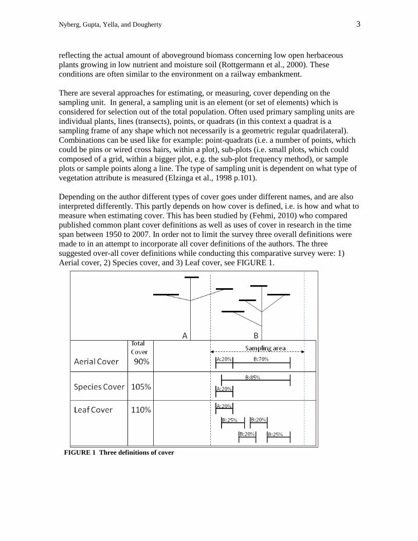
Aerial cover, 2) Species cover, and 3) Leaf cover, see FIGURE 1.

FIGURE 1 Three definitions of cover


The total cover percentage result is depending on how the observer

chooses to define cover. This is outlined in FIGURE 1, where two

plants (A and B) are seen horizontally from the side. Plant A is

partially in the sampling area and plant B is fully in the sampling

area. If the observer (who observes the sampling area vertically

from above) measures cover by making use of all the three cover

definitions the result will be threefold: 90%, 105%, and 110%,

respectively.

(Elzinga et al., 1998, p.178) describes two types of cover, see

Figure 2: 1) Basal cover defines the area where the plant inter-

sects the ground, and 2) Aerial cover is the vegetation covering the

ground surface above the ground surface. Concerning aerial cover two types can be

distinguished, namely foliar cover and canopy cover (Coulloudon et al., 1999), see

FIGURE 3.

FIGURE 3 Aerial foliar cover (left), and aerial canopy cover (right) (Coulloudon et. al, 1999)

Foliar cover and canopy cover has been defined as: Foliar cover is the area of ground

covered by the vertical projection of the aerial portions of the plants. Small openings in the

canopy and intraspecific overlap are excluded; see FIGURE 3 (left). Canopy cover is the

area of ground covered by the vertical projection of the outermost perimeter of the natural

spread of foliage of plants. Small openings within the canopy are included; see FIGURE 3

(right). If more than one species are to be included in the total cover the canopy cover may

exceed 100% because of overlapping (Coulloudon et al., 1999, p.25).

The attribute cover is not biased by the size and distribution of individuals and can

therefore be used to compare the abundances of species of widely different growth forms

(Whittaker, 1975), (Floyd et.al., 1987). Cover is the attribute which is most directly related

to biomass, when comparing the three attributes density, frequency, and cover (Elzinga et

al., 1998). It is important to observe that cover changes during a growing season and

therefore sampling must be done timely each year. In addition, current year’s weather

history also makes a great impact on cover (Elzinga et al. 1998, p.179).

FIGURE 2 Aerial Cover vs.

basal cover


Estimating Cover in Sample Plots

The most common approaches for measuring cover are by using visual estimates (VE) in

plots, line interception, point interception, or sub-plot frequency. For a detailed analysis

where these methods are compared, see for example (Hurford, 2006) (Brakenhielm et al.,

1995) (Bonham, 1989). The point interception approach is considered to be the least biased

and most objective, but also the most time consuming approach of the mentioned common

cover measures. In order to calculate the accuracy of compared cover measuring methods,

image processing was used to measure the ’true’ value i.e. percentage cover in images.

(Brakenhielm et al., 1995) measured the cover percentage of two completely visible

species from images. Firstly images were scanned into a computer, and then a person did a

manual drawing to outline of the visible parts belonging to the same species. In

conjunction to the manual operation also automatic outlining were applied. This was based

on thresholding the leaves brightness to separate the leaves from gaps.

When measuring cover using plots one of the most common methods are to make an initial

visual estimate and map it to a cover class (see Appendix 1), i.e. mapping the plot estimate

(e.g. say about 35%) to a class interval e.g. Daubenmire class 3. Because cover is visually

estimated, it can lead to a variation between estimated samples, especially if more than one

person surveys the vegetation. For this reason cover percentages are normally converted

into cover classes, which are a scale of a certain number intervals between 0 to 100%. The

various cover class systems helps compressing errors. Visual cover estimates using such

classes (i.e. coarse grade scales) are usually reliable enough when categorizing different

types of vegetation communities.

There are several cover class systems to choose from when estimating plant cover in plots.

Among them the most used, according to (Elzinga et al., 1998) include the Braun-Blanquet

(Braun-Blanquet, 1932) system, and the Daubenmire system (Daubenmire, 1959). In Great

Britain during a detailed phytosociological classification called the National Vegetation

Classification (NVC) the Domin-Krajina system was used in favour of two mentioned and

is the most used class system (Hill, 2005, p.203). The three class systems can be viewed in

Appendix 1.

Two problems have been identified concerning usage of class system scales (Hurford,

2006): Firstly, the accuracy of the observers initial cover estimate (made as a VE) varies

because of observer bias. Secondly, if the initial cover estimate is near a boundary between

two cover classes, then the observer has to decide if the initial cover estimate is above or

below that boundary before a cover class can assigned. This decision, by the observer,

turns out to be like flipping a coin, i.e. 50:50 chance of choosing the upper, or lower class.


ESTIMATING VEGETATION COVER – OBSERVERS AGREEMENT

Vegetation assessments within railway maintenance are largely carried out manually by

visually inspecting the track. Hence it was deemed important to evaluate human

assessment abilities i.e. evaluating cover by visual estimates, and even further to see if

different observers agree upon the estimates reported by each other. Two separate

investigations were carried out for the purpose. Nonparametric methods have been used in

the analysis throughout these two investigations. The fact that sample sizes were small and

the observer’s distributions were skewed make nonparametric methods a good choice in

the current case. Although the observers uses an interval scale for estimating aerial cover

(0-100%) each observation is interpreted by each individual, meaning that e.g. 40% for one

individual might not seem like 40% for another individual. Therefore all observers’

estimates have been converted into ranks when making inferences on the data. At this stage

it is worth mentioning that personnel working within the railway maintenance domain are

not provided with any formal training to assess the extent of vegetation. Typically the

routines are initiated by the relevant railway authorities and are usually subcontracted to

other companies.

A visual estimate (VE) was chosen in favour of using any cover class system because of

the problems mentioned earlier, see subsection Estimating Cover in Sample Plots, above.

Investigation-1

Thirteen observers were picked in random at the university, where this work is being

pursued. Note that the observers do not possess any experience in estimating plant cover.

Nine images acquired in nadir view over the railway tracks were selected, e.g. see FIGURE

8. Images showing totally overgrown track areas as well as images which were relatively

vegetation free were disregarded during this process. The observers were asked to

individually conduct a visual estimate of the total plant cover in each of the nine images

and report the same in terms of percentage relative to the image under observation. Only an

area of one-by-one meter, defined in each image, was to be considered.

Results

Observations reported by the thirteen observers in the first investigation are presented in

TABLE 1, which also presents the central tendencies medians (Md) and arithmetic means

( ) per observer, and per sample plot.


A Kruskal-Wallis nonparametric analysis-of-variance test at 95% confidence level resulted

in a significant difference in the observer’s cover estimates. H =21.8347 at df=12,

p = 0.03941. ( is rejected at 0.05 significance level), see FIGURE 4 showing each

observer VE variation over all nine plots.

Differences in observers estimating the same plot was at maximum 65%, i.e. the difference

between the highest estimate and the lowest estimate in the same plot, see FIGURE 5. The

difference in between the maximum estimate and the minimum estimate per plot were: 15,

25, 20, 17, 65, 45, 30, 55, and 55%, respectively. These plot-wise disagreements can be

summarised in the overall arithmetic mean, =36.33%, and the overall median,

respectively.

Results in the first investigation led to a second follow-up field-study on the railway tracks.

FIGURE 4 Visual estimates by the observers

FIGURE 5 Visual estimates per sample plot

TABLE 1 The 13 Observer’s Cover Estimates (%) in 9 Plots

Obs 1 2 3 4 5 6 7 8 9 10 11 12 13 Md

I 1 20 25 10 18 25 10 15 25 15 17 15 15 20 17 17.7

I 2 35 30 25 33 40 30 45 40 35 35 30 40 50 35 36.0

I 3 30 25 20 25 40 25 30 30 25 24 20 25 40 25 27.6

I 4 15 10 10 4 10 4 19 3 7 11 10 2 7 10 8.6

I 5 40 10 15 30 50 75 50 35 40 45 30 35 40 40 38.1

I 6 35 5 15 28 35 40 50 30 37 50 25 30 39 35 32.2

I 7 25 5 10 20 30 20 25 25 30 15 20 25 35 25 21.9

I 8 40 35 35 70 70 85 80 30 60 70 40 40 80 60 56.5

I 9 30 20 15 58 50 70 70 20 65 50 45 30 65 50 45.2

Md 30 20 15 28 40 30 45 30 35 35 25 30 40

30.0 18.3 17.2 31.8 38.9 39.9 42.7 26.4 34.9 35.2 26.1 26.9 41.8


Investigation-2

This investigation was carried out with the support from the Swedish Transport

Administration. A person in-charge of vegetation inspections was asked to select two

representative railway segments (strata). Only track segments hosting vegetation were

considered.

The two strata represented different levels of (mostly) herbaceous vegetation and was

classified as low level cover, and high level cover, respectively. In each stratum five

sample plot positions were randomized. Each sample plot had an area of 1-by-1 metre. All

sample plots were digitally photographed in nadir view, see FIGURE 8.

In this particular investigation three observers with some prior experience in estimating

plant cover were chosen. The observers were asked to separately report a visual estimate of

the total plant cover in each of the totally ten sample plots. No forehand instructions of

how to judge were given, except that each observer should estimate the total vegetation

cover (from 0-100%) in each sample plot area.

This field study was conducted over duration of two days at two different railway sections

along the railway between Falun and Grycksbo (Sweden), WGS 84 decimal (lat, lon)

coordinates 60.6657, 15.5437 and 60.6671, 15.5418, respectively under normal weather

conditions.

Results

Observations reported by the three observers in the second investigation are presented in

TABLE 2, and in the boxplot in FIGURE 6.

A Kruskal-Wallis analysis-of-variance test (at 95% confidence level) on the observer’s

visual estimates reports a significant difference in estimates. H(2) = 6.157, p=0.046. ( is

rejected at 0.05 significance level), see FIGURE 6.

Plot-wise variation and differences are presented in FIGURE 7. The differences in between

the highest and lowest VE observation in each of the ten sample plots varied from 5% up to

25%, and the median difference between highest and lowest plot cover estimate was 10%.

TABLE 2 The Observers Cover Estimates (%) sample plot > 1 2 3 4 5 6 7 8 9 10

Observer 1 35 40 30 15 15 20 15 20 40 25

Observer 2 25 30 20 5 10 10 5 10 30 20

Observer 3 10 25 20 5 10 15 10 10 35 10


Test for Difference in Selecting Strata

As indicated earlier two strata were classified as low coverage level, and high coverage of

herbs (see subsection Investigation-2, above). By looking at the observers cover estimate in

each stratum it seemed like there was no difference in between the two strata. To test if

there was any significant difference in between the subjective classifications, and the

following hypotheses were set up:

: There is no difference in between the location of the estimated cover

distributions in stratum 1, i.e. class low level cover (plot 1-5) and stratum 2 (plot 6-

10), class high level cover.

: There is a difference between the location of the estimated cover distribution in

stratum 1 (plot 1-5) and stratum 2 (plot 6-10)

The result of a Wilcoxon’s rank-sum test at confidence level 95% showed that there was no

significant difference in between the classes low level cover (median=20) and high level

cover (median=20), W=92.5, p=0.4135. ( cannot be rejected.)

The approximate effect size ( ) of this Wilcoxon’s rank-sum test was computed as

√

as suggested in (Field et al., 2012, p.665). indicating a small effect

FIGURE 6 Cover estimates by the observers

FIGURE 7 Visual estimates per plot, X1 to X10


Discussion

The results in the investigations show inconsistency among observers’ estimates. Hence,

an automated monitoring approach is suggested, thus transferring the manual inspections

into objective monitored inspections by use of computer vision.

AUTOMATED APPROACH

In striving to make objective visual estimates a computer vision (CV) approach is

suggested. The sensor used for the data acquisition was a DSLR camera, Nikon D90. All

images were acquired in nadir view 160 cm above the tracks. The vegetation algorithm,

described in detail in (Nyberg et al. 2013), is summarised here:

Initially an image (e.g. as in FIGURE 8) is loaded into memory. The red-green-blue (RGB)

colour space was then converted into hue-saturation-value (HSV) colour space. In any hue-

saturation colour space model (HS) the hue (H) is invariant to brightness and highlights.

After the HSV conversion, the H and S channels were divided, and followed by colour

segmentation in each channel. The segmentation resulted in a region of interest (ROI),

defined by its high and low threshold, which are described next. Fresh vegetation is (due to

the content of chlorophyll) mostly greenish in nature. Preliminary examination on the

image set showed that the H lower threshold was suited to be: 1/6 and the H high threshold

to be 5/12. The result using a hue-mask only was not good enough due to the often dark,

brownish, and greyish environment appearing on railway embankments. Therefore, in

order to exclude dark colours a saturation (S) mask was implemented using 0.3 as the

lower threshold and 1.0 as the higher threshold.

At this stage, the segmented vegetation was for the purpose much too detailed. Therefore

the morphological operation of filling holes was applied to reduce the richness in details.

FIGURE 8 CV-system input original image

FIGURE 9 CV-system output: Vegetation mask


At the end, very small vegetation patches (clustered white pixels) and single white pixels

(noise) were removed using morphological opening. Morphological opening reduces small

objects by morphological eroding operation, followed by a morphological dilation

operation which restores the shape of the remaining objects. As a result bigger vegetation

patches (clusters) were highlighted, and grass straws etc. disappeared. A good discussion

concerning image processing, computer vision, including morphological operations can be

found elsewhere (Gonzalez et al., 2007), and (Shapiro et al., 2001).

The resulting output mask in FIGURE 9 represents the vegetation found in the original

image, see FIGURE 8. The cover percentage is then calculated as:

( )

(eq. 1)

At this point the true cover is defined as the amount of colour segmented greenish pixels in

each sample plot image.

Results

The CV systems quantification of total vegetation coverage in each of the ten sample plots

are presented in TABLE 3. Also in the same table (third row) the absolute differences

between the maximum observer estimate per plot (from Investigation-2, above) and the

quantification made by the CV system are presented.

TABLE 3 Cover Quantified By the CV System (%)

1 2 3 4 5 6 7 8 9 10

CV sys 4.7 13.4 9.7 3.4 3.2 26.0 27.7 18.2 36.5 14.8

Max abs.diff CVsys vs. Obs 1,2,3 30.3 26.6 20.3 11.6 11.8 6.0 12.7 1.8 3.5 10.2

Comparisons between the observer’s cover estimates against the ‘true’ cover estimated by

the CV system are presented in FIGURE 10. The regression diagrams outlines linear

regressions between the ’true’ cover computed by the CV algorithm and each of the three

observers selected while carrying out the 2nd

investigation, see subsection Investigation-2.

Computed linear models to fit the three sets of data are presented:

• ( ), (FIGURE 10 upper left)

• ( ) , (FIGURE 10 upper right)

• ( ), (FIGURE 10 lower left)

By observing the -values in the linear regressions, above, and the diagram plots in

FIGURE 10, including the lines of best linear fit, imply that the linear fits are weak.


CONCLUSIONS AND FUTURE WORK

This work has been conducted in the railway maintenance domain, seeking to improve

monitoring of vegetation along railway embankments. Since vegetation assessments today

only depends on human observations, the first approach was to evaluate human’s

assessment abilities. The results indicate that human observers disagree in estimating

vegetation cover. It has also been shown that humans tend to overestimate the extent of

vegetation. Further a weak linear relationship between the true vegetation cover and the

estimates reported by the observers were identified.

FIGURE 10 Regression Analysis: Human observers and CV sys estimate


The cover quantified by use of computer vision, i.e. the resulting output mask, can be tuned

by function arguments to represent quantitatively more or less vegetation depending on the

requirements. These requirements should be a part of a national railway administrations

regulations and maintenance handbooks. Today there are no such requirement

measurements concerning vegetation in the regulations set by any Scandinavian national

railway administration.

At this point it is worth mentioning that the current work is not a case of computerised

algorithm versus humans and vice versa. Instead it is a perfect example where humans and

algorithms can both benefit through mutual learning.

The way the CV algorithm works it could be reduced to and interpreted as the ecological

measuring method of subplot frequency, where every pixel in the image is accounted for as

a subplot, see sub-section Plant Cover, above. For each and every pixel only the presence

or absence of vegetation is accounted for.

In case of using humans for estimating vegetation cover the result outlines the importance

of having a predetermined strict protocol of how to estimate cover. This is to reduce

systematic errors made by observers and observer bias as well as misinterpretation of how

to estimate vegetation cover.

The tentative result of comparing differences in the initial subjective strata classification

(representing high and low levels of cover) did not match the outcome of the VE by the

observers. Because of the low effect this has to be investigated more in the future.

Future work for this kind of problem would be to carry on the investigation further using

larger sample sizes.

This work has explored the total cover of vegetation. Further work including identification

and characterisation of railway embankment plant species by use of supervised or

unsupervised machine learning is suggested. The rationale for detecting targeted species is

twofold: firstly it would be desirable to monitor endangered species along the tracks thus

enabling biodiversity, and secondly to detect woody plants on the embankment this

because the woody plants are much harder to control than herbs and grass.

Proper care must also be taken in developing algorithms that are more adaptive and yet

robust. Vegetation detection using unsupervised methods has been reported by the authors

(Yella et al., 2013).


ACKNOWLEDGEMENTS

This work has been supported by the Swedish Transport Administration (Trafikverket),

Sweden. The work is a part of a PhD thesis work as well as a national research project both

supported by the Swedish Transport Administration. The authors wish to thank Jan-Erik

Lundh of the Swedish Transport Administration for his continuous support during the

various stages of this work.

Software used during this work was Matlab Image Processing Toolbox by Math- works

and R, an environment for statistical computing.

BIOGRAPHICAL SKETCHES

MSc Roger G. Nyberg is a computer engineer and is employed as a lecturer at the

departments of informatics and computer engineering at Dalarna University, Sweden.

Roger is completing his PhD research in the School of Engineering and the Built

Environment, at Edinburgh Napier University, Scotland, U.K, which started in 2010.

Roger's research interest areas include Microdata Analysis, comprising a number of

collaborating fields such as computational intelligence, pattern recognition, decision

support systems, simulation, statistical inference, measurement methodology, experimental

design, and geographical information systems (GIS).

Professor Narendra K Gupta received an MSc degree in electrical engineering from

Brunel University, Uxbridge, UK in 1976; a PhD degree from the Institute of Science and

Technology, University of Manchester in 1996; and an MBA degree from Edinburgh

Napier University, UK in 1996. He is a Professor of Electrical Engineering and a Teaching

Fellow in the School of Engineering and the Built Environment, Edinburgh Napier

University, UK. He is an active researcher and has published over 120 papers in

international journals and conference proceedings. He has refereed papers for several

journals, including those of the IEEE, USA and the ICE (Institution of Civil Engineers)

UK. He is a Consulting Editor for the journals EngineerIT and Energize. His current

research involvement is in neural network; measurements and tests, including non-

destructive testing; railway technology; and sensors and materials. Professor Gupta is a

Chartered Engineer. He has been a fellow of the IET (Institution of Engineering and

Technology) since 2001, a Senior Member of the IEEE, USA since 1987, a member of the

IRSE (Institution of Railway Signal Engineers), UK since 1982.

Dr. Siril Yella is employed as a senior lecturer at the department of computer engineering,

Dalarna University, Sweden. Siril has completed his PhD from the Edinburgh Napier

University, U.K in 2008. Siril's research interests include applied artificial intelligence

techniques, pattern recognition, simulation and modelling, data mining and business

intelligence. Main interest areas include transportation in particular railway engineering,

with diverse other applications within logistics relevant to forestry.


Professor Mark Dougherty received a BA in computer science from Cambridge

University in 1989 and a PhD in Civil Engineering (Transport Studies) from the University

of Leeds in 1996. He was award the title of Docent from the Royal Institute of Technology,

Stockholm, in 1999. He is Professor of computer engineering at Dalarna University,

Sweden. His research interests include applied artificial intelligence, transport systems and

modelling, medical informatics, logistics and business intelligence. He has a particular

interest in interdisciplinary research methods and philosophies.


APPENDIX 1

Cover Class Systems Three types of cover class systems are presented in TABLE 4.

TABLE 4 Cover Class Systems (Mueller-Dombois, 2003)

Braun-Blanquet Domin-Krajina Daubenmire

Class Cover (%) Mean Class Cover (%) Mean Class Cover (%) Mean

5 75-100 87.5 10 100 100.0 6 95-100 97.5

4 50-75 62.5 9 75-99 87.0 5 75-95 85.0

3 25-50 37.5 8 50-75 62.5 4 50-75 62.5

2 5-25 15.0 7 33-50 41.5 3 25-50 37.5

1 1-5 2.5 6 25-33 29.0 2 5-25 15.0

† <1 0.1 5 10-25 17.5 1 0-5 2.5

r <<1 * 4 5-10 7.5

3 1-5 2.5

2 <1 0.5

1 <<1 *

† <<<1 *


REFERENCES

(Banverket, 2000) Swedish Rail Administration. Manual. Banverket. BVH 827.1 -

Handbok om vegetation. 2000. Administrator: Berggren Anne-Cathrine.

(Banverket 2001) Swedish Rail Administration. Manual. Banverket. BVH 827.2 -

Behovsanalys infor vegetationsreglering. 2001.

(Bonham, 1989) C.D. Bonham. Measurements for terrestrial vegetation. Wiley Interscience

publication. Wiley, 1989. ISBN 9780471048800.

(Bonham et al., 2005) Charles D. Bonham and David L. Clark. Quantification of plant cover

estimates. Grassland Science, 51(2):129–137, 2005. ISSN 1744-697X

(Brakenhielm, 1995) Sven Brakenhielm and Liu Qinghong. Comparison of field methods in

vegetation monitoring. Water, Air, & Soil Pollution, 79:75–87, 1995. ISSN 0049-6979.

(Braun-Blanquet, 1932) J. Braun-Blanquet. Plant Sociology - The Study of Plant Communities.

McGraw-Hill Book Company, Inc. New York and London, 1932. Authorized English Translation

of Pflanzensoziologie.

(Coulloudon et al., 1999) Coulloudon, Eshelman, Gianola, Habich, Hughes, Johnson, Pellant,

Podborny, Rasmussen, Bill Coulloudon, Kris Eshelman, James Gianola, Ned Habich, Lee

Hughes, Curt Johnson, Mike Pellant, Paul Podborny, Allen Rasmussen, Ben Robles, Pat Shaver,

John Spehar, and John Willoughby. Sampling vegetation attributes. Interagency Technical

Reference BLM/RS/ST-96/002+1730, Bureau of Land Management’s National Applied Resource

Sciences Center, Bureau of Land Management. National Business Center. BC-650B. P.O. Box

25047. Denver, Colorado 80225-0047, 1999.

(Daubenmire, 1959) R.F. Daubenmire. A canopy coverage method of vegetation analysis.

Northwest Science, 33:43–64, 1959.

(Elzinga et al., 1998) Elzinga, Salzer, and Willoughbyh] C.L. Elzinga, D.W. Salzer, and J.W.

Willoughbyh. Measuring and monitoring plant populations. Technical Reference 1730-1

BLM/RS/ST-98/005+1730 (5.1 MB), Bureau of Land Management. Denver, Colorado. USDI,

BLM, 1998.

(Fehmi, 2010) Jeffrey S. Fehmi. Confusion among three common plant cover definitions may

result in data unsuited for comparison. Journal of Vegetation Science, 21(2):273–279, 2010.

(Field et al., 2012) Field, Miles, and Field] A. Field, J. Miles, and Z. Field. Discovering Statistics

Using R. SAGE Publications, 2012. ISBN 9781446258460.

(Floyd et al., 1987) Donald A. Floyd and Jay E. Anderson. A comparison of three methods for

estimating plant cover. Journal of Ecology, 75(1):pp. 221–228, 1987. ISSN 00220477.


(Gonzalez et al., 2007) Rafael C. Gonzalez and Richard E. Woods. Digital Image Processing (3rd

Edition). Prentice Hall, August 2007. ISBN 013168728X.

(Hill, 2005) D.A. Hill. Handbook of biodiversity methods: survey, evaluation and monitoring.

Cambridge University Press, 2005. ISBN 9780521823685.

(Hurford, 2006) Clive Hurford. Monitoring Nature Conservation in Cultural Habitats: A

Practical Guide And Case Studies. SpringerLink: Springer e-Books. Springer London, Limited,

2006. ISBN 9781402037566.

(Mueller-Dombois et al., 2003) D. Mueller-Dombois and H. Ellenberg. Aims and methods of

vegetation ecology. Blackburn Press, 2003. ISBN 9781930665736.

(Nyberg et al., 2013) Roger G. Nyberg, Narendra Gupta, Siril Yella, and Mark Dougherty.

Detecting plants on railway embankments. Journal of Software Engineering

and Applications, 6(3B):8–12, March 2013. ISSN 19453116, ESSN: 1945-3124.

(Rottgermann et al., 2000) M. Rottgermann, T. Steinlein, W. Beyschlag, and H. Dietz. Linear

relationships between aboveground biomass and plant cover in low open herbaceous vegetation.

Journal of Vegetation Science, 11(1):145–148, 2000. ISSN: 1654-1103.

(Shapiro, 2001) Linda G. Shapiro and George Stockman. Computer Vision. Prentice Hall PTR,

Upper Saddle River, NJ, USA, 1st ed, 2001. ISBN 0130307963.

(Whittaker, 1975) R. H. Whittaker. Communities and Ecosystems. MacMillan, New York, 1975.

(Yella et al.(2013) Siril Yella, Roger G. Nyberg, B. Payvar, Mark Dougherty, and Narendra K

Gupta. Machine vision approach for automating vegetation detection on railway tracks. Journal

of Intelligent Systems, pages 1–18, April 2013.

Documents

Monitoring Vegetation on Railway Embankments - ICOET