Embed Size (px)
Citation preview
Monitoring transmission of systemic risk
1
Monitoring transmission of systemic risk:
Application of PLS-SEM in financial stress testing
Necmi K Avkiran a *
a* Send correspondence to Associate Professor Necmi K Avkiran, UQ Business School, The
University of Queensland, Brisbane QLD4072, Australia, tel: +(61 7) 334 63282; fax: +(61 7) 334
68166; e-mail: [email protected]
Christian M Ringle b
b Professor of Management, Hamburg University of Technology (TUHH), Germany, and The
University of Newcastle, Faculty of Business and Law, Australia, e-mail: [email protected]
Rand Low c
c UQ Business School, The University of Queensland, Brisbane, Australia, e-mail:
Monitoring transmission of systemic risk
2
Monitoring transmission of systemic risk:
Application of PLS-SEM in financial stress testing
Abstract
Regulators need a method that is versatile, easy to use and can handle complex path models with
latent (not directly observable) variables. In a first application of partial least squares structural
equation modeling (PLS-SEM) in financial stress testing, we demonstrate how PLS-SEM can be used
to explain the transmission of systemic risk. We model this transmission of systemic risk from
shadow banking to the regulated banking sector by a set of indicators (directly observable variables)
that are sources of systemic risk in shadow banking and consequences of systemic risk measured in
the regulated banking sector. Procedures for predictive model assessment using PLS-SEM are
outlined in clear steps. Statistically significant results based on predictive modeling indicate that
around 75% of the variation in systemic risk in the regulated banking sector can be explained by
microlevel and macrolevel linkages that can be traced to shadow banking (we use partially simulated
data). The finding that microlevel linkages have a greater impact on the contagion of systemic risk
highlights the type of significant insight that can be generated through PLS-SEM. Regulators can use
PLS-SEM to monitor the transmission of systemic risk, and the demonstrated skills can be transferred
to any topic with latent constructs.
Keywords: structural equation modeling; partial least squares; path model; contagion of systemic
risk; shadow banking; bank holding companies
JEL classification: E5; F3; G2; L5
The authors report no conflicts of interest. The authors alone are responsible for the content and
writing of the paper. This article uses the statistical software SmartPLS 3 (http://www.smartpls.com);
Ringle acknowledges a financial interest in SmartPLS.
Monitoring transmission of systemic risk
3
1. Introduction
According to Calluzzo and Dong (2015), it is difficult to quantify systemic risk in integrated markets,
and it changes dynamically. Furthermore, research on how risk is transmitted is still in its early stages
due to inadequate data and complex linkages (Liang, 2013). We examine the exposure of US bank
holding companies (BHCs) to systemic risk sourced from shadow banking (SB), where SB is
comprised of less regulated transactions, also known as market-based financing, through non-bank
channels such as real estate investment trusts, leasing companies, credit guarantee outlets, and money
market funds.
Given the intricate and often changing connections between SB and the regulated banking
sector (RBS), we refrain from defining yet another network topology designed to explain the
transmission of systemic risk (examples of network topology can be found in Boss et al., 2004; Hu et
al., 2012; Oet et al., 2013; Caccioli et al., 2014; Hautsch et al., 2014; Levy-Carciente et al., 2015).
Instead, we work with a set of key indicators (directly measurable variables) identified as capturing
the sources of systemic risk in SB and the consequences of systemic risk in the RBS.
From a regulator perspective, as connections change in a complex cause-effect environment,
it is easier to add or remove indicators from a predictive contagion model, rather than redefine another
network topology. As Acharya et al. (2013, p. 76) point out, “The analysis of network effects in a
stress test is extremely complex, even if all of the data on positions are available.” The statistical
method in this article is more versatile and easier to use, compared to network-based analyses. It
better accommodates data characteristics often found in the real world, such as multivariate non-
normality.
This article illustrates how the transmission of systemic risk from SB to the RBS can be
modeled using partial least squares structural equation modeling (PLS-SEM) in an effort to help
regulators better monitor and manage contagion. PLS-SEM is a non-parametric approach based on
ordinary least squares (OLS) regression, designed to maximize the explained variance in latent
constructs, e.g., systemic risk that cannot be directly observed or measured, but can be observed
indirectly through related indicators.
Monitoring transmission of systemic risk
4
In addition to being robust with skewed data, PLS-SEM is considered an appropriate
technique when working with composite models (Henseler et al., 2014; Sarstedt et al., 2016).
Variance-based SEM techniques, such as PLS-SEM, have particular advantages when it comes to
composite modeling over its better known cousin – covariance-based structural equation modeling
(CB-SEM)1 (Henseler et al., 2009; Hair et al., 2014; Hair et al., 2017a; Sarstedt et al., 2014). The
prediction-oriented character and the capability to deal with complex models highlights PLS-SEM as
the method of choice in a wide range of disciplines (Wold, 1982; Lohmöller, 1989; Cepeda Carrión et
al., 2016; Richter et al., 2016a).
The results of various review and overview studies across different business research
disciplines, including accounting (Lee et al., 2011; Nitzl, 2016), family business (Sarstedt et al.,
2014), management information systems (Hair et al., 2016; Ringle et al., 2012), marketing (Hair et al.,
2012b; Henseler et al., 2009; Richter et al., 2016b), operations management (Peng and Lai, 2012),
supply chain management (Kaufmann and Gaeckler, 2015), strategic management (Hair et al., 2012a),
and tourism (do Valle and Assaker, 2016) support the rising popularity of PLS-SEM. Besides its wide
application in business research, the use of PLS-SEM as published in journal articles reveals that it
recently expanded into fields such as biology, engineering, environmental and political science,
medicine, and psychology, e.g., Willaby et al., 2015.
Gart (1994, p. 134) defines systemic risk as the clear hazard that difficulties with the
operations of financial institutions can be quickly transferred to others, including markets, and cause
economic damage. In the period leading up to the global financial crisis (GFC) of 2007 to 2009, a
large portion of the financing of securitized assets was handled by the shadow banking sector
(Gennaioli et al. 2013). The collapse of SB during these years therefore played an important role in
weakening the RBS. According to the Financial Stability Board’s (FSB) report, shadow banking
makes a significant contribution to financing the real economy; for example, in 2013 shadow banking
assets represented 25% of total financial system assets (FSB, 2014).
1 CB-SEM can be used to investigate relationships or linkages among latent constructs indicated by multiple variables or measures, but it expects multivariate normal distribution and large samples. CB-SEM follows a confirmatory approach to multivariate analysis where the researcher theorizes about causal relations among the variables of interest. For a highly readable introduction to CB-SEM, see Lei and Wu (2007).
Monitoring transmission of systemic risk
5
Because of the interconnectedness between SB and the RBS (Adrian and Ashcraft, 2012), SB
can become a source of systemic risk – a major concern to all regulators. A main motivation for
mitigating systemic risk is minimizing a negative impact on the real economy. As systemic risk rises,
distressed banks reduce lending to clients, who in turn invest less, which reduces employment. As part
of the interaction between SB and the RBS, there is a concern that banks might be evading increased
regulation by shifting activities to shadow banking (Gennaioli et al., 2013). As the Basel III Accord
moves towards full implementation by 2019, with a focus on better preparing financial institutions for
the next crisis, and the Dodd-Frank Wall Street Reform and Consumer Protection Act of 2010 (DFA)
unfolds in the USA, the contribution of SB to systemic risk in the RBS needs to be closely monitored.
Gennaioli et al. (2013) maintain that according to the regulatory arbitrage view, banks pursue
securitization using special or structured investment vehicles (SIVs) to circumvent capital
requirements. In the period leading up to the GFC, traditional banks’ entry into shadow banking
through SIVs and special purpose vehicles (SPVs) created strong interdependencies and enabled the
RBS to engage in almost unrestricted leverage. Banks were able to maintain higher leverage and still
comply with risk-weighted capital requirements by transforming assets into highly rated securities.
Such a strategy makes banks more vulnerable to shocks. FSB (2011, p. 5) reports that while Basel III
addresses a number of failings, regulatory arbitrage is likely to rise as bank regulation becomes
tighter. The main motivation behind this study is to examine to what extent the transmission of
systemic risk from SB to the RBS can be monitored. To the best of our knowledge, this is the first use
of PLS-SEM in the field of financial stress testing.
Despite extensive empirical literature on systemic risk and the accompanying transmission
mechanisms, Weiβ et al. (2014) state that the evidence is inconclusive (Bisias et al., 2012 provide an
extensive survey of systemic risk analytics). Yet, tracking systemic risk is a core activity in enabling
macroprudential regulation (Jin and De Simone, 2014). Our indicator-based approach to modeling
systemic risk is favored by international regulators such as the Basel Committee and reflects
microprudential as well as macroprudential perspectives (microlevel and macrolevel linkages).
Similar to Glasserman and Young (2015), we avoid starting the investigation with a predefined
network structure or topology, because we consider financial networks to be dynamic.

Monitoring transmission of systemic risk
6
There is a wealth of information on the interconnectedness of the financial system and
regulation in finance and law journals. Yet, these disciplines appear to ignore the body of knowledge
generated by the other when we examine the references in such articles. Motivated by this
observation, we attempt to strike a balance by tapping into both disciplines as we explore the
feasibility of monitoring the transmission of systemic risk. The rest of the article unfolds with a
conceptual framework that develops assumptions to be tested. This is followed by an outline of the
PLS-SEM method and a description of data. After reporting the results, we offer concluding remarks.
2. Conceptual framework
There are two banking systems in the USA, and each is governed by a different legal regime.
Financial institutions that carry a banking charter belong to the traditional depository banking system
often evaluated as three tiers, namely city banks, regional banks, and community banks. These are
referred to as the regulated banking sector; most US banks are owned by bank holding companies
supervised by the Federal Reserve (the Fed). Those who do not have a charter belong to the shadow
banking system, such as investment banks, money market mutual funds (MMMFs), hedge funds, and
insurance firms. One of the key differences between regulated banks and shadow banks is that the
former are allowed to fund their lending activities through insured deposits (capped at $250,000 per
account), whereas federal law prohibit the latter from using deposits. Shadow banks therefore depend
on deposit substitutes in a mostly unregulated and uninsured environment.
Over the last 30 years or so shadow banking has become increasingly dependent on various
forms of short-term funding that substitute for functionality of deposits, such as over-the-counter
(OTC) derivatives (traded outside regulated exchanges), short-term repurchase agreements (repos are
regarded as fully secured short-term loans), commercial papers, MMMF shares, prime brokerage
accounts, and securitized assets. During a financial crisis, the reliance on deposit substitutes can have
a contagious effect in the wider economy. For example, multinational corporations use MMMFs to
fund their day-to-day cash needs. During the GFC, MMMFs were the primary buyers of commercial
paper used by financial institutions as well as non-financial corporations such as General Electric and
Ford (Jackson, 2013). When MMMFs failed, large corporations were unable to sell their commercial
paper to raise cash for their operations. Chernenko and Sunderam (2014) argue that instabilities
Monitoring transmission of systemic risk
7
associated with MMMFs were central to the GFC, and Bengtsson (2013) provides similar evidence
from Europe.
Given externalities or moral hazards such as implicit expectations on the part of institutions to
be bailed out in crises, it is unlikely that either banking sector will implement optimal protection or
fully hedge their risks. There is a strong argument in favor of regulating how the shadow banking
sector relies on deposit substitutes, and the systemic risk channeled to RBS. In finance literature,
scholars like Beltratti and Stulz (2012) show evidence of fragility for banks financed with short-term
funding that is often the domain of SB.
This study models the transmission of systemic risk using PLS-SEM in an effort to help
regulators to better predict what is likely to happen in the regulated banking sector we heavily depend
on for a well-functioning society. Thus, the first assumption is
A1: Systemic risk in shadow banking makes a significant contribution to systemic risk in the
regulated banking sector.
The well-known prudential regulation’s main focus is on identifying and mitigating exposure
to endogenous crises at individual financial institutions, regulating leverage through internal risk
management policies overseen by boards of directors. Ellul and Yerramilli (2013) report that bank
holding companies with stronger and more independent risk management functions before the GFC
had lower tail risk, less impaired loans, better operating performance, and higher annual returns in
2007-08. Importantly, prudential regulation addressed by the Basel Accords has recently been
supplemented by the European Systemic Risk Board (ESRB) and the Office of Financial Research
(OFR) from the USA working on macroprudential regulation designed to identify and mitigate
systemic risks.
Macroprudential regulation – an emerging framework – is designed to investigate the
interconnectedness between SB and RBS by accounting for counterparty relationships, common
models and metrics, correlated exposure to assets, and shared reliance on market utilities (Johnson,
2013). Macroprudential policies designed by regulators such as the Fed recognize systemic risk being
a negative externality where firms lack private incentives to minimize it (Liang, 2013).
Macroprudential regulation complements prudential regulation by simultaneously focusing attention
Monitoring transmission of systemic risk
8
on institution-specific endogenous factors and network-related exogenous factors that give rise to
systemic risk.
We continue by expanding on key linkages between SB and RBS, with a view to laying the
groundwork for a predictive systemic risk framework that could enable monitoring contagion. A good
starting point is the article by Anabtawi and Schwarcz (2011) that discusses regulating systemic risk.
The authors premise their extensive arguments on the need for regulatory intervention, but highlight
the absence of an analytical framework that could help the regulators, particularly regarding how
systemic risk is transmitted. Anabtawi and Schwarcz (2011) express a strong concern about the
market participants being unreliable in interrupting and limiting the transmission of systemic risk.
First, Anabtawi and Schwarcz (2011) posit an intrafirm correlation between a firm’s
exposure to the risk of low-probability adverse events that can cause economic shocks and harm a
firm’s financial integrity. Second, the authors put forward the concept of an interfirm correlation
among financial firms and markets, where interaction with the intrafirm correlation can facilitate the
transmission of otherwise localized economic shocks. An example of intrafirm correlation from the
GFC is the fall in home prices (a low-probability risk) leading to defaulting of asset-backed securities
and erosion of the integrity of institutions that are heavily invested in such securities. An example of
interfirm correlation is the failure to fully appreciate the interconnectedness among traditional
financial institutions and institutions such as Bear Stearns (failed in 2008), Lehman Brothers (failed in
2008), AIG, and other shadow banking institutions.
According to Anabtawi and Schwarcz (2011, p. 1356), intrafirm and interfirm correlations
give rise to a transmission mechanism that can take a local adverse economic shock and convert it to
strong systemic concerns. Effective regulation that weakens the abovementioned correlations can
reduce the cost associated with financial crises. Following on our first assumption, our second and
third assumptions therefore are
A1A: Systemic risk sourced from intrafirm correlations or microlevel linkages emanating from
shadow banking make a significant contribution to systemic risk in the regulated banking
sector.
Monitoring transmission of systemic risk
9
A1B: Systemic risk sourced from interfirm correlations or macrolevel linkages emanating from
shadow banking make a significant contribution to systemic risk in the regulated banking
sector.
Another publication that attempts to make sense of interconnectedness and systemic risk is by
Judge (2012), focusing on financial innovation and the resulting complexity that can lead to systemic
risk. Judge (2012, p. 661) identifies four sources of complexity, “(1) fragmentation, (2) the creation of
contingent and dynamic economic interests in the underlying assets, (3) a latent competitive tendency
among different classes of investors, and (4) the lengthening of the chain separating an investor from
the assets ultimately underlying its investment.” It is then argued that complexity contributes to
information loss and stickiness (the latter refers to arrangements in markets that are difficult to
modify), both of which are sources of systemic risk. In short, the longer the chain separating an
investor from an investment, the more difficult it becomes for investors to exercise due diligence in
assessing risk and value.
Rixen (2013) argues that shadow banking is primarily incorporated in lightly regulated
offshore financial centers (OFCs). SPVs and SIVs benefit from regulatory and tax advantages offered
by OFCs. Rixen (2013, p. 438-439) maintains that OFCs can increase financial risk in at least five
ways by (1) making it easier to register SPVs and SIVs, (2) enabling onshore financial institutions to
hide risks, (3) raising the incentives for risky behavior, (4) helping avoid quality checks on credit that
it is to be securitized, and (5) nurturing the debt bias in investments.
In summary, regulators’ main tasks in mitigating systemic risk should be to encourage less
fragmentation and shorter chains between investors and investments, monitor existing linkages while
looking out for new linkages, and disrupt transmission mechanisms. Starting from the above
discussion of linkages, Table 1 outlines the sources of systemic risk in SB and the consequences of
systemic risk in RBS in an effort to draft a list of potential indicators (manifest variables) that can be
used for predictive modeling.
[Insert Table 1 about here]
Monitoring transmission of systemic risk
10
3. Method and data
3.1 Partial least squares structural equation modeling
For the first time in the field of financial stress studies, we use the iterative OLS regression-based
partial least squares structural equation modeling (PLS-SEM) (Lohmöller, 1989; Wold, 1982). PLS-
SEM has become a key multivariate analysis method to estimate complex models with relationships
between latent variables in various disciplines. For example, popular PLS-SEM applications focus on
explaining customer satisfaction and loyalty, or technology acceptance and use (Table 1 in Hair et al.,
2014 provides a breakdown of business disciplines that use PLS-SEM). The goal of the non-
parametric PLS-SEM method is to maximize the explained variance of endogenous latent constructs
(a latent construct explained by other latent constructs in the PLS path model) whereby the
assumption of multivariate normality is relaxed. For instance, Hair et al. (2011, 2012b, 2014, 2017a
and 2018) introduce users to PLS-SEM, while, for example, Lohmöller (1989) and Monecke and
Leisch (2012) provide a step-by-step explanation of the mathematics behind its algorithm.
Given the extent of dynamic interconnectedness in the US financial system, we treat the
transmission of systemic risk as a set of latent constructs representing phenomena that cannot be
directly observed or measured. Figure 1 represents a predictive model. This study’s main objective
remains one of predictive modeling and understanding the transmission of systemic risk from SB to
RBS through a first illustration of PLS-SEM in this field.
[Insert Figure 1 about here]
We start with known sources of systemic risk in shadow banking captured by formative
indicators and estimate the extent we can predict consequences of systemic risk in the regulated
banking sector captured by reflective indicators (Table 1 and Figure 1). According to Jöreskog and
Wold (1982, p. 270), “PLS is primarily intended for causal-predictive analysis in situations of high
complexity but low theoretical information.” In summary, using the PLS-SEM approach is
recommended when (a) the objective is explaining and predicting target constructs and/or detecting
important driver constructs, (b) the structural model has formatively measured constructs, (c) the
model is complex (with many constructs and indicators), (d) the researcher is working with a small
sample size (due to a small population size) and/or data are non-normal, and (e) the researcher intends
Monitoring transmission of systemic risk
11
to use latent variable scores in follow-up studies (Hair et al., 2017a; also see Rigdon, 2016). The latter
case has been demonstrated by importance-performance map analyses (Ringle and Sarstedt, 2016) or
the combination of PLS-SEM results with agent-based simulation (Schubring et al., 2016).
Other advantages of PLS-SEM over CB-SEM are a focus on predicting dependent latent
variables (Evermann and Tate, 2016; Shmueli et al., 2016), which often is a key objective in empirical
studies and its ability to accommodate indicators with different scales. In this context, the distinction
between formative and reflective indicators is particularly important (Hair et al., 2012b; Hair et al.,
2011; Sarstedt et al., 2016):
Formative indicators form the associated exogenous latent constructs. We try to minimize the
overlap among them because they are treated as complementary (Table 1’s left-hand column
contains potential formative indicators likely to lead to systemic risk in shadow banking). The
exogenous latent constructs in Figure 1 are formed by the associated indicators, and the outer
weights result from a multiple regression with the construct as a dependent variable and its
associated formative indicators as independent variables.
Reflective indicators are consequences or manifestations of the underlying target latent construct,
meaning causality is from the construct to the indicator. Because of substantial overlap among the
reflective indicators, they are treated as interchangeable, meaning they are expected to be highly
correlated. Potential reflective indicators likely to capture the systemic risk in the regulated
banking sector are indicated in the right-hand column of Table 1. The endogenous latent construct
in Figure 1 becomes the independent variable in single regression runs to determine the outer
loadings, where the reflective indicators individually become the dependent variable in each run.
PLS-SEM models consist of two main components, namely the structural or inner model, and
the measurement or outer model, visible in Figure 1. A group of manifest variables (indicators)
associated with a latent construct is known as a block, and a manifest variable can only be associated
with one construct. According to Monecke and Leisch (2012, p. 2) “…latent variable scores are
estimated as exact linear combinations of their associated manifest variables and treats them as error
free substitutes for the manifest variables…PLS path modeling is a soft-modeling technique with less
rigid distributional assumptions on the data.” PLS-SEM requires the use of recursive models where
Monitoring transmission of systemic risk
12
there are no circular relationships (Hair et al., 2017a; non-recursive models with circular relationships
may use the latent variable scores and, in a second stage, estimate the circular relationships by using,
for example, the two stage least squares method, e.g., see Bollen, 2001).
Figure 2 provides a diagrammatic representation of the PLS-SEM algorithm as described in
Monecke and Leisch (2012). At the beginning of the algorithm, all the manifest variables in the data
matrix are scaled to have a zero mean and unit variance. The algorithm estimates factor scores for the
latent constructs by an iterative procedure, where the first step is to construct each latent construct by
the weighted sum of its manifest variables. The inner approximation procedure (Step 2) reconstructs
each latent construct by its associated latent construct(s), as a weighted sum of neighboring latent
constructs.
The outer approximation procedure (Step 3) then attempts to locate the best linear
combination to express each latent construct by its manifest variables, in the process generating
coefficients known as outer weights. While the weights were set to one during initialization, in Step 3
weights are recalculated based on latent construct values emerging from the inner approximation in
Step 2.
In Step 4, latent constructs are put together again as the weighted sum or linear combination
of their corresponding manifest variables to arrive at factor scores. The algorithm terminates when the
relative change for the outer weights is less than a pre-specified tolerance (following each step, latent
constructs are scaled to have zero mean and unit variance).
[Insert Figure 2 about here]
The PLS-SEM algorithm provides latent variable scores, reflective loadings and formative
weights in the measurement models, estimations of path coefficients in the structural model, and R2
values of endogenous latent variables. These results allow computing many additional results and
quality criteria, such as Cronbach’s alpha, the composite reliability, f 2 effect sizes, Q2 values of
predictive relevance (e.g., Chin, 1998; Tenenhaus et al., 2005; Chin, 2010; Hair et al., 2017a), and, for
example, the new HTMT criterion (heterotrait-monotrait ratio of correlations) to assess discriminant
validity (Henseler et al., 2015).
Monitoring transmission of systemic risk
13
Nevertheless, PLS-SEM has been criticized for giving biased parameter estimates because it
does not explicitly model measurement error, despite employing bootstrapping to estimate standard
errors for parameter estimates (Gefen et al., 2011). This potential shortcoming can be restated as PLS-
SEM parameter estimates that are based on limited information not being as efficient as those based
on full information estimates (Sohn et al., 2007). Alternatively, CB-SEM is able to model
measurement error structures via a factor analytic approach, but the downside is covariance among the
observed variables that need to conform to overlapping proportionality constraints, meaning
measurement errors are assumed to be uncorrelated (Jöreskog, 1979).
Furthermore, CB-SEM assumes homogeneity in the observed population (Wu et al., 2012).
Unless latent constructs are based on highly developed theory and the measurement instrument is
refined through multiple stages, such constraints are unlikely to hold. Therefore, secondary data often
found in business databases are unlikely to satisfy expected constraints. In such a situation, CB-SEM
that relies on common factors would be the inappropriate choice, and PLS-SEM that relies on
weighted composites would be more appropriate because of its less restrictive assumptions.
Furthermore, using formative indicators is problematic in CB-SEM because it gives rise to
identification problems and reduces the ability of CB-SEM to reliably capture measurement error
(Petter et al., 2007). Those interested in further critique/rebuttal of PLS-SEM are invited to read
Henseler et al. (2014), Marcoulides et al. (2012), Rigdon (2016), and Sarstedt et al. (2016).
Recapping, in addition to being robust with skewed data because it transforms non-normal
data according to the central limit theorem, PLS-SEM is also considered an appropriate technique
when working with small samples (Henseler et al., 2009; Hair et al., 2017a). However, this argument
is relevant when the sample size is small due to a small population size. Otherwise, using large data
sets and normally distributed data are advantageous when using PLS-SEM. The literature review in
Table 1 in Hair et al. (2014) lists the top three reasons for PLS-SEM usage as non-normal data, small
sample size and presence of formative indicators (all of these conditions exist in this study’s data set).
Against this background of stated reasons, it is important to consider the arguments for and
against the use of PLS-SEM Rigdon (2016) puts forward. In summary, good reasons for using PLS-
SEM are (1) the goal to explain and predict the key target construct of the model, (2) to estimate
Monitoring transmission of systemic risk
14
complex models, (3) the inclusion of formatively measured constructs, (4) small populations and
relatively small sample sizes, and/or (5) the use of secondary data. Finally, PLS-SEM provides
determinate latent variable scores which can be employed in complementary methods (for example,
Ringle and Sarstedt, 2016; Schubring et al., 2016).
3.2 Data
We dub the list of indicators found in Table 1 as researchers’ theoretical wishlist because most of the
data on formative indicators and some of the data on the reflective indicators cannot be accessed for
various reasons. For example, in addition to commercial databases, we perused individual BHC
submissions of FORM 10-K (annual report) required by the US Securities and Exchange
Commission. We found inconsistent reporting formats and scant useful data for the project on hand.
We focus on BHCs because most banks in the USA, particularly those at mature stages of
their operations, are owned by bank holding companies (Partnership for Progress, 2011). The
structures of BHCs allow them to diversify their portfolios and banking activities (Strafford, 2011).
The working sample of 63 BHCs after removing those with missing values are for the year 2013, and
those in the sample represent 82.35% of the cumulative total assets for all the BHCs in that year
(sourced from BankScope).
For the purposes of illustrating predictive modeling, we start with seven reflective indicators
and ten formative indicators from the potential list first summarized in Table 1 (see Table A1 in the
Appendix). The set of formative indicators is comprised of five indicators of microprudential focus
capturing intrafirm relationships defining one of the two exogenous constructs, and five indicators of
macroprudential focus capturing interfirm relationships defining the other exogenous construct (left-
hand column in Table A1 in the Appendix where the first five formative indicators are
microprudential and the next five are macroprudential). In the run-up to the global financial crisis of
2007-2009, Acharya et al. (2010) argue that shadow banking system was used to organize
manufacturing of systemic tail risk (based on securitization) with inadequate capital in place; it is
challenging for regulators to supervise this type of risk taking by financial institutions.
After the initial run of PLS-SEM, we are left with four reflective indicators for the
endogenous construct (two indictors of microprudential and two indicators of macroprudential
Monitoring transmission of systemic risk
15
perspective), and the same set of ten formative indicators for the two exogenous constructs.2 As the
maximum number of arrows pointing at a latent variable (in the measurement models or in the
structural model) is five, we would need at least 5 x 10 = 50 observations to technically estimate the
model (according to the 10-times rule by Barclay et al., 1995). Following the more rigorous
recommendations from a power analysis (Exhibit 1.7 on p. 26 in Hair et al., 2016), at least 45
observations are needed to detect a minimum R2 value of 25% at a significance level of 5% and a
statistical power level of 80%. Therefore, the sample size of 63 BHCs passes both technical minimum
sample size requirements for estimating the underlying PLS path model. Summary statistics on the
variables reported in Table 2 indicate non-normal data as evidenced by substantial skewness and
kurtosis across about half the variables (observed, as well as simulated).
[Insert Table 2 about here]
In the absence of data on the formative indicators in the public domain, we simulate such data
as detailed in the Appendix by ensuring that we use the systemic risk levels indicated by the observed
data on reflective indicators, adjusting for firm size where relevant. Our simulation process for
formative indicators starts by dividing each observed potential reflective indicator of a BHC into three
quantiles (see the Appendix, Table A1, second column). These quantiles are defined as the upper,
middle, and lower ranges. Depending on the number of reflective indicators that each BHC exhibits in
these quantiles, a BHC is assigned to one of eleven systemic risk categories (Table A2). The list of
BHCs assigned to each systemic risk category is given in Table A3.
A random normal distribution for each formative indicator is simulated and bounded by the
tiered range, as given by a set of rules based on the systemic risk category of each BHC (Table A3).
The tiered ranges for the formative indicators are defined by the range of maximum and minimum
values of formative indicators based on assumptions in the systemic risk literature for BHCs.
Furthermore, certain formative indicators require an additional simulation step to account for firm size
captured by total assets. These are formative indicators 4, 5, 7, and 9. In this scenario, each of the
2 The reflective indicators ‘relative efficiency scores based on CPM’, ‘total regulatory capital ratio,’ and ‘non-interest income ratio’ are sequentially removed because of their low outer loadings and observed improvement in statistical criteria once they are omitted .
Monitoring transmission of systemic risk
16
original upper, middle and lower ranges for the formative indicator now have three quantiles in each
range, creating nine quantiles. For example, if a BHC is considered to have a formative indicator that
is in the middle range from the first step, and is noted to be in the upper range in terms of firm size,
the random simulation will occur in the sixth quantile. For more details on the simulation process,
please see the Appendix, section A2.
4. Model estimation and results
Initially, we model ten formative indicators (five for each of the two exogenous constructs) and seven
reflective indicators for the endogenous construct (Table 1, and Table A1 in the Appendix). We then
execute an additional run of PLS-SEM by removing three low-loading reflective indicators before
reporting the final results. The reduced model in Figure 3 provides a diagram of the PLS-SEM final
results. We used the software SmartPLS 3 (Ringle et al., 2015) to conduct all the PLS-SEM analyses
in this study.
[Insert Figure 3 about here]
4.1 Procedure followed for predictive model assessment using PLS-SEM
SmartPLS was set to 300 maximum iterations with a stop criterion of 10-7, and analysis converged in
36 iterations. Exhibit 4.1 in Hair et al. (2017a) contains an outline of the procedure used below:
Reflective measurement model
o Indicator reliability: Hair et al. (2012b) state that in exploratory research, loadings as low as
0.4 are acceptable. Outer loadings fall in the range 0.067-0.875. The three reflective indicators
with the outer loadings of 0.067, 0.141 and 0.403 (‘relative efficiency scores based on CPM’,
‘total regulatory capital ratio’, and ‘non-interest income ratio’) are removed, as their indicator
reliability are at relatively low levels. As a result of using the reduced model, outer loadings
rise with a narrower range of 0.529-0.849. The rest of the testing is based on the reduced
model.
o Internal consistency: According to Hair et al. (2017a), we use Cronbach’s alpha as lower
boundary and composite reliability as upper boundary to determine internal consistency; the
formulas for Cronbach’s alpha and composite reliability are shown in Hair et al. (2017a,
pp. 111-112). Cronbach’s alpha is 0.627 and composite reliability is 0.784; 0.6 is acceptable
Monitoring transmission of systemic risk
17
in exploratory research (Hair et al., 2012b). Similarly, values above 0.95 are undesirable (Hair
et al. 2017a). Overall, we establish internal consistency at a satisfactory level.
o Convergent validity: Average variance extracted (AVE) greater than 0.5 is preferred. When
examining reflective indicator loadings, it is desirable to see higher loadings in a narrow
range, indicating that all items explain the underlying latent construct, meaning convergent
validity (Chin 2010). AVE is 0.482, suggesting that the endogenous construct accounts for
48.2%% of the reflective indicators’ variance. Even though the AVE does not exceed the
critical value of 0.5, we consider the result of 0.482 to be close enough to assume that
convergent validity has been established. AVE could be increased above 0.5 by removing
reflective indicators, but such an action is not recommended when the starting point is four
indicators, because of its theoretical impact on the reflective measurement model.
o Discriminant validity: For reflective constructs, we aim to establish discriminant validity.
Since the PLS path model only has one reflectively measured latent variable, we do not
address this issue, for example by applying the HTMT criterion.
Formative measurement model
o Convergent validity: Convergent validity is the degree to which a measure correlates
positively with other measures (e.g., reflective) of the same construct, using different
indicators. When evaluating convergent validity of formative measurement models in PLS-
SEM, we use redundancy analysis (Chin, 1998) to test whether the formatively measured
construct is highly correlated with a reflective measure of the same construct (Hair et al.,
2017a). Since we do not have such reflective items of the formatively measured constructs in
this study or a single-item measure of the same construct, we cannot conduct the redundancy
analysis. We only find that the sign of the relationship between the formatively measured
exogenous constructs and the reflectively measured endogenous construct is high and positive
as expected – path coefficients of 0.567 for MICRO and 0.342 for MACRO. As expected, the
correlation between the formatively measured constructs is positive. We can therefore, at least
to some extent, substantiate convergent validity.
Monitoring transmission of systemic risk
18
o Multicollinearity among indicators: When collinearity exists, standard errors and variances
are inflated. A variance inflation factor (VIF) of 1 means there is no correlation among the
predictor variable examined and the rest of the predictors, therefore the variance is not
inflated. If the VIF is higher than 5, the researcher should consider removing the
corresponding indicator, or combine the collinear indicators into a new composite indicator.
In this case, the VIF is 3.025. Since this number is less than 5, multicollinearity is not an
issue.
o Significance and relevance of outer weights: At 5% probability of error level, the bootstrap
confidence intervals indicate that the outer weights’ (an indicator’s relative contribution)
significance of five out of ten formative indicators cannot be established. Checking outer
loadings (an indicator’s absolute contribution) for these formative indicators, only two
indicators are candidates for potential removal, namely ‘insurer’s return on assets’ and
‘number of counterparties’. We do not remove these formative indicators, as they are
important components of the theorized exogenous construct on macrolevel linkages.
Structural model: Establishing substantial measurement model(s) is a prerequisite for assessing
the structural model. The latter provides confidence in the structural (inner) model. Analysis of
the structural model is an attempt to find evidence supporting the theoretical/conceptual model,
meaning the theorized/conceptualized relationships between the latent variables.
o Size and significance of path coefficients: The 95% bootstrap confidence intervals indicate
that the path coefficient of 0.567 between the MICRO exogenous construct and the
endogenous construct is significant; the MACRO path coefficient of 0.342 is also significant.
o Predictive accuracy, coefficient of determination: The R 2 value is high, at 0.756 (adjusted
to 0.748). This number indicates that the two exogenous constructs substantially explain the
variation in the endogenous construct. According to Hair et al. (2017a, 2011), as a rough rule
of thumb, 0.25 is weak, 0.50 is moderate, and 0.75 is substantial.
o Assessing the ‘effect sizes’: f 2 measures the importance of the exogenous constructs in
explaining the endogenous construct and it recalculates R 2 by omitting one exogenous
construct at a time. 0.435 (MICRO) is pleasingly high, indicating a large change in R 2 if the
Monitoring transmission of systemic risk
19
exogenous construct on microlevel linkages were to be omitted; 0.159 (MACRO) is lower but
still substantial, implying that while the MACRO exogenous construct contributes relatively
less to explaining the endogenous construct, both exogenous constructs are important. Hair et
al. (2017a) provide a rule of thumb where an effect size of 0.02 is considered small, 0.15 is
medium, and 0.35 is large. The formula for effect size can be found in Hair et al. (2017a,
p. 201).
o Predictive relevance, Q 2, is obtained by the sample reuse technique called ‘Blindfolding’ in
SmartPLS, where omission distance is set to 8 (Hair et al., 2012b, recommend a distance
between 5 and 10, where the number of observations divided by the omission distance is not
an integer). For example, setting the omission distance to 8, every eighth data point is omitted
and parameters are estimated with the remaining data points. Omitted data points are
considered missing values and replaced by mean values (Hair et al., 2017a). In turn, estimated
parameters help predict the omitted data points and the difference between the actual omitted
data points and predicted data points becomes the input to calculation of Q2. In this case, Q 2
emerges as 0.316. Since this number is larger than zero, it is indicative of the path model’s
predictive relevance in the context of the endogenous construct and the corresponding
reflective indicators.
o Assessing the relative impact of predictive relevance (q2): Following from the above
analysis of predictive relevance, q2 effect size can be calculated by excluding the exogenous
constructs one at a time (formula in Hair et al. 2017a, p. 207). According to Hair et al. (2013,
2017a), an effect size of 0.02 is considered small, 0.15 is moderate, and 0.35 is large. The
effect sizes following the respective exclusion of exogenous constructs are MACRO (0.0190)
and MICRO (0.0833). The numbers indicate the dominance of MICRO in predicting systemic
risk in the regulated banking sector.
In summary, our systematic evaluation of PLS-SEM results supports the establishment of
substantial constructs via their measurement models on which we build the analysis of the structural
model. For the reflectively measured construct (systemic risk in RBS), we can say we have construct
validity (the extent we measure systemic risk as theorized) if both convergent and discriminant
Monitoring transmission of systemic risk
20
validity have been established. Convergent validity is the extent an indicator is positively correlated
with alternative indicators measuring the same construct. For example, in the reflective measurement
model, indicators are considered as reflecting the same endogenous construct. They are expected to
share a high proportion of variance, where ideally the outer loadings exceed 0.7 (Hair et al., 2011),
although loadings as low as 0.4 are acceptable in exploratory research such as the current study (Hair
et al., 2012b). For the formatively measured constructs, we also need to examine the convergent
validity by means of the redundancy analysis. Due to the lack of additional indicators that we need for
conducting the redundancy analysis, we could not carry out this kind of assessment in this study.
However, we find that collinearity between indicators is not a critical issue and establish the
significance and relevance of outer weights.
Based on the findings, we assess the PLS-SEM results of the structural model. Starting with
the strongest finding reported under the structural model, R2 and adjusted R2 for our parsimonious
model are substantial at 0.756 and 0.748 respectively, suggesting that the two exogenous constructs
theorized significantly explain the variation in the endogenous construct. This means sources of
systemic risk emanating from shadow banking explain the consequences of systemic risk observed in
the regulated banking sector, supporting H1.
Continuing with the properties of the structural model, predictive relevance is also
satisfactory as measured by a Q2 of 0.316, meaning a value larger than zero shows that data points for
reflective indicators are accurately predicted by the endogenous construct. Equally pleasing is the
finding that the two path coefficients of 0.567 and 0.342 between the exogenous latent constructs and
the endogenous latent construct are statistically highly significant, supporting H1A and H1B (we note
that microlevel linkages play a larger role compared to macrolevel linkages). The f 2 effect sizes of
MICRO (0.435) and MACRO (0.159) suggest that microlevel linkages explain more of the variation
in systemic risk in RBS. A similar finding, but at a lower level, holds for the q² effect sizes of
predictive relevance.
As a result, we establish reliable and valid PLS-SEM results that allow us to substantiate our
assumptions regarding the structural model. We find that the exogenous latent variables MICRO and
MACRO explain 75.6% of the target construct (systemic risk in RBS), whereby MICRO is the
Monitoring transmission of systemic risk
21
somewhat more important explanatory construct. Also, we establish predictive relevance of the PLS
path model.
4.2 Robustness testing
Hwang and Takane (2004, 2014) introduced generalized structured component analysis (GSCA) as an
alternative to PLS-SEM (see Hair et al., 2017b). We apply GSCA as a robustness test because it
belongs to the same family of methods. PLS-SEM and GSCA are both variance-based methods,
appropriate for predictive modeling, and they substitute components for factors. GSCA uses a global
optimization function in parameter estimation with least squares (Hwang et al. 2010). We restate that
CB-SEM is not a meaningful alternative to PLS-SEM under the conditions of the current study where
the sample size is small, formative indicators are present, and the study is exploratory rather than
confirmatory.
GSCA maximizes the average or the sum of explained variances of linear composites, where
latent variables are determined as weighted components or composites of observed variables. GSCA
follows a global least squares optimization criterion, which is minimized to generate the model
parameter estimates. GSCA is not scale-invariant and it standardizes data. GSCA retains the
advantages of PLS-SEM, such as fewer restrictions on distributional assumptions, unique component
score estimates, and avoidance of improper solutions with small samples (Hwang and Takane 2004,
Hwang et al. 2010).
We use the web-based GSCA software GeSCA (http://www.sem-gesca.org/) for robustness
testing of the reduced model with ten formative indicators across two exogenous constructs and four
reflective indicators attached to the reflective measurement model (Hair et al., 2017b). As can be seen
in Table 3, the PLS-SEM results are confirmed by GSCA. For example, AVE is identical, outer
loadings are of similar magnitude across the four reflective indicators, both path coefficients are also
of similar magnitude in the structural model, and the coefficients of determination are close to each
other, with GSCA giving a slightly larger R2.
[Insert Table 3 about here]
Monitoring transmission of systemic risk
22
5. Concluding remarks
We embarked on this project to illustrate how the transmission of systemic risk from shadow banking
to the regulated banking sector can be modeled using PLS-SEM, to help regulators monitor contagion
without resorting to complex network topologies. To the best of our knowledge, using PLS-SEM in
financial stress testing is the first such application. We have taken care to detail the procedure to be
followed and how to interpret the results correctly. Behavioral finance is bound to provide a wealth of
opportunities to apply PLS-SEM.
Initially, we identified various microlevel and macrolevel linkages between shadow banking
and the regulated banking sector following a literature review of finance and law disciplines. To
address an extensive amount of missing data on sources of systemic risk in shadow banking, we opted
to simulate formative indicator data by establishing mathematical linkages to the observed reflective
indicator data. The structural model to emerge consisted of two latent exogenous constructs of
microlevel and macrolevel linkages embedded in shadow banking, explaining the latent endogenous
construct on systemic risk in the regulated banking sector. Based on partially simulated data,
statistically significant results from PLS-SEM predictive modeling indicate that around 75% of the
variation in systemic risk in the regulated banking sector can be explained by microlevel and
macrolevel linkages that can be traced to shadow banking.
While based on partially simulated data, the finding that microlevel linkages have a greater
impact on the contagion of systemic risk (compared to macrolevel linkages) highlights the type of
significant insight that can be generated through PLS-SEM. It suggests that internal risk management
in BHCs have a greater role in reducing the likelihood of systemic risk events. Although central banks
and other regulators can impose macroprudential frameworks on the markets, these appear to have a
lower impact on reducing the likelihood of spread of systemic risk in the regulated banking sector.
This finding is in line with the Dodd-Frank Act that calls for stricter prudential regulation of
systemically important financial institutions.
Regulators can use the approach in this article to monitor the transmission of systemic risk.
As Majerbi and Rachdi (2014) aptly point out in their study of the probability of systemic banking
crises across a sample of 53 countries, stricter banking regulation, supervision, and bureaucratic
Monitoring transmission of systemic risk
23
efficiency generally result in the reduced probability of crises. However, Hirtle et al. (2016) draw a
distinction between regulation and supervision, defining the latter as out-of-sight monitoring to
identify unsound banking practices that complements regulation, i.e. rules governing banks.
Furthermore, continued focus on transmission of systemic risk is warranted by the empirical evidence
reported in Fink and Schüler (2015) where emerging market economies are shown to be negatively
affected by systemic financial stress emanating from the United States.
Benoit et al. (2016) conduct an extensive survey on systemic risk. The authors define
systemic risk as a concept along the lines of ‘hard-to-define-but-you-know-it-when-you-see-it’. They
continue to highlight that regulators need systemic risk measures that capture properly identified
economic interactions in a timely manner that can be used in regulation. The authors highlight the fact
that policymakers need reliable tools to monitor escalation of systemic risks. They end their article
with the comment that search for a global risk measure that incorporates different sources of systemic
risk and generates a single metric is still not settled.
An extension of the study can include testing the stability of parameters over time. Other
potential extensions may focus on smaller financial crises such as the Eurozone sovereign debt crisis
(2011-2), as well as the US debt ceiling crisis in 2011 (and to a lesser extent 2013). For example, the
majority of redemptions resulted from flight-to-liquidity during the US debt ceiling crisis in 2011
(Gallagher and Collins, 2016). A new model can be designed to understand the contribution of such
actions to systemic risk. As the Basel III Accord unfolds, it is feasible to collect data (post-2019) on
additional variables such as the 30-day liquidity coverage ratio (LCR) and the net stable funding ratio
(NSFR), and run PLS-SEM.
PLS-SEM is appropriate where (a) the nature of the underlying theory is predictive and
exploratory rather than confirmative, (b) the types of latent constructs modeled include formative and
reflective models, and (c) the sample size is small due to a relatively small population, and the data
exhibits non-normal data characteristics. Against this background, we would like to reiterate the
versatile, easy-to-use nature of PLS-SEM compared to network topologies and encourage others to
use PLS-SEM in prediction-oriented and exploratory research.
Monitoring transmission of systemic risk
24
References
Acharya, V.V., Brownlees, C., Engle, R., Farazmand, F., and Richardson, M. (2013). Measuring systemic risk. In: Roggi, O., Altman, E.I. (Eds.), Managing and measuring risk: Emerging global standards and regulations after the financial crisis, World Scientific Series in Finance, Vol. 5, 65-98.
Acharya, V.V., Cooley, T., Richardson, M., and Walter, I. (2010) Manufacturing tail risk: A perspective on the financial crisis of 2007-2009. Foundations and Trends in Finance 4, 247-325. https://doi.org/10.1561/0500000025
Adrian, T., and Ashcraft, A.B. (2012). Shadow banking regulation. Annual Review of Financial Economics 4, 99-140. https://doi.org/99-140. 10.1146/annurev-financial-110311-101810
Allen, L., Bali, T.G., and Tang, Y. (2012). Does systemic risk in the financial sector predict future economic downturns? The Review of Financial Studies 25(10), 3000-36. https://doi.org/10.1093/rfs/hhs094
Anabtawi, I., and Schwarcz, S.L. (2011). Regulating systemic risk: Towards an analytical framework. Notre Dame Law Review 86(4), 1349-1412.
Avkiran, N.K., and Cai, L. (2014). Identifying distress among banks prior to a major crisis using non-oriented super-SBM. Annals of Operations Research 217, 31-53. https://doi.org/10.1007/s10479-014-1568-8
Baker, C. (2012). The Federal Reserve as last resort. University of Michigan Journal of Law Reform 46(1), 69-133.
Barclay, D.W., Higgins, C.A., and Thompson, R. (1995). The partial least squares approach to causal modeling: personal computer adoption and use as illustration. Technology Studies 2(2), 285-309.
Barr, M.S. (2012). The financial crisis and the path of reform. Yale Journal on Regulation 29(1), 91-119.
Basel Committee on Banking Supervision (2011a). Basel III: A global regulatory framework for more resilient banks and banking systems. Bank for International Settlements (June).
Basel Committee on Banking Supervision (2011b). Global systemically important banks: Assessment methodology and the additional loss absorbency requirement: Rules text. Bank for International Settlements (November).
Beltratti, A., and Stulz, R.M. (2012). The credit crisis around the globe: Why did some banks perform better? Journal of Financial Economics 105(1), 1-17. http://dx.doi.org/10.1016/j.jfineco.2011.12.005
Bengtsson, E. (2013). Shadow banking and financial stability: European money market funds in the global financial crisis. Journal of International Money and Finance 32, 579-594. http://dx.doi.org/10.1016/j.jimonfin.2012.05.027
Benoit, S., Colliard, J.E., Hurlin, C., and Perignon, C. (2016). Where the Risks Lie: A Survey on Systemic Risk. Review of Finance, 1-44. https://doi.org/10.1093/rof/rfw026
Benoit, S., Hurlin, C., and Perignon, C. (2017). Pitfalls in Systemic-Risk Scoring. Working Paper. Berger, A.N., and Bouwman, C.H.S. (2013). How does capital affect bank performance during
financial crises? Journal of Financial Economics 109, 146-176. http://dx.doi.org/10.1016/j.jfineco.2013.02.008
Bianco, T., Oet, M.V., and Ong, S.J. (2012). The Cleveland financial stress index: A tool for monitoring financial stability. Federal Reserve Bank of Cleveland No. 2012-04, March 21.
Bisias, D., Flood, M., Lo, A.W., and Valavanis, S. (2012). A survey of systemic risk analytics. Unpublished working paper #0001, January 5, Office of Financial Research, US Department of Treasury.
Blyth, M. (2003). The political power of financial ideas. In: Kirshner, J. (Ed.), Monetary orders, Cornell University Press, Ithaca, New York, pp. 239–59.
Bollen, K.A. (2001). Two-stage least squares and latent variable models: Simultaneous estimation and robustness to misspecifications. R. Cudeck, S. du Toit, and D. Sorbom (Eds.), Structural equation modeling: Present and future: A Festschrift in honor of Karl Jöreskog, Scientific Software International: Lincolnwood, pp. 199-138.
Monitoring transmission of systemic risk
25
Boss, M., Elsinger, H., Summer, M., and Thurner, S. (2004). Network topology of the interbank market. Quantitative Finance 4(6), 677-684. https://doi.org/677-684.10.1080/14697680400020325
Brämer, P., and Gischer, H. (2013). An assessment methodology for domestic systemically important banks in Australia. The Australian Economic Review 46(2), 140-59. https://doi.org/140-59. 10.1111/j.1467-8462.2013.12008.x
Brunnermeier, M.K., Dong, G., and Palia, D. (2012). Banks’ non-interest income and systemic risk. Unpublished working paper. Princeton University, New Jersey.
Bryan, D., and Rafferty, M. (2006). Capitalism with derivatives. Palgrave Macmillan, New York. Caccioli, F., Shrestha, M., Moore, C., and Farmer, J.D. (2014). Stability analysis of financial
contagion due to overlapping portfolios. Journal of Banking and Finance 46, 233-245. http://dx.doi.org/10.1016/j.jbankfin.2014.05.021
Calluzzo, P., and Dong, G.N. (2015). Has the financial system become safer after the crisis? The changing nature of financial institution risk. Journal of Banking and Finance 53, 233-248. http://dx.doi.org/10.1016/j.jbankfin.2014.10.009
Cepeda Carrión, G., Henseler, J., Ringle, C.M., and Roldán, J.L. (2016). Prediction-oriented modeling in business research by means of PLS path modeling. Journal of Business Research, 69(10), 4545-4551.
Chernenko, S., and Sunderam, A. (2014). Frictions in shadow banking: evidence from the lending behavior of money market mutual funds. The Review of Financial Studies 27(6), 1717-1750. https://doi.org/10.1093/rfs/hhu025
Chin, W.W. (1998). The partial least squares approach to structural equation modeling. In: Marcoulides, G.A. (Ed.), Modern methods for business research. Erlbaum, Mahwah, pp. 295-358.
Chin, W.W. (2010). How to write up and report PLS analyses. In: Esposito Vinzi, V., Chin, W.W., Henseler, J., Wang, H. (Eds.), Handbook of partial least squares: Concepts, methods and applications (Springer Handbooks of Computational Statistics Series, Vol. II). Springer, Heidelberg, Dordrecht, London, New York, pp. 655-690.
do Valle, P.O., and Assaker, G. (2016). Using partial least squares structural equation modeling in tourism research: A review of past research and recommendations for future applications. Journal of Travel Research, 55(6), 695-708. https://doi.org/10.1177/0047287515569779
Eichengreen, B., Mody, A., Nedeljkovic, M., and Sarno, L. (2012). How the subprime crisis went global: Evidence from bank credit default swap spreads. Journal of International Money and Finance 31, 1299-1318. http://dx.doi.org/10.1016/j.jimonfin.2012.02.002
Ellul, A., and Yerramilli, V. (2013). Stronger risk controls, lower risk: Evidence from US bank holding companies. The Journal of Finance LXVIII(5), 1757-1803. http://dx.doi.org/1757-1803. 10.1111/jofi.12057
Elsinger, H., Lehar, A., and Summer, M. (2006). Risk assessment for banking systems. Management Science 52(9), 1301-1314. http://dx.doi.org/10.1287/mnsc.1060.0531
Erel, I., Nadauld, T., and Stultz, R.M. (2014). Why did holdings of highly rated securitization tranches differ so much across banks? The Review of Financial Studies 27(2), 404-453. https://doi.org/10.1093/rfs/hht077
Evermann, J., and Tate, M. (2016). Assessing the predictive performance of structural equation model estimators. Journal of Business Research 69, 4565-4582. http://dx.doi.org/10.1016/j.jbusres.2016.03.050
Financial Stability Board (2011). Shadow banking: Scoping the issues: A background note of the Financial Stability Board. 12 April.
Financial Stability Board (2013). Global shadow banking monitoring report 2013. 14 November.
Financial Stability Board (2014). Global shadow banking monitoring report 2014. 30 October.
Fink, F., and Schüler, Y.S. (2015). The transmission of US systemic financial stress: Evidence for emerging market economies. Journal of International Money and Finance 55, 6-26. http://dx.doi.org/10.1016/j.jimonfin.2015.02.019
Monitoring transmission of systemic risk
26
Gallagher, E., and Collins, S. (2016). Money market funds and the prospect of a US Treasury default. Quarterly Journal of Finance 6(1), 1640001-1 - 1640001-44. http://dx.doi.org/10.1142/S2010139216400012
Gart, A. (1994). Regulation, deregulation, reregulation: The future of the banking, insurance, and securities industries. John Wiley & Sons, New York.
Gefen, D., Rigdon, E.E., and Straub, D. (2011). An update and extension of SEM guidelines for administrative and social science research. MIS Quarterly, 35(2), iii-xiv.
Gennaioli, N., Shleifer, A., and Vishny, R.W. (2013). A model of shadow banking. The Journal of Finance LXVIII(4), 1331-1363. http://dx.doi.org/10.1111/jofi.12031
Gibson Dunn Lawyers (2013). Final Basel III capital rule issued by US bank regulators: Some relief for community banks; for SIFIs, just the end of the beginning, Gibson, Dunn & Crutcher LLP, July 9.
Glasserman, P., and Young, H.P. (2015). How likely is contagion in financial networks? Journal of Banking and Finance 50, 383-399. http://dx.doi.org/10.1016/j.jbankfin.2014.02.006
Hair, J. F., Hult, G.T.M., Ringle, C.M., and Sarstedt, M. (2017a). A primer on partial least squares structural equation modeling (PLS-SEM) (2 ed.). Thousand Oaks, CA: Sage.
Hair, J.F., Hollingsworth, C.L., Randolph, A.B., and Chong, A.Y.L. (2016). An updated and expanded assessment of PLS-SEM in information systems research. Industrial Management and Data Systems, forthcoming.
Hair, J.F., Hult, G.T.M., Ringle, C.M., Sarstedt, M., and Thiele, K.O. (2017b). Mirror, mirror on the wall: A comparative evaluation of composite-based structural equation modeling methods. Journal of the Academy of Marketing Science, forthcoming.
Hair, J.F., Ringle, C.M., and Sarstedt, M. (2011). PLS-SEM: Indeed a silver bullet. Journal of Marketing Theory and Practice 19(2), 139-151. http://dx.doi.org/139-151.10.2753/MTP1069-6679190202
Hair, J.F., Ringle, C.M., and Sarstedt, M. (2013). Partial least squares structural equation modeling: Rigorous applications, better results and higher acceptance. Long Range Planning 46, 1-12. http://dx.doi.org/10.1016/j.lrp.2013.01.001
Hair, J.F., Sarstedt, M., Hopkins, L., and Kuppelwieser, V.G. (2014). Partial least squares structural equation modeling (PLS-SEM): An emerging tool in business research. European Business Review 26(2), 106-121. http://dx.doi.org/10.1108/EBR-10-2013-0128
Hair, J.F., Sarstedt, M., Pieper, T.M., and Ringle, C.M. (2012a). The use of partial least squares structural equation modeling in strategic management research: A review of past practices and recommendations for future applications. Long Range Planning 45, 320-340. http://dx.doi.org/10.1016/j.lrp.2012.09.008
Hair, J.F., Sarstedt, M., Ringle, C.M., and Gudergan, S.P. (2018). Advanced issues in partial least squares structural equation modeling (PLS-SEM). Thousand Oaks, CA: Sage.
Hair, J.F., Sarstedt, M., Ringle, C.M., and Mena, J.A. (2012b). An assessment of the use of partial least squares structural equation modeling in marketing research. Journal of the Academy of Marketing Science 40, 414-433. http://dx.doi.org/10.1007/s11747-011-0261-6
Hautsch, N., Schaumburg, J., and Schienle, M. (2014). Forecasting systemic impact in financial networks. International Journal of Forecasting 30, 781-794. http://dx.doi.org/10.1016/j.ijforecast.2013.09.004
Henseler, J., Dijkstra, T.K., Sarstedt, M., Ringle, C.M., Diamantopoulos, A., Straub, D.W., Ketchen, D.J., Hair, J.F., Hult, G.T.M., and Calantone, R.J. (2014). Common beliefs and reality about partial least squares: Comments on Rönkkö & Evermann (2013). Organizational Research Methods 17, 182-209. http://dx.doi.org/10.1177/1094428114526928
Henseler, J., Ringle, C.M., and Sarstedt, M. (2015). A new criterion for assessing discriminant validity in variance-based structural equation modeling. Journal of the Academy of Marketing Science 43, 115-135. http://dx.doi.org/10.1007/s11747-014-0403-8
Henseler, J., Ringle, C.M., and Sinkovics, R.R. (2009). The use of partial least squares path modeling in international marketing. New Challenges to International Marketing: Advances in International Marketing 20, 277-319. http://dx.doi.org/10.1108/s1474-7979
Hirtle, B., Kovner, A., and Plosser, M. (2016). The impact of supervision on bank performance. Staff Reports. Federal Reserve Bank of New York.
Monitoring transmission of systemic risk
27
Hu, D., Zhao, J.L., Hua, Z., and Wong, M.C.S. (2012). Network-based modeling and analysis of systemic risk in banking systems. MIS Quarterly 36(4), 1269-1291.
Huang, X., Zhou, H., and Zhu, H. (2009). A framework for assessing the systemic risk of major financial institutions. Journal of Banking and Finance 33(11), 2036–2049. http://dx.doi.org/10.1016/j.jbankfin.2009.05.017
Huang, X., Zhou, H., and Zhu, H. (2012). Assessing the systemic risk of a heterogeneous portfolio of banks during the recent financial crisis. Journal of Financial Stability 8(3), 193–205. http://dx.doi.org/10.1016/j.jfs.2011.10.004
Hwang, H., and Takane, Y. (2004). Generalized structured component analysis. Psychometrika, 69(1), 81-99. http://dx.doi.org/10.1007/BF02295841
Hwang, H., and Takane, Y. (2014). Generalized structured component analysis: A component-based approach to structural equation modeling. New York: Chapman & Hall.
Hwang, H., Ho, M-H, and Lee, J. (2010). Generalized structured component analysis with latent interactions. Psychometrika, 75(2), 228-242. http://dx.doi.org/10.1007/s11336-010-9157-5
Idier, J., Lamé, G., and Mésonnier, J.S. (2014). How useful is the marginal expected shortfall for the measurement of systemic exposure? A practical assessment. Journal of Banking and Finance 47, 134-146. http://dx.doi.org/10.1016/j.jbankfin.2014.06.022
Jackson, B.F. (2013). Danger lurking in the shadows: why regulators lack the authority to effectively fight contagion in the shadow banking system. Harvard Law Review 127(2), 729-750.
Jin, X., and De Simone, F.A.N. (2014). Banking systemic vulnerabilities: A tail-risk dynamic CIMDO approach. Journal of Financial Stability 14, 81-101. http://dx.doi.org/10.1016/j.jfs.2013.12.004
Johnson, K.N. (2013). Macroprudential regulation: A sustainable approach to regulating financial markets. University of Illinois Law Review 2013(3), 881-918.
Jöreskog, K.G. (1979). Basic ideas of factor and component analysis. In Advances in Factor Analysis and Structural Equation Models, K.G. Jöreskog and D. Sörbom (Eds), University Press of America, New York, 5-20.
Jöreskog, K.G., and Wold, H. (1982). The ML and PLS techniques for modeling with latent variables: Historical and comparative aspects. In: Jöreskog, K.G., Wold, H. (Eds.), Systems under indirect observation: Causality, structure, prediction, Part I, North-Holland, Amsterdam, pp.263-270.
Judge, K. (2012). Fragmentation nodes: A study in financial innovation, complexity, and systemic risk. Stanford Law Review 64, 657-725.
Kaal, W.A. (2012). Contingent capital in executive compensation. Washington and Lee Law Review 69, 1821-1889.
Kaufmann, L., and Gaeckler, J. (2015). A structured review of partial least squares in supply chain management research. Journal of Purchasing and Supply Management 21, 259-272. http://dx.doi.org/10.1016/j.pursup.2015.04.005
Laeven, L., and Levine, R. (2009). Bank governance, regulation and risk taking. Journal of Financial Economics 93, 259-275.
Laeven, L., and Valencia, F. (2008). Systemic banking crises: A new database. Unpublished working paper WP/08/224, International Monetary Fund. http://dx.doi.org/10.1016/j.jfineco.2008.09.003
Lee, L., Petter, S., Fayard, D., and Robinson, S. (2011). On the use of partial least squares path modeling in accounting research. International Journal of Accounting Information Systems 12, 305-328. http://dx.doi.org/10.1016/j.accinf.2011.05.002
Lei, P-W, and Wu, Q. (2007). Introduction to structural equation modeling: Issues and practical considerations. Educational Measurement: Issues and Practice 26(3), 33-43. http://dx.doi.org/33-43. 10.1111/j.1745-3992.2007.00099.x
Levy-Carciente, S., Kenett, D.Y., Avakian, A., Stanley, H.E., and Havlin, S. (2015). Dynamical macroprudential stress testing using network theory. Journal of Banking and Finance 59, 164-181. http://dx.doi.org/10.1016/j.jbankfin.2015.05.008
Liang, N. (2013). Systemic risk monitoring and financial stability. Journal of Money, Credit and Banking 45(1), 129-135. http://dx.doi.org/10.1016/10.1111/jmcb.12039
Lohmöller, J.B. (1989). Latent variable path modeling with partial least squares. Physica-Verlag, Heidelberg.
Majerbi, B., and Rachdi, H. (2014). Systemic banking crises, financial liberalization and governance. Multinational Finance Journal 18(3/4), 281-336.
Monitoring transmission of systemic risk
28
Marcoulides, G.A., Chin, W.W., and Saunders, C. (2012). When imprecise statistical statements become problematic: A response to Goodhue, Lewis, and Thompson. MIS Quarterly, 36(3), 717-728.
Monecke, A., and Leisch, F. (2012). semPLS: Structural equation modeling using partial least squares. Journal of Statistical Software 48(3), 1-32. http://dx.doi.org/1-32. 10.18637/jss.v048.i03
Nitzl, C. (2016). The use of partial least squares structural equation modelling (PLS-SEM) in management accounting research: Directions for future theory development. Journal of Accounting Literature, 37, 19-35. http://dx.doi.org/10.1016/j.acclit.2016.09.003
Oet, M.V., Bianco, T., Gramlich, D., and Ong, S.J. (2013). SAFE: An early warning system for systemic banking risk. Journal of Banking and Finance 37, 4510-4533. http://dx.doi.org/10.1016/j.jbankfin.2013.02.016
Oet, M.V., Eiben, R., Bianco, T., Gramlich, D., and Ong, S.J. (2011). Financial stress index: Identification of systemic risk conditions. Federal Reserve Bank of Cleveland. Unpublished working paper No. 11-30.
Partnership for Progress (2011). Bank holding companies. Available at http://www.fedpartnership.gov/bank-life-cycle/manage-transition/bank-holding-companies.cfm (accessed January 16, 2015).
Peng, D.X., and Lai, F. (2012). Using partial least squares in operations management research: A practical guideline and summary of past research. Journal of Operations Management 30, 467-480. http://dx.doi.org/10.1016/j.jom.2012.06.002
Petter, S., Straub, D.W., and Rai, A. (2007). Specifying formative constructs in information systems research. MIS Quarterly, 31(4), 623-656.
Richter, N.F., Cepeda Carrión, G., Roldán, J.L., and Ringle, C.M. (2016a). European management research using partial least squares structural equation modeling (PLS-SEM): editorial. European Management Journal, 34(6), 589-597.
Richter, N.F., Sinkovics, R.R., Ringle, C.M., and Schlägel, C. (2016b). A critical look at the use of SEM in international business research. International Marketing Review 33, 376-404. http://dx.doi.org/10.1108/IMR-04-2014-0148
Rigdon, E.E. (2016). Choosing PLS path modeling as analytical method in European management research: A realist perspective. European Management Journal, 34(6), 598-605. http://dx.doi.org/10.1016/j.emj.2016.05.006
Ringle, C.M., and Sarstedt, M. (2016). Gain more insight from your PLS-SEM results: The importance-performance map analysis. Industrial Management & Data Systems 116(9), 1865-1886. http://dx.doi.org/10.1108/IMDS-10-2015-0449
Ringle, C.M., Sarstedt, M., and Straub, D.W. (2012). A critical look at the use of PLS-SEM in MIS Quarterly. MIS Quarterly 36, iii-xiv.
Ringle, C.M., Wende, S., and Becker, J.M. (2015). SmartPLS 3. SmartPLS GmbH, Bönningstedt. Rixen, T. (2013). Why deregulation after the crisis is feeble: Shadow banking, offshore financial
centers, and jurisdictional competition. Regulation & Governance 7, 435-459. http://dx.doi.org/10.1111/rego.12024
Sarstedt, M., Hair, J.F., Ringle, C.M., Thiele, K.O., and Gudergan, S.P. (2016). Estimation issues with PLS and CBSEM: Where the bias lies! Journal of Business Research, 69(10), 3998-4010. http://dx.doi.org/10.1016/j.jbusres.2016.06.007
Sarstedt, M., Ringle, C.M., Smith, D., Reams, R., and Hair, J.F. (2014). Partial least squares structural equation modeling (PLS-SEM): A useful tool for family business researchers. Journal of Family Business Strategy 5, 105-115. http://dx.doi.org/10.1016/j.jfbs.2014.01.002
Schubring, S., Lorscheid, I., Meyer, M., and Ringle, C.M. (2016). The PLS agent: Predictive modeling with PLS-SEM and agent-based simulation. Journal of Business Research, 69(10), 4604-4612. http://dx.doi.org/10.1016/j.jbusres.2016.03.052
Shmueli, G., Ray, S., Velasquez Estrada, J.M., and Chatla, S.B. (2016). The elephant in the room: Evaluating the predictive performance of PLS models. Journal of Business Research, in press. http://dx.doi.org/10.1016/j.jbusres.2016.03.049
Sohn, S.Y., Han, H.K., and Jeon, H.J. (2007). Development of an air force warehouse logistics index to continuously improve logistics capabilities. European Journal of Operational Research, 183, 148-161. http://dx.doi.org/10.1016/j.ejor.2006.09.073

Monitoring transmission of systemic risk
29
Strafford (2011). Bank holding and financial holding companies: Evaluating the legal and business implications. Available at: http://www.straffordpub.com/products/bank-holding-and-financial-holding-companies-evaluating-the-legal-and-business-implications-2009-01-22 (accessed 16 January 2015).
Tenenhaus, M., Esposito Vinzi, V., Chatelin, Y.M., and Lauro, C. (2005). PLS path modeling. Computational Statistics & Data Analysis, 48(1), 159-205.
Tung, F. (2011). Pay for banker performance: Structuring executive compensation for risk regulation. Northwestern University Law Review 105(3), 1205-1251.
Weiβ, G.N.F., Bostandzic, D., and Neumann, S. (2014). What factors drive systemic risk during international financial crises? Journal of Banking and Finance 41, 78-96. http://dx.doi.org/10.1016/j.jbankfin.2014.01.001
Willaby, H.W., Costa, D.S. J., Burns, B.D., MacCann, C., and Roberts, R.D. (2015). Testing complex models with small sample sizes: A historical overview and empirical demonstration of what partial least squares (PLS) can offer differential psychology. Personality and Individual Differences 84, 73-78. http://dx.doi.org/10.1016/j.paid.2014.09.008
Wold, H.O.A. (1982). Soft modeling: The basic design and some extensions. In: Jöreskog K.G., Wold, H.O.A. (Eds.), Systems under indirect observations: Part II. North-Holland, Amsterdam, pp. 1-54.
Wu, W.W., Lan, L.W., and Lee, Y.T. (2012). Exploring the critical pillars and causal relations within the NRI: An innovative approach. European Journal of Operational Research, 218, 230-238. http://dx.doi.org.ezproxy.library.uq.edu.au/10.1016/j.ejor.2016.11.044
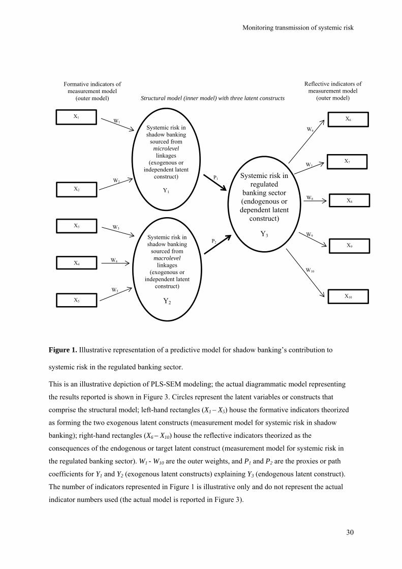
Monitoring transmission of systemic risk
30
Figure 1. Illustrative representation of a predictive model for shadow banking’s contribution to
systemic risk in the regulated banking sector.
This is an illustrative depiction of PLS-SEM modeling; the actual diagrammatic model representing
the results reported is shown in Figure 3. Circles represent the latent variables or constructs that
comprise the structural model; left-hand rectangles (X1 – X5) house the formative indicators theorized
as forming the two exogenous latent constructs (measurement model for systemic risk in shadow
banking); right-hand rectangles (X6 – X10) house the reflective indicators theorized as the
consequences of the endogenous or target latent construct (measurement model for systemic risk in
the regulated banking sector). W1 - W10 are the outer weights, and P1 and P2 are the proxies or path
coefficients for Y1 and Y2 (exogenous latent constructs) explaining Y3 (endogenous latent construct).
The number of indicators represented in Figure 1 is illustrative only and do not represent the actual
indicator numbers used (the actual model is reported in Figure 3).
Formative indicators of measurement model
(outer model)
X2
X3
X4
X5
Systemic risk in regulated
banking sector (endogenous or dependent latent
construct)
Y3Systemic risk in shadow banking
sourced from macrolevel
linkages (exogenous or
independent latent construct)
Y2X10
X8
X6 X1
X9
Reflective indicators of measurement model
(outer model) Structural model (inner model) with three latent constructs
Systemic risk in shadow banking
sourced from microlevel linkages
(exogenous or independent latent
construct)
Y1
W1
P1 W2
P2
X7
W10
W9
W8
W4
W3
W5
W6
W7
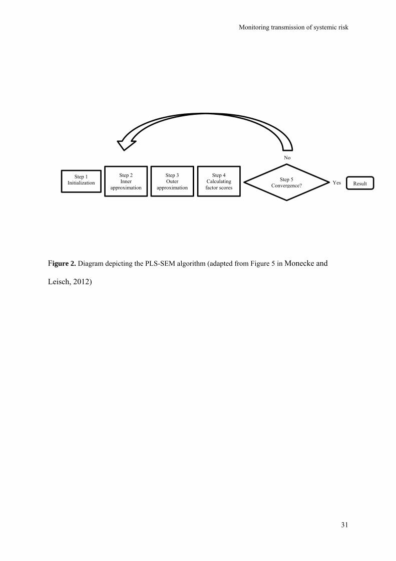
Monitoring transmission of systemic risk
31
Figure 2. Diagram depicting the PLS-SEM algorithm (adapted from Figure 5 in Monecke and
Leisch, 2012)
ResultStep 1
Initialization Step 5
Convergence?
Step 2 Inner
approximation
Step 3 Outer
approximation
Step 4 Calculating factor scores
No
Yes
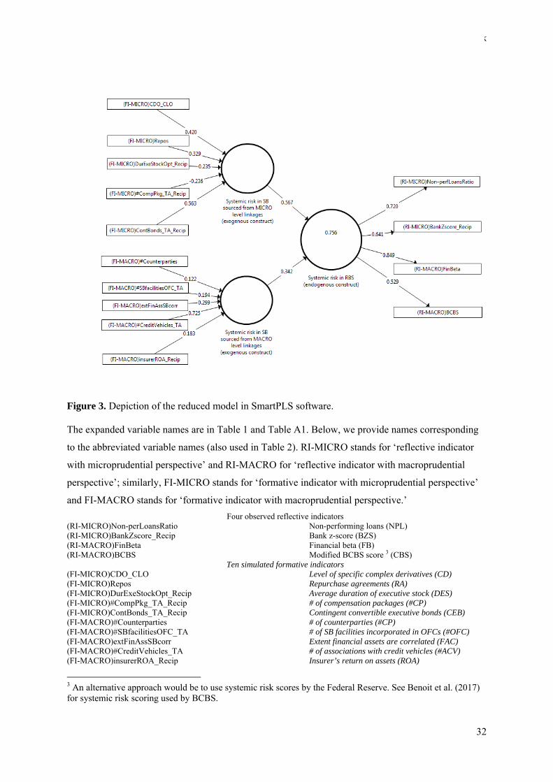
Monitoring transmission of systemic risk
32
Figure 3. Depiction of the reduced model in SmartPLS software.
The expanded variable names are in Table 1 and Table A1. Below, we provide names corresponding
to the abbreviated variable names (also used in Table 2). RI-MICRO stands for ‘reflective indicator
with microprudential perspective’ and RI-MACRO for ‘reflective indicator with macroprudential
perspective’; similarly, FI-MICRO stands for ‘formative indicator with microprudential perspective’
and FI-MACRO stands for ‘formative indicator with macroprudential perspective.’
Four observed reflective indicators (RI-MICRO)Non-perLoansRatio Non-performing loans (NPL) (RI-MICRO)BankZscore_Recip Bank z-score (BZS) (RI-MACRO)FinBeta Financial beta (FB) (RI-MACRO)BCBS Modified BCBS score 3 (CBS)
Ten simulated formative indicators (FI-MICRO)CDO_CLO Level of specific complex derivatives (CD) (FI-MICRO)Repos Repurchase agreements (RA) (FI-MICRO)DurExeStockOpt_Recip Average duration of executive stock (DES) (FI-MICRO)#CompPkg_TA_Recip # of compensation packages (#CP) (FI-MICRO)ContBonds_TA_Recip Contingent convertible executive bonds (CEB) (FI-MACRO)#Counterparties # of counterparties (#CP) (FI-MACRO)#SBfacilitiesOFC_TA # of SB facilities incorporated in OFCs (#OFC) (FI-MACRO)extFinAssSBcorr Extent financial assets are correlated (FAC) (FI-MACRO)#CreditVehicles_TA # of associations with credit vehicles (#ACV) (FI-MACRO)insurerROA_Recip Insurer’s return on assets (ROA)
3 An alternative approach would be to use systemic risk scores by the Federal Reserve. See Benoit et al. (2017) for systemic risk scoring used by BCBS.
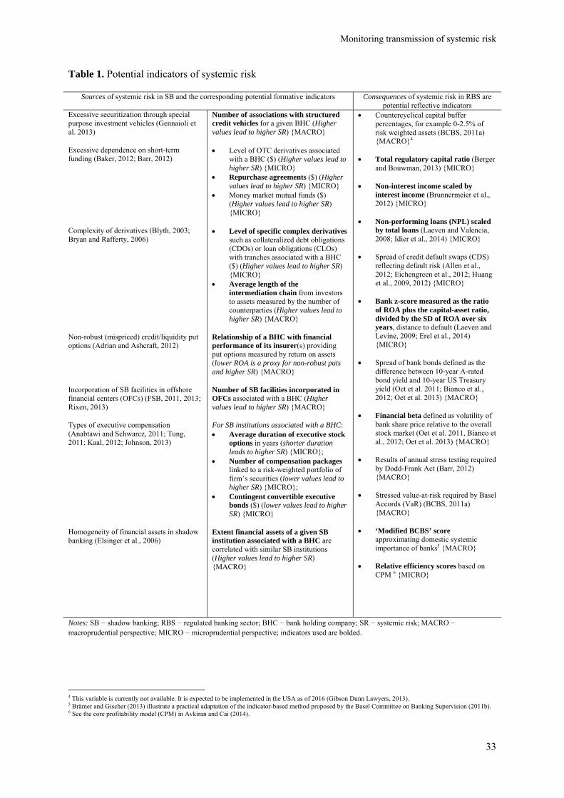
Monitoring transmission of systemic risk
33
Table 1. Potential indicators of systemic risk
Sources of systemic risk in SB and the corresponding potential formative indicators Consequences of systemic risk in RBS are potential reflective indicators
Excessive securitization through special purpose investment vehicles (Gennaioli et al. 2013)
Number of associations with structured credit vehicles for a given BHC (Higher values lead to higher SR) {MACRO}
Countercyclical capital buffer percentages, for example 0-2.5% of risk weighted assets (BCBS, 2011a) {MACRO}4
Total regulatory capital ratio (Berger
and Bouwman, 2013) {MICRO} Non-interest income scaled by
interest income (Brunnermeier et al., 2012) {MICRO}
Non-performing loans (NPL) scaled
by total loans (Laeven and Valencia, 2008; Idier et al., 2014) {MICRO}
Spread of credit default swaps (CDS)
reflecting default risk (Allen et al., 2012; Eichengreen et al., 2012; Huang et al., 2009, 2012) {MICRO}
Bank z-score measured as the ratio
of ROA plus the capital-asset ratio, divided by the SD of ROA over six years, distance to default (Laeven and Levine, 2009; Erel et al., 2014) {MICRO}
Spread of bank bonds defined as the
difference between 10-year A-rated bond yield and 10-year US Treasury yield (Oet et al. 2011; Bianco et al., 2012; Oet et al. 2013) {MACRO}
Financial beta defined as volatility of
bank share price relative to the overall stock market (Oet et al. 2011, Bianco et al., 2012; Oet et al. 2013) {MACRO}
Results of annual stress testing required
by Dodd-Frank Act (Barr, 2012) {MACRO}
Stressed value-at-risk required by Basel
Accords (VaR) (BCBS, 2011a) {MACRO}
‘Modified BCBS’ score
approximating domestic systemic importance of banks5 {MACRO}
Relative efficiency scores based on
CPM 6 {MICRO}
Excessive dependence on short-term funding (Baker, 2012; Barr, 2012)
Level of OTC derivatives associated with a BHC ($) (Higher values lead to higher SR) {MICRO}
Repurchase agreements ($) (Higher values lead to higher SR) {MICRO}
Money market mutual funds ($) (Higher values lead to higher SR) {MICRO}
Complexity of derivatives (Blyth, 2003; Bryan and Rafferty, 2006)
Level of specific complex derivatives such as collateralized debt obligations (CDOs) or loan obligations (CLOs) with tranches associated with a BHC ($) (Higher values lead to higher SR) {MICRO}
Average length of the intermediation chain from investors to assets measured by the number of counterparties (Higher values lead to higher SR) {MACRO}
Non-robust (mispriced) credit/liquidity put options (Adrian and Ashcraft, 2012)
Relationship of a BHC with financial performance of its insurer(s) providing put options measured by return on assets (lower ROA is a proxy for non-robust puts and higher SR) {MACRO}
Incorporation of SB facilities in offshore financial centers (OFCs) (FSB, 2011, 2013; Rixen, 2013)
Number of SB facilities incorporated in OFCs associated with a BHC (Higher values lead to higher SR) {MACRO}
Types of executive compensation (Anabtawi and Schwarcz, 2011; Tung, 2011; Kaal, 2012; Johnson, 2013)
For SB institutions associated with a BHC: Average duration of executive stock
options in years (shorter duration leads to higher SR) {MICRO};
Number of compensation packages linked to a risk-weighted portfolio of firm’s securities (lower values lead to higher SR) {MICRO};
Contingent convertible executive bonds ($) (lower values lead to higher SR) {MICRO}
Homogeneity of financial assets in shadow banking (Elsinger et al., 2006)
Extent financial assets of a given SB institution associated with a BHC are correlated with similar SB institutions (Higher values lead to higher SR) {MACRO}
Notes: SB – shadow banking; RBS – regulated banking sector; BHC – bank holding company; SR – systemic risk; MACRO – macroprudential perspective; MICRO – microprudential perspective; indicators used are bolded.
4 This variable is currently not available. It is expected to be implemented in the USA as of 2016 (Gibson Dunn Lawyers, 2013). 5 Brämer and Gischer (2013) illustrate a practical adaptation of the indicator-based method proposed by the Basel Committee on Banking Supervision (2011b). 6 See the core profitability model (CPM) in Avkiran and Cai (2014).
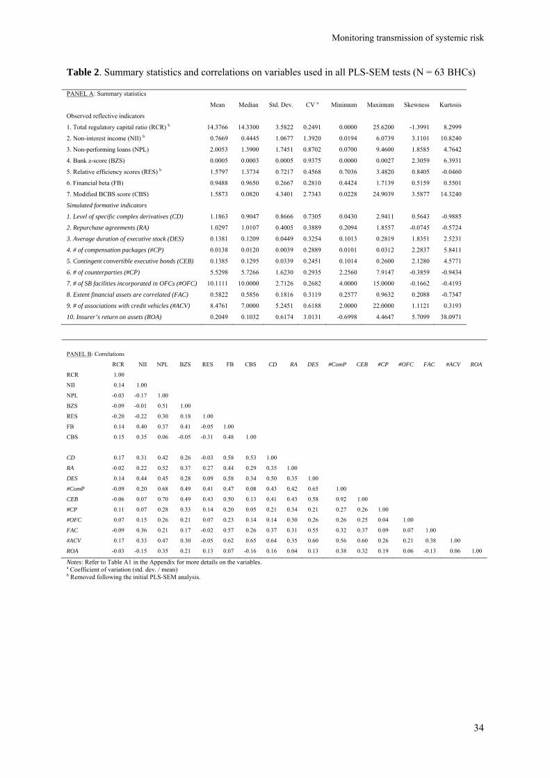
Monitoring transmission of systemic risk
34
Table 2. Summary statistics and correlations on variables used in all PLS-SEM tests (N = 63 BHCs)
PANEL A: Summary statistics
Mean Median Std. Dev. CV a Minimum Maximum Skewness
Kurtosis
Observed reflective indicators
1. Total regulatory capital ratio (RCR) b 14.3766 14.3300 3.5822 0.2491 0.0000 25.6200 -1.3991 8.2999
2. Non-interest income (NII) b 0.7669 0.4445 1.0677 1.3920 0.0194 6.0739 3.1101 10.8240
3. Non-performing loans (NPL) 2.0053 1.3900 1.7451 0.8702 0.0700 9.4600 1.8585 4.7642
4. Bank z-score (BZS) 0.0005 0.0003 0.0005 0.9375 0.0000 0.0027 2.3059 6.3931
5. Relative efficiency scores (RES) b 1.5797 1.3734 0.7217 0.4568 0.7036 3.4820 0.8405 -0.0460
6. Financial beta (FB) 0.9488 0.9650 0.2667 0.2810 0.4424 1.7139 0.5159 0.5501
7. Modified BCBS score (CBS) 1.5873 0.0820 4.3401 2.7343 0.0228 24.9039 3.5877 14.3240
Simulated formative indicators
1. Level of specific complex derivatives (CD) 1.1863 0.9047 0.8666 0.7305 0.0430 2.9411 0.5643 -0.9885
2. Repurchase agreements (RA) 1.0297 1.0107 0.4005 0.3889 0.2094 1.8557 -0.0745 -0.5724
3. Average duration of executive stock (DES) 0.1381 0.1209 0.0449 0.3254 0.1013 0.2819 1.8351 2.5231
4. # of compensation packages (#CP) 0.0138 0.0120 0.0039 0.2889 0.0101 0.0312 2.2837 5.8411
5. Contingent convertible executive bonds (CEB) 0.1385 0.1295 0.0339 0.2451 0.1014 0.2600 2.1280 4.5771
6. # of counterparties (#CP) 5.5298 5.7266 1.6230 0.2935 2.2560 7.9147 -0.3859 -0.9434
7. # of SB facilities incorporated in OFCs (#OFC) 10.1111 10.0000 2.7126 0.2682 4.0000 15.0000 -0.1662 -0.4193
8. Extent financial assets are correlated (FAC) 0.5822 0.5856 0.1816 0.3119 0.2577 0.9632 0.2088 -0.7347
9. # of associations with credit vehicles (#ACV) 8.4761 7.0000 5.2451 0.6188 2.0000 22.0000 1.1121 0.3193
10. Insurer’s return on assets (ROA) 0.2049 0.1032 0.6174 3.0131 -0.6998 4.4647 5.7099 38.0971
PANEL B: Correlations
RCR NII NPL BZS RES FB CBS CD RA DES #ComP CEB #CP #OFC FAC #ACV ROA
RCR 1.00
NII 0.14 1.00
NPL -0.03 -0.17 1.00
BZS -0.09 -0.01 0.51 1.00
RES -0.20 -0.22 0.30 0.18 1.00
FB 0.14 0.40 0.37 0.41 -0.05 1.00
CBS 0.15 0.35 0.06 -0.05 -0.31 0.48 1.00
CD 0.17 0.31 0.42 0.26 -0.03 0.58 0.53 1.00
RA -0.02 0.22 0.52 0.37 0.27 0.44 0.29 0.35 1.00
DES 0.14 0.44 0.45 0.28 0.09 0.58 0.34 0.50 0.35 1.00
#ComP -0.09 0.20 0.68 0.49 0.41 0.47 0.08 0.43 0.42 0.65 1.00
CEB -0.06 0.07 0.70 0.49 0.43 0.50 0.13 0.41 0.43 0.58 0.92 1.00
#CP 0.11 0.07 0.28 0.33 0.14 0.20 0.05 0.21 0.34 0.21 0.27 0.26 1.00
#OFC 0.07 0.15 0.26 0.21 0.07 0.23 0.14 0.14 0.30 0.26 0.26 0.25 0.04 1.00
FAC -0.09 0.36 0.21 0.17 -0.02 0.57 0.26 0.37 0.31 0.55 0.32 0.37 0.09 0.07 1.00
#ACV 0.17 0.33 0.47 0.30 -0.05 0.62 0.65 0.64 0.35 0.60 0.56 0.60 0.26 0.21 0.38 1.00
ROA -0.03 -0.15 0.35 0.21 0.13 0.07 -0.16 0.16 0.04 0.13 0.38 0.32 0.19 0.06 -0.13 0.06 1.00
Notes: Refer to Table A1 in the Appendix for more details on the variables. a Coefficient of variation (std. dev. / mean) b Removed following the initial PLS-SEM analysis.
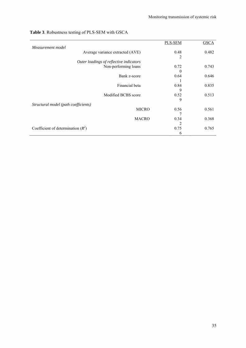
Monitoring transmission of systemic risk
35
Table 3. Robustness testing of PLS-SEM with GSCA
PLS-SEM GSCA Measurement model
Average variance extracted (AVE) 0.482
0.482
Outer loadings of reflective indicators Non-performing loans 0.72
0 0.743
Bank z-score 0.641
0.646
Financial beta 0.849
0.835
Modified BCBS score 0.529
0.513
Structural model (path coefficients) MICRO 0.56
7 0.561
MACRO 0.342
0.368
Coefficient of determination (R2) 0.756
0.765
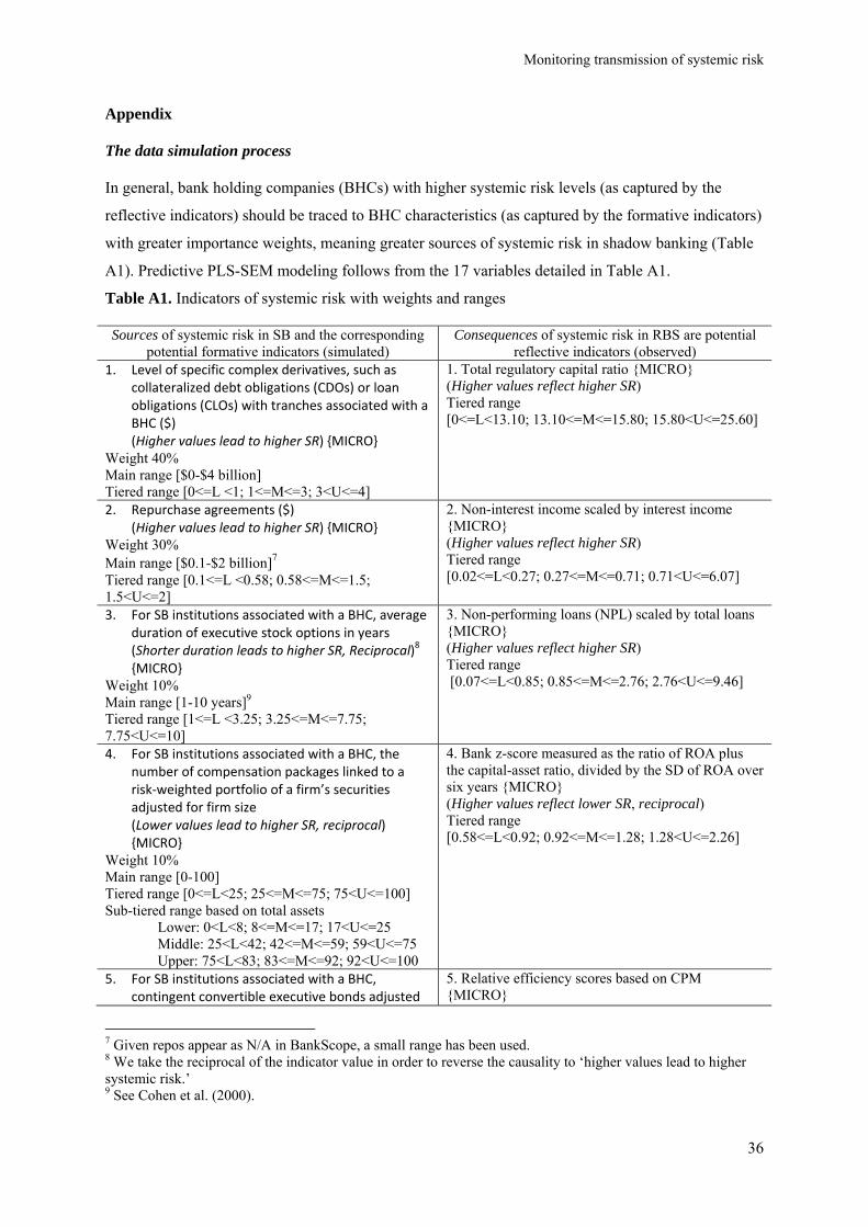
Monitoring transmission of systemic risk
36
Appendix
The data simulation process
In general, bank holding companies (BHCs) with higher systemic risk levels (as captured by the
reflective indicators) should be traced to BHC characteristics (as captured by the formative indicators)
with greater importance weights, meaning greater sources of systemic risk in shadow banking (Table
A1). Predictive PLS-SEM modeling follows from the 17 variables detailed in Table A1.
Table A1. Indicators of systemic risk with weights and ranges
Sources of systemic risk in SB and the corresponding potential formative indicators (simulated)
Consequences of systemic risk in RBS are potential reflective indicators (observed)
1. Level of specific complex derivatives, such as collateralized debt obligations (CDOs) or loan obligations (CLOs) with tranches associated with a BHC ($) (Higher values lead to higher SR) {MICRO}
Weight 40% Main range [$0-$4 billion] Tiered range [0<=L <1; 1<=M<=3; 3<U<=4]
1. Total regulatory capital ratio {MICRO} (Higher values reflect higher SR) Tiered range [0<=L<13.10; 13.10<=M<=15.80; 15.80<U<=25.60]
2. Repurchase agreements ($) (Higher values lead to higher SR) {MICRO}
Weight 30% Main range [$0.1-$2 billion]7 Tiered range [0.1<=L <0.58; 0.58<=M<=1.5; 1.5<U<=2]
2. Non-interest income scaled by interest income {MICRO} (Higher values reflect higher SR) Tiered range [0.02<=L<0.27; 0.27<=M<=0.71; 0.71<U<=6.07]
3. For SB institutions associated with a BHC, average duration of executive stock options in years (Shorter duration leads to higher SR, Reciprocal)8 {MICRO}
Weight 10% Main range [1-10 years]9 Tiered range [1<=L <3.25; 3.25<=M<=7.75; 7.75<U<=10]
3. Non-performing loans (NPL) scaled by total loans {MICRO} (Higher values reflect higher SR) Tiered range [0.07<=L<0.85; 0.85<=M<=2.76; 2.76<U<=9.46]
4. For SB institutions associated with a BHC, the number of compensation packages linked to a risk‐weighted portfolio of a firm’s securities adjusted for firm size (Lower values lead to higher SR, reciprocal) {MICRO}
Weight 10% Main range [0-100] Tiered range [0<=L<25; 25<=M<=75; 75<U<=100] Sub-tiered range based on total assets
Lower: 0<L<8; 8<=M<=17; 17<U<=25 Middle: 25<L<42; 42<=M<=59; 59<U<=75
Upper: 75<L<83; 83<=M<=92; 92<U<=100
4. Bank z-score measured as the ratio of ROA plus the capital-asset ratio, divided by the SD of ROA over six years {MICRO} (Higher values reflect lower SR, reciprocal) Tiered range [0.58<=L<0.92; 0.92<=M<=1.28; 1.28<U<=2.26]
5. For SB institutions associated with a BHC, contingent convertible executive bonds adjusted
5. Relative efficiency scores based on CPM {MICRO}
7 Given repos appear as N/A in BankScope, a small range has been used. 8 We take the reciprocal of the indicator value in order to reverse the causality to ‘higher values lead to higher systemic risk.’ 9 See Cohen et al. (2000).
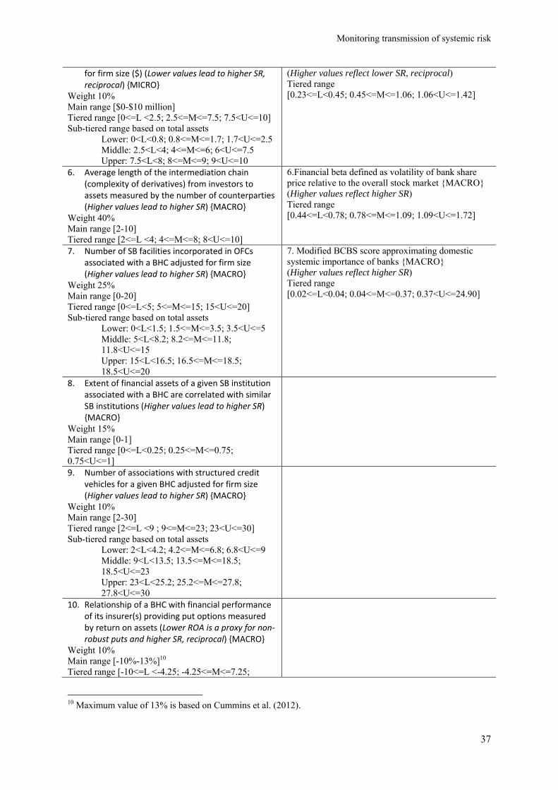
Monitoring transmission of systemic risk
37
for firm size ($) (Lower values lead to higher SR,reciprocal) {MICRO}
Weight 10% Main range [$0-$10 million] Tiered range [0<=L <2.5; 2.5<=M<=7.5; 7.5<U<=10] Sub-tiered range based on total assets
Lower: 0<L<0.8; 0.8<=M<=1.7; 1.7<U<=2.5 Middle: 2.5<L<4; 4<=M<=6; 6<U<=7.5
Upper: 7.5<L<8; 8<=M<=9; 9<U<=10
(Higher values reflect lower SR, reciprocal) Tiered range [0.23<=L<0.45; 0.45<=M<=1.06; 1.06<U<=1.42]
6. Average length of the intermediation chain (complexity of derivatives) from investors to assets measured by the number of counterparties (Higher values lead to higher SR) {MACRO}
Weight 40% Main range [2-10] Tiered range [2<=L <4; 4<=M<=8; 8<U<=10]
6.Financial beta defined as volatility of bank share price relative to the overall stock market {MACRO} (Higher values reflect higher SR) Tiered range [0.44<=L<0.78; 0.78<=M<=1.09; 1.09<U<=1.72]
7. Number of SB facilities incorporated in OFCs associated with a BHC adjusted for firm size (Higher values lead to higher SR) {MACRO}
Weight 25% Main range [0-20] Tiered range [0<=L<5; 5<=M<=15; 15<U<=20] Sub-tiered range based on total assets
Lower: 0<L<1.5; 1.5<=M<=3.5; 3.5<U<=5 Middle: 5<L<8.2; 8.2<=M<=11.8; 11.8<U<=15 Upper: 15<L<16.5; 16.5<=M<=18.5; 18.5<U<=20
7. Modified BCBS score approximating domestic systemic importance of banks {MACRO} (Higher values reflect higher SR) Tiered range [0.02<=L<0.04; 0.04<=M<=0.37; 0.37<U<=24.90]
8. Extent of financial assets of a given SB institution associated with a BHC are correlated with similar SB institutions (Higher values lead to higher SR) {MACRO}
Weight 15% Main range [0-1] Tiered range [0<=L<0.25; 0.25<=M<=0.75; 0.75<U<=1]
9. Number of associations with structured credit vehicles for a given BHC adjusted for firm size (Higher values lead to higher SR) {MACRO}
Weight 10% Main range [2-30] Tiered range [2<=L <9 ; 9<=M<=23; 23<U<=30] Sub-tiered range based on total assets
Lower: 2<L<4.2; 4.2<=M<=6.8; 6.8<U<=9 Middle: 9<L<13.5; 13.5<=M<=18.5; 18.5<U<=23 Upper: 23<L<25.2; 25.2<=M<=27.8; 27.8<U<=30
10. Relationship of a BHC with financial performance of its insurer(s) providing put options measured by return on assets (Lower ROA is a proxy for non‐robust puts and higher SR, reciprocal) {MACRO}
Weight 10% Main range [-10%-13%]10 Tiered range [-10<=L <-4.25; -4.25<=M<=7.25;
10 Maximum value of 13% is based on Cummins et al. (2012).
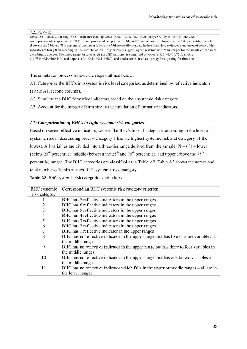
Monitoring transmission of systemic risk
38
7.25<U<=13] Notes: SB – shadow banking; RBS – regulated banking sector; BHC – bank holding company; SR – systemic risk; MACRO – macroprudential perspective; MICRO – microprudential perspective. L, M, and U are notations for lower (below 25th percentile), middle (between the 25th and 75th percentile) and upper (above the 75th percentile) ranges. In the simulation, reciprocals are taken of some of the indicators to bring their meaning in line with the others – higher levels suggest higher systemic risk. Main ranges for the simulated variables are arbitrary choices. The tiered range for total assets (in USD millions) is comprised of lower (8,735<=L<14,751), middle (14,751<=M<=100,440), and upper (100,440<U<=2,415,689), and total assets is used as a proxy for adjusting for firm size.
The simulation process follows the steps outlined below:
A1. Categorize the BHCs into systemic risk level categories, as determined by reflective indicators
(Table A1, second column).
A2. Simulate the BHC formative indicators based on their systemic risk category.
A3. Account for the impact of firm size in the simulation of formative indicators.
A1: Categorization of BHCs in eight systemic risk categories
Based on seven reflective indicators, we sort the BHCs into 11 categories according to the level of
systemic risk in descending order – Category 1 has the highest systemic risk and Category 11 the
lowest. All variables are divided into a three-tier range derived from the sample (N = 63) – lower
(below 25th percentile), middle (between the 25th and 75th percentile), and upper (above the 75th
percentile) ranges. The BHC categories are classified as in Table A2. Table A3 shows the names and
total number of banks in each BHC systemic risk category.
Table A2. BHC systemic risk categories and criteria
BHC systemic risk category
Corresponding BHC systemic risk category criterion
1 BHC has 7 reflective indicators in the upper ranges 2 BHC has 6 reflective indicators in the upper ranges 3 BHC has 5 reflective indicators in the upper ranges 4 BHC has 4 reflective indicators in the upper ranges 5 BHC has 3 reflective indicators in the upper ranges 6 BHC has 2 reflective indicators in the upper ranges 7 BHC has 1 reflective indicator in the upper ranges 8 BHC has no reflective indicator in the upper range, but has five or more variables in
the middle ranges 9 BHC has no reflective indicator in the upper range but has three to four variables in
the middle ranges 10 BHC has no reflective indicator in the upper range, but has one to two variables in
the middle ranges 11 BHC has no reflective indicator which falls in the upper or middle ranges – all are in
the lower ranges
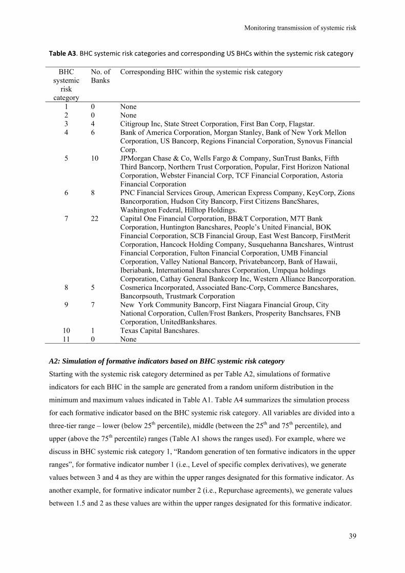
Monitoring transmission of systemic risk
39
Table A3. BHC systemic risk categories and corresponding US BHCs within the systemic risk category
BHC systemic
risk category
No. of Banks
Corresponding BHC within the systemic risk category
1 0 None 2 0 None 3 4 Citigroup Inc, State Street Corporation, First Ban Corp, Flagstar. 4 6 Bank of America Corporation, Morgan Stanley, Bank of New York Mellon
Corporation, US Bancorp, Regions Financial Corporation, Synovus Financial Corp.
5 10 JPMorgan Chase & Co, Wells Fargo & Company, SunTrust Banks, Fifth Third Bancorp, Northern Trust Corporation, Popular, First Horizon National Corporation, Webster Financial Corp, TCF Financial Corporation, Astoria Financial Corporation
6 8 PNC Financial Services Group, American Express Company, KeyCorp, Zions Bancorporation, Hudson City Bancorp, First Citizens BancShares, Washington Federal, Hilltop Holdings.
7 22 Capital One Financial Corporation, BB&T Corporation, M7T Bank Corporation, Huntington Bancshares, People’s United Financial, BOK Financial Corporation, SCB Financial Group, East West Bancorp, FirstMerit Corporation, Hancock Holding Company, Susquehanna Bancshares, Wintrust Financial Corporation, Fulton Financial Corporation, UMB Financial Corporation, Valley National Bancorp, Privatebancorp, Bank of Hawaii, Iberiabank, International Bancshares Corporation, Umpqua holdings Corporation, Cathay General Bankcorp Inc, Western Alliance Bancorporation.
8 5 Cosmerica Incorporated, Associated Banc-Corp, Commerce Bancshares, Bancorpsouth, Trustmark Corporation
9 7 New York Community Bancorp, First Niagara Financial Group, City National Corporation, Cullen/Frost Bankers, Prosperity Banchsares, FNB Corporation, UnitedBankshares.
10 1 Texas Capital Bancshares. 11 0 None
A2: Simulation of formative indicators based on BHC systemic risk category
Starting with the systemic risk category determined as per Table A2, simulations of formative
indicators for each BHC in the sample are generated from a random uniform distribution in the
minimum and maximum values indicated in Table A1. Table A4 summarizes the simulation process
for each formative indicator based on the BHC systemic risk category. All variables are divided into a
three-tier range – lower (below 25th percentile), middle (between the 25th and 75th percentile), and
upper (above the 75th percentile) ranges (Table A1 shows the ranges used). For example, where we
discuss in BHC systemic risk category 1, “Random generation of ten formative indicators in the upper
ranges”, for formative indicator number 1 (i.e., Level of specific complex derivatives), we generate
values between 3 and 4 as they are within the upper ranges designated for this formative indicator. As
another example, for formative indicator number 2 (i.e., Repurchase agreements), we generate values
between 1.5 and 2 as these values are within the upper ranges designated for this formative indicator.
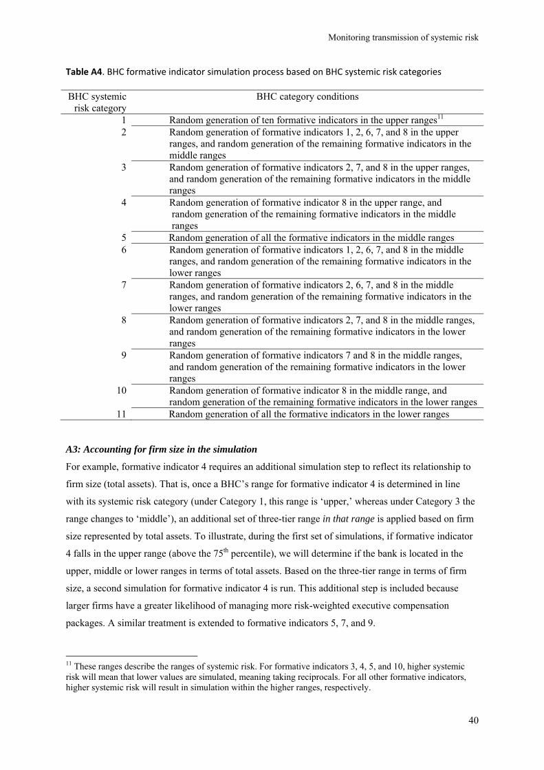
Monitoring transmission of systemic risk
40
Table A4. BHC formative indicator simulation process based on BHC systemic risk categories
BHC systemic risk category
BHC category conditions
1 Random generation of ten formative indicators in the upper ranges11 2 Random generation of formative indicators 1, 2, 6, 7, and 8 in the upper
ranges, and random generation of the remaining formative indicators in the middle ranges
3 Random generation of formative indicators 2, 7, and 8 in the upper ranges, and random generation of the remaining formative indicators in the middle ranges
4 Random generation of formative indicator 8 in the upper range, and random generation of the remaining formative indicators in the middle ranges
5 Random generation of all the formative indicators in the middle ranges 6 Random generation of formative indicators 1, 2, 6, 7, and 8 in the middle
ranges, and random generation of the remaining formative indicators in the lower ranges
7 Random generation of formative indicators 2, 6, 7, and 8 in the middle ranges, and random generation of the remaining formative indicators in the lower ranges
8 Random generation of formative indicators 2, 7, and 8 in the middle ranges, and random generation of the remaining formative indicators in the lower ranges
9 Random generation of formative indicators 7 and 8 in the middle ranges, and random generation of the remaining formative indicators in the lower ranges
10 Random generation of formative indicator 8 in the middle range, and random generation of the remaining formative indicators in the lower ranges
11 Random generation of all the formative indicators in the lower ranges
A3: Accounting for firm size in the simulation
For example, formative indicator 4 requires an additional simulation step to reflect its relationship to
firm size (total assets). That is, once a BHC’s range for formative indicator 4 is determined in line
with its systemic risk category (under Category 1, this range is ‘upper,’ whereas under Category 3 the
range changes to ‘middle’), an additional set of three-tier range in that range is applied based on firm
size represented by total assets. To illustrate, during the first set of simulations, if formative indicator
4 falls in the upper range (above the 75th percentile), we will determine if the bank is located in the
upper, middle or lower ranges in terms of total assets. Based on the three-tier range in terms of firm
size, a second simulation for formative indicator 4 is run. This additional step is included because
larger firms have a greater likelihood of managing more risk-weighted executive compensation
packages. A similar treatment is extended to formative indicators 5, 7, and 9.
11 These ranges describe the ranges of systemic risk. For formative indicators 3, 4, 5, and 10, higher systemic risk will mean that lower values are simulated, meaning taking reciprocals. For all other formative indicators, higher systemic risk will result in simulation within the higher ranges, respectively.