Embed Size (px)
Citation preview

HAL Id: hal-00795547https://hal-essec.archives-ouvertes.fr/hal-00795547
Submitted on 28 Feb 2013
HAL is a multi-disciplinary open accessarchive for the deposit and dissemination of sci-entific research documents, whether they are pub-lished or not. The documents may come fromteaching and research institutions in France orabroad, or from public or private research centers.
L’archive ouverte pluridisciplinaire HAL, estdestinée au dépôt et à la diffusion de documentsscientifiques de niveau recherche, publiés ou non,émanant des établissements d’enseignement et derecherche français ou étrangers, des laboratoirespublics ou privés.
Money in the Production Function : A New KeynesianDSGE Perspective
Jonathan Benchimol
To cite this version:Jonathan Benchimol. Money in the Production Function : A New Keynesian DSGE Perspective.ESSEC Working paper. Document de Recherche ESSEC / Centre de recherche de l’ESSEC. ISSN :1291-9616. WP 1304. 2011. <hal-00795547>

Research Center ESSEC Working Paper 1304
2013
Jonathan Benchimol
Money in the Production Function: A New Keynesian DSGE Perspective
Money in the production function: a
new Keynesian DSGE perspective�
Jonathan Benchimoly
This version: December 8th, 2011
First version: June 27th, 2010
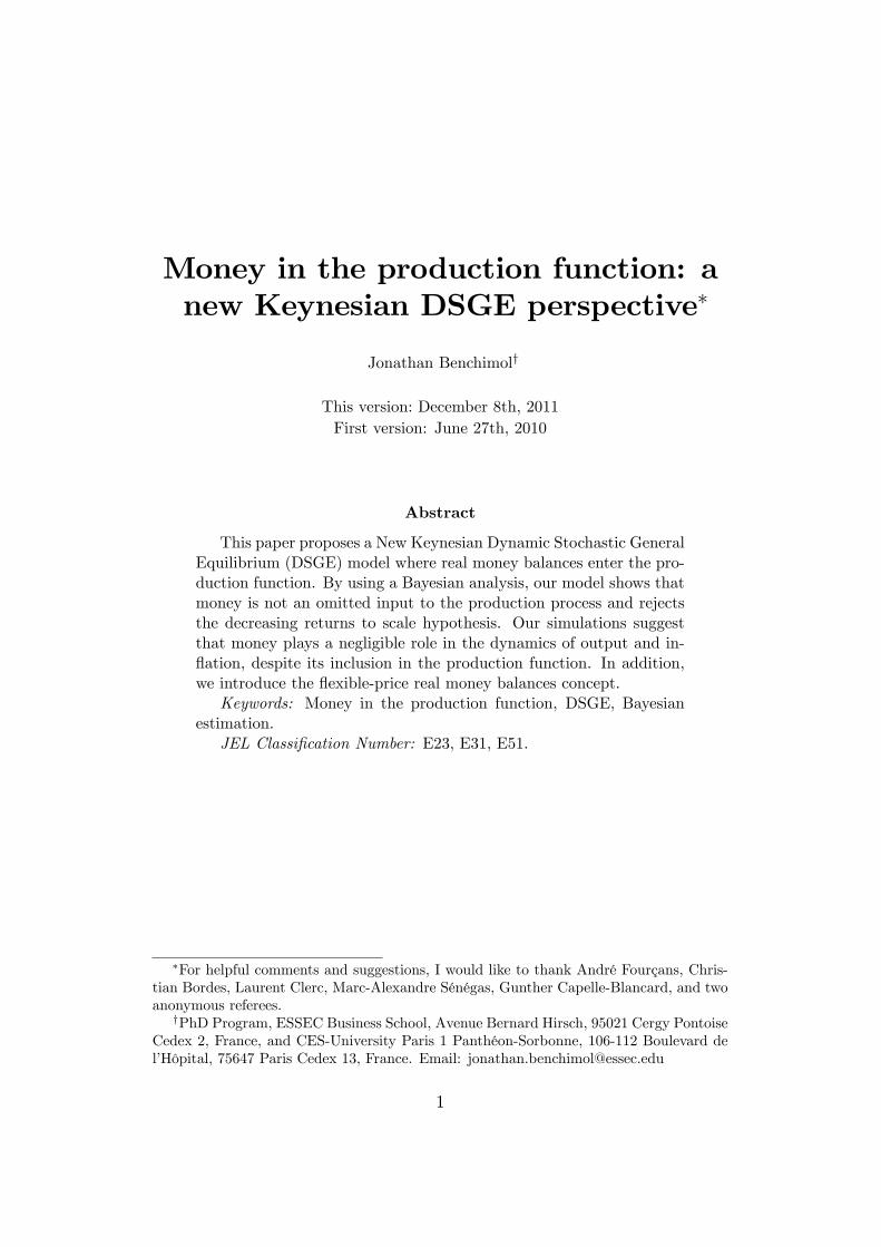
Abstract
This paper proposes a New Keynesian Dynamic Stochastic GeneralEquilibrium (DSGE) model where real money balances enter the pro-duction function. By using a Bayesian analysis, our model shows thatmoney is not an omitted input to the production process and rejectsthe decreasing returns to scale hypothesis. Our simulations suggestthat money plays a negligible role in the dynamics of output and in-�ation, despite its inclusion in the production function. In addition,we introduce the �exible-price real money balances concept.Keywords: Money in the production function, DSGE, Bayesian
estimation.JEL Classi�cation Number: E23, E31, E51.
�For helpful comments and suggestions, I would like to thank André Fourçans, Chris-tian Bordes, Laurent Clerc, Marc-Alexandre Sénégas, Gunther Capelle-Blancard, and twoanonymous referees.
yPhD Program, ESSEC Business School, Avenue Bernard Hirsch, 95021 Cergy PontoiseCedex 2, France, and CES-University Paris 1 Panthéon-Sorbonne, 106-112 Boulevard del�Hôpital, 75647 Paris Cedex 13, France. Email: [email protected]
1

1 Introduction
The theoretical motivation for empirical implementations of money in theproduction function originates from monetary growth models of Levhari andPatinkin (1968), Friedman (1969), Johnson (1969) and Stein (1970), whichinclude money directly in the production function. Firms hold money tofacilitate production, on the grounds that money enables them to economizethe use of other inputs, and spares the cost of running short of cash (Fischer,1974).
Real cash balances are at least in part a factor of production.
To take a trivial example, a retailer can economize on his average
cash balances by hiring an errand boy to go to the bank on the
corner to get change for large bills tendered by customers. When
it costs ten cents per dollar per year to hold an extra dollar of
cash, there will be a greater incentive to hire the errand boy, that
is, to substitute other productive resources for cash. This will
mean both a reduction in the real �ow of services from the given
productive resources and a change in the structure of production,
since di¤erent productive activities may di¤er in cash-intensity,
just as they di¤er in labor - or land - intensity.
Milton Friedman (1969)
In an old article, Sinai and Stokes (1972) present a very interesting testof the hypothesis that money enters the production function, and they sug-gest that real balances could be a missing variable that contributes to theattribution of the unexplained residual to technological changes. Ben-Zionand Ruttan (1975) conclude that money as a factor of demand seems to playan important role in explaining induced technological changes.Short (1979) develops structural models based on Cobb and Douglas
(1928) and generalized translog production functions, both of which providea more complete theoretical framework for analyzing the role of money in theproduction process. The empirical results obtained by estimating these twomodels indicate that the relationship between real cash balances and output,even after correcting for any simultaneity bias, is positive and statisticallysigni�cant. The results suggest that it is theoretically appropriate to includea real cash balances variable as a factor input in a production function inorder to capture the productivity gains derived from using money.You (1981) �nds that the unexplained portion of output variation virtu-
ally vanishes with real balances included in the production function. Besideslabor and capital, real money balances turn out to be an important factor of
2

production, especially for developing countries. The results in Khan and Ah-mad (1985) are consistent with the hypothesis that real money balances arean important factor of production. Sephton (1988) shows that real balancesare a valid factor of production within the con�nes of a CES production func-tion. Hasan and Mahmud (1993) also support the hypothesis that money isan important factor in the production function and that there are potentialsupply side e¤ects of a change in the interest rate.Recent developments in econometrics regarding co-integration and error
correction models provide a rich environment in which the role of moneyin the production function can be reexamined. In a co-integrated space,Moghaddam (2010) presents empirical evidence indicating that di¤erent de-�nitions of money play an input role in the Cobb and Douglas (1928) pro-duction function.At the same time, Clarida et al. (1999), Woodford (2003) and Galí (2008)
develop New Keynesian Dynamic Stochastic General Equilibrium (DSGE)models to explain the dynamics of the economy. However, no studies usemoney as an input in the production function in New Keynesian DSGEmodels.This article departs from the existing theoretical and empirical literature
by specifying a New Keynesian DSGE model where money enters the produc-tion function. This feature generates a new in�ation dynamics where moneycould play a signi�cant role. Following Galí (2008), we introduce the newconcept of �exible-price real money balances in order to close the model. Wealso analyze the dynamics of the economy by using Bayesian estimations andsimulations to con�rm or reject the potential role of money in the dynamicsof the Eurozone. Moreover, this paper intends to solve the now-old contro-versial hypothesis about constant returns to scale of money in the productionfunction initiated by Sinai and Stokes (1972).Notice that in this paper, because data are available, we voluntary do not
distinguish money for productive and nonproductive use as in Benhabib etal. (2001).
After describing the theoretical set up in Section 2, we calibrate andestimate two models (constrained i.e. constant returns to scale, and uncon-strained i.e. decreasing returns to scale) of the Euro area using Bayesiantechniques in 3. Impulse response functions and variance decomposition areanalyzed in Section 4, and we solve the choice of the returns to scale hy-pothesis by comparing the two models of this paper in Section 5. Section 6concludes, and Section 7 presents additional results.
3

2 The model
The model consists of households that supply labor, purchase goods for con-sumption, and hold money and bonds, and �rms that hire labor and produceand sell di¤erentiated products in monopolistically competitive goods mar-kets. Each �rm sets the price of the good it produces, but not all �rms resettheir respective prices each period. Households and �rms behave optimally:households maximize the expected present value of utility, and �rms maxi-mize pro�ts. There is also a central bank that controls the nominal interestrate. This model is inspired by Smets and Wouters (2003), Galí (2008), andWalsh (2010).
2.1 Households
We assume a representative in�nitely-lived household, seeking to maximize
Et
"1X
k=0
CkUt+k
#(1)
where Ut is the period utility function, and C < 1 is the discount factor.We assume the existence of a continuum of goods represented by the
interval [0; 1]. The household decides how to allocate its consumption ex-penditures among the di¤erent goods. This requires that the consumptionindex, Ct, be maximized for any given level of expenditures. 8t 2 N, andconditionally on such optimal behavior, the period budget constraint takesthe form
PtCt +Mt +QtBt � Bt�1 +WtNt +Mt�1 (2)
where Pt is an aggregate price index, Mt is the quantity of money holdingsat time t, Bt is the quantity of one-period nominally riskless discount bondspurchased in period t and maturing in period t+1 (each bond pays one unitof money at maturity and its price is Qt, so that the short term nominal rateit is approximately equals to � logQt), Wt is the nominal wage, and Nt ishours of work (or the measure of household members employed).The above sequence of period budget constraints is supplemented with a
solvency condition, such as 8t limn�!1
Et [Bn] � 0.
Preferences are measured with a common time-separable utility function.Under the assumption of a period utility given by
Ut = e"pt
C1��t
1� �+De"
mt
1� �
�Mt
Pt
�1����N1+�
t
1 + �
!(3)
4

consumption, labor supply, money demand and bond holdings are chosen tomaximize (1) subject to (2) and the solvency condition. This MIU utilityfunction depends positively on the consumption of goods, Ct, positively onreal money balances, Mt
Pt, and negatively on labor Nt. � is the coe¢cient
of relative risk aversion of households or the inverse of the intertemporalelasticity of substitution, � is the inverse of the elasticity of money holdingswith respect to the interest rate, and � is the inverse of the elasticity of worke¤ort with respect to the real wage (inverse of the Frisch elasticity of laborsupply).The utility function also contains two structural shocks: "pt is a general
shock to preferences that a¤ects the intertemporal substitution of households(preference shock) and "mt is a money demand shock. D and � are positivescale parameters.This setting leads to the following conditions1, which, in addition to the
budget constraint, must hold in equilibrium. The resulting log-linear versionof the �rst order condition corresponding to the demand for contingent bondsimplies that
ct = Et [ct+1]�1
�(it � Et [�t+1]� �c)� ��1Et
��"pt+1
�(4)
where the lowercase letters denote the logarithm of the original aggregatedvariables, �c = � log (C), and � is the �rst-di¤erence operator.The demand for cash that follows from the household�s optimization prob-
lem is given by"mt + �ct � �mpt � �m = a2it (5)
where mpt = mt � pt are the log-linearized real money balances, �m =� log (D) + a1, a1 and a2 are resulting terms of the �rst-order Taylor ap-proximation of log (1�Qt) = a1 + a2it. More precisely, if we compute our�rst-order Taylor approximation around the steady-state interest rate, 1
C, we
obtain a1 = log�1� exp
�� 1C
���
1
C
e1C �1
, and a2 =1
e1C �1
.
Real cash holdings depend positively on consumption, with an elasticityequal to �=�, and negatively on the nominal interest rate ( 1
C> 1 which
implies that a2 > 0). Below, we take the nominal interest rate as the centralbank�s policy instrument.In the literature, due to the assumption that consumption and real money
balances are additively separable in the utility function, cash holdings do notenter any of the other structural equations: accordingly, the above equationbecomes a recursive function of the rest of the system of equations. However,
1See Appendix 7.A.
5

as in Sinai and Stokes (1972), Subrahmanyam (1980), or Khan and Ahmad(1985), because real money balances enter the aggregate supply, we will usethis money demand equation (eq. 5) in order to solve the equilibrium of ourmodel. See for instance Ireland (2004) and Benchimol and Fourçans (2012)for models in which money balances enter the aggregate demand equationwithout entering the production function.The resulting log-linear version of the �rst order condition corresponding
to the optimal consumption-leisure arbitrage implies that
wt � pt = �ct + �nt � �n (6)
where �n = � log (�).Finally, these equations represent the Euler condition for the optimal in-
tratemporal allocation of consumption (eq. 4), the intertemporal optimalitycondition setting the marginal rate of substitution between money and con-sumption equal to the opportunity cost of holding money (eq. 5), and theintratemporal optimality condition setting the marginal rate of substitutionbetween leisure and consumption equal to the real wage (eq. 6).
2.2 Firms
We assume a continuum of �rms indexed by i 2 [0; 1]. Each �rm produces adi¤erentiated good, but they all use an identical technology, represented bythe following money-in-the-production function
Yt (i) = At
�Mt
Pt
�BmNt (i)
1�Bn (7)
where At = exp ("at ) represents the level of technology, assumed to be com-
mon to all �rms and to evolve exogenously over time.All �rms face an identical isoelastic demand schedule, and take the ag-
gregate price level, Pt, and aggregate consumption index, Ct, as given. As inthe standard Calvo (1983) model, our generalization features monopolisticcompetition and staggered price setting. At any time t, only a fraction 1� �of �rms, with 0 < � < 1, can reset their prices optimally, while the remaining�rms index their prices to lagged in�ation.
2.3 Price dynamics
Let�s assume a set of �rms that do not reoptimize their posted price inperiod t. As in Galí (2008), using the de�nition of the aggregate price leveland the fact that all �rms that reset prices choose an identical price, P �t ,
6

leads to Pt =��P 1�"t�1 + (1� �) (P �t )
1�"� 1
1�" . Dividing both sides by Pt�1 andlog-linearizing around P �t = Pt�1 yields
�t = (1� �) (p�t � pt�1) (8)
In this set up, we do not assume inertial dynamics of prices. In�ationresults from the fact that �rms reoptimizing their price plans in any givenperiod, choose a price that di¤ers from the economy�s average price in theprevious period.
2.4 Price setting
A �rm reoptimizing in period t chooses the price P �t that maximizes the cur-rent market value of the pro�ts generated while that price remains e¤ective.We solve this problem to obtain a �rst-order Taylor expansion around thezero in�ation steady state of the �rm�s �rst-order condition, which leads to
p�t � pt�1 = (1� C�)
1X
k=0
(C�)k Et�cmct+kjt + (pt+k � pt�1)
�(9)
where cmct+kjt = mct+kjt�mc denotes the log deviation of marginal cost fromits steady state value mc = ��, and � = log ("= ("� 1)) is the log of thedesired gross markup.
2.5 Equilibrium
Market clearing in the goods market requires Yt (i) = Ct (i) for all i 2 [0; 1]
and all t. Aggregate output is de�ned as Yt =�R 1
0Yt (i)
1� 1
" di� ""�1
; it fol-
lows that Yt = Ct must hold for all t. One can combine the above goodsmarket clearing condition with the consumer�s Euler equation to yield theequilibrium condition
yt = Et [yt+1]� ��1 (it � Et [�t+1]� �c)� ��1Et��"pt+1
�(10)
Market clearing in the labor market requires Nt =R 10Nt (i) di. Using (7)
leads to
Nt =
Z 1
0
0@ Yt (i)
At
�Mt
Pt
�Bm
1A
1
1�Bn
di
=
0@ Yt
At
�Mt
Pt
�Bm
1A
1
1�Bn Z 1
0
�Pt (i)
Pt
�� "1�Bn
di (11)
7

where the second equality follows from the demand schedule and the goodsmarket clearing condition. Taking logs leads to
(1� Bn)nt = yt � "at � Bmmpt + dt
where dt = (1� Bn) log
�R 10
�Pt(i)Pt
�� "1�Bn
di
�, and di is a measure of price
(and, hence, output) dispersion across �rms. Following Galí (2008), in aneighborhood of the zero in�ation steady state, dt is equal to zero up to a�rst-order approximation.Hence, one can write the following approximate relation between aggre-
gate output, employment, real money balances and technology as
yt = "at + (1� Bn)nt + Bmmpt (12)
An expression is derived for an individual �rm�s marginal cost in termsof the economy�s average real marginal cost. With the marginal product oflabor,
mpnt = log
�@Yt@Nt
�
= log
�At
�Mt
Pt
�Bm(1� Bn)Nt
�Bn
�
= "at + Bmmpt + log (1� Bn)� Bnnt
and the marginal product of real money balances,
mpmpt = log
@Yt
@Mt
Pt
!
= log
AtBm
�Mt
Pt
�Bm�1Nt
1�Bn
!
= "at + log (Bm) + (Bm � 1)mpt + (1� Bn)nt
we obtain an expression of the marginal cost
mct = (wt � pt)�mpnt �mpmpt
= wt � pt +2Bn � 1
1� Bnyt +
1� Bm � Bn1� Bn
mpt
�1
1� Bn"at � log (Bm (1� Bn))
for all t, where the second equality de�nes the economy�s average marginalproduct of labor, mpnt, and the economy�s average marginal product of real
8

money balances, mpmpt, in a way that is consistent with (12). Using thefact that mct+kjt = (wt+k � pt+k)�mpnt+kjt,
mct+kjt = (wt+k � pt+k) +2Bn � 1
1� Bnyt+kjt
+1� Bm � Bn1� Bn
mpt+k �1
1� Bn"at+k � log (Bm (1� Bn))
= mct+k +2Bn � 1
1� Bn
�yt+kjt � yt+k
�
= mct+k � "2Bn � 1
1� Bn(p�t � pt+k) (13)
where the second equality follows from the demand schedule, Ct (i) =�Pt(i)Pt
��"Ct,
combined with the market clearing condition (yt = ct).Substituting (13) into (9) and rearranging terms yields
p�t � pt�1 = (1� C�)1X
k=0
(C�)k Et
� cmct+k � "2Bn�11�Bn
(p�t � pt+k)
+ (pt+k � pt�1)
�
p�t � pt�1 = (1� C�)�1X
k=0
(C�)k Et [cmct+k] +1X
k=0
(C�)k Et [�t+k] (14)
where � = 1�Bn1�Bn+"(2Bn�1)
� 1.
Finally, combining (8) in (14) yields the in�ation equation
�t = CEt [�t+1] + �mccmct (15)
where �mc = �(1��)(1�C�)
�is strictly decreasing in the index of price stickiness,
�, in the measure of decreasing returns, Bn, and in the demand elasticity, ".Next, a relation is derived between the economy�s real marginal cost and
a measure of aggregate economic activity. Notice that, independent of thenature of price setting, average real marginal cost can be expressed as
mct = (wt � pt)�mpnt �mpmpt
= (�yt + �nt � �n) +2Bn � 1
1� Bnyt +
1� Bm � Bn1� Bn
mpt
�1
1� Bn"at � log (Bm (1� Bn))
=� (1� Bn) + � + 2Bn � 1
1� Bnyt +
1� (1 + �)Bm � Bn1� Bn
mpt (16)
�1 + �
1� Bn"at � log (Bm (1� Bn))� �n
9

where derivation of the second and third equalities makes use of the house-hold�s optimality condition (6) and the (approximate) aggregate productionrelation (12).Knowing that � > 0, Bn � 1, and � � 1, it is obvious that � (1� Bn) +
� + 2Bn � 1 > 0. However, the inequality 1 � (1 + �)Bm � Bn > 0 comingfrom (16) appears unusual. In fact, it con�rms some studies from Sinai andStokes (Sinai and Stokes, 1975; Sinai and Stokes, 1977; Sinai and Stokes,1981; Sinai and Stokes, 1989) concluding that the weight on labor is moreimportant than the weight on money (or real money balances).Furthermore, and as shown previously, under �exible prices the real mar-
ginal cost is constant and given by mc = ��. De�ning the natural level ofoutput, denoted by yft , as the equilibrium level of output under �exible prices
mc =� (1� Bn) + � + 2Bn � 1
1� Bnyft +
1� (1 + �)Bm � Bn1� Bn
mpft (17)
�1 + �
1� Bn"at � log (Bm (1� Bn))� �n
thus implyingyft = �a"
at + �mmp
ft + �c (18)
where
�ya =1 + �
� + � + (1� �)Bn � 1 + Bn
�ym =Bn + Bm (1 + �)� 1
� + � + (1� �)Bn � 1 + Bn
�yc =(1� Bn) (log (Bm (1� Bn)) + �n � �)
� + � + (1� �)Bn � 1 + Bn
From (10), we obtain an expression for the natural interest rate,
ift = �c + �Et
h�yft+1
i(19)
Then, by using (5) and (19), we obtain an expression of �exible-price realmoney balances
mpft = �a2�
�Et
h�yft+1
i+�
�yft �
a2�c + �m�
+1
�"mt (20)
Subtracting (17) from (16) yields
cmct =� (1� Bn) + � + 2Bn � 1
1� Bn
�yt � yft
�+1� (1 + �)Bm � Bn
1� Bn
�mpt �mpft
�
(21)
10
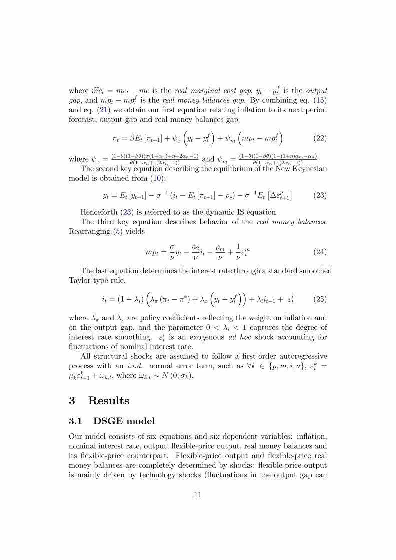
where cmct = mct � mc is the real marginal cost gap, yt � yft is the outputgap, and mpt �mpft is the real money balances gap. By combining eq. (15)and eq. (21) we obtain our �rst equation relating in�ation to its next periodforecast, output gap and real money balances gap
�t = CEt [�t+1] + x
�yt � yft
�+ m
�mpt �mpft
�(22)
where x =(1��)(1�C�)(�(1�Bn)+�+2Bn�1)
�(1�Bn+"(2Bn�1))and m =
(1��)(1�C�)(1�(1+�)Bm�Bn)�(1�Bn+"(2Bn�1))
.The second key equation describing the equilibrium of the New Keynesian
model is obtained from (10):
yt = Et [yt+1]� ��1 (it � Et [�t+1]� �c)� ��1Et��"pt+1
�(23)
Henceforth (23) is referred to as the dynamic IS equation.The third key equation describes behavior of the real money balances.
Rearranging (5) yields
mpt =�
�yt �
a2�it �
�m�+1
�"mt (24)
The last equation determines the interest rate through a standard smoothedTaylor-type rule,
it = (1� �i)��� (�t � ��) + �x
�yt � yft
��+ �iit�1 + "it (25)
where �� and �x are policy coe¢cients re�ecting the weight on in�ation andon the output gap, and the parameter 0 < �i < 1 captures the degree ofinterest rate smoothing. "it is an exogenous ad hoc shock accounting for�uctuations of nominal interest rate.All structural shocks are assumed to follow a �rst-order autoregressive
process with an i.i.d. normal error term, such as 8k 2 fp;m; i; ag, "kt =�k"
kt�1 + !k;t, where !k;t � N (0;�k).
3 Results
3.1 DSGE model
Our model consists of six equations and six dependent variables: in�ation,nominal interest rate, output, �exible-price output, real money balances andits �exible-price counterpart. Flexible-price output and �exible-price realmoney balances are completely determined by shocks: �exible-price outputis mainly driven by technology shocks (�uctuations in the output gap can
11

be attributed to supply and demand shocks), whereas the �exible-price realmoney balances are driven by money shocks and �exible-price output.
yft = �ya"at + �
ymmp
ft + �
yc (26)
mpft = �my+1Et
h�yft+1
i+ �my y
ft + �
mc +
1
�"mt (27)
�t = CEt [�t+1] + �x
�yt � yft
�+ �m
�mpt �mpft
�(28)
yt = Et [yt+1]� ��1 (it � Et [�t+1]� �c)� ��1Et��"pt+1
�(29)
mpt =�
�yt �
a2�it �
�m�+1
�"mt (30)
it = (1� �i)��� (�t � ��) + �x
�yt � yft
��+ �iit�1 + "it (31)
where
�ya =1+�
�+�+(1��)Bn�1+Bn�x =
(1��)(1�C�)(�(1�Bn)+�+2Bn�1)�(1�Bn+"(2Bn�1))
�ym =Bn+Bm(1+�)�1
�+�+(1��)Bn�1+Bn�m =
(1��)(1�C�)(1�(1+�)Bm�Bn)�(1�Bn+"(2Bn�1))
�yc =(1�Bn)(log(Bm(1�Bn))+�n�log( "
"�1))�+�+(1��)Bn�1+Bn
�m = � log (D) + a1�my+1 = �
a2��
�n = � log (�)�my =
��
�c = � log (C)
�mc = �a2�c+�m
�a1 = log
�1� e�
1
C
��
1
C
e1C �1
a2 =1
e1C �1
3.2 Euro area data
To make output and real money balances stationary, we use �rst log di¤er-ences, as in Adolfson et al. (2008). In our model of the Eurozone, �t isthe log-linearized in�ation rate measured as the yearly log di¤erence of GDPDe�ator between one quarter and the same quarter of the previous year, ytis the log-linearized output measured as the yearly log di¤erence of GDPbetween one quarter and the same quarter of the previous year, and {t isthe short-term (3-month) nominal interest rate. These data are extractedfrom the Euro area Wide Model (AWM) database of Fagan et al. (2001).cmpt is the log-linearized real money balances measured as the yearly logdi¤erence of real money between one quarter and the same quarter of theprevious year, where real money is measured as the log di¤erence betweenthe money stock and the GDP De�ator. We use theM3 monetary aggregate
12

80Q1 84Q4 89Q4 94Q4 99Q4 04Q4 09Q4- 2
0
2
4
6Output
%
80Q1 84Q4 89Q4 94Q4 99Q4 04Q4 09Q40
2
4
6
8
10
12
14Inflation
%
80Q1 84Q4 89Q4 94Q4 99Q4 04Q4 09Q4- 4
- 2
0
2
4
6
8
10Real Money Balances
%
80Q1 84Q4 89Q4 94Q4 99Q4 04Q4 09Q40
5
10
15
20Interest Rates
%
Figure 1: Euro area data (source: AWM and Eurostat)
from the Eurostat database. yft , the �exible-price output, cmpft , the �exible-price real money balances, and {ft , the �exible-price (natural) interest rate,are completely determined by structural shocks.We deal with four historical variables (Fig. 1) described latter and four
shocks: a preference shock ("pt ), a money demand shock ("mt ), a technology
shock ("at ) and a monetary policy shock ("it).
13
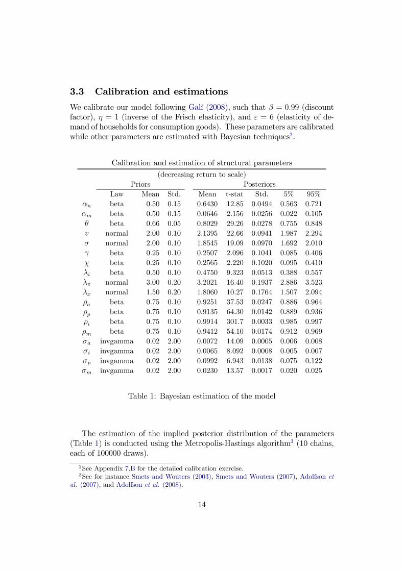
3.3 Calibration and estimations
We calibrate our model following Galí (2008), such that C = 0:99 (discountfactor), � = 1 (inverse of the Frisch elasticity), and " = 6 (elasticity of de-mand of households for consumption goods). These parameters are calibratedwhile other parameters are estimated with Bayesian techniques2.
Calibration and estimation of structural parameters
(decreasing return to scale)
Priors Posteriors
Law Mean Std. Mean t-stat Std. 5% 95%
Bn beta 0.50 0.15 0.6430 12.85 0.0494 0.563 0.721
Bm beta 0.50 0.15 0.0646 2.156 0.0256 0.022 0.105
� beta 0.66 0.05 0.8029 29.26 0.0278 0.755 0.848
v normal 2.00 0.10 2.1395 22.66 0.0941 1.987 2.294
� normal 2.00 0.10 1.8545 19.09 0.0970 1.692 2.010
D beta 0.25 0.10 0.2507 2.096 0.1041 0.085 0.406
� beta 0.25 0.10 0.2565 2.220 0.1020 0.095 0.410
�i beta 0.50 0.10 0.4750 9.323 0.0513 0.388 0.557
�� normal 3.00 0.20 3.2021 16.40 0.1937 2.886 3.523
�x normal 1.50 0.20 1.8060 10.27 0.1764 1.507 2.094
�a beta 0.75 0.10 0.9251 37.53 0.0247 0.886 0.964
�p beta 0.75 0.10 0.9135 64.30 0.0142 0.889 0.936
�i beta 0.75 0.10 0.9914 301.7 0.0033 0.985 0.997
�m beta 0.75 0.10 0.9412 54.10 0.0174 0.912 0.969
�a invgamma 0.02 2.00 0.0072 14.09 0.0005 0.006 0.008
�i invgamma 0.02 2.00 0.0065 8.092 0.0008 0.005 0.007
�p invgamma 0.02 2.00 0.0992 6.943 0.0138 0.075 0.122
�m invgamma 0.02 2.00 0.0230 13.57 0.0017 0.020 0.025
Table 1: Bayesian estimation of the model
The estimation of the implied posterior distribution of the parameters(Table 1) is conducted using the Metropolis-Hastings algorithm3 (10 chains,each of 100000 draws).
2See Appendix 7.B for the detailed calibration exercise.3See for instance Smets and Wouters (2003), Smets and Wouters (2007), Adolfson et
al. (2007), and Adolfson et al. (2008).
14

The real money balances parameter (Bm) of the augmented productionfunction is estimated to 0.064. This result is in line with Sinai and Stokes(1972). They obtain a value of 0.087 for the same parameter and they alsoconsidering M3. The prior and posterior distributions are in Appendix 7.C.1and estimates of the macro-parameters (aggregated structural parameters)are provided in Appendix 7.E.As in Table 1, we use Bayesian techniques to estimate our model with
money in the production function and a supplementary restriction. This re-striction is adopted from Short (1979) and involves the hypothesis of constantreturns to scale of the production function. Then, we assume that Bn = Bmand we test our model with this hypothesis.
Calibration and estimation of structural parameters
(constant return to scale)
Priors Posteriors
Law Mean Std. Mean t-stat Std. 5% 95%
Bn beta 0.50 0.15 0.5744 17.63 0.0320 0.519 0.625
� beta 0.66 0.05 0.8388 35.52 0.0239 0.799 0.878
v normal 2.00 0.10 2.3026 25.88 0.0887 2.158 2.450
� normal 2.00 0.10 1.7821 18.06 0.0986 1.619 1.944
D beta 0.25 0.10 0.2493 2.096 0.1041 0.085 0.403
� beta 0.25 0.10 0.2998 2.529 0.1086 0.134 0.463
�i beta 0.50 0.10 0.5432 10.74 0.0513 0.458 0.629
�� normal 3.00 0.20 3.2002 16.27 0.1955 2.876 3.515
�x normal 1.50 0.20 1.7647 10.09 0.1756 1.473 2.053
�a beta 0.75 0.10 0.9169 32.79 0.0280 0.874 0.960
�p beta 0.75 0.10 0.9056 58.20 0.0156 0.880 0.931
�i beta 0.75 0.10 0.9907 271.7 0.0037 0.984 0.997
�m beta 0.75 0.10 0.9480 57.74 0.0165 0.921 0.974
�a invgamma 0.02 2.00 0.0076 13.91 0.0005 0.006 0.008
�i invgamma 0.02 2.00 0.0059 7.101 0.0008 0.004 0.007
�p invgamma 0.02 2.00 0.0966 7.034 0.0132 0.073 0.118
�m invgamma 0.02 2.00 0.0238 13.75 0.0017 0.021 0.026
Table 2: Bayesian estimation of the model with constant return to scale
The resulting log marginal density for the model without constant returnsto scale (-512.93) and for the model with constant returns to scale (-557.52)
15

indicates that, if we admit that money enters the production function, thisproduction function should have decreasing returns to scale.Robustness diagnosis about the numerical maximization of the posterior
kernel are also computed and indicates that the optimization procedure leadsto a robust maximum for the posterior kernel. The convergence of the pro-posed distribution to the target distribution is satis�ed. A diagnosis of theoverall convergence for the Metropolis-Hastings sampling algorithm is pro-vided in Appendix 7.D.
4 Simulations
4.1 Impulse response functions
Fig. 2 presents the response of key variables to structural shocks. The thinsolid line represents the decreasing return-to-scale model responses and thedashed line represents the constant return-to-scale model responses.In response to a preference shock, the in�ation rate, the output, the
output gap, the real money balances, the nominal and the real interest ratesrise; real money growth displays a little overshooting process in the �rstperiods, then returns quickly to its steady-state value.After a technology shock, the output gap, the in�ation rate, the nominal
and the real interest rates decrease, whereas output as well as real moneybalances and real money growth rise.Following a money shock, in�ation, output, real and nominal interest
rates and the output gap dynamics di¤ers depending on the model. Themodel of decreasing returns to scale displays more coherent results than thatof constant returns to scale.In response to an interest rate shock, the in�ation rate, the nominal
interest rate, the output and the output gap fall. The real interest raterises. A positive monetary policy shock induces a fall in interest rates dueto a low enough degree of intertemporal substitution (i.e., the risk aversionparameter is high enough), which generates a large impact response of currentconsumption relative to future consumption. This result has been noted in,inter alia, Jeanne (1994) and Christiano et al. (1997).
16

0
0.1
0.2
PreferenceShock
Infla
tion
(%)
0
0.5
1
Out
put (
%)
0
0.5
1
No
min
alIn
tere
stR
ate
(%)
- 0.5
0
0.5
Re
al M
one
yB
alan
ces
(%)
0
0.5
1
Re
al I
nte
rest
Ra
te (%
)
0
0.5
1
Out
put
Gap
(%)
- 0.5
0
0.5
Re
al M
one
yG
row
th (
%)
0 20 400
5
10
Sho
ck (
%)
Quarters
- 0.04
- 0.02
0
TechnologyShock
0
0.5
1
- 0.2
- 0.1
0
0
0.5
1
- 0.2
- 0.1
0
- 0.1
- 0.05
0
- 1
0
1
0 20 400
0.5
1
Quarters
- 0.01
0
0.01
MoneyShock
- 0.5
0
0.5
- 0.05
0
0.05
0
1
2
- 0.05
0
0.05
- 0.05
0
0.05
- 2
0
2
0 20 400
2
4
Quarters
- 0.6
- 0.4
- 0.2
InterestRate Shock
- 0.3
- 0.2
- 0.1
- 0.6
- 0.4
- 0.2
- 0.2
- 0.1
0
0
0.1
0.2
- 0.3
- 0.2
- 0.1
- 0.2
0
0.2
0 20 400.4
0.6
0.8
Quarters
Figure 2: Impulse response functions to structural shocks
17
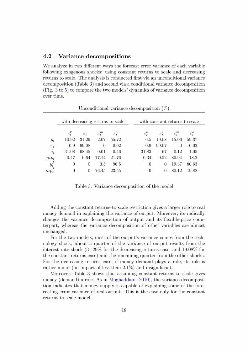
4.2 Variance decompositions
We analyze in two di¤erent ways the forecast error variance of each variablefollowing exogenous shocks: using constant returns to scale and decreasingreturns to scale. The analysis is conducted �rst via an unconditional variancedecomposition (Table 3) and second via a conditional variance decomposition(Fig. 3 to 5) to compare the two models� dynamics of variance decompositionover time.
Unconditional variance decomposition (%)
with decreasing returns to scale with constant returns to scale
"pt "it "mt "at "pt "it "mt "atyt 10.92 31.29 2.07 55.72 6.5 19.08 15.06 59.37
�t 0.9 99.08 0 0.02 0.9 99.07 0 0.02
it 31.08 68.45 0.01 0.46 31.83 67 0.12 1.05
mpt 0.47 0.64 77.14 21.76 0.34 0.52 80.94 18.2
yft 0 0 3.5 96.5 0 0 19.37 80.63
mpft 0 0 76.45 23.55 0 0 80.12 19.88
Table 3: Variance decomposition of the model
Adding the constant returns-to-scale restriction gives a larger role to realmoney demand in explaining the variance of output. Moreover, its radicallychanges the variance decomposition of output and its �exible-price coun-terpart, whereas the variance decomposition of other variables are almostunchanged.For the two models, most of the output�s variance comes from the tech-
nology shock, about a quarter of the variance of output results from theinterest rate shock (31.29% for the decreasing returns case, and 19.08% forthe constant returns case) and the remaining quarter from the other shocks.For the decreasing returns case, if money demand plays a role, its role israther minor (an impact of less than 2.1%) and insigni�cant.Moreover, Table 3 shows that assuming constant returns to scale gives
money (demand) a role. As in Moghaddam (2010), the variance decomposi-tion indicates that money supply is capable of explaining some of the fore-casting error variance of real output. This is the case only for the constantreturns to scale model.
18

As Table 3 shows, the money shock contribution to the business cycledepends on the returns to scale hypothesis.
0 10 20 30 40 50 600
20
40
60
80Decreasing Return to Scale
%
0 10 20 30 40 50 600
20
40
60
80Constant Return to Scale
Quarter
%
Preference ShockInterest Rate ShockMoney ShockProductivity Shock
Figure 3: Forecast error variance decomposition of output
If approximately half of the variance of output is still explained by the pro-ductivity shock, the role of the preference shock decreases notably, whereasthe impact of the interest rate shock increases over time. Figure 3 also con-�rms the signi�cant role of money (demand) in the dynamics of output, andits increasing role over periods, under the constant returns to scale hypoth-esis.A look at the conditional and unconditional in�ation variance decompo-
sitions shows the overwhelming role of the interest rate shock which explainsmore than 96% of the in�ation rate�s variance. As there is no signi�cantchange over the two models, we don�t represent this decomposition.
19

0 10 20 30 40 50 600
20
40
60
80
100Decreasing Return to Scale
%
0 10 20 30 40 50 600
20
40
60
80Constant Return to Scale
Quarter
%
Preference ShockInterest Rate ShockMoney ShockProductivity Shock
Figure 4: Forecast error variance decomposition of interest rate
The variance of the nominal interest rate is dominated by the direct shockto the interest rate. The relative importance of each of these shocks changesthrough time (Fig. 4). Over short horizons, the preference shock explainsalmost 70% of the nominal interest rate variance, whereas the interest rateshock explains less than 20%. For longer horizons, there is an inversion: thenominal interest rate shock explains close to 70% of the variance, and thepreference shock explains a bit more than 20%.Table 3 as well as the conditional variance decomposition of real money
balances shows that real money balances are mainly explained by the realmoney balances shock and the technology shock. As there is no signi�cantchange over the two models, we don�t represent this decomposition.
20
0 10 20 30 40 50 600
20
40
60
80
100Decreasing Return to Scale
%
0 10 20 30 40 50 600
20
40
60
80
100Constant Return to Scale
Quarter
%
Preference ShockInterest Rate ShockMoney ShockProductivity Shock
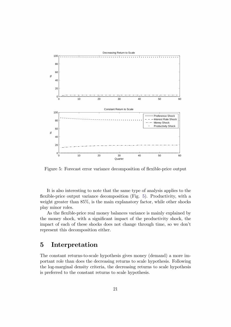
Figure 5: Forecast error variance decomposition of �exible-price output
It is also interesting to note that the same type of analysis applies to the�exible-price output variance decomposition (Fig. 5). Productivity, with aweight greater than 85%, is the main explanatory factor, while other shocksplay minor roles.As the �exible-price real money balances variance is mainly explained by
the money shock, with a signi�cant impact of the productivity shock, theimpact of each of these shocks does not change through time, so we don�trepresent this decomposition either.
5 Interpretation
The constant returns-to-scale hypothesis gives money (demand) a more im-portant role than does the decreasing returns to scale hypothesis. Followingthe log-marginal density criteria, the decreasing returns to scale hypothesisis preferred to the constant returns to scale hypothesis.
21

This result disproves the hypothesis of Short (1979), Startz (1984), Ben-zing (1989), and Chang (2002) of constant returns to scale for money in theproduction function and con�rms the hypothesis of Khan and Ahmad (1985)(decreasing returns).This criterion gives no signi�cant role to money (demand) in the dynamics
of the variables, despite its introduction in the production function.The simulation results are close to those obtained in the Galí (2008)
baseline model and provide interesting results about the potential e¤ect ofmoney on output and �exible-price output under the constant returns to scalehypothesis. Interestingly, and even if money enters the in�ation equation,the variance decomposition of in�ation with respect to shocks is una¤ectedunder the two hypotheses.
6 Conclusion
One of the most unsettled issues of the postwar economic literature involvesthe role of money as a factor of production. The notion of money as afactor of production has been debated both theoretically and empirically bya number of researchers in the past �ve decades. The question is whethermoney is an omitted variable in the production process.However, empirical support for money as an input along with labor (and
capital) has been mixed and, thus, the issue appears to be unsettled. Recentdevelopments involve a reexamination of the role of money (demand) in theproduction function. One of these development is the New Keynesian DSGEtheory mixed with Bayesian analysis.We depart from existing theoretical (and empirical) New Keynesian lit-
erature by building a New Keynesian DSGE model à la Galí (2008) thatincludes money in the production function, displaying money in the in�ationequation. Closing the model leads to the new concept of �exible-price realmoney balances.Despite their inclusion in the production function, and at least in the
unconstrained estimation, real money holdings do not play a signi�cant rolein the dynamics of the system. The only way to ascribe a role for real moneydemand in the dynamics of the system is to assume constant returns to scaleto factors of production, which is a strong and controversial hypothesis.Moreover, we con�rm that the model with decreasing returns to scale
is better than the model with constant returns to scale. Under decreasingreturns to scale, real money holdings do not play a signi�cant role in thedynamics of the economy. We also show that adding a money component tothe system does not necessarily create a role for it.
22

In this model, money demanded by households is also used (by them,as �rms� owners) as an input in production. But an issue of rival use (infacilitating transactions) would emerge. That is why for further research,as in Benhabib et al. (2001), a distinction between money for productiveand nonproductive use seems warranted. This perspective could enlarge ourmoney channel consideration.
7 Appendix
A Optimization problem
Our Lagrangian is given by
Lt = Et
"1X
k=0
CkUt+k � �t+kVt+k
#
where
Vt = Ct +Mt
Pt+Qt
BtPt�Bt�1Pt
�Wt
PtNt �
Mt�1
Pt
and
Ut = e"pt
C1��t
1� �+De"
mt
1� �
�Mt
Pt
�1����N1+�
t
1 + �
!
The �rst order condition related to consumption expenditures is given by
�t = e"ptC��t (32)
where �t is the Lagrangian multiplier associated with the budget constraintat time t.The �rst order condition corresponding to the demand for contingent
bonds implies that
�tQtPt= CEt
��t+1Pt+1
�(33)
The demand for cash that follows from the household�s optimization prob-lem is given by
De"pt e"
mt
�Mt
Pt
���= �t � CEt
��t+1
PtPt+1
�(34)
which can be naturally interpreted as a demand for real balances. The latteris increasing in consumption and is inversely related to the nominal interest
23

rate, as in conventional speci�cations.
�e"ptN�
t = �tWt
Pt(35)
We obtain from eq. (32)
�t = e"ptC
��
t , Uc;t = e"ptC
��
t (36)
where Uc;t =@Uk;t@Ct+k
CCCk=0. Eq. (36) de�nes the marginal utility of consumption.
Hence, the optimal consumption/savings, real money balances and laborsupply decisions are described by the following conditions:
F Combining (32) with (33) gives
Qt = CEt
"e"
pt+1C��t+1e"
ptC��t
PtPt+1
#, Qt = CEt
�Uc;t+1Uc;t
PtPt+1
�(37)
where Uc;t+1 =@Uk;t@Ct+k
CCCk=1. Eq. (37) is the usual Euler equation for
intertemporal consumption �ows. It establishes that the ratio of mar-ginal utility of future and current consumption is equal to the inverseof the real interest rate.
F Combining eq. (32) and eq. (34) gives
De"
mt
C��
t
�Mt
Pt
���= 1�Qt ,
Um;tUc;t
= 1�Qt (38)
where Um;t =@Uk;t
@(Mt+k=Pt+k)
CCCk=0. Eq. (38) is the intertemporal optimality
condition setting the marginal rate of substitution between money andconsumption equal to the opportunity cost of holding money.
F And combining eq. (32) and eq. (35) gives
�N�t
C��
t
=Wt
Pt,
Un;tUc;t
= �Wt
Pt(39)
where Un;t =@Uk;t@Nt+k
CCCk=0. Eq. (39) is the condition for the optimal
consumption-leisure arbitrage, implying that the marginal rate of sub-stitution between consumption and labor is equal to the real wage.
24

B Calibration
We estimate all parameters, except the discount factor (C), the inverse ofthe Frisch elasticity of labor supply (�), and the elasticity of demand ofhouseholds for consumption goods (").Following standard conventions, we calibrate beta distributions for pa-
rameters that fall between zero and one, inverted gamma distributions forparameters that need to be constrained to be greater than zero and normaldistributions in other cases.As our goal is to compare two models, we adopt the same priors in the two
models with the same calibration, except for the return to scale parameter.The calibration of � is inspired by Rabanal and Rubio-Ramírez (2005) andCasares (2007). They choose, respectively, a risk aversion parameter of 2:5and 1:5. In line with these values, we consider that � = 2 corresponds to astandard risk aversion, as in Benchimol and Fourçans (2012).As in Smets and Wouters (2003), the standard errors of the innovations
are assumed to follow inverse gamma distributions, and we choose a betadistribution for shock persistence parameters (as well as for the backwardcomponent of the Taylor rule, scale parameters, D and �, price stickinessindex, �, and output elasticities of labor, Bn, and of real money balances,Bm, of the production function) that should be lesser than one.The calibration of B, C, �, � and " comes from Casares (2007) and Galí
(2008). The smoothed Taylor rule (�i, ��, and �x) is calibrated followingGerlach-Kristen (2003), with priors analogous to those used by Smets andWouters (2003). In order to take into consideration possible behaviors of thecentral bank, we assign a higher standard error for the Taylor rule coe¢cients.All the standard errors of shocks are assumed to be distributed according
to inverted Gamma distributions, with prior means of 0.02. The latter lawensures that these parameters have a positive support. The autoregressiveparameters are all assumed to follow Beta distributions. All these distribu-tions are centered around 0.75 and we take a common standard error of 0.1for the shock persistence parameters, as in Smets and Wouters (2003).
25

C Priors and posteriors
C.1 Model with decreasing returns to scale
0.02 0.04 0.06 0.08 0.10
200
400
600
800
SE_ua
0.02 0.04 0.06 0.08 0.10
200
400
SE_ui
0.05 0.1 0.15 0.20
20
40
60
SE_up
0.02 0.04 0.06 0.08 0.10
100
200
SE_um
0.2 0.4 0.6 0.8 10
2
4
6
8
alphan
0 0.2 0.4 0.6 0.80
5
10
15
alpham
0.5 0.6 0.7 0.8 0.90
5
10
15
teta
1.5 2 2.50
1
2
3
4
nu
1.5 2 2.50
1
2
3
4
sigma
- 0.2 0 0.2 0.4 0.6 0.80
1
2
3
4
gamma
- 0.2 0 0.2 0.4 0.6 0.80
1
2
3
4
khi
0.2 0.4 0.6 0.80
2
4
6
8
li1
2 3 40
0.5
1
1.5
2
li2
1 2 30
0.5
1
1.5
2
li3
0.4 0.6 0.8 10
5
10
15
rhoa
0.4 0.6 0.8 10
10
20
30rhop
0.4 0.6 0.8 10
50
100
rhoi
0.4 0.6 0.8 10
5
10
15
20
rhom
0.4 0.6 0.8 10
10
20
30
rhop
0.4 0.6 0.8 10
50
100
rhoi
0.4 0.6 0.8 10
10
20
rhom
26

C.2 Model with constant returns to scale
0.02 0.04 0.06 0.08 0.10
200
400
600
SE_ua
0.02 0.04 0.06 0.08 0.10
200
400
SE_ui
0.05 0.1 0.15 0.20
20
40
60
SE_up
0.02 0.04 0.06 0.08 0.10
100
200
SE_um
0.2 0.4 0.6 0.80
5
10
alphan
0.5 0.6 0.7 0.8 0.90
5
10
15
teta
1.8 2 2.2 2.4 2.6 2.80
1
2
3
4
nu
1.5 2 2.50
1
2
3
4
sigma
- 0.2 0 0.2 0.4 0.6 0.80
1
2
3
4
gamma
0 0.5 10
1
2
3
4
khi
0.2 0.4 0.6 0.80
2
4
6
8
li1
2 3 40
0.5
1
1.5
2
li2
1 2 30
0.5
1
1.5
2
li3
0.4 0.6 0.8 10
5
10
15
rhoa
0.4 0.6 0.8 10
10
20
rhop
0.4 0.6 0.8 10
50
100
rhoi
0.4 0.6 0.8 10
10
20
rhom
27

D Robustness checks
Each graph represents speci�c convergence measures with two distinct linesthat show the results within (red line) and between (blue line) chains (Geweke,1999). Those measures are related to the analysis of the model parametersmean (interval), variance (m2) and third moment (m3). For each of the threemeasures, convergence requires that both lines become relatively horizontaland converge to each other in both models4.
D.1 Model with decreasing returns to scale
1 2 3 4 5 6 7 8 9 10
x 104
6
6.5
7
7.5
8Interval
1 2 3 4 5 6 7 8 9 10
x 104
4
6
8
10m2
1 2 3 4 5 6 7 8 9 10
x 104
20
30
40
50m3
4Robustness analysis with respect to calibrated parameters is available upon request.
28

D.2 Model with constant returns to scale
1 2 3 4 5 6 7 8 9 10
x 104
7
7.5
8
8.5Interval
1 2 3 4 5 6 7 8 9 10
x 104
7
8
9
10m2
1 2 3 4 5 6 7 8 9 10
x 104
30
40
50
60m3
E Macro parameters
Decreasing Constant
returns to scale returns to scale
�ya 1.026665 1.048629
�ym -0.116906 0.379180
�yc -0.085881 0.221747
�my+1 -0.496467 -0.443291
�my 0.866771 0.773933
�mc 0.167187 0.1578931�
0.467391 0.434287
�x 0.047323 0.047126
�m 0.005532 -0.017869
��1 0.539232 0.561143
�c -0.010050 -0.010050��
0.866771 0.773933a2�
0.164496 0.155393�m�
0.467391 0.434287
�� (1� �i) 1.681117 1.461802
�x (1� �i) 0.948134 0.806101
�i 0.475001 0.543219
29

References
Adolfson, M., Laseen, S., Linde, J., Villani, M., 2007. Bayesian estimation ofan open economy DSGE model with incomplete pass-through. Journalof International Economics 72 (2), 481-511.
Adolfson, M., Laseen, S., Linde, J., Villani, M., 2008. Evaluating an esti-mated new Keynesian small open economy model. Journal of EconomicDynamics and Control 32 (8), 2690-2721.
Ben-Zion, U., and Ruttan, V.W., 1975. Money in the production function:an interpretation of empirical results. The Review of Economics andStatistics 57(2), 246-247.
Benchimol, J., and Fourçans, A., 2012. Money and risk in a DSGE frame-work: a Bayesian application to the Eurozone. Journal of Macroeco-nomics 34(1), 95-111.
Benhabib, J., Schmitt-Grohé, S., and Uribe, M., 2001. Monetary policy andmultiple equilibria. American Economic Review 91(1), 167-186.
Benzing, C., 1989. An update on money in the production function. EasternEconomic Journal 15(3), 235-239.
Calvo, G.A., 1983. Staggered prices in a utility-maximizing framework. Jour-nal of Monetary Economics 12(3), 383-398.
Casares, M., 2007. Monetary policy rules in a new Keynesian Euro areamodel. Journal of Money, Credit and Banking 39 (4), 875-900.
Chang, W., 2002. Examining the long-run e¤ect of money on economicgrowth: an alternative view. Journal of Macroeconomics 24(1), 81-102.
Clarida, R., Galí, J., and Gertler, M., 1999. The science of monetary policy: anew Keynesian perspective. Journal of Economic Literature 37(4), 1661-1707.
Cobb, C.W., and Douglas, P.H., 1928. A theory of production. AmericanEconomic Review 18(1), 139-165.
Christiano, L., Eichenbaum, M., Evans, C., 1997. Sticky price and limitedparticipation models of money: a comparison. European Economic Re-view 41(6), 1201-1249.
30

Fagan, G., Henry, J., Mestre, R., 2001. An Area-Wide Model (AWM) for theEuro area. European Central Bank Working Paper No. 42.
Fischer, S., 1974. Money and the production function. Economic Inquiry12(4), 517-33.
Friedman, M., 1959. The demand for money: some theoretical and empiricalresults. Journal of Political Economy 64(1), 327-351.
Friedman, M., 1969. The optimum quantity of money and other essays.Chicago: Aldine Publishing Co.
Galí, J., 2008. Monetary policy, in�ation and the business cycle: an intro-duction to the new Keynesian framework. Princeton University Press,Princeton, NJ.
Gerlach-Kristen, P., 2003. Interest rate reaction functions and the Taylor rulein the Euro area. European Central Bank Working Paper No. 258.
Geweke, J., 1999. Using simulation methods for Bayesian econometric mod-els: inference, development, and communication. Econometric Reviews18 (1), 1-73.
Hasan, M.A., and Mahmud, S.F., 1993. Is money an omitted variable in theproduction function ? Some further results. Empirical Economics 18(3),431-445.
Ireland, P.N., 2004. Money�s role in the monetary business cycle. Journal ofMoney, Credit and Banking 36(6), 969-983.
Jeanne, O., 1994. Nominal rigidities and the liquidity e¤ect. Mimeo ENPC-CERAS.
Johnson, H.G., 1969. Inside money, outside money, income, wealth and wel-fare in monetary theory. Journal of Money Credit and Banking 1(1),30-45.
Khan, A.H., and Ahmad, M., 1985. Real money balances in the productionfunction of a developing country. The Review of Economics and Statistics67(2), 336-340.
Levhari, D., and Patinkin, D., 1968. The role of money in a simple growthmodel. American Economic Review 58(4), 713-753.
31

Moghaddam, M., 2010. Co-integrated money in the production function-evidence and implications. Applied Economics 42(8), 957-963.
Rabanal, P., Rubio-Ramírez, J.F., 2005. Comparing new Keynesian models ofthe business cycle: a Bayesian approach. Journal of Monetary Economics52(6), 1151-1166.
Sephton, P.S., 1988. Money in the production function revisited. AppliedEconomics 20(7), 853-860.
Short, E.D., 1979. A new look at real money balances as a variable in theproduction function. Journal of Money, Credit and Banking 11(3), 326-339.
Sinai, A., and Stokes, H.H., 1972. Real money balances: an omitted variablefrom the production function ?. The Review of Economics and Statistics54(3), 290-296.
Sinai, A., and Stokes, H.H., 1975. Real money balances: an omitted variablefrom the production function ? A reply. The Review of Economics andStatistics 57(2), 247-252.
Sinai, A., and Stokes, H.H., 1977. Real money balances as a variable in theproduction function: reply. Journal of Money, Credit and Banking 9(2),372-373.
Sinai, A., and Stokes, H.H., 1981. Real money balances in the productionfunction: a comment. Eastern Economic Journal 17(4), 533-535.
Sinai, A., and Stokes, H.H., 1989. Money balances in the production function:a retrospective look. Eastern Economic Journal 15(4), 349-363.
Smets, F., and Wouters, R., 2003. An estimated Dynamic Stochastic GeneralEquilibrium model of the Euro area. Journal of the European EconomicAssociation 1(5), 1123-1175.
Smets, F., Wouters, R., 2007. Shocks and frictions in US business cycles: aBayesian DSGE approach. American Economic Review 97 (3), 586 -606.
Startz, R., 1984. Can money matter ?. Journal of Monetary Economics 13(3),381-385.
Stein, J.L., 1970. Monetary growth theory in perspective. American Eco-nomic Review 60(1), 85-106.
32

Subrahmanyam, G., 1980. Real money balances as a factor of production:some new evidence. The Review of Economics and Statistics 62(2), 280-283.
Walsh, C.E., 2010. Monetary theory and policy. The MIT Press, Cambridge,MA.
Woodford, M., 2003. Interest and prices: foundations of a theory of monetarypolicy. Princeton University Press, Princeton, NJ.
You, J.S., 1981. Money, technology, and the production function: an empir-ical study. The Canadian Journal of Economics 14(3), 515-524.
33