External Shocks, Banks and Optimal Monetary Policy: A Recipe

for Emerging Market Central Banks1

Yasin Mimir2 Enes Sunel3

September 28, 2017

Abstract

We document that the 2007-09 Global Financial Crisis exposed emerging market economiesto an adverse feedback loop of capital outflows, depreciating exchange rates, deterioratingbalance sheets, rising credit spreads and falling real economic activity. We account for theseempirical findings, by building a New-Keynesian DSGE model of a small open economywith a banking sector that has access to both domestic and foreign funding. Using thecalibrated model, we investigate optimal, simple and implementable monetary policy rulesthat respond to domestic/external financial variables alongside inflation and output. TheRamsey-optimal policy rule is used as a benchmark. The results suggest that such rulesfeature direct and non-negligible responses to the real exchange rate, asset prices andlending spreads. Furthermore, interest rate policy takes a stronger anti-inflationary stancewhen financial stability considerations are addressed by the monetary policy. We find thata countercyclical reserve requirement rule which responds to fluctuations in credit spreadsand is optimized jointly with a conventional interest rate rule dominates augmented Taylorrules under country risk premium shocks.

Keywords: Optimal monetary policy, banks, credit frictions, external shocks, foreign debt.JEL Classification: E44, E52, F41

1We would like to thank Leonardo Gambacorta, Nobuhiro Kiyotaki, Giovanni Lombardo, Hyun Song Shin, PhilipTurner, the seminar participants at the Bank for International Settlements, the Central Bank of Turkey, NorgesBank, the Georgetown Center for Economic Research Biennial Conference 2015, the CBRT-BOE Joint Workshop2015 on “The International Monetary and Financial System – long-term challenges, short-term solutions”, the 21stInternational Conference on Computing in Economics and Finance, the 11th World Congress of the EconometricSociety, and the 47th Money, Macro and Finance Research Group Annual conference for their helpful comments andsuggestions. This paper circulated earlier under the title “External Shocks, Banks and Optimal Monetary Policy in anOpen Economy”. Yasin Mimir completed this project while visiting the Bank for International Settlements under theCentral Bank Research Fellowship programme. The views expressed in this paper are those of the authors only anddo not necessarily reflect the views of Norges Bank or of the Bank for International Settlements (BIS). The usualdisclaimer applies.

2Corresponding author. Norges Bank, Monetary Policy Department, Bankplassen 2, 0151 Oslo, Norway, Phone:+4722316811, yasin.mimir@norges-bank.no, Personal homepage: http://www.yasinmimir.com

3Sunel & Sunel Law Firm. Soganlik Yeni Mah., Uprise Elite Residence 234, Kartal, 34880 Istanbul, Turkey, Phone:+905334451145, email: enessunel@gmail.com, Personal homepage: https://sites.google.com/site/enessunel/

i

1 Introduction

The 2007-09 Global Financial Crisis exposed emerging market economies (EMEs) to an adverse

feedback loop of capital outflows, depreciating exchange rates, deteriorating balance sheets, rising

credit spreads and falling real economic activity. Furthermore, the unconventional response of

advanced economy policymakers to the crisis caused EMEs to sail in uncharted waters from a

monetary policymaking perspective. These adverse developments revitalized the previous debate

about whether central banks should pay attention to domestic or external financial variables over and

above their effects on inflation or real economic activity. Consequently, the lean-against-the-wind

(LATW) policies - defined as augmented Taylor-type monetary policy rules that additionally respond

to domestic or external financial variables - are now central to discussions in both academic and

policy circles.1 This debate is even more pronounced in EMEs in which banks are the main source

of credit extension and their sizeable reliance on non-core debt amplifies the transmission of external

shocks, threatening both price and financial stability objectives.2 In this regard, this paper aims to

provide a recipe for EME central banks in rethinking interest rate policy determination.

We study optimal monetary policy in an open economy with financial market imperfections in

the presence of both domestic and external shocks. Using a canonical New-Keynesian DSGE model

of a small open economy augmented by a banking sector that has access to both domestic and foreign

funds, we investigate the quantitative performances of optimal, simple and implementable LATW-

type interest rate rules relative to a Ramsey-optimal monetary policy rule. We follow the definition

of Schmitt-Grohe and Uribe (2007) in constructing such rules that respond to easily observable

macroeconomic variables while preserving the determinacy of equilibrium. We consider a small

number of targets among a wide range of variables that are arguably important for policymaking. In

particular, we look at the level of bank credit, asset prices, credit spreads, the U.S. interest rate and

the real exchange rate as additional inputs to policy. We then compare these optimal LATW-type

Taylor rules with standard optimized Taylor rules (with and without interest-rate smoothing).

Our model builds on Galı and Monacelli (2005). The main departure from their work is that

we introduce an active banking sector as in Gertler and Kiyotaki (2011). In this class of models,

financial frictions require banks to collect funds from external sources while limiting their demand

for debt because of an endogenous leverage constraint resulting from a costly enforcement problem.

This departure generates a financial accelerator mechanism by which the balance sheet fluctuations

of banks affect real economic activity. Our model differs from that of Gertler and Kiyotaki (2011) in

that it replaces interbank borrowing by foreign debt in an open economy setup. Consequently, the

endogenous leverage constraint of bankers is additionally affected by fluctuations in the exchange

rate.

1See the discussion in Angelini et al. (2011).2The median share of bank credit in total credit to the non-financial sector in EMEs was 87% in 2013 while the

median share of non-core debt in total liabilities was 33%. For more details, see Ehlers and Vıllar (2015). For otherrelated discussions, see Obstfeld (2015) and Rey (2015).

1

We assume that frictions between banks, on one side, and their domestic and foreign creditors,

on the other side, are asymmetric. Specifically, domestic depositors are assumed to be more efficient

than international investors in recovering assets from banks in case of bankruptcy. This makes

foreign debt more risky, creates a wedge between the real costs of domestic and foreign debt, and

hence violates the uncovered interest parity (UIP) condition.3 This key ingredient gives us the

ability to empirically match the liability structure of domestic banks (which is defined as the share

of non-core liabilities in total bank liabilities) and analyze changes in this measure in response

to external shocks. Lastly, our model incorporates various real rigidities that generally form part

of medium-scale DSGE models such as those studied by Christiano et al. (2005) and Smets and

Wouters (2007). In particular, the model’s empirical fit is improved by features such as habit

formation in consumption, variable capacity utilization and investment adjustment costs.

First, we analytically derive the intratemporal and intertemporal wedges in our model economy

and compare them to a first-best flexible-price closed economy model to better understand the policy

trade-offs that the Ramsey planner faces in response to shocks. We show that the distortions in the

intratemporal wedge are mainly driven by the variations in the inflation rate and the real exchange

rate induced by monopolistic competition, price stickiness, home bias and incomplete exchange rate

pass-through. At the same time, the distortions in the intertemporal wedge are mainly driven by the

variations in the lending spreads over the costs of domestic and foreign deposits together with those

in the real exchange rate induced by financial market imperfections and open economy features.

We then conduct our quantitative analysis under five different types of shocks that might be most

relevant for optimal policy prescription in EMEs. The first two of these are total factor productivity

and government spending, which we label as domestic shocks. The remaining three are the country

borrowing premium, the U.S. interest rate and export demand, which we label as external shocks.4

Finally, we also analyze optimal policy in an economy driven jointly by all of these shocks given

that it might be difficult for the monetary authority to perfectly disentangle the different sources of

business cycle movements while designing its policy.

We find that the Ramsey-optimal policy substantially reduces relative volatilities of inflation,

markup, the real exchange rate and loan-deposits interest rate spreads, compared to a decentralized

economy, in which interest rate policy is a standard Taylor rule calibrated to the data. Morevoer,

in comparison with the optimized simple rules, the Ramsey-optimal policy produces fairly smaller

degrees of volatility in inflation and the real exchange rate while implying relatively larger degrees of

volatility in credit spreads and asset prices. High volatility in credit spreads hints that the Ramsey

planner weighs distortions resulting from price dispersion and exchange rate fluctuations more,

3We empirically illustrate in the bottom-left panel of Figure 1 that, with the exception of the period 2010:Q2-2011:Q3, credit spreads on foreign debt are larger than credit spreads on domestic deposits. This implies that domesticdeposit rates are higher than foreign deposit rates. This regularity dates back to 2002:Q4 for the average EME in oursample. For a detailed survey on the violation of the UIP, see Engel (2015). For theoretical contributions on domesticfunding premium, see Broner et al. (2014) and Fornaro (2015).

4A shock to a country’s borrowing premium can be justified by the reduction in the global risk appetite driven bythe collapse of Lehman Brothers in September 2008 or the taper tantrum of May 2013. A shock to the U.S. interestrate can be justified by the accommodative monetary stance of the Federal Reserve in the aftermath of the crisis orthe policy normalization that was expected in late 2015.

2

compared with stabilizing inefficiencies resulting from credit frictions. Increased volatility in asset

prices on the other hand, relates to the mechanism discussed by Faia and Monacelli (2007) that the

constrained planner is adjusting asset prices to bring fluctuations in investment closer to efficient

fluctuations. This is mainly because asset prices effectively work as a procyclical tax on investment

under adjustment costs. The rationale behind this is similar to that in Arseneau and Chugh (2012)

in which the Ramsey planner increases the volatility of labor income tax rate under labor market

frictions to bring fluctuations in employment closer to the efficient fluctuations.

Under country risk premium shocks, the real exchange rate (RER) augmented rule which displays

an aggressive and positive response to fluctuations in the real exchange rate and only mild responses

to inflation and output variations implies the largest welfare among all optimized augmented Taylor

rules. The implied welfare loss of this policy vis-a-vis the Ramsey-optimal policy is 0.0015% in terms

of changes that compensate variation in consumption. This suggests that addressing the financial

channel for an EME central bank is crucial (by which exchange rate depreciation hurts the balance

sheets of domestic borrowers who face currency mismatch, leading them to curb domestic demand)

rather than leaving adjustments to the trade channel that operates via price competitiveness as

empirically documented by Kearns and Patel (2016). Since central bank is already fighting the

pass-through aggressively, it does not deem useful to take a strong anti-inflationary stance under

this policy. This finding is linked to the insights discussed by Monacelli (2005) and Monacelli (2013)

that under incomplete exchange rate pass-through, fluctuations in the exchange rate operate as

endogenous cost-push shocks which optimal policy pays more attention relative to price stability

concerns.

Our results confirm the findings of Faia and Monacelli (2007) that an easing in the policy rate

gets the dynamics of investment closer to efficient fluctuations in response to a favorable shock. To

that end, we find that optimal policy calls for a negative response to asset prices together with a

moderate anti-inflationary stance. The welfare cost implied by this policy rule is 0.0021% against

the Ramsey policy. We find that the credit spread-augmented Taylor rule achieves a level of welfare

very close to that of the asset price-augmented Taylor rule (the implied cost is 0.0026%). Interest

rate policy features a LATW role in this case because credit spreads are countercyclical and the

optimized augmented rule calls for an easing in bad times.

An optimized standard Taylor rule calls for a much milder anti-inflationary stance than those

obtained under either the asset price- or the credit spread-augmented rules and is welfare inferior.

The reason why standard Taylor rules perform suboptimally hinges on the idea that in response to

adverse external shocks (which already raise the cost of foreign debt), a strong anti-inflationary

stance of interest rate policy would hurt bank balance sheets even more by increasing the cost of

domestic deposits. Therefore, we show that using an augmented policy rule with financial stability

considerations allows the central bank to take a stronger anti-inflationary stance in line with the

insights of Aoki et al. (2016).

When all shocks are switched on, we find that the asset-price augmented rule achieves the highest

welfare among alternative optimal simple rules. The welfare cost of implementing this policy relative

3

to the Ramsey-optimal policy rule is 0.0013%. Our findings are broadly in line with the case of

external shocks that responding to credit spreads or the exchange rate is welfare superior compared

to implementing an optimal standard Taylor rule. We also consider monetary policy responses to

the U.S. interest rates motivated by the idea that domestic policy rates in EMEs might partly be

driven by changes in the U.S. interest rates over and above what domestic factors would imply.

The model suggests that it is optimal to positively respond to the U.S. interest rates in line with

the empirical findings and discussions of Takats and Vela (2014) and Hofmann and Takats (2015).

Although this policy rule dominates an optimal standard Taylor rule, it produces a larger welfare

cost than those implied by the RER-, asset price- or credit spread-augmented interest rate policies.

Using the short-term interest rate for LATW purposes might be difficult should hitting multiple

stabilization goals necessitate different trajectories for the single policy tool. In this respect, Shin

(2013) and Chung et al. (2014) emphasize the usefulness of liability-based macroprudential policy

tools alongside conventional monetary policy. To contemplate on those issues, we operationalize

reserve requirements as a policy rule that aims to smooth out fluctuations in credit spreads in

addition to conventional interest rate policy. We then examine whether an optimized mix of these

two tools can compete with an optimized augmented interest rate rule in maximizing household

welfare. We find that optimal reserve requirement policy exhibits LATW as it features a negative

response to credit spreads. In addition, such a policy mix is found to produce welfare costs that

are even smaller than that implied by the RER-augmented interest rate policy under country risk

premium shocks.

Related literature

This paper is related to a vast body of literature on the optimality of responses to financial

variables. In closed-economy frameworks, Faia and Monacelli (2007) use a New-Keynesian model

with agency costs to argue that responding negatively to asset prices with a Taylor-type interest

rate rule is welfare improving. Curdia and Woodford (2010) find that it is optimal to respond to

credit spreads under financial disturbances in a model with costly financial intermediation. Gilchrist

and Zakrajsek (2011) show that a spread-augmented Taylor rule smooths fluctuations in real and

financial variables in the Bernanke et al. (1999) model. Hirakata et al. (2013), and Gambacorta and

Signoretti (2014) consider frameworks with an explicit and simultaneous modeling of non-financial

firms and banks balance sheets. The former study shows that a spread-augmented Taylor rule

stabilizes the adverse effects of shocks that widen credit spreads while the latter paper shows that

responding to asset prices entails stabilization benefits even in response to supply side shocks.

Notarpietro and Siviero (2015) investigate whether it is welfare-improving to respond to house price

movements using the Iacoviello and Neri (2010) model with housing assets and collateral constraints.

Angeloni and Faia (2013) suggest that smoothing movements in asset prices in conjunction with

capital requirements is welfare improving relative to simple policy rules in a New-Keynesian model

with risky banks. Angelini et al. (2011) show that macroprudential policy instruments, such as

4

capital requirements and loan-to-value ratios, are effective in response to financial shocks. Mimir et

al. (2013) illustrate that countercyclical reserve requirements that respond to credit growth have

desirable stabilization properties. We differ from these papers by considering the Ramsey-optimal

policy rule and investigating optimal, simple and implementable interest rate rules that augment

domestic or external financial variables in an open economy framework.

Glocker and Towbin (2012) investigate the interaction of alternative monetary policy rules

and reserve requirements within a model of financial accelerator in which firms borrow either only

from domestic depositors or foreign investors. Medina and Roldos (2014) focus on the effects of

alternative parameterized monetary and macroprudential policy rules in an open economy with a

modeling of the financial sector that is different from ours. They find that the LATW capabilities

of conventional monetary policy might be limited. Akinci and Queralto (2014) consider occasionally

binding leverage constraints faced by banks that can also issue new equity within a small open

economy model. They show that macroprudential taxes and subsidies are effective in lowering the

probability of financial crises and increase welfare. However, they abstract from nominal rigidities

and the role of monetary policy in relation to financial stability in EMEs. Kolasa and Lombardo

(2014) study optimal monetary policy in a two-country DSGE model of the euro area with financial

frictions as in Bernanke et al. (1999), and under which firms can collect both domestic and foreign

currency-denominated debt. They find that the monetary authority should correct credit market

distortions at the expense of deviations from price stability.

In a closely related paper, Aoki et al. (2016) consider monetary and financial policies in EMEs

using a small open economy New Keynesian setup with banks that are subject to currency risk.

They model financial policies as net worth subsidies, which are financed by taxes on risky assets or

foreign currency borrowing and show that there are significant gains from combining such measures

with monetary policy. Our paper generalizes their finding that from a welfare maximizing point of

view; interest rate policy displays a stronger anti-inflationary stance when either it is augmented

with a financial stabilization objective or accompanied by an additional financial stabilization tool

such as reserve requirements. This finding hinges on the property that all else equal, stronger

anti-inflationary stance of interest rate policy hurts bank balance sheets as it increases the cost of

funds for banks. Our paper differs from the work of Aoki et al. (2016) in three main ways. First, we

model asymmetric financial frictions between domestic and foreign borrowing of banks differently.

Second, and most importantly, our paper analyzes optimal Ramsey policy and optimized augmented

interest rate rules rather than comparing parameterized alternative policy rules. Third, financial

policies in our paper include LATW-type Taylor rules and reserve requirements instead of taxes on

foreign debt or risky assets.

Under certain cases, optimal interest rate policy in our work calls for a positive response to

exchange rate depreciations. This places our paper within the strand of literature surveyed by

Engel (2014) which makes a case for targeting currency mismatches in order to ease financial

conditions faced by borrowers (in our case banks). Finally, our analysis also sheds light on the

5

discussions regarding the monetary trilemma and the associated challenges that the EME monetary

policymakers face as discussed by Obstfeld (2015) and Rey (2015).

This paper contributes to the literature surveyed above in four main respects. First, in a small

open economy setup, we investigate the optimality of responding to developments in domestic

financial conditions as well as fluctuations in the exchange rate that are linked to capital flows

which are highly relevant for EMEs. Second, we study the role of a banking sector which can

raise both domestic and foreign funds in the transmission of augmented interest rate and reserve

requirements policies. Third, we derive analytically the intratemporal and intertemporal wedges

in the model economy, and characterize the optimal monetary policy rule by solving the Ramsey

planner’s problem. Finally, we construct optimal and simple augmented interest rate policy rules

as well as an optimal policy mix of a conventional Taylor rule and a macroprudential reserve

requirements policy.

The rest of the paper is structured as follows. Section 2 provides a systematic documentation

of the adverse feedback loop faced by EMEs during the Global Financial Crisis. In Section 3, we

describe our theoretical framework. Section 4 focuses on our quantitative analysis and investigates

optimal, simple and implementable monetary policy rules for EMEs. Finally, Section 5 concludes.

2 The 2007-09 crisis and macroeconomic dynamics in the EMEs

Although the crisis originated in advanced economies, EMEs experienced the severe contractionary

effects induced by it as Figure 1 clearly illustrates for 20 EMEs around the 2007-09 episode. In

the figure, variables regarding the real economic activity and the external side are depicted by

cross-country simple means of deviations from HP trends.5 The top-left panel of the figure illustrates

that the sharp reversal of capital inflows to EMEs is accompanied by a roughly 400 basis points

increase in the country borrowing premiums (the top-middle panel), as measured by the EMBI

Global spread, leading to sharp hikes in lending spreads over the costs of domestic and foreign funds

by around 400 basis points (the bottom-left panel). Finally, the cyclical components of the real

effective exchange rate and current account-to-GDP ratio (illustrated in the bottom-middle panel)

displayed a depreciation and a reversal of about 10% and 2%, respectively. In addition to these facts,

Mihaljek (2011) documents that the tightening in domestic financial conditions in EMEs coincides

with substantial declines in domestic deposits and disproportionately more reduction in foreign

borrowing of banks which resulted in dramatic falls in their loans to corporations. As a result of

these adverse developments in domestic and external financial conditions, GDP and consumption

declined by around 4% and investment fell by 8% compared to their HP trend levels in EMEs.

We also illustrate cross-sectional developments in the EME group by providing Table 1, which

displays the peak-to-trough changes in macroeconomic and financial variables in the 2007:Q1-

5Data sources used in this section are the Bank for International Settlements, Bloomberg, EPFR, InternationalMonetary Fund and individual country central banks. Countries included in the analysis are Brazil, Chile, China,Colombia, Czech Republic, Hungary, India, Indonesia, Israel, Korea, Malaysia, Mexico, Peru, Philippines, Poland,Russia, Singapore, South Africa, Thailand, and Turkey. Using medians of deviations for the plotted variables producesimilar patterns.

6

2011:Q3 episode for each individual EME in our sample. The average changes in variables might

be different than those plotted in Figure 1 since the exact timing of peak-to-trough is different for

each EME. The table indicates that there is a substantial heterogeneity among EMEs in terms

of the realized severity of the financial crisis. With the intention of mitigating the crisis, EME

central banks first raised policy rates to curb accelerating capital outflows in the initial phase, and

then gradually eased their policy stances (of about 4 percentage points in 6 quarters) thanks to

the accommodative policies of advanced economies during the crisis. Reserve requirements, on the

other hand, complemented conventional monetary policy at the onset of the crisis and appear to

substitute it when there was a sharp upward reversal in capital flows in the aftermath of the crisis.6

All in all, it is plausible to argue that the 2007-09 global financial crisis exposed EMEs to an

adverse feedback loop of capital outflows, depreciating exchange rates, deteriorating balance sheets,

rising credit spreads and falling real economic activity. The policy response of authorities in these

countries on the other hand, is strongly affected by the repercussions of the unconventional policy

measures introduced by advanced economies and displayed diversity in the set of policy tools used.

The next section provides a theory that replicates these features of the data and explores what kind

of monetary policy design could be deemed as optimal from a welfare point of view.

3 Model economy

The analytical framework is a medium-scale New Keynesian small open economy model inhabited

by households, non-financial firms, capital producers, and a government. There is a single tradable

consumption good which is both produced at home and imported (exported) from (to) the rest of

the world. Intermediate goods producers use capital and labor and determine the nominal price

of their good in a monopolistically competitive market subject to menu costs as in Rotemberg

(1982). Final goods producers on the other hand, repackage the domestically produced and imported

intermediate goods in a competitive market in which the prices of aggregated home and foreign

goods are determined. Home goods are consumed by workers and capital goods producers, and are

exported to the rest of the world. Similarly, foreign goods are consumed by workers and are used by

capital goods producers.

Households are composed of worker and banker members who pool their consumption together.

Workers earn wages and profit income, save in domestic currency denominated, risk-free bank

deposits and derive utility from consumption, leisure and holding money balances. Different from

standard open economy models, we assume that workers do not trade international financial assets,

since banker members of households carry out the balance of payments operations of this economy

by borrowing from abroad.

Intermediate goods producers cannot access to household savings and instead finance their

capital expenditures by selling equity claims to bankers. After financing their capital expenditures,

6The abrupt decline of about 4 percentage points in reserve requirements from 2009:Q4 to 2010:Q1 is mostly dueto Colombia and Peru as they reduced their reserve requirement ratios by 16 and 9 percentage points, respectively.

7

they buy capital from capital producers who use home and foreign investment goods as inputs,

repair the worn out capital and produce new capital.

Financial frictions define bankers as the key agents in the economy. The modeling of the banking

sector follows Gertler and Kiyotaki (2011), with the modification that bankers make external

financing from both domestic depositors and international investors, potentially bearing currency

risk. With their debt and equity, bankers fund their assets that come in the form of firm securities.

Finally, the consolidated government makes an exogeneous stream of spending and determines

short-term interest rate as well as reserve requirements policy.

The benchmark monetary policy regime is a Taylor rule that aims to stabilize inflation and

output. In order to understand the effectiveness of alternative monetary policy rules, we augment

the baseline policy framework with a number of various domestic or external financial stability

objectives. In addition, we analyze the use of reserve requirements that countercyclically respond to

credit spreads over the cost of non-core bank borrowing. Unless otherwise stated, variables denoted

by upper (lower) case letters represent nominal (real) values in domestic currency. Variables that

are denominated in foreign currency or related to the rest of the world are indicated by an asterisk.

For brevity, we include key model equations in the main text. Interested readers might refer to

Online Appendix A for detailed descriptions of the optimization problems of workers, firms, capital

producers and bankers as well as the definition of the competitive equilibrium.

3.1 Prices

The nominal exchange rate of the foreign currency in domestic currency units is denoted by

St. Therefore, the real exchange rate of the foreign currency in terms of real home goods becomes

st =StP ∗tPt

, where foreign currency denominated CPI, P ∗t , is taken exogenously. We assume that

foreign goods are produced in a symmetric setup as in home goods. That is, there is a continuum of

foreign intermediate goods that are bundled into a composite foreign good, whose consumption by

the home country is denoted by cFt . We assume that the law of one price holds for the import prices of

intermediate goods, that is, MCFt = StPF∗t , where MCFt is the marginal cost for intermediate good

importers and PF∗t is the foreign currency denominated price of such goods. Foreign intermediate

goods producers charge a markup over the marginal cost MCFt while setting the domestic currency

denominated price of foreign goods. The small open economy also takes PF∗t as given. In Online

Appendix A.5, we elaborate further on the determination of the domestic currency denominated

prices of home and foreign goods, PHt and PFt .

3.2 Banks

The modeling of banks closely follows Gertler and Kiyotaki (2011) except that banks in our

model borrow in local currency from domestic households and in foreign currency from international

lenders. They combine these funds with their net worth, and finance capital expenditures of home-

based tradable goods producers. For tractability, we assume that banks only lend to home-based

production units.

8

The main financial friction in this economy originates from a moral hazard problem between

bankers and their funders, leading to an endogenous borrowing constraint on the former. The agency

problem is such that depositors (both domestic and foreign) believe that bankers might divert

a certain fraction of their assets for their own benefit. Additionally, we formulate the diversion

assumption in a particular way to ensure that in equilibrium, an endogeneous positive spread between

the costs of domestic and foreign borrowing emerges, as in the data. Ultimately, in equilibrium, the

diversion friction restrains funds raised by bankers and limits the credit extended to non-financial

firms, leading up to non-negative credit spreads.

Banks are also subject to symmetric reserve requirements on domestic and foreign deposits

i.e., they are obliged to hold a certain fraction of domestic and foreign deposits rrt, within the

central bank. We retain this assumption to facilitate the investigation of reserve requirements as an

additional policy tool used by the monetary authority.

3.2.1 Balance sheet

The period-t balance sheet of a banker j denominated in domestic currency units is,

Qtljt = Bjt+1(1− rrt) + StB∗jt+1(1− rrt) +Njt, (1)

where Bjt+1 and B∗jt+1 denote domestic deposits and foreign debt (in nominal foreign currency

units), respectively. Njt denotes bankers’ net worth, Qjt is the nominal price of securities issued by

non-financial firms against their physical capital demand and ljt is the quantity of such claims. rrt

is the required reserves ratio on domestic and foreign deposits. It is useful to divide equation (1) by

the aggregate price index Pt and re-arrange terms to obtain banker j’s balance sheet in real terms.

Those manipulations imply

qtljt = bjt+1(1− rrt) + b∗jt+1(1− rrt) + njt, (2)

where qt is the relative price of the security claims purchased by bankers and b∗jt+1 =StB∗jt+1

Ptis the

foreign borrowing in real domestic currency units. Notice that if the exogenous foreign price index

P ∗t is assumed to be equal to 1 at all times, then b∗jt+1 incorporates the impact of the real exchange

rate, st = StPt

on the balance sheet.

Next period’s real net worth njt+1, is determined by the difference between the return earned

on assets (loans and reserves) and the cost of debt. Therefore we have,

njt+1 = Rkt+1qtljt + rrt(bjt+1 + b∗jt+1)−Rt+1bjt+1 −R∗t+1b∗jt+1, (3)

where Rkt+1 denotes the state-contingent gross real return earned on the purchased claims issued by

the production firms. Rt+1 is the gross real risk-free deposit rate offered to domestic workers, and

R∗t+1 is the gross country borrowing rate of foreign debt, denominated in real domestic currency

units. The gross real interest rates, Rt+1 and R∗t+1, are defined as follows,

9

Rt+1 =

{(1 + rnt)

PtPt+1

}

R∗t+1 =

{Ψt(1 + r∗nt)

St+1

St

PtPt+1

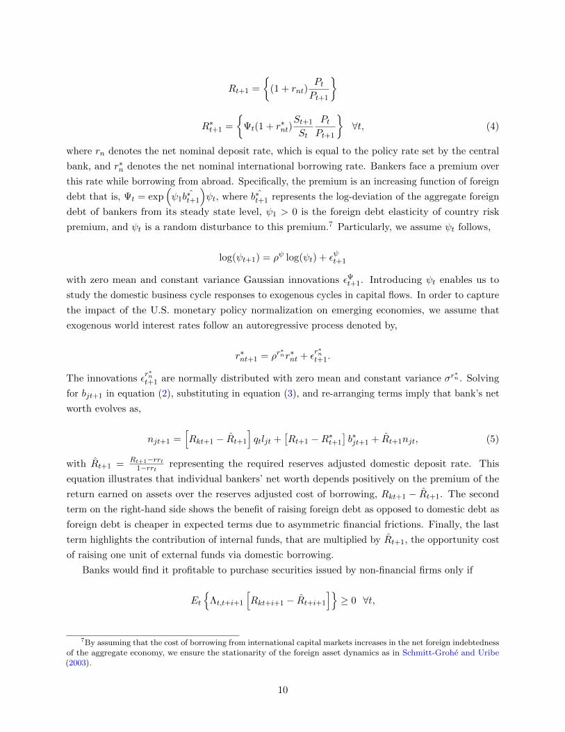
}∀t, (4)

where rn denotes the net nominal deposit rate, which is equal to the policy rate set by the central

bank, and r∗n denotes the net nominal international borrowing rate. Bankers face a premium over

this rate while borrowing from abroad. Specifically, the premium is an increasing function of foreign

debt that is, Ψt = exp(ψ1

ˆb∗t+1

)ψt, where ˆb∗t+1 represents the log-deviation of the aggregate foreign

debt of bankers from its steady state level, ψ1 > 0 is the foreign debt elasticity of country risk

premium, and ψt is a random disturbance to this premium.7 Particularly, we assume ψt follows,

log(ψt+1) = ρψ log(ψt) + εψt+1

with zero mean and constant variance Gaussian innovations εΨt+1. Introducing ψt enables us to

study the domestic business cycle responses to exogenous cycles in capital flows. In order to capture

the impact of the U.S. monetary policy normalization on emerging economies, we assume that

exogenous world interest rates follow an autoregressive process denoted by,

r∗nt+1 = ρr∗nr∗nt + ε

r∗nt+1.

The innovations εr∗nt+1 are normally distributed with zero mean and constant variance σr

∗n . Solving

for bjt+1 in equation (2), substituting in equation (3), and re-arranging terms imply that bank’s net

worth evolves as,

njt+1 =[Rkt+1 − Rt+1

]qtljt +

[Rt+1 −R∗t+1

]b∗jt+1 + Rt+1njt, (5)

with Rt+1 = Rt+1−rrt1−rrt representing the required reserves adjusted domestic deposit rate. This

equation illustrates that individual bankers’ net worth depends positively on the premium of the

return earned on assets over the reserves adjusted cost of borrowing, Rkt+1 − Rt+1. The second

term on the right-hand side shows the benefit of raising foreign debt as opposed to domestic debt as

foreign debt is cheaper in expected terms due to asymmetric financial frictions. Finally, the last

term highlights the contribution of internal funds, that are multiplied by Rt+1, the opportunity cost

of raising one unit of external funds via domestic borrowing.

Banks would find it profitable to purchase securities issued by non-financial firms only if

Et

{Λt,t+i+1

[Rkt+i+1 − Rt+i+1

]}≥ 0 ∀t,

7By assuming that the cost of borrowing from international capital markets increases in the net foreign indebtednessof the aggregate economy, we ensure the stationarity of the foreign asset dynamics as in Schmitt-Grohe and Uribe(2003).

10

where Λt,t+i+1 = βi+1[Uc(t+i+1)Uc(t)

]denotes the i + 1 periods-ahead stochastic discount factor of

households, whose banker members operate as financial intermediaries. Notice that in the absence

of financial frictions, an abundance in intermediated funds would cause Rk to decline until this

premium is completely eliminated. In the following, we also establish that

Et{

Λt,t+i+1

[Rt+i+1 −R∗t+i+1

]}> 0 ∀t,

so that the cost of domestic debt entails a positive premium over the cost of foreign debt at all

times.

In order to rule out any possibility of complete self-financing of bankers, we assume that bankers

have a finite life and survive to the next period only with probability 0 < θ < 1. At the end of each

period, 1− θ measure of new bankers are born and are remitted εb

1−θ fraction of the assets owned by

exiting bankers in the form of start-up funds.

3.2.2 Net worth maximization

Bankers maximize expected discounted value of the terminal net worth of their financial firm

Vjt, by choosing the amount of security claims purchased ljt and the amount of foreign debt b∗jt+1.

For a given level of net worth, the optimal amount of domestic deposits can be solved for by using

the balance sheet. Bankers solve the following value maximization problem,

Vjt = maxljt+i,b∗jt+1+i

Et

∞∑i=0

(1− θ)θiΛt,t+1+i njt+1+i,

which can be written in recursive form as,

Vjt = maxljt,b∗jt+1

Et

{Λt,t+1[(1− θ)njt+1 + θVjt+1]

}. (6)

For a non-negative premium on credit, the solution to the value maximization problem of banks

would lead to an unbounded magnitude of assets. In order to rule out such a scenario, we follow

Gertler and Kiyotaki (2011) and introduce an agency problem between depositors and bankers.

Specifically, lenders believe that banks might renege on their liabilities and divert λ fraction of their

total divertable assets, where such assets constitute total loans minus a fraction ωl of domestic

deposits. When lenders become aware of the potential confiscation of assets, they would initiate

a bank run and lead to the liquidation of the bank altogether. In order to rule out bank runs in

equilibrium, in any state of nature, bankers’ optimal choice of ljt should be incentive compatible.

Therefore, the following constraint is imposed on bankers,

Vjt ≥ λ(qtljt − ωlbjt+1

), (7)

where λ and ωl are constants between zero and one. This inequality suggests that the liquidation

cost of bankers from diverting funds Vjt, should be greater than or equal to the diverted portion of

11

assets. In equilibrium, bankers never divert (and default on) funds and accordingly adjust their

demand for external finance to meet the incentive compatibility constraint in each period.

We introduce asymmetry in financial frictions by excluding ωl fraction of domestic deposits from

diverted assets. This is due to the idea that domestic depositors would arguably have a comparative

advantage over foreign depositors in recovering assets in case of a bankruptcy. Furthermore, they

would also be better equipped than international lenders in monitoring domestic bankers (see Section

4.3 for further details.)

Our methodological approach is to approximate the stochastic equilibrium around the determin-

istic steady state. Therefore, we are interested in cases in which the incentive constraint of banks is

always binding, which implies that (7) holds with equality. This is the case in which the loss of

bankers in the event of liquidation is just equal to the amount of assets that they can divert.

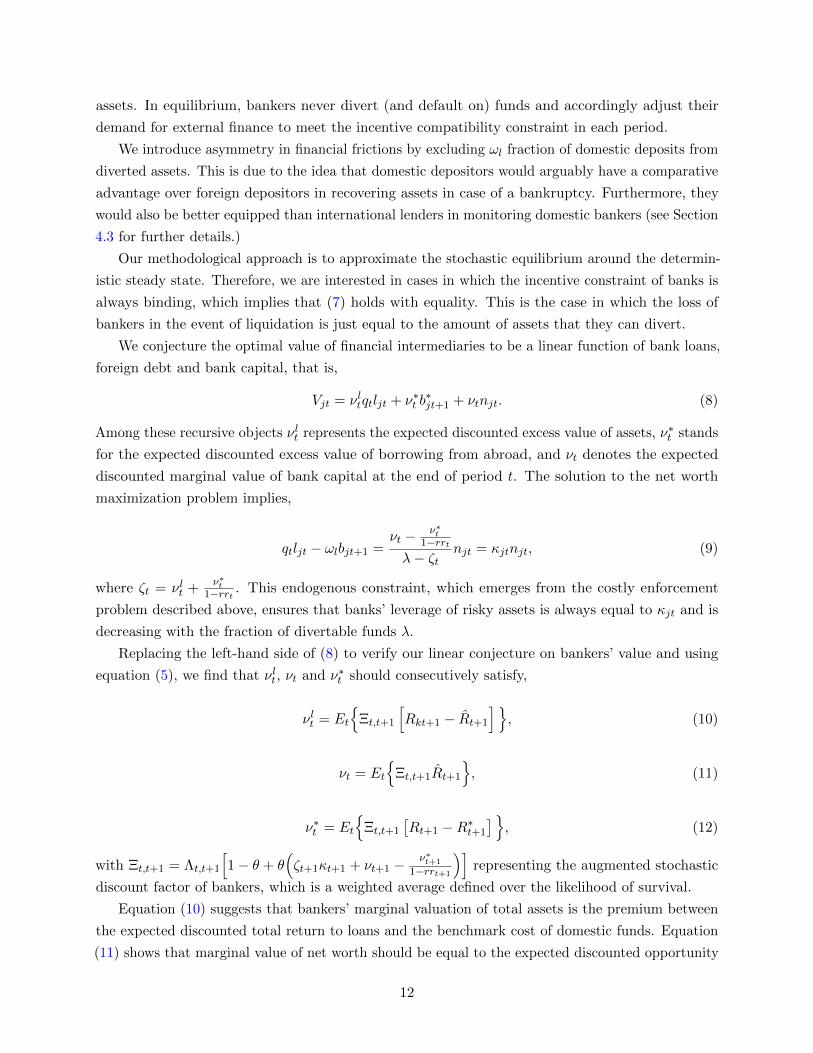
We conjecture the optimal value of financial intermediaries to be a linear function of bank loans,

foreign debt and bank capital, that is,

Vjt = νltqtljt + ν∗t b∗jt+1 + νtnjt. (8)

Among these recursive objects νlt represents the expected discounted excess value of assets, ν∗t stands

for the expected discounted excess value of borrowing from abroad, and νt denotes the expected

discounted marginal value of bank capital at the end of period t. The solution to the net worth

maximization problem implies,

qtljt − ωlbjt+1 =νt − ν∗t

1−rrtλ− ζt

njt = κjtnjt, (9)

where ζt = νlt +ν∗t

1−rrt . This endogenous constraint, which emerges from the costly enforcement

problem described above, ensures that banks’ leverage of risky assets is always equal to κjt and is

decreasing with the fraction of divertable funds λ.

Replacing the left-hand side of (8) to verify our linear conjecture on bankers’ value and using

equation (5), we find that νlt, νt and ν∗t should consecutively satisfy,

νlt = Et

{Ξt,t+1

[Rkt+1 − Rt+1

]}, (10)

νt = Et

{Ξt,t+1Rt+1

}, (11)

ν∗t = Et

{Ξt,t+1

[Rt+1 −R∗t+1

] }, (12)

with Ξt,t+1 = Λt,t+1

[1− θ + θ

(ζt+1κt+1 + νt+1 −

ν∗t+1

1−rrt+1

)]representing the augmented stochastic

discount factor of bankers, which is a weighted average defined over the likelihood of survival.

Equation (10) suggests that bankers’ marginal valuation of total assets is the premium between

the expected discounted total return to loans and the benchmark cost of domestic funds. Equation

(11) shows that marginal value of net worth should be equal to the expected discounted opportunity

12

cost of domestic funds, and lastly, equation (12) demonstrates that the excess value of raising foreign

debt is equal to the expected discounted value of the premium in the cost of raising domestic debt

over the cost of raising foreign debt. One can show that this spread is indeed positive, that is, ν∗t > 0

by studying first order condition (A.13) in Online Appendix A.2 and observing that λ, µ, ωl > 0,

and rrt < 1 with µ denoting the Lagrange multiplier of bankers’ problem.

The definition of the augmented pricing kernel of bankers is useful in understanding why banks

shall be a veil absent financial frictions. Specifically, the augmented discount factor of bankers can

be re-written as Ξt,t+1 = Λt,t+1

[1− θ+ θλκt+1

]by using the leverage constraint. Financial frictions

would vanish when none of the assets are diverted, i.e. λ = 0 and bankers never have to exit, i.e.

θ = 0. Consequently, Ξt,t+1 simply collapses to the pricing kernel of households Λt,t+1. This case

would also imply efficient intermediation of funds driving the arbitrage between the lending and

deposit rates down to zero. The uncovered interest parity on the other hand, is directly affected by

the asymmetry in financial frictions. That is, as implied by equation (12), the uncovered interest

parity obtains only when ν∗t = 0.

3.2.3 Aggregation

We confine our interest to equilibria in which all households behave symmetrically, so that we

can aggregate equation (9) over j and obtain the following aggregate relationship:

qtlt − ωlbt+1 = κtnt, (13)

where qtlt, bt+1, and nt represent aggregate levels of bank assets, domestic deposits, and net worth,

respectively. Equation (13) shows that the aggregate credit net of non-divertable domestic deposits

can only be up to an endogenous multiple of the aggregate bank capital. Furthermore, fluctuations

in asset prices qt, would feed back into fluctuations in bank capital via this relationship. This would

be the source of the financial accelerator mechanism in our model.

The evolution of the aggregate net worth depends on that of the surviving bankers net+1, which

might be obtained by substituting the aggregate bank capital constraint (13) into the net worth

evolution equation (5), and adding up the start-up funds of the new entrants nnt+1. The latter is

equal to εb

1−θ fraction of exiting banks’ assets (1− θ)qtlt. Therefore, nnt+1 = εbqtlt. As result, the

transition for the aggregate bank capital becomes, nt+1 = net+1 + nnt+1.

3.3 Monetary authority and the government

The monetary authority sets the short-term nominal interest rate via a simple (and imple-

mentable) monetary policy rule that includes only a few observable macroeconomic variables and

ensures a unique rational expectations equilibrium.8 We consider Taylor-type interest rate rules

that respond to deviations of an augmenting variable ft in addition to inflation and output from

their steady state levels,

8For further discussion on simple and implementable rules, see Schmitt-Grohe and Uribe (2007).

13

log

(1 + rnt1 + rn

)= ρrn log

(1 + rnt−1

1 + rn

)+ (1− ρrn)

[ϕπ log

(1 + πt1 + π

)+ ϕy log

(yty

)+ ϕf log

(ft

f

)],

(14)

where rnt is the short-term policy rate, πt is the net CPI inflation rate, yt is home output, variables

with bars denote respective steady state values that are targeted by the central bank, and ft

corresponds to the level of bank credit, asset prices, real exchange rate, credit spreads or the U.S.

interest rate in alternative specifications. In each specification, ϕf measures the responsiveness of

the interest rate rule to the augmenting variable of interest. To be general, we allow for persistence

in the monetary policy rule so that 0 ≤ |ρrn | < 1.

In the benchmark specification, we assume that the required reserves ratio is fixed at rrt = rr ∀t,with rr denoting a steady state level. In Section 4.8 we investigate whether reserve requirements

can be used in combination with conventional monetary policy to reduce the procyclicality of the

financial system. In particular, we assume that required reserves ratios for both domestic and

foreign deposits respond to deviations of the loan-foreign deposits spread from its steady state value.

That is,

log

(1 + rrt1 + rr

)= ρrr log

(1 + rrt−1

1 + rr

)+ (1− ρrr)

[ϕrr log

(Rkt+1 −R∗t+1

Rk −R∗

)], (15)

with 0 < |ρrr| < 1 and ϕrr is a finite real number. Notice that credit spreads are countercyclical,

since the magnitude of intermediated funds decline in response to adverse shocks. Therefore, one

might conjecture that the reserve requirement rule would support the balance sheet of bankers in

bad times by reducing the effective tax on domestic and foreign liabilities as in Glocker and Towbin

(2012) and Mimir et al. (2013), implying a negative value for the optimized response coefficient ϕrr.

Money supply in this economy is demand determined and compensates for the cash demand of

workers and the required reserves demand of bankers. Consequently, the money market clearing

condition is given by

M0t = Mt + rrtBt+1,

where M0t denotes the supply of monetary base in period t. As discussed by Schmitt-Grohe and

Uribe (2007), the inclusion of cash balances would not alter the optimality of interest rate policy

rules.

Government consumes a time-varying fraction of home goods gHt that follows the exogenous

process

ln(gHt+1) = (1− ρgH ) ln gH + ρgH

ln(gHt ) + εgH

t+1,

where εgH

t+1 is a Gaussian process with zero mean and constant variance. We introduce this shock to

capture disturbances in domestic aggregate demand that create a trade-off for the monetary policy

in responding to inflation or output.

14

The fiscal and monetary policy arrangements lead to the consolidated government budget

constraint,

pHt gHt y

Ht =

Mt −Mt−1

Pt+rrtBt+1 − rrt−1Bt

Pt+TtPt.

Lump-sum taxes τt = TtPt

are determined endogenously to satisfy the consolidated government budget

constraint at any date t. The resource constraints and the definition of competitive equilibrium are

included in Online Appendix A.

4 Quantitative analysis

This section analyzes quantitative predictions of the model by studying the results of numerical

simulations of an economy calibrated to a typical emerging market, Turkey, for which financial

frictions in the banking sector and monetary policy tools analyzed here are particularly relevant. To

investigate the dynamics of the model and carry out welfare calculations, we compute a second-order

approximation to the equilibrium conditions. All computations are conducted using the open source

package, Dynare.

4.1 Model parameterization and calibration

Table 2 lists the parameter values used for the quantitative analysis of the model economy.

The reference period for the long-run ratios implied by the Turkish data is 2002-2014. The data

sources for empirical targets are the Central Bank of the Republic of Turkey (CBRT, hereafter) and

the Banking Regulation and Supervision Agency. The preference and production parameters are

standard in the business cycle literature. Starting with the former, we set the quarterly discount

factor β = 0.9821 to match the average annualized real deposit rate of 7.48% observed in Turkey

over the sample period. The relative risk aversion σ = 2 is taken from the literature. We calibrate

the relative utility weight of labor χ = 199.348 in order to fix hours worked in the steady state at

0.3333. The Frisch elasticity of labor supply parameter ξ = 3 and the habit persistence parameter

hc = 0.7 are set to values commonly used in the literature. The relative utility weight of money

υ = 0.0634 is chosen to match 2.25 as the quarterly output velocity of M2. Following the discussion

in Faia and Monacelli (2007), we set the intratemporal elasticity of substitution for the consumption

composite γ = 0.5. The intratemporal elasticity of substitution for the investment composite good

γi = 0.25 is chosen as in Gertler et al. (2007). The share of domestic goods in the consumption

composite ω = 0.62 is set to match the long-run consumption-to-output ratio of 0.57.

We calibrate the financial sector parameters to match some long-run means of financial variables

for the 2002-2014 period. Specifically, the fraction of assets that can be diverted λ = 0.65, the

proportional transfer to newly entering bankers εb = 0.00195, and the fraction of domestic deposits

that cannot be diverted ωl = 0.81 are jointly calibrated to match the following three targets: an

average domestic credit spread of 34 basis points, which is the difference between the quarterly

15

commercial loan rate and the domestic deposit rate, an average bank leverage of 7.94, and the share

of foreign funds in total bank liabilities, which is around 40% for commercial banks in Turkey. We

also pick the survival probability of bankers θ as 0.925, which implies an average survival duration

of nearly three and a half years for bankers.

Regarding the technology parameters, the share of capital in the production function α = 0.4

is set to match the share of labor income in Turkey. We pick the share of domestic goods in the

investment composite ωi = 0.87 to match the long-run mean of investment-to-output ratio of 15%.

The steady state utilization rate is normalized at one and the quarterly depreciation rate of capital

δ = 3.5% is chosen to match the average annual investment-to-capital ratio. The elasticity of

marginal depreciation with respect to the utilization rate % = 1 is set as in Gertler et al. (2007). The

investment adjustment cost parameter is calibrated to ψ = 5, which implies a long-run elasticity of

the price of capital with respect to the investment-to-capital ratio of 0.125, which is in line with the

literature. We set the elasticity of substitution between varieties in final output ε = 11 to have a

steady state mark-up value of 1.1. Rotemberg price adjustment cost parameters in domestic and

foreign intermediate goods production ϕH = ϕF = 113.88 are chosen to imply a probability of 0.75

of not changing prices in both sectors. We pick the elasticity of export demand with respect to

foreign prices Γ = 1 and the foreign output share parameter νF = 0.25 as in Gertler et al. (2007).

Given these parameters, the mean of foreign output y∗ = 0.16 is chosen to match the long-run mean

of exports-to-output ratio of 18%.

We estimate a standard Taylor rule for the Turkish economy to approximate the monetary policy

implemented in Turkey. In the estimation, we use the CBRT’s average funding rate, which is the

effective policy rate, over the period 2003-2014. The resulting estimated interest rate rule persistence

is ρrn = 0.89 and the inflation rate response is ϕπ = 2.17. The estimated response coefficient

of output turned out not to be statistically different from zero. We then use these estimated

parameters to calibrate the standard Taylor rule parameters in the model of the decentralized

economy. Moreover, the long-run value of required reserves ratio rr = 0.09 is set to its time series

average level for the period 1996-2015. The steady state government expenditures-to-output ratio

gH = 10% reflects the value implied by the Turkish data for the 2002-2014 period.

Finally, we estimate three independent AR(1) processes for the share of public demand for home

goods gHt , country risk premium Ψt+1 and the U.S. interest rate R∗nt+1, where εgH

t+1, εΨt+1, and εR∗nt+1

are i.i.d. Gaussian shocks. We use J.P. Morgan’s EMBI Global Turkey data in the estimation of

country risk premium shocks. The resulting estimated persistence parameters are ρgH

= 0.457,

ρΨ = 0.963, and ρR∗n = 0.977. The estimated standard deviations are σg

H= 0.04, σΨ = 0.0032,

and σR∗n = 0.001. The long-run mean of quarterly foreign interest rate is set to 64 basis points to

match quarterly interest rate in the U.S. for the period 1996-2014 and the long-run foreign inflation

rate is set to zero. The foreign debt elasticity of risk premium is set to ψ1 = 0.015. Parameters

underlying the TFP shock are taken from Bahadir and Gumus (2014), who estimate an AR(1)

process for the Solow residuals coming from tradable output in Turkey for the 1999:Q1-2010:Q1

period. Their estimates for the persistence and volatility of the tradable TFP emerge as ρA = 0.662

16

and σA = 0.0283. Finally, we calibrate the export demand shock process under all shocks to match

both the persistence and the volatility of GDP of the European Union, which are 0.31 and 0.48%

respectively.9 The implied persistence and volatility parameters are ρy∗

= 0.977 and σy∗

= 0.0048.

4.2 Model versus data

The quantitative performance of the decentralized model economy operating under the standard

Taylor calibrated to the Turkish data is illustrated in Table 3, in which the relative volatilities,

correlations with output and autocorrelations of the simulated time series are compared with

corresponding moments implied by the data. The first column of the table shows that for the

reference time period, consumption is less volatile than output, whereas investment is more volatile

in the data. When financial variables are considered, we observe that credit spreads are less volatile

than output, whereas bankers’ foreign debt share and loans are more volatile. The data also suggest

that the real exchange rate is more volatile than output, while the current account- and trade

balance-to-output ratios are less volatile. Finally, inflation and policy rates are less volatile than

output in the data. The second column of Table 3 reports that despite the benchmark model is

not estimated and includes a few number of structural shocks, it is able to generate the relative

volatilities of model variables of interest that are mostly inline with the data.

When the correlations with output and autocorrelations are considered, the benchmark model

performs well on quantitative grounds as well. Columns 3 and 4 imply that the model is able

to generate same signs for correlations of all model variables in interest with output. Most

importantly, credit spreads, real exchange rate, current account balance-to-GDP ratio and inflation

are countercyclical, whereas bank credit, investment and consumption are procyclical. Furthermore,

apart from the short-term interest rate, the level of model implied correlation coefficients are fairly

similar to those implied by the data. These patterns are also observed for the model generated

autocorrelations in comparison to the data, as shown in the last two columns of the table.

Table 4 reports asymptotic variance decomposition of main model variables under domestic

and external shocks operating simultaneously. The unconditional variance decomposition results

illustrate that country risk premium and world interest rate shocks explain most of the variation

in financial and external variables as well as a considerable part of the variation in the inflation

and the short-term interest rates. Remarkably, the U.S. interest rate shocks in isolation explain

about 12% of the variation in model variables on average, whereas the explanatory power of country

premium shocks are much stronger, which is fairly different than what the findings of Uribe and

Yue (2006) suggest. TFP shocks, on the other hand, roughly account for one-third of volatilities in

output, credit and the inflation rate, and a quarter of the variation in policy rates. Export demand

and government spending shocks drive a negligible part of fluctuations in model variables with the

only exception of the spending shocks’ declining effect on output as the horizon gets longer. These

9We use the GDP of the European Union (EU) for the calibration of export demand shocks because it is the maintrading partner of Turkey with the largest share in the data over the past decade. The average share of the EU inTurkey’s exports is 46% over the period from 2007 to 2016. The trade data are taken from the Turkish StatisticalAgency (www.tuik.gov.tr).

17

patterns are also confirmed for one-quarter and one-year ahead conditional variance decompositions

(reported in Table B.1 in Online Appendix B). Notice that the variance decomposition analysis is

sensitive to the calibrated size of individual shocks. However, it is informative in order to sharpen

our focus on the importance of external shocks.

We further assess the quantitative performance of the calibrated model by analyzing impulse

responses of model simulations to an exogenous increase in the country risk premium of 127 basis

points, which is at the ballpark of what EMEs have experienced during the taper tantrum in May

2013. The straight plots in Figure 2 are the impulse responses of model variables in the benchmark

economy with the calibrated inflation targeting rule. The initial impact of the country borrowing

premium shock is reflected on the real exchange rate in the direction of a sharp depreciation of

5%, which amplifies the increase in the cost of foreign borrowing. The resulting correction in the

cyclical component of current account balance-to-output ratio is about 0.75%. In line with capital

outflows, bankers’ share of foreign debt declines more than 3% in 18 quarters. The pass-through

from increased nominal exchange rate depreciation leads to a rise in inflation by about 1 percentage

point per annum. Banks cannot substitute foreign funds with domestic deposits easily as domestic

debt is more expensive than foreign debt on average. Therefore, bankers’ demand for capital claims

issued by non-financial firms collapses, which ignites a 1.5% decline in asset prices.

The fall in asset prices feeds back into the endogenous leverage constraint, (13) and hampers

bank capital severely, 11% fall on impact. The tightening financial conditions and declining asset

prices in total, reduces bank credit by 1.5% on impact, and amplifies the decline in investment up to

more than 3% and output up to 0.7% in five quarters. Observed surges in credit spreads over both

domestic and foreign borrowing costs (by about 120 and 12 basis points per annum for loan-foreign

deposits and -domestic deposits spreads, respectively) reflect the tightened financial conditions in

the model. The decline in output and increase in inflation eventually calls for about 55 annualized

basis points increase in the short-term policy rate in the baseline economy. In conclusion, the model

performs considerably well in replicating the adverse feedback loop (illustrated in Figure 1) that

EMEs fell into in the aftermath of the recent global financial crisis.

For brevity, we do not explain in detail here the impulse responses of model variables under

the productivity, government spending, the U.S. interest rate and export demand shocks. Readers

may refer to Online Appendix B to see the impulse response functions of model variables under

each shock. However, we would like to note that most of the endogenous variables and the policy

instruments respond to each shock in a fairly standard way, in line with the previous literature.

4.3 Asymmetric financial frictions and the UIP

Under certain conditions, the UIP may not hold so that the exchange rate dynamics do not align

with interest rate differentials.10 In our framework, the agency problem between bankers and foreign

lenders are asymmetrically more intense compared to that between bankers and domestic depositors,

10See the Handbook chapter by Engel (2015) which lists a vast survey of contributions that consider departuresfrom the UIP.

18

which creates a wedge between the real costs of domestic and foreign debt.11 The analysis in Online

Appendix A.2 delivers this result analytically by observing that in equilibrium, the excess value of

borrowing from abroad ν∗ should be positive so that domestic depositors charge more compared to

international lenders. In this regard, asymmetric financial frictions in a small open economy provide

a microfoundation to stronger exchange rates than can be explained by the expected real interest

rate differentials under the UIP as elaborated by Engel (2016).

Figure 3 provides a graphical illustration of the workings of the asymmetry in financial frictions.

We plot the external funds market on the left panel of the figure in which there is an almost perfectly

elastic supply curve, and a downward sloped demand curve for foreign funds, absent financial

frictions. Indeed, the slope of the supply curve is slightly positive since the country risk premium

increases with the foreign debt. When λ > 0, the incentive compatibility constraint binds and

imposes a leverage constraint on banks. Therefore, the supply curve of foreign debt makes a kink

and becomes vertical at the equilibrium level of foreign debt b∗ω.

The panel on the right displays the domestic funds market and covers three cases regarding the

asymmetry in financial frictions. The supply curve in this market originates from the consumption-

savings margin of households and is upward sloped. When ωl = 0, financial frictions are symmetric

in both markets and the supply curve makes a kink at the equilibrium domestic debt level bω=0,

and becomes vertical. This case corresponds to the UIP condition so that there is no arbitrage

between the two sources of external finance, yielding Rk > R = R∗. When ωl takes an intermediate

value between zero and one, the demand schedule shifts to the right, as diverted assets constitute

a smaller portion of total assets, making banks able to borrow more. This results in a movement

along the workers’ deposits supply curve until R takes an intermediate value between the loan

rate and foreign borrowing rate Rk > R > R∗. Lastly, when ωl = 1, the domestic deposits market

becomes frictionless and the deposit supply curve becomes continuous rendering banks a veil from

the perspective of households. In this case, Rk = R > R∗, implying that depositing at a financial

intermediary is no different than directly investing in physical capital for households. This shifts

the equilibrium level of domestic debt further to the right to bω=1.

For simplicity, we did not plot the impact of changes in ωl on the amount of foreign debt. Indeed,

one shall expect that the share of foreign debt increases with ωl despite the increase in domestic

deposits. This is because ωl levers up bankers so that it facilitates smaller amounts of domestic

borrowing to bring enough relaxation of the financial constraint (7) in matching the excess cost of

domestic debt.12 Finally, in Figure 2 we explore the impact of the asymmetry in financial frictions

by using different ωl values. The value of ωl increases as we move along the dashed, straight, and

dotted-straight plots in which the straight plots correspond to the benchmark economy. As expected,

11Broner et al. (2014) show that when domestic borrowers discriminate against foreign creditors, a positive spreadbetween domestic and foreign interest rates emerges. Fornaro (2015) obtains a similar result in a setup with collateralconstraints by assuming that domestic borrowing does not require collateral.

12Steady state comparisons for different levels of asymmetry confirm this conjecture that liability composition ofbankers becomes more biased towards foreign debt as ωl increases.

19

we find that the volatility of macroeconomic and financial variables, as well as monetary variables

gets smaller as the fraction of non-divertable domestic deposits increases.

4.4 Model frictions and optimal monetary policy

The model economy includes six key ingredients that generate deviations from a first-best flexible

price economy apart from the real rigidities such as habit persistence, variable capacity utilization

and investment adjustment costs. Among these, monopolistic competition and price rigidities

are standard in canonical closed-economy New-Keynesian models, whereas open-economy New-

Keynesian models additionally consider home bias and incomplete exchange rate pass-through.13

These frictions distort the intratemporal consumption-leisure margin. Our model also includes credit

frictions in the banking sector and a risk premium in the country borrowing rate. These additional

frictions distort the intertemporal consumption-savings margin.

Intratemporal wedge: In the closed, first-best flexible price economy, the intratemporal efficiency

requires that

MRStMPLt

=−Uh(t)/Uc(t)

Wt/Pt= 1 (16)

The model counterpart of the consumption-leisure margin is found by combining and manipulating

equations (A.2), (A.8), (A.22), (A.23) and (A.28) listed in Online Appendix A, which yields

MRStMPLt

=−Uh(t)/Uc(t)

Wt/Pt=

(pHt + ηt)

X, (17)

with the expressions,

pHt =

[ω

1− (1− ω)(pFt )(1−γ)

]− 1(1−γ)

, (18)

pFt = Xst +ϕF

ε− 1

πFt (πFt − 1)

yFt− ϕF

ε− 1Et

{Λt,t+1

πFt+1(πFt+1 − 1)

yFt

}, (19)

X =ε

ε− 1, (20)

ηt =ϕH

ε− 1

πHt (πHt − 1)

yHt− ϕH

ε− 1Et

{Λt,t+1

πHt+1(πHt+1 − 1)

yHt

}. (21)

The first expression (18), is the relative price of home goods with respect to the aggregate price level

and it depends on ω, the home bias parameter. Under flexible home goods prices ϕH = 0, complete

exchange rate pass-through ϕF = 0, and no monopolistic competition X = 1, the intratemporal

13Galı (2008), Monacelli (2005), and Faia and Monacelli (2008) elaborate on these distortions in New Keynesianmodels in greater detail.

20

wedge becomes MRStMPLt

= −Uh(t)/Uc(t)Wt/Pt

= pHt . The case of pHt < 1 leads to an inefficiently low level

of employment and output as MRStMPLt

< 1. The case of ω = 1 corresponds to the closed economy in

which consumption basket only consists home goods and pHt = 1, restoring intratemporal efficiency.

Therefore, the Ramsey planner has an incentive to stabilize the fluctuations in pHt to smooth this

wedge, which creates a misallocation between consumption demand and labor supply.

The second expression (19), is the relative price of foreign goods with respect to the aggregate

price level, which depends on the gross markup X, the real exchange rate st, and an expression

representing incomplete exchange rate pass-through that originates from sticky import prices ϕF > 0.

If import prices are fully flexible ϕF = 0, and there is perfect competition X = 1, then pFt = st so

that there is complete exchange rate pass-through. However, even if that is the case, the existence

of the real exchange rate in the intratemporal efficiency condition still generates a distortion,

depending on the level of home bias ω. The Ramsey planner would then want to contain fluctuations

in the real exchange rate (which are equivalent to endogenous cost-push shocks as discussed by

Monacelli (2005)) to stabilize this wedge. Furthermore, if import prices are sticky ϕF > 0, the

law-of-one-price-gap might potentially reduce pHt below 1, creating an additional distortion in the

intratemporal wedge. Therefore, optimal policy requires stabilization of the deviations from the law

of one price, inducing smoother fluctuations in exchange rates.

The final expression (21), stems from the price stickiness of home goods. Unless ηt is always

equal to X, the intratemporal efficiency condition will not hold, leading to a welfare loss. ηt = X

for all t is not possible since price dispersion across goods, which depends on inflation, induces

consumers to demand different levels of intermediate goods across time. Moreover, menu costs that

originate from sticky home goods and import prices generate direct output losses. Consequently,

the planner has an incentive to reduce inflation volatility, which helps contain the movements in the

price dispersion.

Overall, in an open economy, price stability requires an optimal balance between stabilizing

domestic markup volatility induced by monopolistic competition and sticky prices and containing

exchange rate volatility induced by home bias and incomplete exchange rate pass-through.

Intertemporal wedge: In the closed, first-best flexible price economy with no financial frictions, the

intertemporal efficiency requires that

βEtRkt+1

[Uc(t+ 1)

Uc(t)

]= 1. (22)

Volatile credit spreads, the endogenous leverage constraint, fluctuations in the exchange rate,

and the existence of country risk premium result in deviations of the model counterpart of the

consumption-savings margin from what the efficient allocation suggests. Specifically, combining

conditions (4), (A.12), (A.13), and (10) under no reserve requirements rrt = 0, implies

βEtRkt+1

[Uc(t+ 1)

Uc(t)

]= (1 + τ1

t+1 − τ2t+1) > 1, (23)

21

with the expressions

τ1t+1 =

[cov[Ξt,t+1, (Rkt+1 −Rt+1)] + cov[Ξt,t+1, (Rt+1 −R∗t+1)]− λ µt

(1+µt)

]Et[Ξt,t+1]

> 0, (24)

τ2t+1 = Et[R

∗nt+1]Et

[Ψt+1

St+2

St+1

Pt+1

Pt+2

]+ cov

{R∗nt+1,

[Ψt+1

St+2

St+1

Pt+1

Pt+2

]}< 0, (25)

where µt is the Lagrange multiplier of the incentive compatibility constraint faced by bankers and

the signs of τ1t+1 and τ2

t+1 are confirmed by simulations.

The first expression τ1t+1, which contributes to the intertemporal wedge, originates from the

financial frictions in the banking sector. In particular, the first term in τ1t+1 is the risk premium

associated with the credit spread over the domestic cost of borrowing, the second term is the risk

premium associated with the funding spread, and the last term is the liquidity premium associated

with binding leverage constraints of banks. When credit frictions are completely eliminated λ = 0,

both covariances and the last term in the numerator of τ1t+1 become zero.14 The Ramsey planner

has an incentive to contain the fluctuations in credit spreads over both domestic and foreign deposits

to smooth this wedge by reducing movements in the Lagrange multiplier of the endogenous leverage

constraint.

The second expression τ2t+1 is the remaining part of the intertemporal wedge, stemming from

openness and the country borrowing premium. The second term in this wedge is the risk premium

associated with the U.S. interest rate and the real exchange rate movements. It is strictly negative

because increases in the foreign interest rate R∗nt+1 reduces foreign borrowing and diminishes the

debt elastic country risk premium Ψt+1. Furthermore, the magnitude of the real exchange rate

depreciation gradually declines after the initial impact of shocks. Consequently, the optimal policy

requires containing inefficient fluctuations in the exchange rate, which would reduce fluctuations in

foreign debt and the country borrowing premium, accordingly. This channel is typically referred to

as the financial channel by which exchange rate depreciation hurts the balance sheets of borrowers

who suffer from liability dollarization, leading them to curb domestic demand as discussed by Kearns

and Patel (2016).

Overall, in an open economy with financial frictions, financial stability requires an optimal

balance between stabilizing credit spreads volatility induced by financial frictions, which distorts

the dynamic allocation between savings and investment, and containing exchange rate volatility

induced by openness, incomplete exchange rate pass-through and financial frictions, which leads to

balance sheet deterioration. Therefore, the policymaker may want to deviate from fully stabilizing

credit spreads by reducing the policy rate and resort to some degree of exchange rate stabilization

by increasing the policy rate in response to adverse external shocks.

14When the UIP holds ωl = 0, the second covariance disappears. Nevertheless, the overall wedge would increasesubstantially, since more of the total external finance can be diverted. On the other hand, when none of domesticdeposits are diverted ωl = 1, the first covariance term disappears, leading the wedge to be smaller.

22

Finally, there exists an inherent trade-off between price stability and financial stability. The

policymaker may want to hike the policy rate in response to adverse external shocks to contain the

rise in the inflation rate coming from the exchange rate depreciation and the fall in the production

capacity of the economy at the expense of not being able to smooth fluctuations in lending spreads

and to reduce the cost of funds for banks. Below we validate this discussion by solving the Ramsey

planner’s problem and quantitatively shed light on how she optimally balances the tensions across

these trade-offs.

4.5 Long-run and cyclical properties of the decentralized and Ramsey economies

We assume that the Ramsey planner chooses state-contingent allocations, prices and policies to

maximize lifetime utility of households, taking the private sector equilibrium conditions (except the

monetary policy rule) and exogenous stochastic processes{At, g

Ht , ψt, r

∗nt, y

∗t

}∞t=0

as given. She uses

the short-term nominal interest rates as her policy tool to strike an optimal balance across different

distortions analyzed in the previous section and can only achieve second-best allocations. We solve

the optimal policy problem from a timeless perspective following Woodford (2003). We compute a

second-order approximation to the solution of the Ramsey planner’s problem.

We compare the non-stochastic steady states of decentralized and Ramsey economies in Table 5

to understand the sources of long-run welfare costs. Most strikingly, the Ramsey planner reduces

the exchange rate risk that bankers are exposed to by significantly lowering the ratio of foreign debt

to total liabilities. This relaxes financial constraints of banks since domestic debt is diverted less.

Consequently, the long run levels of bank leverage, credit, investment, consumption and output are

higher in the Ramsey economy. In this regard, our work places in the strand of literature surveyed

by Engel (2014) that calls for a direct targeting of currency for financial stability goals as well as its

indirect impact on inflation gap. Finally, the Ramsey steady state features a negative inflation rate

of -0.52% per annum compared to the decentralized economy, which is calibrated to an inflation rate

of zero.15 This results in a lower steady state markup and larger real money balances in the Ramsey

economy with respect to the decentralized economy. Resembling the findings of Schmitt-Grohe and

Uribe (2007), although the second-best economy exhibits deflation, we observe that the Ramsey

steady state emerges closer to eliminating price rigidity, rather than driving nominal interest rates

down to zero, since the Friedman rule suggests a deflation rate of 6.97% per annum.

We then analyze the dynamics of the decentralized and Ramsey economies in order to gauge the

source of short-run welfare costs. The intratemporal and intertemporal wedges in the model fluctuate

due to movements in the credit spreads over domestic and foreign deposits, the real exchange rate,

and the aggregate markup. Table 6 displays the relative volatilities of real, financial, external and

monetary variables in the decentralized and the planner’s economies. The results suggest that the

planner is able to smooth the fluctuations in variables that are related to the distortionary wedges.

In particular, she reduces the relative volatilities of the CPI inflation, aggregate markup, and the

15Schmitt-Grohe and Uribe (2007) finds a Ramsey steady-state inflation of -0.55% per annum, which is fairly closeto our case.

23

real exchange rate by 68%, 36%, and 63% compared to the decentralized economy, respectively.

Moreover, the planner is able to reduce the relative volatilities of lending spreads over domestic and

foreign deposits by 10% and 62% relative to the decentralized economy, respectively. Taking these

into account together with lower volatility in the real exchange rate, the results indicate that the

planner is able to contain fluctuations in both wedges. Finally, we observe a substantial decline in

the relative volatilities of bank leverage and bank net worth, mainly due to the lower volatilities of

lending spreads and the real exchange rate.

4.6 Welfare analysis

We assess the performances of alternative policy regimes by calculating the welfare cost associated

with a particular monetary policy rule relative to the time-invariant stochastic equilibrium of the

Ramsey policy. Before going into the details of the welfare computation, we want to emphasize

that our model economy features distortions due to monopolistic competition and financial frictions

in the banking sector even at its non-stochastic steady state. Following Schmitt-Grohe and Uribe

(2007), we do not assume any subsidy to factor inputs that removes the inefficiency introduced by

monopolistic competition. In addition, the distortions due to credit frictions are also present at

the deterministic steady state of the model. Therefore, we conduct our welfare analysis around

a distorted steady state and the constrained Ramsey planner can only achieve the second-best

allocation.

Conducting welfare evaluations around an inefficient steady state requires us to implement a

second-order approximation to the policy functions and the aggregate welfare in order to correctly

rank alternative policy regimes and to obtain accurate welfare costs. Otherwise, aggregate welfare

values would be the same across different policy rules since the mean values of endogenous variables

are equal to their non-stochastic steady state levels under a first-order approximation to the policy

functions.

We first define the welfare associated with the time-invariant equilibrium associated with the

Ramsey policy conditional on a particular state of the economy in period 0 as

V R0 = E0

∞∑t=0

βtU(cRt , hRt ,m

Rt ), (26)

where E0 denotes conditional expectation over the initial state, and cRt , hRt , and mRt stand for

the contingent plans for consumption, labor, and real money balances under the Ramsey policy.

Moreover, the welfare associated with the time-invariant equilibrium associated with a particular

policy regime conditional on a particular state of the economy in period 0 as

V A0 = E0

∞∑t=0

βtU(cAt , hAt ,m

At ), (27)

where cAt , hAt , and mAt stand for the contingent plans for consumption, labor and real money balances

under a particular alternative policy rule.

24

We then compute the welfare cost for each alternative monetary policy rule in terms of changes

that compensate consumption variation relative to the Ramsey policy. Let λc stand for the welfare

cost of implementing a particular monetary policy rule instead of the Ramsey policy conditional on

a particular state in period 0. We define λc as the proportional reduction in the Ramsey planner’s

consumption plan that a household must forgo to be as well off under policy regime A. Therefore,

λc is implicitly defined by

V A0 = E0

∞∑t=0

βtU((1− λc)cRt , hRt ,mR

t

). (28)

Hence, a positive value for λc implies that the Ramsey policy achieves a higher welfare relative to

the particular policy regime.

Finally, we define aggregate welfare in the following recursive form to conduct a second-order

approximation to V0:

V0,t = U(ct, ht,mt) + βEtV0,t+1. (29)

Schmitt-Grohe and Uribe (2007) show that V0 can also be represented as

V0,t = V0 +1

2∆(V0), (30)

where V0 is the level of welfare evaluated at the non-stochastic steady state and ∆(V0) is the constant

correction term, denoting the second-order derivative of the policy function for V0,t with respect to

the variance of shock processes. Therefore, equation (30) is an approximation to the welfare V0,t,

capturing the fluctuations of endogenous variables at the stochastic steady state.

4.7 Optimal simple and implementable policy rules

We search for optimal simple and implementable rules by following the methodology adopted

by Schmitt-Grohe and Uribe (2007). Specifically, we run a discrete grid search for alternative

optimal policy coefficients over the intervals ρrn ∈ [0, 0.995], ϕπ ∈ [1.001, 3], ϕy ∈ [0, 3], ϕf ∈ [−3, 3]

for f ∈ {credit, q, spr, s, R∗n}, ρrr ∈ [0, 0.995], and ϕrr ∈ [−3, 3]. Each interval includes 15 evenly

distributed grid points except for the intervals for the response coefficients of external and financial

variables as well as the interval for the response coefficient of the reserve requirement rule to credit

spreads. Those intervals include 30 evenly distributed grid points since we span both positive and

negative territories for their response coefficients. The boundary points of intervals are chosen by

following the literature and respecting technical constraints. In particular, we confine the smoothing

parameter of the interest rate rule to be positive and less than one to center our analysis on the

optimal responses to inflation, output and financial or external variables. We also choose the inertia

parameter of the reserve requirement rule to be positive and less than one. The lower bound for

inflation response is chosen to ensure determinacy. Following Schmitt-Grohe and Uribe (2007), the

upper bounds of the remaining response coefficients are chosen arbitrarily, but in the interest of

25

policymakers’ convenience in communicating policy responses, they are fixed at arguably not very

large magnitudes. We search for optimal set of policy coefficients for each shock separately and

under simultaneous shocks. The former experiment is informative for policymakers since it shows

how the optimal set of policy coefficients changes with the underlying set of disturbances. However,

the latter experiment might be more appealing in terms of actual policymaking because, in the real

world, the monetary authority cannot perfectly disentangle the different sources of business cycle

fluctuations. Section 4.8 covers optimal reserve requirement policies in addition to the interest rate

policy. In the interest of space, we left the discussion of optimal policy responses to domestic shocks

in isolation to the Online Appendix C.

4.7.1 External shocks

Table 7 displays the response coefficients of optimized conventional and augmented Taylor

rules, the absolute volatilities of key macroeconomic variables under these rules, and the associated

consumption-equivalent welfare costs relative to the Ramsey-optimal policy under country borrowing

premium, the U.S. interest rate and export demand shocks.

Optimized Taylor rules with and without smoothing feature no response to output variations

under external shocks with the exception of the rule without smoothing under export demand shocks.

This confirms the results discussed by Schmitt-Grohe and Uribe (2007) that positive response to

output is detrimental to welfare. The levels of the inflation coefficients on the other hand, are at

their lowest levels. This finding resembles the discussion of Aoki et al. (2016) that in response to

adverse external shocks (which already raise the cost of foreign debt) strong anti-inflationary stance

of interest rate policy would hurt bank balance sheets even more by increasing the cost of domestic

deposits. Since these policy rules do not target any financial stabilization objective, the volatilities

of inflation, credit spreads and the real exchange rate under these two optimized rules are much

higher than those under the Ramsey policy, which justifies relatively higher welfare costs associated

with these rules.

Table 7 indicates that under country risk premium shocks (which is the most relevant shock

as discussed in Section 4.2 for EMEs), the RER augmented rule which displays an aggressive and

positive response to fluctuations in the real exchange rate and only mild responses to inflation

and output variations implies the largest welfare among all optimized augmented Taylor rules (the

top panel). This optimal simple policy implies a welfare loss of 0.0015% vis-a-vis the Ramsey

policy. This suggests that considering the financial channel for an EME central bank is crucial

when domestic borrowers face currency mismatch. For this reason, the real exchange rate volatility

is smaller under this rule, than those implied by the other optimized Taylor rules. Since central

bank is already fighting the pass-through aggressively, it does not deem useful to take a strong

anti-inflationary stance. This is evident from the small degree of inflation volatility achieved under

this rule. This finding is also linked to the insights discussed by Monacelli (2005) and Monacelli

(2013) that under incomplete exchange rate pass-through, fluctuations in the exchange rate operate

26

as endogenous cost-push shocks (see equation (19)) and optimal policy deviates from maintaining

price stability towards exchange rate stability.

Lining up next is the optimized simple rule that augments asset prices. Our results confirm the

findings of Faia and Monacelli (2007) that optimal policy calls for a negative response to asset prices

together with a moderate anti-inflationary stance (with respective coefficients of -1.07 and 1.43). The

welfare cost implied by this policy rule is 0.0021% against the Ramsey policy. While the absolute

magnitude of the asset prices coefficient of optimal interest policy depends on the amplification

created by financial frictions, the intuition behind its negative sign primarily hinges on the existence

of investment adjustment costs. As discussed in the Online Appendix A.3, capital producers buy

the depreciated capital from intermediate goods firms and incur an investment adjustment cost that

is scaled up by the asset price q. This causes Tobin’s-q to operate as a procyclical tax on investment

and limits the expansion in investment to be smaller than the efficient magnitude in response to

favorable shocks. Therefore, an easing in the policy rate boosts investment demand of intermediate

goods producers and gets the dynamics of investment closer to the Ramsey allocation.16 Stronger

investment demand stimulated by the asset price-augmented interest rate policy rises equilibrium

asset prices more than the case with no policy response. Indeed, Table 7 and Figure 4 illustrate that

both the Ramsey policy and the asset price-augmented interest rate rule suggest a sharp increase in

the volatility of asset prices.17 Finally, the surge in demand by accommodative monetary policy

calls for an increase in the inflation rate under this rule compared to the optimized standard Taylor

rule (with respective coefficients of 1.43 and 1.001). Therefore, using an augmented policy rule with

financial stability considerations allows the central bank to take a stronger anti-inflationary stance.

We find that the loan-deposits spread-augmented Taylor rule achieves a level of welfare very close

to that of the asset price-augmented Taylor rule (the implied cost is 0.0026%). Interest rate policy

features a LATW role in this case because credit spreads are countercyclical and the optimized

augmented rule calls for an easing in bad times. Consequently, this rule justifies a higher inflation

response coefficient than the optimized standard Taylor rule. Under this rule, the volatility of credit

spreads is even lower than that in the Ramsey policy whereas the volatilities of the inflation rate

and the real exchange rate are much higher.

Our findings also show that optimized credit-augmented interest rate rules feature a negative

response to the level of credit. This result is mainly due to the fact that the decentralized economy

in the model features underborrowing rather than overborrowing compared to the Ramsey planner’s

economy as in Benigno et al. (2013). These authors show that introducing production might

transform the overborrowing observed in endowment economies to underborrowing, which in turn

16Our results seem to contrast with the findings of Gambacorta and Signoretti (2014) who find that an interestrate policy rule that is augmented with a positive response to asset prices performs better than a standard Taylorrule. However, they do not consider the negative range for the asset price response coefficient while searching forpolicy rules that minimize loss functions, which depend on inflation and output variability. Indeed, they obtain theminimum loss levels when this coefficient hits its lower bound of zero.

17This insight is akin to the Ramsey planner’s optimal policy of increasing volatility in labor income tax rateunder the existence of labor market distortions in order to bring fluctuations in employment closer to the efficientfluctuations. For a detailed elaboration, see Arseneau and Chugh (2012).

27

suggests that macroprudential taxes that are intended to reduce borrowing are detrimental to

welfare. Our steady state comparisons that are reported in Table 5 confirm this underborrowing

result. The table shows that the planner’s economy features a higher leverage compared to the

decentralized economy, which is achieved by collecting more deposits (higher borrowing of banking

sector). By having a higher leverage, the planner extends more credit to non-financial firms, leading

to more capital accumulation, higher investment and thus higher output in the economy. In this

environment, optimized credit-augmented monetary policy rule reduces the policy rate in response

to positive deviations of credit from its steady state level over the business cycle. This further

increases deposit issuance and credit extension, stimulates investment more and finally increases

output. Reducing policy rate in response to higher credit brings allocations in the decentralized

economy closer to those in the second best economy (i.e. the Ramsey planner’s economy). This

finding is consistent with that discussed by Benigno et al. (2013) since the macroprudential tax

on borrowing in their paper is akin to a policy rate hike in our model, which increases the cost of

borrowing for banks. While the optimized credit-augmented interest rules achieve a higher level of

welfare compared to the optimized standard Taylor rules, their implied welfare cost is larger than

those of the optimized RER- or credit spread-augmented interest rate rules.

Optimized augmented Taylor rules under the U.S. interest and export demand shocks display

very similar results as in the case of the country borrowing premium shocks. For brevity, we do not

discuss the results here in detail. We just would like to focus on the results of a particular augmented

Taylor rule. Specifically for the U.S. interest rate shocks, we also consider another optimized

augmented Taylor rule that directly responds to the U.S. policy rate movements in addition to

inflation and output variations. This rule is of particular interest for EME policymakers as domestic

policy rates in EMEs might be driven by the changes in the U.S. policy rate over and above domestic

factors would imply, which is also empirically shown by Takats and Vela (2014), and Hofmann and

Takats (2015). The latter paper suggests two reasons as to why EME policy rates might follow

those in the U.S. First, they might want to eliminate high interest differentials resulting from the

U.S policy rate movements, which may potentially cause exchange rate appreciation and hence a

deterioration in trade competitiveness. Second, they might want to prevent excessive short-term

capital inflows by eliminating large interest rate differentials in order to maintain financial stability.

The model results qualitatively confirm their empirical findings, suggesting that it is optimal for an

EME policymaker to positively respond to the U.S. policy rate. In response to an orthogonalized

100 basis points increase in the U.S. policy rate, we find that the EME central bank should raise its

policy rate by 257 basis points. However, the welfare cost implied by this policy rules is an order of

magnitude larger than those implied by the credit spread and the RER-augmented Taylor rules. On

the other hand, when compared to the optimized standard Taylor rules, the welfare cost implied by

this policy is much smaller (0.0096% vs. 0.3014%).

28

4.7.2 All shocks

Table 8 displays the response coefficients of optimized conventional and augmented Taylor

rules, the absolute volatilities of key macroeconomic variables under these rules, and the associated

consumption-equivalent welfare costs relative to the optimal Ramsey policy under domestic (TFP

and government spending) and external shocks hitting the economy simultaneously.

The optimized Taylor rules with and without smoothing still display zero response to output

deviations under all shocks. The magnitudes of the inflation response coefficients are at their lower

bounds and the optimized standard Taylor rule with smoothing still features a high degree of inertia.

Furthermore, these two optimized rules imply much more volatility in the CPI inflation rate and

the RER together with much less volatility in asset prices in comparison with the Ramsey policy,

which explains relatively higher welfare losses associated with these rules.

The findings associated with the optimized augmented Taylor rules suggest that a strong negative

response to asset prices together with an aggressive response to inflation achieves the highest welfare

possible. The associated welfare cost vis-a-vis the Ramsey policy is 0.0013%. It appears that the

gains are mainly linked to stimulating investment demand as this policy generates more asset price

volatility than that implied by the Ramsey policy. What follows the asset price augmenting rule

is the optimal rule that negatively responds to the credit spreads with an implied welfare cost

of 0.0027%. As in the case of external shocks, the gains associated with this rule depend on the

significant reduction in the volatility of credit spreads. Finally, we observe that the RER-augmented

Taylor rule implies a welfare cost in the same order of magnitude with the aforementioned policies

(0.0093%) and suggests a positive response to fluctuations in the real exchange rate with a mild

anti-inflationary stance. We also confirm our previous findings under other external shocks that it

is optimal to negatively respond to the level of credit and positively respond to the U.S. interest

rates, whereas these policy rules are dominated by the asset price-augmented interest rate policy.

Nevertheless, we find that in response to a 100 basis points increase in the U.S. policy rate, the EME

policy rate should be raised by 21 basis points (under simultaneous shocks), which is quantitatively

in line with the empirical findings of Hofmann and Takats (2015).

4.7.3 Optimal policy rules versus Ramsey-optimal policy

Figure 4 compares the impulses responses to a one standard deviation country risk premium

shock under the Ramsey planner’s economy (dashed plots) with the selected optimal simple interest

rate rules. In particular, we select the optimal real exchange rate-augmented interest rate rule

(straight plots) since it produces the smallest welfare cost vis-a-vis the Ramsey-optimal policy and

the optimal standard Taylor rule with smoothing (straight plots with asterisks) in order to highlight

the departures of conventional wisdom from optimality in our setup. We highlight the country risk

premium shock due to its strong explanatory power that emerged in the variance decomposition

analysis. For brevity, we do not plot the impulse responses to other domestic or external shocks,

which are available from the authors upon request.

29

The planner increases the policy rate by about 250 basis points per annum on impact in response

to a 127 basis points annualized increase in the country borrowing premium. Accordingly, both the

nominal and real exchange rates depreciate only about 2 percent, which contains the pass-through

to CPI inflation via imported goods. As a result, the annual CPI inflation rate falls a quarter of a

percentage point on impact in the planner’s economy, while it increases by 1 percentage point in the

decentralized economy (see straight plots in Figure 2). The Ramsey planner also contains inefficient

movements in the credit spreads over the cost of foreign debt and ensures that the credit spreads

increase by less than 100 basis points in annualized terms. This enables the planner to substantially

reduce the reversal in the current account balance. Notice that the second-best equilibrium warrants

increased volatility in asset prices and investment compared to the decentralized economy. In that

respect, the Ramsey planner trades-off a smoother path of the real exchange rate and credit spreads

against a more volatile trajectory for investment and output in order to achieve a more stable path

of the CPI inflation rate.

The optimal RER-augmented rule calls for an increase of 30 basis points in the policy rate in

annualized terms under the country borrowing premium shock. This results in 3 percent more

depreciation in the real exchange rate and 1 percentage point higher increase in the inflation rate

compared to the Ramsey-optimal policy. As a result, credit spreads rise more and there is a stronger

reversal in the current account balance in comparison to the second-best economy. However, this

optimized rule approximates the Ramsey-optimal policy fairly well in terms of bringing fluctuations

in the asset price, investment and output closer to efficient fluctuations. Recall that the real exchange

rate response coefficient of this optimized rule hits its upper bound of 3 (see the top panel of Figure

7) suggesting that this policy could approximate the Ramsey-optimal policy even better should we

allowed the response coefficient to take a larger value.

Since optimal Taylor rule with smoothing exhibits no response to the real exchange rate and

displays only a mild response to inflation, it calls for a negligible rise (by about only 2 basis

points per annum) in the short-term policy rate when the country risk premium shock hits the

economy. While the on-impact depreciation under this rule resembles that implied by the optimal

RER-augmented rule, currency exchanges at about a 1 percent more depreciated level under this

rule for 12 consecutive quarters. This results in 1.4 percentage point rise in the CPI inflation rate

on impact due to the pass-through and underpins the relatively larger welfare loss implied by this

rule. Since the tightening in the policy rate is much smaller under this rule, credit spreads rise even

less than the Ramsey-optimal policy. Consequently, the dynamics of investment and asset prices

implied by this rule deviate substantially from those produced by either the second-best economy or

the optimal exchange rate-augmented policy.

4.7.4 Optimal policy rules versus data

Figure 5 illustrates the comparison of trajectories for the optimal simple and implementable

short term policy rules with the empirical trajectory of the policy rate determined by the CBRT.

In order to obtain the model implied trajectories, we feed in the empirical time series for policy

30

targets into the optimized augmented Taylor rules. We find that a combination of the optimized

U.S. interest rate- and credit spread-augmented interest rate rules resembles the actual policy rate

fairly well. In particular, the former (the plot with full squares) captures the trend of the empirical

series, while the latter (the plot with empty squares) captures its cyclical properties. Recall that

the optimal standard Taylor rule (the plot with triangles) is not successful in capturing neither the

absolute level, nor the cyclicality of the empirical time series of the short term policy rate.

4.8 Optimal interest rate and reserve requirement policies

Augmenting the interest rate policy with a LATW goal might be cumbersome for a central

bank if it aims to simultaneously achieve price and financial stability targets, which imply different

trajectories for interest rates in certain cases. To that end, Shin (2013) and Chung et al. (2014)

emphasize the usefulness of liability-based policy tools, such as reserve requirements, in meeting

financial stability targets alongside conventional monetary policy.18 In addition, Cordella et al.

(2014) provide empirical evidence on the use of reserve requirements as a countercyclical monetary

policy tool in developing countries. They emphasize that due to the procyclical behavior of the

exchange rate over the business cycle in developing countries, the countercyclical use of interest rates

proves to be complicated due its impact on the exchange rate. In this regard, reserve requirements

can be useful as a second policy tool in response to capital inflows or outflows.

In this section, we aim to address these issues by operationalizing reserve requirements as a

policy rule that tries to smooth out fluctuations in credit spreads over the cost of foreign borrowing

together with a typical short-term policy rate. We then examine whether the optimal mix of this

time-dependent rule with a conventional Taylor rule can compete with an optimal LATW-type

monetary policy rule in maximizing household welfare. The seventh row in each panel of Tables 7

and 8 reports the optimal simple interest rate and reserve requirement rule mix that is pinned down

by using a similar methodology to that in the previous section. Specifically, we jointly optimize

one persistence coefficient for each policy tool, the inflation and output response coefficients of the

interest rate policy, and the credit spread response coefficient of the reserve requirement rule.

Two important results stand out. First, under domestic, external and all shocks, we always

find a negative response of reserve requirements to the credit spreads over the cost of foreign debt.

That is, the central bank uses this tool to LATW. Consequently, the welfare costs compared to the

Ramsey policy always emerge as strictly smaller than that implied by the optimized simple Taylor

rule, which does not LATW. This is because the reserve requirement rule calls for a decline in the

effective tax levied on banks’ external finance in bad times, since credit spreads are countercyclical.

This partly offsets the negative impact of declining asset prices and depreciating exchange rate on

the balance sheet of banks, and reduces the welfare cost obtained under the standard Taylor rule.

18Instead of using reserve requirements additionally, one might also consider a single optimal tool, the short-terminterest rate, augmenting a few number of financial response variables, simultaneously. Although the practicalimplementability of such a policy would arguably be cumbersome, we think that such a policy would move in thedirection implied by our overall analysis in regards to the augmenting variables that we consider.

31

Thus, as expected, the results suggest that employing the two rules in response to multiple wedges

is better than using only the short-term policy rate, which does not LATW.

Second, under country risk premium shocks, the jointly optimized Taylor and reserve requirement

rules attains a smaller welfare cost (0.0006%) than the best optimized augmented interest rate rule,

which responds to the real exchange rate (0.0015%). This result derives from the fact that the

jointly optimized Taylor and reserve requirement rules reduce the volatility of credit spreads an

order of magnitude more compared to the real exchange rate-augmented Taylor rule. In addition,

this policy mix performs fairly well under domestic, other external and all shocks. This suggests

that should the central bank find it hard to introduce a LATW role for the short term interest

policy, it might rely on the use of reserve requirements as an additional tool without foregoing

substantial stabilization gains.

5 Conclusion

This paper contributes to the previous literature by investigating the quantitative performances

of lean-against-the-wind-type monetary policy rules and reserve requirement policies in mitigating

the negative impact of external shocks on macroeconomic or financial stability. To this aim, we

build a New Keynesian small open economy model that includes a banking sector with domestic

and foreign borrowing and for which external and financial conditions influence macroeconomic

dynamics. We show that the model is reasonably successful in explaining the observed dynamics of

the adverse macro-financial feedback loop that EMEs endured during and after the Global Financial

Crisis. On the normative side, we take the Ramsey equilibrium as a benchmark and search for

optimal, simple and implementable short-term interest rules that aim at minimizing welfare losses

against the planner’s economy.

Our analysis highlights three main results. First, we find that the optimized augmented monetary

policy rules, in particular, the policy rate specifications that respond to the real exchange rate,

asset prices and credit spreads in addition to inflation and output gaps outperform the optimized

standard Taylor rules under both domestic and external shocks. In addition, the optimized standard

Taylor rule displays at best a mild anti-inflationary stance. This finding supports the idea that it

might be desirable to deviate from price stability in favor of external or financial stability in small

open economies. Second, we show that interest rate policy displays a stronger anti-inflationary

stance when financial stability considerations are addressed by monetary policy. Lastly, we find

that an optimized policy mix that is comprised of a reserve requirement rule (which responds to

credit spreads) and a standard Taylor rule improves upon an optimized standard Taylor rule under

both domestic and external shocks.

We abstract from irrational exuberance or asset price bubbles. The framework might be

extended in those dimensions to explore any macroprudential role for LATW-type interest rate rules

or countercyclical reserve requirements in a gradual build-up of macro-financial risks. Lastly, future

32

research might consider an explicit account of non-financial firms’ balance sheets to study how the

policy prescriptions of the model are affected by this additional source of financial amplification.

6 References

Akinci, Ozge and Albert Queralto, “Banks, Capital Flows and Financial Crises,” 2014. Boardof Governors of the Federal Reserve System, International Finance Discussion Papers 1121.Angelini, Paolo, Stefano Neri, and Fabio Panetta, “Monetary and Macroprudential Policies,”2011. Bank of Italy Economic Working Papers 801.Angeloni, Ignazio and Ester Faia, “Capital Regulation and Monetary Policy with Fragile Banks,”Journal of Monetary Economics, 2013, 60(3), 311–324.Aoki, Kosuke, Gianluca Benigno, and Nobuhiro Kiyotaki, “Monetary and Financial Policiesin Emerging Markets,” 2016. Unpublished Manuscript.Arseneau, David M. and Sanjay K. Chugh, “Tax Smoothing in Frictional Labor Markets,”Journal of Political Economy, 2012, 120, 926–985.Bahadir, Berrak and Inci Gumus, “Credit Decomposition and Business Cycles in EmergingMarket Economies,” 2014. Unpublished Manuscript.Benigno, Gianluca, Huigang Chen, Christopher Otrok, Alessandro Rebucci, andEric R. Young, “Financial Crises and Macro-prudential Policies,” Journal of International Eco-nomics, 2013, 89 (2), 453–470.Bernanke, Ben S., Mark Gertler, and Simon Gilchrist, “The Financial Accelerator ina Quantitative Business Cycle Framework,” Handbook of Macroeconomics, 1999, 1, 1341–1393.In:Taylor,J.B.,Woodford, M.(Eds.), North-Holland.Broner, Fernando, Aitor Erce, Alberto Martin, and Jaume Ventura, “Sovereign DebtMarkets in Turbulent Times: Creditor Discrimination and Crowding-out Effects,” Journal ofMonetary Economics, 2014, 61, 114–142.Christiano, Lawrence J., Martin Eichenbaum, and Charles L. Evans, “Nominal Rigiditiesand the Dynamic Effects of a Shock to Monetary Policy,” Journal of Political Economy, 2005, 113,1–45.Chung, Kyuil, Jong-Eun Lee, Elena Loukoianova, Hail Park, and Hyun Song Shin,“Global Liquidity through the Lens of Monetary Aggregates,” 2014. IMF Working Paper, 14/9.Cordella, Tito, Pablo Federico, Carlos Vegh, and Guillermo Vuletin, “Reserve Require-ments in the Brave New Macroprudential World,” 2014. World Bank Policy Research WorkingPaper No. 6793.Curdia, Vasco and Michael Woodford, “Credit Spreads and Monetary Policy,” Journal ofMoney, Credit and Banking, 2010, 42(6), 3–35.Ehlers, Torsten and Agustin Vıllar, “The Role of Banks,” BIS Papers, 2015, 83, 9–39.Engel, Charles, “Exchange Rate Stabilization and Welfare,” Annual Review of Economics, 2014,6, 155–177., “Exchange Rates and Interest Parity,” Handbook of International Economics, 2015, 4, 453–522., “Exchange Rates, Interest Rates, and the Risk Premium,” American Economic Review, 2016,106(2), 436–474.Faia, Ester and Tommaso Monacelli, “Optimal Interest Rate Rules, Asset Prices, and CreditFrictions,” Journal of Economic Dynamics and Control, 2007, 31/10, 3228–3254.

33

Faia, Esther and Tommaso Monacelli, “Optimal Monetary Policy in a Small Open Economywith Home Bias,” Journal of Money, Credit and Banking, 2008, 40/4, 721–750.Fornaro, Luca, “Financial Crises and Exchange Rate Policy,” Journal of International Economics,2015, 95, 202–215.Galı, Jordi, “Monetary Policy, Inflation, and the Business Cycle: An Introduction to New KeynesianFramework,” Princeton University Press, 2008, Princeton, NJ.and Tommaso Monacelli, “Monetary Policy and Exchange Rate Volatility in a Small Open

Economy,” Review of Economic Studies, 2005, 72, 707–734.Gambacorta, Leonardo and Federico M. Signoretti, “Should Monetary Policy Lean Againstthe Wind? An Analysis Based on a DSGE Model with Banking,” Journal of Economic Dynamicsand Control, 2014, 43, 146–174.Gertler, Mark and Nobuhiro Kiyotaki, “Financial Intermediation and Credit Policy in BusinessCycle Analysis,” Handbook of Macroeconomics, 2011, 3A, 547–599. In B.J. Friedman and M.Woodford (Eds.), North-Holland., Simon Gilchrist, and Fabio Natalucci, “External Constraints on Monetary Policy and theFinancial Accelerator,” Journal of Money, Credit, and Banking, 2007, 39(2/3), 295–330.Gilchrist, Simon and Egon Zakrajsek, “Monetary Policy and Credit Supply Shocks,” IMFEconomic Review, 2011, 59(2), 195–232.Glocker, Christian and Pascal Towbin, “Reserve Requirements for Price and Financial Stability:When Are They Effective?,” International Journal of Central Banking, 2012, 8(1), 65–113.Hirakata, Naohisa, Nao Sudo, and Kozo Ueda, “Capital Injection, Monetary Policy, andFinancial Accelerators,” International Journal of Central Banking, 2013, 9(2), 101–145.Hofmann, Boris and Elod Takats, “International Monetary Spillovers,” BIS Quarterly Review,2015, September, 105–118.Iacoviello, Matteo and Stefano Neri, “Housing Market Spillovers: Evidence from an EstimatedDSGE Model,” American Economic Journal: Macroeconomics, 2010, 2, 125–164.Kearns, Jonathan and Nikhil Patel, “Does the Financial Channel of Exchange Rates Offsetthe Trade Channel?,” BIS Quarterly Review, 2016, December.Kolasa, Marcin and Giovanni Lombardo, “Financial Frictions and Optimal Monetary Policyin an Open Economy,” International Journal of Central Banking, 2014, 12(1), 43–94.Medina, Juan Pablo and Jorge Roldos, “Monetary and Macroprudential Policies to ManageCapital Flows,” 2014. IMF Working Paper, 14/30.Mihaljek, Dubravko, “Domestic Bank Intermediation in Emerging Market Economies during theCrisis: Locally-owned versus Foreign-owned Banks,” BIS Papers, 2011, 54, 31–48.Mimir, Yasin, Temel Taskın, and Enes Sunel, “Required Reserves as a Credit Policy Tool,”B.E. Journal of Macroeconomics, 2013, 13(1), 823–880.Monacelli, Tommaso, “Monetary Policy in a Low Pass-Through Environment,” Journal of Money,Credit and Banking, 2005, 37(6), 1047–1066., “Is Monetary Policy in an Open Economy Fundamentally Different?,” IMF Economic Review,2013, 61(1), 6–21.Notarpietro, Alessandro and Stefano Siviero, “Optimal monetary Policy Rules and HousePrices: The Role of Financial Frictions,” Journal of Money, Credit and Banking, 2015, 47(1),383–410.Obstfeld, Maurice, “Trilemmas and Trade-offs: Living with Financial Globalisation,” 2015. BISWorking Papers No. 480.Rey, Helene, “Dilemma not Trilemma: The Global Financial Cycle and Monetary Policy Indepen-dence,” 2015. NBER Working Paper No. 21162.Rotemberg, Julio J., “Sticky Prices in the United States,” Journal of Political Economy, 1982,

34

90, 1187–1211.Schmitt-Grohe, Stephanie and Martin Uribe, “Closing Small Open Economy Models,” Jour-nal of International Economics, 2003, 61, 163–185.and , “Optimal Simple and Implementable Monetary and Fiscal Rules,” Journal of MonetaryEconomics, 2007, 54, 1702–1725.Shin, Hyun Song, “Adapting Macroprudential Approaches to Emerging and DevelopingEconomies,” Dealing with the challenges of Macro Financial Linkages in Emerging Markets, 2013.In Canuto, O. and S Ghosh (eds), World Bank, Washington D.C.Smets, Frank and Rafael Wouters, “Shocks and Frictions in US Business Cycles: A BayesianDSGE Approach,” American Economic Review, 2007, 97, 586–606.Takats, Elod and Abraham Vela, “International Monetary Policy Transmission,” BIS Papers,2014, 78, 25–44.Uribe, Martin and Vivian Yue, “Country Spreads and Emerging Countries: Who DrivesWhom?,” Journal of International Economics, 2006, 69, 6–36.Woodford, Micheal, “Interest and Prices: Foundations of a Theory of Monetary Policy,” PrincetonUniversity Press, 2003, Princeton University Press, Princeton, NJ.

35

Fig

ure

1:

Mac

roec

onom

icd

yn

amic

sar

oun

dth

e20

07-0

9cr

isis

inem

ergi

ng

mar

ket

econ

om

ies

-15,0

00

-10,0

00

-5,0

000

5,0

00

10,0

00

15,0

00

20,0

00

25,0

00

III

III

IVI

IIIII

IVI

IIIII

IVI

IIIII

IVI

IIIII

IV

2007

2008

2009

2010

2011

Ca

pita

l F

low

s t

o E

me

rgin

g E

co

no

mie

s (

Mill

ion

$)

100

200

300

400

500

III

III

IVI

IIIII

IVI

IIIII

IVI

IIIII

IVI

IIIII

2007

2008

2009

2010

2011

EM

BI S

pre

ad

s

-4-3-2-101234

-8-6-4-202468

III

III

IVI

IIIII

IVI

IIIII

IVI

IIIII

IVI

IIIII

2007

2008

2009

2010

2011

Gro

ss D

om

est

ic P

roduct

Priva

te C

onsu

mptio

n

Inve

stm

ent (

right a

xis)

Re

al

Eco

no

mic

Activity

300

400

500

600

700

800

900

1,0

00

1,1

00

III

III

IVI

IIIII

IVI

IIIII

IVI

IIIII

IVI

IIIII

2007

2008

2009

2010

2011

Loan-d

om

est

ic d

eposi

ts

Loan-f

ore

ign d

eposi

ts

Lo

an

-De

po

sit

Sp

rea

ds

-4-202468

10

-1.2

-0.8

-0.4

0.0

0.4

0.8

1.2

1.6

III

III

IVI

IIIII

IVI

IIIII

IVI

IIIII

IVI

IIIII

2007

2008

2009

2010

2011

Change in

RE

ER

CA

Bala

nce-t

o-G

DP

Ratio

(right axi

s)

Exte

rna

l Sid

eP

olic

y In

str

um

en

ts

3456789

5678910

11

III

III

IVI

IIIII

IVI

IIIII

IVI

IIIII

IVI

IIIII

2007

2008

2009

2010

2011

Polic

y R

ate

Avg

. R

ese

rve R

eq. R

atio

(right axi

s)

36

Fig

ure

2:

Rol

eof

asym

met

ric

fric

tion

sin

the

dec

entr

aliz

edec

onom

y-

Impuls

ere

spon

sefu

nct

ions

dri

ven

by

127

annual

ized

bas

isp

oints

incr

ease

inco

untr

yri

skp

rem

ium

510

1520

0

0.51

1.5

CA

bal

ance

−to

−ou

tput

%Ch.

510

1520

0246

Rea

l exc

hang

e ra

te

510

1520

0246

Nom

inal

dep

reci

atio

n ra

te

510

1520

−6

−4

−20

Sha

re o

f for

eign

deb

t

510

1520

0

0.51

Ann. % Pt. Ch.

CP

I inf

latio

n

510

1520

20406080Ann. Bs. Pt. Ch.

Pol

icy

Rat

e

510

1520

−0.

8

−0.

6

−0.

4

−0.

20O

utpu

t

%Ch.

510

1520

−0.

6

−0.

4

−0.

2

Con

sum

ptio

n

510

1520

−4

−20

Inve

stm

ent

%Ch.

510

1520

−2.

5

−2

−1.

5

−1

−0.

5C

redi

t

510

1520

−20

−100

Ban

k ne

t wor

th

510

1520

−2

−10

Ass

et p

rice

Qua

rter

s

510

1520

050100

150

Loan

−fo

reig

n de

bt s

prea

d

Ann. Bs. Pt. Ch.

Qua

rter

s5

1015

200510152025

Loan

−do

mes

tic d

epos

its s

prea

d

Qua

rter

s

ωl =

0.7

9

ωl =

0.8

1

ωl =

0.8

3

510

1520

−50050

Rea

l int

eres

t rat

e

Qua

rter

s

37

Figure 3: Financial frictions and spreads

38

Fig

ure

4:

Op

tim

alsi

mp

leru

les

vers

us

Ram

sey

pla

nn

eru

nd

erco

untr

yri

skp

rem

ium

shock

s

05

1015

20−

0.50

0.51

1.5

CA

bal

ance

−to

−ou

tput

%Ch.

05

1015

20−

20246R

eal e

xcha

nge

rate

%Ch.

05

1015

20−

20246N

omin

al d

epre

ciat

ion

rate

05

1015

20−

0.50

0.51

1.5

Ann. % Pt. Ch.

CP

I inf

latio

n

05

1015

20050100

150

200

250

Ann. Bs. Pt. Ch.

Pol

icy

Rat

e (O

ptim

al T

aylo

r ru

le, r

ight

axi

s)

05

1015

2000.

5

11.5

22.5

3

05

1015

20−

1.5

−1

−0.

50

0.5

Out

put

05

1015

20−

8

−6

−4

−202

Inve

stm

ent

%Ch.

Qua

rter

s0

510

1520

−6

−4

−202

Ass

et p

rice

Qua

rter

s

RE

R−

augm

ente

d O

SR

Opt

imal

Tay

lor

rule

with

sm

ooth

ing

Ram

sey

plan

ner

05

1015

20−

1000

100

200

300

Loan

−fo

reig

n de

bt s

prea

d

Ann. Bs. Pt. Ch.Q

uart

ers

39

Figure 5: Optimal and empirical interest rate trajectories

40

Table 1: Macroeconomic dynamics in 2007:Q1-2011:Q3 episode (peak-to-trough)

Country EMBI spread (bps) Output (%) Consumption (%) Investment (%) CAD/Output (pp)

Brazil 279 -7.6 -4.8 -23.0 1.43Chile 260 -8.2 -15.0 -29.2 –China 175 -3.6 – – 2.70Colombia 379 -6.5 -4.9 -17.3 1.53Czech Rep. – -7.5 -6.3 -19.8 2.50Hungary 477 -7.5 -10.2 -17.1 5.60India – -1.8 -4.3 -11.3 1.53Indonesia 597 -1.8 -7.7 -5.1 2.38Israel – -4.1 -7.9 -20.4 8.70Korea Rep. – -6.0 -7.8 -5.2 4.80Malaysia 297 -10.2 -7.2 -17.7 3.20Mexico 330 -9.8 -9.6 -14.0 1.87Peru 392 -7.1 -8.0 -21.6 4.60Philippines 391 -5.3 -5.7 -14.7 4.90Poland 266 -3.8 -3.2 -19.3 2.80Russia 703 -13.6 -10.6 -20.0 –Singapore 162 -15.5 – – 3.10S. Africa 489 -5.2 -8.5 -26.1 6.30Thailand – -10.6 -8.7 -27.0 7.40Turkey 345 -19.7 -19.4 -41.0 4.90

Average 369 -7.7 -8.3 -19.4 3.90

Country REERa (%) Spread over dom. (bps) Spread over for. (bps) Policy rate (pp) Res. req. (pp)

Brazil 24.7 970 1000 -5.00 -3.33Chile 20.0 700 1140 -7.80 0.00China 12.3 900 1240 -1.89 -2.50Colombia 21.9 830 1030 -7.00 -16.0Czech Rep. 12.6 – – -3.00 0.00Hungary 19.8 190 260 -4.70 -1.00India 15.0 – – -4.20 -4.00Indonesia 22.1 86 410 -2.75 –Israel 8.3 – – -3.75 0.00Korea Rep. 37.3 – – -3.25 –Malaysia 7.5 41 188 -1.50 -3.00Mexico 22.0 183 440 -3.75 0.00Peru 8.1 120 330 -5.20 -9.00Philippines 12.6 107 254 -3.50 -2.00Poland 27.2 221 -225 -2.50 -0.50Russia 16.3 380 460 -5.00 -3.00Singapore 5.2 – – -2.43 0.00S. Africa 29.0 -98 460 -6.50 –Thailand 9.3 – – -3.25 0.00Turkey 19.9 1480 340 -11.5 -1.50

Average 17.5 436 523 -4.4 -2.69aAn increase in the real effective exchange rate corresponds to a depreciation.

41

Table 2: Model parameters

Description Parameter Value Target

Preferences

Quarterly discount factor β 0.9821 Annualized real deposit rate of 7.48%Relative risk aversion σ 2 LiteratureScaling parameter for labor χ 199.35 Steady state hours worked of 0.33Labor supply elasticity ξ 3 LiteratureHabit persistence hc 0.7 LiteratureScaling parameter for money υ 0.0634 Y/M2 = 2.25Elasticity of substitution for consumption composite γ 0.5 Faia and Monacelli (2007)Elasticity of substitution for investment composite γi 0.25 Gertler et al. (2007)Share of domestic consumption goods ω 0.62 C/Y = 0.57

Financial Intermediaries

Fraction of diverted bank loans λ 0.65 Domestic credit spread = 34 bp.

Proportional transfer to the entering bankers εb 0.00195 Commercial bank leverage = 7.94Fraction of non-diverted domestic deposits ωl 0.81 Banks’ foreign debt share = 40.83%

Survival probability of bankers θ 0.925 Survival duration of 3.33 years for bankers

Firms

Share of capital in output α 0.4 Labor share of output = 0.60Share of domestic goods in the investment composite ωi 0.87 I/Y = 0.15steady state utilization rate u 1 LiteratureDepreciation rate of capital δ 0.035 I/K = 14.8%Utilization elasticity of marginal depreciation rate % 1 Gertler et al. (2007)

Investment adjustment cost parameter ψ 5 Elasticity of price of capital w.r.t. IK

ratio = 0.125Elasticity of substitution between varieties ε 11 Steady state mark-up of 1.1Menu cost parameter for domestic intermediate goods ϕH 113.88 Price inertia likelihood = 0.75Menu cost parameter for foreign intermediate goods ϕF 113.88 Price inertia likelihood = 0.75Foreign price elasticity of export demand Γ 1 LiteratureShare of foreign output in export demand νF 0.25 Gertler et al. (2007)Average foreign output y∗ 0.16 X/Y = 0.18

Monetary Authority and Government

Policy rate persistence ρrn 0.89 Estimated for 2003:Q1-2014:Q4

Policy rate inflation response ϕπ 2.17 Estimated for 2003:Q1-2014:Q4

Required reserves ratio rr 0.09 Average required reserves ratio for 1996-2015

Steady state government expenditure to GDP ratio ¯gH 0.10 G/Y = 10%

Shock Processes

Persistence of government spending shocks ρgH

0.457 Estimated for 2002-2014

Standard deviation of government spending shocks σgH

0.04 Estimated for 2002-2014

Persistence of risk premium shocks ρΨ 0.963 Estimated from EMBI Global for 1996:Q2-2014:Q4

Standard deviation of risk premium shocks σΨ 0.0032 Estimated from EMBI Global for 1996:Q2-2014:Q4

Foreign debt elasticity of risk premium ψ1 0.015 corr(TB/Y, Y ) = −0.76

Persistence of U.S. interest rate shocks ρR∗n 0.977 Estimated for 1996:Q2-2014:Q4

Standard deviation of U.S. interest rate shocks σR∗n 0.00097 Estimated for 1996:Q2-2014:Q4

Persistence of TFP shocks ρA 0.662 Bahadir and Gumus (2014)

Standard deviation of TFP shocks σA 0.0283 Bahadir and Gumus (2014)

Persistence of export demand shocks ρy∗

0.425 Persistence of the EU GDP = 0.31

Standard deviation of export demand shocks σy∗

0.0048 Standard deviation of the EU GDP = 0.0048

42

Table 3: Business cycle statistics: Data vs. model economy

σxσy

corr(x, y) corr(xt, xt−1)

Variable Data D.E.a Data D.E. Data D.E.

Real variables

Output 1.00 1.00 1.00 1.00 0.84 0.83

Consumption 0.76 0.70 0.92 0.86 0.72 0.93

Investment 2.58 4.93 0.96 0.83 0.87 0.95

Financial variables

Liability composition (foreign) 1.16 1.95 -0.03 -0.20 0.53 0.95

Credit 1.78 2.25 0.54 0.72 0.69 0.79

Loan-domestic deposit spread 0.23 0.20 -0.55 -0.65 0.65 0.83

Loan-foreign deposit spread 0.81 0.37 -0.37 -0.48 0.55 0.74

External variables

Real exchange rate 1.20 5.95 -0.26 -0.34 0.50 0.66

CA balance to GDP 0.38 1.05 -0.67 -0.50 0.90 0.71

Trade balance to GDP 0.46 0.33 -0.79 -0.76 0.72 0.94

Monetary variables

Inflation rate 0.16 0.34 -0.32 -0.18 0.73 0.50

Policy rate 0.18 0.11 -0.17 -0.83 0.78 0.89

aD.E. denotes the decentralized economy.

Table 4: Asymptotic variance decomposition in the decentralized economy (%)

Variables TFP Government spending Country risk premium U.S. interest rate Export demand

Output 32.66 16.38 43.39 7.39 0.18

Consumption 12.67 0.08 74.65 12.57 0.03

Investment 7.17 0.00 79.58 13.20 0.04

Credit 27.35 0.50 61.64 10.31 0.21

Foreign debt share 9.99 0.08 77.40 12.49 0.04

Loan-domestic d. spread 1.36 0.01 84.31 14.24 0.09

Loan-foreign d. spread 0.63 0.02 84.93 14.34 0.07

Real exchange rate 1.95 0.02 85.69 12.32 0.02

CA balance to GDP 3.61 0.04 82.63 13.50 0.23

Trade balance to GDP 1.25 0.03 83.65 13.85 1.21

Inflation rate 33.99 0.18 58.10 7.73 0.00

Policy rate 24.07 0.08 67.12 8.73 0.01

43

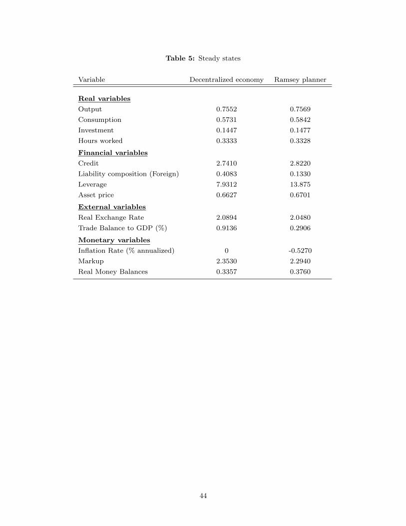
Table 5: Steady states

Variable Decentralized economy Ramsey planner

Real variables

Output 0.7552 0.7569

Consumption 0.5731 0.5842

Investment 0.1447 0.1477

Hours worked 0.3333 0.3328

Financial variables

Credit 2.7410 2.8220

Liability composition (Foreign) 0.4083 0.1330

Leverage 7.9312 13.875

Asset price 0.6627 0.6701

External variables

Real Exchange Rate 2.0894 2.0480

Trade Balance to GDP (%) 0.9136 0.2906

Monetary variables

Inflation Rate (% annualized) 0 -0.5270

Markup 2.3530 2.2940

Real Money Balances 0.3357 0.3760

44

Table 6: Relative volatilities

Variable Decentralized economy Ramsey planner

Real variables

Output 1.00 1.00

Consumption 0.70 0.70

Investment 4.93 5.06

Hours Worked 2.09 1.32

Financial variables

Credit 2.25 2.97

Liability Composition (Foreign) 1.95 4.42

Loan-domestic deposit spread 0.20 0.18

Loan-foreign deposit spread 0.37 0.14

Leverage 12.43 2.51

Net Worth 14.13 3.11

External variables

Real Exchange Rate 5.95 2.21

CA Balance to GDP 1.05 0.27

Trade Balance to GDP 0.33 0.32

Monetary variables

Inflation Rate 0.34 0.11

Policy Rate 0.11 0.25

Markup 7.97 5.13

45

Table 7: Optimal simple policy rules under external shocks

Country risk premium ρrn ϕπ ϕy ϕf ρrr ϕrr σrn σπ σspread σRER σq CEV(%)a

Optimized Taylor rules (TR)

Standard (without smoothing) - 1.0010 0 - - - 0.7878 1.4067 0.2464 7.3900 1.2141 4.5849

Standard (with smoothing) 0.9950 1.0010 0 - - - 0.0032 0.4044 0.1129 6.0891 1.0429 0.2912

Optimized augmented TR

Credit 0.6396 1.0010 1.0714 -0.4286 - - 0.5565 0.2489 0.8716 6.7310 5.0710 0.0096

Asset price 0.6396 1.4294 0.6429 -1.0714 - - 3.1285 0.6709 1.3206 7.4468 10.2921 0.0021

Credit spread 0.9239 1.4294 0.4286 -2.1429 - - 0.5134 1.1540 0.0265 6.9217 0.4592 0.0026

Real exchange rate 0.9950 1.0010 0.4286 3.0000 - - 0.1381 0.1837 0.8079 5.8538 5.0637 0.0015

Optimized TR and RRR 0.3554 1.1438 2.3571 - 0.4264 -2.5714 0.2322 0.5677 0.0281 6.2455 0.9535 0.0006

Ramsey policy - - - - - - 0.3610 0.0668 0.2211 3.3243 5.0007 0

U.S. interest rate ρrn ϕπ ϕy ϕf ρrr ϕrr σrn σπ σspread σRER σq CEV(%)

Optimized Taylor rules (TR)

Standard (without smoothing) - 1.0010 0 - - - 0.3479 0.6212 0.1072 2.8912 0.5296 2.3948

Standard (with smoothing) 0.9950 1.0010 0 - - - 0.013 0.1622 0.0427 2.3181 0.4070 1.7815

Optimized augmented TR

Credit 0.4975 1.0010 2.3571 -1.0714 - - 0.8100 0.2149 0.4128 1.6112 2.6099 0.0011

Asset price 0.2132 3.0000 2.1429 -2.1429 - - 2.6984 0.1644 0.4259 3.2054 3.3204 0.0009

Credit spread 0.9239 1.0010 3.0000 -3.0000 - - 0.2784 0.5925 0.0123 2.7718 0.2092 0.0050

Real exchange rate 0.1421 1.2866 1.0714 1.2857 - - 1.3936 0.3017 2.0838 4.1775 12.566 0.0025

U.S. interest rate 0.7818 1.0010 0 2.5714 - - 0.9770 3.3691 2.2266 3.0112 13.368 0.0121

Optimized TR and RRR 0.4264 1.1438 1.9286 - 0.2843 -2.7857 0.0821 0.2120 0.0161 2.3449 0.3698 0.0004

Ramsey policy - - - - - - 0.1333 0.0308 0.0901 1.3029 1.9737 0

Export demand ρrn ϕπ ϕy ϕf ρrr ϕrr σrn σπ σspread σRER σq CEV(%)

Optimized Taylor rules (TR)

Standard (without smoothing) - 3.0000 0.6429 - - - 0.0028 0.0084 0.0153 0.1041 0.0323 2.0777

Standard (with smoothing) 0.9950 1.0010 0 - - - 0.0001 0.0049 0.0139 0.1058 0.0340 2.0769

Optimized augmented TR

Credit 0.9950 3.0000 0.6429 -2.7857 - - 0.0298 0.2260 0.2939 0.5507 1.8000 0.0794

Asset price 0.2843 1.0010 0.4286 -2.1429 - - 0.9875 0.1947 0.2077 1.7078 1.2732 0.0047

Credit spread 0.0711 1.0010 1.7143 -2.5714 - - 0.4595 0.7643 0.0014 0.9428 0.2299 0.0001

Real exchange rate 0.2843 1.1438 0 1.7143 - - 0.1597 0.0753 0.2641 0.2027 1.7710 0.0063

Optimized TR and RRR 0.9950 1.0010 1.7143 - 0.5686 -3.0000 0.0068 0.1101 0.0573 0.1529 0.8350 0.0021

Ramsey policy - - - - - - 0.0062 0.0042 0.0140 0.0610 0.0564 0

aThe reported welfare figures include both long-run and dynamic costs.

46

Table 8: Optimal simple policy rules under all shocks

All shocks ρrn ϕπ ϕy ϕf ρrr ϕrr σrn σπ σspread σRER σq CEV(%)a

Optimized Taylor rules (TR)

Standard (without smoothing) - 1.0010 0 - - - 0.9424 1.6829 0.2734 7.9497 1.3517 6.0616

Standard (with smoothing) 0.9239 1.0010 0 - - - 0.0614 0.5532 0.1757 6.5809 1.3472 2.1345

Optimized Augmented TR

Credit 0.9239 1.0010 1.7143 -0.6429 - - 0.2401 0.3229 0.7744 6.4310 4.7299 0.0450

Asset price 0.8529 2.4289 1.9286 -2.7857 - - 3.8831 0.9414 0.8868 10.716 11.529 0.0013

Credit spread 0.9950 1.0010 2.7857 -1.500 - - 0.0908 0.5682 0.0579 6.7198 0.8986 0.0027

Real exchange rate 0.9950 1.0010 0.4286 2.7857 - - 0.1391 0.3735 0.8674 6.3262 5.3979 0.0093

U.S. interest rate 0.9239 1.0010 0 0.2143 - - 0.0593 0.5302 0.2976 6.5545 1.9367 0.1332

Optimized TR and RRR 0.5686 1.4294 2.1429 - 0.3554 -1.7143 0.4565 0.9267 0.3220 6.6794 1.9311 0.0040

Ramsey policy - - - - - - 0.4460 0.1861 0.2472 3.8810 5.4933 0

aThe reported welfare figures include both long-run and dynamic costs.

47

Online Appendix for “External Shocks, Banks and Optimal

Monetary Policy: A Recipe for Emerging Market Central Banks”.

Not Intended for Publication.1

Yasin Mimir2 Enes Sunel3

September 28, 2017

1We would like to thank Leonardo Gambacorta, Nobuhiro Kiyotaki, Giovanni Lombardo, Hyun Song Shin, PhilipTurner, the seminar participants at the Bank for International Settlements, the Central Bank of Turkey, NorgesBank, the Georgetown Center for Economic Research Biennial Conference 2015, the CBRT-BOE Joint Workshop2015 on “The International Monetary and Financial System – long-term challenges, short-term solutions”, the 21stInternational Conference on Computing in Economics and Finance, the 11th World Congress of the EconometricSociety, and the 47th Money, Macro and Finance Research Group Annual conference for their helpful comments andsuggestions. This paper circulated earlier under the title “External Shocks, Banks and Optimal Monetary Policy in anOpen Economy”. Yasin Mimir completed this project while visiting the Bank for International Settlements under theCentral Bank Research Fellowship programme. The views expressed in this paper are those of the authors only anddo not necessarily reflect the views of Norges Bank or of the Bank for International Settlements (BIS). The usualdisclaimer applies.

2Corresponding author. Norges Bank, Monetary Policy Department, Bankplassen 2, 0151 Oslo, Norway, Phone:+4722316811, yasin.mimir@norges-bank.no, Personal homepage: http://www.yasinmimir.com

3Sunel & Sunel Law Firm. Soganlik Yeni Mah., Uprise Elite Residence 234, Kartal, 34880 Istanbul, Turkey, Phone:+905334451145, email: enessunel@gmail.com, Personal homepage: https://sites.google.com/site/enessunel/

i

A Model derivations

A.1 Households

There is a large number of infinitely-lived identical households, who derive utility from consump-

tion ct, leisure (1− ht), and real money balances MtPt

. The consumption good is a constant-elasticity-

of-substitution (CES) aggregate of domestically produced and imported tradable goods as in Galı

and Monacelli (2005) and Gertler et al. (2007),

ct =[ω

1γ (cHt )

γ−1γ + (1− ω)

1γ (cFt )

γ−1γ

] γγ−1

, (A.1)

where γ > 0 is the elasticity of substitution between home and foreign goods, and 0 < ω < 1 is the

relative weight of home goods in the consumption basket, capturing the degree of home bias in

household preferences. Let PHt and PFt represent domestic currency denominated prices of home

and foreign goods, which are aggregates of a continuum of differentiated home and foreign good

varieties, respectively.

The expenditure minimization problem of households

mincHt ,c

Ft

Ptct − PHt cHt − PFt cFt

subject to (A.1) yields the demand curves cHt = ω(PHtPt

)−γct and cFt = (1−ω)

(PFtPt

)−γct, for home

and foreign goods, respectively.

The final demand for home consumption good cHt , is an aggregate of a continuum of varieties

of intermediate home goods along the [0,1] interval. That is, cHt =[∫ 1

0 (cHit )1− 1ε di] 1

1− 1ε , where each

variety is indexed by i, and ε is the elasticity of substitution between these varieties. For any given

level of demand for the composite home good cHt , the demand for each variety i solves the problem

of minimizing total home goods expenditures,∫ 1

0 PHit c

Hit di subject to the aggregation constraint,

where PHit is the nominal price of variety i. The solution to this problem yields the optimal demand

for cHit , which satisfies

cHit =

(PHitPHt

)−εcHt ,

with the aggregate home good price index PHt being

PHt =

[∫ 1

0(PHit )1−εdi

] 11−ε

.

Therefore, the expenditure minimization problem of households subject to the consumption

aggregator (A.1) produces the domestic consumer price index (CPI),

Pt =[ω(PHt )1−γ + (1− ω)(PFt )1−γ

] 11−γ

(A.2)

i

and the condition that determines the optimal demand frontier for home and foreign goods,

cHtcFt

=ω

1− ω

(PHtPFt

)−γ. (A.3)

We assume that each household is composed of a worker and a banker who perfectly insure

each other. Workers consume the consumption bundle and supply labor ht. They also save in local

currency assets which are deposited within financial intermediaries owned by the banker members of

other households.1 The balance of these deposits is denoted by Bt+1, which promises to pay a net

nominal risk-free rate rnt in the next period. There are no interbank frictions, hence rnt coincides

with the policy rate of the central bank. Furthermore, the borrowing contract is real in the sense

that the risk-free rate is determined based on the expected inflation. By assumption, households

cannot directly save in productive capital, and only banker members of households are able to

borrow in foreign currency.

Preferences of households over consumption, leisure, and real balances are represented by the

lifetime utility function

E0

∞∑t=0

βtU

(ct, ht,

Mt

Pt

), (A.4)

where U is a CRRA type period utility function given by

U

(ct, ht,

Mt

Pt

)=

[(ct − hcct−1)1−σ − 1

1− σ− χ

1 + ξh1+ξt + υ log

(Mt

Pt

)]. (A.5)

Et is the mathematical expectation operator conditional on the information set available at t,

β ∈ (0, 1) is the subjective discount rate, σ > 0 is the inverse of the intertemporal elasticity of

substitution, hc ∈ [0, 1) governs the degree of habit formation, χ is the utility weight of labor, and

ξ > 0 determines the Frisch elasticity of labor supply. We also assume that the natural logarithm of

real money balances provides utility in an additively separable fashion with the utility weight υ.2

Households face the flow budget constraint,

ct +Bt+1

Pt+Mt

Pt=

Wt

Ptht +

(1 + rnt−1)BtPt

+Mt−1

Pt+ Πt −

TtPt. (A.6)

On the right hand side are the real wage income WtPtht, real balances of the domestic currency

interest bearing assets at the beginning of period t BtPt

, and real money balances at the beginning

of period t Mt−1

Pt. Πt denotes real profits remitted from firms owned by the households (banks,

intermediate home goods producers, and capital goods producers). Tt represents nominal lump-

sum taxes collected by the government. On the left hand side are the outlays for consumption

expenditures and asset demands.

1This assumption is useful in making the agency problem that we introduce in Section 3.2 more realistic.2The logarithmic utility used for real money balances does not matter for real allocations as it enters into the

utility function in an additively separable fashion and money does not appear in any optimality condition except theconsumption-money optimality condition.

ii

Households choose ct, ht, Bt+1, and Mt to maximize preferences in (A.5) subject to (A.6) and

standard transversality conditions imposed on asset demands Bt+1, and Mt. The first order

conditions of the utility maximization problem of households are given by

ϕt = (ct − hcct−1)−σ − βhcEt (ct+1 − hcct)−σ , (A.7)

Wt

Pt=χhξtϕt

, (A.8)

ϕt = βEt

[ϕt+1(1 + rnt)

PtPt+1

], (A.9)

υ

Mt/Pt= βEt

[ϕt+1rnt

PtPt+1

]. (A.10)

Equation (A.7) defines the Lagrange multiplier ϕt as the marginal utility of consuming an additional

unit of income. Equation (A.8) equates marginal disutility of labor to the shadow value of real wages.

Finally, equations (A.9) and (A.10) represent the Euler equations for bonds, the consumption-savings

margin, and money demand, respectively.

First order conditions (A.7) and (A.9) that come out of the utility maximization problem can

be combined to obtain the consumption-savings optimality condition,

(ct − hcct−1)−σ−βhcEt (ct+1 − hcct)−σ = βEt

[{(ct+1 − hcct)−σ − βhc (ct+2 − hcct+1)−σ

} (1 + rnt+1)PtPt+1

].

The consumption-money optimality condition,

υ/mt

ϕt=

rnt1 + rnt

.

on the other hand, might be derived by combining first order conditions (A.9) and (A.10) with mt

denoting real balances held by consumers.

A.2 Banks’ net worth maximization

Bankers solve the following value maximization problem,

Vjt = maxljt+i,b∗jt+1+i

Et

∞∑i=0

(1− θ)θiΛt,t+1+i njt+1+i

= maxljt+i,b∗jt+1+i

Et

∞∑i=0

(1− θ)θiΛt,t+1+i

( [Rkt+1+i − Rt+1+i

]qt+iljt+i

+[Rt+1+i −R∗t+1+i

]b∗jt+1+i + Rt+1+injt+i

).

iii

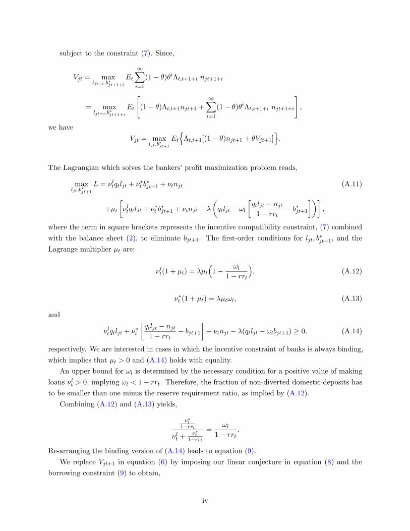
subject to the constraint (7). Since,

Vjt = maxljt+i,b∗jt+1+i

Et

∞∑i=0

(1− θ)θiΛt,t+1+i njt+1+i

= maxljt+i,b∗jt+1+i

Et

[(1− θ)Λt,t+1njt+1 +

∞∑i=1

(1− θ)θiΛt,t+1+i njt+1+i

],

we have

Vjt = maxljt,b∗jt+1

Et

{Λt,t+1[(1− θ)njt+1 + θVjt+1]

}.

The Lagrangian which solves the bankers’ profit maximization problem reads,

maxljt,b∗jt+1

L = νltqtljt + ν∗t b∗jt+1 + νtnjt (A.11)

+µt

[νltqtljt + ν∗t b

∗jt+1 + νtnjt − λ

(qtljt − ωl

[qtljt − njt

1− rrt− b∗jt+1

])],

where the term in square brackets represents the incentive compatibility constraint, (7) combined

with the balance sheet (2), to eliminate bjt+1. The first-order conditions for ljt, b∗jt+1, and the

Lagrange multiplier µt are:

νlt(1 + µt) = λµt

(1− ωl

1− rrt

), (A.12)

ν∗t (1 + µt) = λµtωl, (A.13)

and

νltqtljt + ν∗t

[qtljt − njt

1− rrt− bjt+1

]+ νtnjt − λ(qtljt − ωlbjt+1) ≥ 0, (A.14)

respectively. We are interested in cases in which the incentive constraint of banks is always binding,

which implies that µt > 0 and (A.14) holds with equality.

An upper bound for ωl is determined by the necessary condition for a positive value of making

loans νlt > 0, implying ωl < 1− rrt. Therefore, the fraction of non-diverted domestic deposits has

to be smaller than one minus the reserve requirement ratio, as implied by (A.12).

Combining (A.12) and (A.13) yields,

ν∗t1−rrt

νlt +ν∗t

1−rrt

=ωl

1− rrt.

Re-arranging the binding version of (A.14) leads to equation (9).

We replace Vjt+1 in equation (6) by imposing our linear conjecture in equation (8) and the

borrowing constraint (9) to obtain,

iv

Vjt = Et

{Ξt,t+1njt+1

}, (A.15)

where Vjt stands for the optimized value.

Replacing the left-hand side to verify our linear conjecture on bankers’ value (8) and using

equation (5), we obtain the definition of the augmented stochastic discount factor Ξt,t+1 = Λt,t+1

[1−

θ+ θ(ζt+1κt+1 + νt+1−

ν∗t+1

1−rrt+1

)]and find that νlt, νt, and ν∗t should consecutively satisfy equations

(10), (11) and (12) in the main text.

Surviving bankers’ net worth net+1 is derived as described in the main text and is equal to

net+1 = θ

([Rkt+1 − Rt+1 +

Rt+1 −R∗t+1

1− rrt

]κt −

[Rt+1 −R∗t+1

1− rrt

]+ Rt+1

)nt

+

([Rkt+1 − Rt+1 +

Rt+1 −R∗t+1

1− rrt

]ωl −

[Rt+1 −R∗t+1

1− rrt

])bt+1.

A.3 Capital producers

Capital producers play a profound role in the model since variations in the price of capital

drives the financial accelerator. We assume that capital producers operate in a perfectly competitive

market, purchase investment goods and transform them into new capital. They also repair the

depreciated capital that they buy from the intermediate goods producing firms. At the end of

period t, they sell both newly produced and repaired capital to the intermediate goods firms at the

unit price of qt. Intermediate goods firms use this new capital for production at time t+ 1. Capital

producers are owned by households and return any earned profits to their owners. We also assume

that they incur investment adjustment costs while producing new capital, given by the following

quadratic function of the investment growth

Φ

(itit−1

)=

Ψ

2

[itit−1− 1

]2

.

Capital producers use an investment good that is composed of home and foreign final goods in

order to repair the depreciated capital and to produce new capital goods

it =[ω

1γii (iHt )

γi−1

γi + (1− ωi)1γi (iFt )

γi−1

γi

] γiγi−1

,

where ωi governs the relative weight of home input in the investment composite good and γi measures

the elasticity of substitution between home and foreign inputs. Capital producers choose the optimal

mix of home and foreign inputs according to the intratemporal first order condition

iHtiFt

=ωi

1− ωi

(PHtPFt

)−γi.

The resulting aggregate investment price index P It is given by

v

P It =[ωi(P

Ht )1−γi + (1− ωi)(PFt )1−γi

] 11−γi .

Capital producers require it units of investment good at a unit price ofP ItPt

and incur investment

adjustment costs Φ(

itit−1

)per unit of investment to produce new capital goods it and repair the

depreciated capital, which will be sold at the price qt. Therefore, a capital producer makes an

investment decision to maximize its discounted profits represented by

maxit+i

∞∑i=0

E0

[Λt,t+1+i

(qt+iit+i − Φ

(it+iit+i−1

)qt+iit+i −

P It+iPt+i

it+i

)]. (A.16)

The optimality condition with respect to it produces the following Q-investment relation for capital

goods

P ItPt

= qt

[1− Φ

(itit−1

)− Φ

′(

itit−1

)itit−1

]+ Et

[Λt,t+1qt+1Φ

′(it+1

it

)(it+1

it

)2].

Finally, the aggregate physical capital stock of the economy evolves according to

kt+1 = (1− δt)kt +

[1− Φ

(itit−1

)]it, (A.17)

with δt being the endogenous depreciation rate of capital determined by the utilization choice of

intermediate goods producers.

A.4 Final goods producers

Finished goods producers combine different varieties yt(i), that sell at the monopolistically

determined price PHt (i), into a final good that sells at the competitive price PHt , according to the

constant returns-to-scale technology,

yHt =

[∫ 1

0yHt (i)1− 1

ε di

] 1

1− 1ε.

The profit maximization problem of final goods producers are represented by

maxyHt (i)

PHt

[∫ 1

0yHt (i)1− 1

ε di

] 1

1− 1ε −

[∫ 1

0PHt (i)yHt (i)di

]. (A.18)

The profit maximization problem, combined with the zero profit condition implies that the

optimal variety demand is,

yHt (i) =

(PHt (i)

PHt

)−εyHt ,

with, PHt (i) and PHt satisfying,

vi

PHt =

[∫ 1

0PHt (i)1−εdi

] 11−ε

.

We assume that imported intermediate good varieties are repackaged via a similar technology with

the same elasticity of substitution between varieties as in domestic final good production. Therefore,

yFt (i) =(PFt (i)

PFt

)−εyFt and PFt =

[∫ 10 P

Ft (i)1−εdi

] 11−ε

hold for imported intermediate goods.

A.5 Intermediate goods producers

There is a large number of intermediate goods producers indexed by i, who produce variety yt(i)

using the constant returns-to-scale production technology,

yt(i) = At

(ut(i)kt(i)

)αht(i)

1−α.

As shown in the production function, firms choose the level of capital and labor used in production,

as well as the utilization rate of the capital stock. At represents the aggregate productivity level

and follows an autoregressive process given by

ln(At+1) = ρA ln(At) + εAt+1,

with zero mean and constant variance innovations εAt+1.

Part of yt(i) is sold in the domestic market as yHt (i), in which the producer i operates as a

monopolistically competitor. Accordingly, the nominal sales price PHt (i) is chosen by the firm to

meet the aggregate domestic demand for its variety,

yHt (i) =

(PHt (i)

PHt

)−εyHt ,

which depends on the aggregate home output yHt . Apart from incurring nominal marginal costs of

production MCt, these firms additionally face Rotemberg (1982)-type quadratic menu costs of price

adjustment in the form of

PtϕH

2

[PHt (i)

PHt−1(i)− 1

]2

.

These costs are denoted in nominal terms with ϕH capturing the intensity of the price rigidity.

Domestic intermediate goods producers choose their nominal price level to maximize the present

discounted real profits. We confine our interest to symmetric equilibrium, in which all intermediate

producers choose the same price level that is, PHt (i) = PHt ∀i .

Domestic intermediate goods producers’ profit maximization problem can be represented as

follows:

vii

maxPHt (i)

Et

∞∑j=0

Λt,t+j

[DHt+j(i)

Pt+j

](A.19)

subject to the nominal profit function

DHt+j(i) = PHt+j(i)y

Ht+j(i) + St+jP

H∗t+jc

H∗t+j(i)−MCt+jyt+j(i)− Pt+j

ϕH

2

[PHt+j(i)

PHt+j−1(i)− 1

]2

, (A.20)

and the demand function yHt (i) =(PHt (i)

PHt

)−εyHt . Since households own these firms, any profits are

remitted to consumers and future streams of real profits are discounted by the stochastic discount

factor of consumers, accordingly. Notice that the sequences of the nominal exchange rate and export

prices in foreign currency {St+j , PH∗t+j}∞j=0 are taken exogenously by the firm, since it acts as a price

taker in the export market. The first-order condition to this problem becomes,

(ε− 1)

(PHt (i)

PHt

)−εyHtPt

= ε

(PHt (i)

PHt

)−ε−1

MCtyHtPtPHt

− ϕH[PHt (i)

PHt−1(i)− 1

]1

PHt−1(i)

+ ϕHEt

{Λt,t+1

[PHt+1(i)

PHt (i)− 1

]PHt+1(i)

PHt (i)2

}. (A.21)

Imposing the symmetric equilibrium condition to the first order condition of the profit maxi-

mization problem and using the definitions rmct = MCtPt

, πHt =PHtPHt−1

, and pHt =PHtPt

yield

pHt =ε

ε− 1rmct −

ϕH

ε− 1

πHt (πHt − 1)

yHt+

ϕH

ε− 1Et

{Λt,t+1

πHt+1(πHt+1 − 1)

yHt

}. (A.22)

Notice that even if prices are flexible, that is ϕH = 0, the monopolistic nature of the intermediate

goods market implies that the optimal sales price reflects a markup over the marginal cost that is,

PHt = εε−1MCt.

The remaining part of the intermediate goods is exported as cH∗t (i) in the foreign market, where

the producer is a price taker. To capture the foreign demand, we follow Gertler et al. (2007) and

impose an autoregressive exogenous export demand function in the form of

cH∗t =

[(PH∗t

P ∗t

)−Γ

y∗t

]νH(cH∗t−1)1−νH ,

which positively depends on foreign output that follows an autoregressive exogeneous process,

ln(y∗t+1) = ρy∗

ln(y∗t ) + εy∗

t+1,

viii

with zero mean and constant variance innovations. The innovations to the foreign output process are

perceived as export demand shocks by the domestic economy. For tractability, we further assume

that the small open economy takes PH∗t = P ∗t = 1 as given.

Imported intermediate goods are purchased by a continuum of producers that are analogous to

the domestic producers except that these firms face exogenous import prices as their marginal cost.

In other words, the law of one price holds for the import prices, so that MCFt = StPF∗t . Since these

firms also face quadratic price adjustment costs, the domestic price of imported intermediate goods

is determined as,

pFt =ε

ε− 1st −

ϕF

ε− 1

πFt (πFt − 1)

yFt+

ϕF

ε− 1Et

{Λt,t+1

πFt+1(πFt+1 − 1)

yFt

}, (A.23)

with pFt =PFtPt

, st =StPF∗tPt

, and PF∗t = 1 ∀t is taken exogenously by the small open economy.

For a given sales price, optimal factor demands and utilization of capital are determined by the

solution to a symmetric cost minimization problem, where the cost function shall reflect the capital

gains from market valuation of firm capital and resources that are devoted to the repair of the worn

out part of it. Consequently, firms minimize

minut,kt,ht

qt−1rktkt − (qt − qt−1)kt + pIt δ(ut)kt + wtht + rmct

[yt −At

(utkt

)αh1−αt

](A.24)

subject to the endogeneous depreciation rate function,

δ(ut) = δ +d

1 + %u1+%t , (A.25)

with δ, d, % > 0. The first order conditions to this problem govern factor demands and the optimal

utilization choice as,

pIt δ′(ut)kt = α

( ytut

)rmct, (A.26)

Rkt =α(ytkt

)rmct − pIt δ(ut) + qt

qt−1, (A.27)

and

wt = (1− α)( ytht

)rmct. (A.28)

A.6 Resource constraints

The resource constraint for home goods equates domestic production to the sum of domestic

and external demand for home goods and the real domestic price adjustment costs, so that

ix

yHt = cHt + cH∗t + iHt + gHt yHt +

(pHt

)−γ ϕH2

(πtpHtpHt−1

− 1

)2

. (A.29)

A similar market clearing condition holds for the domestic consumption of the imported goods, that

is,

yFt = cFt + iFt +(pFt

)−γ ϕF2

(πt

pFtpFt−1

− 1)2. (A.30)

The balance of payments vis-a-vis the rest of the world defines the trade balance as a function of

net foreign assets

R∗t b∗t − b∗t+1 = cH∗t − yFt . (A.31)

Finally, the national income identity that reflects investment adjustment costs built in capital

accumulation condition (A.17) would read,

yt = yHt − yFt . (A.32)

A.7 Definition of competitive equilibrium

A competitive equilibrium is defined by sequences of prices{pHt , p

Ft , p

It , πt, wt, qt, st, Rkt+1,

Rt+1, R∗t+1

}∞t=0

, government policies {rnt, rrt,M0t, Tt}∞t=0, allocations{cHt , c

Ft , ct, ht,mt, bt+1, b

∗t+1, ϕt,

lt, nt, κt, νlt, ν∗t , νt, it, i

Ht , i

Ft , kt+1, y

Ht , y

Ft , yt, ut, rmct, c

H∗t , DH

t ,Πt, δt

}∞t=0

, initial conditions, b0, b∗0, k0,

m−, n0 and exogenous processes{At, g

Ht , ψt, r

∗nt, y

∗t

}∞t=0

such that;

i) Given exogenous processes, initial conditions, government policy, and prices; the allocations

solve the utility maximization problem of households (A.5)-(A.6), the net worth maximization

problem of bankers (6)-(7), and the profit maximization problems of capital producers (A.16),

final goods producers (A.18), and intermediate goods producers (A.19)-(A.20) and (A.24)-

(A.25).

ii) Home and foreign goods, physical capital, investment, security claims, domestic deposits,

money, and labor markets clear. The balance of payments and GDP identities (A.31) and

(A.32) hold.

B Impulse responses under domestic and other external shocks

This section presents the impulse responses of real, financial and external variables under the

productivity, government spending, U.S. policy rate and export demand shocks. For brevity, we do

not explain the dynamics of model variables under each shock in detail. We note that most of the

endogenous variables and the policy instruments respond to each shock in a fairly standard way,

which were already extensively studied in the previous literature. In this section, we also report

one-quarter and one-year ahead variance decomposition results.

x

Fig

ure

B.1

:Im

pu

lse

resp

onse

fun

ctio

ns

dri

ven

by

1s.

d.

incr

ease

inp

rod

uct

ivit

y

05

1015

20−

0.2

−0.

10

0.1

0.2

Cur

rent

acc

ount

bal

ance

−to

−ou

tput

%Ch.

05

1015

200

0.2

0.4

0.6

0.8

Rea

l exc

hang

e ra

te

05

1015

20−

0.10

0.1

0.2

0.3

0.4

%Ch.

Nom

inal

dep

reci

atio

n ra

te

05

1015

20−

1.5

−1

−0.

50S

hare

of f

orei

gn d

ebt

05

1015

20−

0.8

−0.

6

−0.

4

−0.

20

0.2

Ann. % Pt. Ch.

CP

I inf

latio

n

05

1015

20−

30

−20

−100

Ann. Bs. Pt. Ch.

Pol

icy

rate

05

1015

200

0.1

0.2

0.3

0.4

0.5

Out

put

%Ch.

05

1015

200

0.050.

1

0.150.

2

0.25

Con

sum

ptio

n

05

1015

20−

0.50

0.51

Inve

stm

ent

05

1015

200

0.2

0.4

0.6

0.8

Cre

dit

%Ch.

05

1015

20−

2

−1.

5

−1

−0.

50B

ank

net w

orth

05

1015

20−

0.2

−0.

10

0.1

0.2

Ass

et p

rice

05

1015

20−

15

−10−

50510Lo

an−

fore

ign

depo

sits

spr

ead

Ann. Bs. Pt. Ch.

Qua

rter

s0

510

1520

−2

−1.

5

−1

−0.

50

0.5

Loan

−do

mes

tic d

epos

its s

prea

d

Qua

rter

s0

510

1520

−30

−20

−1001020

Rea

l int

eres

t rat

e

Qua

rter

s0

510

1520

0123P

rodu

ctiv

ity

Qua

rter

s

xi

Fig

ure

B.2

:Im

pu

lse

resp

onse

fun

ctio

ns

dri

ven

by

1s.

d.

incr

ease

ingo

vern

men

tsp

end

ing

05

1015

20−

20

−15

−10−

505x

10−

3C

urre

nt a

ccou

nt b

alan

ce−

to−

outp

ut

%Ch.

05

1015

20−

0.08

−0.

06

−0.

04

−0.

020

0.02

Rea

l exc

hang

e ra

te

05

1015

20−

0.06

−0.

04

−0.

020

0.02

%Ch.

Nom

inal

dep

reci

atio

n ra

te

05

1015

200

0.050.

1

0.150.

2S

hare

of f

orei

gn d

ebt

05

1015

20−

0.020

0.02

0.04

0.06

0.08

Ann. % Pt. Ch.

CP

I inf

latio

n

05

1015

200

0.51

1.52

Ann. Bs. Pt. Ch.

Pol

icy

rate

05

1015

20−

0.20

0.2

0.4

0.6

Out

put

%Ch.

05

1015

20−

0.02

−0.

015

−0.

01

−0.

0050

Con

sum

ptio

n

05

1015

20−

0.02

−0.

010

0.01

0.02

Inve

stm

ent

05

1015

20−

0.06

−0.

04

−0.

020C

redi

t

%Ch.

05

1015

200

0.1

0.2

0.3

0.4

Ban

k ne

t wor

th

05

1015

20−

505101520x

10−

3A

sset

pric

e

05

1015

20−

3

−2

−10

Loan

−fo

reig

n de

posi

ts s

prea

d

Ann. Bs. Pt. Ch.

Qua

rter

s0

510

1520

−0.

2

−0.

15

−0.

1

−0.

050

0.05

Loan

−do

mes

tic d

epos

its s

prea

d

Qua

rter

s0

510

1520

−10123

Rea

l int

eres

t rat

e

Qua

rter

s0

510

1520

−20246

Gov

ernm

ent s

pend

ing

Qua

rter

s

xii

Fig

ure

B.3

:Im

pu

lse

resp

onse

fun

ctio

ns

dri

ven

by

40an

nu

aliz

edb

asis

poi

nts

incr

ease

inth

eU

.S.

poli

cyra

te

05

1015

200

0.1

0.2

0.3

0.4

Cur

rent

acc

ount

bal

ance

−to

−ou

tput

%Ch.

05

1015

200

0.51

1.52

Rea

l exc

hang

e ra

te

05

1015

20−

0.50

0.51

1.52

%Ch.

Nom

inal

dep

reci

atio

n ra

te

05

1015

20−

1.5

−1

−0.

50

0.5

Sha

re o

f for

eign

deb

t

05

1015

200

0.1

0.2

0.3

0.4

Ann. % Pt. Ch.

CP

I inf

latio

n

05

1015

2005101520

Ann. Bs. Pt. Ch.

Pol

icy

rate

05

1015

20−

0.25

−0.

2

−0.

15

−0.

1

−0.

050O

utpu

t

%Ch.

05

1015

20−

0.25

−0.

2

−0.

15

−0.

1

−0.

050C

onsu

mpt

ion

05

1015

20−

1.5

−1

−0.

50In

vest

men

t

05

1015

20−

0.8

−0.

6

−0.

4

−0.

20C

redi

t

%Ch.

05

1015

20−

5

−4

−3

−2

−10

Ban

k ne

t wor

th

05

1015

20−

0.8

−0.

6

−0.

4

−0.

20

0.2

Ass

et p

rice

05

1015

20−

20020406080Lo

an−

fore

ign

depo

sits

spr

ead

Ann. Bs. Pt. Ch.

Qua

rter

s0

510

1520

02468Lo

an−

dom

estic

dep

osits

spr

ead

Qua

rter

s0

510

1520

−20

−1001020

Rea

l int

eres

t rat

e

Qua

rter

s0

510

1520

010203040U

S in

tere

st r

ate

Qua

rter

s

xiii

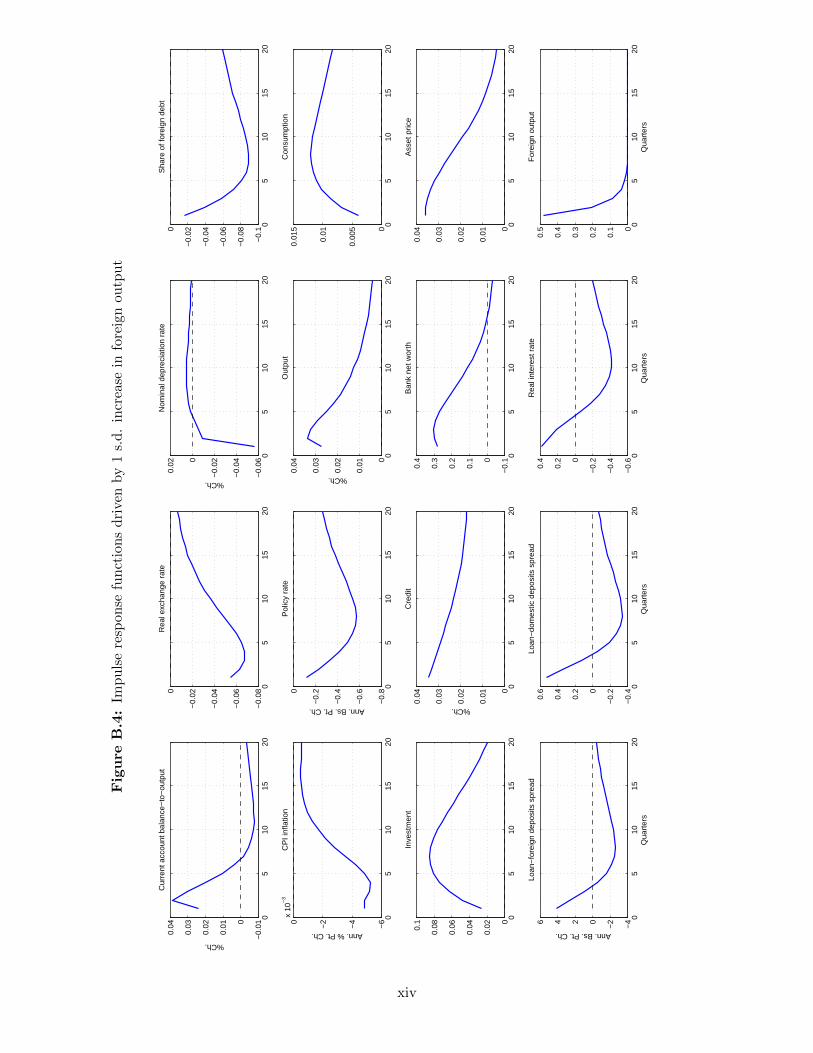
Fig

ure

B.4

:Im

pu

lse

resp

onse

fun

ctio

ns

dri

ven

by

1s.

d.

incr

ease

info

reig

nou

tpu

t

05

1015

20−

0.010

0.01

0.02

0.03

0.04

Cur

rent

acc

ount

bal

ance

−to

−ou

tput

%Ch.

05

1015

20−

0.08

−0.

06

−0.

04

−0.

020R

eal e

xcha

nge

rate

05

1015

20−

0.06

−0.

04

−0.

020

0.02

%Ch.

Nom

inal

dep

reci

atio

n ra

te

05

1015

20−

0.1

−0.

08

−0.

06

−0.

04

−0.

020S

hare

of f

orei

gn d

ebt

05

1015

20−

6

−4

−20

x 10

−3

Ann. % Pt. Ch.

CP

I inf

latio

n

05

1015

20−

0.8

−0.

6

−0.

4

−0.

20

Ann. Bs. Pt. Ch.

Pol

icy

rate

05

1015

200

0.01

0.02

0.03

0.04

Out

put

%Ch.

05

1015

200

0.00

5

0.01

0.01

5C

onsu

mpt

ion

05

1015

200

0.02

0.04

0.06

0.080.

1In

vest

men

t

05

1015

200

0.01

0.02

0.03

0.04

Cre

dit

%Ch.

05

1015

20−

0.10

0.1

0.2

0.3

0.4

Ban

k ne

t wor

th

05

1015

200

0.01

0.02

0.03

0.04

Ass

et p

rice

05

1015

20−

4

−20246

Loan

−fo

reig

n de

posi

ts s

prea

d

Ann. Bs. Pt. Ch.

Qua

rter

s0

510

1520

−0.

4

−0.

20

0.2

0.4

0.6

Loan

−do

mes

tic d

epos

its s

prea

d

Qua

rter

s0

510

1520

−0.

6

−0.

4

−0.

20

0.2

0.4

Rea

l int

eres

t rat

e

Qua

rter

s0

510

1520

0

0.1

0.2

0.3

0.4

0.5

For

eign

out

put

Qua

rter

s

xiv

Table B.1: Variance decomposition in the decentralized economy (%)

One quarter ahead TFP Government spending Country risk premium U.S. interest rate Export demand

Output 16.41 67.89 13.05 2.38 0.27

Consumption 17.69 0.12 69.81 12.36 0.03

Investment 5.11 0.00 80.86 13.98 0.05

Credit 96.45 2.54 0.77 0.12 0.11

Liability composition (foreign) 1.64 0.01 83.97 14.32 0.05

Loan-domestic deposit spread 0.04 0.00 84.50 15.36 0.10

Loan-foreign deposit spread 0.75 0.00 84.70 14.49 0.05

Real exchange rate 1.12 0.01 86.41 12.45 0.01

CA balance to GDP 0.04 0.00 79.93 13.72 6.31

Trade balance to GDP 0.18 0.25 79.87 13.73 5.98

Inflation rate 36.25 0.21 56.00 7.55 0.00

Policy rate 36.25 0.21 56.00 7.55 0.00

One year ahead

Output 37.33 15.59 39.67 7.14 0.27

Consumption 15.98 0.10 71.23 12.66 0.03

Investment 6.17 0.00 79.89 13.90 0.05

Credit 70.40 1.40 23.71 4.19 0.31

Liability composition (foreign) 9.34 0.08 77.57 12.98 0.04

Loan-domestic deposit spread 0.91 0.00 84.48 14.58 0.03

Loan-foreign deposit spread 0.28 0.02 85.06 14.61 0.02

Real exchange rate 1.90 0.02 85.50 12.56 0.02

CA balance to GDP 1.30 0.02 84.33 14.17 0.18

Trade balance to GDP 0.94 0.02 83.12 14.46 1.45

Inflation rate 27.13 0.14 64.14 8.60 0.00

Policy rate 23.32 0.09 67.55 9.05 0.00

C Optimal simple rules under domestic shocks

Table C.1 reports the response coefficients of optimized conventional and augmented Taylor

rules, the absolute volatilities of policy rate, inflation, lending spread over foreign debt and the

real exchange rate under these rules, and the corresponding consumption-equivalent welfare costs

relative to the Ramsey-optimal policy under productivity and government spending shocks.

The optimized Taylor rules with and without smoothing feature no response to output variations

under productivity shocks, which is consistent with the results of Schmitt-Grohe and Uribe (2007)

in a canonical closed-economy New Keynesian model without credit frictions. The optimal simple

rule with smoothing displays a large degree of inertia and a limited response to the CPI inflation.

The latter result is in line with Schmitt-Grohe and Uribe (2007) in the sense that the level of

the response coefficient of inflation plays a limited role for welfare and it matters to the extent

xv

that it affects the determinacy. It is also inline with Monacelli (2005), Faia and Monacelli (2008),

and Monacelli (2013) since open economy features such as home bias and incomplete exchange

rate pass-through may cause the policymaker to deviate from strict domestic markup stabilization

and resort to some degree of exchange rate stabilization. Higher volatilities of inflation and credit

spreads together with a lower volatility of asset prices compared to the Ramsey policy indicate that

these two optimized Taylor rules can only partially stabilize the intratemporal and intertemporal

wedges, explaining the welfare losses associated with these rules.

Under productivity shocks, optimized augmented Taylor rules suggest that a negative response

to credit spreads together with a moderate response to inflation and a strong response to output

deviations achieve the highest welfare possible. In response to 100 basis points increase in credit

spreads, the policy should be reduced by 150 basis points, all else equal. This policy substantially

reduces the volatility of spreads in comparison to that in the Ramsey policy. Moreover, the optimized

augmented Taylor rules that respond to credit, asset prices or the real exchange rate also achieve

a level of welfare very close to that implied by the spread-augmented Taylor rule. Both rules

feature a lower degree of volatility of the real exchange rate in comparison to that in the Ramsey

policy. We also observe that it is optimal to negatively respond to bank credit under productivity

shocks. In addition, comparing volatilities of key variables under these augmented Taylor rules

displays the nature of the policy trade-offs that the central bank faces. For instance, although the

spread-augmented rule features a lower volatility of the credit spreads relative to the Ramsey policy

as can be expected, it displays a much higher volatility in the CPI inflation rate. In addition, the

optimized RER-augmented rule features a lower volatility in the real exchange rate as expected but it

displays much larger variations in the inflation rate and the credit spread against the Ramsey-optimal

policy.

Optimized augmented Taylor rules under government spending shocks suggest similar results in

general except the following. In response to this domestic demand shock, which pushes inflation

and output in the same direction, the optimal Taylor rules with or without smoothing display a

positive response to output. The best policy on the other hand, is to respond to the RER instead of

credit spreads, noting that the welfare costs implied by either policy rule relative to the Ramsey

policy are quite similar.

xvi

Table C.1: Optimal simple policy rules under domestic shocks

TFP ρrn ϕπ ϕy ϕf ρrr ϕrr σrn σπ σspread σRER σq CEV(%)a

Optimized Taylor rules (TR)

Standard (without smoothing) - 1.5721 0 - - - 0.2701 0.3071 0.0830 0.4714 0.4155 2.2690

Standard (with smoothing) 0.9950 1.0010 0 - - - 0.0015 0.2559 0.1183 0.9274 0.6568 1.3583

Optimized augmented TR

Credit 0.7818 1.2866 2.7857 -1.7143 - - 0.4441 0.4697 0.1008 1.1231 1.0792 0.0010

Asset price 0.4264 3.0000 2.7857 -3.0000 - - 2.9289 0.7777 0.4339 4.5204 3.5392 0.0009

Credit spread 0.9239 1.2866 1.2857 -1.5000 - - 0.2268 0.3903 0.0234 1.3792 0.4942 0.0001

Real exchange rate 0.7107 1.0010 1.9286 2.7857 - - 0.3718 0.4431 0.8391 1.1026 5.2674 0.0014

Optimized TR and RRR 0.1421 2.8572 1.0714 - 0.7107 -2.7857 0.4204 0.5282 14.5650 12.8479 4.3218 0.0008

Ramsey policy - - - - - - 0.2248 0.1703 0.0623 1.5168 1.1261 0

Government spending ρrn ϕπ ϕy ϕf ρrr ϕrr σrn σπ σspread σRER σq CEV(%)

Optimized Taylor rules (TR)

Standard (without smoothing) - 1.0010 0.2143 - - - 0.0725 0.0427 0.0290 0.1186 0.1641 2.0672

Standard (with smoothing) 0.9950 1.0010 0.4286 - - - 0.0009 0.0145 0.0064 0.0949 0.0616 2.0106

Optimized augmented TR

Credit 0.9950 1.1438 1.5000 -0.8571 - - 0.0089 0.2327 0.2649 0.4117 1.7141 0.0332

Asset price 0.9950 2.4289 1.2857 -2.3571 - - 0.0278 0.1991 0.2551 0.4078 1.6741 0.0010

Credit spread 0.3554 1.2866 0.2143 -2.5714 - - 0.3014 0.4829 0.0007 0.6864 0.2662 0.0147

Real exchange rate 0.1421 1.2866 2.3571 -2.7857 - - 0.3445 0.3008 0.4325 1.2370 3.3088 0.0005

Optimized TR and RRR 0.9950 1.1438 0.8571 - 0.2843 -3.0000 0.0040 0.1182 0.0521 0.2786 0.8837 0.0001

Ramsey policy - - - - - - 0.0144 0.0146 0.0060 0.0961 0.0508 0

aThe reported welfare figures include both long-run and dynamic costs.

xvii