Embed Size (px)
Citation preview

MONETARY POLICY AND EXCHANGE RATE PASS-THROUGH
First Draft: July 2001This Draft: June 2004
Joseph E. Gagnon and Jane Ihrig*
Abstract: The pass-through of exchange rate changes into domestic inflation appears to havedeclined in many countries since the 1980s. We develop a theoretical model that attributes thechange in the rate of pass-through to increased emphasis on inflation stabilization by manycentral banks. This hypothesis is tested on twenty industrial countries between 1971 and 2003. We find widespread evidence of a robust and statistically significant link between estimatedrates of pass-through and inflation variability. We also find evidence that observed monetarypolicy behavior may be a factor in the declining rate of pass-through.
Keywords: inflation targeting, Taylor rule, exchange rate pass-throughJEL: E58, F40
* [email protected] (corresponding author, O:202-452-2528, F:202-872-4926) [email protected] (O:202-452-3372, F:202-736-5638); Division of International Finance, Board ofGovernors of the Federal Reserve System, 2000 C Street NW, Washington, DC 20551. Wewould like to thank Sebastien Bradley and Alisa Wilson for invaluable research assistance. Weare also grateful to Neil Ericsson, Ray Fair, Linda Goldberg, Giovanni Olivei, John Rogers, TedTruman, Jonathan Wright, Kei-Mu Yi and participants in workshops at the Federal ReserveBanks of Atlanta and New York and the Division of International Finance for helpful guidanceand comments. The views in this paper are solely the responsibility of the authors and shouldnot be interpreted as reflecting the views of the Board of Governors of the Federal ReserveSystem or of any other person associated with the Federal Reserve System.

Executive Summary
The pass-through of exchange rate changes into domestic inflation appears to have
declined in many countries since the 1980s. Prominent examples include the United Kingdom
and Sweden after 1992 and Brazil in 1999. We develop a theoretical model that attributes the
change in the rate of pass-through to increased emphasis on inflation stabilization by central
banks in these countries. Simply put, when a central bank acts aggressively to stabilize the
domestic inflation rate it tightens policy to offset any inflationary impetus from a rise in import
prices. This policy reaction holds down price increases in other sectors so that overall inflation
remains stable. When agents correctly understand the central bank’s intentions, they are less
likely to try to pass-through cost increases, including those arising from exchange rate
depreciations.
We test this hypothesis on twenty industrial countries between 1971 and 2003. First, we
show that countries with low and stable inflation rates--presumably reflecting central bank
policies--tend to have low estimated rates of pass-through from exchange rates to consumer
prices. Second, we note a decline in both the level and variability of inflation in many countries
over this period. We create two sub-samples, with sample break dates chosen independently for
each country, based on the observed behavior of inflation, previous research on monetary policy
behavior, and official adoption of inflation targets by central banks in some countries. We show
that countries in which either the level or the standard deviation of inflation declined
substantially from the first to the second sub-sample tended to have large declines in estimated
rates of pass-through.
Finally, we test a more direct connection between monetary policy and pass-through. We
estimate Taylor-type monetary policy rules using the forward-looking specification of Clarida,

Gali, and Gertler (1998). In a cross-country regression using the full sample, we find no
statistically significant relationship between estimated exchange rate pass-through and the
estimated monetary policy parameters. However, there is a statistically significant relationship
between changes in estimated pass-through across the two sub-samples and changes in monetary
policy parameters. In particular, pass-through tended to decline the most in countries where
monetary policy shifted strongly toward stabilizing inflation, as evidenced by an increase in the
responsiveness of policy interest rates to expected inflation.

1
I. Introduction
In the 1990s several countries experienced episodes of large real exchange rate
depreciations that did not lead to significant increases in domestic inflation. The experiences of
Sweden and the United Kingdom in 1992 are two widely cited examples. A potential
explanation of this phenomenon is that central banks in these countries have articulated more or
less formally an enhanced commitment to keeping inflation low since at least the beginning of
the 1990s. In such an environment, firms are less keen to pass through fluctuations in their input
prices to output prices both because the central bank applies countervailing pressure to aggregate
demand contemporaneously, and because firms believe that the central bank will be successful in
stabilizing inflation in the future.
This paper proposes that the anti-inflationary actions and credibility of the monetary
authority are important factors behind the reduced pass-through of exchange rate changes into
consumer price inflation. We develop a simple theoretical model that explains how monetary
policy influences inflation expectations and exchange rate pass-through at the macroeconomic
level. In this model, when the monetary authority focuses strongly on stabilizing inflation, there
is less pass-through of exchange rate movements into consumer prices. We then examine the
monetary and inflation experiences of a sample of industrial countries since the early 1970s.
Empirical results indicate a robust and significant link between the rate of pass-through and the
mean and variability of consumer price inflation. Direct tests using estimated monetary policy
rules suggest that as a monetary authority increases its emphasis on fighting inflation it reduces
the rate of pass-through.

1We focus here on studies of pass-through to broad measures of inflation, such as theCPI.
2In a study of pass-through at different stages of the distribution process, McCarthy(2000) finds that eliminating the years prior to 1983 tends to reduce estimated pass-through in asample of industrial countries.
2
Several studies have identified a reduction in exchange rate pass-through in various
countries.1 For example, Cunningham and Haldane (1999) document the low pass-through of
sterling depreciation in 1992-93 as well as the low pass-through of sterling appreciation in 1996-
97. Taylor (2000) discusses the cases of Sweden and the United Kingdom in 1992-93 and Brazil
in 1999. Goldfajn and Werlang (2000) examine episodes of large depreciations in seven
emerging markets and five industrial countries in the 1990s. In all cases, Goldfajn and Werlang
find that pass-through was less than would have been predicted by their empirical model using
data for the 1980s and 1990s. Norambuena (2003) confirms this result for Chile after 1991.
Laflèche (1996-97) discusses the surprisingly low pass-through of the Canadian depreciation of
1992-94 compared with previous pass-through episodes.2 One of the main contributions of our
study is to explicitly compare the evolution of rates of pass-through in a number of countries.
Both Taylor (2000) and the Bank of Canada have conjectured that changes in pass-
through behavior may be due to changes in the orientation of monetary policy. According to the
Bank of Canada’s November 2000 Monetary Policy Report (p. 9) “the low-inflation environment
itself is changing price-setting behavior. When inflation is low, and the central bank’s
commitment to keeping it low is highly credible, firms are less inclined to quickly pass higher
costs on to consumers in the form of higher prices.” Not many studies, however, have tried to
link pass-through to monetary policy empirically. Parsley and Popper (1998) estimate pass-

3Devereux, Engel, and Storgaard (2003) derive a relationship between the currency ofinvoicing and monetary policy which provides a short-run link between monetary policy andpass-through that is complementary to the long-run relationship developed in this paper.
4Choudhri, Faruqee, and Hakura (2002) derive a negative relationship between meanexpected inflation and macro pass-through based on a microeconomic analysis of firm pricingbehavior that does not model the macroeconomic role of monetary policy.
5Freeman and Willis (1995) provide background on the early experiences of the first fourof these five. While there is some evidence from long-term interest rates that the new policyregimes may not have been immediately and fully credible, inflation rates did come down fasterthan almost anyone expected and policy credibility grew with the observed success in fightinginflation.
3
through for U.S. non-durable goods by industry, recognizing the role that policy plays in
determining the observable relationships between exchange rates and prices, and they find
evidence at the industry level that U.S. monetary policy does influence pass-through. Here we
consider twenty industrial countries and focus on the aggregate price index associated with
monetary policy, which is typically the headline consumer price index.
A key contribution of our study is the formal derivation of the linkage between monetary
policy and exchange rate pass-through to consumer prices.3 Using a simple macro model, we
demonstrate that when a monetary authority increases its emphasis on fighting inflation,
specifically through changes in its policy reaction function, the rate of pass-through declines.4
We test our model’s hypothesis on quarterly data from twenty industrial countries
between 1971 and 2000. Five of these countries -- with a history of moderately high inflation --
adopted explicit and relatively low inflation targets as objectives for monetary policy in the early
1990s. In order of formal adoption of the new regimes, these countries are New Zealand,
Canada, the United Kingdom, Sweden, and Australia.5 Because of their striking changes in
policy regimes, these five countries form a natural experiment with which to test for the impact

6Austria, Belgium, Finland, France, Greece, Ireland, Italy, the Netherlands, Portugal, andSpain.
4
of monetary policy on exchange rate pass-through. Ten other countries in our sample6 – many of
which also have histories of moderately high inflation – increased their exchange rate links to
Germany at various points over the past 30 years, culminating in monetary union with Germany
at the end of the sample. Finally, we analyze five other industrial countries (Germany, Japan,
Norway, Switzerland, and the United States) with more or less independent monetary policies
throughout the sample. Although only five of our countries adopted explicit inflation targets,
monetary regimes in the remaining countries may have moved toward adopting implicit inflation
targets.
We estimate the pass-through of exchange rate changes to consumer price inflation in
each of these countries over the entire sample period, to make cross-country comparisons, as
well as for two sub-samples for each country, to examine changes over time. We find that
estimated rates of pass-through vary across countries and that these rates declined in the second
sample period for 18 of our 20 countries. Next, we show that estimated pass-through
coefficients are very significantly correlated with the standard deviation of the inflation rate,
whether examining cross-country levels of pass-through and inflation variability over the entire
sample or looking at changes in each country’s pass-through and changes in inflation variability
over time. Finally, as a more direct test of our theory, we estimate forward-looking Taylor-type
monetary policy rules for these countries and attempt to correlate components of these policy
rules with estimated rates of pass-through. The results suggest that as a monetary authority
increases its emphasis in fighting inflation it reduces the rate of pass-through.

5
We now turn to section II which presents the theoretical model highlighting the link
between monetary policy and pass-through. We test the model’s implications in Section III.
Concluding comments are in Section IV.
II. A Simple Model
This section explores the relationship between exchange rate pass-through and monetary
policy in the context of a simple macro model with rational expectations. Our objective is to
show how the implied correlation between exchange rate changes and inflation depends on the
monetary policy regime. The six equations of our model are as follows, where all variables are
in logarithms except the interest rate:
(1) [ ]y y y e c c i p ut t t t t t t t t= + + − − + − − − +− + +ρ ρ ρ ρ α β1 2 1 1 1 21 1 1( )( ) ( ) ( )* ∆
(2) ( )∆ ∆ ∆c c c y xt t t t t= + − + +− +ρ ρ γ3 1 31 1
(3) ( )p e c c zt t t t t= + + − +φ φ( )* 1
(4) e E e i i rpt t t t t t= − + ++ 1*
(5) rp rp vt t t= +−ρ4 1
(6) ( ) ( )[ ]i i p p y wt t t t t t= + − + − − + +− + +ρ ρ π µ π λ5 1 51 4 4
where α β γ φ µ λ ρ ρ, , , , , , 1 5 0− >

7In this paper, we assume that direct pass-through of exchange rate changes into theimported component of consumer prices is constant. Campa and Goldberg (2002) find someevidence that a more stable macroeconomic environment tends to reduce pass-through to importprices, which would strengthen our theoretical results. They also find that compositional shiftswithin imported goods have tended to reduce pass-through over time. Olivei (2002) also findsevidence that pass-through into U.S. import prices has declined over time. None of thesechanges in pass-through at the import price level are large enough to explain more than a smallfraction of the estimated changes in pass-through at the consumer price level.
6
Equation (1) states that aggregate demand responds positively to the real exchange rate
(defined as exchange-rate adjusted foreign costs relative to domestic costs) and negatively to the
real interest rate, with a demand shock, u. Lagged adjustment is captured by the parameter D1.
A role for geometrically weighted expectations of future real exchange rates and real interest
rates is captured by the parameter D2, giving the equation the form of an Euler equation under
costly adjustment. Equation (2) is an expectations-augmented Phillips curve for domestic cost,
c, similar to those developed by Fuhrer and Moore (1995) and Christiano, Eichenbaum, and
Evans (2001), where x is a domestic supply shock. The consumer price, p, is a weighted average
of import costs and domestic costs plus a markup shock, z, as presented in equation (3).7
Equation (4) is a standard uncovered interest rate parity relation. Expected exchange rate
appreciation equates any difference between domestic and foreign interest rates, except for a risk
premium, rp. The risk premium is driven by shocks, v, with autocorrelation D4 (equation (5)).
Equation (6) is a monetary policy rule in the style of Taylor (1993) and Clarida, Gali, and Gertler
(1998), where B is the target inflation rate, : represents the strength of the monetary authority’s
response to deviations of inflation from its target, 8 is the response to fluctuations of output, and
w is a policy shock. Note that w may also be interpreted as a temporary shock to the inflation
target. We will interpret a regime shift toward “inflation targeting” as some combination of an

8Fair (2001) finds that the estimated value of : nearly doubled in the United States after1982, when policy succeeded in achieving relatively low and stable inflation.
9Inflation targeting has also been associated with a reduction in the mean inflation rate, B,but a permanent shift in the average level of inflation does not by itself affect the correlation ofinflation and exchange rate changes in this model.
10If both foreign and domestic monetary policy properties change in a similar direction,the implications for pass-through derived here will be dampened, but not eliminated. Limitedexperiments with an expanded model that includes a foreign inflation equation and foreignmonetary policy suggest the impact of changes in foreign monetary policy regimes affectsdomestic pass-through, but the size of the effect is substantially smaller than the effect of anequivalent change in domestic policy regime.
7
increase in : and changes in the other parameters that lead to less variance of inflation around its
target.8,9 Woodford (2003) shows that a rule of this form represents an optimal monetary policy
under plausible assumptions. Note that our model is normalized so that equilibrium values of
aggregate demand, the real exchange rate, the risk premium, and the real interest rate are all zero.
The equilibrium value of the inflation rate is B, and the levels of domestic costs, consumer
prices, and the exchange rate will drift over time reflecting the cumulative impact of all past
shocks.
In order to determine the impact of changing monetary policy regimes on exchange rate
pass-through, we employ Monte Carlo techniques for specific parameterizations of the model.
We first assume that p* and i* are exogenous and set to zero for simplicity.10 We also assume
that the shocks, u, x, z, v, and w are independently and normally distributed with no serial
correlation. We then generate realizations of the shocks and solve the model repeatedly to build
up artificial samples of 100 periods each. For each sample, we estimate the rate of pass-through
as the long-run regression coefficient of inflation on the change in the exchange rate with lags
(as in Section III below); then we calculate the average pass-through estimate across 1000 trials

11Pass-through coefficients for the base model using 1000 trials were within 2 percent ofestimates based on 100 trials and 0.2 percent of estimates based on 10,000 trials.
12See, for example, Table 1 in Hooper, Johnson, and Marquez (2000).
8
and report this as the model’s implied rate of pass-through.11 We repeat this process for different
numerical values of the parameters in order to understand the relationship between monetary
policy and pass-through over a wide range of the parameter space.
The first step is to determine base values of the model parameters to be consistent with
the data. The parameter " captures the extent to which real exchange rate movements affect
aggregate demand. This effect can be broken down into three components: 1) the pass-through
of exchange rates into import prices; 2) the elasticity of domestic and foreign import demand
with respect to import prices; and 3) the share of imports and exports in GDP. Goldberg and
Knetter (1997) provide a discussion of the literature on pass-through to import prices. Typically
50 to 100 percent of an exchange rate change is passed through to import prices, with estimates
for U.S. imports at the bottom of this range. Higher rates of pass-through imply a greater effect
of exchange rates on real activity. Trade price elasticities in aggregate data are generally
estimated around or somewhat below unity; a range of 0.5 to 1 appears reasonable.12 Again,
higher elasticities imply more impact of exchange rates on activity. The share of imports in GDP
ranges from around 10 percent in Japan and the United States to over 80 percent in Belgium and
Ireland, with export shares similar to import shares in each country. Combining these three
ranges and adding up the effects through imports and exports yields a range of values for " from
0.05 to 1.6. However, the upper end of this range should be discounted substantially, as
countries with very large trade shares are likely to have relatively low trade price elasticities and

13See, for example, Freedman (1994) and IMF (1996).
9
rates of pass-through into export prices, reflecting the fact that imported inputs are a large share
of the value of exports, thereby damping the effect of the exchange rate on competitiveness. We
choose a base value of "=0.1 and we consider "=0.3 as an alternative.
According to simulations of the Federal Reserve’s FRB/US model, as documented in
Table 3 of Reifschneider, Tetlow, and Williams (RTW 1999), a sustained reduction of one
percentage point in the real short-term interest rate in FRB/US leads to a one percentage point
increase in GDP after two years. This would imply a value of $=1, but the FRB/US simulation
includes an endogenous exchange rate depreciation which accounts for about 15 percent of the
impact on output. Thus, we set $=1 in our base case and consider 0.5 in an alternative case.
Research on monetary conditions indicators suggests that the ratio of $ to " is likely to be
between 1 and 10 for most industrial countries, lending further support to these parameter
values.13 The lag and lead coefficients (D1 and D2) were set equal to 0.5, which yielded
simulated paths that roughly matched the average output dynamics of the industrial countries in
the 1990s.
As in Christiano, Eichenbaum, and Evans (2001), we set the lag parameter in the Phillips
Curve, D3, at 0.5. Table 4 of RTW (1999) shows that, in response to a demand shock, the U.S.
price level increases by about one-third of the percentage increase in output after two years.
Brayton, Roberts, and Williams (1999) estimate a smaller price effect of around 0.1 after one
year, which presumably would be larger for a two or three year horizon. We choose a base value
of (=0.005 to match these price responses to demand shocks and consider an alternative value of
0.02.

14Fair (2001) uses the unemployment rate instead of the output gap. Applying an Okun’sLaw proportion of 2 between changes in the output gap and changes in unemployment, yields animplied long-run value of 8=0.7.
10
The parameter N captures the direct effect of exchange rates through import prices into
consumer prices. Based on a pass-through range of 50 to 100 percent and a share of imports
between 10 and 80 percent of GDP (as discussed above) we have a range for N of 0.05 to 0.8.
Once again, we should greatly discount the high end of this range, since it is based on high
shares of imports that are processed for export and it is not indicative of the true import share of
consumption. The low end of this range corresponds well with results for the United States from
the FRB/US simulations discussed above. We take N=0.05 as our base case and consider 0.2 as
an alternative.
A large body of literature, surveyed in Froot and Thaler (1990), finds evidence of highly
autocorrelated and apparently exogenous risk premiums in the foreign exchange markets under
the assumption of rational expectations and Gaussian shocks. We assume an autocorrelation
parameter, D4, of 0.95, which yields real exchange rate dynamics close to those observed among
industrial countries in the 1990s.
Taylor (1993) found that a monetary policy rule as specified by equation (4) with :=1.5
and 8=0.5 tracked the U.S. federal funds rate quite well in the 1980s. Others, including Clarida,
Gali, and Gertler (1998) and Fair (2001), estimate variants of this equation for the United States
and other countries. Their results yield estimates of : between 1.1 and 2.0, and 8 between 0 and
0.7.14 In the empirical work of the next section, we obtain estimates of : in the most recent
subsample that average 2.5 and an average estimate of 8 of 1.3, with much smaller values in the
earlier subsample. Values of : greater than 1 are necessary for a unique and stable solution to

15The simulations allow for negative nominal interest rates which should be interpreted asdeviations around the sum of the equilibrium real interest rate and the target inflation rate.
11
the model. We take :=2.0 and 8=0.5 for our base case, and consider :=1.5 and 8=1 as separate
alternatives. We assume a lag parameter, D5, of 0.5, which yields simulation dynamics roughly
in line with historical experience for the industrial countries. We note that the inflation target, B,
has no impact on pass-through and has been set to zero.15
Finally, the values of the shock standard deviations (Fu, Fv, Fw, Fx, Fz) were chosen to
yield standard deviations of the first differences of the simulated variables that are reasonably
close to the average standard deviations observed for industrial countries in the 1990s. Table 1
presents some properties of data generated by the model relative to the observed data for
industrial countries. The first four columns display the first-order autoregressive coefficients of
output, inflation, the real exchange rate, and the interest rate. The first row contains average
autoregressive coefficients obtained by regressions on data created by stochastic simulation of
the model with the base case parameters. The second row contains average autoregressive
coefficients on data from 20 industrial countries over the second sub-sample, where the data and
sample periods are defined in Section III below. The last four columns present the standard
errors of the first differences of these variables (inflation is already expressed as a first
difference). Once again, the model data and observed data match up fairly well.
The left side of Table 2 displays the average long-run Monte Carlo pass-through
coefficients from a regression of inflation on exchange rate changes with lags. Each cell
corresponds to a different combination of model parameters. The right side displays the average
standard deviations of inflation in the Monte Carlo simulations. The cells that are highlighted

16Varying the standard deviation of the policy shock never had any noticeable impact onpass-through.
12
represent the rate of pass-through and standard deviation of inflation implied by the base case
parameters described above. The four columns on each side of the table correspond to different
combinations of monetary policy parameters: the first column is the base case, the second
column has a reduced inflation coefficient, the third column has a higher output gap coefficient,
and the fourth column sets the policy lag to zero.16 The rows of the table correspond to different
values of the remaining model parameters.
By comparing the pass-through coefficient in the first column (“Base”) with pass-through
in second column, we learn that a stronger emphasis on inflation stabilization (the first column)
does indeed lead to lower pass-through to domestic prices for all combinations of the remaining
parameters. The right side of the table shows that in every case greater monetary emphasis on
stabilizing inflation succeeds in reducing the standard deviation of inflation. The third column
shows that increasing the monetary response to output deviations tends to reduce pass-through in
most cases but the size of this effect is relatively small. Moreover, in every row the pass-through
coefficient moves in the same direction as the standard deviation of inflation. If responding
more strongly to output deviations helps to stabilize inflation then it also reduces exchange rate
pass-through. The fourth column shows that a faster monetary response tends to reduce pass-
through, with little effect or a small decline, in the standard deviation of inflation. Altogether
then, the Monte Carlo simulations confirm that changes in monetary policy rules that tend to
stabilize inflation also tend to reduce pass-through.

13
By comparing across rows, one can see that changes in model parameters other than the
monetary policy parameters also affect the pass-through coefficients. The second row shows
that increasing the effect of the real exchange rate on aggregate demand, ", tends to increase
pass-through because it strengthens one of the channels linking exchange rates to inflation. The
third row shows that decreasing the interest sensitivity of aggregate demand, $, tends to increase
pass-through by weakening one of the channels through which monetary policy can counteract
exchange rate movements. The fourth row shows that increasing the responsiveness of inflation
to output, (, tends to increase pass-through by amplifying one of the channels by which
exchange rates affect inflation. The fifth row shows that an increase in the direct pass-through
parameter, N, tends to increase overall pass-through.
The remaining rows display the implications for pass-through of shutting down each
stochastic shock individually. Eliminating the shocks to aggregate demand has only a small
effect on pass-through. Eliminating the shocks to domestic costs decrease pass-through.
Eliminating the markup shock in consumer prices increases pass-through moderately because it
eliminates a disturbance that is uncorrelated with exchange rates. Finally, eliminating the shock
to the exchange rate risk premium raises pass-through tremendously. This result reflects the
important role of exchange rate variability in our results. Empirically, exchange rates are by far
the most volatile macro time series in our model and numerous studies have confirmed the
apparent exogeneity of exchange rates with respect to macroeconomic fundamentals. Once the
exogenous component of the exchange rate is shut down, exchange rates tend to move nearly
one-for-one with domestic prices. (Recall that foreign prices have been normalized at zero.)

17Due to limited data, the U.K. sample begins in 1975:Q3. Data sources are described inAppendix A.
14
III. Evidence
We now turn to the empirical tests of our model. We begin with cross-country analysis
estimating rates of pass-through for individual countries over our entire sample period, which
spans 1971:Q1 to 2003:Q4.17 Then we regress these rates of pass-through on the mean and
standard deviation of inflation for each country as a way of capturing a link between the inflation
environment and the rate of pass-through. To implement a more direct test of the role of
monetary policy, we estimate forward-looking Taylor-type policy rules for each of our countries
and regress the pass-through coefficients on the estimated parameters of the monetary policy
rules.
Casual inspection of the inflation data (see Figure 1) reveals that inflation in most of our
countries underwent one or more regime breaks during the sample period. In order to utilize the
inter-temporal information in the data as a robustness check on the cross-section results, we
repeated both stages of the above analysis using changes in pass-through coefficients, inflation
statistics, and policy rules estimated from two sub-samples of the data for each country. For
most countries, the first sub-sample period is a period of relatively high and variable inflation
whereas the second sub-sample has lower and more stable inflation. The extent of the
differences between sub-samples differs across countries. The sample break is chosen
independently for each country and is documented in Appendix A. The vertical lines in Figure 1
represent the dates where the samples are split. For the United States, the United Kingdom,
Germany, and Japan we choose break dates in 1980 or 1981 for reasons described in Clarida,

18These breaks were chosen to follow closely the election of Margaret Thatcher in theUnited Kingdom, the appointment of Paul Volcker in the United States, the entry of Germanyinto the European Monetary System, and the adoption of substantial financial marketderegulation in Japan.
19The dates of the tax dummies are listed in Appendix A.
15
Gali and Gertler (1998).18 Canada and a number of smaller countries (Austria, Finland, Ireland,
Netherlands, and Switzerland) appear to have followed the lead of these larger countries by the
end of 1984. Another group of countries (Belgium, France, Italy, Portugal, and Spain)
apparently switched regimes at the beginning of 1987, around the time of the last major EMS
realignment. For Australia, New Zealand and Sweden we break the samples at the onset of their
inflation targeting regime in the early 1990s. Finally, Greece joined the low-inflation
bandwagon last–at the end of 1993 by our guess.
III.A. Pass-Through in Industrial Countries
For each country, we estimate the following pass-through equation:
(7)
( ) ( ) ( )∆ ∆ ∆ ∆ ∆p p e p e p e pt t t t t t= + + + + + + +− − − − −δ δ δ δ δ0 1 1 2 1 3 1 1 4 2 2* * *
The variables p, e, and p* are the quarterly consumer price index, trade-weighted exchange rate,
and trade-weighted foreign consumer price index, respectively. All variables are seasonally
adjusted. We also include dummy variables in some countries to control for changes in indirect
taxes that affect consumer prices.19 The coefficients *2, *3, and *4 represent the immediate, one-
20Q and LM tests, with lags from one to four quarters, do not reject the null of noautocorrelation for most countries. Our empirical specification maintains the assumption thatinflation rates and changes in exchange-rate-adjusted foreign prices are both stationary variables. Augmented Dickey-Fuller tests (using four lags) reject nonstationarity of the change inexchange-rate-adjusted foreign price for every country in all sample periods. The same tests ondomestic inflation rates reject nonstationarity in the full sample for 15 of 20 countries, and inboth sub-samples for 13 of 20 countries.
16
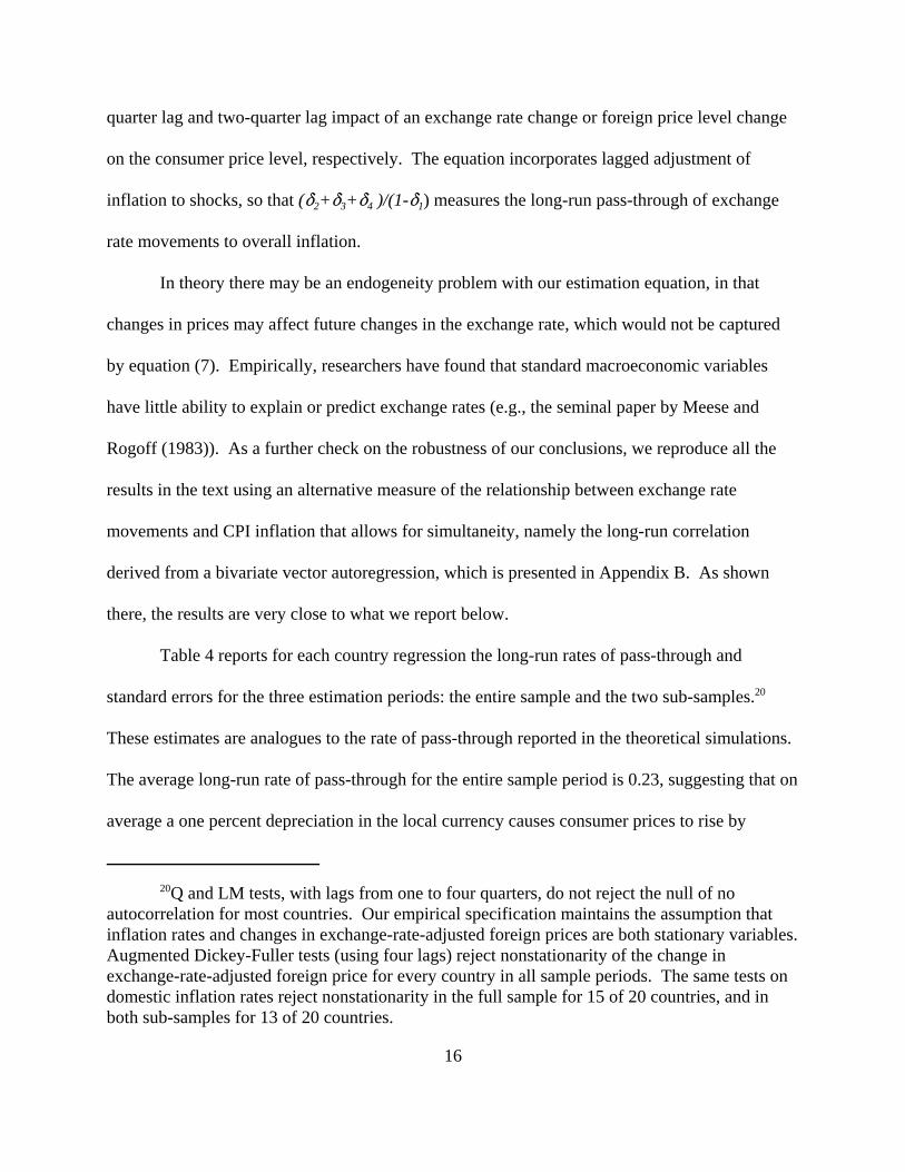
quarter lag and two-quarter lag impact of an exchange rate change or foreign price level change
on the consumer price level, respectively. The equation incorporates lagged adjustment of
inflation to shocks, so that (*2+*3+*4 )/(1-*1) measures the long-run pass-through of exchange
rate movements to overall inflation.
In theory there may be an endogeneity problem with our estimation equation, in that
changes in prices may affect future changes in the exchange rate, which would not be captured
by equation (7). Empirically, researchers have found that standard macroeconomic variables
have little ability to explain or predict exchange rates (e.g., the seminal paper by Meese and
Rogoff (1983)). As a further check on the robustness of our conclusions, we reproduce all the
results in the text using an alternative measure of the relationship between exchange rate
movements and CPI inflation that allows for simultaneity, namely the long-run correlation
derived from a bivariate vector autoregression, which is presented in Appendix B. As shown
there, the results are very close to what we report below.
Table 4 reports for each country regression the long-run rates of pass-through and
standard errors for the three estimation periods: the entire sample and the two sub-samples.20
These estimates are analogues to the rate of pass-through reported in the theoretical simulations.
The average long-run rate of pass-through for the entire sample period is 0.23, suggesting that on
average a one percent depreciation in the local currency causes consumer prices to rise by

17
approximately a quarter of a percent in the long run. Fourteen of the twenty countries’ rates of
pass-through are significantly different from zero. There is a wide dispersion of rates of pass-
through across countries, ranging from near zero in Sweden to 0.52 in Greece. The average
autoregressive coefficient, *1 , (not shown) is 0.7, implying a relatively quick pass-through. The
average R2 is 0.6.
The results for the two sub-samples show that there has been a decline in the rate of pass-
through in most countries. On average, the rate of pass-through fell from 0.16 in the first sub-
sample to 0.05 in the second sub-sample. In half of these countries the rate of pass-through is
significantly different between the two sample periods. For inflation targeters, the average rate
of pass-through was slightly higher than that for the other countries in the first sub-sample but it
fell below the average for the other countries in the second sub-sample, possibly indicating the
effects of stricter monetary responsiveness to inflation.
Before proceeding further, it is instructive to compare the magnitude of the decline in
pass-through measured here with that implied by Campa and Goldberg (2002), who estimate
pass-through to import prices over the samples 1975-89 and 1975-99. They find that long-run
pass-through declined in most OECD countries. However, it does not follow that the declines in
pass-through to CPIs are solely attributable to the declines in pass-through to import prices. The
average decline in the rate of import price pass-through from the short to the long sample in
Campa and Goldberg was no more than 0.04 (and less under alternative specifications). The
average change in pass-through to CPIs that we estimate is about three times as large. Moreover,
any direct effect on pass-through into CPIs of a change in pass-through at the import price level

18
would be further attenuated by the fact that even in the most open economies, many consumption
goods are produced locally and non-tradable services represent the majority of consumption.
III.B. Inflation Variability and Pass-Through in Industrial Countries
As the monetary authority becomes more vigilant and credible at fighting inflation, the
mean and standard deviation of inflation should fall. Thus, an indirect way of testing the
relationship between monetary policy and the rate of pass-through is to examine the link between
the rate of pass-through and the behavior of inflation.
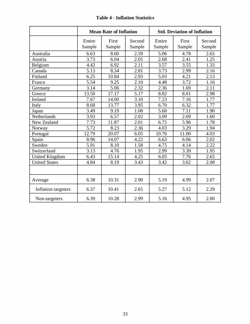
Table 3 reports summary statistics on inflation for the entire sample period and the two
sub-samples for each the twenty countries. The mean rate of inflation is lower in the second sub-
sample for every country and the standard deviation is lower for every country but Germany.
The magnitudes of these changes are not noticeably different on average between inflation
targeters and other countries. The following cross-country regressions of the rates of pass-
through (PT) on these inflation statistics for the full sample yield strongly significant
relationships.
(8.a) PT Mean p R= + =0 03 0 03 0 440 06 0 01
2. . ( ), .( . ) ( . )
*** ∆
(8.b)PT Std Dev p R= + =0 03 0 04 0 38
0 07 0 012. . ( ), .
( . ) ( . )
*** ∆
* * * indicates significant at the 99 percent confidence interval

19
Due to collinearity between the mean and standard deviation of inflation, we only include one of
the inflation statistics at a time. The results suggest that about one-third or more of cross-
country variation in pass-through can be attributed to the inflation environment. One potential
alternative explanation of cross-country variation in the rates of pass-through is the share of
imports in GDP; however, we find no statistical link between pass-through and the import share.
Moreover, including import shares in the above regressions does not significantly affect any of
the other coefficients.
Switching from the cross-country to the intertemporal information in the data, we
regressed changes in pass-through coefficients across sub-samples on changes in the inflation
statistics. Once again, there is a significant link, similar to that from the full-sample regressions.
Pass-through falls as the average rate of inflation falls and/or the volatility of inflation declines.
(9.a) ∆ ∆ ∆PT Mean p R= − + =0 01 0 01 0110 07 0 01
2. . * ( ), .( . ) ( . )
(9.b)
∆ ∆ ∆PT Std Dec p R= + =0 02 0 03 0 210 05 0 01
2. . ** ( ), .( . ) ( . )
*** (**) indicates significant at the 99 (95) percent confidence interval
A simple way to summarize these results is to plot the change in the rate of pass-through
against the change in the inflation statistics for each country. The top panel of Figure 2 plots the
change in the long-run rate of pass-through in a given country on the y axis against the change in

20
the mean rate of inflation on the x axis. The diagonal line represents the relationship estimated
in the above regression. Our theory implies that the rate of pass-through falls (rises) as the mean
rate of inflation declines (increases), so that country observations should lie in the shaded
regions of the graph. This relationship holds for 18 of the 20 countries in the sample. Turning to
the standard deviation of inflation, plotted in the bottom panel, the only outlier is Finland;
Germany’s rate of pass-through rose as did the standard deviation of German inflation.
These results are robust to the inclusion of more countries, including developing
countries. Choudhri, Faruqee, and Hakura (2002), for example, examine the correlation of pass-
through with the mean rate of inflation in a sample dominated by developing countries. As our
results and theoretical model suggest, however, lower variability of inflation may be the more
relevant factor behind lower rates of pass-through. But, given the strong empirical connection
between mean rates and standard deviations of inflation, it is not surprising that pass-through is
significantly correlated with both.
III.C. Monetary Policy in Industrial Countries
The evidence of the previous section is consistent with our hypothesis that monetary
policy has an important effect on pass-through. However, Table 2 showed that other economic
parameters can affect both inflation variability and pass-through. We believe that it is plausible
that changes in monetary policy are the primary factor behind the decline in inflation variability
over the past three decades, not least because the public record of central bank statements in
many countries indicates that there have been changes in objectives and/or procedures.
Nevertheless, this section develops a more direct test of the relationship between a monetary
21We include quarterly dummy variables to control for changes in indirect taxes that areincluded in consumer prices but are generally not targeted by central banks.
22Due to limited data on interest rates for Finland, New Zealand, Norway, Spain,Switzerland, and the United Kingdom, our sample for these countries begins in 1981:Q1,1974:Q4, 1972:Q3, 1978:Q1, 1973:Q1, and 1976:Q2, respectively.
21
authority’s emphasis on stabilizing inflation and the rate of pass-through. We start by estimating
a policy rule similar to that of Clarida, Gali and Gertler (1998) for each country. The estimation
is done on three sample periods: the entire sample and the split sample as before, allowing for a
change in the parameters across the two sub-samples.
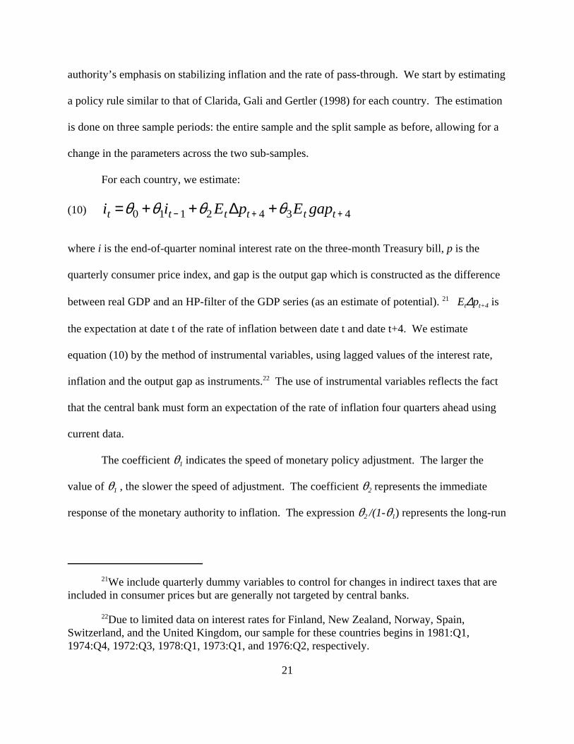
For each country, we estimate:
(10) i i E p E gapt t t t t t= + + +− + +θ θ θ θ0 1 1 2 4 3 4∆
where i is the end-of-quarter nominal interest rate on the three-month Treasury bill, p is the
quarterly consumer price index, and gap is the output gap which is constructed as the difference
between real GDP and an HP-filter of the GDP series (as an estimate of potential). 21 Et∆pt+4 is
the expectation at date t of the rate of inflation between date t and date t+4. We estimate
equation (10) by the method of instrumental variables, using lagged values of the interest rate,
inflation and the output gap as instruments.22 The use of instrumental variables reflects the fact
that the central bank must form an expectation of the rate of inflation four quarters ahead using
current data.
The coefficient 21 indicates the speed of monetary policy adjustment. The larger the
value of 21 , the slower the speed of adjustment. The coefficient 22 represents the immediate
response of the monetary authority to inflation. The expression 22 /(1-21) represents the long-run

23Because the regressors are themselves estimates (from Table 5) we weight theobservations in equations (11a) and (11b) by the standard errors of the regressions in which eachset of 2s was estimated.
22
response to inflation in the presence of slow adjustment (21 >0). Similarly, the long-run
response of the monetary authority to the output gap is 23 /(1-21).
Comparing our empirical equation to our theoretical model, the estimated long-run
response of monetary policy to inflation, 22 /(1-21), is comparable to : /(1-ρ5) in the theoretical
model. Similarly, the long-run output gap coefficient we estimate is the empirical analogue to
λ /(1-ρ5) . The lagged interest rate coefficient, 21 , is equivalent to ρ5 in our theoretical model.
For a monetary authority that moves to put more emphasis on low inflation, we expect to find an
increase in the estimated long-run inflation response and/or an increase in the speed of
adjustment (small coefficient value for 21). As discussed in Section II, the effect of the output
gap coefficient on inflation stabilization and pass-through is ambiguous.
Table 5 reports the long-run monetary policy coefficient estimates and the speed of
adjustment term for each country over the entire sample period. There is variation in the
coefficients across countries, particularly in the output gap coefficients. The large coefficient
standard errors indicate that most of these differences are not statistically significant. The
autoregressive coefficient averages 0.9, implying 30 percent of the long-run effect is transmitted
within one year.
Simulations from our theoretical model indicate that an increase in the inflation
coefficient or a faster response of monetary policy should decrease the rate of pass-through.
Attempts to link these monetary policy estimates with the corresponding estimated rates of pass-
through yield mixed results over the entire sample period (see equations (11.a) and (11.b)).23

23
These cross-country regressions do not show a significant link between the long-run inflation
coefficient and pass-through. However, they do find a statistically significant link between the
speed of monetary policy adjustment and pass-through.
(11.a) PT Sigma= −−
=0 24 0 031
0 310 09 0 10
2
1. ** . , .
( . ) ( . )
θθ
(11.b)
PT Sigma= +−
−−
+ =194 0 041
0 011
2 380 62 0 09
2
1 0 013
1 0 73 1. ** . . . *** ,( . ) ( . ) ( . ) ( . )
θθ
θθ
θ 0.10
***(**) indicates significant at the 99 (95) perent confidence interval)
If there have been important changes in monetary policy regimes during the sample, then
the above regression analysis may not miss much of the link between pass-through and monetary
policy. To address this problem, we estimate the monetary policy function separately in each
sub-sample and regress changes in the rate of pass-through on changes in the policy coefficients.
Table 6 reports the estimated policy rule results for the two sub-samples. There are
major differences between the sub-sample estimates. First, the average value of the long-run
inflation coefficient rises from 0.9 in the first sub-sample to 2.5 in the second sub-sample. The
increased coefficient value is apparent for both inflation targeters and other countries, although
the inflation targeters’ coefficients rise by a larger amount. Looking at the sub-samples, only the
24In the United States, core inflation is typically defined using the CPI excluding foodand energy.
25See Orphanides and Wilcox (1996).
24
United States has an estimate significantly different from zero in the first sample period, but in
the second sample period nearly half of the countries have significant inflation coefficients.
Second, the long-run gap coefficients increase in value from the first to second subsample.
However, the coefficients have large standard errors: notably the estimate for Portugal in the first
sample period and Australia in the second. We do not place much emphasis on these values.
Last, the speed of policy response falls (the lag coefficient rises) from the first to second sub-
samples.
In the second sub-sample most of the individual inflation coefficients are greater than the
minimum of unity for a unique stable solution to our theoretical model (and none of them are
significantly below unity). In the first sub-sample (as in the full sample) most of the inflation
coefficients are below unity. We believe that our coefficients are biased downward partly
because we use the volatile “headline” consumer price index instead of core domestic prices.24
We use the broad consumer price index because a consistent measure of core inflation is not
available for many countries. Another source of downward bias may be a change in the
monetary authority’s inflation target within the sample. Even within our sub-samples it is
possible that there were such shifts. For example, a monetary authority that pursued a strategy of
“opportunistic disinflation” would appear to have a weak reaction to changes in inflation when
inflation is falling, as it was in the United States during the 1990s.25 Finally, the low monetary
responses to inflation during the first sub-sample in many of these countries may be part of the

26The country weights used in this regression are the averages of the standard errors ofthe policy rule regressions in the two subsamples.
25
reason that they experienced great macroeconomic instability during the 1970s and 1980s. In
other words, choosing a policy parameter that is associated with multiple or explosive solutions
in the theoretical model may lead to instability in the real economy.
The implications of these changes in the policy rule coefficients across the subsamples on
the value of pass-through are mixed. On the one hand, a slower speed of adjustment in the
second sample period would tend to increase pass-through. But the higher long-run inflation
coefficient tends to reduce pass-through. From Table 6 we see the magnitude of the change in
the long-run inflation coefficient is much larger than that of the speed of adjustment term,
suggesting that the long-run inflation effect may dominate and push pass-through down.
This hypothesis is confirmed in the weighted regressions based on changes across sub-
samples.26
(12a) ∆ ∆PT Sigma= − − −−
=0 04 0 041
0110 03 0 02
2
1. . ** , .
( . ) ( . )
θθ
(12.b)
∆ ∆ ∆ ∆PT Sigma
indicataes significance at the level
= − −−
−−
+ =0 05 0 031
0 011
0 21 0110 03 0 01
2
1 0 013
1 0 16 1
95 90
. . * . * . , .( . ) ( . ) ( . ) ( . )
**(*) ( )% .
θθ
θθ
θ

26
These equations suggest that as a monetary authority increases its emphasis on fighting
inflation, which is depicted here as a positive value for 22 /(1-21), that the rate of pass-through
falls. This link is statistically significant in both regressions. The coefficient on the adjustment
speed (21) has the correct sign but is not significant. The output gap coefficient is significant but
small. Based on the link between pass-through and these policy-rule estimates, the effect of the
increased long-run emphasis on fighting inflation dominates the effect from a slower adjustment
process, resulting in pass-through declining over time.
Figure 3 plots the changes in the inflation coefficients against the changes in the
estimated rates of pass-through for each country. Our theoretical model implies that country
observations should lie in the northwest or southeast quadrants (highlighted in the figure); pass-
through falls (rises) as 22 /(1-21) rises (falls). Seventeen of the twenty countries lie in these
regions, with the Netherlands lying only slightly outside the region. The two outliers, Finland
and Portugal, have very large standard errors on the long-run inflation coefficients in the policy
rule (Table 6), suggesting that these observations should not be accorded much weight.
Our findings are consistent with a recent survey in the IMF’s World Economic Outlook
(May 2002) which looks at monetary policy in a low inflation era. The survey estimates
monetary policy rules for Canada, Germany, the United Kingdom, and the United States. It finds
that monetary policy in the 1980s and 1990s has been more responsive to changes in inflation
than in the 1970s. It then argues that this period of low and stable inflation has had a significant
effect on private sector behavior, such as a lengthening of wage contracts and a decline in
pricing power of firms. These changes in behavior can contribute to the declines in the rates of
pass-through we document.

27
To check on the robustness of our results, we also estimated the policy rules and pass-
through equations with alternative measures of potential output and with oil prices added to the
models. The results are similar: an increased emphasis on inflation by a monetary authority may
help to reduce the level of exchange rate pass-through.
IV. Conclusion
This paper documents a decline in measured exchange rate pass-through at the
macroeconomic level for many industrial countries since the 1980s. We develop a theoretical
model to explain how such a development could be the consequence of a shift in the monetary
authority’s responsiveness to inflation. When agents expect the monetary authority to act
strongly to stabilize the domestic inflation rate, they are less inclined to change prices in
response to a given exchange rate shock. We present evidence for a sample of 20 industrial
countries that supports this hypothesis indirectly and directly. First, we establish a robust and
significant connection between pass-through behavior and inflation variability. This is an
indirect test of the link between monetary policy and pass-through. Second, we uncover
evidence connecting increased emphasis in monetary policy on stabilizing inflation with lower
rates of pass-through.

28
References
Bank of Canada. 2000. Monetary Policy Report, November. Ottawa.
Brayton, F, JM Roberts, and JC Williams. 1999. What’s Happened to the Phillips Curve?Finance and Economics Discussion Series No. 1999-49. Board of Governors of the FederalReserve System.
Campa, JM, and LS Goldberg. 2002. Exchange Rate Pass-Through into Import Prices: A Macroor Micro Phenomenon? Staff Report No. 149. Federal Reserve Bank of New York.
Choudhri, E, H Faruqee, and D Hakura. 2002. Explaining the Exchange Rate Pass-Through inDifferent Prices. Working Paper WP/02/224. International Monetary Fund.
Christiano, L, M Eichenbaum, and C Evans. 2001. Nominal Rigidities and the Dynamic Effectsof a Shock to Monetary Policy. National Bureau of Economic Research Working Paper No.8403.
Clarida, R, J Gali, and M Gertler. 1998. Monetary Policy Rules in Practice: Some InternationalEvidence. European Economic Review 42: 1033-67.
Cunningham, A, and A Haldane. 1999. The Monetary Transmission Mechanism in the UnitedKingdom: Pass-Through and Policy Rules. manuscript. Bank of England.
Devereux, M, C Engel, and P Storgaard. 2003. Endogenous Exchange Rate Pass-Through WhenNominal Prices Are Set in Advance. National Bureau of Economic Research Working Paper No.9543.
Fair, RC. 2001. Actual Federal Reserve Policy Behavior and Interest Rate Rules. FederalReserve Bank of New York Economic Policy Review 7: 61-71.
Freedman, C. 1994. The Use of Indicators and of the Monetary Conditions Index in Canada. inBaliño and Cottarelli (eds.) Frameworks for Monetary Stability: Policy Issues and CountryExperiences. International Monetary Fund.
Freeman, RT, and JL Willis. 1995. Targeting Inflation in the 1990s: Recent Challenges.International Finance Discussion Papers No. 525. Board of Governors of the Federal ReserveSystem.
Froot, K, and R Thaler. 1990. Anomalies: Foreign Exchange. Journal of Economic Perspectives4: 179-92.
Fuhrer, J, and G Moore. 1995. Inflation Persistence. Quarterly Journal of Economics 110: 127-59.

29
Goldberg, PK, and MM Knetter. 1997. Goods Prices and Exchange Rates: What Have WeLearned? Journal of Economic Literature 35: 1243-72.
Goldfajn, I, and SR Werlang. 2000. The Pass-Through from Depreciation to Inflation: A PanelStudy. Banco Central do Brasil Working Paper Series No. 5.
Leahy, M. 1998. New Sumary Measures of the Foreign Exchange Value of the Dollar. FederalReserve Bulletin, 84: 811-818.
Parsley, D, and H Popper. 1998. Exchange Rates, Domestic Prices, and Central Bank Actions:Recent U.S. Experience. Southern Economic Journal 64: 957-72.
Hooper, P, K Johnson, and J Marquez. 2000. Trade Elasticities for the G-7 Countries. PrincetonStudies in International Economics No. 87. Princeton University.
International Monetary Fund. 1996. World Economic Outlook, May.
______. 2002. World Economic Outlook, May.
Kamin, SB. 1998. A Multi-Country Comparison of the Linkages between Inflation andExchange Rate Competitiveness. International Finance Discussion Papers No. 603. Board ofGovernors of the Federal Reserve System.
Laflèche, T. 1996. The Impact of Exchange Rate Movements on Consumer Prices. Bank ofCanada Review Winter 1996-1997: 21-32.
Lubik, T, and F Schorfheide. 2004. Testing for Indeterminacy: An Application to U.S. MonetaryPolicy. American Economic Review 94: 190-217.
McCarthy, J. 2000. Pass-Through of Exchange Rates and Import Prices to Domestic Inflation inSome Industrialized Economies. Federal Reserve Bank of New York Staff Report 111.
Meese, R and K Rogoff. 1983. Empirical Exchange Rate Models of the Seventies: Do They FitOut of Sample? Journal of International Economics 14: 3-24.
Nelson, E. 2000. UK Monetary Policy 1972-1997: A Guide Using Taylor Rules. manuscriptISSN 1368-5562. Bank of England.
Norambuena, CN. 2003. The Pass-Through from Depreciation to Inflation: Chile 1986-2001.Estudios de Economia 30: 133-55.
Olivei, GP. 2002. Exchange Rates and the Prices of Manufacturing Products Imported into theUnited States. New England Economic Review First Quarter: 3-18. Federal Reserve Bank ofBoston.

30
Orphanides, A, and DW Wilcox. 1996. The Opportunistic Approach to Disinflation. Finance andEconomics Discussion Series No. 1996-24. Board of Governors of the Federal Reserve System.
Reifschneider, D, R Tetlow, and J Williams. 1999. Aggregate Disturbances, Monetary Policy,and the Macroeconomy: The FRB/US Perspective. Federal Reserve Bulletin 85: 1-19.
Taylor, JB. 1993. Discretion versus Policy Rules in Practice. Carnegie-Rochester Conference onPublic Policy 39: 195-214.
______. 2000. Low Inflation, Pass-Through, and the Pricing Power of Firms. EuropeanEconomic Review 44: 1389-1408.
Woodford, M. 2003. Interest and Prices: Foundations of a Theory of Monetary Policy. PrincetonUniversity Press: Princeton, NJ.

31
Table 1 - Model and Data Sample Moments
Autoregressive Coefficient Standard Deviation
y )p e+p*-p i )y )p )(e+p*-p) )i
Model* .79 .32 .91 .90 .95 .53 3.60 .84
Data** .76 .38 .91 .91 .84 .53 3.54 .82
*Average over 10,000 Monte Carlo simulations using Base case parameters.**Average over 20 industrial countries in the second sub-sample described in Section III of this paper.
Table 2 - Theoretical Model (Equations 1-6)
Pass-Through Coefficient* Standard Deviation of Inflation
Base** :=1.5 8=1.0 D5=0 Base** :=1.5 8=1.0 D5=0
Base .11 .18 .11 .09 .15 .19 .16 .15
"=.3 .25 .50 .24 .21 .17 .24 .17 .17
$=.5 .15 .30 .15 .13 .16 .22 .16 .16
(=.02 .15 .31 .15 .10 .16 .22 .16 .15
N=.2 .25 .30 .25 .24 .27 .29 .27 .27
Fu=0 .10 .17 .11 .09 .15 .19 .16 .15
Fv=0 .90 .96 .93 .85 .13 .15 .14 .13
Fx=0 .07 .13 .06 .06 .11 .15 .11 .11
Fz=0 .14 .24 .13 .10 .13 .17 .13 .12
*Long-run coefficient from regression of inflation rate on exchange rate changes with intercept and lags.**The Base case is equations (1) through (6) with "=.1, $=1.0, (=.005, N=.05, :=2.0, 8=.5, B=0,D1=D2=D3=D5=0.5, D4=0.95, Fu=0.2, Fv=0.1, Fw=0.2, Fx=.05, and Fz=.08.

32
Table 3 - Long-run Rates of Pass-through
Entire Sample First Sample Second SampleAustralia 0.14
(0.07)0.09
(0.08)0.01
(0.04)Austria 0.11
(0.07)0.06
(0.10)0.04
(0.02)Belgium 0.20
(0.08)0.21
(0.09)0.02
(0.02)Canada 0.37
(0.11)0.30
(0.14)0.04
(0.06)Finland 0.01
(0.14)-0.11(0.21)
0.00(0.03)
France 0.23(0.12)
0.17(0.07)
0.01(0.03)
Germany 0.11(0.04)
-0.13(0.11)
0.12(0.03)
Greece 0.52(0.11)
0.28(0.12)
0.27(0.21)
Ireland 0.29(0.09)
0.18(0.11)
0.06(0.04)
Italy 0.37(0.12)
0.33(0.09)
0.08(0.06)
Japan 0.21(0.09)
0.26(0.12)
0.02(0.02)
Netherlands 0.16(0.07)
0.08(0.11)
0.06(0.03)
New Zealand 0.42(0.10)
0.29(0.09)
0.01(0.05)
Norway 0.28(0.15)
0.11(0.17)
-0.05(0.06)
Portugal 0.43(0.08)
0.37(0.08)
0.17(0.16)
Spain 0.18(0.09)
0.14(0.07)
0.03(0.03)
Sweden 0.02(0.07)
0.05(0.05)
0.02(0.02)
Switzerland 0.15(0.09)
0.18(0.14)
0.07(0.08)
United Kingdom 0.15(0.05)
0.18(0.08)
0.08(0.05)
United States 0.27(0.12)
0.19(0.36)
0.03(0.06)
Average 0.23 0.16 0.05 Inflation targeters 0.22 0.18 0.03 Non-targeters 0.23 0.15 0.06
Standard errors in parenthesis.
33
Table 4 - Inflation Statistics
Mean Rate of Inflation Std. Deviation of Inflation
EntireSample
FirstSample
SecondSample
EntireSample
FirstSample
SecondSample
Australia 6.63 8.60 2.59 5.06 4.78 2.65Austria 3.73 6.04 2.05 2.68 2.41 1.25Belgium 4.42 6.92 2.11 3.57 3.55 1.33Canada 5.13 8.34 2.81 3.73 2.99 2.16Finland 6.25 10.84 2.93 5.03 4.21 2.13France 5.54 9.25 2.10 4.48 3.72 1.16Germany 3.14 5.06 2.32 2.36 1.69 2.11Greece 13.50 17.17 5.17 8.82 8.01 2.98Ireland 7.67 14.00 3.10 7.23 7.16 1.77Italy 8.68 13.77 3.95 6.70 6.32 1.77Japan 3.49 9.19 1.08 5.60 7.11 1.90Netherlands 3.93 6.57 2.02 3.09 2.69 1.60New Zealand 7.73 11.87 2.01 6.75 5.96 1.78Norway 5.72 8.23 2.36 4.03 3.29 1.94Portugal 12.79 20.07 6.05 10.76 11.00 4.03Spain 8.96 14.07 4.22 6.63 6.06 2.02Sweden 5.91 8.10 1.58 4.75 4.14 2.22Switzerland 3.13 4.76 1.95 2.99 3.39 1.95United Kingdom 6.43 15.14 4.25 6.05 7.76 2.65United States 4.84 8.19 3.43 3.42 3.62 2.08
Average 6.38 10.31 2.90 5.19 4.99 2.07
Inflation targeters 6.37 10.41 2.65 5.27 5.12 2.29
Non-targeters 6.39 10.28 2.99 5.16 4.95 2.00

34
Table 5 - Policy Rule, Full sample
22 /(1-21) 23 /(1-21) 21
Australia 1.02(0.41)
2.90(3.29)
0.89(0.04)
Austria 0.79(0.38)
-0.21(1.11)
0.89(0.04)
Belgium 1.06(0.62)
3.69(5.64)
0.93(0.05)
Canada 2.57(3.21)
18.95(31.08)
0.96(0.05)
Finland 1.38(0.83)
1.89(2.06)
0.91(0.06)
France 1.24(1.05)
13.70(19.95)
0.96(0.05)
Germany 1.38(0.37)
1.62(0.93)
0.87(0.05)
Greece 1.41(0.65)
-0.41(1.70)
0.97(0.02)
Ireland 0.59(0.35)
2.91(2.77)
0.90(0.05)
Italy 1.20(0.54)
3.17(3.78)
0.92(0.04)
Japan 1.05 (0.23)
0.50(1.56)
0.88(0.03)
Netherlands 0.45(0.44)
4.46(3.17)
0.85(0.07)
New Zealand 0.55(0.30)
2.90(2.22)
0.87(0.05)
Norway 0.60(0.33)
-0.96(1.04)
0.86(0.05)
Portugal 1.04(0.56)
-2.28(2.77)
0.97(0.02)
Spain 0.89(0.26)
1.35(2.06)
0.82(0.06)
Sweden 0.66(0.30)
-1.21(1.02)
0.86(0.05)
Switzerland 0.61(0.43)
2.45(1.57)
0.87(0.06)
United Kingdom 1.03(0.61)
4.42(6.19)
0.94(0.06)
United States 0.93(0.37)
1.13(1.39)
0.86(0.06)
Average 1.02 3.05 0.90 Inflation targeters 1.17 5.59 0.90 Non-targeters 0.97 2.20 0.90
Standard errors in parenthesis.

35
Table 6 - Policy Rule, Sub-samples
First Sample Second Sample
22 /(1-21) 23 /(1-21) 21 22 /(1-21) 23 /(1-21) 21
Australia 0.72(0.57)
2.22(2.89)
0.86(0.06)
4.84(14.52)
-0.01(6.66)
0.97(0.09)
Austria 0.24(0.70)
-1.29(0.96)
0.84(0.08)
1.74(0.63)
0.58(0.82)
0.82(0.07)
Belgium 0.25(0.40)
-0.69(1.30)
0.83(0.08)
3.19(2.02)
1.61(2.79)
0.92(0.06)
Canada 0.73(0.82)
0.46(1.95)
0.86(0.08)
2.13(0.95)
4.11(3.84)
0.91(0.06)
Finland -0.29(0.21)
-1.25(0.61)
0.12(0.22)
0.88(4.88)
3.91(9.66)
0.96(0.08)
France 0.60(0.53)
0.34(3.04)
0.87(0.08)
3.04(1.64)
2.77(3.95)
0.90(0.07)
Germany 3.21(1.67)
2.09(3.03)
0.84(0.16)
1.85(0.33)
-0.09(0.31)
0.78(0.09)
Greece -0.06(0.70)
-1.14(2.20)
0.97(0.02)
0.58(0.72)
-7.68(4.01)
0.89(0.04)
Ireland -0.27(0.35)
0.61(1.34)
0.83(0.09)
1.29(3.63)
3.55(3.86)
0.91(0.07)
Italy 0.75(0.72)
-1.15(1.31)
0.85(0.09)
2.67(0.51)
-0.20(2.65)
0.76(0.16)
Japan 2.16(4.52)
5.25(14.92)
0.92(0.15)
2.16(0.53)
1.06(1.07)
0.91(0.04)
Netherlands 0.27(0.41)
0.70(1.02)
0.66(0.13)
-3.08(4.63)
9.15(11.54)
0.98(0.03)
New Zealand -0.37(0.49)
-0.04(1.36)
0.76(0.08)
8.21(8.70)
-1.94(2.11)
0.93(0.06)
Norway 0.04(0.42)
0.16(0.50)
0.79(0.08)
10.00(8.22)
1.64(2.97)
0.85(0.09)
Portugal 7.01(17.17)
-13.34(31.69)
0.99(0.03)
1.67(0.74)
4.08(5.17)
0.94(0.05)
Spain 0.67(0.34)
-2.41(2.15)
0.40(0.16)
3.81(0.67)
-1.34(1.30)
0.77(0.09)
Sweden 0.09(0.59)
-0.93(0.83)
0.79(0.08)
0.65(1.15)
0.88(1.18)
0.89(0.05)
Switzerland 0.52(0.56)
1.16(1.61)
0.79(0.14)
0.54(1.97)
2.71(5.78)
0.95(0.08)
United Kingdom 0.87(0.61)
-0.53(0.93)
0.63(0.31)
1.76(0.33)
1.37(0.95)
0.83(0.06)
United States 0.90(0.32)
-0.11(0.42)
0.52(0.18)
2.24(0.65)
0.73(0.76)
0.84(0.06)
Average 0.90 -0.49 0.76 2.51 1.34 0.89 Inflation targeters 0.41 0.24 0.78 3.52 0.88 0.91 Non-targeters 1.07 -0.74 0.75 2.17 1.50 0.88
Standard errors in parenthesis.

36
Appendix A
All data are available from authors upon request.
∆p = quarterly domestic inflationInflation is measured as the change in the consumer price index that the country’s central banktargets (for the United Kingdom we use the RPIX). The original source of all the indexes are thenational statistic office, seasonally adjusted at the source or by authors.
∆(e+p*) = exchange-rate adjusted foreign consumer prices, quarterly rateThis series is ∆(p/RER), where RER is the real exchange rate defined as foreign/domesticcurrency, and the price measures are the same as used in the inflation series. The real exchangerate is a seasonally adjusted trade-weighted measure that is constructed by the authors (exceptGreece, New Zealand and Norway which are OECD data). For a detailed discussion of theconstruction and trade weights see Leahy (1998).
y = output gap in percentage points, quarterlyThe gap is (GDP-GDP*)/GDP*. GDP data are from International Financial Statistics, exceptBelgium, Greece, Ireland, Netherlands, New Zealand, and Portugal that come from Haver. GDP*is potential GDP, which we construct from a standard H-P filtering of the GDP series.
i= nominal 3 month interest rate, annualizedThe measure and source varies by country as noted in the table.
country series source
Australia 3-month bank-accepted bills
Haver
Austria* 3-month moneymarket rate(3-month moneymarket rate)
Haver(IFS)
Belgium 3-month Treasury billrate
Haver
Canada 3-month Treasury billrate
IFS
Finland* 3-month moneymarket rate
Haver
France* Treasury bill rate IFS
Germany 3-month interbank rate(FIBOR)
Haver
Greece Commercial bankdeposit rate
IFS
Ireland 3-month interbank rate(3-month moneymarket rate)
Haver(Haver)
Italy 3-month interbank rate Haver
Japan 3-month Gensaki rate Haver
country series source
Nether-lands*
3-month interbank rate Haver
NewZealand
90-day bank bill rate(90-day bank bill rate)
Haver(OECD)
Norway 3-month moneymarket rate (NIBOR)(Call money rate)
BIS(IFS)
Portugal 3-month interbank rate(3-month moneymarket rate)
Haver(Haver)
Spain 3-month interbank rate Haver
Sweden 3-month Treasury billrate(3-month Treasurydiscount note rate)
Bloomberg(IFS)
Switzer-land
3-month Treasury billrate(Call money rate)
IFS(OECD)
U.K. 3-month Treasury billaverage discount rate
Haver
U.S. 3-month Treasury billrate
IFS
*3-month EURIBOR used for 1999:1 - 2003:4 (Haver).Series and sources in parentheses used to estimate missing periods in primary data source.

37
Second Sample Period
country period
Australia 1993:2-2003:4
Austria 1985:1-2003:4
Belgium 1987:1-2003:4
Canada 1985:1-2003:4
Finland 1985:1-2003:4
France 1987:1-2003:4
Germany 1981:1-2003:4
Greece 1994:1-2003:3
Ireland 1985:1-2003:4
Italy 1987:1-2003:4
Japan 1981:1-2003:4
Netherlands 1985:1-2003:4
New Zealand 1990:2-2003:3
Norway 1990:1-2003:3
Portugal 1987:1-2003:4
Spain 1987:1-2003:4
Sweden 1993:1-2003:4
Switzerland 1985:1-2003:4
U.K. 1981:1-2003:4
U.S. 1981:1-2003:4

38
Individual Country Tax Dummies* (Dummies for changes in tax policies)
country tax policy change
Australia 2000:3
Austria 1999:1 (policy only)
Canada* 1991:1, 1994:1, 1994:2
Finland 1999:1 (policy only)
Greece 1994:2 (policy only), 1996:1
Japan 1989:2, 1997:2
Netherlands 1999:1 (policy only)
Sweden 1991:1, 1992:1, 1993:1
United Kingdom 1979:3* All dummies set equal to one in the appropriate quarter, except Canada’s 1994 VAT change that was phased inover two quarters so we set the dummy as 1994:1 = 2/3, 1994:2 = 1/3.

39
∆ ∆ ∆p p e pt i t i
jj t j t j t
i= + ∑ + + +
= −=
− −∑γ γ γ ε0
0
3
1
3
( * )
∆ ∆ ∆( * ) ( * ) *e p e p pt t i t i t i j t ij ti j
+ = ∑ + + ∑ ++− − −= =
β β β µ0 1
3
0
3
Appendix BEstimates of the Long-run Correlation
In this appendix we provide an alternative methodology for estimating the relationship betweenmovements in consumer prices and movements in exchange rates. Allowing for the possibilitythat there may be endogenity between inflation and exchange rate movements, here we estimatea bivariate vector autoregression between these two variables for each country and each sampleperiod, and consider the long-run correlations from this analysis. The equation we estimate is:
From these equations we back out the long-run covariance and variance of the two variables andcalculate the long-run correlation. As shown below, these long-run correlation estimates arecorrelated with the long-run pass-through estimates we use in the main text and the conclusionswe draw from the long-run pass-through estimates are reproduced using the long-run correlationestimates, suggesting our results are robust to the issue of simultaneity between movements inconsumer prices and movements in exchange rates.
Table B1 lists the estimated long-run correlations along with the long-run pass-throughestimates. The average long-run correlation coefficient is 0.75 while the average long-run pass-through estimate is 0.23. These two measures do not need to be similar in value. The long-runcorrelation estimate signals the strength of association between exchange rate movements andprices over the long run, and is independent of particular units of measurement; the long-runpass-through coefficient depends on the relative magnitudes of changes in the variables, as itindicates the quantity of the change in the exchange rate that feeds into the price level in the longrun. The correlation between the two measures over the full sample is 0.68. Looking at the sub-samples, the correlation between the two measures is higher in the first sample period than thesecond.
Table B1 - Estimates of long-run correlations and long-run pass-through (full sample)
Country Estimate of Long-run
Correlation Pass-through
Australia 0.751 0.144
Austria 0.649 0.108
Belgium 0.784 0.202
Canada 0.763 0.371
Finland 0.619 0.008

40
France 0.911 0.229
Germany 0.674 0.110
Greece 0.943 0.520
Ireland 0.892 0.290
Italy 0.869 0.366
Japan 0.702 0.206
Netherlands 0.767 0.156
New Zealand 0.897 0.421
Norway 0.865 0.276
Portugal 0.900 0.435
Spain 0.863 0.185
Sweden 0.539 0.021
Switzerland 0.349 0.151
U.K. 0.417 0.152
U.S. 0.759 0.268
Correlation 0.68
Using the long-run correlation estimates in place of the long-run pass-through estimates, wererun the weighted regressions in the text. We find that the long-run correlation between the rateof inflation and changes in exchange rates reacts almost identically to the inflation statistics asthe long-run pass-through estimates reported in the text. For example, looking at the cross-section relationship between the long-run correlation estimate and inflation statistics over theentire sample, we find coefficient estimates similar in value and significance. That is, rerunningequations 8a and 8b with the dependent variable replaced by the long-run correlation estimate,we find:
C .36 + 0.04 Mean( p), R 0.20***
(0.02)
** 2orr = =00 12( . )
∆
C 0.33 0.06 Std Dev( p), R 0.22**
(0.13)
** 2
* * * (**) indicates signficant at the 99 (95) percent confidence interval
orr = + =( . )0 02
∆

41
C .76 - 0.021-
, Sigma = 0.39***
(0.13)
2
1orr = 0
0 12( . )
θθ
C -0.76 + 0.08 0.01 +1.560 , igma = 0.14(0.12) (0.01) (1.06)
orr S=−
−−( . )0 90
2
1
3
111 1
θθ
θθ θ
Next equations 9a and 9b, which focus on changes across sub-samples, find similar results.
∆ ∆ ∆Corr 0.15 + 0.08 Mean( p), R 0.30(0.02)
*** 2= =( . )0 17
∆ ∆ ∆Corr = + = - 0.12 0.07 Std Dev( p), R 0.04(0.14)
2
* * * indicates signficant at the 99 percent confidence interval( . )0 03
There is a more significant link with changes in inflation than found in the text using the changein long-run pass-through, while the relationship between the long-run correlation and thestandard deviation of inflation is weaker than what we found in the long-run pass-throughregression. These results are suggestive that graphs similar to what is shown in Figure 2 wouldconvey the same point, as they do.
Linking long-run correlations to monetary policy, similar in manner to equations 11 and 12 inthe text, we find the data support our hypothesized link between increased emphasis on fightinginflation and reductions in the correlation between the rate of inflation and changes in theexchange rate. Actually, the weighted regressions that estimate the impact of a change in thelong-run Policy rule inflation coefficient on the change in the correlation are more significantthan what is found in the text.
∆ ∆Corr Sigma=−
= .08 - 0.18** 0.32(0.05)
010 10
2
1( . )* ,
θθ
∆ ∆ ∆ ∆C -0.02 - 0 .06 0.03 - 0.04 , Sigma = 0.28
**(***)(0.02) (0.02) (0.42)
indicates significant at the 95 (99)% level.
orr =−
−−( . )
**0 09
2
1
3
111 1
θθ
θθ θ
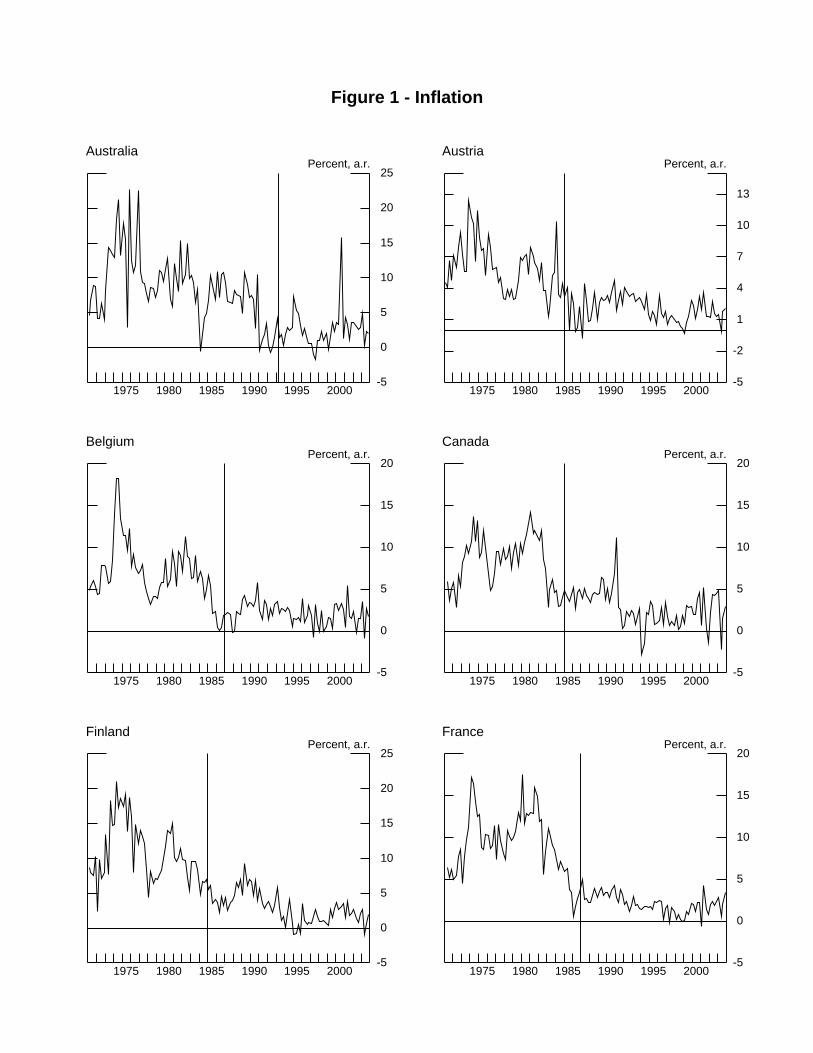
Figure 1 - Inflation
1975 1980 1985 1990 1995 2000-5
0
5
10
15
20
25
AustraliaPercent, a.r.
1975 1980 1985 1990 1995 2000-5
-2
1
4
7
10
13
AustriaPercent, a.r.
1975 1980 1985 1990 1995 2000-5
0
5
10
15
20
BelgiumPercent, a.r.
1975 1980 1985 1990 1995 2000-5
0
5
10
15
20
CanadaPercent, a.r.
1975 1980 1985 1990 1995 2000-5
0
5
10
15
20
25
FinlandPercent, a.r.
1975 1980 1985 1990 1995 2000-5
0
5
10
15
20
FrancePercent, a.r.

1975 1980 1985 1990 1995 2000-2
0
2
4
6
8
10
GermanyPercent, a.r.
1975 1980 1985 1990 1995 20000
10
20
30
40
50
GreecePercent, a.r.
1975 1980 1985 1990 1995 2000-10
0
10
20
30
40
IrelandPercent, a.r.
1975 1980 1985 1990 1995 20000
10
20
30
40
ItalyPercent, a.r.
1975 1980 1985 1990 1995 2000-10
0
10
20
30
40
50
JapanPercent, a.r.
1975 1980 1985 1990 1995 2000-5
0
5
10
15
NetherlandsPercent, a.r.

1975 1980 1985 1990 1995 2000-10
0
10
20
30
40
50
New ZealandPercent, a.r.
1975 1980 1985 1990 1995 2000-5
0
5
10
15
20
NorwayPercent, a.r.
1975 1980 1985 1990 1995 2000-20
-10
0
10
20
30
40
50
60
PortugalPercent, a.r.
1975 1980 1985 1990 1995 20000
10
20
30
40
SpainPercent, a.r.
1975 1980 1985 1990 1995 2000-5
0
5
10
15
20
25
SwedenPercent, a.r.
1975 1980 1985 1990 1995 2000-5
0
5
10
15
20
SwitzerlandPercent, a.r.

1975 1980 1985 1990 1995 20000
10
20
30
40
United KingdomPercent, a.r.
1975 1980 1985 1990 1995 2000-5
0
5
10
15
20
United StatesPercent, a.r.
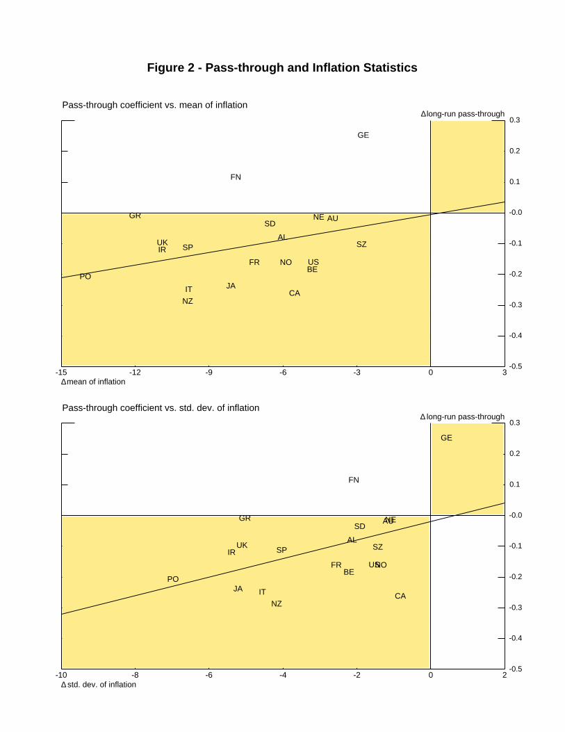
Figure 2 - Pass-through and Inflation Statistics
-10 -8 -6 -4 -2 0 2-0.5
-0.4
-0.3
-0.2
-0.1
-0.0
0.1
0.2
0.3
Pass-through coefficient vs. std. dev. of inflationlong-run pass-through
AL
AU
BE
CA
FN
FR
GE
GR
IR
ITJA
NE
NZ
NO
PO
SP
SD
SZUK
US
∆
∆ std. dev. of inflation
-15 -12 -9 -6 -3 0 3-0.5
-0.4
-0.3
-0.2
-0.1
-0.0
0.1
0.2
0.3
Pass-through coefficient vs. mean of inflationlong-run pass-through
AL
AU
BE
CA
FN
FR
GE
GR
IR
IT JA
NE
NZ
NO
PO
SP
SD
SZUK
US
∆
∆ mean of inflation

Figure 3 - Pass-through and Monetary Policy
-6 -4 -2 0 2 4 6 8 10-0.4
-0.3
-0.2
-0.1
-0.0
0.1
0.2
0.3
Pass-through coefficient vs. long-run inflation coefficientlong-run pass-through
AL
AU
BE
CA
FN
FR
GE
GR
IR
ITJA
NE
NZ
NO
PO
SP
SD
SZ UK
US
∆
∆ θ / 1−θ2 1