WP/13/209

Monetary and Macroprudential Policy in an Estimated DSGE Model of the Euro

Area

Dominic Quint and Pau Rabanal

© 2013 International Monetary Fund WP/13/209

IMF Working Paper

Institute for Capacity Development

Monetary and Macroprudential Policy in an Estimated DSGE Model of the Euro Area1

Prepared by Dominic Quint and Pau Rabanal

Authorized for distribution by Jorge Roldós

October 2013

Abstract

This Working Paper should not be reported as representing the views of the IMF, its Executive Board, or its management. The views expressed in this Working Paper are those of the author(s) and do not necessarily represent those of the IMF or IMF policy. Working Papers describe research in progress by the author(s) and are published to elicit comments and to further debate.

In this paper, we study the optimal mix of monetary and macroprudential policies in an estimated two-country model of the euro area. The model includes real, nominal and financial frictions, and hence both monetary and macroprudential policy can play a role. We find that the introduction of a macroprudential rule would help in reducing macroeconomic volatility, improve welfare, and partially substitute for the lack of national monetary policies. Macroprudential policy would always increase the welfare of savers, but their effects on borrowers depend on the shock that hits the economy. In particular, macroprudential policy may entail welfare costs for borrowers under technology shocks, by increasing the countercyclical behavior of lending spreads.

JEL Classification Numbers: C51; E44, E52. Keywords: Monetary Policy, EMU, Basel III, Financial Frictions. Author’s E-Mail Address: dominic.quint@fu-berlin.de; prabanal@imf.org

1 We thank Helge Berger, Larry Christiano, Chris Erceg, Ivo Krznar, Vivien Lewis, Jesper Lindé, Olivier Loisel, Stephen Murchinson, Jorge Roldós, Thierry Tressel and participants at various conferences and seminars for useful comments and discussions. Dominic Quint is a Ph.D. candidate at the Free University of Berlin. Pau Rabanal is a senior economist at the Institute for Capacity Development of the IMF.

2

Contents Page

I. Introduction .......................................................................................................................4

II. The Model .........................................................................................................................7A. Credit Markets ............................................................................................................8

A.1 Domestic intermediaries ......................................................................................8 A.2 International intermediaries ...............................................................................11

B. Households ................................................................................................................12 B.1 Savers .................................................................................................................12 B.2 Borrowers ...........................................................................................................13

C. Firms, Technology and Nominal Rigidities ..............................................................14 C.1 Final goods producers ........................................................................................15 C.2 Intermediate goods producers ............................................................................16

D. Closing the Model .....................................................................................................16 D.1 Market clearing conditions.................................................................................16 D.2 Monetary policy and interest rates .....................................................................18

III. Parameter Estimates ........................................................................................................18A. Data ...........................................................................................................................19 B. Calibrated Parameters ...............................................................................................19 C. Prior and Posterior Distributions ..............................................................................20 D. Model Fit and Variance Decomposition ...................................................................23 E. Model Comparison: A Brief Discussion ...................................................................25

IV. Policy Experiments .........................................................................................................26A. Optimal Monetary Policy ..........................................................................................28

A.1 Estimated Taylor rule .........................................................................................28 A.2 Extending the Taylor rule with financial variables ............................................28

B. Macroprudential Regulation .....................................................................................29 B.1 Regulation at the EMU-level .............................................................................30 B.2 Regulation at the national level ..........................................................................34

V. Conclusions .....................................................................................................................35

References ................................................................................................................................36

Appendix ..................................................................................................................................40

Text Table 1. Calibrated Parameters .....................................................................................................202. Priors and Posteriors .......................................................................................................223. Posterior Second Moments in the Data and in the Model ..............................................244. Correlation Matrix ..........................................................................................................255. Optimal Taylor Rule Coefficients ...................................................................................286. Optimal Monetary and Macroprudential Policy at the EMU Level ...............................317. Optimal Monetary and Macroprudential Policy, Conditional on Shocks .......................34

3

Figures 1a. Impulse Response to a Housing Demand Shock in the Periphery ..................................53 1b. Impulse Response to a Housing Demand Shock in the Periphery ..................................54 2a. Impulse Response to a Risk Shock in the Periphery .......................................................55 2b. Impulse Response to a Risk Shock in the Periphery .......................................................56 3a. Impulse Response to a Permanent Technology Shock in the EMU ...............................57 3b. Impulse Response to a Permanent Technology Shock in the EMU ...............................58 4. Best Responses when Macro-Prudential Policies Maximize Domestic Welfare ............59

4

I. Introduction

The recent �nancial crisis, that started in the summer of 2007, lead to the worstrecession since World War II. Before the crisis, a combination of loose monetary andregulatory policies encouraged excessive credit growth and a housing boom in manycountries. This turned out to be a problem when the world economy slowed down:as Claessens, Kose and Terrones (2008), Crowe et al. (2013) and IMF (2012) show,the combination of credit and housing boom episodes ampli�es the business cycleand in particular, the bust side of the cycle (measured as the amplitude andduration of recessions). Excessive leverage has complicated the recovery and thereturn to pre-crisis growth rates in several advanced countries, in particular in thegroup of peripheral European countries now known as GIIPS (Greece, Ireland, Italy,Portugal and Spain). Developments in those countries since the launch of theEuropean Economic and Monetary Union (EMU) in 1999 shared manycharacteristics with the run-up to other crises. Real exchange rate appreciation(which in the EMU took the form of persistent in�ation di¤erentials), large capitalin�ows mirrored by large current account de�cits, and above-potential GDP growthrates fuelled by cheap credit as well as asset price bubbles are the traditionalsymptoms of ensuing �nancial, banking and balance of payments crises in emergingand developed economies alike.1 In addition to all these overheating symptoms, theGIIPS countries faced prolonged negative real interest rates, which magni�ed theboom side of the business cycle. When the crisis hit, all problems came at once: asudden stop of capital �ows, concerns about debt sustainability, low or negative realGDP growth, and increased credit spreads that helped to amplify the bust side ofthe business cycle.

There is an increasing consensus that the best way to avoid a large recession in thefuture is precisely to reduce the volatility of credit cycles and their e¤ects on thebroader macroeconomy.2 However, the search for the appropriate toolkit to dealwith �nancial and housing cycles is still in its infancy. There is high uncertainty onwhich measures can be more e¤ective at delivering results. Conventional monetarypolicy is too blunt of an instrument to address imbalances within the �nancial sectoror overheating in one sector of the economy (such as housing). There is a need tofurther strengthen other instruments of economic policy in dealing withsector-speci�c �uctuations.3 In particular, a key question to be addressed is the roleof macroprudential regulation. Should it be used as a countercyclical policy tool,leaning against the wind of large credit, asset and house price �uctuations, or should

1See Kaminsky and Reinhart (1999) and IMF (2009).

2See Galati and Moessner (2012) and the references therein.

3See Blanchard, Dell�Ariccia and Mauro (2010).

5

it take a more passive role and just aim at increasing the bu¤ers of the bankingsystem (provisions and capital requirements), thereby minimizing �nancial sectorrisk, as currently envisioned in Basel III?

Our paper contributes to this debate by studying the optimal policy mix neededwithin a currency union, where country- and sector-speci�c boom and bust cyclescannot be directly addressed with monetary policy. Speci�cally, we focus on the caseof the EMU, where the European Central Bank (ECB) has the mandate of pricestability at the union-wide level. Before the crisis, the GIIPS countries were not ableto use monetary policy to cool down their economies and �nancial systems, addressasset and house price bubbles or abnormal credit growth. Therefore, the use of otherpolicy instruments in a currency union can potentially help in stabilizing thebusiness and �nancial cycle. We provide a quantitative study on how monetary andmacroprudential measures could interact in the euro area. We pay special attentionto coordination issues between the ECB, who will have additional macro-prudentialand supervision powers in the newly created banking union, and nationalsupervision authorities.4

Early contributions to the debate on the role of macroprudential policies includeseveral quantitative studies conducted by the Bank for International Settlements(BIS) on the costs and bene�ts of adopting the new regulatory standards of BaselIII (see Angelini et al., 2011a; and MAG, 2010a,b), and in other policy institutions(see Bean et al., 2010; and Roger and Vlcek, 2011). Other authors have alsosuggested that the use of macroprudential tools could improve welfare by providinginstruments that target large �uctuations in credit markets. In an international realbusiness cycle model with �nancial frictions, Gruss and Sgherri (2009) study the roleof loan-to-value (LTV) limits in reducing credit cycle volatility in a small openeconomy, while Lambertini, Mendicino and Punzi (2011) look at the e¤ect of LTVratios on welfare in a model with housing and risky mortgages. Bianchi andMendoza (2011) analyze the e¤ectiveness of macroprudential taxes to avoid theexternalities associated with �overborrowing�. Borio and Shim (2008) point out theprerequisite of a sound �nancial system for an e¤ective monetary policy and, thus,the need to strengthen the interaction of prudential and monetary policy. IMF(2009) suggests that macroeconomic volatility can be reduced if monetary policydoes not only react to signs of an overheating �nancial sector but if it is alsocombined with macroprudential tools reacting to these developments.5 Angelini etal. (2011b) focus on the interaction between optimal monetary and macroprudential

4The European Systemic Risk Board (ESRB) remains as the main macroprudential oversightbody for the European Union, but its role is limited to issuing non-binding warnings. For details,see Goyal et al. (2013).

5Bank of England (2009) lists several reasons, why the short-term interest rate may be ill-suitedand should be supported by other measures to combat �nancial imbalances.

6

policies in a set-up where the central bank determines the nominal interest rate andthe supervisory authority can choose countercyclical capital requirements and LTVratios. Unsal (2011) studies the role of macroprudential policy when a small openeconomy receives large capital in�ows.6

We quantify the role of monetary and macroprudential policies in stabilizing thebusiness cycle in the euro area using an estimated Dynamic Stochastic GeneralEquilibrium (DSGE) model. The model includes: (i) two countries (a core and aperiphery) which share the same currency and monetary policy; (ii) two sectors(non-durables and durables, which can be thought of as housing); and (iii) two typesof agents (savers and borrowers) such that there is a credit market in each countryand across countries in the monetary union. The model also includes a �nancialaccelerator mechanism on the household side, such that changes in the balance sheetof borrowers due to house price �uctuations a¤ect the spread between lending anddeposit rates. In addition, risk shocks in the housing sector a¤ect conditions in thecredit markets and in the broader macroeconomy. The model is estimated usingBayesian methods and includes several nominal and real rigidities to �t the data, asin Smets and Wouters (2003) and Iacoviello and Neri (2010).

Basel III calls for regulators to step in when there is excessive credit growth in theeconomy. We want to study the pros and cons of reacting to credit indicators, eitherby using monetary or macroprudential policies. Having obtained estimates for theparameters of the model and for the exogenous shock processes, we proceed to studydi¤erent policy regimes. In all cases, we assume that the optimal policy aims atmaximizing the welfare of all households in the EMU by maximizing their utilityfunction taking into account the population weights of each type of household ineach country. First, we derive the optimal monetary policy when the ECB optimizesover the coe¢ cients of the Taylor rule that reacts to EMU-wide consumer priceindex (CPI) in�ation and real output growth. We �nd that the optimal Taylor rulestrongly reacts to deviations of CPI in�ation and output growth from their steadystate values, as is typical in the literature. Afterwards, we extend the monetarypolicy rule to react to credit aggregates. We �nd that the extended Taylor ruleimproves welfare with respect to the original one, with borrowers being worse o¤under some conditions.

Next, we introduce a macroprudential instrument that in�uences credit marketconditions by a¤ecting the fraction of liabilities (deposits and loans) that banks can

6Some recent papers have also studied the role of macroprudential regulation in the euro area:Beau, Clerc and Mojon (2012) analyze macroprudential policies in an estimated DSGE model ofthe euro area but do not distinguish between di¤erent countries. Brzoza-Brzezina, Kolasa andMakarski (2013) distinguish between a core and a periphery in a model with optimal monetary andmacroprudential policies in the euro area, but do not estimate the model. In both cases, the creditfriction consists in a borrowing constraint à la Iacoviello (2005).

7

lend. This instrument can be thought of as additional capital requirements, liquidityratios, reserve requirements or loan-loss provisions that reduce the amount ofloanable funds by �nancial intermediaries and increase credit spreads. We �nd thatby introducing macroprudential policies welfare further increases, but that there arealso winners and losers of including these measures. As we discuss in Section 4,optimal monetary and macroprudential policies are welfare improving under housingdemand or risk shocks: these measures reduce the volatility of real variables byo¤setting accelerator e¤ects triggered by these shocks. However, when technologyshocks hit the economy, macroprudential policies have the opposite e¤ect andmagnify the countercyclical behavior of the lending-deposit spread. This imposeslarger �uctuations of consumption, housing investment and hours worked forborrowers and, thus, reduces their welfare. Therefore, identifying the source of thecredit and house price boom is crucial for the success of policy measures that reactto �nancial variables. Finally, we �nd that when macroprudential policies are left tonational regulators instead of being conducted at the EMU-level, the optimalresponse of the macroprudential instrument is very similar.

The rest of the paper is organized as follows: Section 2 presents the model andSection 3 discusses the data as well as the econometric methodology to estimate theparameters of the model. In Section 4, we discuss the di¤erent exercises of optimalmonetary and macroprudential policies, while we leave Section 5 for concludingremarks.

II. The Model

The theoretical framework consists of a two-country, two-sector, two-agent generalequilibrium model of a single currency area. The two countries, home and foreign,are of size n and 1� n. There are two types of goods, durables and non-durables,that are produced under monopolistic competition and nominal rigidities. Whilenon-durables are traded across countries, durable goods are non-tradable. In eachcountry, there are two types of agents, savers and borrowers, who di¤er in theirdiscount factor and habit formation parameter. Both agents consume non-durablegoods and purchase durable goods to increase their housing stock. Borrowers aremore impatient than savers and have preference for early consumption, whichcreates the condition for credit to occur in equilibrium. In addition, borrowers arehit by an idiosyncratic quality shock to their housing stock, which a¤ects the valueof collateral that they can use to borrow against.7 Hence, we adapt the mechanismof Bernanke, Gertler and Gilchrist (1999), henceforth BGG, to the household side

7We could also assume that savers are hit by a housing quality shock. Since they do not borrowand use their housing stock as collateral, this quality shock would not have any macroeconomicimpact.

8

and to residential investment: shocks to the valuation of housing a¤ect the balancesheet of borrowers, which in turn a¤ect the default rate on mortgages and thelending-deposit spread.

There are two types of �nancial intermediaries. Domestic �nancial intermediariestake deposits from savers, grant loans to borrowers, and issue bonds. International�nancial intermediaries trade these bonds across countries to channel funds from onecountry to the other. Therefore, savings and (residential) investment need not to bebalanced at the country level period by period, since excess credit demand in oneregion can be met by funding coming from elsewhere in the monetary union. Incompensation for this service, international �nancial intermediaries charge a riskpremium which depends on the net foreign asset position of the country.

In what follows, we only present the home country block of the model, by describingthe domestic and international credit markets, households, and �rms. Monetarypolicy is conducted by a central bank that targets the union-wide CPI in�ation rate,and also reacts to �uctuations in the union-wide real GDP growth. As the foreigncountry block is characterized by a similar structure regarding credit markets,households and �rms, we abstract from presenting it. Unless speci�ed, all shocksfollow zero-mean AR(1) processes in logs.

A. Credit Markets

We adapt the BGG �nancial accelerator idea to the housing market, by introducingdefault risk in the mortgage market, and a lending-deposit spread that depends onhousing market conditions. There are two main di¤erences with respect to the BGGmechanism. First, there are no agency problems or asymmetric information in themodel, and borrowers will only default if they �nd themselves underwater: that is,when the value of their outstanding debt is higher than the value of the house theyown. Second, unlike the BGG setup, we assume that the one-period lending rate ispre-determined and does not depend on the state of the economy, which seems to bea more realistic assumption.8

A.1 Domestic Intermediaries

Domestic �nancial intermediaries collect deposits from savers St, for which they paya deposit rate Rt, and extend loans to borrowers SBt for which they charge the

8A similar approach is taken by Suh (2012) and Zhang (2009).

9

lending rate RLt . Credit granted to borrowers is backed by the value of the housingstock that they own PDt D

Bt . We introduce risk in the credit and housing markets by

assuming that each borrower (indexed by j) is subject to an idiosyncratic qualityshock to the value of her housing stock, !jt , that is log-normally distributed withCDF F (!). We choose the mean and standard deviation so that E!t = 1 and,hence, there is idiosyncratic risk but not aggregate risk in the housing market. This

assumption implies that log(!jt) � N(��2!;t2; �2!;t), with �!;t being the standard

deviation characterizing the quality shock. This standard deviation is time-varying,and follows an AR(1) process in logs:

log(�!;t) = (1� ��!) log(��!) + ��! log(�!;t�1) + u!;t

and u!;t � N(0; �u!).

The quality shock !jt can lead to mortgage defaults and a¤ects the spread betweenlending and deposit rates. The realization of the shock is known at the end of theperiod. High realizations of !jt�1 allow households to repay their loans in full, andhence they repay the full amount of their outstanding loan RLt�1S

Bt�1. Realizations of

!jt�1 that are low enough force the household to default on its loans in period t, andit will only repay the value of its housing stock after the shock has realized,!jt�1P

Dt D

Bt . The value of the idiosyncratic shock is common knowledge, so

households will only default when they are underwater. After defaulting, banks paya fraction � of the value of the house to real estate agents that put the house backinto the market and resell it. The pro�ts of these real estate agents are transferredto savers, who own them.9

When granting credit, �nancial intermediaries do not know the threshold �!t whichde�nes the cut-o¤ value of those households that default and those who do not. Theex-ante threshold value expected by banks is thus given by:

�!atEt�PDt+1D

Bt+1

�= RLt S

Bt : (1)

Intermediaries require the expected return from granting one euro of credit to be

9Under this assumption, no fraction of the housing stock is destroyed during the foreclosureprocess. If, as in BGG, a fraction of the collateral was lost during foreclosure, risk shocks might haveunrealistic expansionary e¤ects on housing and residential investment.

10

equal to the funding rate of banks, which equals the deposit rate (Rt):

Rt = (1� �)

Z �!at

0

!dF (!; �!;t)Et�PDt+1D

Bt+1

�SBt

+ [1� F (�!at ; �!;t)]RLt

= (1� �)G (�!at ; �!;t)Et�PDt+1D

Bt+1

�SBt

+ [1� F (�!at ; �!;t)]RLt ; (2)

with [1� F (�!at ; �!;t)] =R1�!atdF (!;�!;t)d! being the probability that the shock

exceeds the ex-ante threshold �!at and G (�!at ; �!;t) =

R �!at0!dF (!;�!;t) being the

expected value of the shock conditional on the shock being less than �!at . Theparticipation constraint ensures that the opportunity costs Rt are equal to theexpected returns, which are given by the expected foreclosure settlement as percentof outstanding credit (the �rst term of the right hand side of equation 2) and theexpected repayment of households with higher housing values (the second term).Due to the fees paid to real estate agents to put the house back in the market,�nancial intermediaries only receive a fraction (1� �) of the mortgage settlement.When we examine macroprudential policies in Section 4.2, we assume that theseoperate by a¤ecting the supply of credit, and hence the lending-deposit spreadimplied by equation (2).

For a given demand of credit from borrowers, observed values of risk (�!;t) andexpected values of the housing stock, intermediaries passively set the lending rateRLt and the expected (ex-ante) threshold �!

at so that equation (1) and the

participation constraint (2) are ful�lled. Unlike the original BGG set-up, theone-period lending rate RLt is determined at time t, and does not depend on thestate of the economy at t+ 1. This means that the participation constraint of�nancial intermediaries delivers ex-ante zero pro�ts. However, it is possible that,ex-post, they make pro�ts or losses. We assume that savers collect pro�ts orrecapitalize �nancial intermediaries as needed.

The participation constraint delivers a positive relationship between LTV ratiosSBt =P

Dt+1D

Bt+1 and the spread between the funding and the lending rate, due to the

probability of default. The participation constraint (2) can be rewritten as:

RLtRt

=1

(1��)G(�!at ;�!;t)�!at

+ [1� F (�!at ; �!;t)]: (3)

Let�s �rst assume that � = 1 so that in case of default, the �nancial intermediaryrecovers nothing from the defaulted loan. According to equation (1), the higher isthe LTV ratio, the higher is the threshold �!at that leads to default. This shrinks thearea of no-default [1� F (�!at ; �!;t)], and therefore increases the spread between R

Lt

and Rt. Similarly, an increase in the standard deviation �!;t increases the spreadbetween the lending and the deposit rates. When �!;t rises, it leads to amean-preserving spread for the distribution of !jt : the tails of the distribution

11

become fatter while the mean remains unchanged. As a result, lower realizations of!jt are more likely so that more borrowers will default on their loans.

More generally, when the �nancial intermediary is able to recover a fraction (1� �)of the collateral value, it can be shown (using the properties of the lognormaldistribution when E!t = 1) that the denominator in the spread equation (3) isalways declining in �!at ; and hence the spread is always an increasing function of theLTV. Evidence for the euro area suggests that mortgage spreads are an increasingfunction of the LTV ratio, as discussed in Sorensen and Lichtenberger (2007) andECB (2009).

Finally, we assume that the deposit rate in the home country equals the risk-freerate set by the central bank. In the foreign country, domestic �nancialintermediaries behave the same way. In their case, they face a deposit rate R�t and alending rate RL

�t , and the spread is determined in an analogous way to equation (2).

We explain below how the deposit rate in the foreign country R�t is determined.

A.2 International Intermediaries

International �nancial intermediaries buy and sell bonds issued by domesticintermediaries in both countries. For instance, if the home country domesticintermediaries have an excess Bt of loanable funds, they will sell them to theinternational intermediaries, who will lend an amount B�

t to foreign countrydomestic intermediaries. International intermediaries apply the following formula tothe spread they charge between bonds in the home country (issued at an interestrate Rt) and the foreign country (issued at R�t ):

R�t = Rt +

�#t exp

��B

�Bt

PCt YC

��� 1�: (4)

The spread depends on the ratio of real net foreign assets Bt=PCt to steady statenon-durable GDP (Y C) in the home country (to be de�ned below). When homecountry domestic intermediaries have an excess of funds that they wish to lend tothe foreign country domestic intermediaries, then Bt > 0: Hence, the foreign countryintermediaries will pay a higher interest rate R�t > Rt. The parameter �B denotes therisk premium elasticity and #t is a risk premium shock, which increases the wedgebetween the domestic and the foreign deposit rates. International intermediaries areowned by savers in each country, and optimality conditions will ensure that the netforeign asset position of both countries is stationary.10 They always make positive

10Hence, the assumption that international intermediaries trade uncontingent bonds amounts tothe same case as allowing savers to trade these bonds. Under market incompleteness, a risk premium

12

pro�ts (R�t �Rt)Bt, which are equally split across savers of both countries.

B. Households

B.1 Savers

Savers indexed by j 2 [0; �] maximize the following utility function:

E0

( 1Xt=0

�t

" �Ct log(C

jt � "Ct�1) + (1� )�Dt log(D

jt )�

�Ljt�1+'

1 + '

#); (5)

where Cjt , Djt , and L

jt represent the consumption of the �ow of non-durable goods,

the stock of durable goods (housing) and the labor disutility of agent j. FollowingSmets and Wouters (2003) as well as Iacoviello and Neri (2010) we assume externalhabit persistence in non-durable consumption, with " measuring the in�uence ofpast aggregate non-durable consumption Ct�1. The utility function is hit by twopreference shocks, a¤ecting the marginal utility of either non-durable consumption(�Ct ) or housing (�

Dt ). The parameter � stands for the discount factor of savers,

measures the share of non-durable consumption in the utility function, and 'denotes the inverse elasticity of labor supply. Moreover, non-durable consumption isan index composed of home (CjH;t) and foreign (C

jF;t) goods:

Cjt =

��

1�C

�CjH;t

� �C�1�C + (1� �)

1�C

�CjF;t

� �C�1�C

� �C�C�1

; (6)

with � 2 [0; 1] denoting the fraction of domestically produced non-durables at homeand �C governing the substitutability between domestic and foreign goods. FollowingIacoviello and Neri (2010), we introduce imperfect substitutability of labor supplybetween the durable and non-durable sector to explain comovement at the sectorlevel:

Ljt =

����L

�LC;jt

�1+�L+ (1� �)��L

�LD;jt

�1+�L� 11+�L

: (7)

The labor disutility index consists of hours worked in the non-durable sector LC;jtand durable sector LD;jt , with � denoting the share of employment in thenon-durable sector. Reallocating labor across sectors is costly, and is governed bythe parameter �L.11 Wages are �exible and set to equal the marginal rate of

function of the type assumed in equation (4) is required for the existence of a well-de�ned steadystate and stationarity of the net foreign asset position. See Schmitt-Grohé and Uribe (2003).

11Note that when �L = 0 the aggregator is linear in hours worked in each sector and there are nocosts of switching between sectors.

13

substitution between consumption and labor in each sector.

The budget constraint of savers in nominal terms reads:

PCt Cjt + PDt I

jt + Sjt � Rt�1S

jt�1 +WC

t LC;jt +WD

t LD;jt +�jt ; (8)

where PCt and PDt are the price indices of non-durable and durable goods,

respectively, which are de�ned below. Nominal wages paid in the two sectors aredenoted by WC

t and WDt . Savers allocate their expenditures between non-durable

consumption Cjt and residential investment Ijt . They have access to deposits in the

domestic �nancial system Sjt , that pay the deposit interest rate Rt. In addition,savers also receive pro�ts �jt from intermediate goods producers in the durable andthe non-durable sector, from domestic and international �nancial intermediaries,and from housing agents that charge fees to domestic �nancial intermediaries to putrepossessed houses back in the market.

Purchases of durable goods, or residential investment Ijt are used to increase thehousing stock Dj

t with a lag, according to the following law of motion:

Djt = (1� �)Dj

t�1 +

"1�z

Ijt�1

Ijt�2

!#Ijt�1 (9)

where � denotes the depreciation rate of the housing stock and z (�) an adjustmentcost function. Following Christiano, Eichenbaum, and Evans (2005), z (�) is aconvex function, which in steady state meets the following criteria: �z = �z0 = 0 and�z00 > 0.12

B.2 Borrowers

Borrowers di¤er from savers along three main dimensions. First, their preferencesare di¤erent. The discount factor of borrowers is smaller than the respective factorof savers (�B < �), and we allow for di¤erent habit formation coe¢ cients "B.Second, borrowers do not earn pro�ts from intermediate goods producers, �nancialintermediaries, or housing agents. Finally, as discussed above, borrowers are subjectto a quality shock to the value of their housing stock !jt . Since borrowers are moreimpatient, in equilibrium, savers are willing to accumulate assets as deposits, andborrowers are willing to pledge their housing wealth as collateral to gain access to

12This cost function allows us to replicate hump-shaped responses of residential investment toshocks, and reduce residential investment volatility.

14

loans. Analogously to savers, the utility function for each borrower j 2 [�; 1] reads:

E0

8><>:1Xt=0

�B;t

264 �Ct log(CB;jt � "BCBt�1) + (1� )�Dt log(DB;jt )�

�LB;jt

�1+'1 + '

3759>=>; ;

(10)where all variables and parameters with the superscript B denote that they arespeci�c to borrowers. The indices of consumption and hours worked, and the law ofmotion of the housing stock have the same functional form as in the case of savers(equations 6, 7, and 9). The budget constraint for borrowers di¤ers among thosewho default and those who repay their loans in full. Hence, aggregating borrower�sbudget constraints and dropping the j superscripts, we obtain the following:

PCt CBt + PDt

�IBt +G

��!pt�1; �!;t�1

�DBt

�+�1� F

��!pt�1; �!;t�1

��RLt�1S

Bt�1 (11)

� SBt +WCt L

C;Bt +WD

t LD;Bt :

Borrowers consume non-durables CBt , invest in the housing stock IBt , and supply

labor to both sectors (LC;Bt and LD;Bt ). Savers and borrowers are paid the samewages WC

t and WDt in both sectors. That is, hiring �rms are not able to

discriminate types of labor depending on whether a household is a saver or aborrower. Borrowers obtain loans SBt from �nancial intermediaries at a lending rateRLt . After aggregate and idiosyncratic shocks hit the economy, borrowers will defaultif the realization of the idiosyncratic shock falls below the ex-post threshold:

�!pt�1 =RLt�1S

Bt�1

PDt DBt

: (12)

Since investment increases the housing stock with a lag (equation 9), DBt is a

pre-determined variable. Because the lending rate is also pre-determined and is nota function of the state of the economy, it is possible that �!at and �!

pt di¤er. Note,

however, that when the loan is signed, �!at = Et�!pt . The term�

1� F��!pt�1; �!;t�1

��=R1�!pt�1

dF (!;�!;t�1)d! de�nes the fraction of loans which arerepaid by the borrowers, because they were hit by a realization of the shock abovethe threshold �!pt�1. Similarly, P

Dt G

��!pt�1; �!;t�1

�DBt = PDt

R �!pt�10

!dF (!;�!;t�1)DBt

is the value of the housing stock on which borrowers have defaulted on and which isput back into the market by real estate agents.

C. Firms, Technology, and Nominal Rigidities

In each country, homogeneous �nal non-durable and durable goods are producedusing a continuum of intermediate goods in each sector (indexed by h 2 [0; n] in the

15

home, and by f 2 [n; 1] in the foreign country). Intermediate goods in each sectorare imperfect substitutes of each other, and there is monopolistic competition aswell as staggered price setting à la Calvo (1983). Intermediate goods are not tradedacross countries and are bought by domestic �nal goods producers. In the �nal goodssector, non-durables are sold to domestic and foreign households.13 Durable goodsare solely sold to domestic households, who use them to increase the housing stock.Both �nal goods sectors are perfectly competitive, operating under �exible prices.

C.1 Final Goods Producers

Final goods producers in both sectors aggregate the intermediate goods theypurchase according to the following production function:

Y kt �

"�1

n

� 1�kZ n

0

Y kt (h)

�k�1�k dh

# �k�k�1

; for k = fC;Dg (13)

where �C (�D) represents the price elasticity of non-durable (durable) intermediategoods. Pro�t maximization leads to the following demand function for individualintermediate goods:

Y Ct (h) =

�PHt (h)

PHt

���CY Ct and Y D

t (h) =

�PDt (h)

PDt

���DY Dt (14)

Price levels for domestically produced non-durables (PHt ) and durable �nal goods(PDt ) are obtained through the usual zero-pro�t condition:

PHt ��1

n

Z n

0

�PHt (h)

�1��C dh� 11��C

and PDt ��1

n

Z n

0

�PDt (h)

�1��D dh� 11��D

:

The price level for non-durables consumed in the home country (i.e. the CPI for thehome country) includes the price of domestically produced non-durables (PHt ), andof imported non-durables (P Ft ):

PCt =h��PHt�1��C + (1� �)

�P Ft�1��Ci 1

1��C : (15)

13Thus, for non-durable consumption we need to distinguish between the price level of domesticallyproduced non-durable goods PH;t, of non-durable goods produced abroad PF;t, and the consumerprice index PCt , which will be a combination of these two price levels.

16

C.2 Intermediate Goods Producers

Intermediate goods are produced under monopolistic competition with producersfacing staggered price setting in the spirit of Calvo (1983), which implies that ineach period only a fraction 1� �C (1� �D) of intermediate goods producers in thenon-durable (durable) sector receive a signal to re-optimize their price. For theremaining fraction �C (�D) we assume that their prices are partially indexed tolagged sector-speci�c in�ation (with a coe¢ cient �C , �D in each sector). In bothsectors, intermediate goods are produced solely with labor:

Y Ct (h) = ZtZ

Ct L

Ct (h); Y D

t (h) = ZtZDt L

Dt (h) for all h 2 [0; n] (16)

The production functions include country- and sector-speci�c stationary technologyshocks ZCt and Z

Dt , each of which follows a zero mean AR(1)-process in logs. In

addition, we introduce a non-stationary union-wide technology shock, which followsa unit root process:

log (Zt) = log (Zt�1) + "Zt :

This shock introduces non-stationarity to the model and constitutes amodel-consistent way of detrending the data by taking logs and �rst di¤erences tothe real variables that inherit the random-walk behavior. In addition, it adds somecorrelation of technology shocks across sectors and countries, which is helpful fromthe empirical point of view because it allows to explain comovement of main realvariables. Since labor is the only production input, cost minimization implies thatreal marginal costs in both sectors are given by:

MCCt =WCt =PH;tZtZCt

; MCDt =WDt =P

Dt

ZtZDt: (17)

Intermediate goods producers solve a standard Calvo model pro�t maximizationproblem with indexation. As shown in appendix B, in�ation dynamics in each sectordepend on one expected lead and one lag of in�ation, and the sector-speci�c realmarginal cost.

D. Closing the Model

D.1 Market Clearing Conditions

For intermediate goods, supply equals demand. We write the market clearingconditions in terms of aggregate quantities and, thus, multiply per-capita quantitiesby population size of each country. In the non-durable sector, production is equal to

17

domestic demand by savers CH;t and borrowers CBH;t and exports (consisting ofdemand by savers C�H;t and borrowers C

B�H;t from the foreign country):

nY Ct = n

��CH;t + (1� �)CBH;t

�+ (1� n)

���C�H;t + (1� ��)CB

�

H;t

�: (18)

Durable goods are only consumed by domestic households and production in thissector is equal to residential investment for savers and borrowers:

nY Dt = n

��It + (1� �) IBt

�: (19)

In the labor market total hours worked has to be equal to the aggregate supply oflabor in each sector:Z n

0

Lkt (h)dh = �

Z n

0

Lk;jt dj + (1� �)

Z n

0

Lk;B;jt dj; for k = C;D: (20)

Credit market clearing implies that for domestic credit and international bondmarkets, the balance sheets of �nancial intermediaries are satis�ed:

n�(St +Bt)=�t = n (1� �)SBt ; (21)

n�Bt + (1� n)��B�t = 0:

The macroprudential instrument, �t, is assumed to be constant and equal to one inthe estimation exercise. When we discuss optimal macroprudential policies, we allow�t to be set countercyclically in order to maximize household�s welfare. Finally,aggregating the resource constraints of borrowers and savers, and the market clearingconditions for goods and �nancial intermediaries, we obtain the law of motion ofbonds issued by the home-country international �nancial intermediaries. This canalso be viewed as the evolution of net foreign assets (NFA) of the home country:

n�Bt = n�Rt�1Bt�1 (22)

+�(1� n)PH;t

���C�H;t + (1� ��)CB

�

H;t

�� nPF;t

��CF;t + (1� �)CBF;t

�;

which is determined by the aggregate stock of last period�s NFA times the interestrate, plus net exports.

18

D.2 Monetary Policy and Interest Rates

Monetary policy is conducted at the currency union level by the central bank withan interest rate rule that targets union-wide CPI in�ation and real output growth.The central bank sets the deposit rate in the home country, and the other rates aredetermined as described in the model. Let ��EMU be the steady state level ofunion-wide CPI in�ation, �R the steady state level of the interest rate and "mt an iidmonetary policy shock, the interest rate rule is given by:

Rt =

��R

�PEMUt =PEMU

t�1��EMU

� � �Y EMUt =Y EMU

t�1� y�1� R R Rt�1 exp("mt ): (23)

The euro area CPI (PEMUt ) and real GDP (Y EMU

t ) are given by geometric averagesof the home and foreign country variables, using the country size as a weight:

PEMUt =

�PCt�n �

PC�

t

�1�n; and Y EMU

t = (Yt)n �Y �

t

�1�n:

where the national GDPs are expressed in terms of non-durables:

Yt = Y Ct + Y D

t

PDtPCt

; and Y �t = Y C�

t + Y D�

t

PD�

t

PC�

t

:

III. Parameter Estimates

We apply standard Bayesian methods to estimate the parameters of the model (seeAn and Schorfheide, 2007). First, the equilibrium conditions of the model arenormalized such that all real variables become stationary. This is achieved bydividing real variables in both countries by the level of non-stationary technology,Zt. Second, the dynamics of the model are obtained by taking a log-linearapproximation of equilibrium conditions around the steady state with zero in�ationand net foreign asset positions.14 Third, the solution of the model is expressed instate-space form and the likelihood function of the model is computed using aKalman �lter recursion. Then, we combine the prior distribution over the model�sparameters with the likelihood function and apply the Metropolis-Hastingsalgorithm to obtain the posterior distribution to the model�s parameters.15

14Appendix B details the full set of normalized, linearized equilibrium conditions of the model.

15The estimation is done using Dynare 4.3.2. The posterior distributions are based on 250,000draws of the Metropolis-Hastings algorithm.

19

A. Data

We distinguish between a core (home country) and a periphery (foreign country)region of the euro area. Data for the core is obtained by aggregating data for Franceand Germany, whereas the periphery is represented by the GIIPS countries (Greece,Ireland, Italy, Portugal, and Spain). We use quarterly data ranging from1995q4-2011q4 and eleven macroeconomic time series.16 For both regions we use �veobservables: real private consumption spending, real residential investment, theharmonized index of consumer prices (HICP), housing prices, and outstanding debtfor households. We also include the 3-month Euribor rate, which we use ascounterpart of the deposit rate in the core.17 The data is aggregated taking theeconomic size of the countries into account (measured by GDP). All data isseasonally adjusted in case this has not been done by the original source. We usequarterly growth rates of all price and quantity data and we divide the interest ratesby 400 to obtain a quarterly and logged equivalent variable to the model. All data is�nally demeaned.

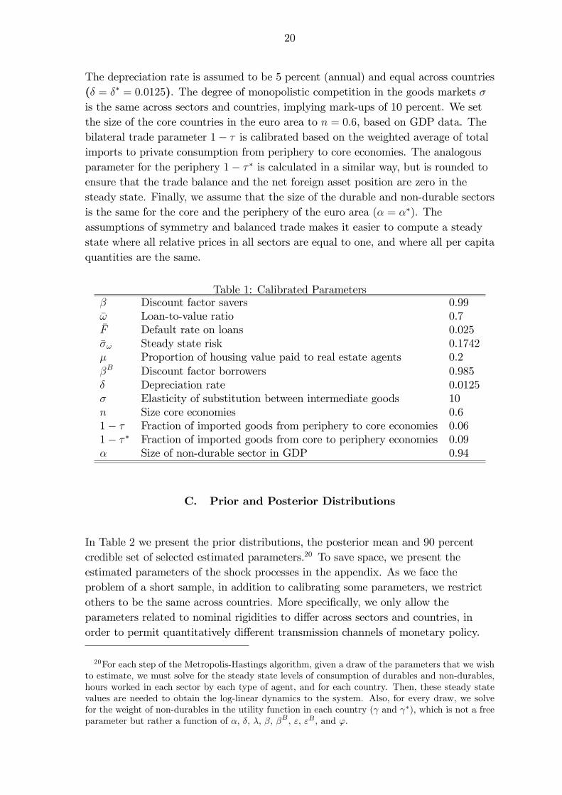
B. Calibrated Parameters

Some parameters are calibrated because the set of observable variables that we usedoes not provide information to estimate them (Table 1). We assume that thediscount factors are the same in both countries (� = �� and �B = �B

�). We set the

discount factor of savers to � = 0:99. The steady state LTV ratio, which alsodetermines the cut-o¤ point for defaulting on a loan, is set to �! = 0:7 and equallyacross countries, according to euro area data such as Gerali et al. (2010). We set thedefault rate on loans, �F (:) to 2:5 percent.18 As a result, the steady state value of therisk shock is ��! = 0:1742: We set the housing agent fee to � = 0:2, which is a valuehigher than that calibrated by Forlati and Lambertini (2010), but lower than therecovery rates for loans estimated for the United States.19 Using these values, thezero-pro�t condition for �nancial intermediaries, and the consumption Eulerequation for borrowers, we obtain a discount factor of borrowers of �B = 0:985.

16Due to the short history of the EMU we face a short time series. We include the years 1995-1998to increase the sample size. During those years most EMU countries were conducting monetarypolicy in a coordinated way.

17See Appendix A for further details on the data set.

18It is di¢ cult to �nd non-perfoming loans for household mortgages only. Therefore, we use non-performing loans as percent of total loans for the euro area between 2000-2011 taken from the WorldBank World Development Indicators database (http://data.worldbank.org/topic/�nancial-sector).

19See Mortgage Bankers Association (2008).

20

The depreciation rate is assumed to be 5 percent (annual) and equal across countries(� = �� = 0:0125). The degree of monopolistic competition in the goods markets �is the same across sectors and countries, implying mark-ups of 10 percent. We setthe size of the core countries in the euro area to n = 0:6, based on GDP data. Thebilateral trade parameter 1� � is calibrated based on the weighted average of totalimports to private consumption from periphery to core economies. The analogousparameter for the periphery 1� � � is calculated in a similar way, but is rounded toensure that the trade balance and the net foreign asset position are zero in thesteady state. Finally, we assume that the size of the durable and non-durable sectorsis the same for the core and the periphery of the euro area (� = ��). Theassumptions of symmetry and balanced trade makes it easier to compute a steadystate where all relative prices in all sectors are equal to one, and where all per capitaquantities are the same.

Table 1: Calibrated Parameters� Discount factor savers 0.99�! Loan-to-value ratio 0.7�F Default rate on loans 0.025��! Steady state risk 0.1742� Proportion of housing value paid to real estate agents 0.2�B Discount factor borrowers 0.985� Depreciation rate 0.0125� Elasticity of substitution between intermediate goods 10n Size core economies 0.61� � Fraction of imported goods from periphery to core economies 0.061� � � Fraction of imported goods from core to periphery economies 0.09� Size of non-durable sector in GDP 0.94

C. Prior and Posterior Distributions

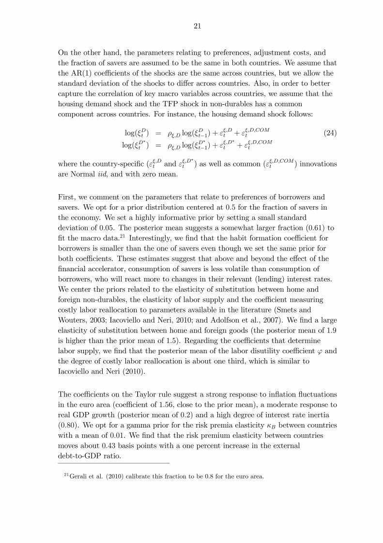
In Table 2 we present the prior distributions, the posterior mean and 90 percentcredible set of selected estimated parameters.20 To save space, we present theestimated parameters of the shock processes in the appendix. As we face theproblem of a short sample, in addition to calibrating some parameters, we restrictothers to be the same across countries. More speci�cally, we only allow theparameters related to nominal rigidities to di¤er across sectors and countries, inorder to permit quantitatively di¤erent transmission channels of monetary policy.

20For each step of the Metropolis-Hastings algorithm, given a draw of the parameters that we wishto estimate, we must solve for the steady state levels of consumption of durables and non-durables,hours worked in each sector by each type of agent, and for each country. Then, these steady statevalues are needed to obtain the log-linear dynamics to the system. Also, for every draw, we solvefor the weight of non-durables in the utility function in each country ( and �), which is not a freeparameter but rather a function of �; �; �; �, �B ; "; "B ; and '.

21

On the other hand, the parameters relating to preferences, adjustment costs, andthe fraction of savers are assumed to be the same in both countries. We assume thatthe AR(1) coe¢ cients of the shocks are the same across countries, but we allow thestandard deviation of the shocks to di¤er across countries. Also, in order to bettercapture the correlation of key macro variables across countries, we assume that thehousing demand shock and the TFP shock in non-durables has a commoncomponent across countries. For instance, the housing demand shock follows:

log(�Dt ) = ��;D log(�Dt�1) + "�;Dt + "�;D;COMt (24)

log(�D�

t ) = ��;D log(�D�

t�1) + "�;D�

t + "�;D;COMt

where the country-speci�c ("�;Dt and "�;D�

t ) as well as common ("�;D;COMt ) innovationsare Normal iid, and with zero mean.

First, we comment on the parameters that relate to preferences of borrowers andsavers. We opt for a prior distribution centered at 0:5 for the fraction of savers inthe economy. We set a highly informative prior by setting a small standarddeviation of 0:05. The posterior mean suggests a somewhat larger fraction (0:61) to�t the macro data.21 Interestingly, we �nd that the habit formation coe¢ cient forborrowers is smaller than the one of savers even though we set the same prior forboth coe¢ cients. These estimates suggest that above and beyond the e¤ect of the�nancial accelerator, consumption of savers is less volatile than consumption ofborrowers, who will react more to changes in their relevant (lending) interest rates.We center the priors related to the elasticity of substitution between home andforeign non-durables, the elasticity of labor supply and the coe¢ cient measuringcostly labor reallocation to parameters available in the literature (Smets andWouters, 2003; Iacoviello and Neri, 2010; and Adolfson et al., 2007). We �nd a largeelasticity of substitution between home and foreign goods (the posterior mean of 1:9is higher than the prior mean of 1:5). Regarding the coe¢ cients that determinelabor supply, we �nd that the posterior mean of the labor disutility coe¢ cient ' andthe degree of costly labor reallocation is about one third, which is similar toIacoviello and Neri (2010).

The coe¢ cients on the Taylor rule suggest a strong response to in�ation �uctuationsin the euro area (coe¢ cient of 1:56, close to the prior mean), a moderate response toreal GDP growth (posterior mean of 0:2) and a high degree of interest rate inertia(0:80). We opt for a gamma prior for the risk premia elasticity �B between countrieswith a mean of 0:01. We �nd that the risk premium elasticity between countriesmoves about 0:43 basis points with a one percent increase in the externaldebt-to-GDP ratio.

21Gerali et al. (2010) calibrate this fraction to be 0:8 for the euro area.

22

Table 2: Prior and Posterior DistributionsPrior Posterior

Parameters Mean SD Mean 90% C.S.� Fraction of savers Beta 0.5 0.05 0.61 [0.53,0.68]" Habit formation savers Beta 0.5 0.15 0.72 [0.65,0.80]"B Habit formation borrowers Beta 0.5 0.15 0.46 [0.26,0.66]' Labor disutility Gamma 1 0.5 0.37 [0.22,0.52]�C Elasticity of subst. between goods Gamma 1.5 0.5 1.90 [1.05,2.67]�L Labor reallocation costs Gamma 1 0.5 0.72 [0.51,0.93] Investment adjustment costs Gamma 2 1 1.75 [1.10,2.35] � Taylor rule reaction to in�ation Normal 1.5 0.1 1.56 [1.41,1.71] y Taylor rule reaction to real growth Gamma 0.2 0.05 0.20 [0.12,0.28] r Interest rate smoothing Beta 0.66 0.15 0.80 [0.77,0.84]�B International risk premium Gamma 0.01 0.005 0.0043 [0.002,0.007]�C Calvo lottery, non-durables Beta 0.75 0.15 0.62 [0.56,0.69]��C Calvo lottery, non-durables Beta 0.75 0.15 0.72 [0.67,0.77]�D Calvo lottery, durables Beta 0.75 0.15 0.64 [0.57,0.72]��D Calvo lottery, durables Beta 0.75 0.15 0.59 [0.52,0.67]�C Indexation, non-durables Beta 0.33 0.15 0.15 [0.02,0.26]��C Indexation, non-durables Beta 0.33 0.15 0.13 [0.02,0.23]�D Indexation, durables Beta 0.33 0.15 0.25 [0.06,0.43]��D Indexation, durables Beta 0.33 0.15 0.43 [0.21,0.68]

Next, we comment on the coe¢ cients regarding nominal rigidities. We opt for Betaprior distributions for Calvo probabilities with a mean of 0:75 (average duration ofprice contracts of four quarters) and standard deviation of 0:15. We set the mean ofthe prior distributions for all indexation parameters to 0:33. This set of priors isconsistent with the survey evidence on price-setting presented in Fabiani et al.(2006). The posterior means for the Calvo lotteries are lower than the prior means,and in all cases prices are reset roughly every three quarters. Overall, theseprobabilities are lower than other studies of the euro area like Smets and Wouters(2003). We also �nd that price indexation is low in all prices and sectors. Onepossible explanation is that we are using a shorter and more recent data set wherein�ation rates are less sticky than in the 1970s and 1980s.

Table C.1 in the appendix presents the prior and posterior distributions for theshock processes. We comment on two results. First, the common innovation tonon-durable technology shocks and durable preference shocks is important, and aswe discuss in the next subsection it is key to obtain cross-country correlations ofsome key macro variables. Second, the mean of the (log) risk shock islog(0:1742) = �1:74. We set a prior standard deviation for the innovation to thehousing risk shock of 0.25 (that is, 25 percent), such that, roughly, the two-standarddeviation prior interval is between -1.25 and -2.25. Given the properties of thelog-normal distribution, this means that the default rate for mortgages rangesbetween 0.04 and 13.6 percent with 95 percent probability. This seems to be an

23

acceptable range for euro area member states.22 The estimates for the quality shockin the periphery are similar to the prior, while in the core there seems to be muchless risk volatility, as re�ected by the posterior.

D. Model Fit and Variance Decomposition

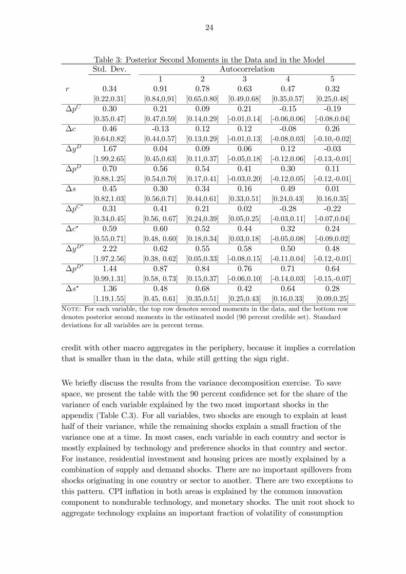
We present the standard deviation and �rst �ve autocorrelations of the observablevariables, and their counterpart in the model implied by the posterior distribution ofthe parameters, to understand how well the model �ts the data. In Table 3, the �rstrow for each entry is the data, the second row is the 90 percent con�dent set impliedby the model estimates. The model does reasonably well in explaining the standarddeviation of all variables in the periphery. However, the model overpredicts thevolatility of prices and quantities in both sectors in the core of the euro area, despitehaving allowed for di¤erent degrees of nominal rigidities, indexation, and di¤erentstandard deviations of shocks. Finally, the model correctly implies that creditgrowth in the periphery is more volatile than in the core. The model also does abetter job in explaining the persistence of variables in the periphery than in thecore, and does a good job in predicting the persistence of interest rates. It slightlyoverpredicts the persistence of CPI in�ation in the periphery, and slightunderpredicts the persistence of residential investment, consumption growth, andhouse prices. In the core, the model has a harder time �tting the lack of persistencein CPI in�ation, residential investment and consumption growth.

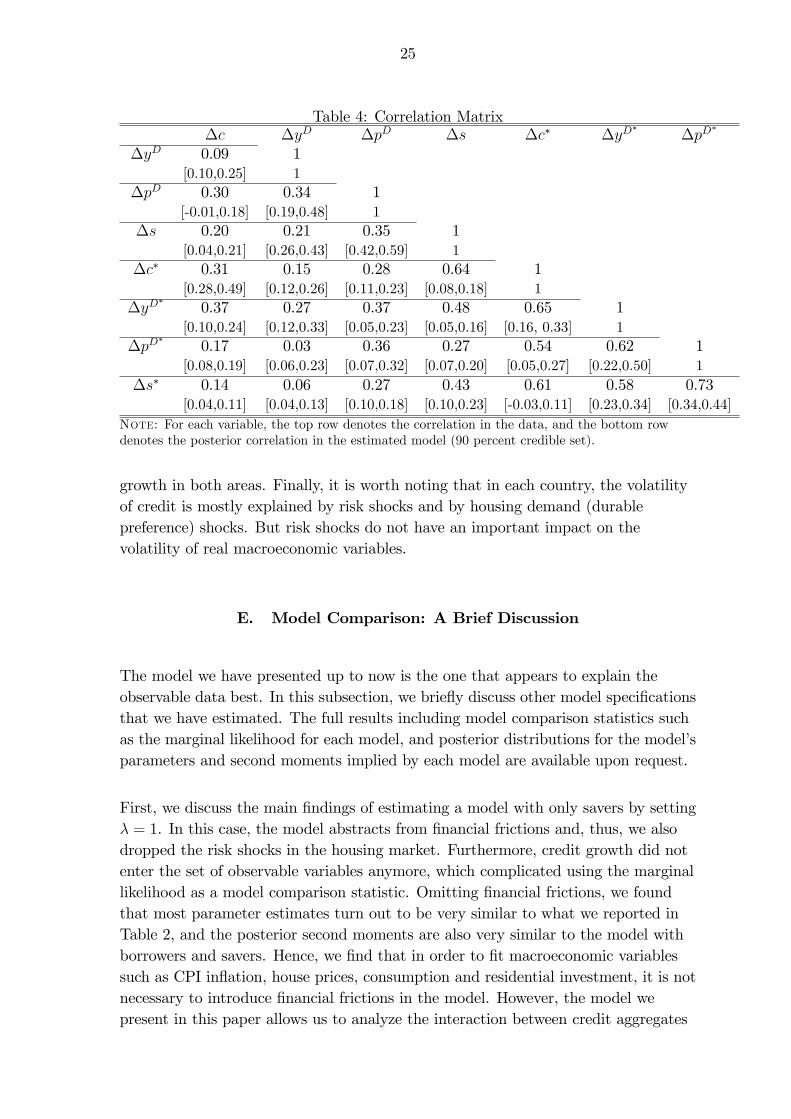
The model captures most of the comovement between main aggregates within andacross countries of the euro area, which is especially important for the design ofoptimal monetary and macroprudential policies. In Table 4 we present thecontemporaneous correlation of selected observable variables in the data and in themodel (90 percent con�dence set).23 Among the successes, we note that the modelexplains the correlation between house prices and residential investment within eacharea well. The model also �ts well the correlation of house price in�ation,consumption growth and residential investment growth across countries. The modelcan explain the comovement between consumption and residential investment in thecore, but fails at explaining the comovement in the periphery. Finally, the modeldoes a good job in explaining the correlation of credit with main macroeconomicvariables in the core. The model does a worse job in explaining the correlation of

22See the World Development Indicators database from the World Bank.

23Table (C.2) in the appendix presents contemporaneous correlation of all observable variables.

24

Table 3: Posterior Second Moments in the Data and in the ModelStd. Dev. Autocorrelation

1 2 3 4 5r 0.34 0.91 0.78 0.63 0.47 0.32

[0.22,0.31] [0.84,0,91] [0.65,0.80] [0.49,0.68] [0.35,0.57] [0.25,0.48]�pC 0.30 0.21 0.09 0.21 -0.15 -0.19

[0.35,0.47] [0.47,0.59] [0.14,0.29] [-0.01,0.14] [-0.06,0.06] [-0.08,0.04]�c 0.46 -0.13 0.12 0.12 -0.08 0.26

[0.64,0.82] [0.44,0.57] [0.13,0.29] [-0.01,0.13] [-0.08,0.03] [-0.10,-0.02]�yD 1.67 0.04 0.09 0.06 0.12 -0.03

[1.99,2.65] [0.45,0.63] [0.11,0.37] [-0.05,0.18] [-0.12,0.06] [-0.13,-0.01]�pD 0.70 0.56 0.54 0.41 0.30 0.11

[0.88,1.25] [0.54,0.70] [0.17,0.41] [-0.03,0.20] [-0.12,0.05] [-0.12,-0.01]�s 0.45 0.30 0.34 0.16 0.49 0.01

[0.82,1.03] [0.56,0.71] [0.44,0.61] [0.33,0.51] [0.24,0.43] [0.16,0.35]�pC

�0.31 0.41 0.21 0.02 -0.28 -0.22

[0.34,0.45] [0.56, 0.67] [0.24,0.39] [0.05,0.25] [-0.03,0.11] [-0.07,0.04]�c� 0.59 0.60 0.52 0.44 0.32 0.24

[0.55,0.71] [0.48, 0.60] [0.18,0.34] [0.03,0.18] [-0.05,0.08] [-0.09,0.02]�yD

�2.22 0.62 0.55 0.58 0.50 0.48

[1.97,2.56] [0.38, 0.62] [0.05,0.33] [-0.08,0.15] [-0.11,0.04] [-0.12,-0.01]�pD

�1.44 0.87 0.84 0.76 0.71 0.64

[0.99,1.31] [0.58, 0.73] [0.15,0.37] [-0.06,0.10] [-0.14,0.03] [-0.15,-0.07]�s� 1.36 0.48 0.68 0.42 0.64 0.28

[1.19,1.55] [0.45, 0.61] [0.35,0.51] [0.25,0.43] [0.16,0.33] [0.09,0.25]Note: For each variable, the top row denotes second moments in the data, and the bottom rowdenotes posterior second moments in the estimated model (90 percent credible set). Standarddeviations for all variables are in percent terms.

credit with other macro aggregates in the periphery, because it implies a correlationthat is smaller than in the data, while still getting the sign right.

We brie�y discuss the results from the variance decomposition exercise. To savespace, we present the table with the 90 percent con�dence set for the share of thevariance of each variable explained by the two most important shocks in theappendix (Table C.3). For all variables, two shocks are enough to explain at leasthalf of their variance, while the remaining shocks explain a small fraction of thevariance one at a time. In most cases, each variable in each country and sector ismostly explained by technology and preference shocks in that country and sector.For instance, residential investment and housing prices are mostly explained by acombination of supply and demand shocks. There are no important spillovers fromshocks originating in one country or sector to another. There are two exceptions tothis pattern. CPI in�ation in both areas is explained by the common innovationcomponent to nondurable technology, and monetary shocks. The unit root shock toaggregate technology explains an important fraction of volatility of consumption

25

Table 4: Correlation Matrix�c �yD �pD �s �c� �yD

��pD

�

�yD 0.09 1[0.10,0.25] 1

�pD 0.30 0.34 1[-0.01,0.18] [0.19,0.48] 1

�s 0.20 0.21 0.35 1[0.04,0.21] [0.26,0.43] [0.42,0.59] 1

�c� 0.31 0.15 0.28 0.64 1[0.28,0.49] [0.12,0.26] [0.11,0.23] [0.08,0.18] 1

�yD�

0.37 0.27 0.37 0.48 0.65 1[0.10,0.24] [0.12,0.33] [0.05,0.23] [0.05,0.16] [0.16, 0.33] 1

�pD�

0.17 0.03 0.36 0.27 0.54 0.62 1[0.08,0.19] [0.06,0.23] [0.07,0.32] [0.07,0.20] [0.05,0.27] [0.22,0.50] 1

�s� 0.14 0.06 0.27 0.43 0.61 0.58 0.73[0.04,0.11] [0.04,0.13] [0.10,0.18] [0.10,0.23] [-0.03,0.11] [0.23,0.34] [0.34,0.44]

Note: For each variable, the top row denotes the correlation in the data, and the bottom rowdenotes the posterior correlation in the estimated model (90 percent credible set).

growth in both areas. Finally, it is worth noting that in each country, the volatilityof credit is mostly explained by risk shocks and by housing demand (durablepreference) shocks. But risk shocks do not have an important impact on thevolatility of real macroeconomic variables.

E. Model Comparison: A Brief Discussion

The model we have presented up to now is the one that appears to explain theobservable data best. In this subsection, we brie�y discuss other model speci�cationsthat we have estimated. The full results including model comparison statistics suchas the marginal likelihood for each model, and posterior distributions for the model�sparameters and second moments implied by each model are available upon request.

First, we discuss the main �ndings of estimating a model with only savers by setting� = 1. In this case, the model abstracts from �nancial frictions and, thus, we alsodropped the risk shocks in the housing market. Furthermore, credit growth did notenter the set of observable variables anymore, which complicated using the marginallikelihood as a model comparison statistic. Omitting �nancial frictions, we foundthat most parameter estimates turn out to be very similar to what we reported inTable 2, and the posterior second moments are also very similar to the model withborrowers and savers. Hence, we �nd that in order to �t macroeconomic variablessuch as CPI in�ation, house prices, consumption and residential investment, it is notnecessary to introduce �nancial frictions in the model. However, the model wepresent in this paper allows us to analyze the interaction between credit aggregates

26

and other macroeconomic variables.

Second, we also estimated our model without common innovations in nondurabletechnology shocks and durable preference shocks across countries. In this case, themodel �t to the data was worse when trying to explain the correlation ofconsumption growth, residential investment growth and house prices acrosscountries. We also experimented with introducing common innovations to othershocks in the model but we found that the estimates of the standard deviations werequite small, and hence did not change the implications of the model for posteriorsecond moments.

Third, instead of assuming that the AR(1) coe¢ cients of the shocks are the sameacross countries, we allowed them to be di¤erent. But this did not improve themodel �t.

Finally, following the results in Christiano, Motto and Rostagno (2013), we alsointroduced news shocks in the housing quality shocks as follows:

log(�!;t) = (1� ��!) log(��!) + ��! log(�!;t�1) +sXp=0

u!;t�p;

for s = 1 to 4. We found that the marginal likelihood favored the model withoutnews shocks and, therefore, we excluded them from the analysis. When weperformed a posterior variance decomposition exercise, we found that laggedinnovations to risk explained a fraction of the variance of credit, but they explaineda very small fraction (less than 1 percent) of the variance of observed realmacroeconomic variables.

IV. Policy Experiments

This section discusses the optimal monetary and macroprudential policy mix for theeuro area. For this purpose, we analyze the performance of di¤erent policy rulesusing the estimated parameter values and shock processes of the previous section.We evaluate aggregate welfare by taking a second order approximation to the utilityfunction of each household and country, and to the equilibrium conditions of themodel, at the posterior mean of the model�s parameters. When policy is conductedat the EMU-wide level, we assume that policy makers maximize the welfare functionof all citizens of the euro area (borrowers and savers in the core and periphery) using

27

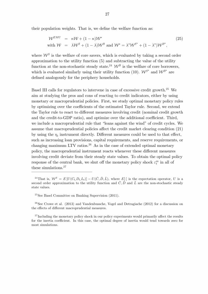
their population weights. That is, we de�ne the welfare function as:

WEMU = nW + (1� n)W� (25)

with W = �WS + (1� �)WB and W� = ��WS� + (1� ��)WB� ;

where WS is the welfare of core savers, which is evaluated by taking a second orderapproximation to the utility function (5) and subtracting the value of the utilityfunction at the non-stochastic steady state.24 WB is the welfare of core borrowers,which is evaluated similarly using their utility function (10). WS� and WB� arede�ned analogously for the periphery households.

Basel III calls for regulators to intervene in case of excessive credit growth.25 Weaim at studying the pros and cons of reacting to credit indicators, either by usingmonetary or macroprudential policies. First, we study optimal monetary policy rulesby optimizing over the coe¢ cients of the estimated Taylor rule. Second, we extendthe Taylor rule to react to di¤erent measures involving credit (nominal credit growthand the credit-to-GDP ratio), and optimize over the additional coe¢ cient. Third,we include a macroprudential rule that �leans against the wind�of credit cycles. Weassume that macroprudential policies a¤ect the credit market clearing condition (21)by using the �t instrument directly. Di¤erent measures could be used to that e¤ect,such as increasing loan provisions, capital requirements, and reserve requirements, orchanging maximum LTV ratios.26 As in the case of extended optimal monetarypolicy, the macroprudential instrument reacts whenever these di¤erent measuresinvolving credit deviate from their steady state values. To obtain the optimal policyresponse of the central bank, we shut o¤ the monetary policy shock "mt in all ofthese simulations.27

24That is, WS = E [U(Ct;Dt;Lt)] � U( �C; �D; �L), where E[�] is the expectation operator, U is asecond order approximation to the utility function and �C; �D and �L are the non-stochastic steadystate values.

25See Basel Committee on Banking Supervision (2011).

26See Crowe et al. (2013) and Vandenbussche, Vogel and Detragiache (2012) for a discussion onthe e¤ects of di¤erent macroprudential measures.

27Including the monetary policy shock in our policy experiments would primarily a¤ect the resultsfor the inertia coe¢ cient. In this case, the optimal degree of inertia would tend towards zero formost simulations.

28

A. Optimal Monetary Policy

A.1 Estimated Taylor Rule

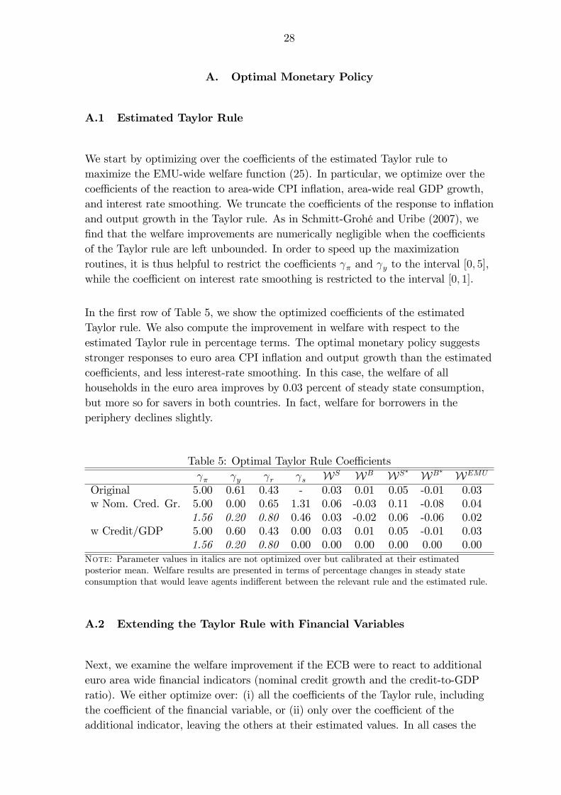
We start by optimizing over the coe¢ cients of the estimated Taylor rule tomaximize the EMU-wide welfare function (25). In particular, we optimize over thecoe¢ cients of the reaction to area-wide CPI in�ation, area-wide real GDP growth,and interest rate smoothing. We truncate the coe¢ cients of the response to in�ationand output growth in the Taylor rule. As in Schmitt-Grohé and Uribe (2007), we�nd that the welfare improvements are numerically negligible when the coe¢ cientsof the Taylor rule are left unbounded. In order to speed up the maximizationroutines, it is thus helpful to restrict the coe¢ cients � and y to the interval [0; 5],while the coe¢ cient on interest rate smoothing is restricted to the interval [0; 1].

In the �rst row of Table 5, we show the optimized coe¢ cients of the estimatedTaylor rule. We also compute the improvement in welfare with respect to theestimated Taylor rule in percentage terms. The optimal monetary policy suggestsstronger responses to euro area CPI in�ation and output growth than the estimatedcoe¢ cients, and less interest-rate smoothing. In this case, the welfare of allhouseholds in the euro area improves by 0.03 percent of steady state consumption,but more so for savers in both countries. In fact, welfare for borrowers in theperiphery declines slightly.

Table 5: Optimal Taylor Rule Coe¢ cients � y r s WS WB WS� WB� WEMU

Original 5.00 0.61 0.43 - 0.03 0.01 0.05 -0.01 0.03w Nom. Cred. Gr. 5.00 0.00 0.65 1.31 0.06 -0.03 0.11 -0.08 0.04

1.56 0.20 0.80 0.46 0.03 -0.02 0.06 -0.06 0.02w Credit/GDP 5.00 0.60 0.43 0.00 0.03 0.01 0.05 -0.01 0.03

1.56 0.20 0.80 0.00 0.00 0.00 0.00 0.00 0.00Note: Parameter values in italics are not optimized over but calibrated at their estimatedposterior mean. Welfare results are presented in terms of percentage changes in steady stateconsumption that would leave agents indi¤erent between the relevant rule and the estimated rule.

A.2 Extending the Taylor Rule with Financial Variables

Next, we examine the welfare improvement if the ECB were to react to additionaleuro area wide �nancial indicators (nominal credit growth and the credit-to-GDPratio). We either optimize over: (i) all the coe¢ cients of the Taylor rule, includingthe coe¢ cient of the �nancial variable, or (ii) only over the coe¢ cient of theadditional indicator, leaving the others at their estimated values. In all cases the

29

coe¢ cients are again truncated to a maximum value of 5. There is some welfareimprovement in reacting to nominal credit growth, but no welfare improvement inreacting to the credit-to-GDP ratio. The optimal response to nominal credit growthis s = 1:31. The same qualitative results hold when we keep the coe¢ cients of theTaylor rule at their estimated values and only optimize over the additionalparameter.

Having monetary policy react to euro area nominal credit growth improves on EMUwelfare. Welfare of savers increases between 0.03 and 0.11 percent of lifetimeconsumption, compared to the estimated Taylor rule. Yet, welfare of borrowersdeclines in both areas. This captures an interesting aspect of our results. Theheterogeneity in the model allows us to identify the winners and losers of di¤erentpolicy regimes in the EMU. We will further examine this result below in the contextof impulse response functions.

B. Macroprudential Regulation

In this subsection, we analyze macroprudential policies that are set countercyclicallyeither at the EMU or at the national level. As in Kannan, Rabanal, and Scott(2012) we introduce a macroprudential tool that aims at a¤ecting the credit marketconditions countercyclically. We assume that the macroprudential rule a¤ects creditsupply and spreads by imposing higher capital requirements, reserve requirements,liquidity ratios or loan-loss provisions. A similar approach is followed by severalmodels analyzed by the BIS to quantify the costs and bene�ts of higher capitalrequirements (see MAG, 2010a,b; and Angelini et al., 2011a).

We assume that �nancial intermediaries are only allowed to lend a fraction 1=�t < 1of their loanable funds. Hence, �nancial intermediaries will pass the costs of notbeing able to lend the full amount of funds to their customers. For instance, in thehome country the macroprudential policy a¤ects the domestic credit marketequilibrium as follows:

�(St +Bt)=�t = (1� �)SBt :

It is useful to rewrite the participation constraint (2) of �nancial intermediaries,using aggregate quantities and the macroprudential instrument as:

RLtRt

=�th

(1� �)R �!at0!dF (!; �!;t)�!at + [1� F (�!at ; �!;t)]

i :A tightening of credit conditions due to macroprudential measures, re�ected in ahigher �t, will increase the spread faced by borrowers. We specify the

30

macroprudential instrument as reacting to an indicator variable (�t):

�t = (�t) � ; ��t = (�

�t ) �� : (26)

We study two main cases. In each country the macroprudential instrument reactsto: (i) nominal credit growth, or (ii) the credit-to-GDP ratio. For both cases, theparameters � and

�� are either allowed to be di¤erent, or are forced to be the same

in the union. In all cases, the indicator reacts to deviations from steady state values.

B.1 Regulation at the EMU-Level

We analyze the optimal policy regime consisting of the estimated Taylor ruletogether with national macroprudential rules (26) and optimize over the parametersof these three rules in order to maximize the welfare criterion (25). In this scenario,monetary policy reacts to union-wide developments, while macroprudential policyresponds to domestic developments in each country. The coe¢ cients of these policyrules are jointly decided to maximize welfare at the European level. Since we allowthe macroprudential rule to a¤ect credit variables directly, we no longer include thereaction to credit in the Taylor rule. Therefore, the macroprudential instrument canbe viewed as an alternative to having monetary policy react to indicators beyondCPI in�ation and output growth. In this sense, we study the Svensson (2012)suggestion that monetary policy should be in charge of price stability whilemacroprudential policy should address �nancial stability.

In Table 6 we consider the following combinations of cases: (i) macroprudentialregulation either reacts to nominal credit growth or the credit-to-GDP ratio, (ii) thecoe¢ cients of the Taylor rule are the estimated ones, or are optimized with theparameters of the macroprudential rule, and (iii) the coe¢ cients of themacroprudential policies are allowed to change across countries, or are restricted tobe the same.

Several interesting results arise from this exercise. First of all, in some cases thereare winners and losers of introducing macroprudential policies. The only policy thatimproves welfare for each type of agent, yet it does not maximize EMU-wide welfare,is to have macroprudential policy react to nominal credit growth. In this regime, allhouseholds experience increases in welfare between 0.01 and 0.19 percent of lifetimeconsumption, and there are no big numerical di¤erences in welfare if we impose therestriction that the coe¢ cients are the same across countries. For both cases, thereis a further welfare improvement at the EMU level with respect to the regime withoptimized Taylor rule coe¢ cients only. Second, the policy that delivers higher

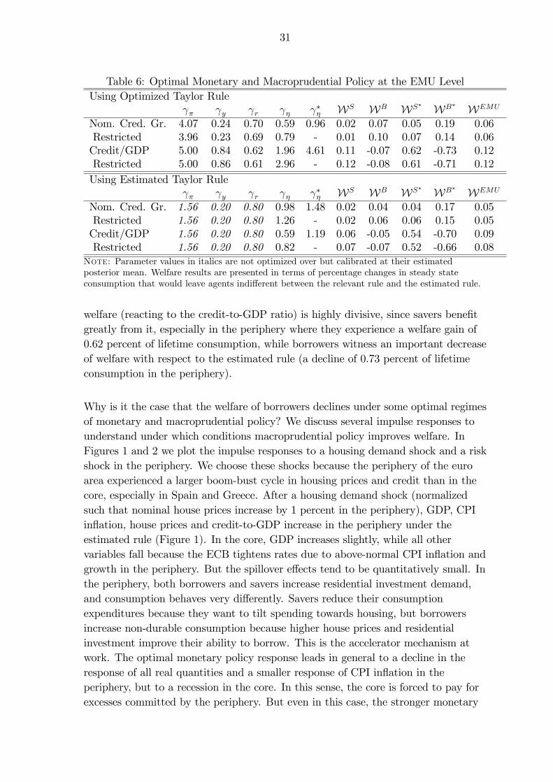
31

Table 6: Optimal Monetary and Macroprudential Policy at the EMU LevelUsing Optimized Taylor Rule

� y r � �� WS WB WS� WB� WEMU

Nom. Cred. Gr. 4.07 0.24 0.70 0.59 0.96 0.02 0.07 0.05 0.19 0.06Restricted 3.96 0.23 0.69 0.79 - 0.01 0.10 0.07 0.14 0.06Credit/GDP 5.00 0.84 0.62 1.96 4.61 0.11 -0.07 0.62 -0.73 0.12Restricted 5.00 0.86 0.61 2.96 - 0.12 -0.08 0.61 -0.71 0.12Using Estimated Taylor Rule

� y r � �� WS WB WS� WB� WEMU

Nom. Cred. Gr. 1.56 0.20 0.80 0.98 1.48 0.02 0.04 0.04 0.17 0.05Restricted 1.56 0.20 0.80 1.26 - 0.02 0.06 0.06 0.15 0.05Credit/GDP 1.56 0.20 0.80 0.59 1.19 0.06 -0.05 0.54 -0.70 0.09Restricted 1.56 0.20 0.80 0.82 - 0.07 -0.07 0.52 -0.66 0.08

Note: Parameter values in italics are not optimized over but calibrated at their estimatedposterior mean. Welfare results are presented in terms of percentage changes in steady stateconsumption that would leave agents indi¤erent between the relevant rule and the estimated rule.

welfare (reacting to the credit-to-GDP ratio) is highly divisive, since savers bene�tgreatly from it, especially in the periphery where they experience a welfare gain of0.62 percent of lifetime consumption, while borrowers witness an important decreaseof welfare with respect to the estimated rule (a decline of 0.73 percent of lifetimeconsumption in the periphery).

Why is it the case that the welfare of borrowers declines under some optimal regimesof monetary and macroprudential policy? We discuss several impulse responses tounderstand under which conditions macroprudential policy improves welfare. InFigures 1 and 2 we plot the impulse responses to a housing demand shock and a riskshock in the periphery. We choose these shocks because the periphery of the euroarea experienced a larger boom-bust cycle in housing prices and credit than in thecore, especially in Spain and Greece. After a housing demand shock (normalizedsuch that nominal house prices increase by 1 percent in the periphery), GDP, CPIin�ation, house prices and credit-to-GDP increase in the periphery under theestimated rule (Figure 1). In the core, GDP increases slightly, while all othervariables fall because the ECB tightens rates due to above-normal CPI in�ation andgrowth in the periphery. But the spillover e¤ects tend to be quantitatively small. Inthe periphery, both borrowers and savers increase residential investment demand,and consumption behaves very di¤erently. Savers reduce their consumptionexpenditures because they want to tilt spending towards housing, but borrowersincrease non-durable consumption because higher house prices and residentialinvestment improve their ability to borrow. This is the accelerator mechanism atwork. The optimal monetary policy response leads in general to a decline in theresponse of all real quantities and a smaller response of CPI in�ation in theperiphery, but to a recession in the core. In this sense, the core is forced to pay forexcesses committed by the periphery. But even in this case, the stronger monetary

32

policy stance on CPI in�ation and growth does not contain accelerator e¤ects toreally a¤ect credit-to-GDP ratio in the periphery. In order to achieve this, the use ofmacroprudential measures is necessary: For this reason, we now add themacroprudential rule that reacts to the credit-to-GDP ratio optimally (Table 6). Asa result, credit-to-GDP in the periphery increases to a lesser extent, there are lessaccelerator e¤ects, and hence the stance of monetary policy can be softened in theEMU as a whole after several periods. Overall, the regime of optimal monetary plusmacroprudential policy delivers more stability on all real quantities in the periphery,and this improves welfare. However, this last regime cannot fully o¤set the negativespillover e¤ects from the periphery to the core borrowers. Similar qualitative resultswould hold if the housing boom was in the core, but with core savers and borrowersbene�tting more from stability using macroprudential policies.

A negative risk shock in the periphery has very similar e¤ects on most variables inthe periphery as the housing demand shock. When risk declines, lending-depositspreads falls in the periphery (the shock is normalized such that spreads decline by25 basis points on an annualized basis), triggering an increase in the credit-to-GDPratio. Under the estimated rule, consumption and residential investment byborrowers increase in the periphery, but that of savers decline. In the aggregate,GDP increases in the periphery, and increased demand by borrowers also increasesGDP in the core, mostly through the net exports channel. However, higher in�ationleads to in increase of interest rates that makes spending fall for both borrowers andsavers in the core. The optimal monetary policy tries to stabilize CPI in�ation byincreasing interest rates, which leads to reductions of spending for all otherhouseholds in the EMU, and a recession and de�ation in the core. As in the case ofthe housing demand shock, optimal monetary policy cannot do much to o¤set theaccelerator e¤ects, while the use of macroprudential tools delivers overall stabilityand takes the pressure of the EMU-wide interest rate. If the risk shock a¤ects thecore, it will have a similar impact on core variables as the one described here forperiphery variables, and vice versa.

When does the use of macroprudential tools lead to inferior welfare outcomes? InFigure 3 we plot the e¤ect of an innovation to the EMU-wide (one standarddeviation) permanent technology shock. In this case, macroprudential policiesincrease the countercyclicality of the lending-deposit premium, increasing thevolatility of borrower-speci�c variables and reducing their welfare. When apermanent technology hits the economy, this increases the level of real variablespermanently (however, growth rates and transformed variables remain stationary).Since this is a permanent shock and both economies are quite symmetric, the e¤ectsare similar in both areas of the EMU. In particular, consumption by savers smoothlymoves to the new level, while residential investment by borrowers is a bit morevolatile. CPI in�ation falls in both areas due to the decline in real marginal costs,while nominal and real house prices increase. Interestingly, under the estimated rule,

33

credit-to-GDP falls, even though both quantities increase, but the lending-depositspread declines only slightly, re�ecting minimal movements in the LTV ratios.Hence, the main variables for borrowers move similarly to that of savers. Optimalmonetary policy aims at bringing CPI in�ation back to target so that the ECB cutsnominal interest rates and CPI in�ation falls to a lesser extent. Moreover, most realvariables display less volatility and a faster transition to their new steady statevalues. What is the problem of using macroprudential policies in this set-up? In thiscase, the macroprudential policy aims at addressing the decline of the credit-to-GDPratio by allowing banks to lend more. As a result, the credit-to-GDP ratio falls bymuch less and the lending-deposit rate becomes more volatile. This generates ahigher countercyclical response of the lending rate, which �nally increases thevolatility of consumption and residential investment by borrowers. Because theyhave access to cheap credit, borrowers spend more and supply less labor, makinghours worked for borrowers also more volatile, which further adds to their welfarecost. On the other hand, savers still face a smooth consumption and investmentplan. By picking up the labor slack left by borrowers their overall labor supply isless volatile, contributing to their welfare increase.

Hence, in a model with a micro-founded behavior of the lending-deposit spread, andthe welfare function, we �nd a similar result to Kannan et al. (2012), who usesad-hoc lending-deposit spreads and welfare functions. Macroprudential policies that"lean against the wind" improve welfare when it is optimal to reduce thecountercyclical behavior of the spread, as is the case of housing demand or riskshocks. However, under technology shocks, mechanical responses to thecredit-to-GDP ratio will actually increase the countercyclical behavior of the spread,leading to an increased volatility of spending by borrowers, and hurting theirwelfare, even when the impact on aggregate variables such as real GDP or CPIin�ation is quantitatively very small.

We conduct an additional robustness result by looking at the optimal response ofmonetary and macroprudential policies if the policy makers were able to identify thesource of the shock. To that end, we simulate the model with either technologyshocks only (including all sectors and countries and the unit root shock), preferenceshocks only (including all countries and sectors), and �nancial shocks only(including the housing quality risk shock and the risk premium shock acrosscountries). The optimal responses are quite di¤erent when the monetary andmacroprudential authorities can identify the source of the shock (Table 7). A keydi¤erence, that we identi�ed in the impulse response analysis, is that the optimalmacroprudential response to any credit aggregate becomes zero under the optimizedTaylor rule and technology shocks. As we already saw from Figure 3, includingmacroprudential policies when technology shocks are present reduced welfare ofborrowers by inducing too much volatility in the lending-deposit spread. However,when �nancial shocks hit the economy, the optimal macroprudential responses calls

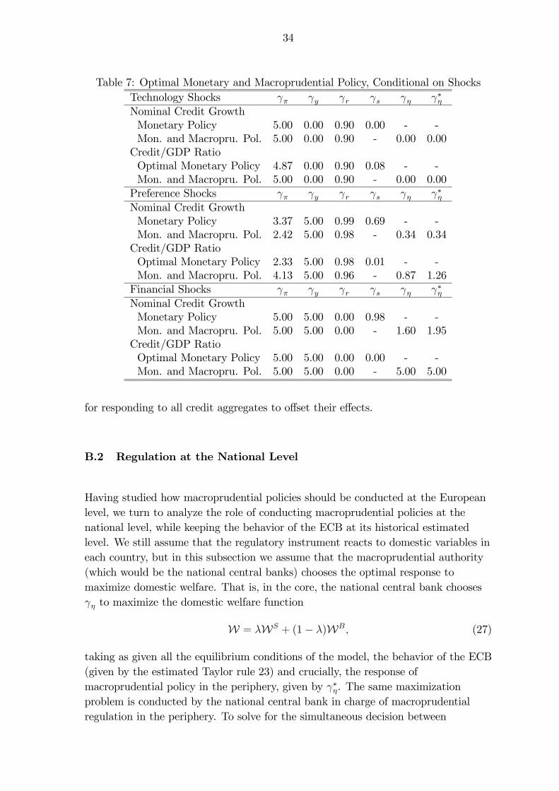
34

Table 7: Optimal Monetary and Macroprudential Policy, Conditional on ShocksTechnology Shocks � y r s � ��Nominal Credit GrowthMonetary Policy 5.00 0.00 0.90 0.00 - -Mon. and Macropru. Pol. 5.00 0.00 0.90 - 0.00 0.00Credit/GDP RatioOptimal Monetary Policy 4.87 0.00 0.90 0.08 - -Mon. and Macropru. Pol. 5.00 0.00 0.90 - 0.00 0.00Preference Shocks � y r s � ��Nominal Credit GrowthMonetary Policy 3.37 5.00 0.99 0.69 - -Mon. and Macropru. Pol. 2.42 5.00 0.98 - 0.34 0.34Credit/GDP RatioOptimal Monetary Policy 2.33 5.00 0.98 0.01 - -Mon. and Macropru. Pol. 4.13 5.00 0.96 - 0.87 1.26Financial Shocks � y r s � ��Nominal Credit GrowthMonetary Policy 5.00 5.00 0.00 0.98 - -Mon. and Macropru. Pol. 5.00 5.00 0.00 - 1.60 1.95Credit/GDP RatioOptimal Monetary Policy 5.00 5.00 0.00 0.00 - -Mon. and Macropru. Pol. 5.00 5.00 0.00 - 5.00 5.00

for responding to all credit aggregates to o¤set their e¤ects.

B.2 Regulation at the National Level

Having studied how macroprudential policies should be conducted at the Europeanlevel, we turn to analyze the role of conducting macroprudential policies at thenational level, while keeping the behavior of the ECB at its historical estimatedlevel. We still assume that the regulatory instrument reacts to domestic variables ineach country, but in this subsection we assume that the macroprudential authority(which would be the national central banks) chooses the optimal response tomaximize domestic welfare. That is, in the core, the national central bank chooses � to maximize the domestic welfare function

W = �WS + (1� �)WB; (27)

taking as given all the equilibrium conditions of the model, the behavior of the ECB(given by the estimated Taylor rule 23) and crucially, the response ofmacroprudential policy in the periphery, given by ��. The same maximizationproblem is conducted by the national central bank in charge of macroprudentialregulation in the periphery. To solve for the simultaneous decision between

35

macroprudential authorities in the core and in the periphery, we compute the bestresponse functions for each country as a function of the response in the othercountry. Then, the Nash equilibrium is given by the intersection of the two bestresponses.

Two results are worth emphasizing. First, the best response functions of the nationalmacroprudential policies are �at, i.e. the optimal response in choosing the coe¢ cient � in the core is independent of the choice of the macroprudential instrument in theperiphery, and vice versa. We show an example when both regulators react tonominal credit growth in Figure 4. Second, the optimal coe¢ cients whenmacroprudential policy is set at the national level are numerically very close to thecase where macroprudential policies are set at the EMU-level maximizing jointwelfare (presented in Table 6 when the ECB follows the estimated rule).

V. Conclusions

In this paper, we have studied the optimal mix of monetary and macroprudentialpolicies in an estimated DSGE model of the euro area. We have found that in avariety of scenarios and calibrations, the introduction of a macroprudential rulewould help in reducing macroeconomic volatility and hence in improving EMU-widewelfare. At the same time, we have observed that macroprudential policies �lend ahand�to monetary policy by reducing accelerator e¤ects and thus, requiring smallerresponses of the nominal interest. We have also shown that the e¤ects ofmacroprudential regulations can a¤ect savers and borrowers di¤erently. The policythat improves welfare in the EMU the most - which would be to havemacroprudential policies respond to the credit-to-GDP ratio - reduces the welfare ofborrowers by inducing a too countercyclical response of the lending-deposit spread.Improving welfare for all citizens in the EMU will only be achieved, ifmacroprudential policies respond to nominal credit growth. Finally, we have alsofound that there are no negative spillover e¤ects of regulation from one memberstate to another. Having macroprudential policies set at the national or EMU widelevels will therefore not change the outcome.

36

References

Adolfson, M., Laseen, S., Lindé, J., and M. Villani, 2007. Bayesian Estimation ofan Open Economy DSGE Model with Incomplete Pass-Through. Journal ofInternational Economics, Vol. 72(2), pp. 481-511.

An, S. and F. Schorfheide, 2007. Bayesian Analysis of DSGE Models. EconometricReviews, Vol. 26(2-4), pp. 113-172.

Angelini, P., Clerc, L., Cúrdia, V., Gambacorta, L., Gerali, A., Locarno, A., Motto,R., Roeger, W., Van den Heuvel, S. and J. Vlcek, 2011a. BASEL III:Long-term Impact on Economic Performance and Fluctuations. BIS WorkingPapers No. 338.

Angelini, P., Neri, S., and F. Panetta, 2011b. Monetary and MacroprudentialPolicies. Temi di discussione (Economic working papers) No. 801, Bank ofItaly, Economic Research Department.

Bank of England, 2009. The Role of Macroprudential Policies. Discussion Paper.

Basel Committee on Banking Supervision, 2011. Basel III: A Global RegulatoryFramework for More Resilient Banks and Banking Systems.

Bean, C. , Paustian, M., Penalver, A. and T. Taylor, 2010. Monetary Policy afterthe Fall. Paper presented at the Federal Reserve Bank of Kansas City AnnualConference, Jackson Hole, Wyoming, 16 September 2010.

Beau, D., Clerc, L. and B. Mojon, 2012. Macro-Prudential Policy and the Conductof Monetary Policy. Working papers No. 390, Banque de France.

Bernanke, B., Gertler, M., and S. Gilchrist, 1998. The Financial Accelerator in aQuantitative Business Cycle Framework. NBER Working Paper No. 6455.

Bianchi, J. and E. Mendoza, 2011. Overborrowing, Financial Crises and�Macro-prudential�Policy. IMF Working Paper No. 11/24.

Blanchard, O, Dell�Ariccia, G., and P. Mauro, 2010. Rethinking MacroeconomicPolicy. Journal of Money, Credit and Banking, Vol. 42(s1), pp. 199�215.

Borio, C. and I. Shim, 2008. What can (Macro-)Prudential Policy Do to SupportMonetary Policy?. Bank for International Settlements Working Paper No. 242.

Brzoza-Brzezina, M., Kolasa, M., and K. Makarski, 2013. Macroprudential Policyand Imbalances in the Euro Area. National Bank of Poland.Working PaperNo. 138.

Calvo, G., 1983. Staggered Prices in a Utility Maximizing Framework. Journal of

37

Monetary Economics, Vol. 12(3), pp. 383-398.

Christiano, L., Eichenbaum, M., and C. Evans, 2005. Nominal Rigidities and theDynamic E¤ects of a Shock to Monetary Policy. Journal of Political Economy,Vol. 113(1), pp. 1-45.

Christiano, L., Motto, R., and M. Rostagno, 2013. Risk Shocks. NBER WorkingPaper No. 18682.

Claessens, S., Kose, A., and M. E. Terrones, 2008. What Happens DuringRecessions, Crunches and Busts?. IMF Working Paper No. 08/274.

Crowe, C., Dell�Ariccia, G., Igan, D., and P. Rabanal, 2013. How to Deal with RealEstate Booms: Lessons from Country Experiences. Journal of FinancialStability,.Vol. 9(3), pp. 300-319.

European Central Bank, 2009. Housing Finance in the Euro Area. ECB OccasionalPaper No. 101.

Fabiani, S., M. Druant, I. Hernando, C. Kwapil, B. Landau, C. Loupias, F.Martins, T. Mathä, R. Sabbatini, H. Stahl, and A. Stokman, 2006. WhatFirms�Surveys Tell Us About Price-Setting Behavior in the Euro Area.International Journal of Central Banking, Vol. 2(3), pp. 3-47.

Forlati, C., and L. Lambertini, 2011. Risky Mortgages in a DSGE Model.International Journal of Central Banking, Vol. 7(1), pp. 285-336.

Galati, G. and R. Moessner, 2012. Macroprudential Policy - A Literature Review.forthcoming in Journal of Economic Surveys.

Gerali, A., Neri, S., Sessa, L., and F. Signoretti, 2010. Credit and Banking in aDSGE Model of the Euro Area. Journal of Money, Credit and Banking, Vol.42(s1), pp. 107-141.

Goyal, R., Koeva Brooks, P., Pradhan, M., Tressel, T., Dell�Ariccia, G., Leckow,R., and C. Pazarbasioglu, 2013. A Banking Union for the Euro Area. IMFSta¤ Discussion Note 13/01.

Gruss, B., and S. Sgherri, 2009. The Volatility Costs of Procyclical LendingStandards: An Assessment Using a DSGE Model. IMF Working Paper No.09/35.

Iacoviello, M., 2005. House Prices, Borrowing Constraints and Monetary Policy inthe Business Cycle. American Economic Review, Vol. 95(3), pp. 739-764.

Iacoviello M., and S. Neri, 2010. The Role of Housing Collateral in an EstimatedTwo-Sector Model of the U.S. Economy. American Economic Journal:

38

Macroeconomics, Vol. 2(2), pp. 125-164.

International Monetary Fund, 2009. Lessons from Asset Price Fluctuations forMonetary Policy. Chapter 3 of World Economic Outlook, October 2009,International Monetary Fund., Washington, DC.

International Monetary Fund, 2012. Dealing with Household Debt. Chapter 3 ofWorld Economic Outlook, April 2012, International Monetary Fund.,Washington, DC.

Kaminsky, G. and C. M. Reinhart, 1999. The Twin Crises: The Causes of Bankingand Balance-of-Payments Problems. American Economic Review, Vol. 89(3),pp. 473-500.

Kannan, P., Rabanal, P., and A. Scott, 2012. Monetary and MacroprudentialPolicy Rules in a Model with House Price Booms. The B.E. Journal ofMacroeconomics, Vol. 12(1), pp. 1-44.

Lambertini, L., Mendicino, C., and M.T. Punzi, 2011. Leaning Against Boom-BustCycles in Credit and Housing Prices: Monetary and Macroprudential Policy.Bank of Portugal Working Paper No. 2011/08.

Macroeconomic Assessment Group (MAG), 2010a. Assessing the MacroeconomicImpact of the Transition to Stronger Capital and LiquidityRequirements� Interim Report. Group established by the Financial StabilityBoard and the Basel Committee on Banking Supervision, August.

Macroeconomic Assessment Group (MAG), 2010b. Assessing the MacroeconomicImpact of the Transition to Stronger Capital and LiquidityRequirements� Final Report. Group established by the Financial StabilityBoard and the Basel Committee on Banking Supervision, December.

Mortgage Banker Association, 2008. Lenders�Cost of Foreclosure, Policy PaperCongressional Education Series Brie�ng.

Roger, S. and J. Vlcek, 2011. Macroeconomic Costs of Higher Bank Capital andLiquidity Requirements. IMF Working Paper No. 11/103.

Schmitt-Grohé, S. and M. Uribe, 2003. Closing Small Open Economy Models.Journal of International Economics, Vol. 61(1), pp. 163-185.

Schmitt-Grohé, S. and M. Uribe, 2007. Optimal, Simple, and ImplementableMonetary and Fiscal Rules. Journal of Monetary Economics, Vol. 54(6), pp.1702-1725.

Smets, F. and R. Wouters, 2003. An Estimated Stochastic Dynamic GeneralEquilibrium Model for the Euro Area. Journal of the European Economic

39

Association, Vol. 1(5), pp. 1123-1175.

Sorensen, C., and J. Lichtenberger, 2007. Mortgage Interest Rate Dispersion in theEuro Area. ECB Working Paper No. 733.

Suh, H., 2012. Macroprudential Policy: Its E¤ects and Relationship to MonetaryPolicy. Federal Reserve Bank of Philadelphia Working Paper No. 12-28.

Svensson, L., 2012. Comment on Michael Woodford: "In�ation Targeting andFinancial Stability". Sveriges Riksbank Economic Review 2012:1, pp. 33-39.

Unsal, F., 2011. Capital Flows and Financial Stability: Monetary Policy andMacroprudential Responses. IMF Working Paper No. 11/189.

Vandenbussche, J., Vogel, U. and E. Detragiache, 2012. Macroprudential Policiesand Housing Prices� A New Database and Empirical Evidence for Central,Eastern, and Southeastern Europe. IMF Working Paper No. 12/303.

Zhang, L., 2009. Bank Capital Regulation, the Lending Channel and BusinessCycles. Discussion Paper Series 1: Economic Studies No. 2009,33, DeutscheBundesbank, Research Centre.

40

Appendix

A Data and Sources

Since we distinguish between two regions of the euro area, data for the core isobtained by aggregating data for France and Germany, while for the periphery datafor Greece, Ireland, Italy, Portugal, and Spain are combined. The aggregation isdone by computing weighted averages taking into account the relative economic sizeof the countries (measured by nominal GDP). Some of the series start later than1995q4 or end earlier than 2011q4. If this is the case, aggregation for these quartersonly takes into account available data, while weights are adjusted accordingly. Alldata is seasonally adjusted in case this has not been done by the original source.Finally, all data is demeaned.

In�ation: Quarter on quarter log di¤erences in the Harmonized Index of ConsumerPrices (HICP), not seasonally adjusted by the source. Source: ECB.

Change in House Price Data: Quarter on quarter log di¤erences in real housingprices. All data, except for Greece and Portugal, is provided by the OECD. Greekand Portuguese data is provided by the BIS. All OECD data is seasonally adjustedby the source, while BIS data is not. Portuguese data is only available on a monthlybasis and is transformed to a quarterly frequency by taking averages. Data for Italyalready ends in 2011q3.

Real Private Consumption: Final consumption of households and nonpro�tinstitutions serving households (NPISH), seasonally adjusted by the source. Source:Eurostat.

Real Residential Investment: Gross �xed capital formation in construction workfor housing, seasonally adjusted by the source. Data for Ireland is only available onan annual basis while data for Greece is only available from 2000 onwards on anannual basis. Both data is interpolated to obtain quarterly values. Source: Eurostat.

ECB Interest Rate: 3-month Euribor, Source: ECB.

Household Outstanding Debt: Data seasonally adjusted by the source. Data forGreece starts in 1997q4, for Ireland in 2002q1, and for Italy in 1997q1. Source:Eurostat.

Nominal GDP for computing the weights used in the aggregation is taken from the

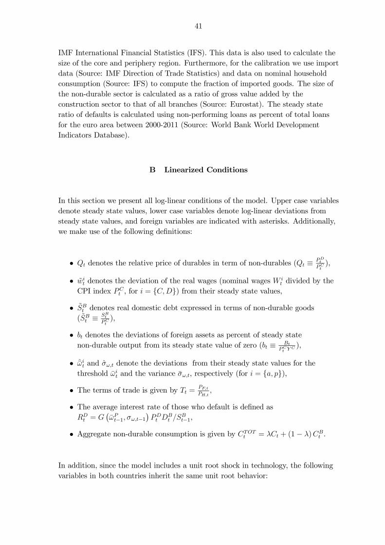
41

IMF International Financial Statistics (IFS). This data is also used to calculate thesize of the core and periphery region. Furthermore, for the calibration we use importdata (Source: IMF Direction of Trade Statistics) and data on nominal householdconsumption (Source: IFS) to compute the fraction of imported goods. The size ofthe non-durable sector is calculated as a ratio of gross value added by theconstruction sector to that of all branches (Source: Eurostat). The steady stateratio of defaults is calculated using non-performing loans as percent of total loansfor the euro area between 2000-2011 (Source: World Bank World DevelopmentIndicators Database).

B Linearized Conditions

In this section we present all log-linear conditions of the model. Upper case variablesdenote steady state values, lower case variables denote log-linear deviations fromsteady state values, and foreign variables are indicated with asterisks. Additionally,we make use of the following de�nitions:

� Qt denotes the relative price of durables in term of non-durables (Qt � PDtPCt),

� ~wit denotes the deviation of the real wages (nominal wages Wit divided by the

CPI index PCt , for i = fC;Dg) from their steady state values,

� ~SBt denotes real domestic debt expressed in terms of non-durable goods( ~SBt �

SBtPCt),

� bt denotes the deviations of foreign assets as percent of steady statenon-durable output from its steady state value of zero (bt � Bt

PCt YC ),

� �̂!it and �̂!;t denote the deviations from their steady state values for thethreshold �!it and the variance ��!;t, respectively (for i = fa; pg),

� The terms of trade is given by Tt = PF;tPH;t

;

� The average interest rate of those who default is de�ned asRDt = G

��!Pt�1; �!;t�1

�PDt D

Bt =S

Bt�1,

� Aggregate non-durable consumption is given by CTOTt = �Ct + (1� �)CBt .

In addition, since the model includes a unit root shock in technology, the followingvariables in both countries inherit the same unit root behavior:

42

� consumption of non-durables (by agent and aggregate, including domesticallyproduced and imported): Ct; CBt ; C

TOTt , CH;t; CF;t,

� residential investment and the housing stock of both borrowers and savers: It,IBt ; Dt; D

Bt ;

� real wages in both sectors: WCt , and W

Dt ;

� the production of durable and non-durable goods: Y Ct and Y D

t ; and real GDPYt;

� and real credit ~SBt .

Hence, we normalize all these real variables by the level of technology Zt. For thesevariables, lower case variables denote deviations from steady state values ofnormalized variables. That is, ct = log(Ct=Zt)� log(C=Z) and so on. Foreigncountry variables are normalized in the same way. For instance,c�t = log(C

�t =Zt)� log(C�=Z).

Home Country

From the optimal decision by savers we get the following:28

qt + �Ct �ct � "(ct�1 � "zt )

1� "+ (it � it�1 + "zt ) = Et%t+1 + � (Etit+1 � it); (B.1)

where = z"(:) and %t is the normalized Lagrange multiplier associated with thelaw of motion of the housing stock (9) for savers, and

[1� �(1� �)] (�Dt � dt) = %t � �(1� �)Et%t+1; (B.2)

"(�ct + "zt ) = Et�ct+1 � (1� ")(rt + Et��Ct+1 � Et�p

Ct+1): (B.3)

The labor supply schemes to the non-durable and durable sectors are:

[('� �L)�+ �L] lCt + ('� �L)(1� �)lDt = ~wCt + �Ct �

ct � "(ct�1 � "zt )

1� "; (B.4)

[('� �L)(1� �) + �L] lDt + ('� �L)�l

Ct = ~wDt + �Ct �

ct � "(ct�1 � "zt )

1� ": (B.5)

28Since all households behave the same way, we henceforth drop the j superscript.

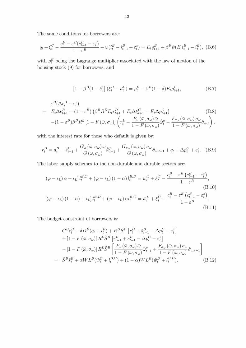
43

The same conditions for borrowers are:

qt+ �Ct �

cBt � "B(cBt�1 � "zt )

1� "B+ (iBt � iBt�1 + "zt ) = Et%

Bt+1 + �

B (EtiBt+1� iBt ); (B.6)

with %Bt being the Lagrange multiplier associated with the law of motion of thehousing stock (9) for borrowers, and

�1� �B(1� �)

�(�Dt � dBt ) = %Bt � �B(1� �)Et%

Bt+1; (B.7)

"B(�cBt + "zt )

= Et�cBt+1 � (1� "B)

��BRDEtr

Dt+1 + Et��

Ct+1 � Et�p

Ct+1

�(B.8)

�(1� "B)�BRL [1� F (�!; �!)]

�rLt �

F! (�!; �!) �!

1� F (�!; �!)�̂!at �

F�! (�!; �!)�!1� F (�!; �!)

�̂!;t

�;

with the interest rate for those who default is given by:

rDt = dBt � ~sBt�1 +G! (�!; �!) �!

G (�!; �!)�̂!pt�1 +

G�! (�!; �!)�!G (�!; �!)

�̂!;t�1 + qt +�pCt + "zt : (B.9)

The labor supply schemes to the non-durable and durable sectors are:

[('� �L)�+ �L] lB;Ct + ('� �L) (1� �) lB;Dt = ~wCt + �Ct �

cBt � "B�cBt�1 � "zt

�1� "B

;

(B.10)

[('� �L) (1� �) + �L] lB;Dt + ('� �L)�l

B;Ct = ~wDt + �Ct �

cBt � "B�cBt�1 � "zt

�1� "B

:

(B.11)

The budget constraint of borrowers is:

CBcBt + �DB(qt + iBt ) +RD ~SB�rDt + ~s

Bt�1 ��pCt � "zt

�+ [1� F (�!; �!)]R

L ~SB�rLt�1 + ~s

Bt�1 ��pCt � "zt

�� [1� F (�!; �!)]R

L ~SB�F! (�!; �!) �!

1� F (�!; �!)�̂!pt�1 +

F�! (�!; �!)�!1� F (�!; �!)

�̂!;t�1

�= ~SB~sBt + �WLB( ~wCt + lB;Ct ) + (1� �)WLB( ~wDt + lB;Dt ): (B.12)

44

The lending rate for borrowers is determined by the participation constraint of�nancial intermediaries:

1

�~SB�rt + ~s

Bt + �t

�= (1� �)DBG (�!; �!)

�G! (�!; �!) �!

G (�!; �!)�̂!at +

G�! (�!; �!)�!G (�!; �!)

�̂!;t

�+(1� �)DBG (�!; �!)

�Etqt+1 + Etd

Bt+1 + Et�p

Ct+1

�(B.13)

+ [1� F (�!; �!)]RL ~SB

�rLt + ~s

Bt �

F! (�!; �!) �!

1� F (�!; �!)�̂!at �

F�! (�!; �!)�!1� F (�!; �!)

�̂!;t

�:

The ex-ante and ex-post default threshold is:

�̂!at + Et�qt+1 + dBt+1

�= rLt + ~s

Bt � Et�p

Ct+1; (B.14)

�̂!pt�1 + qt + dBt = rLt�1 + ~sBt�1 ��pCt � "zt : (B.15)

The evolution of domestic and imported non-durable consumption is:

cH;t = �C(1� �)tt + cTOTt ; (B.16)

cF;t = ��C�tt + cTOTt ; (B.17)

where aggregate non-durable consumption is:��C + (1� �)CB

�cTOTt = �Cct + (1� �)CBcBt : (B.18)

The production functions are given by:

yCt = zCt + lC;TOTt ; (B.19)

yDt = zDt + lD;TOTt ; (B.20)

where total hours in each sector are given by:��LC + (1� �)LB;C

�lC;TOTt = �LC lCt + (1� �)LB;C lB;Ct ; (B.21)�

�LD + (1� �)LB;D�lD;TOTt = �LDlDt + (1� �)LB;DlB;Dt : (B.22)

The CPI is given by:�pCt = ��pH;t + (1� �)�pF;t: (B.23)

The relative price of housing is:

qt = qt�1 +�pDt ��pCt ; (B.24)

and the pricing equations are given by:

�pHt � 'C�pHt�1 = �Et(�p

Ht+1 � 'C�p

Ht ) + �C

�~wCt + (1� �)tt � zCt

�; (B.25)

45

where �C = (1��C)(1���C)�C

, and

�pDt � 'D�pDt�1 = �Et(�p

Dt+1 � 'D�p

Dt ) + �D

�~wDt � qt � zDt

�; (B.26)

where �D = (1��D)(1���D)�D

.The market clearing conditions for the non-durable goods sector reads as follows:

yCt = �cH;t +(1� n)(1� � �)

nc�H;t: (B.27)

Aggregate investment expenditures equal production of investment goods:

yDt =��Dit + (1� �)�DBiBt��D + (1� �)�DB

; (B.28)

and the law of motion of the two types of housing stocks are given by:

dt = (1� �)dt�1 + �it�1 � "zt ; (B.29)

dBt = (1� �)dBt�1 + �iBt�1 � "zt : (B.30)

Aggregated output is given by:

yt = �yCt + (1� �)�yDt + qt

�: (B.31)

Foreign Country

Here, we present the conditions of the model for the foreign country. From theoptimal decision of savers we get the following:

q�t + �C�

t �c�t � "(c�t�1 � "zt )

1� "+ (i�t � i�t�1 + "zt ) = Et%

�t+1 + � (Eti

�t+1 � i�t ); (B.32)

[1� �(1� �)] (�D�

t � d�t ) = %�t � �(1� �)Et%�t+1; (B.33)

46

"(�c�t + "zt ) = Et�c�t+1 � (1� ")(r�t + Et��

C�

t+1 � Et�pC�

t+1); (B.34)

[('� �L)�+ �L] lC�

t + ('� �L)(1� �)lD�

t = ~wC�

t + �C�

t �c�t � "(c�t�1 � "zt )

1� "; (B.35)

[('� �L)(1� �) + �L] lD�

t + ('� �L)�lC�

t = ~wD�

t + �C�

t �c�t � "(c�t�1 � "zt )

1� ": (B.36)

The same conditions for borrowers are:

q�t+�C�

t �cB

�t � "B(cB

�t�1 � "zt )

1� "B�+ (iB

�

t �iB�

t�1+"zt ) = Et%

B�

t+1+�B (Eti

B�

t+1�iB�

t ); (B.37)

�1� �B(1� �)

�(�D

�

t � dB�

t ) = %B�

t � �B(1� �)Et%B�

t+1; (B.38)

"B(�cB�

t + "zt )

= Et�cB�

t+1 � (1� "B)��BRD

�Etr

D�

t+1 + Et��C�

t+1 � Et�pC�

t+1

�(B.39)

�(1� "B)�BRL� [1� F (�!; �!)]

�rL�t � F! (�!; �!) �!

1� F (�!; �!)�̂!a�t �

F�! (�!; �!)�!1� F (�!; �!)

�̂�!;t

�;

rD�

t = dB�

t � ~sB�t�1+G! (�!; �!) �!

G (�!; �!)�̂!p�t�1+

G�! (�!; �!)�!G (�!; �!)

�̂�!;t�1+ q�t +�p

C�

t + "zt ; (B.40)

[('� �L)�+ �L] lB;C�

t + ('� �L) (1� �) lB;D�

t = ~wC�

t + �C�

t �cB

�t � "B

�cB

�t�1 � "zt

�1� "B

;

(B.41)

[('� �L) (1� �) + �L] lB;D�

t + ('� �L)�lB;C�

t = ~wD�

t + �C�

t �cB

�t � "B

�cB

�t�1 � "zt

�1� "B

:

(B.42)The budget constraint of borrowers is:

CB�cB�t + �DB�(q�t + iB�t ) +RD� ~SB��rD�t + ~sB�t�1 ��pC�t � "zt

�+ [1� F (�!; �!)]R

L� ~SB��rL�t�1 + ~s

B�t�1 ��pC�t � "zt

�� [1� F (�!; �!)]R

L� ~SB��F! (�!; �!) �!

1� F (�!; �!)�̂!p�t�1 +

F�! (�!; �!)�!1� F (�!; �!)

�̂�!;t�1

�= ~SB�~sB�t + �W �LB�( ~wC�t + lB;C�t ) + (1� �)W �LB�( ~wD�t + lB;D�t ): (B.43)

47

The participation constraint of �nancial intermediaries:

1

�~SB

� �r�t + ~s

B�

t + ��t�

= (1� �)DB�G (�!; �!)

�G! (�!; �!) �!

G (�!; �!)�̂!a�t +

G�! (�!; �!)�!G (�!; �!)

�̂�!;t

�+(1� �)DB�G (�!; �!)

�Etq

�t+1 + Etd

B�

t+1 + Et�pC�

t+1

�(B.44)

+ [1� F (�!; �!)]RL� ~SB

��rL�t + ~sB

�

t � F! (�!; �!) �!

1� F (�!; �!)�̂!a�t �

F�! (�!; �!)�!1� F (�!; �!)

�̂�!;t

�:

The ex-ante and ex-post default threshold is:

�̂!a�t + Et�q�t+1 + dB

�

t+1

�= rL�t + ~sB

�

t � Et�pC�

t+1; (B.45)

�̂!p�t�1 + q�t + dB�

t = rL�t�1 + ~sB�

t�1 ��pC�

t � "zt : (B.46)

The evolution of domestic and imported non-durable consumption is:

c�H;t = �C��tt + cTOT

�

t ; (B.47)

c�F;t = ��C(1� � �)tt + cTOT�

t ; (B.48)

where aggregate non-durable consumption is:��C� + (1� �)CB

��cTOT

�

t = �C�c�t + (1� �)CB�cB

�

t : (B.49)

The production functions are given by:

yC�

t = zC�

t + lC;TOT�

t ; (B.50)

yD�

t = zD�

t + lD;TOT�

t ; (B.51)

where total hours in each sector are given by:��LC

�+ (1� �)LB;C

��lC;TOT

�

t = �LC�lC

�

t + (1� �)LB;C�lB;C

�

t ; (B.52)��LD

�+ (1� �)LB;D

��lD;TOT

�

t = �LD�lD

�

t + (1� �)LB;D�lB;D

�

t : (B.53)

The CPI is:�pC

�

t = (1� � �)�pH;t + � ��pF;t: (B.54)

The relative price of housing is:

q�t = q�t�1 +�pD�

t ��pC�t ; (B.55)

and the pricing equations are given by:

�pFt � '�C�pFt�1 = �Et(�p

Ft+1 � '�C�p

Ft ) + �C

� �~wC

�

t � (1� � �)tt � zC�

t

�; (B.56)

where �C�=

(1���C)(1����C)��C

, and

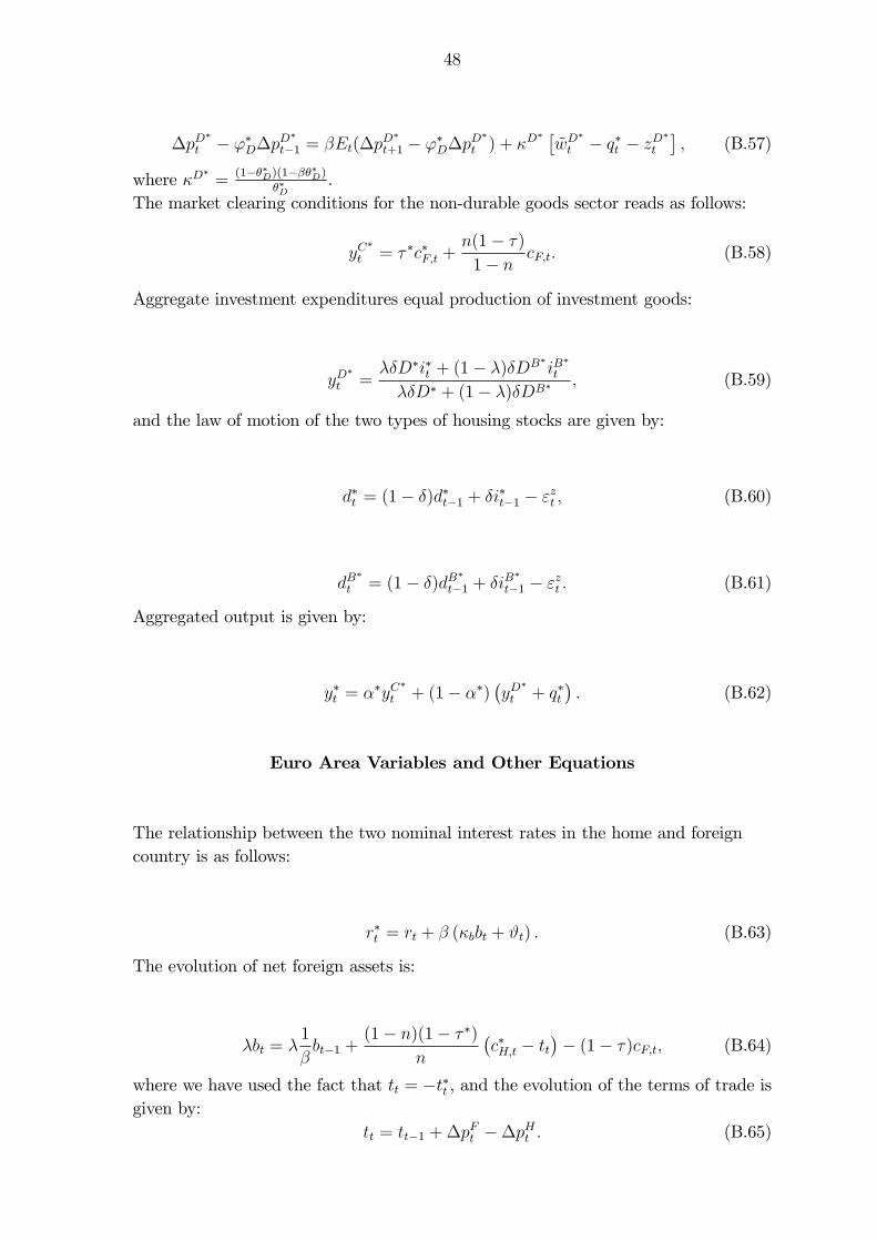
48

�pD�

t � '�D�pD�

t�1 = �Et(�pD�

t+1 � '�D�pD�

t ) + �D� �~wD

�

t � q�t � zD�

t

�; (B.57)

where �D�=

(1���D)(1����D)��D

.The market clearing conditions for the non-durable goods sector reads as follows:

yC�

t = � �c�F;t +n(1� �)

1� ncF;t: (B.58)

Aggregate investment expenditures equal production of investment goods:

yD�

t =��D�i�t + (1� �)�DB�iB

�t

��D� + (1� �)�DB�; (B.59)

and the law of motion of the two types of housing stocks are given by:

d�t = (1� �)d�t�1 + �i�t�1 � "zt ; (B.60)

dB�

t = (1� �)dB�

t�1 + �iB�

t�1 � "zt : (B.61)

Aggregated output is given by:

y�t = ��yC�

t + (1� ��)�yD

�

t + q�t�: (B.62)

Euro Area Variables and Other Equations

The relationship between the two nominal interest rates in the home and foreigncountry is as follows:

r�t = rt + � (�bbt + #t) : (B.63)

The evolution of net foreign assets is:

�bt = �1

�bt�1 +

(1� n)(1� � �)

n

�c�H;t � tt

�� (1� �)cF;t; (B.64)

where we have used the fact that tt = �t�t , and the evolution of the terms of trade isgiven by:

tt = tt�1 +�pFt ��pHt : (B.65)

49

The monetary policy Taylor rule conducted by the ECB reads:

rt = Rrt�1 + (1� R)� ��p

EMUt + �

�yEMUt � yEMU

t�1 + "zt��+ "mt ; (B.66)

where the euro area CPI and output is given by:

�pEMUt = n�pCt + (1� n)�pC

�

t ; (B.67)

yEMUt = nyt + (1� n)y�t : (B.68)

Finally, in Sections 4, when we include the macroprudential tools, we assume thatthey are linear functions of an indicator variable (�t and ��t ) which is either creditgrowth or credit to GDP in each country:

�t = ��t; (B.69)

��t = ���t : (B.70)

Shock Processes

All shocks included in the model evolve according to:

�Ct = ��;H�Ct�1 + "�;Ct ; (B.71)

�C�

t = ��;H�C�

t�1 + "�;C�

t ; (B.72)

�Dt = ��;D�Dt�1 + "�;Dt + "�;D;COMt ; (B.73)

�D�

t = ��;D�D�

t�1 + "�;D�

t + "�;D;COMt ; (B.74)

zCt = �Z;CzCt�1 + "Z;Ct + "Z;C;COMt ; (B.75)

zC�

t = �Z;CzC�

t�1 + "Z;C�

t + "Z;C;COMt ; (B.76)

zDt = �Z;DzDt�1 + "Z;Dt ; (B.77)

zD�

t = �Z;DzD�

t�1 + "Z;D�

t ; (B.78)

�!;t = (1� ��!) ��! + ��!�!;t�1 + u!;t; (B.79)

��!;t = (1� ��!) ��! + ��!��!;t�1 + u�!;t; (B.80)

#t = �##t�1 + "#t ; (B.81)

while the non-stationary innovation to the union-wide technology shock and themonetary policy shock are iid: "Zt and "

mt .

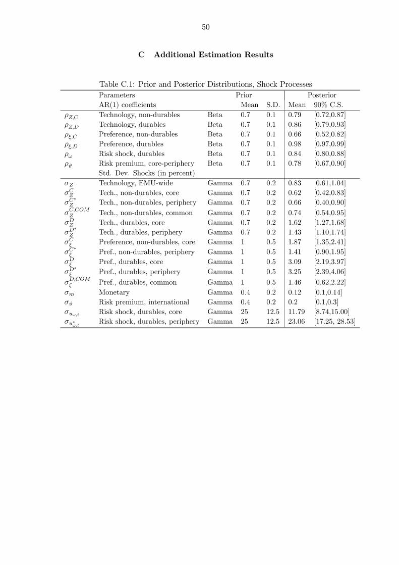
50

C Additional Estimation Results

Table C.1: Prior and Posterior Distributions, Shock ProcessesParameters Prior PosteriorAR(1) coe¢ cients Mean S.D. Mean 90% C.S.

�Z;C Technology, non-durables Beta 0.7 0.1 0.79 [0.72,0.87]�Z;D Technology, durables Beta 0.7 0.1 0.86 [0.79,0.93]��;C Preference, non-durables Beta 0.7 0.1 0.66 [0.52,0.82]��;D Preference, durables Beta 0.7 0.1 0.98 [0.97,0.99]�! Risk shock, durables Beta 0.7 0.1 0.84 [0.80,0.88]�# Risk premium, core-periphery Beta 0.7 0.1 0.78 [0.67,0.90]

Std. Dev. Shocks (in percent)�Z Technology, EMU-wide Gamma 0.7 0.2 0.83 [0.61,1.04]�CZ Tech., non-durables, core Gamma 0.7 0.2 0.62 [0.42,0.83]�C

�Z Tech., non-durables, periphery Gamma 0.7 0.2 0.66 [0.40,0.90]�C;COMZ Tech., non-durables, common Gamma 0.7 0.2 0.74 [0.54,0.95]�DZ Tech., durables, core Gamma 0.7 0.2 1.62 [1.27,1.68]�D

�Z Tech., durables, periphery Gamma 0.7 0.2 1.43 [1.10,1.74]�C� Preference, non-durables, core Gamma 1 0.5 1.87 [1.35,2.41]�C

�� Pref., non-durables, periphery Gamma 1 0.5 1.41 [0.90,1.95]�D� Pref., durables, core Gamma 1 0.5 3.09 [2.19,3.97]�D

�� Pref., durables, periphery Gamma 1 0.5 3.25 [2.39,4.06]

�D;COM� Pref., durables, common Gamma 1 0.5 1.46 [0.62,2.22]�m Monetary Gamma 0.4 0.2 0.12 [0.1,0.14]�# Risk premium, international Gamma 0.4 0.2 0.2 [0.1,0.3]�u!;t Risk shock, durables, core Gamma 25 12.5 11.79 [8.74,15.00]�u�!;t Risk shock, durables, periphery Gamma 25 12.5 23.06 [17.25, 28.53]

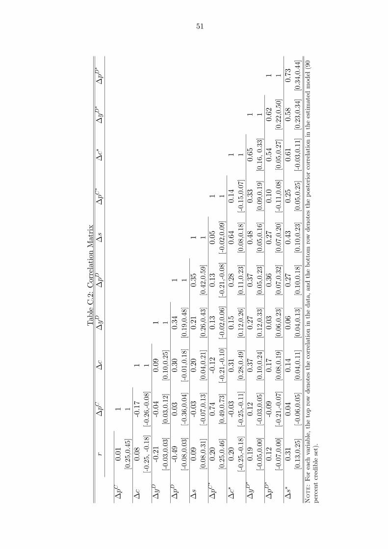
51

TableC.2:CorrelationMatrix

r�pC

�c

�yD

�pD

�s

�pC

��c�

�yD�

�pD

�

�pC

0.01

1[0.25,0.45]

1�c

0.08

-0.17

1[-0.25,-0.18]

[-0.26,-0.08]

1�yD

-0.21

-0.04

0.09

1[-0.03,0.03]

[0.03,0.12]

[0.10,0.25]

1�pD

-0.49

0.03

0.30

0.34

1[-0.08,0.03]

[-0.36,0.04]

[-0.01,0.18]

[0.19,0.48]

1�s

0.09

-0.03

0.20

0.21

0.35

1[0.08,0.31]

[-0.07,0.13]

[0.04,0.21]

[0.26,0.43]

[0.42,0.59]

1�pC

�0.20

0.74

-0.12

0.13

0.13

0.05

1[0.25,0.46]

[0.49,0.73]

[-0.21,-0.10][-0.02,0.06]

[-0.21,-0.08][-0.02,0.09]

1�c�

0.20

-0.03

0.31

0.15

0.28

0.64

0.14

1[-0.25,-0.18]

[-0.25,-0.11]

[0.28,0.49]

[0.12,0.26]

[0.11,0.23]

[0.08,0.18]

[-0.15,0.07]

1�yD�

0.19

0.12

0.37

0.27

0.37

0.48

0.33

0.65

1[-0.05,0.00]

[-0.03,0.05]

[0.10,0.24]

[0.12,0.33]

[0.05,0.23]

[0.05,0.16]

[0.09,0.19]

[0.16,0.33]

1�pD

�0.12

-0.09

0.17

0.03

0.36

0.27

0.10

0.54

0.62

1[-0.07,0.00]

[-0.21,-0.07]

[0.08,0.19]

[0.06,0.23]

[0.07,0.32]

[0.07,0.20]

[-0.11,0.08]

[0.05,0.27]

[0.22,0.50]

1�s�

0.31

0.04

0.14

0.06

0.27

0.43

0.25

0.61

0.58

0.73

[0.13,0.25]

[-0.06,0.05]

[0.04,0.11]

[0.04,0.13]

[0.10,0.18]

[0.10,0.23]

[0.05,0.25]

[-0.03,0.11]

[0.23,0.34][0.34,0.44]

Note:Foreachvariable,thetoprowdenotesthecorrelationinthedata,andthebottomrowdenotestheposteriorcorrelationintheestimatedmodel(90

percentcredibleset).

52

Table C.3: Posterior Variance Decomposition (90 percent con�dence set)Shocks

r Common Nondurable Technology Core Nondurable Technology[31.9, 60.2] [8.3, 27.3]

�pC Common Nondurable Technology Core Nondurable Technology[25.5, 51.1] [15.5, 40.9]

�c Core Nondurable Preference EMU-wide Technology[48.5, 71.6] [15.5, 36.7]

�yD Core Durable Preference Core Durable Technology[31.2, 60.3] [19.5, 40.0]

�pD Core Durable Preference Core Durable Technology[30.4, 54.7] [16.8, 29.5]

�s Risk Core Core Durable Preference[34.9, 59.8] [17.2, 41.7]

�pC�Common Nondurable Technology Country Risk Premium

[19.2, 39.6] [13.8, 36.8]�c� Periphery Nondurable Preference EMU-wide Technology

[23.1, 56.7] [21.0, 49.0]�yD

�Periphery Durable Preference Periphery Durable Technology

[34.3, 58.2] [19.4, 33.3]�pD

�Periphery Durable Preference Periphery Durable Technology

[31.5, 61.2] [13.4, 33.1]�s� Risk Periphery Periphery Durable Preference

[62.3, 81.8] [8.9, 19.6]

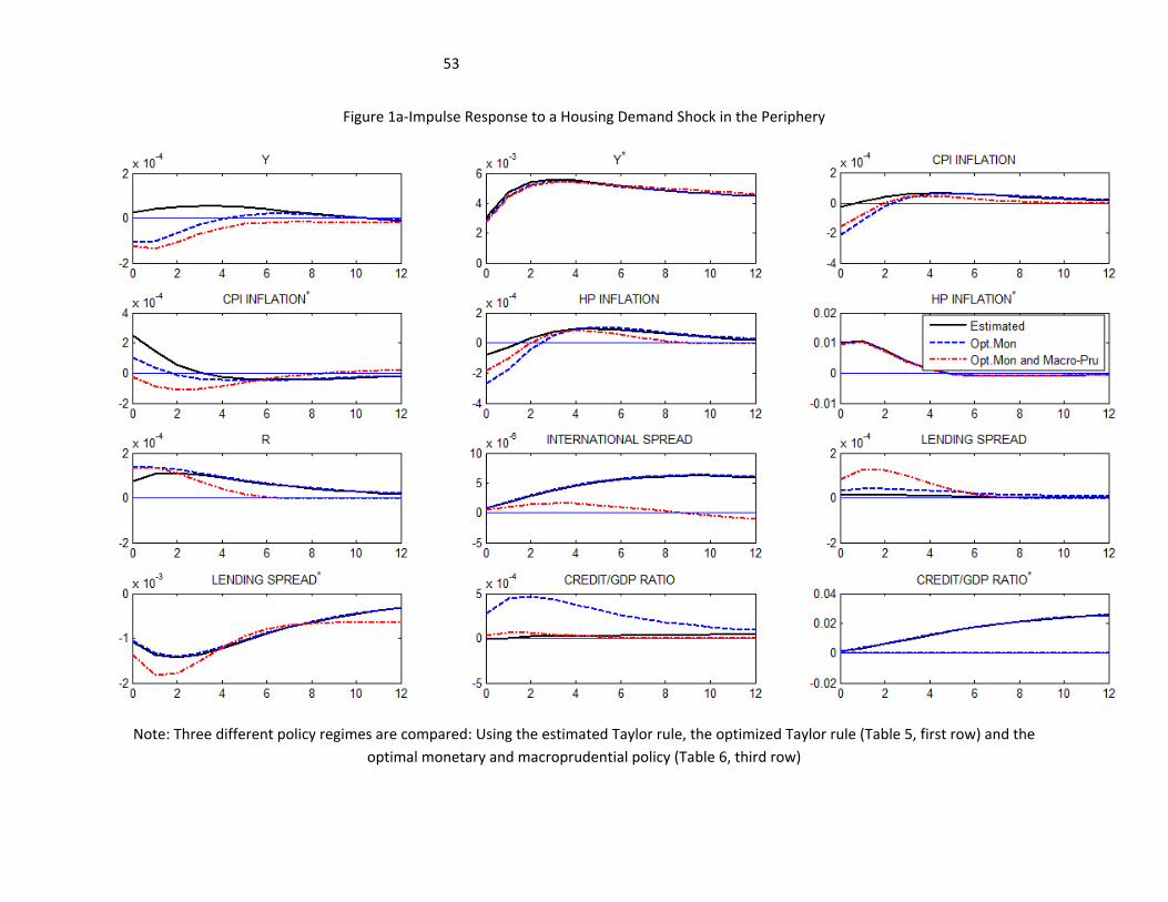
  53

Figure 1a-Impulse Response to a Housing Demand Shock in the Periphery

Note: Three different policy regimes are compared: Using the estimated Taylor rule, the optimized Taylor rule (Table 5, first row) and the optimal monetary and macroprudential policy (Table 6, third row)

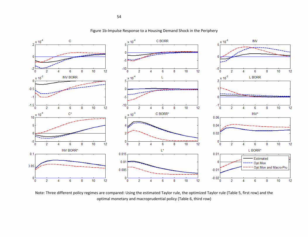
54

Figure 1b-Impulse Response to a Housing Demand Shock in the Periphery

Note: Three different policy regimes are compared: Using the estimated Taylor rule, the optimized Taylor rule (Table 5, first row) and the optimal monetary and macroprudential policy (Table 6, third row)

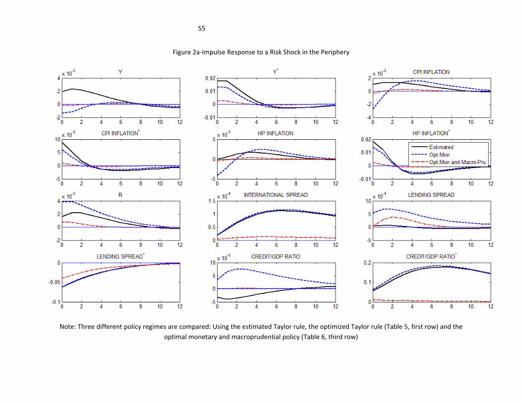
55

Figure 2a-Impulse Response to a Risk Shock in the Periphery

Note: Three different policy regimes are compared: Using the estimated Taylor rule, the optimized Taylor rule (Table 5, first row) and the optimal monetary and macroprudential policy (Table 6, third row)

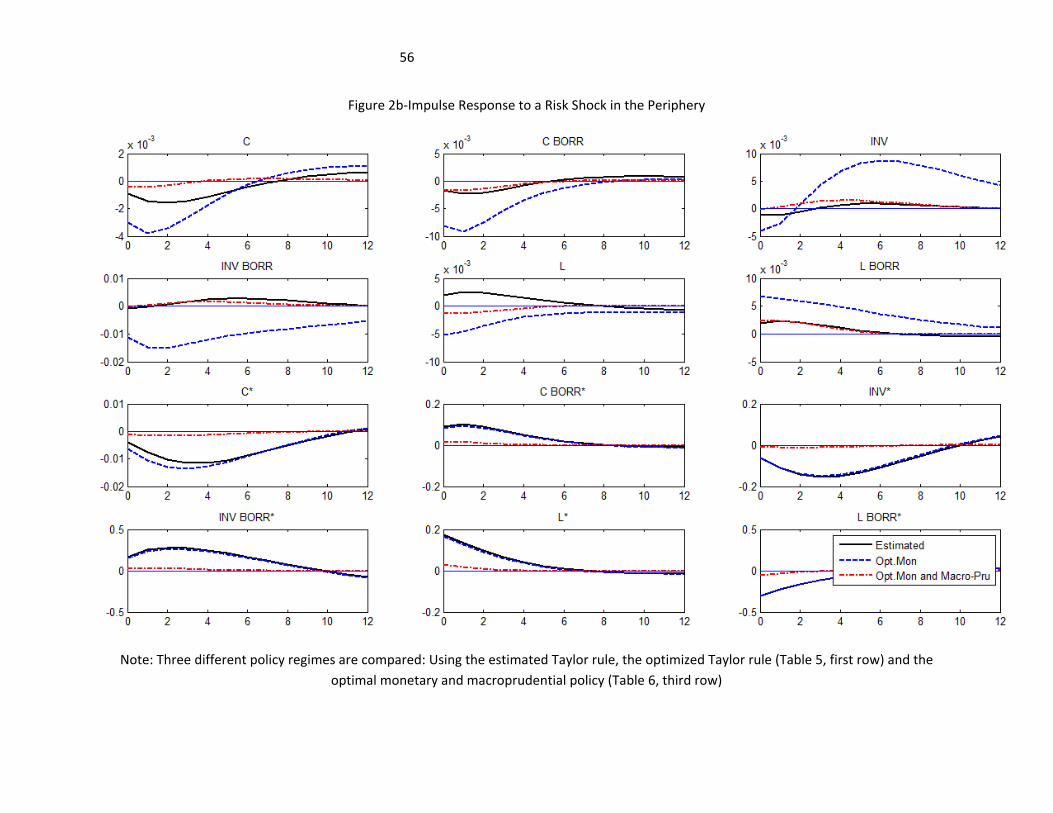
56

Figure 2b-Impulse Response to a Risk Shock in the Periphery

Note: Three different policy regimes are compared: Using the estimated Taylor rule, the optimized Taylor rule (Table 5, first row) and the optimal monetary and macroprudential policy (Table 6, third row)

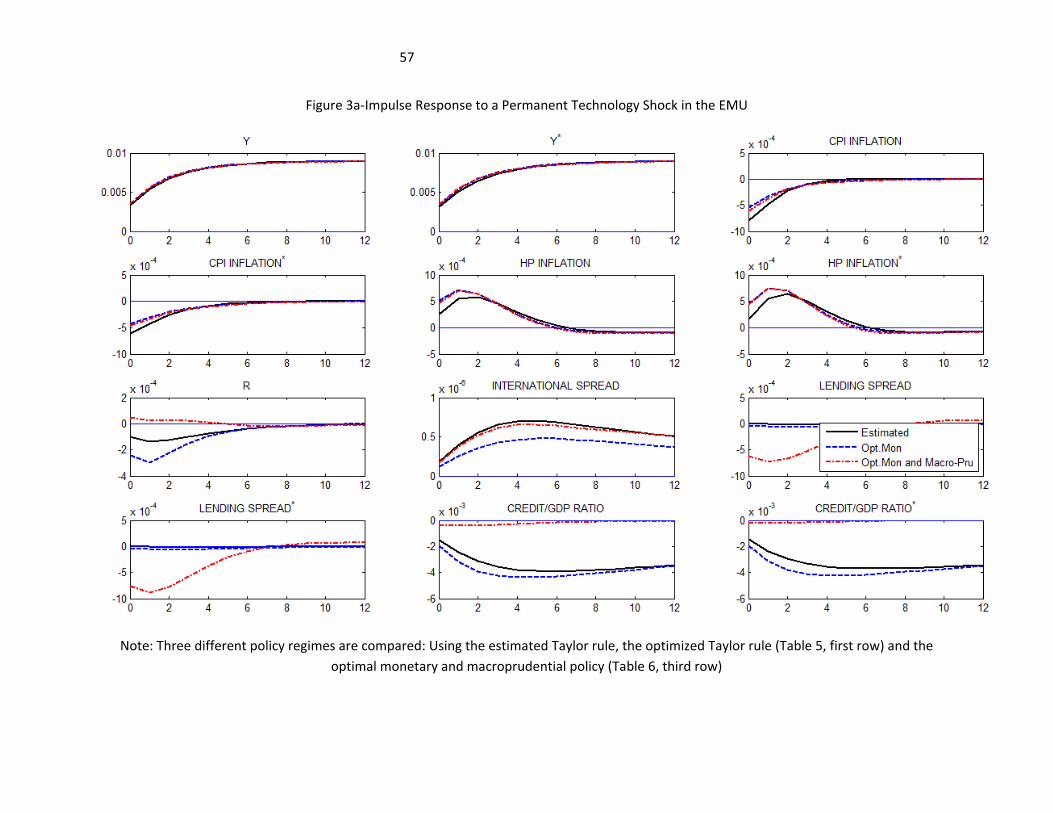
57

Figure 3a-Impulse Response to a Permanent Technology Shock in the EMU

Note: Three different policy regimes are compared: Using the estimated Taylor rule, the optimized Taylor rule (Table 5, first row) and the optimal monetary and macroprudential policy (Table 6, third row)

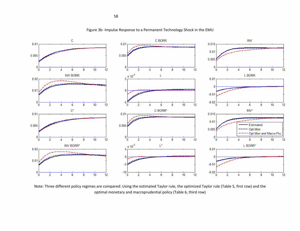
58

Figure 3b- Impulse Response to a Permanent Technology Shock in the EMU

Note: Three different policy regimes are compared: Using the estimated Taylor rule, the optimized Taylor rule (Table 5, first row) and the optimal monetary and macroprudential policy (Table 6, third row)

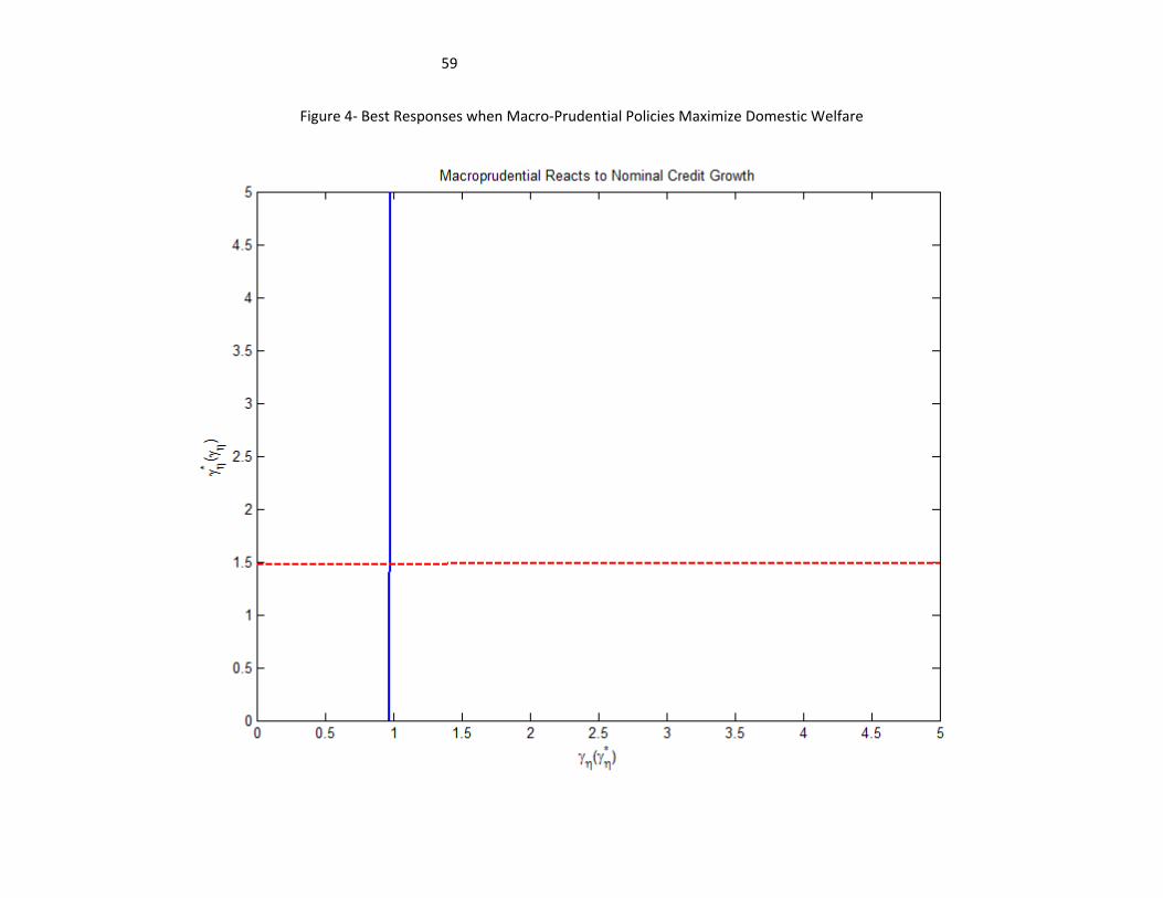
59

Figure 4- Best Responses when Macro-Prudential Policies Maximize Domestic Welfare