Embed Size (px)
Citation preview
ELSEVIER Journal of Computational and Applied Mathematics 86 (1997) 3-16
JOURNAL OF COMPUTATIONAL AND APPLIED MATHEMATICS
Moment matching method for numerical solution of MTL equations in interconnect analysis 1
Zhaojun BaP'*, Antonio Orlandi u, William T. Smith c a Department of Mathematics, University of Kentucky, Lexington, KY 40506, USA
b Department of Electrical Engineering, University of L'Aquila, 67040 Poggio di Roio, L'Aquila, Italy c Department of Electrical Engineerin 9, University of Kentucky, Lexington, KY 40506, USA
Received 7 January 1997; received in revised form 5 June 1997
Dedicated to William B. Gragg on the occasion of his 60th birthday
Abstract
Multiconductor transmission line (MTL) analysis is a popular technique for evaluating high-speed electrical intercon- nects. Typically, MTLs are modeled in the Laplace domain and similarity transformations are used to decouple the MTL equations. For high-speed systems, however, direct solution of the MTL equations at a large number of frequencies is computationally very expensive. Recent studies have employed moment matching techniques to approximate the solution for the MTL equations and improve the computational efficiency. In this study, a generalization of the method of char- acteristics is further studied for solving the MTL equations for lossy transmission lines. An efficient recursive solution for generating the moments of eigenvalues and eigenvectors is presented. Numerical results of this moment matching technique agree with the direct solution methods up to 10GHz.
Keywords." Multiconductor transmission line (MTL) equations; Moment matching technique; Interconnect analysis; Eigen- value decomposition
AMS classification." 65C20; 65F15; 65L05
I. Introduction
The electronics industry has entered an age where electrical interconnects between components present the most significant limitations on the overall performance of a high-speed digital system.
* Corresponding author. 1 Numerical simulations were carried out at High-Performance Computing Laboratory of College of Arts and Sciences
(CAS), University of Kentucky (UK). The Laboratory is funded in part by a grant from NSF and CAS and Research and Graduate Studies at UK.
0377-0427/97/$17.00 © 1997 Elsevier Science B.V. All rights reserved PH S 0 3 7 7 - 0 4 2 7 ( 9 7 ) 0 0 1 4 5 - 3
4 Z. Bai et al./Journal of Computational and Applied Mathematics 86 (1997) 3-16
It is, therefore, imperative that the signal propagation on these interconnects be accurately modeled in a design simulation. Multiconductor transmission line (MTL) theory is a very popular method for analyzing interconnect cables and data buses. In order to accurately represent the interconnects, the transmission lines must be modeled as lossy conductors. The solution for the lossy MTL equations is straightforward if solved in the frequency domain for a single frequency. Typically, the MTLs are modeled in the Laplace domain and a similarity transformation is used to decouple the equations at the desired frequency. However, the power spectrum of these digital signals is very wideband due to high clock speeds and very short-time transients and, hence, single-frequency analysis is inadequate. One approach to evaluating the equations over a broad range of frequencies is to perform similarity transformations for a near continuum of frequencies using the single-frequency technique. This is computationally inefficient as eigendecompositions must be performed for each frequency.
The problem encountered in the eigendecomposition for lossy multiconductor transmission lines is that the transformation matrices used to diagonalize the system matrices are functions of the complex frequency s. For an arbitrary number of transmission lines, it is not feasible to determine the exact analytical expressions for the frequency-dependent eigensolution. An approximate series solution for the eigendecomposition was proposed by Bracken et al. [3] using a generalization of the method of characteristics [4]. The eigenvalue and eigenvector matrices are expanded as functions of s and a moment matching technique using recursion was proposed for determining an approximate series so- lution for the eigendecomposition. It is the recursive solution technique that is the focus of this paper.
The rest of this paper is organized as follows. In Section 2, the MTL equations used to characterize the voltages and currents on a transmission line are presented in the time and frequency domains. It is more straightforward to obtain the solution of these MTL equations in the Laplace domain. Various methods for the numerical solution of the MTL equations are reviewed. In Section 3, we discuss the structure of the eigendecomposition of the transformation matrix M(s) for the MTL equations in frequency domain. The existence of the power-series expansions of the eigenvalues and eigenvectors of M(s) and numerical computation of the coefficients of the series are presented. The numerical solution of the MTL equations by the moment expansion method of the eigendecomposition of M(s) is presented in Section 4. Issues on the convergence radius and rate of moment expansion of the eigendecomposition of M(s) are addressed there. Numerical results for solving MTL equations of interconnect models are in Section 5. Concluding remarks are in Section 6.
2. MTL equations and frequency-domain analysis
The MTL equations are the governing equations for n-uniform lossy coupled transmission lines:
~---~v(x, t) + Ri(x, t) ÷ L-~i(x, t) = O, ( 1 )
--~xi(X,t) + Gv(x,t) + C v(x,t) = 0, (Z)
where v(x,t) and fix, t) are the vectors of line voltages and line currents, O<~x<~d, f the length of transmission line, and t the time variable. L, C, R and G are the inductance, capacitance, resistance and conductance matrices, respectively. All of these matrices are n x n and symmetric. Further, we also require that the conductance matrix G be nonsingular. In the majority of applications, the
z. Bai et al./Journal of Computational and Applied Mathematics 86 (1997) 3-16 5
voltages v(x,t) and currents i(x,t) are of most interest at the inputs (v(O,t), i(O,t)) and outputs (v(f , t) , i(~,t)) of the transmission lines. In that regard, the solutions of (1) and (2) provide the relationship between the voltages at the input and output. In order to uniquely solve these equations, (1) and (2) are augmented with equations describing the initial conditions.
The MTL equations (1) and (2) can be decoupled into the second-order partial differential equations:
(~2 ~2 Cq ~xiV(X, t )= LC-~sv(x, t) + (RC + LG)-~v(x, t) + RGv(x, t), (3)
0 2 0 2 8 ~xxii(x, t) = CL-~i(x , t) + (CR + GL)-~i(x, t) + GRi(x, t). (4)
These are also called the generalized wave equations. In general, there are no closed-form (explicit) solutions for these equations [7, 10].
Taking the Laplace transform of (1) and (2) produces a linear homogeneous system of 2n equations
0 -~xV(X,S) = - ( R + sL)i(x,s), (5)
0 -~xi(X, s) = - ( G + sC)v(x, s), (6)
where s is a frequency parameter. Define the transformation matrix
[ 0 M(s) = G + sC
then (5) and (6) can be written in the compact matrix form as
= [ v(x,,) ] r x,s l 0 -~x L i(x,s) j i(x,s) j"
By the standard theory of linear systems of ordinary differential equations [6], the solution of (7) is of the form
i(x,s) J L i(O,s) j ' (8)
where v(O,s) and i(O,s) are initial conditions. The matrix e -xM(*) is called a fundamental matrix of the system or chain parameter matrix in the interconnect analysis [11]. The initial values v(0,s) and frO, s) are determined through additional equations that incorporate the terminal conditions in the electrical network.
If the transformation matrix M(s) is diagonalizable and M(s) = T- l (s )A(s)T(s) is an eigende- composition of M(s), then the solution of (7) can be written as
i(x,s) J --r-l(s)e-xA(*)T(s) (9) L i(O,s) j"
A number of numerical approaches for solving Eqs. (5) and (6) are discussed in [11, 5]. There are essentially two classes of methods. The first class of methods explicitly computes the chain parameter
6 z. Bai et al./Journal of Computational and Applied Mathematics 86 (1997) 3 16
matrix e -xM(~) or the eigendecomposition of the transformation matrix M ( s ) at each frequency point s. We refer to that as a direct method. The direct method is a general technique. High-quality sot~ecare for computing the matrix exponential and eigendecomposition are widely available; e.g. the public- domain software package LAPACK [1]. However, this class of methods can be very time consuming if the number of transmission lines are large and the responses at a large number of frequencies are desired. It requires an order of n 3 operations to compute either the matrix exponential or the eigendecomposition. The total cost will be on the order of kn 3, where k is the number of the frequencies.
The second class of methods is based on the asymptotic waveform evaluation (AWE) technique. AWE is a moment matching technique first used in the analysis of linear circuit systems [12]. Namely, one expands the chain parameter matrix e -xM(s) [5] or the eigendecomposition of M ( s ) [3] in the power series of the frequency parameter s. The coefficients of the power series are called the moments of the system. Once these coefficients are computed, the computation of the chain parameter matrix e -xM(s) or the eigendecomposition of M ( s ) only costs an order of n 2 operations at each frequency. The total cost of this class of methods is, in general, on the order of n 3 q- kn 2, where k is the number of the frequencies. Therefore, the AWE-based technique is an attractive way to solve the MTL equations and can be significantly more efficient than the direct method. However, because of power-series expansions and approximations, the central problems become how to efficiently compute the coefficients and accurately determine the convergence radius and rate of the series expansions.
In this paper, we will further study the moment matching method for computing the eigendecom- position of the transformation matrix M ( s ) , which is first presented in the work of Bracken et al. [3]. We will first discuss the structure of the eigendecomposition of M ( s ) , and then propose an efficient method to compute the coefficients in the power-series expansion of the eigenvalue and eigenvector matrices of M(s ) . Numerical examples will be presented to demonstrate the accuracy and limitations of this approach.
To end this section, we note that the linear system (5) and (6) could be decoupled into second- order systems:
t? 2 Os 2 v(x ,s) = (R + sL ) (G + sC)v(x , s ) ,
~2 Os 2 i(x, s) = (G + sC) (R + sL)i(x, s),
which have solutions of the forms
v(x, s) = v(O, s)e --~(~)~,
i(x, s) = i(O, s)e +'xs)x,
where 7(s) is the complex propagation mode constant. Substituting the solution form into the wave equations yields the matrix eigenvalue problems,
[(R + sL) (G + sC) - 72(s)I]v(O,s) = O,
[(G + s C ) ( R + sL) - 72(s)I]i(O,s) = O.
Z. Bai et al./Journal of Computational and Applied Mathematics 86 (1997) 3-16 7
A similar moment expansion method can also be developed for this second-order system. But, since, we can efficiently solve the original first-order system, it is less desirable to solve the second-order system. In particular, if there is a significant delay between the input aad output signals, the solutions of second-order equations may suffer in accuracy [3].
3. Power-series expansion of eigendecomposition of transformation matrix M(s)
To efficiently compute the power-series expansion of the eigenvalues and eigenvectors of the transformation matrix M(s), let us first study the structure of the eigenvalues and eigenvectors. We first note that M2(s) is a block diagonal matrix,
M2(s)= I (R + sL)(G + sC ) 0 1 0 (G ÷ sC)(R ÷ sL) "
It can be shown that the matrices (R + sL)(G + sC) and (G + sC)(R + sL) have the same eigenvalues and, furthermore, if at least one of the matrix G+sC or R+sL is nonsingular, then (R+sL)(G+sC) and (G + sC)(R + sL) are similar. Let
A(s)(R + sL)(G ÷ sC)A-l(s) = FZ(s)
be the eigendecomposition of (R + sL)(G + sC), where AH(s) is the left eigenvector matrix and FZ(s) is the corresponding eigenvalue matrix. Here it is assumed that the matrix (R + sL)(G + sC) is diagonalizable, say all eigenvalues of (R + sL)(G + sC) are distinct. Then it is straightforward to verify that if G + sC is nonsingular, then
B(s) = - r ( s ) A ( s ) ( G + sO) -1
gives the eigendecomposition of (G + sC)(R + sL)
B(s)(G + sC)(R ÷ sL)B-l(s) = F2(s).
By some algebraic manipulation, one immediately shows that the eigendecomposition of the trans- formation matrix M(s) poses the following structure:
M(s) = T-l(s)A(s)T(s), (lO)
where
1 0 l [ A ( s ) - B ( s ) J and A ( s ) = F(s)
The structural eigendecomposition (10) of M(s) reveals that although M(s) is a 2n × 2n matrix, its eigenvector matrix is formed by two n × n matrices A(s) and B(s). Furthermore, the eigenvalues of M(s) appear in pairs of ±2. In the following, we will exploit this fact for computing the power-series expansion of eigenvalues and eigenvectors of M(s) and solving the MTL equations (5) and (6).
8 Z. Bai et al./Journal of Computational and Applied Mathematics 86 (1997) 3-16
Note that the inverse of T(s) is given by
[A(s) B(s) ]-1 1 [A-I(s) A-I(s) ] T-I(s) =
LA(s) -a(s)J = 2 [B-I(s) --a-m(3')J
and furthermore, the columns of T-I(s) are the right eigenvectors of the transformation matrix M(s). It needs to be determined whether the eigenvalues and eigenvectors of M(s) can be expressed
as power series in s. In other words, determine whether they are holomorphic (regular analytic) functions of s in the neighborhood of s = 0. We may write M(s) as
o ~]+~[o oJ. M(s) = [ a
i.e., M(s) may be viewed as the perturbed matrix of
[0o :1 By linear operator perturbation theory [9], we know that if this matrix has distinct eigenvalues, then the eigenvalues and eigenvectors of M(s) are the analytic functions for sufficiently small Isl. Specifically, the eigenvalue matrix A(s) and the eigenvector matrix T(s) of the transformation matrix M(s) can be written in power-series forms in the neighborhood of s = 0:
01 [: 0] 0] 0 F0 + s F1 +s2 0 F2 + " " (11)
and
[Ao I LAa ~--- -4-S -~-S 2 + ' ' ' . -do -Bo A1 -BI A2 -B2
(12)
The coefficients of s k are called the kth moments of the eigenvalues or eigenvectors, respectively. In most studies of the perturbation of linear operators, one is only interested to find the coefficients of the first (s) and second (s 2) terms of the series [9]. However, because s may not be small, in general, we are interested to compute an arbitrary number of the coefficients (moments) A;, Bi and/7,.
From the eigendecomposition (10) of M(s) and the power-series expansions (11) and (12) of A(s) and T(s), the coefficients of the s°-terms give the equation
[~i ~o [0o :] [: 01° [:0 ° ] =0 . (13)
This is just an eigendecomposition of M(s) at s = 0.
Z. Bai et al./Journal of Computational and Applied Mathematics 86 (1997) 3-16
Equating the coefficients of the sl-terms in the eigendecomposition (10) yields
_BII [0 R] _ [-~ ~o] [~: BI -BI ]
o][ o ,o][o 0 F1 Ao -Bo Ao -Bo
In general, equating the coefficients of the sk-terms, one can find the following equation for the coefficients Ak, Bk and Fk for any k ~> 1:
[oo :1_ o0 0 ~ Ao -Bo [Ak-I --Bk-l] C
+~i=~ 0 ~ [Ak-i --Bk_i "
By further algebraic simplification, one can show that Eqs. (13) and (14) can be reduced to
AoR + FoBo = 0, (15)
BoG + FoAo = 0 (16)
and
AkR + FoBk + FkBo = Ek-1, (17)
BkG + FoAk + FkAo =Fk-1 (18)
for k t> 1, where
k - I k - 1
Ek-1 : - A k _ l L - y ~ I~iBk-i and Fk-l = - B k _ I C - ~ FiAk-i. i=l i=l
We now derive a method to solve Eqs. (15)-(18) for Fk, A~ and Bk for k=0 , 1,2,.... First, when k = 0, let
Ao(RG)Ao 1 = lo 2
be the eigendecomposition of RG and let
Bo = - FoAo G -1.
It can be immediately recognized that Ao, Bo and Fo satisfy Eqs. (15) and (16) simuRaneously. Note that Bo is also the left-eigenvector matrix of GR, namely Bo(GR)Bo 1 = i-ol.
10 Z. Bai et al./Journal of Computational and Applied Mathematics 86 (1997) 3-16
For any k~>l, by multiplying the matrix Bo 1 on the right-hand side of (17) and the matrix Ao 1 on the right-hand side of (18) and using Eqs. (15) and (16), we obtain
- A k A o l Fo + FoBkBo 1 + Fk = Ek_lBo 1, (19)
- B k B o l Fo 4- FoAkAo 1 -~ Fk = F k _ I A o 1. (20)
Subtracting Eq. (19) from (20) yields
XkFo + FoXk = Fk_lAo 1 - E k _ l B o 1, (21)
where Ark is an auxiliary matrix defined as
Xk = AkAo 1 - BkBo 1.
Eq. (21) is a well-known Sylvester matrix equation with unknown Ark [8]. Since F0 is a diagonal matrix, the solution Xk is immediately given by
1 (Xk )ij -- ~i ~ - ~ (Fk-lA°l - - g k - l B ° l )ij
for i , j = 1 ,2 , . . . ,n , where 7i are the diagonal entries of F0, F0 = diag(7i) and (Z)ij denote the ( i , j ) elements of a matrix Z.
On the other hand, adding Eq. (19) to (20) yields
--Ykl'o q- FoYk -q- 2Fk = Fk_lAo 1 + gk_lBo 1 ,
where Yk is the second auxiliary matrix and defined as
Yk = AkAo 1 + BkBo 1.
Note that the diagonal entries of -YkFo+FoYk are all zeros and that the desired matrix Fk is diagonal. We know have
Fk = ½diag(F~_lAo 1 + Ek_IB o' ),
where diag(Z) denotes the diagonal matrix with diagonal entries of a matrix Z. Furthermore, the off-diagonal entries ( i , j ) of the matrix Yk are determined by
1 ( gk )ij -- - - ( F k - l A o 1 -~- Ek- ,Bol )ij
~j -- ~2 i
for i , j = 1,2 . . . . ,n and i # j . Hence, the diagonals of Yk can arbitrarily be chosen. After determining the auxiliary matrices Xk and Yk, the desired coefficient matrices Ak and Bk are
given by
A~ + Xk)Ao, =½(Y
Bk = ½(Yk - Xk)Bo.
Z. Bai et al./ Journal of Computational and Applied Mathematics 86 (1997) 3-16 11
In summary, we have the following algorithm for computing the coefficient matrices Fk, Ak and Bk of the first m + 1 terms in the power series expansion of the eigenvalue and eigenvector matrices A(s) and T(s) for the transformation matrix M(s):
M o m e n t - G e n e r a t i n g A l g o r i t h m - - compute the eigendecomposition of RG: Ao(RG)Ao 1 = F02, F0 = diag(7~), - - Bo =-FoAoG -1, - - for k = 1 ,2 , . . . ,m
• ek_l = - A k _ , L - 5B -j,
• Fk-1 = - B k _ l C - E~Z 1 FjAk_j, • Ek-i :=Ek-lBo l, • Fk_ 1 :~---Fk_lAo 1, • Xk = F k - 1 - Ek-1, • (Xk)~j:=(Xk)~j/(y~ +Tj) for i , j = 1,2, . . . ,n , • Yk =Fk_l + E k - 1 , • F~ = ½diag(Yk), • set the diagonal entries of Yk to be zero, • (Yk)ij:=(Yk)ij/(Tj- 7i); for i , j : 1,2, . . . ,n , i C j , • Ak +Xk)Ao,
• Bk = ½(Yk -- X,~)Bo, - - end
The initial cost for computing the eigendecomposition of RG is about 25n 3 ÷ O(n 2) [8]. In the loop of k, the cost of computing one set of coefficients F~,Ak and Bk is 12n 3 + 2kn 2 ÷ O(n 2) flops. In summary, the total cost of computing the first m ÷ 1 terms of the power-series expansion of the eigenvalue and eigenvector matrices of M(s) is (30 + 12m)n 3 + m(m + 1)n 2 + O(n 2) flops.
The above discussion can be generalized to the power-series expansion of the eigenvalue and eigenvector matrices of M(s) about any given frequency So # 0 and c¢, namely the Laurent expansion. In principle, to expand M(s) at any given point So, it can be re-written as
[ 0 [0 L 1 M ( s ) = G+soC 0 + ( S - S o ) C 0 '
i.e., M(s) can be viewed as the perturbed matrix of
I 0 R ÷ soL 1" G ÷ soC 0
With the assumption that the eigenvalues of this unperturbed matrix are distinct, then the eigenvalues A(s) and eigenvectors T(s) of M(s) can be expanded as
A(s) = 0] E 10] 01 + (s - So) + (s - s0) 2 + . . . 0 F0 0 5 0 5
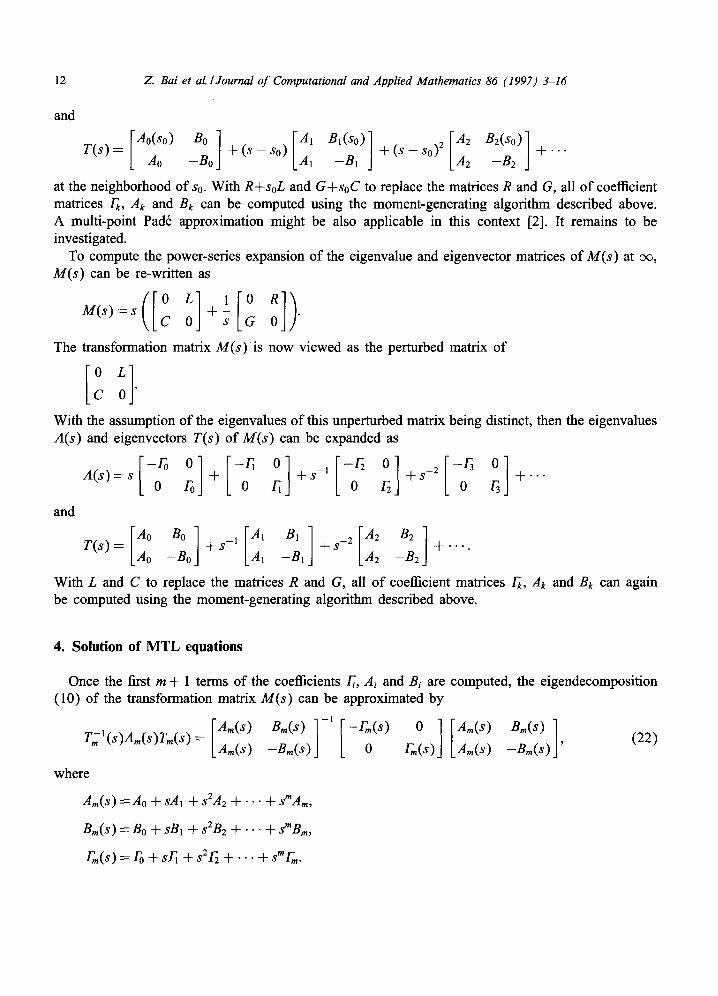
12 Z. Bai et al./Journal of Computational and Applied Mathematics 86 (1997) 3-16
and
= + (s - So) + (s - So)2 + . . . A0 -B0 A1 - B I A2 -B2 J
at the neighborhood of So. With R+soL and G+soC to replace the matrices R and G, all of coefficient matrices Fk, Ak and Bk can be computed using the moment-generating algorithm described above. A multi-point Pad6 approximation might be also applicable in this context [2]. It remains to be investigated.
To compute the power-series expansion of the eigenvalue and eigenvector matrices of M ( s ) at e¢, M ( s ) can be re-written as
- - °
s G 0
The transformation matrix M ( s ) is now viewed as the perturbed matrix of
With the assumption of the eigenvalues of this unperturbed matrix being distinct, then the eigenvalues A(s) and eigenvectors T(s) of M ( s ) can be expanded as
[: o I [: o] [_:o A ( s ) = s Fo + F1 + s - l F2
and
]+s2E 01 o r3 +
[ IB11 [A2 2] _]_S -1 _]_S -2 -q- . . . . Ao -Bo A1 -B1 .42 -B2
With L and C to replace the matrices R and G, all of coefficient matrices Fk, Ak and Bk can again be computed using the moment-generating algorithm described above.
4. Solution of MTL equations
Once the first m + 1 terms of the coefficients ~, Ai and B; are computed, the eigendecomposition (10) of the transformation matrix M ( s ) can be approximated by
T2l(s)Am(s)Tm(s) = "Am(s) Bin(s)
Am(s) -Bm(s)
where
Am(s) =,40 q- sA1 q- $2A2 + . . . + smAm,
-1 -r.(s) o ] [a.(s) o Vm(S) /Am(s)
BIn(S) = BO ~- sB1 -Jr- s2B2 + . . . + smBm,
B~(s) ] (22) -Bin(s) '
F,n(S) = Fo +sE +sEFz + . . - +StaG.
Z. Bai et al./Journal of Computational and Applied Mathematics 86 (1997) 3-16 13
For a given frequency s, the matrix polynomials Fro(s), Am(s) and Bin(s) c a n be efficiently evaluated with Homer's rule. For example, Am(s) can be evaluated as follows:
Horner's rule for matrix polynomial evaluation • W = A m , • f o r i = m - 1 down to 0;
- - W : = s W + Af; • end
On the return W = Am(s). The cost of computing Am(s) is only 2ran 2 floating point operations. Furthermore, with an additional order of n 2 operations, the rows of Tin(s) (i.e., the left approximate eigenvectors of M ( s ) ) can be normalized to have unit length.
With the approximate eigendecomposition (22) of the transformation matrix M(s) , using Eq. (9), approximate solutions of MTL equations in the frequency domain are given by
Om(X , S ) z - - ½Am l(S)[(e -xr'~s) + e xr.~s) )Am(s)v(O, s) + (e -xr'~s) - e xr'~) )B,,(s)i(O, s)]
and
im(X,S) = -½B~l(s )[ (e -xr~(s) - eXr~(s))Am(S)v(O,s) + (e -xr~(s) + eXr'(S))B,,(s)i(O,s)].
Note that since Fro(s) is a diagonal matrix, the matrix exponential e ~r'(s) is also a diagonal matrix, which can be computed directly. The total cost of solving the MTL equations in the frequency domain for k frequencies is about (36 + 12m)n 3 + 2kmn 2.
To determine an expansion point So and the required number of moments m to achieve the desired accuracy of the approximate eigendecomposition, one must know the radius and rate of the conver- gence of the power series expansion of the eigenvalues and eigenvectors A(s) and T(s) of M(s) . There is no known practical method to quantitatively determine the expansion point So and the number of the moments m. This remains an open problems for the moment matching method. For example, a study of convergence radii and error estimates of power series expansions of eigenvalues and eigen- vectors for a linear operator is presented in [9, p. 88]. However, the results are largely theoretical.
In practice, we can easily evaluate the backward accuracy of the approximate eigendecomposition (22) by computing the quantity
II Tm(s)M(s) - am(s)T,n(S)l I
IIM(s)[[llZm(s)ll ' ( 2 3 )
where the matrix norm can be chosen as the 1-norm or the c<)-norm, which can be computed with an order of n 2 operations. We propose to use this measure to heuristically determine whether we need to select a new expansion point So and increase the number of moments m. More discussion follows by examples in next section.
5. Numerical example
In this section, we present an example for a lossy 8-conductor multiconductor transmission line over a ground plane. Simulations were also carried out on 4-conductor and 40-conductor transmission lines. The results are similar to the ones presented here.
14 Z. Bai et al./Journal of Computational and Applied Mathematics 86 (1997) ~16
l o 0 . . . . . . . . , . . . . . . . . , . . . . . . . .
10 ~
lo-'
10 4 / ..- /
.." /
+."'"" "'+'" /' / / m =
. . . . • / +.-+ /
. . . " / / . . ' , - /
..." / / 24
m=4 .." m=8 I / // / ...... /. /I m=12 /
+..+ / /
. . . . . . . , i , , , , , , , , i . . . . . . . ,
10" 10 + 10 s 10 s 10 7 Frequency (Hz)
104
.! 10 -1o
10-+:
10 -1~
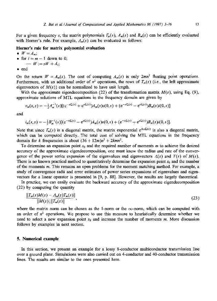
Fig. 1. Relative errors of vm(O.5, s) versus the number of moments m.
The ground plane of the lossy 8-conductor multiconductor transmission line provides the signal return path. The 8 x 8 inductance and capacitance matrices (L and C, respectively) were generated using a method of moments code [11]. The losses are characterized by the resistances and con- ductances defined in the R and G matrices, respectively. The line is Y = 0.5 m in length. The lines are terminated with 50 ~2 loads. The lines are excited with sources connected to the near end of lines 1 and 4 and the far ends of lines 5 and 6. These initial conditions v(O,s) and i(O,s) were determined using the chain parameter method [11]. It is augmented with equations describing the terminal conditions (sources, loads) to determine the initial values.
In this example, all entries of the inductance matrix L are of the orders 10-7-10 -9, capacitance matrix C entries are of the orders 10-t l -10 -14, resistance matrix R entries are of the order 10 and conductance matrix G entries are of the order 10-2-10 -3.
Fig. 1 plots the relative errors of Vm(O.5, S) versus the number of moments used to compute the eigendecomposition. The plot for the relative errors of im(O.5,S) is similar. The relative errors of Vm(O.5, S) and im(0.5,s) are measured by
[ [ / ) m ( 0 . 5 , S ) - - V o ( 0 - S , s ) I I and Ilim(0.5,S)-- ie(X,S)[I IlvoC0.5,s)ll II/eC0.5,s)ll '
where vc(0.5,s) and ie(0.5,S) are computed by the direct eigendecomposition method. The series expansions were performed about s = 0. From the figure, one can see that frequency range of acceptable error of the solution increases with the increasing of the number of moments m. In addition, we also see that when the number of moments are increased beyond m = 24, the frequency range does not continue to increase as the radius of convergence begins to limit the accuracy of the solution.
Z Bai et al./Journal of Computational and Applied Mathematics 86 (1997) 3-16 15
lO 0
lO 9
lO-'
1o"
elO 4 o ® -1( ._>m 10
10 -n
10 -14
10 -1~
lO-1'
10"
relative errors of eigendecomposi~ns and v_m(0.5,s) (m=l 2)
O ¢"
6 .xll
6 × ?! : X ii
0 ~ :: .. . . . : ×
/Y
i
X
., .:
i , i ,
i i
3 4
O" 0"" .XI
x !i .X" "
)4"
x' i
¢ i'
x
I 6 7
Frequency (Hz)
.10 .o'
.o"
tJ O" 'X" X
, X" O' X
X"
X'
10 .x 10 9
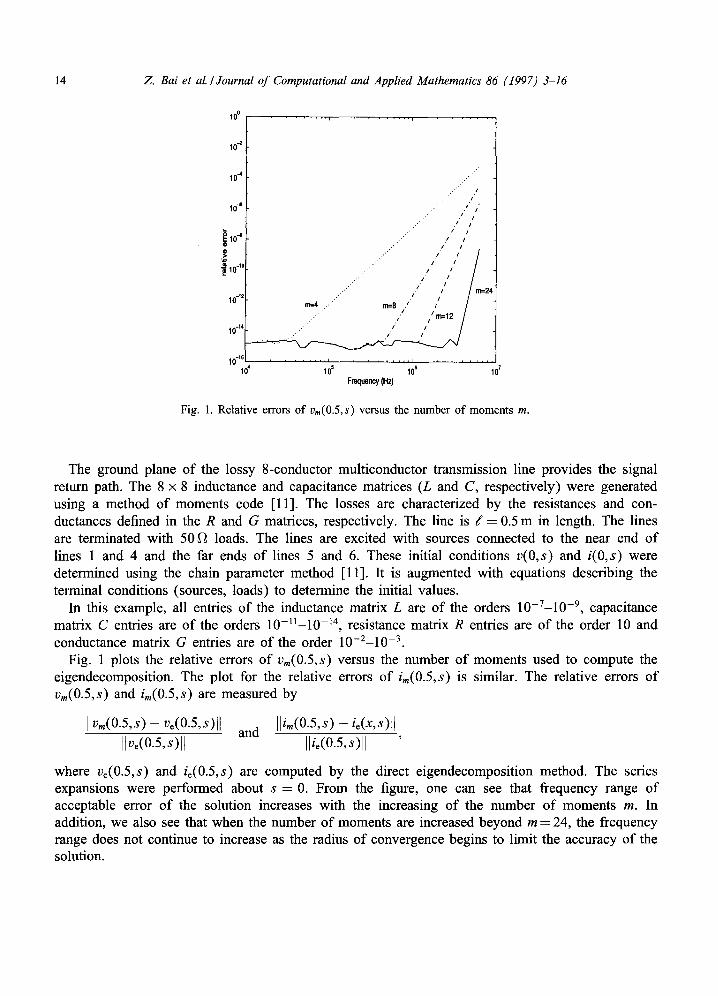
Fig. 2. Relatives errors of v,,(0.5,s) (top curve with "o") and the backward errors of the eigendecomposition of M(s), m= 12.
0.11
0.105
~ 0.1 ® ~0.095
0.0~
0.085
V_l(0.5,s}
i i i i i i i i
2 3 4 5 6 7 8 9 10
x 10 ~
| J:: o.
> -4 i i L i i i i i
2 3 4 5 6 7 8 9 10 Frequency (Hz) x 10 9
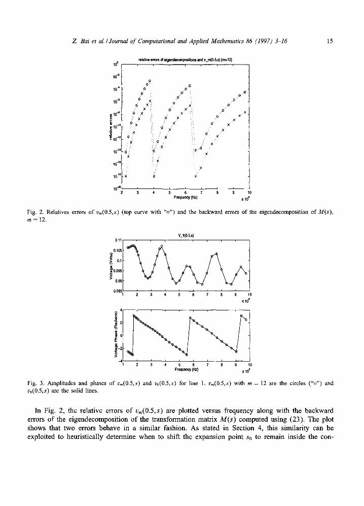
Fig. 3. Amplitudes and phases of /)m(0.5,S) and ve(O.5,s) for line 1. v,,(0.5,s) with m = 12 are the circles ("o") and ve(0.5,s) are the solid lines.
In Fig. 2, the relative errors o f vm(O.5,s) are plotted versus frequency along with the backward errors o f the eigendecomposit ion o f the transformation matrix M(s) computed using (23) . The plot shows that two errors behave in a similar fashion. As stated in Section 4, this similarity can be exploited to heuristically determine when to shift the expansion point So to remain inside the con-
16 z. Bai et al./ Journal of Computational and Applied Mathematics 86 (1997) 3-16
vergence radius when calculating the moments. This ensures that the moment solution will remain accurate over a broad range of frequencies.
Fig. 3 shows the plots of the far-end voltage amplitudes and phases of line 1 (Vl(0.5,s)). The volt- ages are computed using both the direct method (eigendecomposition computed for each frequency) and the moment matching method as implemented using the recursion algorithm from Section 3 and the expansion point shifting described in Section 4. The moment matching method shows excellent agreement with the direct method over the extremely large range of frequencies evaluated for this example. Similarly, the results for the other voltages and the currents also exhibited excellent agree- ment between the two methods. The agreement provides validation that the approximate moment matching method is a competitive approach for efficiently solving the MTL equations in frequency domain.
6. Concluding remarks
By exploiting the structure of the eigendecomposition of the transformation matrix M(s) , an efficient algorithm is developed to solve the MTL equations over a wide range of frequencies. This algorithm could be an order of magnitude faster than the existing direct methods. The accuracy of numerical results of interconnect models is very encouraging over a wide range of frequencies up to 10 GHz. It remains an open problem to determine an a priori convergence radius and rate of the series expansions of eigenvectors and eigenvectors for the transformation matrix M(s) .
References
[1] E. Anderson, Z. Bai, C. Bischof, J. Demmel, J. Dongarra, J. Du Croz, A. Greenbaum, S. Hammarling, A. McKenney, S. Ostrouchov, D. Sorensen, LAPACK Users' Guide, 2nd ed., SIAM, Philadelphia, 1995.
[2] G.A. Baker Jr., Essentials of Pad6 Approximation, Academic Press, New York, 1975. [3] J.E. Bracken, V. Raghavan, R.A. Rohrer, Interconnect simulation with asymptotic waveform evaluation (awe), IEEE
Trans. Circuits Systems 39 (1992) 869-878. [4] F.Y. Chang, The generalized method of characteristics for waveform relaxation analysis of lossy coupled transmission
lines, IEEE Trans. Microwave Technol. MMT-37 (1989) 2028-2038. [5] E. Chiprout, M.S. Nakhla, Asymptotic Waveform Evaluation, Kluwer Academic Publishers, Dordrecht, MA, 1994. [6] E. Coddington, N. Levinson, Theory of Ordinary Differential Equations, McGraw-Hill, New York, 1955. [7] R. Courant, D. Hilbert, Methods of Mathematical Physics, vol. I, Interscience, New York, 1953. [8] G. Golub, C. Van Loan, Matrix Computations, 2nd ed., Johns Hopkins University Press, Baltimore, MD, 1989. [9] T. Kato, Perturbation Theory for Linear Operators, 2nd ed., Springer, Berlin, 1980.
[10] T.W. Krrner, Fourier Analysis, Cambridge University Press, Cambridge, 1988. [11] C.R. Paul, Analysis of Multiconductor Transmission Lines, Wiley-Interscience, Singapore, 1994. [12] L.T. Pillage, R.A. Rohrer, Asymptotic waveform evaluation for timing analysis, IEEE Trans. Computer-Aided Design
9 (1990) 353-366.