Molecular Sturmians. Part 1

Molecular Sturmians. Part 1∗

JOHN AVERY, RUNE SHIMH.C. Ørsted Institute, University of Copenhagen, Department of Chemistry, Universitetsparken 5,DK-2100 Copenhagen O, Denmark

Received 22 January 2001; accepted 23 January 2001

ABSTRACT: Sturmian methods for solving the Schrödinger equation for an electronmoving in the field of a number of nuclei are reviewed. The problem is approached indirect space, although momentum-space techniques, including the use of hypersphericalharmonics, are used to evaluate the necessary integrals. In Part 2, these many-centerone-electron solutions, with weighted potentials, will be used to build up correlatedsolutions to the many-electron Schrödinger equations of molecules. c© 2001 John Wiley &Sons, Inc. Int J Quantum Chem 83: 1–10, 2001

Key words: quantum theory; Sturmians; hyperspherical harmonics; molecular orbitals;momentum spack

Introduction

D uring the early years of quantum chemistry itwas thought that hydrogenlike orbitals might

be used as basis sets for building up the wave func-tions of more complicated systems. However, it wasquickly realized that unless the continuum is in-cluded, such basis sets are not complete. To achievecompleteness, Shull and Löwdin [1] proposed thata type of radial basis set should be used that wouldconsist of an exponential factor, e−kr, multiplied by apolynomial in kr, the constant k being the same forall members of the set. They were able to show thatthis type of radial basis set is complete without theinclusion of the continuum. Subsequently, Roten-berg [2, 3], wishing to emphasize the connection of

∗This study is dedicated to the memory of Professor Per-OlovLöwdin, a great pioneer of quantum chemistry.

Correspondence to: J. Avery; e-mail: [email protected].

this type of basis with Sturm–Liouville theory, gavethem the name “Sturmians.” Sets of radial functionsof this type are currently very widely used in atomicphysics.

In 1968, Goscinski [4] introduced a powerful gen-eralization of the Sturmian concept. He defined aSturmian basis set as a solution of the Schrödingerequation with a weighted potential, the weightingfactor being chosen for each basis function in sucha way that all the members of the set correspondto the same value of the energy. In his 1968 work,Goscinski explicitly considered many-electron Stur-mian basis sets. Later, two-electron Sturmians wereused by Gazau and Maquet [5], while Bang and Vaa-gen and their co-workers [6, 7] introduced many-particle Sturmians into nuclear physics.

Sturmian basis sets are closely connected withmomentum-space quantum theory [8 – 13] and withthe theory of hyperspherical harmonics [14 – 59].Among the pioneering studies in momentum-spacequantum theory are some early articles by Pauling

International Journal of Quantum Chemistry, Vol. 83, 1–10 (2001)c© 2001 John Wiley & Sons, Inc.

AVERY AND SHIM

and Padolski [8] and by Coulson, McWeeny, andDuncanson [9 – 13]. The connection of momentum-space quantum theory with hyperspherical har-monics was made by Fock [14 – 16]. He was able toshow that it is possible to map three-dimensionalmomentum space onto the surface of a four-dimensional hypersphere in such a way that theFourier transforms of hydrogenlike orbitals can beexpressed very simply in terms of hypersphericalharmonics. The potential-weighted orthonormalityrelation obeyed by a Sturmian basis set can then berelated, through Fock’s mapping, to the orthonor-mality of the hyperspherical harmonics [38, 39].

Fock’s hyperspherical methods were extended tothe many-center one-electron problem by Shibuyaand Wulfman [17 – 19]. The method was further de-veloped by Monkhorst and Jeziorski [20], and itwas carried very far by Koga and his co-workers inJapan [22 – 31]. Significant developments in the the-ory are also due to Aquilanti and his co-workers atthe University of Perugia [34 – 36].

In the present work we shall review the meth-ods of Fock, Shibuya, and Wulfman for solving themany-center one-electron Schrödinger equation. InPart 2, we will show how potential-weighted many-center one-electron solutions can be used for build-ing up many-electron Sturmian basis sets of theGoscinski type. Also, in Part 2, we shall discuss howsuch a many-electron Sturmian basis set can be usedfor solving the many-electron Schrödinger equa-tion for a molecule directly, without the use of theHartree–Fock approximation. The present study be-gins with the direct-space one-electron Schrödingerequation. Its momentum-space counterpart is men-tioned only briefly, although Fourier transforms andhyperspherical harmonics are freely used in theevaluation of the necessary integrals.

Sturmian Solutions to the Many-CenterOne-Electron Problem

In quantum chemistry we are interested in themany-electron many-center Schrödinger equation.However, as a first step in constructing many-electron wave functions for molecules, we shall be-gin by solving the Schrödinger equation for a singleelectron moving in the attractive Coulomb poten-tial of the bare nuclei. In Part 2, we will show howthese solutions (with weighted potentials) can beused as building blocks for constructing multicon-figurational many-electron wave functions.

If we neglect magnetic and relativistic effects, thepotential experienced by an electron moving in theattractive field of the bare nuclei of a molecule is

v(x) = −∑

a

Za

|x− Xa| . (1)

Here x denotes the position of the electron while Za

and Xa represent the charges and positions of thenuclei. In atomic units, the Schrödinger equation foran electron moving in this potential can be writtenin the form [− 1

2∇2 + v(x)− ε]ϕµ(x) = 0. (2)

Letting

ε ≡ − 12 k2µ, (3)

we can rewrite the one-electron many-centerSchrödinger equation as[− 1

2∇2 + 12 k2µ + v(x)

]ϕµ(x) = 0. (4)

We can construct solutions to (4) from a set of atomicCoulomb Sturmian basis functions centered on thevarious nuclei:

ϕµ(x) =∑τ

χτ (x)Cτ ,µ, (5)

χτ (x) ≡ χnlm(x− Xa), (6)

where τ stands for the set of indices {anlm} and

χnlm(x) = Rnl(r)Ylm(θ ,φ), (7)

Rnl(r)=Nnl(2kµr)le−kµrF(l+ 1− n|2l+ 2|2kµr

),

Nnl =2k3/2µ

(2l+ 1)!

√(l+ n)!

n(n− l− 1)!.

(8)

In Eq. (8), F(a|b|x) = 1 + ax/b + a(a + 1)x2/(b(b +1)2!) + · · · is a confluent hypergeometric function.Table I shows the first few atomic Sturmian radialfunctions. They are the same as the familiar hydro-genlike radial functions, except that the factor Z/n,which appears in the hydrogenlike radial functions,has been replaced by kµ.

The atomic Coulomb Sturmians defined byEqs. (7) and (8) have the following properties [39]:[

−12∇2 + 1

2k2µ −

nkµr

]χnlm(x) = 0, (9)

∫d3xχ∗n′l′m′ (x)χnlm(x)

1r= kµ

nδn′nδl′lδm′m, (10)

and ∫d3x

∣∣χnlm(x)∣∣2 = 1. (11)

2 VOL. 83, NO. 1

MOLECULAR STURMIANS

TABLE ISturmian radial functions.

R10(r) = 2k3/2µ e−kµr

R20(r) = 2k3/2µ (1− kµr)e−kµr

R21(r) = 2k5/2µ√3

re−kµr

R30(r) = 2k3/2µ (1− 2kµr + 2k2

µr2

3 )e−kµr

R31(r) = (2kµ)5/2

3 r (1− kµr2 )e−kµr

R32(r) = 23/2k7/2µ

3√

5r2e−kµr

Introducing the expansion (5) into the many-centerone-electron Schrödinger equation, we obtain∑

τ

[− 12∇2 + 1

2 k2µ + v(x)

]χτ (x)Cτ ,µ = 0. (12)

We next multiply (12) on the left by a conjugatefunction from the basis set and integrate over thecoordinates of the electron. This gives us the set ofsecular equations:∑τ

∫d3xχ∗τ ′(x)

[− 12∇2 + 1

2 k2µ + v(x)

]χτ (x)Cτ ,µ = 0.

(13)

Momentum-Space Representationsof the Basis Set

In evaluating the matrix elements that occur inthe set of secular equations (13), it is convenientto make use of the momentum-space properties ofatomic Coulomb Sturmians. We therefore introducethe Fourier transforms:

χnlm(x) = 1(2π)3/2

∫d3p eip·xχ t

nlm(p),(14)

χ tnlm(p) = 1

(2π)3/2

∫d3x e−ip·xχnlm(x),

and

χτ (x) = 1(2π)3/2

∫d3p eip·xχ t

τ (p),(15)

χ tτ (p) = 1

(2π)3/2

∫d3x e−ip·xχτ (x).

From (6), (14), and (15) it follows that

χ tτ (p) = e−ip·Xa χ t

nlm(p) (16)

and that[− 12∇2 + 1

2 k2µ

]χτ (x) = 1

(2π)3/2

∫d3p eip·x

×(k2

µ + p2

2

)χ tτ (p). (17)

If we multiply (17) from the left by a conjugatefunction from our basis set and integrate over theelectron’s coordinates, making use of (15), we obtainthe relationship:∫

d3xχ∗τ ′(x)[− 1

2∇2 + 12 k2µ

]χτ (x)

=∫

d3p(

k2µ + p2

2

)×(

1(2π)3/2

∫d3x e−ip·xχ t

τ ′ (x))∗χ tτ (p)

=∫

d3p(k2

µ + p2

2

)χ t*τ ′ (p)χ t

τ (p) ≡ k2µSτ ′,τ . (18)

The matrix Sτ ′,τ defined by Eq. (18) will play animportant role in the solution of the many-centerone-electron problem. As we shall see, it is easy toevaluate, using the methods based on the work ofFock, Shibuya, and Wulfman; and it is closely re-lated to the other matrix, which occurs in the set ofsecular equations—the matrix involving v(x).

Fock’s Projection andHyperspherical Harmonics

Fock [14, 15] introduced the following projection,which maps three-dimensional momentum spaceonto the surface of a four-dimensional unit hyper-sphere:

u1 = 2kµp1

k2µ + p2 = sinχ sin θp cos φp,

u2 = 2kµp2

k2µ + p2 = sinχ sin θp sin φp,

(19)u3 = 2kµp3

k2µ + p2 = sinχ cos θp,

u4 = cosχ .

It is easy to see from the set of equations (19)that u2

1 + u22 + u2

3 + u24 = 1; and thus the four

quantities can be thought of as components of afour-dimensional unit vector defining a point on aunit hypersphere embedded in a four-dimensionalspace. Each point in momentum space correspondsto a point on the hypersphere. Fock was able to

INTERNATIONAL JOURNAL OF QUANTUM CHEMISTRY 3

AVERY AND SHIM

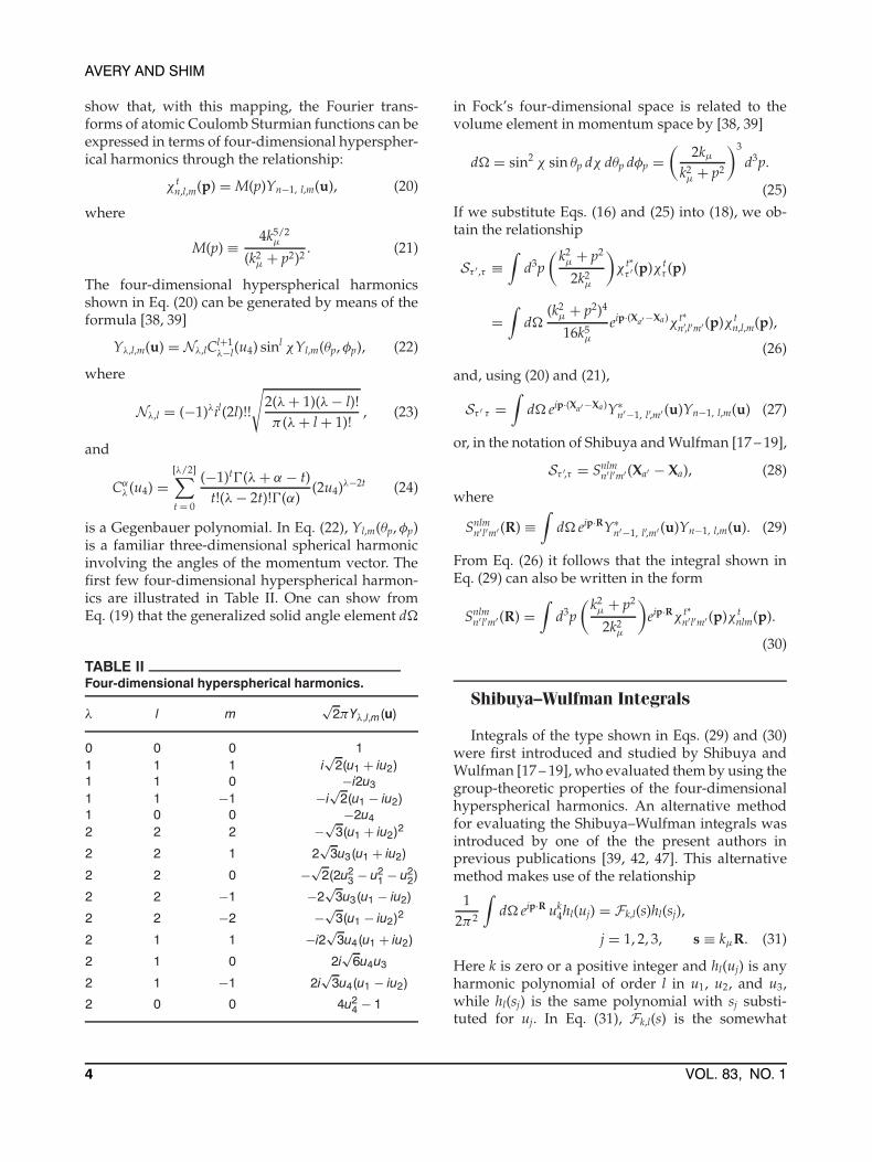
show that, with this mapping, the Fourier trans-forms of atomic Coulomb Sturmian functions can beexpressed in terms of four-dimensional hyperspher-ical harmonics through the relationship:

χ tn,l,m(p) =M(p)Yn−1, l,m(u), (20)

where

M(p) ≡ 4k5/2µ

(k2µ + p2)2 . (21)

The four-dimensional hyperspherical harmonicsshown in Eq. (20) can be generated by means of theformula [38, 39]

Yλ,l,m(u) = Nλ,lCl+1λ−l(u4) sinl χYl,m(θp,φp), (22)

where

Nλ,l = (−1)λil(2l)!!

√2(λ+ 1)(λ− l)!π(λ+ l+ 1)!

, (23)

and

Cαλ(u4) =[λ/2]∑t = 0

(−1)t0(λ+ α − t)t!(λ− 2t)!0(α)

(2u4)λ−2t (24)

is a Gegenbauer polynomial. In Eq. (22), Yl,m(θp,φp)is a familiar three-dimensional spherical harmonicinvolving the angles of the momentum vector. Thefirst few four-dimensional hyperspherical harmon-ics are illustrated in Table II. One can show fromEq. (19) that the generalized solid angle element d�

TABLE IIFour-dimensional hyperspherical harmonics.

λ l m√

2πYλ,l,m(u)

0 0 0 11 1 1 i

√2(u1 + iu2)

1 1 0 −i2u31 1 −1 −i

√2(u1 − iu2)

1 0 0 −2u42 2 2 −√3(u1 + iu2)2

2 2 1 2√

3u3(u1 + iu2)

2 2 0 −√2(2u23 − u2

1 − u22)

2 2 −1 −2√

3u3(u1 − iu2)

2 2 −2 −√3(u1 − iu2)2

2 1 1 −i2√

3u4(u1 + iu2)

2 1 0 2i√

6u4u3

2 1 −1 2i√

3u4(u1 − iu2)

2 0 0 4u24 − 1

in Fock’s four-dimensional space is related to thevolume element in momentum space by [38, 39]

d� = sin2 χ sin θp dχ dθp dφp =(

2kµk2µ + p2

)3

d3p.

(25)If we substitute Eqs. (16) and (25) into (18), we ob-tain the relationship

Sτ ′ ,τ ≡∫

d3p(k2

µ + p2

2k2µ

)χ t*τ ′ (p)χ t

τ (p)

=∫

d�(k2µ + p2)4

16k5µ

eip·(Xa′−Xa)χ t*n′,l′m′ (p)χ t

n,l,m(p),

(26)

and, using (20) and (21),

Sτ ′ τ =∫

d� eip·(Xa′−Xa)Y∗n′−1, l′,m′ (u)Yn−1, l,m(u) (27)

or, in the notation of Shibuya and Wulfman [17 – 19],

Sτ ′,τ = Snlmn′l′m′ (Xa′ − Xa), (28)

where

Snlmn′l′m′ (R) ≡

∫d� eip·RY∗n′−1, l′,m′ (u)Yn−1, l,m(u). (29)

From Eq. (26) it follows that the integral shown inEq. (29) can also be written in the form

Snlmn′l′m′ (R) =

∫d3p

(k2µ + p2

2k2µ

)eip·Rχ t*

n′l′m′ (p)χ tnlm(p).

(30)

Shibuya–Wulfman Integrals

Integrals of the type shown in Eqs. (29) and (30)were first introduced and studied by Shibuya andWulfman [17 – 19], who evaluated them by using thegroup-theoretic properties of the four-dimensionalhyperspherical harmonics. An alternative methodfor evaluating the Shibuya–Wulfman integrals wasintroduced by one of the the present authors inprevious publications [39, 42, 47]. This alternativemethod makes use of the relationship

12π2

∫d� eip·R uk

4hl(uj) = Fk,l(s)hl(sj),

j = 1, 2, 3, s ≡ kµR. (31)

Here k is zero or a positive integer and hl(uj) is anyharmonic polynomial of order l in u1, u2, and u3,while hl(sj) is the same polynomial with sj substi-tuted for uj. In Eq. (31), Fk,l(s) is the somewhat

4 VOL. 83, NO. 1

MOLECULAR STURMIANS

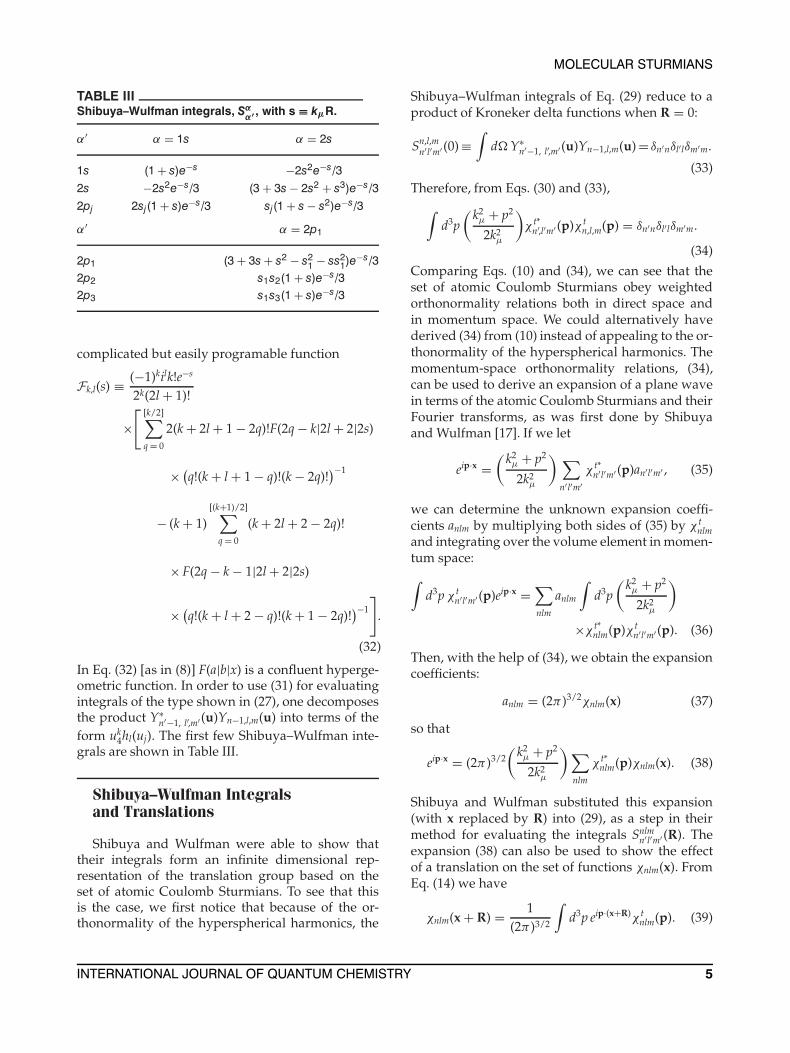
TABLE IIIShibuya–Wulfman integrals, Sα

α′ , with s ≡ kµR.

α′ α = 1s α = 2s

1s (1+ s)e−s −2s2e−s/32s −2s2e−s/3 (3+ 3s− 2s2 + s3)e−s/32pj 2sj(1+ s)e−s/3 sj(1+ s− s2)e−s/3

α′ α = 2p1

2p1 (3+ 3s+ s2 − s21 − ss2

1)e−s/32p2 s1s2(1+ s)e−s/32p3 s1s3(1+ s)e−s/3

complicated but easily programable function

Fk,l(s) ≡ (−1)kilk!e−s

2k(2l+ 1)!

×[ [k/2]∑

q= 0

2(k+ 2l+ 1− 2q)!F(2q− k|2l+ 2|2s)

× (q!(k+ l+ 1− q)!(k− 2q)!)−1

− (k+ 1)[(k+1)/2]∑

q= 0

(k+ 2l+ 2− 2q)!

× F(2q− k− 1|2l+ 2|2s)

× (q!(k+ l+ 2− q)!(k+ 1− 2q)!)−1

].

(32)

In Eq. (32) [as in (8)] F(a|b|x) is a confluent hyperge-ometric function. In order to use (31) for evaluatingintegrals of the type shown in (27), one decomposesthe product Y∗n′−1, l′,m′(u)Yn−1,l,m(u) into terms of theform uk

4hl(uj). The first few Shibuya–Wulfman inte-grals are shown in Table III.

Shibuya–Wulfman Integralsand Translations

Shibuya and Wulfman were able to show thattheir integrals form an infinite dimensional rep-resentation of the translation group based on theset of atomic Coulomb Sturmians. To see that thisis the case, we first notice that because of the or-thonormality of the hyperspherical harmonics, the

Shibuya–Wulfman integrals of Eq. (29) reduce to aproduct of Kroneker delta functions when R = 0:

Sn,l,mn′l′m′ (0)≡

∫d�Y∗n′−1, l′,m′(u)Yn−1,l,m(u)= δn′nδl′lδm′m.

(33)

Therefore, from Eqs. (30) and (33),∫d3p

(k2µ + p2

2k2µ

)χ t*

n′,l′m′ (p)χ tn,l,m(p) = δn′nδl′lδm′m.

(34)

Comparing Eqs. (10) and (34), we can see that theset of atomic Coulomb Sturmians obey weightedorthonormality relations both in direct space andin momentum space. We could alternatively havederived (34) from (10) instead of appealing to the or-thonormality of the hyperspherical harmonics. Themomentum-space orthonormality relations, (34),can be used to derive an expansion of a plane wavein terms of the atomic Coulomb Sturmians and theirFourier transforms, as was first done by Shibuyaand Wulfman [17]. If we let

eip·x =(k2

µ + p2

2k2µ

) ∑n′l′m′

χ t*n′l′m′ (p)an′l′m′ , (35)

we can determine the unknown expansion coeffi-cients anlm by multiplying both sides of (35) by χ t

nlmand integrating over the volume element in momen-tum space:∫

d3pχ tn′l′m′ (p)eip·x =

∑nlm

anlm

∫d3p

(k2µ + p2

2k2µ

)×χ t*

nlm(p)χ tn′l′m′(p). (36)

Then, with the help of (34), we obtain the expansioncoefficients:

anlm = (2π)3/2χnlm(x) (37)

so that

eip·x = (2π)3/2(k2

µ + p2

2k2µ

)∑nlm

χ t*nlm(p)χnlm(x). (38)

Shibuya and Wulfman substituted this expansion(with x replaced by R) into (29), as a step in theirmethod for evaluating the integrals Snlm

n′l′m′ (R). Theexpansion (38) can also be used to show the effectof a translation on the set of functions χnlm(x). FromEq. (14) we have

χnlm(x+ R) = 1(2π)3/2

∫d3p eip·(x+R)χ t

nlm(p). (39)


AVERY AND SHIM

Substituting (38) into (39), we obtain

χn,l,m(x+ R) =∑n′l′m′

χn′l′m′ (x)∫

d3p(k2

µ + p2

2k2µ

)× eip·Rχ t*

n′l′m′ (p)χ tnlm(p). (40)

The integral on the right-hand side of (40) can berecognized as a Shibuya–Wulfman integral (30), andthus we can write

χnlm(x+ R) =∑

n′l′m′χn′l′m′ (x)Snlm

n′l′m′ (R). (41)

Equation (41) implies the group property:

Snlmn′l′m′ (R+ R′) =

∑n′′l′′m′′

Sn′′l′′m′′n′l′m′ (R)Snlm

n′′l′′m′′ (R′). (42)

Multiplying Eq. (40) by χ∗n′′ ,l′′,m′′ (x), and integratingover the electron’s coordinates, making use of theorthonormality relation (10), we obtain:

Snlmn′′ l′′m′′ (R) = n′′

kµ

∫d3xχ∗n′′ ,l′′,m′′ (x)

1rχn,l,m(x+R). (43)

Thus the Shibuya–Wulfman integrals can also be in-terpreted as a type of nuclear attraction integral.

Sturmian Secular Equations

If we let

Vτ ′ ,τ ≡ − 1kµ

∫d3xχ∗τ ′(x)v(x)χτ(x), (44)

where v(x) is the many-center Coulomb attractionpotential defined by Eq. (1), then, making use ofEq. (18) and dividing by kµ, we can rewite the Stur-mian secular equations (13) in the form∑

τ

[Vτ ′,τ − kµSτ ′ ,τ ]Cτ ,µ = 0. (45)

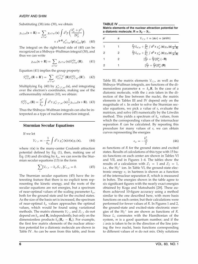
The Sturmian secular equations (45) have the in-teresting feature that there is no explicit term rep-resenting the kinetic energy, and the roots of thesecular equations are not energies, but a spectrumof near-optimal values of the scaling parameter kµ,both for the ground state and for the excited states.As the size of the basis set is increased, the spectrumof near-optimal kµ values approaches the optimalvalues, which would be found using variationalmethods. The matrix elements Vτ ′ ,τ and Sτ ′ ,τ do notdepend on kµ and Ra independently, but only on thedimensionless products kµ(Ra′ − Ra). For example,the first few matrix elements of the nuclear attrac-tion potential for a diatomic molecule are shown inTable IV. As can be seen from this table, and from

TABLE IVMatrix elements of the nuclear attraction potential fora diatomic molecule; R ≡ X2 − X1.

a′ a Vτ ′,τ τ ≡ {aα} ≡ {anlm}

1 1 Z1n δα′,α + Z2

kµ

∫d3 xχ∗

α′ (x)χα(x) 1|x−R|

2 2 Z2n δα′,α + Z1

kµ

∫d3 xχ∗

α′ (x)χα(x) 1|x+R|

1 2 [ Z1n′ + Z2

n ]Sαα′ (−R)

2 1 [ Z1n + Z2

n′ ]Sαα′ (R)

Table III, the matrix elements Vτ ′,τ , as well as theShibuya–Wulfman integrals, are functions of the di-mensionless parameter s = kµR. In the case of adiatomic molecule, with the z axis taken in the di-rection of the line between the nuclei, the matrixelements in Tables III and IV depend only on themagnitude of s. In order to solve the Sturmian sec-ular equations, we pick a value of s, evaluate thematrices, and solve (45) numerically by the Löwdinmethod. This yields a spectrum of kµ values, fromwhich the corresponding values of the internuclearseparation R can be calculated. By repeating thisprocedure for many values of s, we can obtaincurves representing the energies

εµ = −k2µ

2(46)

as functions of R for the ground states and excitedstates. Results of calculations of this type with 15 ba-sis functions on each center are shown in Tables VIand VII, and in Figures 1–4. The tables show theresults of a calculation with Z1 = 1 and Z2 = 1,i.e., the H2

+ ion. In Table VI, the ground-state elec-tronic energy ε1 in hartrees is shown as a functionof the internuclear separation R, which is measuredin bohrs. The energies shown in the table agree tosix significant figures with the nearly exact energiesobtained by Koga and Matsuhashi [28]. These au-thors achieved 10-figure accuracy using a methodsimilar to the one described here, with more basisfunctions on each center, but their calculations wereperformed for fewer values of R. In Figures 1 and 2,the ground-state and excited-state electronic ener-gies of the H2

+ ion are shown as functions of R.Since Lz commutes with the Hamiltonian of thesystem, m is a good quantum number; and if thez axis is taken to be in the direction of the line join-ing the two nuclei, basis functions correspondingto different values of m do not mix. Only solutions

6 VOL. 83, NO. 1

MOLECULAR STURMIANS

TABLE VNuclear attraction integrals (calculated by expanding 1/|x− R| in terms of Legendre polynomials); s ≡ kµR.

α′ α Wαα′ (R) ≡ 1

kµ

∫d3 xχ∗

α′ (x)χα(x) 1|x−R|

1s 1s 1s − e−2s

s (1+ s)

1s 2s − 12s + e−2s

2s (1+ 2s+ 2s2)

1s 2pz1s2 − e−2s

s2 (1+ 2s+ 2s2 + s3)

2s 2s 1s − e−2s

2s (2+ 3s+ 2s2 + 2s3)

2s 2pz − 32s2 + e−2s

2s2 (3+ 6s+ 6s2 + 4s3 + 2s4)

2pz 2pz1s + 3

s3 − e−2s

2s3 (6+ 12s+ 14s2 + 11s3 + 6s4 + 2s5)

corresponding to m = 0 (i.e., σ orbitals) are shownin Figures 1–4. Figure 3 shows some of the higherexcited-state energies of the system with Z1 = 1and Z2 = 3, while Figure 4 shows these energies

TABLE VIGround-state electronic energy ε1 in hartrees as afunction of the internuclear separation R, measuredin bohrs, for the H2

+ ion.a

R ε1 R ε1 R ε1

0.1 −1.97824 2.1 −1.07832 4.2 −0.7789950.2 −1.92860 2.2 −1.05538 4.4 −0.7634230.3 −1.86668 2.3 −1.03371 4.6 −0.7492210.4 −1.80073 2.4 −1.01321 4.8 −0.7362590.5 −1.73496 2.5 −0.993817 5.0 −0.7244180.6 −1.67147 2.6 −0.975442 5.2 −0.7135920.7 −1.61118 2.7 −0.958022 5.4 −0.7036840.8 −1.55447 2.8 −0.941493 5.6 −0.6946080.9 −1.50137 2.9 −0.925800 5.8 −0.6862821.0 −1.45178 3.0 −0.910891 6.0 −0.6786341.1 −1.40550 3.1 −0.896718 6.2 −0.6715981.2 −1.36230 3.2 −0.883238 6.4 −0.6651131.3 −1.32197 3.3 −0.870410 6.6 −0.6591261.4 −1.28424 3.4 −0.858198 6.8 −0.6535861.5 −1.24898 3.5 −0.846566 7.0 −0.6484501.6 −1.21593 3.6 −0.835484 7.2 −0.6436781.7 −1.18492 3.7 −0.824921 7.4 −0.6392351.8 −1.15580 3.8 −0.814849 7.6 −0.6350871.9 −1.12841 3.9 −0.805245 7.8 −0.6312072.0 −1.10263 4.0 −0.796082 8.0 −0.627570

a The energies agree to six significant figures with the almostexact values that Koga and Matsuhashi [28] calculated at asmaller number of points, using a similar method with a largerbasis set. Koga and Matsuhashi’s values agree to 10 signifi-cant figures with the best values calculated using spheroidalcoordinates.

(as functions of R) for the system with Z1 = 1and Z2 = 10. As mentioned above, the extra workneeded to make these calculations is very slight,once the V and S matrices have been calculated andstored as functions of Z1, Z2, and s. Some difficultywith overcompleteness was encountered when us-ing so many basis functions, and for certain valuesof s we found it necessary to reduce the size of thefunction space.

TABLE VIISimilar to Table VI, except that it shows the energy asa function of the internuclear distance R for the firstexcited state of the H2

+ ion.

R ε2 R ε2 R ε2

0.1 −0.500667 2.1 −0.673886 4.2 −0.6923840.2 −0.502677 2.2 −0.679567 4.4 −0.6888890.3 −0.506046 2.3 −0.684425 4.6 −0.6851600.4 −0.510784 2.4 −0.688579 4.8 −0.6812720.5 −0.516884 2.5 −0.692075 5.0 −0.6772870.6 −0.524308 2.6 −0.694963 5.2 −0.6732530.7 −0.532975 2.7 −0.697292 5.4 −0.6692100.8 −0.542745 2.8 −0.699113 5.6 −0.6651880.9 −0.553435 2.9 −0.700470 5.8 −0.6612131.0 −0.564813 3.0 −0.701409 6.0 −0.6573031.1 −0.576622 3.1 −0.701988 6.2 −0.6534801.2 −0.588595 3.2 −0.702215 6.4 −0.6497401.3 −0.600494 3.3 −0.702141 6.6 −0.6460981.4 −0.612075 3.4 −0.701797 6.8 −0.6425601.5 −0.623161 3.5 −0.701212 7.0 −0.6391291.6 −0.633605 3.6 −0.700414 7.2 −0.6358071.7 −0.643308 3.7 −0.699427 7.4 −0.6325941.8 −0.652205 3.8 −0.698274 7.6 −0.6294911.9 −0.660267 3.9 −0.696976 7.8 −0.6264952.0 −0.667488 4.0 −0.695551 8.0 −0.623606


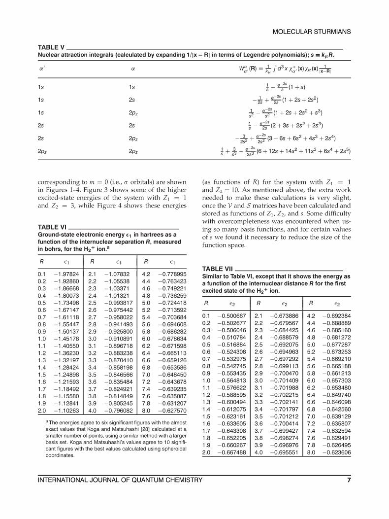
AVERY AND SHIM

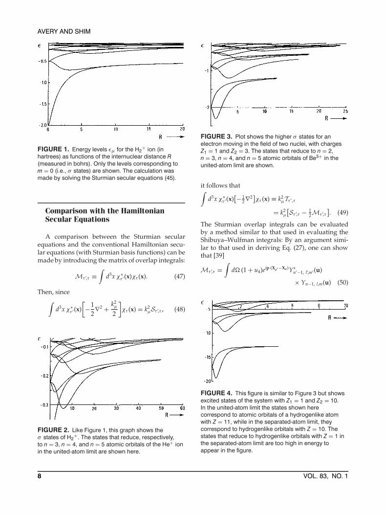
FIGURE 1. Energy levels εµ for the H2+ ion (in

hartrees) as functions of the internuclear distance R(measured in bohrs). Only the levels corresponding tom = 0 (i.e., σ states) are shown. The calculation wasmade by solving the Sturmian secular equations (45).

Comparison with the HamiltonianSecular Equations

A comparison between the Sturmian secularequations and the conventional Hamiltonian secu-lar equations (with Sturmian basis functions) can bemade by introducing the matrix of overlap integrals:

Mτ ′,τ ≡∫

d3xχ∗τ ′(x)χτ (x). (47)

Then, since∫d3xχ∗τ ′(x)

[−1

2∇2 + k2

µ

2

]χτ (x) = k2

µSτ ′,τ , (48)

FIGURE 2. Like Figure 1, this graph shows theσ states of H2

+. The states that reduce, respectively,to n = 3, n = 4, and n = 5 atomic orbitals of the He+ ionin the united-atom limit are shown here.

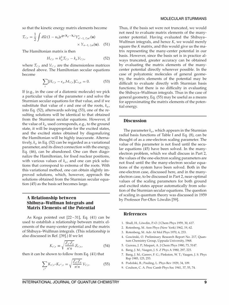
FIGURE 3. Plot shows the higher σ states for anelectron moving in the field of two nuclei, with chargesZ1 = 1 and Z2 = 3. The states that reduce to n = 2,n = 3, n = 4, and n = 5 atomic orbitals of Be3+ in theunited-atom limit are shown.

it follows that∫d3xχ∗τ ′(x)

[− 12∇2

]χτ (x) ≡ k2

µTτ ′ ,τ

= k2µ

[Sτ ′,τ − 1

2Mτ ′,τ]. (49)

The Sturmian overlap integrals can be evaluatedby a method similar to that used in evaluating theShibuya–Wulfman integrals: By an argument simi-lar to that used in deriving Eq. (27), one can showthat [39]

Mτ ′,τ =∫

d� (1+ u4)eip·(Xa′−Xa)Y∗n′−1, l′,m′(u)

× Yn−1, l,m(u) (50)

FIGURE 4. This figure is similar to Figure 3 but showsexcited states of the system with Z1 = 1 and Z2 = 10.In the united-atom limit the states shown herecorrespond to atomic orbitals of a hydrogenlike atomwith Z = 11, while in the separated-atom limit, theycorrespond to hydrogenlike orbitals with Z = 10. Thestates that reduce to hydrogenlike orbitals with Z = 1 inthe separated-atom limit are too high in energy toappear in the figure.

8 VOL. 83, NO. 1

MOLECULAR STURMIANS

so that the kinetic energy matrix elements become

Tτ ′,τ = 12

∫d� (1− u4)eip·(Xa′−Xa)Y∗n′−1, l′,m′ (u)

× Yn−1, l,m(u). (51)

The Hamiltonian matrix is then

Hτ ′,τ = k2µTτ ′,τ − kµVτ ′,τ , (52)

where Tτ ′,τ and Vτ ′ ,τ are the dimensionless matricesdefined above. The Hamiltonian secular equationsbecome ∑

τ

[Hτ ′,τ − εµMτ ′,τ ]Cτ ,µ = 0. (53)

If (e.g., in the case of a diatomic molecule) we picka particular value of the parameter s and solve theSturmian secular equations for that value, and if wesubstitute that value of s and one of the roots, kµ,into Eq. (52), afterwards solving (53), one of the re-sulting solutions will be identical to that obtainedfrom the Sturmian secular equations. However, ifthe value of kµ used corresponds, e.g., to the groundstate, it will be inappropriate for the excited states,and the excited states obtained by diagonalizingthe Hamiltonian will be highly inaccurate. Alterna-tively, kµ in Eq. (52) can be regarded as a variationalparameter, and its direct connection with the energy,Eq. (46), can be abandoned. One can then diago-nalize the Hamiltonian, for fixed nuclear positions,with various values of kµ, and one can pick solu-tions that correspond to extrema of the roots. Withthis variational method, one can obtain slightly im-proved solutions, which, however, approach thesolutions obtained from the Sturmian secular equa-tion (45) as the basis set becomes large.

A Relationship betweenShibuya–Wulfman Integrals andMatrix Elements of the Potential

As Koga pointed out [22 – 31], Eq. (41) can beused to establish a relationship between matrix el-ements of the many-center potential and the matrixof Shibuya–Wulfman integrals. (This relationship isalso discussed in Ref. [39].) If we let

Kτ ′,τ ≡√

Za′Za

n′nSτ ′,τ , (54)

then it can be shown to follow from Eq. (41) that∑τ ′′

Kτ ′,τ ′′Kτ ′′ ,τ =√

Za′Za

n′nVτ ′,τ . (55)

Thus, if the basis set were not truncated, we wouldnot need to evaluate matrix elements of the many-center potential. Having evaluated the Shibuya–Wulfman integrals, and hence K, we would merelysquare the K matrix, and this would give us the ma-trix representing the many-center potential in ourbasis. However, since the basis set is in practice al-ways truncated, greater accuracy can be obtainedby evaluating the matrix elements of the many-center potential directly wherever possible. In thecase of polyatomic molecules of general geome-try, the matrix elements of the potential may bedifficult to evaluate directly with Sturmian basisfunctions; but there is no difficulty in evaluatingthe Shibuya–Wulfman integrals. Thus in the case ofgeneral geometry, Eq. (55) may be useful as a meansfor approximating the matrix elements of the poten-tial energy.

Discussion

The parameter kµ, which appears in the Sturmianradial basis functions of Table I and Eq. (8), can bethought of as a one-electron scaling parameter. Thevalue of this parameter is not fixed until the secu-lar equations (45) have been solved. In the many-electron problem, which we shall discuss in Part 2,the values of the one-electron scaling parameters arenot fixed until the the many-electron secular equa-tions of the system have been solved. Both in theone-electron case, discussed here, and in the many-electron case, to be discussed in Part 2, near-optimalvalues of the scaling parameters for both groundand excited states appear automatically from solu-tion of the Sturmian secular equations. The questionof scaling in quantum theory was discussed in 1959by Professor Per-Olov Löwdin [59].

References

1. Shull, H.; Löwdin, P.-O. J Chem Phys 1959, 30, 617.2. Rotenberg, M. Ann Phys (New York) 1962, 19, 62.3. Rotenberg, M. Adv At Mol Phys 1970, 6, 233.4. Goscinski, O. Preliminary Research Report No. 217, Quan-

tum Chemistry Group, Uppsala University, 1968.5. Gazeau, J. P.; Maquet, A. J Chem Phys 1980, 73, 5147.6. Bang, J. M.; Vaagen, J. S. Z Phys A 1980, 297, 223.7. Bang, J. M.; Gareev, F. G.; Pinkston, W. T.; Vaagen, J. S. Phys

Rep 1985, 125, 253.8. Podolski, B.; Pauling, L. Phys Rev 1929, 34, 109.9. Coulson, C. A. Proc Camb Phys Soc 1941, 37, 55, 74.


AVERY AND SHIM

10. Coulson, C. A.; Duncanson, W. E. Proc Camb Phys Soc 1941,37, 67.

11. Duncanson, W. E. Proc Camb Phil Soc 1941, 37, 47.12. McWeeny, R.; Coulson, C. A. Proc Phys Soc (London) A

1949, 62, 509.13. McWeeny, R. Proc Phys Soc (London) A 1949, 62, 509.14. Fock, V. A. Z Phys 1935, 98, 145.15. Fock, V. A. Kgl Norske Videnskab Forh 1958, 31, 138.16. Bandar, M.; Itzyksen, C. Rev Mod Phys 1966, 38, 330, 346.17. Shibuya, T.; Wulfman, C. E. Proc Roy Soc A 1965, 286, 376.18. Wulfman, C. E. In Loebel, E. M., Ed. Group Theory and Its

Applications; Academic: New York, 1971.19. Judd, B. R. Angular Momentum Theory for Diatomic Mole-

cules; Academic: New York, 1975.20. Monkhorst, H. J.; Jeziorski, B. J Chem Phys 1979, 71, 5268.21. Navasa, J.; Tsoucaris, G. Phys Rev A 1981, 24, 683.22. Koga, T.; Murai, T. Theor Chim Acta 1984, 65, 311.23. Koga, T. J Chem Phys 1985, 82, 2022.24. Koga, T.; Matsumoto, S. J Chem Phys 1985, 82, 5127.25. Koga, T.; Kawaai, R. J Chem Phys 1986, 84, 5651.26. Koga, T.; Matsuhashi, T. J Chem Phys 1987, 87, 1677.27. Koga, T.; Matsuhashi, T. J Chem Phys 1987, 87, 4696.28. Koga, T.; Matsuhashi, T. J Chem Phys 1988, 89, 983.29. Koga, T.; Yamamoto, Y.; Matsuhashi, T. J Chem Phys 1988,

88, 6675.30. Koga, T.; Ougihara, T. J Chem Phys 1989, 91, 1092.31. Koga, T.; Horiguchi, T.; Ishikawa, Y. J Chem Phys 1991, 95,

1086.32. Duchon, C.; Dumont-Lepage, M. C.; Gazeau, J. P. J Chem

Phys 1982, 76, 445.33. Duchon, C.; Dumont-Lepage, M. C.; Gazeau, J. P. J Phys A:

Math Gen 1982, 15, 1227.34. Aquilanti, V.; Cavalli, S.; De Fazio, D.; Grossi, G. In Tsipis,

C. A.; Popov, V. S.; Herschbach, D. R.; Avery, J. S., Eds. NewMethods in Quantum Theory; Kluwer: Dordrecht, 1996.

35. Aquilanti, V.; Cavalli, S.; Coletti, C.; Grossi, G. Chem Phys1996, 209, 405.

36. Aquilanti, V.; Cavalli, S.; Coletti, C. Chem Phys 1997, 214, 1.

37. Wen, Z.-Y.; Avery, J. J Math Phys 1985, 26, 396.

38. Avery, J. Hyperspherical Harmonics; Applictions in Quan-tum Theory; Kluwer Academic: Dordrecht, 1989.

39. Avery, J. Hyperspherical Harmonics and Generalized Stur-mians; Kluwer Academic: Dordrecht, 2000.

40. Avery, J. In Problemes Non Lineaires Appliques, 1990-1991;Calcul Scientifique et Chimie Quantique; Écoles CEA-EDF-INRIA: Rocquencourt, France, 1991; pp. 1–28.

41. Avery, J. In Herschbach, D. R.; Avery, J.; Goscinski, O., Eds.Dimensional Scaling in Chemical Physics; Kluwer Acad-emic: Dordrecht, 1992; pp. 139–164.

42. Avery, J. In Kryachko, E. S.; Calais, J. L., Eds. ConceptualTrends in Quantum Chemistry, Vol. 1; Kluwer Academic:Dordrecht, 1994; pp. 135–169.

43. Avery, J. In Tsipis, C. A.; Popov, V.; Herschbach, D. R.; Avery,J., Eds. New Methods in Quantum Theory; Kluwer Acad-emic: Dordrecht, 1995.

44. Avery, J.; Herschbach, D. R. Int J Quantum Chem 1992, 41,673.

45. Avery, J. J Phys Chem 1993, 97, 2406.

46. Avery, J.; Antonsen, F. Theor Chim Acta 1993, 85, 33.

47. Avery, J. J Math Chem 1994, 15, 233.

48. Avery, J.; Børsen Hansen, T.; Wang, M.; Antonsen, F. Int JQuantum Chem 1996, 57, 401.

49. Avery, J.; Børsen Hansen, T. Int J Quantum Chem 1996, 60,201.

50. Aquilanti, V.; Avery, J. Chem Phys Lett 1997, 267, 1.


52. Avery, J.; Antonsen, F. J Math Chem 1998, 24, 175.

53. Avery, J. Adv Quantum Chem 1999, 31, 201.

54. Avery, J. J Mol Struct (Theochem) 1999, 458, 1.


56. Avery, J.; Sauer, S. In Hernández-Laguna, A.; Maruani, J.;McWeeney, R.; Wilson, S., Eds. Quantum Systems in Chem-istry and Physics, Vol. 1; Kluwer Academic: Dordrecht, 2000.

57. Avery, J.; Shim, R. Int J Quantum Chem 2000, 79, 1.

58. Weniger, E. J. J Math Phys 1985, 26, 276.

59. Löwdin, P. O. J Mol Spect 1959, 3, 46.

10 VOL. 83, NO. 1

Documents

Molecular Sturmians. Part 1