Embed Size (px)
Citation preview

Resource Use Efficiency as a Climate Smart Approach: Case of Smallholder Farmers in Nyando,
Kenya
by
Mohamud Suleiman Salat
A thesis submitted in partial fulfillment of the requirements for the degree of
Master of Science
In
Agricultural and Resource Economics
Department of Resource Economics and Environmental Sociology
University of Alberta
© Mohamud Suleiman Salat, 2017

ii
Abstract
To simultaneously enhance agricultural productivity and lower negative impacts on the
environment, food systems need to be transformed to become more efficient in using resources
such as land, water, and inputs. This study has examined the resource use efficiency of maize
production for smallholder farmers in Nyando, Kenya. The main objectives of this study were to
quantify the subplot level technical efficiency of the farmers while at the same time assessing the
impact of technologies, soil conservation practices and socio-economic characteristics on their
technical efficiency.
The study used Stochastic Frontier Analysis to simultaneously estimate a stochastic
production frontier and technical inefficiency effects models. The data used for this study were
mainly sourced from Climate Change Agriculture and Food Security (CCAFS) IMPACTlite data
collected in 2012. Data with panel structure on 324 subplots from 170 households were available
for this analysis.
The study revealed that maize production in Nyando is associated with mean technical
efficiency of 45% implying a scope of 55% for increasing production from the same areas of land.
Adoption of soil conservation practices such as residue management and legume intercropping
significantly increased technical efficiency. Use of plough and access to radio also significantly
increased technical efficiency.
In this area, agricultural policies aimed at tackling food security and climate change
challenges should focus on propagating the adoption of soil conservation practices such as residue
management and intercropping and productivity enhancing technologies such as improved seed
varieties.

iii
Preface
This thesis is an original work by Mohamud Salat. No part of this thesis has been previously
published.

iv
Dedication
This thesis book is dedicated to my wife Halima Abdille and my two sons Malik and Munir.

v
Acknowledgments
Firstly, I would like to thank the Almighty Allah for bestowing upon me a firm belief in His
oneness; giving me the opportunity to successfully complete my studies without major huddles,
for guiding and inspiring me throughout my thesis, for granting me physical and mental wellbeing,
patience and determination to face the challenges during my research. May He keep guiding me
throughout my entire life on this earth and make me one of the successful ones in the hereafter!
I would like to express my gratitude to my thesis supervisor, Professor Brent Swallow for
accepting to supervise my research, and providing continuous support and guidance from the
beginning to the end of this thesis work. His immense knowledge and expertise, suggestions and
contributions laid the foundations for me to develop and acquire critical and independent thinking
skills that will accompany me throughout my life. Thank you for playing such a big role in my
professional development!
I would like to extend my gratitude to my thesis committee member, Professor Scott Jeffrey
for being an integral part of this thesis and for initially guiding the scope of this research, for
patiently reviewing this thesis several times and providing very insightful comments and
suggestions. I would also like to thank my external examiner, Henry An for taking some time off
his busy schedule to examine and provide a critical review of this thesis.
My sincere appreciation goes to Climate Change Agriculture and Food Security (CCAFS)
program by Consultative Group on International Agricultural Research (CGIAR) for granting me
financial assistance and providing me with the data needed to carry out this research. I must also
thank David Pelster of International Livestock Research Institute (ILRI) who collaborated on this
research by providing extra data, advice, and helping with organizing a research trip to Kenya. My
appreciation goes to Joash Mango for his support during my field trip to Nyando, Kenya. I also
thank Joseph Sang of Jomo Kenyatta University of Agricultural technology (JKUAT) for
providing me with extra data.

vi
Finally, I extend my gratitude to all of my family members. I would like to thank my
mother, Abdiyo Shalle for being the most important person in my life, for being my source of
inspiration, guidance and advice throughout my entire life. To my brothers and sisters, thank you
for your support and prayers.
To my beautiful wife and best friend, the most amazing person in my life, Halima Abdille,
without whose encouragement and advice I would not have considered to pursue graduate studies.
Thank you for being a source of inspiration, a moral and spiritual support, and for your
resourcefulness and patience throughout my studies while taking care of our family. To my two
sons Malik and Munir, whose joy and smile provided me with energy and enlightenment after long
days of hard work and times of challenging experiences.

vii
Table of Contents
1 . Introduction ............................................................................................................................................. 1
1.1 Background ...................................................................................................................................... 1
1.2 Problem and Context........................................................................................................................ 3
1.3 Objectives ........................................................................................................................................ 5
1.4 Organization of Study ...................................................................................................................... 7
2 . Conceptual Framework and Previous Analytical Studies ................................................................... 8
2.1 The Concept of Efficiency in Economics ........................................................................................ 8
2.2 Approaches to Measuring Technical Efficiency ............................................................................ 12
2.3 Distributional Assumptions ........................................................................................................... 17
2.3.1 The Half-Normal Model ............................................................................................................ 17
2.3.2 The Exponential Model ............................................................................................................. 18
2.3.3 Truncated Normal Distribution Model ...................................................................................... 20
2.3.4 The Choice of Distribution ....................................................................................................... 22
2.4 Panel Data Models ......................................................................................................................... 23
2.5 Determinants of (In)efficiency ....................................................................................................... 26
2.6 Efficiency Studies in East Africa ................................................................................................... 27
2.7 Technology Adoption and Productivity ......................................................................................... 33
2.8 Soil Organic Carbon and Implications for Productivity ................................................................ 35
3 . Empirical Methods ................................................................................................................................ 39
3.1 Site Information ............................................................................................................................. 39
3.2 Data: Sources, Survey Design and Descriptive Statistics .............................................................. 42
3.3 Stochastic Frontier Analysis .......................................................................................................... 51
3.3.1 The Model and Assumptions ..................................................................................................... 51
3.3.2 Econometric Model ................................................................................................................... 53
3.4 Test for Skewness and Technique of Estimation ........................................................................... 59
3.5 Functional Forms ........................................................................................................................... 60
4 . Econometric Estimation and Results .................................................................................................. 62
4.1 Skewness of OLS residuals ............................................................................................................ 62
4.2 Choice of Functional Form and Discussion of Estimated Models ................................................. 65
4.3 Production Frontier Results and Discussion .................................................................................. 68
4.3.1 Coefficient Estimates of the Stochastic Production Frontier ..................................................... 68
4.3.2 Elasticities of Output and Returns to Scale ............................................................................... 69
4.4 Technical Efficiency and Determinants ......................................................................................... 71
4.4.1 Existence and Extent of Inefficiency ......................................................................................... 71
4.4.2 Equality of Means Test and Distribution of TE with Respect to Soil Conservation Practices .. 75
4.4.3 Determinants of Inefficiency ..................................................................................................... 78
4.5 Linking Soil Conservation Practices to Soil Capital ...................................................................... 82
5 . Summary and Conclusion .................................................................................................................... 84
5.1 Summary of Empirical Model ....................................................................................................... 84
5.2 Summary of Empirical Results ...................................................................................................... 84
5.3 Conclusion ..................................................................................................................................... 86
5.4 Limitations and Suggestions for Future Research ......................................................................... 88
References.................................................................................................................................................. 90
Appendices……………………………………………………………………………………………......97

viii
List of Tables
Table 2.1 Summary of Selected Efficiency Studies in East Africa ............................................................. 32
Table 3.1 Descriptive Statistics ................................................................................................................... 48
Table 3.2 Descriptive Statistics and Results of T-tests of Maize Yield by Management Practice ............. 49
Table 3.3 Correlation Matrix for the Variables Used in the Stochastic Production Function .................... 50
Table 3.4 Partial Correlations of the Variables Significantly Correlated with Maize Yield ....................... 50
Table 4.1 Results of OLS Regression ......................................................................................................... 64
Table 4.2 Likelihood Ratio Test Results* for Functional Forms................................................................. 66
Table 4.3 Coefficient Estimates for Parameters of the Cobb-Douglas Production Frontier ....................... 69
Table 4.4 Output Elasticities of Inputs ........................................................................................................ 71
Table 4.5 Likelihood Ratio Tests for the Hypotheses of Inefficiency Effects Model * .............................. 74
Table 4.6 Results of T-tests and Descriptive Statistics of TE by Soil Consertvation Practice ................... 77
Table 4.7 Partial Correlations of the Inefficiency Effects Variables with TE Estimates ............................ 79
Table 4.8 Results of the Determinants of TE for the Cobb-Douglas Formulation ..................................... 80
Table 4.9 Results of T-tests and Descriptive Statistics of Soil Carbon by Soil Conservation Practice ...... 83
Table A.1 Detailed Summary of OLS Residuals ........................................................................................ 97
Table A.2 Skewness/Kurtosis tests for Normality ...................................................................................... 98
Table B.1 Results of SPF Conventional and Simplified Translog Formulations…………………………99

ix
List of Figures
Figure 2.1 Illustration of Technical, Allocative and Economic Efficiency ................................................ 10
Figure 2.2 Stochastic Frontier Production Function. .................................................................................. 15
Figure 2.3 Half Normal Distribution........................................................................................................... 18
Figure 2.4 Exponential Distribution ............................................................................................................ 19
Figure 2.5 Truncated Normal Distribution ................................................................................................. 21
Figure 2.6 Technology Adoption and Productivity..................................................................................... 34
Figure 3.1 Location Map of Nyando ........................................................................................................... 41
Figure 3.2 Map of Nyando River Basin Showing the Three Blocks........................................................... 41
Figure 4.1 Frequency Density Plot of OLS Residuals ................................................................................ 63
Figure 4.2 Percentage Distribution of TE Scores. ..................................................................................... 75
Figure 4.3 Percentage Distribution of TE by soil Conservation Practice ................................................... 78
1
1 . Introduction
1.1 Background
Agriculture plays both victim and culprit roles in global climate change (FAO 2013). In its victim
roles, the sector is emerging to be the most vulnerable to the effects of climate change. The
characteristics of climate change include an increase in mean temperatures, changes in rainfall
patterns, increased variability in both the onset and amount of rainfall, and frequent occurrence of
extreme weather-related events such as droughts and floods. These changes are affecting
agricultural yields, making it more difficult for smallholder farmers in the tropics to grow certain
food crops such as maize, a staple food for most countries in Sub-Saharan African (SSA) (Agra.org
2014).
Small-scale farmers and pastoral communities in SSA, who are already resource scarce,
are facing localized climate change impacts that could push them to new poverty and hunger levels
(FAO 2013; Thornton and Lipper 2014). Empirical studies show that farmers in arid and semi-arid
areas of the region are already experiencing decreased growing seasons, lower yields and reduced
lands suitable for agriculture, mainly due to the warming climate (Collier et al. 2008). Moreover,
the human population of SSA is projected to grow to 1.5 billion by 2050 from its current 800
million, and this will mean a greater need for food production (Agra.org 2014).
Nonetheless, smallholder farmers are the backbone of the region's agricultural production,
comprising 80 percent of all farmers, and employing about 64 percent of the population (World
Bank 2007; Agra.org 2014). Under this reality, the stakes of climate change are higher for these
countries due to their high dependence on agriculture for food and cash income; and a lower
capacity to adapt to the changing climates (Collier et al. 2008; Bryan et al. 2011).
In its culprit roles, agriculture contributes to Green House Gas (GHG) emissions. IPCC
(2014) estimates that 24% of global anthropogenic GHG emissions are generated by agriculture,

2
forestry, and other land uses. Crop and animal farming contribute to emissions in a variety of
ways. For instance, various farm management practices such as fertilizer application, crop residue
management (crop residue burning), and land preparation lead to GHG emissions in the form of
carbon dioxide (CO2) and nitrous oxide (NO2) gases. In addition, emissions of carbon dioxide from
the soil mainly caused by agricultural practices such as soil cultivation, tillage, manure storage,
crop residue burning lead to the degradation of soil carbon stocks. Enteric fermentation by
ruminant animals releases a significant amount of methane gases into the atmosphere accounting
for about 40 percent of the total GHG emissions by the sector (FAO 2010b). As more lands are
cleared for agricultural production due to population pressures, these emissions are projected to
grow significantly. For instance, methane emissions from cattle and livestock manure are projected
to jump by 60 percent while nitrous oxide emissions will increase by 35-60 percent by 2030 (FAO
2013).
Policy makers and researchers are faced with three intertwined challenges with respect to
agriculture and climate change. These are climate change adaptation, mitigation of GHG
emissions, and food security. How can agriculture meet those challenges? There is need to
transform the sector to be able to address the intertwined challenges simultaneously. It is necessary
to study synergies and tradeoffs between the three challenges and build location specific evidence
through research. Perhaps most importantly, food systems need to be transformed to become more
efficient in using resources such as land, water, and inputs for sustainable production and at the
same time more resilient to climatic shocks (FAO 2013).
One of the most promising concepts so far is Climate Smart Agriculture (CSA). CSA was
first coined in the 2010 Hague conference on “Agriculture, Food Security, and Climate Change.”
The concept is defined as agriculture that simultaneously enhances productivity, enhances
resilience, and mitigates GHG emissions (FAO 2010). Examples of CSA practices are integrated
crop-livestock farming, use of improved crop varieties and animal breeds, meteorological weather
advisories, index-based insurance, soil conservation practices such as residue management, and
intercropping (FAO 2010).

3
Productivity can be defined as the ratio of output(s) produced to the input(s) used (Coelli et
al. 2005). Economic theory postulates changes in productivity arise from a combination of three
sources: technical change, technical efficiency change, and a change in scale of operations (Coelli
et al. 2005). An improvement in technical efficiency involves a movement towards the “best
practice” production. Technical change is realized when a firm produces more output(s) with the
same level of input(s) through a shift in the production frontier because of technological
improvement. A change in scale comes from an increase in firm’s scale of operations; and involves
a movement along the production function. While also capturing technical change, this study
mainly focusses on technical efficiency. More formal definitions and illustrations of these concepts
are provided in the next chapter.
1.2 Problem and Context
Most studies applying the concept of CSA have so far focused on specific practices such as those
mentioned above and their impact on farmer yield (Branca et al. 2011; Arslan et al. 2015).
Recently, we see mention of resource use efficiency as a climate smart approach (FAO 2013;
Thornton and Lipper 2014). According to FAO (2013), an increase in resource use efficiency is a
major key to reducing the intensity of GHG emissions per kilogram of output while also improving
food security, particularly in resource-limited areas such as SSA. However, little research exists
to link the efficiency literature with this new concept of farming. Most previous efficiency studies
in the region focussed on quantifying efficiency and examining the effects of socio-economic
factors such as income, age, and land size (Abate et al. 2014; Mburu et al. 2014). Little attention
has been paid to how best management agricultural practices affect efficiency. Using the case of
predominately maize-growing smallholder farmers in Kenya, this study measures farmers’
technical efficiency and examines how their efficiency is affected by the adoption soil conservation
practices such as residue management and intercropping. The study also examines the technical
impact of adopting improved seed varieties on productivity.
A key question then is: does a focus on technology and technical efficiency lead to different
intervention points than a focus on adoption of soil conservation practices and technologies
generally associated with Climate Smart Agriculture? Two specific questions stand out. First, are

4
there differences in technical efficiency that are related to the use of particular innovations or
access to information services? Second, are there agronomic technologies that achieve the goals
of climate smart agriculture through a shift in farmers’ production frontier (e.g. high-yielding
varieties)? For a particular area, the best approach to Climate Smart agricultural development will
depend on the answers to these questions as well as the local institutional and economic context.
The resource use efficiency approach is both a means to an end and an end in itself. While
it is a tool to measure farmers’ efficiency, the approach can also be used to study the effectiveness
of proposed soil conservation practices considered “climate smart”. According to FAO (2010),
some key climate smart practices with potential to increasing crop yields while also tackling
climate change challenges include soil nutrient management practices and use of seeds that are
better adapted to local agro-ecological conditions. Soils in most developing countries are depleted,
and the lost nutrients can be replaced through organic sources such as composting manure, crop
residues, and legume intercropping. These measures can increase soil organic matter while also
acting as an alternative to inorganic fertilizers whose transportation and storage contributes to
GHG emissions and farmer production costs (FAO 2010). Also, smallholder farmers should have
access to seed varieties that are better suited for local agro-ecological conditions (FAO 2010).
Many smallholder farmers are using crop varieties which are not adapted to erratic rainfall and
severe drought conditions. High yielding and early maturing crop varieties can address the
challenges of food security and climate change adaptations. As an end in itself, resource use
efficiency is a principal objective of CSA.

5
1.3 Objectives
The following are the main objectives of this study:
1. Estimate the production frontier of a sample of farmers in Nyando, Kenya and examine the
technological impact of adopting improved seed varieties on maize productivity.
2. Measure farmers’ subplot level technical efficiency.
3. Assess the impact of soil conservation practices namely residue management and
intercropping, and socio-demographic and -economic characteristics on subplot level
technical efficiency.
This study contributes to both efficiency and climate change literature, and the results are
significant in various ways. First, the technical efficiency measures can be used as a benchmark
for designing and implementing policies that enhance the agricultural productivity of farmers in
Western Kenya. An accurate assessment of efficiency and factors that affect it is necessary to
implement policies and institutional innovations that increase agricultural productivity (Sherlund
et al. 2002).
Second, the level of mean technical efficiency has implications for food security and
mitigation of GHG emissions. For instance, a low level of mean technical efficiency indicates that
farmers in Western Kenya are on average not utilizing farm inputs available to them in a way that
maximizes output and minimizes input waste. This means that productive inputs are not fully
exploited and that agricultural production is not in line with the principles of Climate Smart
agriculture. A low mean technical efficiency thus indicates a potential scope to improve farmers’
technical efficiency through policies such as an increase in use of conservation practices.
How can an improvement in technical efficiency lead to lower GHG emissions? As
mentioned earlier, agricultural production significantly contributes to GHG emissions that pose
global environmental consequences (McCarl and Schneider 2000). In economic terms, it means
that agricultural production is associated with negative externalities. A negative externality is

6
created when the action of one party (producers) imposes an external cost on another party (the
environment and society). The pressure on the environment caused by agricultural production such
as soil erosion, sedimentation and reduction of carbon sequestration1 due to the clearing of more
land for farming is in this case an external cost not accounted for in the production process. An
improvement in technical efficiency implies that more is produced with less of the resources and
activities responsible for emissions (e.g. less land is cultivated and less polluting inputs such as
fertilizer and pesticides are used), thus, internalizing this negative externality. The relationship
between efficiency improvement and GHG emissions is, however, ambiguous and depends on the
nature of other economic factors. The reduction in cultivated area due to improvements in
productive efficiency has been called the Borlaug hypothesis, after Norman Borlaug, who
postulated that an increase in per hectare agricultural yield will lead to a reduction in the demand
for more cropland, thus sparing forest lands (Rudel et al. 2009). According to Rudel et al. (2009),
this effect can only be true if the demand for farmers’ produce is inelastic and the price for the
product decreases (supply-side effect), thus reducing the incentive to clear more lands for
cultivation. However, if the farmers face an elastic demand, the increasing prices incentivise them
to increase the area under cultivation in order to get more profits. This phenomenon is called
Jevons Paradox, named after William Stanley Jevon, who saw that England’s growing efficiency
in coal usage in the 19th century increased rather than decreased its use (Rudel et al. 2009). Using
national level agricultural production and land use data from FAO for the periods 1970-2005 for
ten major crops. Rudel et al. (2009) found a pattern generally conforming to the Jevons Paradox:
a simultaneous rise in agricultural yields and area of land cultivated. Despite this general outcome,
their study reveals conformity to the Borlaug hypothesis for certain crops such as wheat and coffee;
and for particular regions of the world such as Anglo-America, Middle America and the Caribbean.
Third, the effectiveness of conservation practices under assessment can be used to build
location specific evidence of appropriate practices better positioned to meet the objectives of CSA.
Specifically, the indirect impact of these variables on productivity through their impact on TE can
be measured.
1 Carbon sequestration is defined as “transferring atmospheric CO2 into long lived pools and
storing securely so it is not immediately reemitted” (Lal. 2004 p.1623).

7
This study also contributes to an emerging body of efficiency literature that account for
inter-farm environmental and geographic heterogeneity. As will be discussed later, failing to
control for environmental factors in efficiency analysis can lead to omitted variable bias. For this
study, access to data on soil organic carbon, erosivity, precipitation and evapotranspiration will
enable me to capture more environmental heterogeneity than most previous efficiency studies have
been able to do.
The framework of Stochastic Frontier Analysis is used for this study. I have access to
Climate Change Agriculture and Food Security (CCAFS) IMPACTlite data collected in the year
2012 in 15 of CCAFS benchmark sites in 12 countries in Africa and South East Asia. CCAFS is a
research program by Consultative Group for International Agricultural Research (CGIAR) aimed
at addressing the challenges of food security and global warming through “agricultural practices,
policies, and measures” (CCAFS, https://ccafs.cgiar.org/). The IMPACTlite survey selected two
hundred households in each location through multi-stage random sampling. The survey collected
information on farmer’s agricultural practices and socio-demographic characteristics as well as
subplot-level information on farming activities taking place at different times of the year.
1.4 Organization of Study
The rest of the chapters are organized as follows. Chapter Two delves into the theoretical
frameworks and literature review. I define the concept of technical efficiency and discuss its
theoretical basis and existing frameworks for estimating TE. I then review some East African
studies (mainly focusing on Kenya) that examine efficiency of farmers. In addition, the technical
impact of new technology on productivity and the significance of soil organic carbon for
agronomic productivity are discussed in the last two sections of this chapter. Chapter three presents
the empirical methods. I start the chapter with a brief introduction to the study site followed by a
discussion of the data (sources, construction of variables, descriptive and exploratory statistics). I
then outline the econometric model used to fit the data, method of estimation, and functional forms.
Chapter Four presents and discusses the results of the estimated models. Chapter Five gives a
summary, conclusion and suggestions for further studies.

8
2 . Conceptual Framework and Previous Analytical Studies
This chapter discusses the theoretical and analytical frameworks in Stochastic Frontier Analysis
(SFA), discusses the measurement of technical efficiency (TE), reviews previous efficiency studies
in East Africa, and discusses the impacts of new technologies and soil organic carbon on
agronomic productivity. More specifically, Section 2.1 defines the concept of TE along with other
efficiency types and discusses the theoretical basis of TE; Section 2.2 discusses existing
frameworks for measuring TE, while Section 2.3 reviews distributional assumptions. Section 2.4
presents SFA and measurement of TE in a panel data context. Section 2.5 discusses the theory and
framework for studying determinants of TE. Section 2.6 provides a review of some of the existing
efficiency studies in East Africa. Section 2.7 discusses and illustrates how technology adoption
technically improves productivity through a shift in the production frontier. Section 2.8 discusses
the significance of soil carbon dynamics for agronomic productivity and the effect of soil
conservation practices on soil carbon dynamics.
2.1 The Concept of Efficiency in Economics
The concept of efficiency dates back to the early works of Koopmans (1951), Debreu (1951), and
Shephard (1953). Koopmans (1951) defined TE as the point at which it is impossible to produce
more of a given output without using more of some input or producing less of another output.
Debreu (1951), on the other hand, first provided a measure of efficiency through the “Coefficient
of Resource Utilization.” It was, however, Farrell (1957) who first empirically measured
productive efficiency. Following the works of Koopmans (1951) and Debreu (1951), Farrell
(1957) defined cost efficiency and showed how cost efficiency can be decomposed into its
components: TE and Allocative efficiency (AE). He then provided an empirical application to U.S
agriculture using linear programming techniques.
Efficiency concepts can be defined either using input-oriented (IO) or output-oriented (OO)
measurements. IO measures of efficiency focus on proportional reduction in inputs without

9
changing the output quantities, whereas OO measures focus on proportional expansion in outputs
without altering input quantities (Coelli et al. 2005). TE can be defined, using the IO measurement,
as the ability of a firm to use the minimum feasible quantities of inputs to produce a given level of
output2. Allocative efficiency can be defined as the ability of a firm to combine production inputs
in optimal proportions given their respective prices. A firm’s economic (cost) efficiency (EE) is a
combination of its technical and allocative efficiencies and can be measured by the product of TE
and AE.
Using Figure 2.1 and following Farrell (1957) and Coelli et al. (2005), I illustrate the
efficiency types defined above using an example of a farmer who uses only two inputs, X1 and X2,
to produce a single output, Y, under the assumption of constant returns to scale3. This illustration
is consistent with the IO definition of efficiency. I assume that this farmer has full knowledge of
the efficient production frontier4. HH’ is an isoquant representing the various combinations of the
two inputs that a 100% efficient farmer would use to produce a unit of output such that any point
on the isoquant is technically efficient. Point Q, for instance, is technically efficient. WW’ is an
isocost line representing the combination of the two inputs such that their individual costs add to
the same cost of production. Point Q’ represents the least cost combination of the two inputs, X1
and X2. Point Q’ is both technically and allocatively efficient since it is both on the isoquant and
is the least cost feasible point.
Suppose the farmer is producing at point P. At this point, the farmer is both technically
and allocatively inefficient. The distance QP measures the amounts by which inputs X1 and X2
could be reduced without reducing output to produce at the technically efficient point Q. The TE
of the farmer is measured by the ratio, OQ/OP, which is equal to one minus QP/OP. TE takes a
value between zero and one, where a value of one indicates full TE.
2 Alternatively, the concept can also be defined, using output-augmenting measurement, as the
ability to produce maximum output from a given input bundle. 3 The constant returns to scale condition enables us to represent the production technology in a
simple isoquant. 4 In practice, knowledge of the production frontier of full efficiency cannot be assumed, and,
hence should be estimated using sample data.

10
The distance RQ represents the amount by which the cost of production could be reduced
in order to produce at the allocatively efficient point Q’ instead of the technically efficient but
allocatively inefficient point Q. The ratio RQ/OQ represents the proportional reduction in the cost
of production required in reallocating inputs to move from Q to Q’. The allocative efficiency of
the farmer is thus the ratio OR/OQ.
The distance RP is the reduction in costs that would occur for the farmer to achieve both
technical and allocative efficiency (i.e. produce at point Q’) or become economically efficient in
other words. Thus, the economic efficiency of the farmer producing at P is given by the measure
OR/OP which is equally measured by the product of AE and TE. Thus, EE = AE x TE = (OR/OQ)
x (OQ/OP) = OR/OP
Figure 2.1 Illustration of Technical, Allocative and Economic Efficiency
IO and OO approaches give the same efficiency measurements only in the case of constant
returns to scale. In the literature, there is no correct choice of approach; however, parametric

11
stochastic frontier models (this will be discussed in the following sections) applying the standard
method of ML use the OO measure. The same models with IO measurement, on the other hand,
cannot be estimated using the standard ML method because the inefficiency error term in the
stochastic frontier model is heteroskedastic5 and the ML method needs to be extended to
accommodate this heteroscedasticity (Kumbhakar and Tsionas 2008). Kumbhakar and Tsionas
(2008) estimated non-homogeneous stochastic production frontier models using both OO and IO
approaches and found that the mean and spread of TE from the output-oriented model were higher
than those based on the input-oriented model. The study also reported differences in returns to
scale and output elasticities between the two models. According to Kumbhakar and Tsionas
(2008), the choice of either OO or IO is usually based on economic factors and the IO approach
might be preferred in the cases of regulated industries (e.g., output quota regulation). As the most
commonly used approach, the OO approach has been chosen for this study.
This study focusses only on TE and factors that affect it. While an examination of all
efficiency types would be even more useful, I am constrained by data limitations to focus only on
TE since the measurement of economic and allocative efficiency requires data on input and output
prices that were not available in this case.
The basis for TE lies in the theory of the production function. Consider a producer who
uses a vector of inputs X = (X1 … XN) to produce a single output Y. The producer transforms the
vector of inputs into an output according to a production function, f(X), a function that shows the
maximum feasible output that can be obtained from the set of inputs by an efficient producer. The
function, f(X), is referred to as a production frontier as it shows the maximum output attainable
from each input level. If the producer has a plan to produce Y* units of output using X* units of
inputs, the plan will be termed as technically efficient if f(X*) = Y*, and technically inefficient if
f(X*) < Y*.
5 Kumbhakar and Tsionas (2008) present and discuss stochastic frontier models with both IO and
OO measurements and show that the inefficiency error term in the IO stochastic frontier model is
a function of the input parameters.

12
Empirically, TE can be measured using sample data as the ratio of observed mean output to
the corresponding potential mean output that a fully efficient firm would obtain if it used all the
inputs efficiently.
2.2 Approaches to Measuring Technical Efficiency
Ever since Farrell (1957) attempted to measure efficiency, other researchers have been building
on his ideas about frontier modeling. Farrell used linear programming techniques to empirically
measure the concept. This technique influenced the development of Data Envelopment Analysis
(DEA), through the works of Charnes et al. (1978). DEA is now a well-established non-parametric
efficiency measurement technique, and although previously used in the management sciences, is
also widely applied in economics. DEA uses linear programming methods to construct a non-
parametric piecewise frontier that envelopes the data points such that for a production frontier, all
the observed points lie on or below the production frontier, whereas, for a cost frontier the observed
data points lie on or above the cost frontier (Coelli et al. 2005). Efficiency measures are then
calculated relative to the frontier.
Another competing approach to the non-parametric method is the use of parametric
methods where production or cost frontiers are estimated using econometric methods. This
method, unlike the non-parametric approach, imposes a functional form on the data. The
parametric methods have evolved into deterministic and stochastic methods. The deterministic
method attributes all deviations from the frontier as solely arising from the inefficiency of the
decision-making unit. The following general form defines the deterministic frontier model.
𝑌𝑖 = 𝑓(𝑋𝑖 ; 𝛽) 𝑒𝑥𝑝(−𝑢𝑖), 𝑢𝑖 ≥ 0 𝑖 = 1, 2, … , 𝑁 , (2. 1)
where Yi represents the output of the ith decision-maker; f(Xi ; β) is a suitable functional form to
represent a K x 1 vector, Xi , of inputs for the ith decision maker, and a 1 x K vector, 𝛽 , of unknown
parameters to be estimated; ui ≥ 0 is a non-negative random variable associated with the technical
inefficiency of the decision-making unit; and N is the number of decision making units.

13
Aigner and Chu (1968) first used this method by considering a Cobb-Douglas production
frontier and estimated the model using linear programming techniques. Their work involved
applying the technique to cross-sectional data by minimizing the sum of residuals. Winsten (1957)
proposed a Corrected Ordinary Least Squares (COLS) method to estimate the above model in two
steps. The first step involves estimating the model by Ordinary Least Squares (OLS) to obtain
consistent and unbiased slope parameter estimates, and a consistent but biased slope intercept
estimate (Kumbhakar and Lovell 2003). In the second step, the biased OLS intercept is corrected
by shifting it to have the estimated frontier bound the data points from above (Kumbhakar and
Lovell 2003). Afriat (1972) assumed that the uis had a gamma distribution and estimated the
above model by ML methods. Richmond (1974) assumed that the inefficiency error follows either
half-normal or exponential distribution and applied Modified Ordinary Least Squares (MOLS) to
estimate the above model. Like the COLS, this technique also follows a two-step procedure. The
model is estimated by OLS in the first step, and the resulting intercept is shifted up by the mean
of the previously assumed one-sided distribution.
The technical inefficiency of the ith decision maker is thus the amount by which its level of
output is less than its frontier output. Given the above model, let the frontier output be
Yi∗ = f( Xi ; β ). The TE of the ith decision maker is given by
𝑇𝐸 = 𝑌𝑖
𝑌𝑖∗ =
𝑓(𝑋𝑖 ; 𝛽) 𝑒𝑥𝑝(−𝑢𝑖)
𝑓(𝑋𝑖 ; 𝛽)= 𝑒𝑥𝑝(−𝑢𝑖). (2. 2)
A possible limitation of deterministic methods is that all deviations from the frontier are
attributed to technical inefficiency. A problem with this type of frontier model is that random
shocks outside of the control of the decision maker and measurement errors are not taken into
account (Coelli et al. 2005). The emergence of SFA addressed this drawback by introducing an
additional random variable to account for random shocks and measurement errors. Aigner et al.
(1977) and Meeusen and Van den Broeck (1977) independently proposed the stochastic production
frontier function model. The general form of the model is as follows
𝑌𝑖 = 𝑓(𝑋𝑖 ; 𝛽)𝑒𝑥 𝑝(𝑣𝑖 − 𝑢𝑖), 𝑢𝑖 ≥ 0 𝑖 = 1, 2, … , 𝑁. (2. 3)

14
The above model is similar to the deterministic model, except that a new symmetric random error
term, vi, has been added to account for random shocks and measurement errors. The model is such
that Yi is bounded from above by a stochastic quantity, f(Xi ; β)exp (vi); hence the name stochastic
frontier (Battese 1992). In addition, the first part of the model , f(Xi ; β) is called the deterministic
component. The second part, exp (vi − ui), consists of a noise component, 𝑣𝑖, assumed to be an
independently and identically distributed (iid) random variable, and inefficiency component, ui ≥
0 , assumed to be iid non-negative random variable that is independent of vi.
Using an example of two firms, C and D, that only use one type of input (Xi) each to
produce Yi units of output each ( i = C, D), I graphically illustrate in Figure 2.2, the general form
of the stochastic frontier model given above. The values of Xi are measured along the horizontal
axis, while the outputs are measured along the vertical axis. The deterministic part of the model is
drawn to reflect the existence of diminishing marginal returns.
The frontier output for firm C lies above the deterministic part of the production frontier
because the noise component is positive (vC > 0) and thus the productive activities of the firm is
associated with the occurrence of favourable conditions. The frontier output of firm D on the other
hand is below the deterministic part of the production frontier as its productive activities occur
under unfavourable conditions and thus the noise component is negative (vD < 0).
The observed output of each firm deviates from the frontier output by the size of the
technical inefficiency effect. For instance, firm C’s production is relatively inefficient as shown
by the distance between its actual observed output and its frontier output. Firm D’s production is
relatively less inefficient. Thus, the inefficiency effect of firm C is greater than the inefficiency
effect of firm D and therefore firm D is more technically efficient than firm C. The TE of each
firm is denoted by
TEi =Yi
Yi∗ =
f(Xi ; β) exp(vi − ui)
f(Xi ; β) exp(vi)= exp(−ui) (2. 4)

15
Figure 2.2 Stochastic Frontier Production Function.
Prediction of TE, denoted by TEi = exp(−ui) , i = 1, 2, . . . , N , involves decomposing
the combined random error, εi = vi − ui into its components, vi and ui to obtain firm specific
technical inefficiency effects which are then used to compute firm specific TE effects. The
decomposition process was impossible (due to the fact that the inefficiency error term is
unobservable) until the paper of Jondrow et al. (1982). The paper suggested a decomposition
procedure hereafter referred to as the JLMS technique, based on the conditional distribution of the
non-negative inefficiency error term, ui, given that the combined error term, εi = vi − ui , was
observable and could be estimated.
The procedure suggests that ui be predicted by the expectation of ui, conditional on εi.
Assuming half normal and exponential distributions for the uis, Jondrow et al. (1982) used the

16
formula 1 − E(ui|εi) to predict firm specific TE. However, Battese and Coelli (1988) suggested
that the TE of the ith decision maker is best predicted using the formula E(exp{−ui}|εi). This latter
formula has been evaluated for more general stochastic frontier models such as the truncated
normal and panel data models (Battese 1992).
Both DEA and SFA have widely been used in efficiency analysis and theory does not
favour one method over the other. Both have their strengths and weaknesses, and tradeoffs exist
in choosing, a priori, a particular approach (Hjalmarsson et al. 1996). Unlike DEA, SFA requires
the imposition of a functional form. This a priori imposition could be risky “given that most of the
distributional characteristics of the production technology are priori unknown” (Cullinane et al.
2006 p.356).
Also, SFA requires distributional assumptions on the error structure; an assumption that is
difficult to ascertain and could even introduce other sources of errors (Cullinane et al. 2006).
Compared to SFA, DEA does not impose a particular functional form nor does it require
assumptions on the error structure. In doing so, DEA lets the data “speak for themselves”
(Cullinane et al. 2006 p.356). Despite this, SFA is advantageous in that it accounts for the
influence of random factors that are outside of the decision maker’s control. Also, the use of SFA
enables one to perform formal statistical test of hypotheses and construct confidence intervals
(Hjalmarsson et al. 1996). While aware of the tradeoffs in choosing a particular approach, this
study uses the framework of SFA.
Estimation of stochastic production frontier models involves making distributional
assumptions on the error terms and applying the method of ML. A likelihood function is defined
and maximized with respect to the parameters of the stochastic frontier model. The ML estimators
have numerous desirable asymptotic properties (Coelli et al. 2005). The parameter estimates are
asymptotically consistent, meaning that their values approach their true population parameters and
variance gets smaller as the sample size approaches infinity. The estimates are also asymptotically
normally distributed meaning that the estimator converges to the true parameter fast enough (i.e.
asymptotic efficiency). For this reason, the ML estimator is preferred to other estimators used to
measure TE such as COLS.

17
Distributional assumptions lie at the heart of ML methods used to estimate stochastic
frontier models. It is an essential requirement to decompose the estimates of the composite error
term,εi, into its statistical components, ui and vi. In the following section, a brief discussion of the
most commonly used distributional assumptions is provided.
2.3 Distributional Assumptions
There are three distributional assumptions commonly used in the literature. These are the half-
normal, exponential, and truncated normal distributions. This section discusses stochastic frontier
models with these distributional assumptions. I briefly discuss these distributional assumptions.
The equations used here have been referenced from Kumbhakar and Lovell (2003) who provide a
detailed background of the three distributional assumptions.
2.3.1 The Half-Normal Model
Consider the stochastic frontier model specified in equation 2.2. The half-normal model assumes
that the uis are non-negative random variables distributed iid ~ 𝑁+(0, σu2), obtained by truncation
of the normal distribution 𝑁(0, 𝜎2) at zero. The model also assumes that the two error terms are
independently distributed of each other and of the explanatory variables. The half-normal
distribution of the inefficiency error term depends on its standard deviation parameter,σu. The
probability density function is given by
𝑓(𝑢) = 2
√2𝜋 𝜎𝑢
. 𝑒𝑥𝑝 ⌈−𝑢2
2𝜎𝑢2
⌉ , 𝑢 ≥ 0. (2. 5)
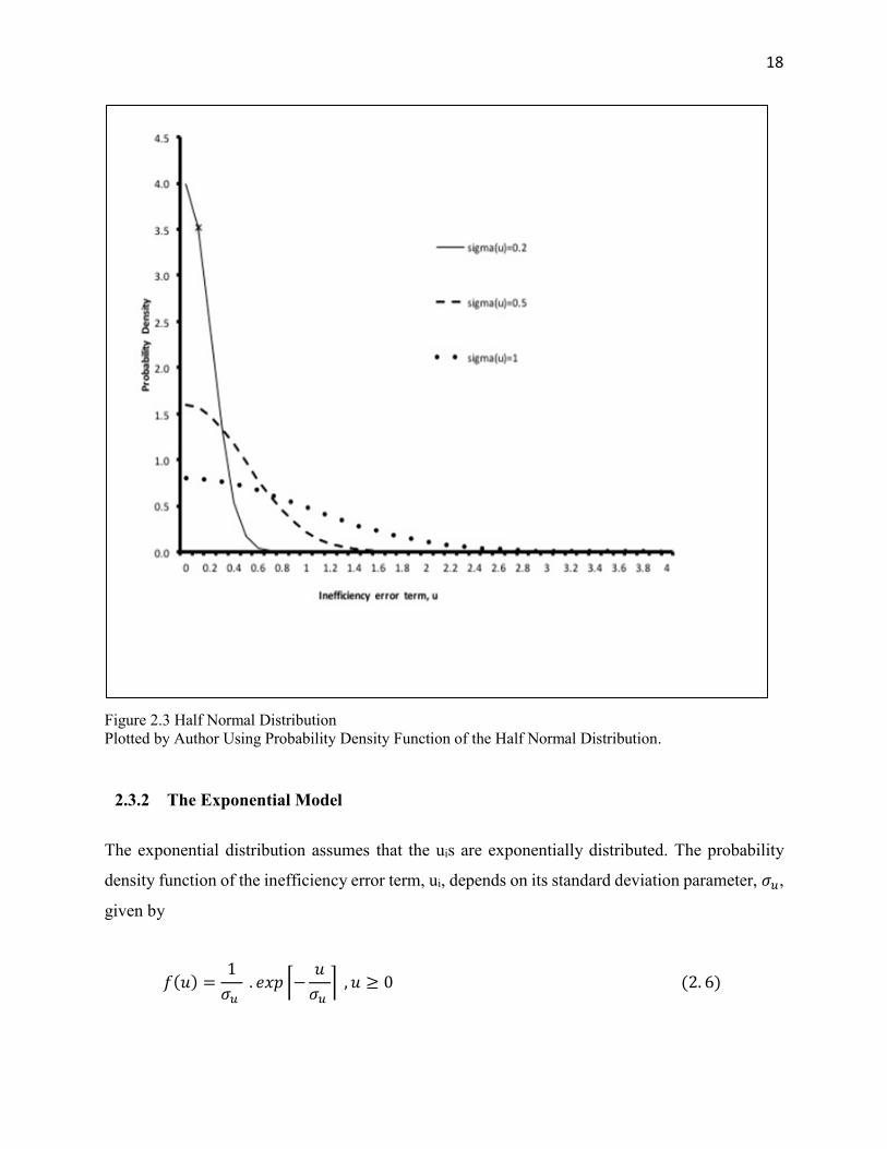
Figure 2.3 shows an illustration of the half-normal distribution for different values of the
standard deviation parameter, σu (=0.2, 0.5, and 1).
18
Figure 2.3 Half Normal Distribution
Plotted by Author Using Probability Density Function of the Half Normal Distribution.
2.3.2 The Exponential Model
The exponential distribution assumes that the uis are exponentially distributed. The probability
density function of the inefficiency error term, ui, depends on its standard deviation parameter, 𝜎𝑢,
given by
𝑓(𝑢) =1
𝜎𝑢 . 𝑒𝑥𝑝 ⌈−
𝑢
𝜎𝑢 ⌉ , 𝑢 ≥ 0 (2. 6)

19
Figure 2.4 shows the exponential distributions of various standard deviation values for the
inefficiency error term.
Figure 2.4 Exponential Distribution
Source: Plotted by Author Using Probability Density Function of the Exponential Distribution.

20
2.3.3 Truncated Normal Distribution Model
The half-normal model can be generalized by allowing the inefficiency error term, u, to follow a
truncated normal distribution. This is done by allowing the normal distribution, truncated below
at zero, to have a non-zero mode (Kumbhakar and Lovell 2003). Thus, an additional parameter, μ,
which is the mean of the truncated normal distribution is introduced. The truncated normal
distribution was formulated by Stevenson (1980) and makes the following distributional
assumptions.
i) ui ~ iid 𝑁+(𝜇, 𝜎𝑢2)
ii) Both ui and vi are independently distributed of each other, and of the explanatory
variables.
The truncated normal distribution, unlike the previous distributions, depends on two parameters,
𝜎𝑢 and μ. The density function is given as
𝑓(𝑢) =1
√2𝜋𝜎𝑢𝛷(−𝜇𝜎𝑢
). 𝑒𝑥𝑝 [−
(𝑢 − 𝜇)2
2𝜎𝑢2
] , 𝑢 ≥ 0 (2. 7)
where 𝜇 is the mean of the normal distribution truncated below at zero; Φ is the standard normal
cumulative distribution function. If 𝜇 is set to zero, the density function collapses to the half-
normal density function (i.e., when 𝜎𝑢 = 0.2). Figure 2.5 shows two truncated normal distributions
for two values of 𝜇 (i.e., μ=0 and μ=0.5) when 𝜎𝑢 is set to unity in both cases.
The estimation process with any of the above distributional assumptions involves setting
up a log-likelihood function which is maximized with respect to the parameters of the stochastic
frontier model to obtain ML estimates for 𝛽, 𝜎𝑢 2 and 𝜎𝑣
2 . Point estimates of the inefficiency error
term can then be predicted using the mean of the conditional distribution of u given 휀. Firm specific
TE can be obtained using the Battese and Coelli (1988) predictor given as

21
𝑇𝐸𝑖 = 𝐸(𝑒𝑥𝑝{−𝑢𝑖}|휀𝑖) (2. 8)
Figure 2.5 Truncated Normal Distribution
Source: Plotted by Author Using Probability Density Function of the Truncated Normal Distribution

22
2.3.4 The Choice of Distribution
Computational and theoretical considerations usually influence the choice of a distributional
assumption. The mean efficiency of a sample of producers is sensitive to the distributional
assumption of the one-sided error term, u and different distributional assumptions produce
different results regarding TE estimates. However, if a sample of producers are ranked on the
basis of the estimated technical efficiencies of the various distributions, these rankings tend to be
“quite robust” (Coelli et al. 2005 p.252) to the choice of distributional assumption (Kumbhakar
and Lovell 2003). For instance, Yane and Berg (2013) investigated the sensitivity of efficiency
rankings to the various distributional assumptions using Japanese water utilities data fit to Translog
stochastic production frontier models and found that the efficiency rankings were quite consistent
both under homoscedastic and heteroscedastic stochastic frontier models.
Also, Rossi and Canay (2001) investigated whether or not the choice of the half-normal or
exponential distributions matters in efficiency studies. Using public utilities data, they found that
the exponential distribution is associated with a larger number of efficient firms than the half-
normal distribution. However, the study found robustness regarding the efficiency rankings
between the two distributions.
According to Coelli et al. (2005), some researchers avoid the choice of the half-normal and
exponential distributions because both distributions assume that the inefficiency error term has a
mode at zero making it more likely that estimated inefficiency effects will be near zero and the
predicted TE in the neighborhood of one. However, the choice of more flexible distributions comes
at a computational cost due to the number of parameters that must be estimated. For instance, the
truncated normal distribution due to Stevenson (1980) beneficially relaxes the zero assumption for
the mode or mean of the inefficiency error term. This, however, according to Greene (2008), has
the disadvantage of inflating the standard errors of the parameter estimates and frequently inhibits
the convergence of iterations. Baten and Hossain (2014) estimated a stochastic frontier model
using rice production panel data from Bangladesh and assumed both half-normal and truncated
normal distributions. By comparing the performance of stochastic frontier models under the two

23
distributions through the method of likelihood ratio test, they found the half-normal distribution
model preferable to the truncated normal model with regards to the technical inefficiency effects.
In summary, the half-normal and truncated normal distributions are quite closely related to
each other since one is nested in the other. The truncated normal distribution is obtained by
truncating the normal distribution at zero and allowing the inefficiency error term to have a non-
zero mean or mode. If the mean or mode of the truncated normal distribution is set to zero, the
model collapses to the half-normal distribution. In this study, I only consider the truncated normal
distribution.
2.4 Panel Data Models
Data availability is key for SFA. According to Schmidt and Sickles (1984), cross-sectional
stochastic frontier models are associated with three serious problems. First, model estimation and
separation of technical inefficiency from statistical noise require strong distributional assumptions,
and it is not clear how robust the results are to these assumptions. Second, it may not be correct
to assume that the inefficiency component is independent of the regressors. This assumption is
particularly problematic if the firm knows its level of technical inefficiency which can affect its
input choice. Third, although the composite error term can be consistently estimated, the
estimation of technical inefficiency by the JLMS technique is not consistent because the variance
of the distribution of the technical inefficiency parameter does not approach zero as the number of
firms approaches infinity.
The above limitations can be avoided if one has access to panel data. First, the estimated
technical inefficiency will be consistent as the number of observations (T) of each firm approaches
infinity. Second, with panel data, one does not need to make the strong distributional assumptions
made under cross-sectional models. Third, access to panel data enables one to ignore the
assumption that the inefficiency error term is uncorrelated with the regressors (Schmidt and Sickles
1984). For this analysis, the data has a panel structure. The panel structure is provided by the
existence of multiple heterogeneous farm subplots across each household.

24
There are two methods for estimating stochastic frontier models with panel data:
distribution-free approaches and ML methods. Both time-varying and time-invariant models are
available within each of these approaches.
The distribution-free methods are desirable as they do not require distributional
assumptions for the estimation of inefficiency. Despite this desirable attribute, it is possible to
make distributional assumptions on the error terms and estimate panel stochastic frontier models
using ML methods. The ML methods can be more efficient given appropriate distributional
assumptions (Kumbhakar 1990). In this section, I briefly discuss time-varying and time-invariant
panel data models using ML methods.
Using the half-normal case, assume sample data on I producers, i=1, …, I; for T time
periods, t=1, …, T. The general form of a stochastic production frontier with the assumption of
time-varying technical inefficiency can be written as follows
𝑌𝑖𝑡 = 𝑓(𝑋𝑖𝑡 ; 𝛽)𝑒𝑥𝑝 (𝑣𝑖𝑡 − 𝑢𝑖𝑡), (2. 9)
where vit ~N (0, σv2) and uit ~N+(μ, σu
2 ). The variables have already been defined and the
inefficiency error term is allowed to change with time. More specifically, uit = ui. Gt, where Gt is
a function of time. For the error terms, let the assumptions for the truncated normal distribution
apply. The estimation process involves setting up a log-likelihood function which is maximized
with respect to the parameters to obtain ML estimates for β, Gt, σu 2 and σv
2 . Point estimates of the
inefficiency error term can be obtained using the mean of the conditional distribution of u given 휀.
Firm specific TE can then be obtained using
𝑇𝐸𝑖𝑡 = 𝐸(𝑒𝑥𝑝{−𝑢𝑖𝑡}|휀𝑖𝑡). (2. 10)
A number of time-varying models have been considered and estimated in the efficiency
literature. Battese and Coelli (1992) considered a decay model in which 𝑢𝑖𝑡 = 𝑢𝑖 . 𝐺𝑡, and 𝐺(𝑡) =
𝑒𝑥𝑝{−𝛾(𝑡 − 𝑇)}, where ui is assumed to follow a truncated normal distribution with non-zero

25
mean and constant variance, and 𝛾 governs the temporal pattern of inefficiency. They applied this
model to data from paddy farm ers in an Indian village. Kumbhakar (1990), on the other hand,
considered a similar but flexible model where 𝐺(𝑡) was specified as 𝐺(𝑡) = 𝑒𝑥𝑝[1 +
𝑒𝑥𝑝{𝛾1𝑡 + 𝛾2𝑡2}]−1 and 𝛾1 and 𝛾2 govern the temporal pattern of inefficiency. The second
parameter, 𝛾2 accounts for the possibility of a quadratic behaviour in inefficiency over time. Unlike
Battese and Coelli (1992), the Kumbhakar (1990) model assumes that the inefficiency error term
follows a half-normal distribution.
For the time invariant ML case, the equation is written as
𝑌𝑖𝑡 = 𝑓(𝑋𝑖𝑡 ; 𝛽) 𝑒𝑥𝑝(𝑣𝑖𝑡 − 𝑢𝑖), (2. 11)
where 𝑣𝑖𝑡 ~𝑁 (0, 𝜎𝑣2) and ui ~N+(μ, σu
2 ). The inefficiency error term is time independent unlike
in the previous case, however, the noise term is time dependent. A log likelihood function is set
up and maximized with respect to the parameters above to obtain consistent estimates for
𝛽, 𝜎𝑣2, and 𝜎𝑢
2 . The TE estimates can be obtained by using
𝑇𝐸𝑖 = 𝐸(𝑒𝑥𝑝{−𝑢𝑖}|휀𝑖𝑡). (2. 12)
Battese and Coelli (1988) assumed a truncated normal distribution for the inefficiency error
term and defined a stochastic production function for panel data for the Australian dairy sector. A
similar model was proposed by Kumbhakar (1987) under the assumption of profit-maximizing
behaviour of firms.
In this study, the structure of the available data has made it necessary to fit a panel data
model. Specifically, the panel data model of Battese and Coelli (1995) that allows for technical
change and time varying inefficiency is used. However, the available data do not vary across time
for each cross section; instead, there are multiple heterogeneous subplots within each household
making the data to have a panel structure that is different from traditional panel data (cross-
sectional time series). The time varying model would mean efficiency can differ between subplots

26
for a given household. More information about the characteristics of the data is provided in the
next chapter.
2.5 Determinants of (In)efficiency
Most production frontier studies not only estimate efficiency but also investigate factors that
positively or negatively impact efficiency. Exogenous determinants of efficiency are particularly
important for drawing policy conclusions. Public sector entities trying to increase the productivity
of firms particularly in agriculture not only need to assess efficiency but also identify sources of
inefficiency for the development of strategies and innovations to reduce these inefficiencies
(Sherlund et al. 2002). Thus, there is a need to establish a relationship between the measured
(in)efficiency and exogenous variables believed to affect efficiency.
Previous studies (Pitt and Lee 1981; Kalirajan 1981) have followed a two-stage estimation
method to investigate factors influencing technical inefficiency. The first stage involves estimating
the specified stochastic production frontier model and obtaining observation-specific inefficiency
measures. The inefficiency index is then regressed on a vector, Zi, of explanatory variables, in the
second stage. Kumbhakar et al. (1991) identified two problems with this approach. First, technical
inefficiency could be correlated with the production function inputs resulting in inconsistent
estimates of the ML parameters and inefficiency estimates. Second, the one-sidedness of the
technical inefficiency error term might make the Ordinary Least Square (OLS) results in the second
stage inappropriate. Also, if the Xis and Zis are correlated, the stochastic frontier model parameters
estimated in the first stage are biased due to misspecification (Wang and Schmidt 2002). Wang
and Schmidt (2002) further showed that even if the Xis and Zis are uncorrelated, the inefficiency
estimates in the first stage will be statistically under-dispersed making the results of the second
stage OLS biased. Their study uses a Monte Carlo experiment that shows the severity of the bias
caused by the two-stage estimation.
Given the above statistical limitations of the two-step estimation, a single-stage estimation
procedure was first proposed by Kumbhakar et al. (1991), followed by Reifschneider and
Stevenson (1991), Huang and Liu (1994), Battese and Coelli (1995), and Wang (2002).

27
The single-stage procedure involves parameterizing the distribution of the inefficiency
error term as a function of exogenous determinants, Zis. For the truncated normal distribution, the
mean of the distribution of the pre-truncated, i, is parameterized as a linear function of the
exogenous determinants. The equation for the inefficiency effects model with a truncated normal
distribution becomes
𝜇𝑖 = 𝑍𝑖′𝛿, 𝜇𝑖 ≥ 0. (2. 13)
2.6 Efficiency Studies in East Africa
This section reviews some of the existing efficiency literature in East African countries. The
efficiency literature in Eastern Africa is growing, and studies mostly focus on the agricultural
sector. Some East African studies applied SFA while others used DEA. Also, some studies
estimated inefficiency effect models to examine factors such as new technologies and socio-
economic variables that affect efficiency. In this review, apart from focussing only on efficiency
studies done on smallholder farmers, which this study examines, I also consider previous
efficiency studies that used data from commercial farmers in order to get a grasp of the nature of
agricultural efficiency in the region. Smallholder farmers in the area operate on small plots of land
(usually less than 0.5 hectares) and mainly grow subsistence crops and small amounts of cash
crops. The smallholder production system is characterized by use of simple traditional farming
tools, high reliance on family labour, low yields, and low technology adoption. Commercial
farmers, on the other hand, often operate large farms usually spanning hundreds of hectares and
mainly produce crops and animal products for sale to make profits. A summary of the selected
empirical studies is presented in Table 2.1
Kibaara (2005) used the single-stage stochastic frontier approach to estimate the TE of
maize production in Kenya using smallholder rural household data collected during the 2003/2004
main harvesting season by Tegemeo Institute of Agricultural Policy and Development. The study
also investigates the influence of socio-economic characteristics and management practices on the

28
TE of farmers. The study found mean TE of 49% with a range of 8-98%. Farmers who planted
hybrid maize varieties were found to be more efficient than those using local maize varieties. In
fact, use of a hybrid maize variety increased the mean TE by 36%. In addition, mono-cropped
maize farms were found to be more technically efficient than intercropped farms.
Alene and Zeller (2005) studied TE and technology adoption among Ethiopian farmers
growing maize, wheat and barley using a multi-output framework and compared parametric and
non-parametric distance functions for the adopters of improved technologies for cereal production
such as improved varieties and mineral fertilizers. They used stochastic distance functions for the
parametric approach and DEA for the non-parametric approach. The results from both methods
indicated considerable inefficiencies among the farmers. The study, however, found that the
estimates from the parametric distance functions (PDF) were less sensitive to outliers and hence
more robust than those from the DEA approach. Based on the PDF approach, the study found that
the adopters of these improved technologies had an average TE of 79% with a range of 28-100%.
A study by Chepng’etich (2013) used DEA to investigate the TE of sorghum farmers in
Machakos and Makindu districts in Kenya. The study found mean TE of 41% with a range of 1.5-
100%. The study further used Tobit regression analysis to determine the influence of socio-
economic characteristics such as education, membership to associations, income, experience,
production advice; and the use of technologies such as manure, tillage, and improved sorghum
varieties on farmers’ TE . Among these variables, manure use, education, experience, membership
in associations, and production advice were found to significantly increase TE. Use of improved
sorghum varieties did not have a significant effect on TE.
Mutoka et al. (2014) investigated the implications of Sustainable Land Management
practices (SLM) for resource use efficiency and farm diversity in the Western Highlands of Kenya.
Their study used SFA to measure the economic efficiency of 236 surveyed households, primarily
growing maize and beans. At the same time, the study examined the impact of Soil and Water
Conservation measures (SWC) on farmers’ resource use efficiency. They found mean economic
efficiency of 40% indicating under-utilization of land resources for agricultural use. Also, the study
found a positive impact of SWC measures on farmers efficiency.
29
Kalibwani et al. (2014) used nationally representative 2005-2010 panel data set from
Uganda to examine the performance of the agricultural sector in different regions of the country.
They used stochastic frontier model to measure TE across the regions. Their estimation follows
the model of Batesse and Coelli (1995). In addition to socio-economic characteristics, they also
investigated the effect of improved crop varieties on the efficiency of farmers. Overall mean TE
was found to be 85% with a range of 3.7-100%. The study found significant variation in mean
technical efficiency among the different regions studied. Age, gender, and education were found
to have significant affects on TE, whereas farmers’ adoption of improved crop varieties was
found to have no significant effect on TE.
Lemba et al. (2012) used DEA to compare the TE of five groups of farmers participating
in different farm intervention programs aimed at increasing productivity of the dry land farms in
Makueni, Kenya. The intervention types were: Improving access to water supply and extension
services provided by Danish Technical Cooperation in collaboration with the Kenyan government;
development and dissemination of drought resistant crop varieties provided through the
International Crops Research Institute for the Semi-Arid Tropics Project; improved farm
production resources provided through the Community Based Nutritional Program Project;
building the financial resource base of rural communities through savings and credit by village
banks; and access to irrigation provided by Israeli Technical Cooperation. For the full sample, the
study found mean TE of about 16% assuming constant returns to scale (CRS) and 22% assuming
variable returns to scale (VRS). About 70% of the farmers had a TE in the range 0-20%, and a
very small percentage of the farms (3.2%) were fully technically efficient under the constant
returns to scale TE measures. Among the five interventions, irrigation intervention was found to
be most effective in increasing farmers’ TE.
Mburu et al. (2014) estimated a stochastic frontier production model to examine the effect
of farm size on the technical, allocative and economic efficiency of a sample of 130 small and
large scale wheat farmers in Nakuru, Kenya. The study found mean technical, allocative and
economic efficiencies of 85%, 96%, and 84% respectively for small-scale farmers; and 91%, 94%
and 88% respectively for large scale farmers The closeness of the mean efficiencies implies that

30
both small and large scale farmers are relatively equally efficient at wheat production. Farm size
was found to have a significant effect only on allocative efficiency, and no impact on technical
and economic efficiency.
Mussaa et al. (2011) used DEA to estimate a production frontier function for a sample of
700 smallholder farmers in Ethiopia’s central highland districts. The objective of their study was
to measure resource use efficiency and examine factors such as family size, farming experience
and membership to associations that influence the productive efficiency of teff, chickpea, and
wheat. The study found mean technical, allocative and economic efficiency measures of 79%,
43%, and 31% respectively. The study found that age, family size, experience, distance to nearest
market, access to credit and land size significantly affect farmer TE. Membership of households
in associations was also found to increase economic efficiency.
Ngeno et al. (2012) used both SFA and DEA to measure the TE of a sample of 540
randomly selected commercial maize farmers in Uasin Gishu district of the Rift Valley province
in Kenya. The study categorized farmers into small, medium and large-scale. The results indicate
an overall mean TE of 85%. Regarding the three categories, the study showed a mean TE of 80,
83 and 95% for small, medium and large-scale farmers. Also, A study by Oduol et al. (2006) used
the DEA approach to examine the effect of farm size on the technical, allocative and scale
efficiency of smallholder farmers in the Embu district of Kenya. The study found overall mean
TE, scale efficiency and AE of 54%, 79% and 77% respectively. The study also found that large
and medium farms tend to have higher productive efficiency compared to small farms.
In summary, the studies above indicate that East African agricultural production is
associated with significant technical inefficiencies, with mean TE ranging from 16-89%. The
outcome of these studies seems contrary to the previously held view that farmers in the developing
world are efficient in their allocation of production resources. This view dates back to the well-
known “poor but efficient” hypothesis of Schultz (1964). Schultz argued that farmers in the
developing world are resource poor, thus operating below their potentials. However, the argument
goes, these farmers given enough time to learn about the production process, become efficient in
their allocation of resources and produce on the production frontier. Schultz advocated for policies

31
geared towards shifting the production frontiers of smallholder farmers through technology
adoption and use of more productive inputs. This concept later guided the Green Revolution and
much of recent research aimed at enhancing crop production technologies in the developing world
(Sherlund et al. 2002). Despite this hypothesis, empirical evidence shows that farming in the
developing world, particularly, smallholder farming, is associated with serious technical
inefficiencies and hence the emergence of studies recommending policies such as extension work,
farmer education, land reforms and so on; that can help farmers reallocate scarce resources to
improve their efficiencies (Sherlund et al. 2002).
Furthermore, none of the studies reviewed account for the influence of environmental and
geographical factors such as soil quality in the estimated production frontiers. Generally, few
studies in the stochastic production frontier literature account for inter-farm environmental and
geographic heterogeneity possibly due to data limitations. Sherlund et al. (2002) show that failing
to control for heterogeneity due to environmental factors can lead to omitted variable bias. They
support this claim with an analysis of rice data from Ivory Coast, and the results show a significant
difference in mean TE when environmental factors such as rainfall, location, and soil quality are
included in the model. For instance, they find mean TE of about 77% with environmental variables
compared to about 36% without environmental variables for the same data. More specifically,
failure to account for measures of soil capital in production functions could result in omitted
variable bias because farmer’s choice of agricultural inputs depends on not only on economic
conditions such as availability of labour and fertilizer but also on the quality and condition of the
soil (Ekbom and Sterner 2008). For this study, data on environmental factors are available.

32
Table 2.1 Summary of Selected Efficiency Studies in East Africa
Study Sample Crop(s) Method* Mean TE (%) Determinants of TE
Kibaara(2005) 2017 Maize SFA 49 Hybrid Maize variety, Tractor use, & education
Alene and Zeller (2005) 53 Maize, Wheat & Barley PDF 79
Chepng’ etich (2013) 143 Sorghum DEA 41 Land Size, Manure, Household Size, experience, memberships to
associations, hired labour, Production advice
Kalibwani, Mutenyo & Kato (2014) 364 Various Crops SFA 89 Age, Gender, Year, & Education
Lemba et al. (2012) 191 Various Crops DEA 16 – CRS
22 - VRS
Mburu, Ackello-Oguta & Mulwa
(2014)**
130 Wheat SFA 88 Education, Distance to extension advice, Farm Size
Mussaa et al. (2011) 700 teff, Wheat & Chickpea DEA 79 Membership to Associations, Market Distance, Access to credit, Land
Size, Age , Family Size, & Experience
Ngeno et al. (2012)** 540 Maize SFA & DEA 85
* SFA = Stochastic Frontier Analysis; PDF= Parametric Distance Function; DEA= Data Envelopment Analysis.
**These studies used data on commercial farmers.

33
2.7 Technology Adoption and Productivity
This short section illustrates the technical effect of new technology on productivity. As mentioned
earlier, technical change is realized when a firm’s production frontier is shifted outward and more
output is produced without changing the level of inputs. Figure 2.6 illustrates the effect of new
technology on productivity. The vertical axis shows output while the horizontal axis shows inputs.
Initially, the farmer’s production frontier is given by F0, and supposing that the farmer is
fully technically efficient at the initial level of technology, he operates at output level of 𝑌0. What
happens when the farmer adopts a new technology such as an improved seed variety? The adopted
technology shifts the production frontier outward, and the new production frontier curve is now
given by F1.Given this new technology, the new production point will be determined by the effect
of the new technology on the farmer’s TE6. If the farmer continues to be fully technically efficient
at the new technology, then he will produce at Y1 realizing an increase in productivity.
If the new technology decreases the farmer’s TE, the change in productivity will depend
on the new production point Y1 in relation to the old production point, Y0. If the new point is
above Y0, the farmer’s productivity has increased even if he is not producing on the new output
frontier (despite the decline in TE) because the technology effect dominates. On the other hand, if
the new production point is below Y0, the decrease in TE is so high that productivity decreases.
6 A relationship between technical efficiency change and technological change is that a change in
technology can also bring about an impact on technical efficiency and the effect can either be
negative or positive (Medhin and Köhlin 2011).

34
Figure 2.6 Technology Adoption and Productivity

35
2.8 Soil Organic Carbon and Implications for Productivity
Most smallholder farmers in the Sub-Saharan Africa live on marginal7 farmlands characterized by
severely depleted soils that hinder them from attaining the full potential of the production resources
available to them. The collapse of traditional farming methods such as long-duration fallows, low
rural agricultural development, and population pressures all contribute to the continuous decline
in soil fertility (Berazneva et al. 2014; Marenya and Barrett 2009). As the region’s population
grows, more lands are being cleared for settlements and farming leading to excessive cultivation
and deforestation, a decline in soil fertility, and significant losses of soil organic matter in the form
of CO2 and NO2 gases into the atmosphere. Loss of carbon stored in the soil, apart from having
adverse consequences for soil fertility, also adds to GHG emissions. Also, the response of these
depleted soils to farmer’s application of mineral fertilizers has often been very low, pushing
smallholder farmers to “cultivate marginal soils with marginal inputs, produce marginal yields,
and perpetuate marginal living and poverty” (Lal 2004 p.1626).
Marenya and Barrett (2009) argue that policies aimed at addressing degraded soils through
increased access to fertilizer benefits only wealthy farmers who cultivate fertile soils. Given that a
positive relationship exists between soil quality and wealth, this leads to “soil degradation poverty
traps” (2009 p.993) where only relatively affluent farmers who cultivate fertile soils have
incentives to invest in soil improving technologies such as fertilizers, thus achieving higher yields
while also sustaining pre-existing soil carbon stocks. Poor farmers, on the other hand, have no
incentive to invest in the replenishment of already depleted soils.
The management of soil resources and replenishment of soil nutrients is of utmost
importance in order to simultaneously tackle the biophysical causes of low economic development
and environmental degradation in SSA (Berazneva et al. 2014; Marenya and Barrett 2009). The
enhancement of soil quality through improvements in soil organic carbon has been seen to address
both food security and climate change challenges. The adoption of soil conservation practices
7 According to Kang et al. (2013), marginal lands are lands “characterized by low productivity
and reduced economic return or by severe limitations for agricultural use” (p.129). In economic
terms, these lands will tend to require large amounts of external inputs.

36
remains the most promising strategies to build up soil organic matter to enhance the long term
fertility and nutrient efficiency of soils, while at the same time sequestering carbon (Berazneva et
al. 2014; Lal 2006).
Carbon sequestration has both food security enhancement and climate change mitigation
benefits. Soil carbon pools can be increased by land management strategies such as no-till farming,
cover crops, legume intercropping, agroforestry, and manure applications. These practices must
be adopted at high rates and in recommended combinations in order to reverse soil degradation,
alleviate poverty levels and mitigate GHGs. There are few studies in the SSA that examine the
potential impacts of soil conservation practices on soil organic carbon for improved yields and
reduced GHGs. An 18-year experiment published by Kapkiyai et al. (1999) tested the effect of
three management practices (fertilizer application, cattle manure application and retention of
maize stover) on crop yield, soil organic matter and soil chemical properties for smallholder
farmers in Kibete, Kenya. The results showed that total crop yield for maize and beans ranged
from 1.4 t ha-1 yr-1 with maize residue retention to 6.0 t ha-1 yr-1 when all the three practices were
incorporated. The corresponding soil organic carbon content (depth of 15 cm) ranged from 23.6 t
ha-1 yr-1 with fertilizer application and residue removal to 28.7 t ha-1 yr-1 with mineral fertilization,
manure application and residue retention. Further, continued mineral fertilization and residue
removal led to an average soil organic matter loss of 0.56 t C ha-1 yr-1. In relation to this, the study
found that manure application and residue management reduced this loss by 49%.
In addition, a seven-year field experiment in the Gansu province of China, published by
Cong et al. (2015) examined the soil carbon (%C) and nitrogen (%N) contents of rotational
intercrop systems and ordinary crop rotations. The study found that soil organic C content in the
top 20 Centimeters was 4% ± 1% greater in intercropped fields than in monocropped fields. The
study further found that carbon sequestration rate in the intercropped fields was 0.184 ±
0.086 t C h−1 Yr−1 higher than in monocropped fields and that total root biomass in intercropped
fields was on average 23% higher than the average root biomass in monocropped fields. A note of
caution, however, is that leguminous crops also release significant amounts of NO2 into the
atmosphere, which may offset the carbon effect on overall GHG emission.

37
Soil carbon is not fixed over time, and its changes could be determined by the kind of
production practices undertaken by farmers. For instance, continued residue management coupled
with other soil conservation management practices has multiple benefits including increased soil
organic carbon stocks, carbon sequestration, nutrient recycling, improved soil properties, erosion
control and an increased use efficiency of other inputs (Lal 2008; Berazneva et al. 2014).
Soil carbon is a major factor of production. Apart from management decisions such labour
inputs, fertilizer application, and land allocation that directly affect agricultural productivity, soil
carbon management represents a significant factor in agricultural productivity. ‘Valuing the
environment as an input’ is an essential method to account for the contribution of the ecosystem
to productivity (Barbier 2007; Lal 2004). In fact, studies trying to examine the ecosystem value of
soil carbon tend to use the production function approach as a potential method for disentangling
the contribution of soil carbon and one way to this is by estimating the impact of soil carbon on
agricultural yields (Pascual et al. 2015). Thus, quantifying the marginal change in agricultural
yield due to a marginal change in soil carbon provides valuable information about the functional
relationship between soil carbon and agricultural production (Pascual et al. 2015). In this study,
soil carbon is treated as an environmental quasi-fixed factor of production (fixed within a period
but infrequently changing depending on previous levels and farming practices adopted).
The remainder of this section focusses on discussing a simple framework that emphasizes
the dynamic nature of soil carbon, and the effect of adopted practices such as residue management
and intercropping on agronomic productivity through their effects on soil carbon.
Suppose that a maize farmer is endowed with a piece of land of homogeneous quality. The
soil fertility state of the farmer’s land is characterized by a single soil quality indicator-soil carbon
content, denoted by Ct. The farmer grows maize on this piece of land by employing a range of land
use and management decisions. Focussing on residue management as a land use management
decision, let 𝜓𝑡 ∈ [0, 1] be the share of crop residues returned to land at the end of year t that
affects the stock of soil carbon in period t+1. Let the farmer’s maize production (Yt) at time t be a
function of a composite variable input, Xt, and soil carbon content, Ct. The equation of the
production function is given by

38
𝑌𝑡 = 𝑌(𝐶𝑡, 𝑋𝑡), (2. 14)
where Y(.) denotes a yield function. Further, let the change in soil carbon content in period t+1
depend on the previous soil carbon content and the residue management decision undertaken by
the farmer in the previous period. The carbon dynamics equation is given by
𝐶𝑡+1 − 𝐶𝑡 = 𝑓(𝐶𝑡, 𝜓𝑡), (2. 15)
where f(.) describes soil carbon dynamics. The equations show that given a starting level of soil
carbon, C0 > 0, land management decisions such as adoption of soil conservation practices have
an impact on the periodic changes in soil carbon which in turn affects agronomic productivity
(production per unit of land). An empirical study involving carbon dynamics needs access to
historical data on soil carbon. In this study, I only have access to one-period data on soil carbon
and other production variables. Carbon dynamicsare therefore not captured in the empirical work.
Soil carbon is treated as an input in the estimated production functions.
Despite the significant implications of soil carbon for productivity and climate change
mitigation, very few studies have used soil carbon as a factor in production functions. Berazneva
et al. (2014) used a bioeconomic model to investigate the impact of soil carbon management on
production by estimating, among other models, a quadratic maize production function with carbon
stock and nitrogen fertilizers as inputs. Their study found a significant effect of soil carbon stocks
on maize output. Marenya and Barrett (2009) estimated maize production function using soil
carbon as one of the factors of production. The aim of their study was to examine the
complementarity relationship between soil organic matter (SOM), fertilizer application and
profitability in soils with low SOM. Their study found that low SOM limits the response of yield
to fertilizer application. López (1997) examined the effect of village biomass as a factor of
agricultural production using a Cobb-Douglas production function and found a significant effect
of village level biomass on agricultural production.
39
3 . Empirical Methods
This chapter is divided into five main sections. Section 3.1 describes the site chosen for this study.
Section 3.2 discusses the data and gives descriptive and exploratory statistics. Section 3.3 outlines
SFA, introduces the model and assumptions and presents the econometric model specified for the
data. Section 3.4 describes technique of estimation, while Section 3.5 discusses the functional
forms used in the estimation.
3.1 Site Information
The site chosen for this study is Nyando, a CCAFS site in the Nyando district in Western Kenya.
The surveyed households live within the Nyando river basin of Lake Victoria. The Nyando river
basin covers an area of about 3587 KM2 with a population of 656,000 and a population density of
183 persons/KM2 as per the 1999 census (Swallow et al. 2009). The majority of the inhabitants
throughout the Basin are poor smallholder farmers who depend on rain-fed mixed agriculture for
their livelihoods. Smaller numbers of farmers practice irrigation farming in the lower area, large-
scale commercial sugarcane farming in the mid-altitude areas, and large scale tea production in the
upper altitudes (Swallow et al. 2009).
The Nyando river basin lies approximately between longitudes 34047” E and 35044” E, and
latitudes 0007” N and 0020” N. The area is characterized by a historical pattern of severe land
degradation and deforestation as human settlement and farming expanded along the basin with low
adoption of best land management practices (Raburu et al. 2012; Verchot et al. 2008). Land
degradation is made worse by frequent floods particularly in the low-lying areas, rendering 75%
of the plains unsuitable for farming (Raburu et al. 2012). The area is also characterized by severe
soil erosion. According to Swallow et al. (2009), severe gully erosion in the lower areas of the
basin is the most visible sign of land degradation in the basin, and land conversion and farming
degradation have increased the severity of soil erosion and sedimentation in the basin over the past
60-100 years.

40
The Nyando River basin is characterized by humid to sub-humid climates with annual
rainfall ranging from less than 1000 mm in areas near Lake Victoria to over 1600 mm in the
highland areas (Swallow et al. 2009). There are two rainy seasons. Short rains start between April
and May while long rains start between August and September (Waruru et al. 2003).The Western
Kenyan Integrated Management Project (WKIEMP) divides the Nyando River basin and its
inhabitants into three blocks namely Lower, Middle and Upper Nyando based on biophysical
features identified through satellite imagery and ground survey (Verchot et al. 2008). The Lower
Nyando is characterized by low elevation, moderate slopes, and unreliable rainfall that can sustain
mainly drought-resistant crops like sorghum and millet. The Middle Nyando is characterized by
higher elevation, steep slopes and less intermittent rains. The Upper Nyando is characterized by
large farms, higher elevation and steep slopes.
Swallow et al. (2009) show that large differences exists in per hectare value of agricultural
yield among the three blocks according to 1991 yield data. The lower altitude areas were
characterized by lower per hectare value of production of less than Ksh 5000, whereas in the mid-
altitude areas, the value of production was in the range of Ksh 5000-15000 per hectare. On the
other hand, the value of production in the high altitude areas ranged from Ksh 45-50,000 per
hectare.

41
Figure 3.1 Location Map of Nyando
Source: Raburu et al. (2012)
Figure 3.2 Map of Nyando River Basin Showing the Three Blocks.
Source: Verchot et al. (2008).

42
3.2 Data: Sources, Survey Design and Descriptive Statistics
The data used for this study come from three sources. The production data and household socio-
economic characteristics come from the Climate Change Agriculture and Food Security (CCAFS)
IMPACTlite data collected in 2012 through a survey done in 15 of CCAFS benchmark sites in 12
countries in Africa and South East Asia. Nyando is one of those sites. The Integrated Modelling
Platform for Mixed Animal Crop Systems (IMPACT) is a data collection tool that gathers detailed
information from smallholder farmers. In 2011, the International Livestock Research Institute
(ILRI) was commissioned by CCAFS with the task of simplifying IMPACT to enable collection
of household level data with enough detail to capture within-site variability on key livelihood
indicators, so that researchers from different disciplines could use for a range of analysis (Rufino
et al. 2012 ). This led to the modification of the IMPACT into IMPACTlite. In 2012, a survey
using the IMPACTlite tool was implemented in 15 of the CCAFS benchmark sites.
The IMPACTlite survey built on survey data that were available through CCAFS
household baseline survey carried out in 2010/2011. More specifically, the survey in Nyando
started with an analysis of satellite images, group, and individual interviews. Village lists were
developed and village boundaries marked in consultation with village elders. The selection of the
village lists was based on three production systems (consistent with the design of the earlier
Western Kenyan Integrated Management Project): maize-sorghum in Lower Nyando, sugarcane-
maize in Middle Nyando, and dairy-perennials-maize in Upper Nyando. The identification of the
production systems was based on the intensity of land use, land cover, and orientation of
production (Rufino et al. 2012). Eight villages were selected to represent the first production
system, and six villages were selected to represent each of the second and third production
systems. Ten households were randomly picked from each of the villages and 200 households
were surveyed.
The IMPACTlite data are detailed and capture information about subplot level crop
production, input and land usage, and socio-economic characteristics. The data were collected with
special concern for climate change and gender, capturing farmers’ subplot specific resource

43
allocation, crop and animal production, subplot gender ownership, and certain conservation
practices namely residue management and intercropping indicated at the subplot levels.
The IMPACTlite data were organized into data sets, each data set containing variables in
a specific category such as crop production or labour usage. Each of the categories is identified by
household, plot8 and subplot9 identifications. For this study, I merged the different categories
together by using the identifiers above. For each household’s plot, the survey recorded the data at
the subplot levels. For the purpose of this study, I focused on subplot level observations since the
subplot captures the different land use patterns taking place in a particular plot within a specific
period of time (Rufino et al. 2012). Accordingly, the survey asked farmers to state various farming
activities, crops grown, seed varieties used, and improved technologies adopted in a particular
subplot during a particular season of the year. Since each household has multiple subplots, the data
has a panel structure. The SFA analysis thus considers variation in production and TE between
sub-plots of the same farm, rather than between years on the same plot.
I obtained data for a total of 356 maize subplots from 183 of the 200 households surveyed.
This means that 91.5% of the households in Nyando cultivate maize among other crops. I dropped
32 subplots from 13 households whose yield was less than 10 kilograms10 and finally ended up
with 324 subplots from 170 households. These data were used for the analysis.
Extra data were obtained from different sources. Data on soil erosivity come from the
Reconnaissance Soil Survey collected at scale of 1:25,000 by Kenya Soil Survey (KSS) in 2003
8 Plot is defined as “land management unit whose dimensions do not change in time. It is a piece
of land owned, leased in or out, and can be fully cropped, kept fallow, used for grazing, forestry
or aquaculture”(Rufino et al. 2012) 9 Subplot is defined as “a sub-unit within a plot used to record differences in land use pattern in
space and/or in time. The purpose of using the sub-plot concept is to be able to describe framing
activities that may change in space or in time and to record labour and inputs demanding
activities, production and the use of crop residues” (Rufino et al. 2012 p.17). 10 These subplots had extremely low maize output and were dropped to mitigate the effect of
outliers on estimation. On the other hand, there were no subplots with extremely high output.
Although not as bad as DEA, SFA models are also sensitive to outliers. Outliers and extreme
values affect the ML method used to estimate SFA models (Song et al. 2015).

44
for Nyando, Kenya. Those data were provided by Joseph Sang, a lecturer at Jomo Kenyatta
University of Agriculture and Technology (JKUAT). Data on climate (precipitation and
evapotranspiration) is a digital climate surface sourced from USAID’s Office of Foreign Disaster
Assistance (OFDA) collected by USAID's Development Strategies for Fragile Lands project
(DESFIL) and was downloaded from the GIS services website of the International Livestock
Research Institute (ILRI). Data on soil organic carbon and household geographic coordinates were
sourced from ILRI through David Pelster, a research scientist and Carlos Quiros, agricultural
information systems specialist. All the three data (soil and climate variables) were in shapefiles. I
used ArcGIS 10.1 software to merge the climate, soil and IMPACTlite data using the geographic
coordinates of the surveyed households.
Table 3.1 describes the variables used in the study and provides summary statistics for each
of the variables. The yield variable shows harvested amount of maize grains in Kilograms obtained
from a specific subplot for a specific period in the year. Average subplot yield for maize was about
479 kilograms ranging from 12 Kg to about 8100 Kg per subplot. The standard deviation for maize
yield is greater than the mean indicating that the yield data points vary widely around the mean.
The labour variable is defined by total days of labour spent on a subplot and includes family
and hired labour. Average labour spent on the subplots was about six days, with a minimum of one
day and a maximum of 60 days. Land size is measured in hectares. The average subplot size
allocated to maize is about one hectare and ranges from 0.02 hectares to 7.5 hectares.
The seed variable represents the amount of money in Ksh spent on seeds used in a subplot.
The seed variable is reported in the data as the amount of seeds used for a particular crop, the type
of seed (local or improved variety) and market value in Ksh per Kilogram. I have chosen to use
the market value of seed to account for the possibility that local and improved seed varieties are
not equally productive. On average 4232 Ksh in seeds is spent on the subplots, and the amount
ranges from 37.5 to 375,000 Ksh.
The carbon variable is defined by the percentage amount of organic carbon in the soil (%
C). The average soil carbon content is 1.788% and ranges from 1.3% to 3% with standard deviation
45
of 0.553%. Soil erosivity refers to the susceptibility of soil to be eroded by rain, wind or surface
runoff (Zorn and Komac 2013). The susceptibility of the soil to erosion is mainly a function of the
slope of the landscape (Waruru et al. 2003). In the Nyando catchment area, erosion susceptibility
is generally high in the hilly and mountainous lands, while the plateau and plains have lower risk
(Waruru et al. 2003). According to the Kenya Soil Survey data from which this variable has been
obtained, erosion hazard was determined based on factors such as land form (mountains, hills,
plateau, upland, e.t.c), slope of the landscape, and soil properties such as soil cover or land use,
percentage amount of soil carbon, silt clay ratio, soil depth, level of exchangeable sodium, and
flocculation index11 (Waruru et al. 2003). Based on these factors, the erosion hazard of the Nyando
basin ranges from slight, moderate, high, severe, to very severe. The erosion hazard for the sample
of farmers for this study ranges from slight, moderate, high, to severe. An erosion index12 has been
constructed for these erosion hazard levels and ranges from one to four with one being slight and
four depicting severe erosion.
The P/EP variable is defined as precipitation/evapotranspiration obtained by dividing
annual precipitation by annual evapotranspiration. Evapotranspiration is the sum of evaporation
and plant transpiration. When P/PE is more than one, precipitation is higher than
evapotranspiration and more moisture is available for crops to grow. When the ratio is less than
one, evapotranspiration is greater than precipitation and the risk of drought could be higher and
more water is lost from plant crops through transpiration and evaporation. For the sample data,
average P/EP is 0.950 and ranges from 0.759 to 1.077.
The variables improved crop variety, residue management and legume intercropping are
dummies each denoting one if a specific practice was adopted on the subplot, zero otherwise. In
this study, the crop variety variable is defined by whether a household used an improved or a local
maize variety on a subplot. There are different maize varieties including the local varieties that the
farmers in Nyando have adopted on their subplots13. Residue management is defined by whether
after harvest crop residues have been left on the field or not. Intercropping is the growing of two
11 The degree in which individual soil particles are aggregated together. 12 1= Slight; 2 = Moderate; 3 = High; 4 = Severe 13 Some of the most common improved varieties adopted by households include: Hybrid, DH14,
DH04, KenyaSeed, 505, Yellow maize and H614

46
or more crop types in one field. In this study, the variable is defined by whether a household has
grown maize with beans in the same subplot or not. The average adoption rate of improved seed
varieties was found to be 81.8% which is relatively higher compared to residue management
(69.1%) and legume intercropping (2.07%).
The gender variable is defined by whether a subplot is owned by male or female and
represented by a dummy-one if a subplot is owned by male, zero otherwise. About 68% of the
subplots are owned by males. The distance variable refers to the distance of the subplot from the
homestead in meters. Average subplot distance is about 160 meters with a range of 0 to 5000
meters. The plough variable is defined by whether a household owns a plough or not and
represented by a dummy-one if a household owns a plough, zero otherwise. The sample data
shows that about 49% of the households own a plough. The radio variable is defined by the number
of radios the household owns. Average radio ownership per household is about 1 and ranges from
0 to 3 for the households. The adult variable is represented by the number of adults who are 18
years and above living in the household. On average, about three adults live in a household and
the range is from one to seven. The income variable represents average monthly off-farm income
in Kenyan Shillings. Households mentioned income from off-farm activities such as employment,
business, and remittances. Average household income for the sample ranges from 0 to 35000
Kenyan Shillings.
I present equality of means tests for maize yield under residue management, intercropping
and improved maize variety. The aim of these tests is to ascertain whether or not a significant
difference in mean yield exists between farmers who did or did not use these practices. The results
of the tests are presented in Table 3.2. The means test results reveal a significant statistical
difference in yields between users and non-users of each of the three practices. All the individual
tests reject (p-value <0.01) the null hypothesis of no difference in mean yield between users and
non-users of the practices. Intercropping shows the highest difference in mean yield among
adopters and non-adopters followed by variety and residue management.
Table 3.3 presents a correlation matrix for all of the variables used in the estimation of the
stochastic production frontier function. The computation of the correlation coefficients is aimed at

47
exploring the association between the output variable and the variables proposed as factors
responsible for variation in yield. The correlation coefficients of land, seeds, labour, carbon and
P/PE show significant (p-value <0.01) positive association with yield. A positive relationship
exists between yield and each of these variables. Land is most highly correlated (0.599) with yield
followed by labour (0.440), carbon (0.302) and seeds (0.297) in that order. The variety variable is
significantly correlated with yield with a correlation coefficient of 0.202. Also, there is a positive
relationship among some of the explanatory variables. Carbon is significantly correlated with
labour. Variety is significantly correlated with soil carbon, Erosivity and P/PE. Also, P/PE is
correlated with labour, land, carbon and erosivity. These correlations among the explanatory
variables could pose potential multicollinearity problems in the production function and stochastic
frontier models.
Having seen a positive and statistically significant relationship between yield and each of
the input variables, I am also interested in further exploring the pure association between yield and
each of the explanatory variables14 while controlling for the variation from other variables. This is
done by computing the partial correlation of yield with each of these inputs. Table 3.4 presents the
partial correlation coefficients. The results of the partial correlation coefficients show that land is
highly statistically correlated (0.496) with yield even after controlling for the variation in other
variables. The seed variable becomes second (0.320) once the variations from the other inputs are
partialled out followed by labour (0.270) and carbon (0.193) in that order. P/PE and Variety are
also correlated with yield with coefficients 0.095 and 0.101 respectively. The results of the
correlations between yield and the inputs labour, land, seeds and soil carbon support the technical
relationship between the inputs and yield.
14 Only those variables significantly correlated with maize yield are used in computing the partial
correlations.
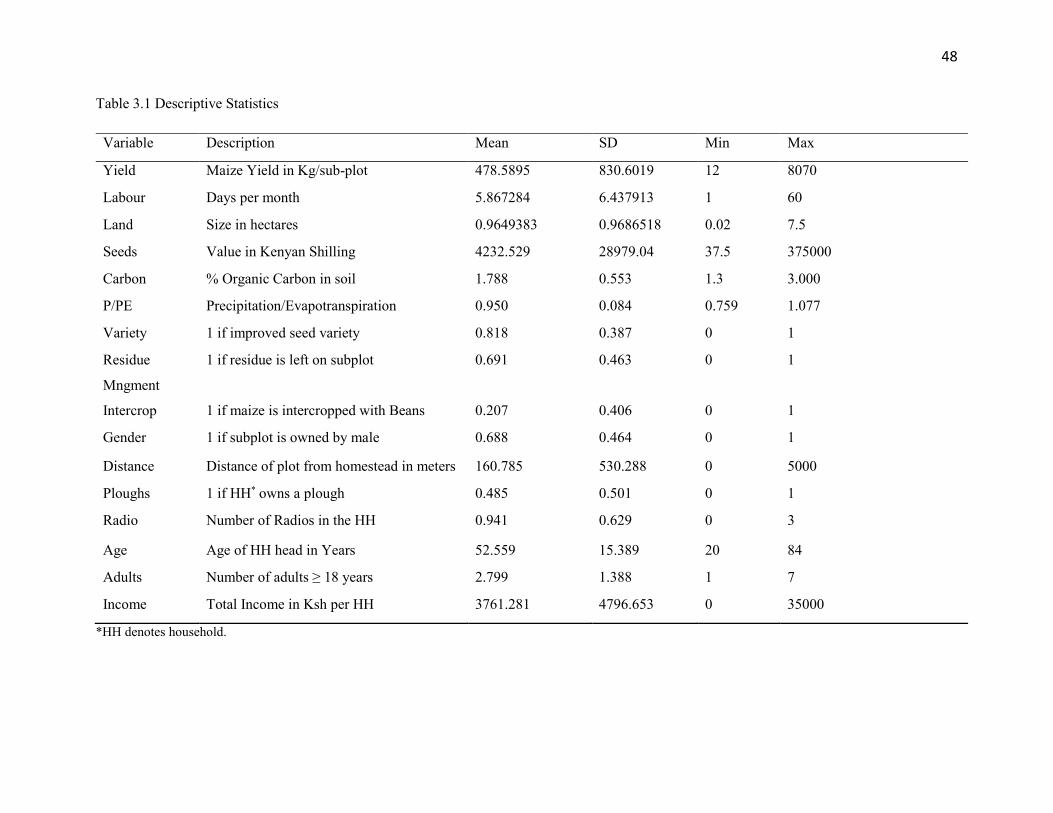
48
Table 3.1 Descriptive Statistics
Variable Description Mean SD Min Max
Yield Maize Yield in Kg/sub-plot 478.5895 830.6019 12 8070
Labour Days per month 5.867284 6.437913 1 60
Land Size in hectares 0.9649383 0.9686518 0.02 7.5
Seeds Value in Kenyan Shilling 4232.529 28979.04 37.5 375000
Carbon % Organic Carbon in soil 1.788 0.553 1.3 3.000
P/PE Precipitation/Evapotranspiration 0.950 0.084 0.759 1.077
Variety 1 if improved seed variety 0.818 0.387 0 1
Residue
Mngment
1 if residue is left on subplot 0.691 0.463 0 1
Intercrop 1 if maize is intercropped with Beans 0.207 0.406 0 1
Gender 1 if subplot is owned by male 0.688 0.464 0 1
Distance Distance of plot from homestead in meters 160.785 530.288 0 5000
Ploughs 1 if HH* owns a plough 0.485 0.501 0 1
Radio Number of Radios in the HH 0.941 0.629 0 3
Age Age of HH head in Years 52.559 15.389 20 84
Adults Number of adults ≥ 18 years 2.799 1.388 1 7
Income Total Income in Ksh per HH 3761.281 4796.653 0 35000
*HH denotes household.

49
Table 3.2 Descriptive Statistics and Results of T-tests of Maize Yield by Management Practice
Note: *** indicates statistically significant at 1%.
Group
Adopters Non-Adopters
Practice Mean SD N Mean SD n t diff
Residue Mngment 574.585 913.330 224 263.560 551.666 100 3.156*** -311.025
Intercropping 1009.925 1171.858 67 340.070 650.590 257 -6.212*** -669.855
Variety 557.668 897.569 265 123.407 134.596 59 3.703*** -434.261

50
Table 3.3 Correlation Matrix for the Variables Used in the Stochastic Production Function
Variable Yield Labour Seeds Land Carbon Erosivity P/PE Variety
Yield 1.000
Labour 0.440*** 1.000
Seeds 0.297*** 0.019 1.000
Land 0.599*** 0.389*** 0.164 1.000
Carbon 0.302*** 0.175*** -0.090 0.083 1.000
Erosivity -0.003 0.005 0.020 -0.030 0.183*** 1.000
P/PE 0.345*** 0.182*** -0.022 0.201*** 0.631*** 0.256*** 1.000
Variety 0.202* 0.076 0.022 0.085 0.236* 0.164* 0.318* 1
Note: *** indicates statistically significant at 1%
Table 3.4 Partial Correlations of the Variables Significantly Correlated with Maize Yield
Variable Partial Correlation Significance Level
Labour 0.270 ***
Seeds 0.320 ***
Land 0.496 ***
Carbon 0.193 ***
P/PE 0.095 *
Variety 0.101 *
Note: ***, **, and * represent significance at 1%, 5% and 10% respectively.

51
3.3 Stochastic Frontier Analysis
As discussed in Chapter two, the measurement of subplot level TE of Nyando maize growers
involves the estimation of a stochastic production frontier model with two error terms, one that
accounts for statistical noise and another to account for deviations from the production frontier
due to inefficiency. The stochastic production frontier function takes the following general form
𝑌𝑖𝑗 = 𝑓(𝑋𝑖𝑗, 𝛽) 𝑒𝑥𝑝(𝑣𝑖𝑗 − 𝑢𝑖𝑗), (3. 1)
where for each of the jth subplot of the ith household, Yij is output; Xij is a 1 by K vector of inputs
and other explanatory variables; 𝛽 denotes a k by 1 vector of unknown parameters to be estimated.
SFA is used to separate the two error terms mentioned above into statistical noise and inefficiency
components. The resulting inefficiency term can be used to construct measures of TE, and the
formula is given as
𝑇𝐸𝑖𝑗 =𝑌𝑖𝑗
𝑌𝑖𝑗∗ =
𝑓(𝑋𝑖𝑗 ; 𝛽) 𝑒𝑥𝑝(𝑣𝑖𝑗 − 𝑢𝑖𝑗)
𝑓(𝑋𝑖𝑗 ; 𝛽) 𝑒𝑥𝑝(𝑣𝑖𝑗)= 𝑒𝑥𝑝(− 𝑢𝑖𝑗). (3. 2)
As shown by the formula in 3.2, TE is a ratio of observed output to the corresponding
frontier output estimated using SFA. The measures of TE lie between zero and one, where a
measure of zero implies complete technical inefficiency and one implies full TE.
3.3.1 The Model and Assumptions
This study employs the inefficiency effects model of Battese and Coelli (1995). Given the general
specification of the stochastic production frontier function model given in equation 3.1 above, the
following distributional assumptions are made in reference to the error structures.
vij ~ N(0, σv2),

52
𝑢𝑖𝑗 ~ 𝑁+(𝛧𝑖𝑗𝛿, 𝜎𝑢2).
The vijs are independently and identically distributed with mean and variance as outlined above;
the uijs are non-negative random variables associated with the technical inefficiency of production,
distributed iid , and obtained by truncation of the normal distribution at zero with mean Ζijδ and
variance σu2; the Ζij is a 1xm vector of explanatory variables that are hypothesized to affect the
technical inefficiency of production; and 𝛿 is a mx1 vector of unknown coefficients on the factors
affecting inefficiency. The Zij includes both subplot level and household level characteristics and
technologies that affect technical inefficiency. Additionally, uij and vij are independently
distributed.
The technical inefficiency effect model is specified as follows.
𝑢𝑖𝑗 = 𝛧𝑖𝑗𝛿 + 𝜔𝑖𝑗, 𝑢𝑖𝑗 ≥ 0, (3. 3)
where ωij is a random variable with mean of zero and variance of 𝜎2. Battese and Coelli (1995)
propose the method of ML to simultaneously estimate the parameters of the stochastic frontier and
technical inefficiency effects models.
The Battese and Coelli (1995) model assumes a truncated normal distribution for the
inefficiency error term and a normal distribution for the random error term. The probability density
functions for both error terms and the log-likelihood function of the model can be found in Battese
and Coelli (1993). The log-likelihood function is expressed in terms of the variance parameters.
𝜎2 = 𝜎𝑣2 + 𝜎𝑢,
2 (3. 4)
and
𝛾 = 𝜎𝑢
2
𝜎𝑣2 + 𝜎𝑢
2, (3. 5)

53
where ε = v − u and γ is the ratio of the variance of the inefficiency error term to the variance of
the whole error term. The log-likelihood function is maximized with respect to the parameters,
β, δ, σε, and γ to obtain their ML estimates.
The technical inefficiency component of the combined error term cannot be observed and
therefore must be predicted from the conditional distribution of u given ε. The subplot level TE
is defined as
𝑇𝐸𝑖𝑗 = 𝑒𝑥𝑝(− 𝑢𝑖𝑗) = 𝑒𝑥𝑝(− 𝑧𝑖𝑗𝛿 − 𝜔𝑖𝑗). (3. 6)
The Battese and Coelli (1995) model has been seen fit for this study for two reasons. First,
the model is the most commonly used when a stochastic production function model is defined for
panel data in which firm-specific efficiency determinants are being investigated. Second, most of
the technical inefficiency effects regressors such as crop variety, intercropping and residue
management vary across subplots within each household, and the model accommodates this intra-
household heterogeneity.
3.3.2 Econometric Model
The stochastic frontier model has two equations that are estimated simultaneously. The first
equation is the stochastic production function and the second is the technical inefficiency effects
model. The stochastic production function takes the following form
𝑌𝑖𝑗 = 𝑓 (𝐿𝑎𝑏𝑜𝑟𝑖𝑗 , 𝐿𝑎𝑛𝑑𝑖𝑗 , 𝑆𝑒𝑒𝑑𝑠𝑖𝑗, 𝐶𝑎𝑟𝑏𝑜𝑛𝑖𝑗 , 𝐸𝑟𝑜𝑠𝑖𝑣𝑖𝑡𝑦𝑖𝑗 , , 𝑃/𝑃𝐸𝑖𝑗 ,; 𝑉𝑎𝑟𝑖𝑒𝑡𝑦𝑖𝑗 𝛽) 𝑒𝑥𝑝(𝑣𝑖𝑗 −
𝑢𝑖𝑗). (3. 7)
Where for each of the jth subplot of the ith household;
Yij = Subplot maize production in Kilograms;
Labourij = Man days including family and hired labour;
Landij = size of subplot in hectares;
Seedsij = market value in Kenyan Shillings of maize seeds;

54
Carbonij = Percentage amount of carbon in the soil;
Erosivityij= Indexed extent of soil erosion;
P/PEij = Ratio of Precipitation to Potential Evapotranspiration;
vij –uij = Combined error;
Variety = 1 if household adopted an improved maize variety
f = the stochastic production frontier function to be estimated.
All the variables have been defined in section 3.2. The dependent variable is maize
production in kg per sub-plot. Maize was selected for this study for a number of reasons. Maize is
a staple food predominantly grown in Nyando, Kenya. The crop is cultivated by almost all of
smallholders in Kenya, and forms a significant source of income and employment for the majority
of households (Salasya et al., 2007). Maize was also produced in all of the production systems
identified during the IMPACTlite survey and is thus the major crop throughout the Nyando site.
In addition, maize was ranked number one in terms of labour usage and land cover by the majority
of the households as evident in the IMPACTlite data. Swallow et al. (2009) show that the
percentage of land covered by maize and maize mixes in the Nyando river basin increased from
12.69% in 1991 to 15.39% in 2006 and this shows the significance of the maize crop for the people
in Nyando. Also, close to 90% of the households in Nyando produce food crops of which maize is
the main crop and consume about 89% of their produce (Mango et al. 2011).
The explanatory variables consist of three categories: variable inputs, environmental
factors and a technology variable. The variable inputs (labour, land and seeds) are directly used in
the production of maize. These are inputs whose level can be readily varied by the farmers in order
to change the level of maize output. I expect that these inputs contribute positively to maize yield
such that per unit increase in the use of each input will lead to more yield, everything else equal. I
also expect the inputs to exhibit the law of diminishing marginal returns. This means if one of the
variable inputs is increasingly added to the production process while holding other input factors
constant, a point will be reached at which the marginal increase in yield begins to decrease.
Chemical fertilizer is not included as an input in this study since less than 1% of the
households used chemical fertilizers according to the IMPACTlite data. None of the households

55
I spoke to during my field trip reported using chemical fertilizer. Some households mentioned the
use of compost manure in place of chemical fertilizer, but this is not captured in the data.
Soil carbon is treated as a quasi-fixed environmental factor because the stock of organic
carbon in the soil is fixed within a period, but can change between periods depending on the
starting level of soil carbon and previous technology choices. The use of soil carbon in production
functions is justified in the literature as has been already discussed. The soil carbon variable also
acts as a soil quality indicator and controls for household and subplot specific heterogeneity.
The Erosivity variable is another soil quality indicator and controls for differences in yield
caused by the susceptibility of the households’ plots to erosion. The P/EP variable has been
included to capture the extent of water stress depending on the household’s location. I have used
the P/PE ratio as opposed to precipitation only as it is a better measure of moisture stress and
captures more information. The P/PE ratio is used as an index for the aridity or dryness of a place
(UNESCO 1979). The ratio better captures the climatic variability of the farmers’ geographic
locations, and the inclusion of evapotranspiration helps in agricultural risk assessment caused by
the occurrences of drought (Tabari and Aghajanloo 2013).
The Variety variable controls for technical change. The adoption of improved maize
varieties such as hybrids is hypothesized to increase the productivity of maize through a shift in
the production frontier (technical effect). Studies have shown that a major reason for low maize
yield in Kenya’s smallholder farmers is the lack of adoption of improved varieties among other
recommended technologies (Salasya et al. 2007; Salasya et al. 1999). Given increased climate
variability in SSA and the significance of maize as staple food and source of income for many of
these countries, there is a need to develop maize varieties that enhance productivity and are
resilient to climate change (Cairns et al. 2013).
The technical inefficiency model captures the determinants of variation in TE among the
subplots owned by the households. The econometric model is specified as follows:

56
𝑢𝑖𝑗 = 𝛿0 + 𝛿1(𝑅𝑒𝑠𝑖𝑑𝑖𝑗) + 𝛿2(𝐼𝑛𝑡𝑒𝑟𝑐𝑟𝑜𝑝𝑖𝑗) + 𝛿3(𝐷𝑖𝑠𝑡𝑎𝑛𝑐𝑒𝑖𝑗) + 𝛿4(𝑅𝑎𝑑𝑖𝑜𝑖𝑗) + 𝛿5𝑝𝑙𝑜𝑢𝑔ℎ𝑖𝑗
+ 𝛿6(𝐴𝑔𝑒𝑗𝑖) + 𝛿7(𝐴𝑑𝑢𝑙𝑡𝑠𝑖𝑗) + 𝛿8(𝐺𝑒𝑛𝑑𝑒𝑟𝑖𝑗) + 𝛿9(𝐼𝑛𝑐𝑖𝑗)
+ 𝜔𝑖𝑗. (3. 8)
Where for each of the jth subplot from the ith household;
uij = Subplot level technical inefficiency;
Residij =Residue management (=1 if residue is left on the field);
Intercropij =Intercropping (=1 if a subplot is intercropped with Beans);
Distancei =Distance in Metres of the subplot from the household;
Radioij =Number of radios in the household;
Ploughij = 1 if the household owns a plough;
Agei =Age of the household head in years;
Adultsij = Number of persons above 15 years of age in the household;
Genderij = 1 if subplot is owned by male;
Incij =Average off-farm income of the household;
𝜔𝑖𝑗 = Is a randomly distributed statistical error term.
The variables are defined in section 3.2. A negative sign on the coefficient estimate of the
variables in the inefficiency model implies that the variable has a positive impact on the TE of the
household and vice versa. The following summarizes the expected signs on the coefficient of each
of the explanatory variables in the model.
The expected sign on the residue management variable is negative. Crop residue
management is an example of a soil conservation practice. Leaving the crop residues of last year’s
harvest on the farm prevents soil erosion by acting as a ground cover, improves soil tilth and adds
organic matter after its decomposition. The adoption of residue management combined with other
Recommended Management Practices (RMPs) can help in sequestering soil organic carbon.
Adoption of this practice also conserves water by reducing loss through evaporation and surface
run-off and saves on labour as less time is spent on land preparation and the establishment of crops
(Erenstein 2003).

57
Previous studies have identified many benefits of legume intercropping. A study by Regehr
(2014) reviews the literature on the benefits of intercropping and reports that intercropping is
associated with greater soil productivity, higher yields, a decrease in pests and diseases, lower cost
of inputs and higher monetary gains, higher resource use efficiency, improvements in soil fertility
and decrease in soil erosion. Despite this, it may also be argued that intercropping reduces output
per unit area since the different plant crops compete for resources such as water, nutrients and
sunlight. However, some studies in SSA (Muoneke et al. 2007; Raji 2007) investigated this using
LER (Land Equivalent Ratio) - obtained by dividing the amount of intercropped yields by the
amount of monocropped yields. The studies found LER greater than unity implying that
intercropped fields are more productive than monocropped fields. The farmers in Nyando have
mostly done intercropping of maize with beans on their subplots. The expected sign on the
Intercrop variable is negative since on top of the above-mentioned benefits, beans have a nitrogen-
fixing capacity and increases the nitrogen uptake of the maize plant. The maize plant, on the other
hand, while providing shade for the bean plant, has the potential for greater yield.
The distance from the subplot to the homestead affects the manner in which the household
allocates resources which could have different implications for productive efficiency. The farmer
may, for example, prefer to cultivate subplots nearer to their home first and the rest afterwards due
to transport and other transaction costs. The nearby subplots may thus get adequate resources thus
generating higher yields. However, all else equal, the farmer may have more incentive to devote
more supervision and care time to subplots further from the homestead due to fear of theft and
being grazed by animals. A study by Mussaa et al. (2011) found a positive but insignificant effect
of plot distance on TE. Following Mussaa et al. (2011), I expect that subplots far from the
homestead are more technically efficient compared to those in the proximity of the household. The
sign on the parameter of this variable is hypothesized to be negative.
Radio was found to be the most common way of receiving weather and climate-related
information according to summary results from the CCAFS baseline survey conducted in
2010/2011 in all of CCAFS benchmark sites including Nyando (Mango et al. 2011). I, therefore,
expect that access to weather information, proxied by access to radios in this study, can increase
58
the productive efficiency of the household’s subplot. The expected sign on this coefficient is
negative.
Plough ownership captures the asset base heterogeneity of the households in Nyando. I
expect households who own a plough to be more productively efficient than those without a
plough. The coefficient on this variable is expected to be negative. Use of a plough has labour
saving benefits and can help in increasing the use efficiency of other inputs such as labour. In the
IMPACTlite data, a distinction is not made regarding whether the ploughs are drawn by animals
or tractors. Kibaara (2005) found a positive and statistically significant effect of farm tractor
ownership (if the farmer used tractor for land preparation) on TE.
The age of the household head in years is used here as a proxy for experience and also
physical ability to do farming. The sign on the coefficient of this variable varies in the literature.
Some studies find a positive sign associated with the coefficient on this variable (Geta et al. 2013)
while others find a negative sign on the coefficient (Abate et al. 2014; Abebe 2014). I expect a
positive sign on the coefficient of age. My logic is that younger people due to their openness to
change and physical ability are more efficient in their use of resources compared to old people.
Households with more adult members have a potential supply of family labour and are
expected to be more technically efficient than other households. The sign on the coefficient of the
adult variable is expected to be negative.
Subplots owned and controlled by males are expected to be more efficient compared to
female-owned subplots at least in the context of the developing world. Developing country studies
such as Udry et al. (1995) show that plots controlled by woman are less efficient compared to
subplots controlled by men within the same household for the same type of crops. In the efficiency
literature, studies by Abebe (2014) and Kalibwani et al. (2014) show that male-headed households
are technically more efficient compared to female-headed households. The expected sign on the
coefficient estimate of the gender variable is negative.

59
The effect of off-farm income on TE is not clear in the efficiency literature. A study by
Kibaara (2005), for instance, found a negative and significant effect on TE, whereas Abebe (2014)
found a positive and significant effect. Off-farm income can increase TE if part of the earning is
used in the investment of farm inputs and sustainable technologies (Abebe 2014), however, it is
also possible that off-farm income takes time and attention away from production management
thus resulting in low productive efficiency.
3.4 Test for Skewness and Technique of Estimation
One rule of thumb before carrying out an ML estimation involving stochastic frontier models is to
test the skewness of the OLS residuals (Kumbhakar et al. 2015). A production frontier model
should have the OLS residuals skewed to the left while a cost frontier model will have the opposite
outcome. Intuitively, this effect comes from the composed errors of the models. For instance, in
the production case, the composed error term is vi –ui, where ui >0 and vi randomly distributed
around zero (Kumbhakar et al. 2015). If inefficiency exists, the OLS residuals will be negatively
skewed, an indication of the existence of inefficiency in the model.
Schmidt and Sickles (1984) suggest a simple skewness test based on the moments of the
OLS residuals in the sample. The statistical test is
√𝑏1 = 𝑚3
𝑚2√𝑚2 , (3. 9)
where m2 and m3 represent the second and third moments of the OLS residuals in that order. If
the estimated √𝑏1 < 0, the OLS residuals are negatively skewed and this validates the
specification of a stochastic production frontier model. Whereas if the estimated √𝑏1 > 0, the
OLS residuals have positive skewness and a stochastic cost frontier model can be estimated.
Meanwhile, √𝑏1 = 0, is an indication of no skewness. When the OLS residuals are skewed in the
wrong direction, the results of the model estimated by ML method are no longer frontier but OLS
for the slope parameters, random error term with variance σv2 and inefficiency error term equal to

60
zero with zero variance15 . I use STATA’s sktest command to perform a test for the existence of
skewness in the OLS residuals. Then, I use STATA’s summarize command with the detail option
to check for negative skewness of the residuals.
The software used for the estimation is STATA version 14.1. I use the BC-95 ML estimator
available in the SFPANEL module by Belotti et al. (2013). I chose this particular package as it
accommodates a number of stochastic frontier panel data models, and can be used in computing
the marginal effects of the variables in the inefficiency effects model.
3.5 Functional Forms
Researchers must exercise great care in choosing a particular functional form in econometric
estimations. In the absence of a theoretical or empirical framework that is in favour of a specific
functional form, it becomes necessary to explore the sensitivities of various functional forms to
the model under study because a wrong functional form could lead to biased and inaccurate
predictions (Giannakas et al. 2003). This could result in misleading policy conclusions. In this
study, I specify both Translog and Cobb-Douglas production functions to compare their empirical
performance and carry out likelihood ratio tests to determine the appropriate functional form that
best fits the data.
The Trans-logarithmic production function is specified as follows:
𝑙𝑛𝑌𝑖𝑗 = 𝛽0 + ∑ 𝛽𝑗𝑖𝑙𝑛𝑋𝑗𝑖 +1
2
𝐽
𝑗=1
∑ ∑ 𝛽𝑗𝑘𝑙𝑛𝑋𝑗𝑖𝑙𝑛𝑋𝑘𝑖 + 𝑣𝑗𝑖 − 𝑢𝑗𝑖 .𝐾
𝑘=1
𝐽
𝑗=1 (3. 10)
The Cobb-Douglas production function is nested within the Translog function (i.e. the
coefficients 𝛽𝑗𝑘 are set to zero meaning no squared and cross terms). It is specified in the
logarithmic form as follows:
15 Waldman (1982) shows that the likelihood function specified for a stochastic frontier could
have a stationary point which is local maximum, the existence of which is troublesome as it
means that the variance of the inefficiency error term is zero indicating no inefficiency relative to
the frontier.

61
𝑙𝑛 𝑌𝑗𝑖 = 𝛽0 + ∑ 𝛽𝑗 𝑙𝑛 𝑥𝑗𝑖 + 𝑣𝑗𝑖 − 𝑢𝑗𝑖 .
𝐽
𝑗=1
(3. 11)
The Cobb-Douglas and Translog formulations are the two most widely used functional
forms in stochastic frontier studies. The Cobb-Douglas production function is usually preferred
due to its computational simplicity. In its logarithmic form, the Cobb-Douglas model becomes
linear in inputs and can be easily estimated (Coelli 1995). Also, once estimated, the coefficients of
the various independent variables can be directly interpreted as elasticities. However, this
functional form is restrictive in that it imposes constant output elasticities of inputs implying that
the output elasticities do not vary regardless of input levels; assumes a unitary elasticity of
substitution and restricts returns to scale to take the same value across all decision-making units in
the sample (Coelli 1995). The Translog function is the most widely used flexible functional form
in empirical analysis. Unlike the Cobb-Douglas function, it imposes no restrictions on the
production technology (Kim 1992) and relaxes the restrictions on returns to scale and substitution
elasticity (Coelli 1995). However, despite its flexibility, Translog functions are susceptible to
multicollinearity problems due to the numerous interaction terms and suffer from insufficient
degrees of freedom as the number of terms increase. Since the Cobb-Douglas formulation is nested
within the Translog, its adequacy can be tested against the Translog. In this study, I estimate both
Translog and Cobb-Douglas functions and test whether the Cobb-Douglas is adequate in fitting
the data compared to the Translog.

62
4 . Econometric Estimation and Results
This chapter presents and discusses the results of the estimated models: Stochastic production
frontier and inefficiency effects models. In Section 4.1, a skewness test is performed on the OLS
residuals to make sure that the residuals have the appropriate skewness necessary to estimate a
stochastic production frontier using the method of ML. Section 4.2 introduces estimated stochastic
production frontier models, reports good-of-fit tests, and compares the results of the estimated
models. An appropriate functional form is then selected for the remaining analysis. Section 4.3
presents and discusses the results of the chosen stochastic production frontier function, and
computes and discusses output elasticities with respect to the various inputs. Section 4.4 presents
and discusses the measures of TE and factors that affect it. Specifically, this section examines the
existence and extent of technical inefficiency, the distribution of estimated measures of TE, and
the determinants of TE. Section 4.5 links soil conservation practices to soil carbon stocks and
briefly discusses implications for food security.
4.1 Skewness of OLS residuals
As mentioned earlier, one rule of thumb before carrying out computationally expensive ML
methods is to test the OLS residuals to make sure they have the appropriate skewness. Since I am
estimating a stochastic production frontier, I test for the left skewness of the OLS residuals. The
skewness test can also act as an initial test for the existence of inefficiency. If the null of no
skewness is rejected, then the production frontier can be estimated by ML methods. Otherwise,
the inefficiency error term is equal to zero, and the model collapses to the classical OLS model.
I estimated a pooled OLS model and tested for the skewness of the OLS residuals. The
procedure begins with checking the skewness direction of the OLS residuals followed by a test to
determine the existence of skewness. Figure 4.1 shows the distribution of the OLS residuals. A
detailed summary of the OLS residuals indicates that the OLS residuals are negatively skewed by
-0.427. I reject the null of no skewness under 1% level of significance using STATA’s sktest. The

63
results of the skewness test and a detailed summary of the OLS residuals are reported in the
appendices.
Figure 4.1 Frequency Density Plot of OLS Residuals
Table 4.1 presents the results of the OLS regression. The coefficients for the input variables
directly used in maize production (land, labour and seeds) are statistically significant (p-
value<0.01) and exhibit positive impacts on yield. Erosivity and P/PE were found to have
significant impacts on yield. Adoption of improved crop variety was found to have a significant
effect on output. The coefficient on the Variety variable is 0.601, which implies that adoption of
improved maize varieties increases maize production by 60.1%, ceteris Paribus. This outcome
shows that improved maize variety is a Climate Smart technology with a potential to shift up the
production frontier so that more maize can be produced at a given level of input. Since the

64
skewness test suggests evidence of inefficiency in the production frontier, the OLS approach is not
appropriate in the measurement of TE. I embark on estimating a production frontier and given the
limitations of deterministic production frontier methods in attributing all deviations from the
frontier to inefficiency, I prefer to use a stochastic production frontier, which assumes that the
production technology is associated with two error terms: one to account for inefficiency (ui) and
another to account for random shocks (vi). This method is achieved by assuming parametric
distributions for both error terms (a normal distribution for vi, and a truncated normal distribution
for ui) and deriving a log likelihood function that is maximized to obtain ML estimates of the model
parameters.
Table 4.1 Results of Production Function Estimation
Variable Coef. T-Ratio
Labour 0.268*** 3.640
Land 0.292*** 4.250
Seeds 0.379*** 7.650
Carbon 0.401 1.800
Erosivity -0.226** -2.700
P/PE 5.856*** 6.360
Variety 0.601*** 4.330
Constant 2.706*** 6.230
F(7,316) 57.560***
R-Squared 0.560
Adj R-Squared 0.551
Number of Obs 324
Note: ***, **, and * represent significance at 1%, 5% and 10% respectively.

65
4.2 Choice of Functional Form and Discussion of Estimated Models
Stochastic Production Frontier (SPF) Models were estimated using both Translog and Cobb-
Douglas specifications. I first estimated an SPF model with a conventional Translog specification.
Secondly, I estimated an SPF model by specifying a simplified form of the conventional Translog
function. This was done by eliminating the squared terms of the Translog equation following
Vinod (1972) who proposed a Translog production function where all the squared terms were
eliminated and applied it to monthly time series data from Western Electric. The motivation behind
the simplification of the conventional Translog was to mitigate the multicollinearity problems
associated with conventional Translog estimations. Finally, I estimated an SPF model with a Cobb-
Douglas specification.
The three estimated SPF specifications were tested to determine which functional form
(conventional Translog, simplified Translog and Cobb-Douglas) is the best fit statistically for the
data. Likelihood Ratio (LR) tests were used to evaluate the goodness-of-fit of the models. First,
the simplified Translog (restricted model) was tested against the conventional Translog
(unrestricted model). Secondly, the Cobb-Douglas model (restricted) was tested against the
simplified Translog model (unrestricted). The LR test uses the log-likelihood function values of
the estimated SPF specifications and is formulated as follows
LR = −2(LLFR − LLFU), (4. 1)
where LLFR and LLFU denote the log-likelihood function values for the restricted and unrestricted
models respectively. The results of these tests are presented in Table 4.2. I failed to reject (p-value
<0.05) the goodness of fit test of the simplified Translog model against the conventional
formulation. Meanwhile, the goodness of fit test of the Cobb-Douglas specification against the
simplified Translog model was rejected (p-value <0.05). Based on these tests, the simplified
Translog specification is preferred to the Cobb-Douglas and conventional Translog specifications.

66
Table 4.2 Likelihood Ratio Test Results* for Functional Forms
Hypothesis LLFU LLFR LR Critical Value
(5%) Decision
(i).H0: jj=0; -375.203 -378.799 5.596 10.371
Fail to reject
H0
square terms of
conventional translog
equal to zero implying
simplified
translog
(ii).jk= 0;
Cross terms -378.799 -387.785 17.97 17.67 Reject H0
of simplified translog
equal to zero implying
Cobb-Douglas
* The LR test statistic does not have a standard chi-square distribution. According to Coelli (1995), the test
has a mixture of chi-square distributions. I therefore use the critical values of Kodde and Palm (1986) which
take this assumption into account.
The estimates of both the conventional and simplified Translog formulations were
determined to be inconsistent with respect to priori theoretical expectations (input-output
relationships). For instance, some of the coefficients associated with the inputs were found
negative and statistically insignificant. As mentioned earlier, Translog formulations are subject to
problems of multicollinearity caused by the interacting terms. Additionally, I believe that
significant correlations among some of the explanatory variables as indicated by the results of the
correlation matrix in Table 3.3 further increased the effect of multicollinearity in the conventional

67
and simplified Translog specifications16, thus, affecting the sign, significance, and estimation of
the models. The SPF estimates of the Cobb-Douglas specification were, on the other hand,
consistent with a priori theoretical expectations regarding the effect of inputs on yield. All the
inputs used in the production of maize were found positive and significant.
Based on the outcome of the LR test and given the inconsistency associated with the SPF
results of the conventional and simplified Translog models, the choice of a particular functional
form is inconclusive. The choice of the simplified Translog model over the other specifications
cannot be qualified only based on the LR test. In particular, I cannot choose the simplified Translog
formulation over the Cobb-Douglas formulation given the consistent results of the Cobb-Douglas
specification. The dilemma, therefore, lies in making a choice between the Cobb-Douglas form
which produced technically sensible results that can be explained based on the theoretical
expectations, and the simplified Translog which according to the LR test is preferred over the
Cobb-Douglas formulation.
The estimation of Translog formulations involves many parameters increasing the potential
effect of multicollinearity. While the issue of multicollinearity does not affect the biasedness of
the parameter estimates, it inflates standard errors and could thus render coefficient estimates
insignificant affecting statistical inferences. The Cobb-Douglas formulation is nested within the
Translog function and is most commonly preferred due to its simplicity to estimate and interpret.
As the most widely used functional form in the efficiency literature and given the problems with
the results of the Translog specifications, the Cobb-Douglas SPF results are adopted and used
throughout the rest of this chapter. The results of the conventional and simplified Translog
specifications are not discussed in this chapter. Those results are reported in the appendices.
16 It is also possible that the correlated inputs affected the estimates of the Cobb-Douglas
formulation in terms of the significance level of some of the coefficient estimates such as erosivity
and carbon due to multicollinearity. The issue, however, is not as serious as the Translog
formulations due to the absence of interaction terms in the Cobb-Douglas case.

68
4.3 Production Frontier Results and Discussion
This section presents and discusses the results of the Cobb-Douglas stochastic production frontier.
The first subsection discusses the coefficient estimates of the SPF model in terms of statistical
significance and implications of some of the variables. Table 4.3 reports the coefficient estimates.
The second subsection presents and discusses elasticities of maize output with respect to inputs
and returns to scale. The elasticities of output with respect to the various inputs used in maize
production are computed and reported in Table 4.4 and discussed.
4.3.1 Coefficient Estimates of the Stochastic Production Frontier
The coefficient estimates have the a priori expected signs. All inputs have positive effects on yield
and all their coefficient estimates are statistically significant at 1%. The output elasticities of the
inputs are computed and discussed in the next section. Concerning the environmental factors17, the
effects of soil carbon and P/PE were found positive and significant. The coefficient estimate of the
carbon variable is positive and significant at 5%. I consider the carbon variable as a quasi-fixed
environmental input into maize production and is therefore included in the returns to scale
calculation (justification for inclusion of this variable as an input is discussed in Chapter two). The
coefficient estimate for the P/PE variable is positive and statistically significant at 1%, and implies
that maize yield is higher in areas where there is more precipitation available for crop growth. The
Erosivity variable is negative implying that maize yield is negatively affected by high erosivity;
however, the coefficient is not statistically significant.
The variety variable is significant at 5% level and implies that adoption of improved maize
varieties has a significant effect on maize output. Adoption of improved maize variety increases
17 Previously, the stochastic frontier model was estimated without the environmental factors but
with location dummies (i.e. upper and Lower Nyando). The location dummies were initially
statistically significant. However, after the inclusion of the environmental factors, the location
dummies became insignificant and were therefore not included in the final estimation.

69
maize productivity by 37%. For the sample of farmers, the use of improved maize varieties can
increase average subplot maize output from 478.590 kilograms to 655.668 kilograms.
refers to the ratio of the standard deviation of technical inefficiency to the standard
deviation of the random error. The value of this parameter is positive and significant (p-value
<0.01) and implies that variance due to inefficiency is greater than variance due to random shocks.
Table 4.3 Coefficient Estimates for Parameters of the Cobb-Douglas Production Frontier
Variable Coefficient T-Ratio
Constant 3.814*** 8.900
Labour 0.311*** 4.640
Land 0.304*** 4.890
Seeds 0.323*** 7.220
Carbon 0.423** 2.160
Erosivity -0.107 -1.490
P/PE 3.123*** 4.270
Variety 0.371** 2.840
u 0.973*** 7.300
v 0.463*** 6.800
2.101*** 13.340
Log-Likelihood -387.785
Number of Obs 324
Note: ***, **, and * represent significance at 1%, 5% and 10% respectively.
4.3.2 Elasticities of Output and Returns to Scale
Output elasticity refers to the percentage increase in maize yield as a result of increasing one of
the inputs by 1% holding the rest of the other inputs constant. Returns to scale, on the other hand,
is the long run proportional rate of increase relative to the associated increase in all the inputs by
the same proportion. The measures of returns to scale portray the long run behavior of farmers
when all the factors of production are variable. When the proportional increase in output is equal

70
to the proportional increase in all inputs, the producer is said to exhibit constant returns to scale
(CRS). When the proportional increase in output is less than the proportional increase in all inputs,
the producer is said to exhibit decreasing returns to scale (DRS), and if output increases by more
than that proportional increase in inputs, the producer is said to exhibit increasing returns to scale
(IRS). The formula of the elasticity of output on the jth input is given as
𝜕𝑙𝑛(�̂�)
𝜕𝑙𝑛(𝑋𝑗) = 𝐵𝑗 (4. 2)
Where �̂� is the mean of yield for the sample and Xj is the jth input. The output elasticities of the
four inputs (labour, land, seeds, carbon) are presented in Table 4.4 The output elasticities for the
Cobb-Douglas production are just the coefficients of the log-linearized stochastic production
results.
All of the output elasticities are positive which implies that increasing one of the inputs by
1%, ceteris paribus, leads to a percentage increase in output equal to the value of elasticity. Maize
yield has the highest responsiveness to carbon, followed by seeds, labour and land in that order.
The output elasticity of carbon is the highest among the inputs, and implies that an increase in the
content of carbon (%C) in the soil by 1% leads to 0.423% increase in maize yield. The output
elasticity of seeds is found to be 0.323 and implies that maize yield increases by 0.323% with every
1% increase in the value of seeds. This indicates use of high value seeds mainly improved varieties
lead to higher maize yields. The elasticity of output with respect to labour is 0.311 and that of land
is 0.304. Also, as indicated by the results, all the input elasticities are inelastic. This means an
increase in each input, ceteris paribus, results in less than 1% increase in yield.
Returns to scale (RTS) is the sum of the values of the elasticities. The returns to scale value
is greater than unity implying increasing returns to scale. This means that a 1% increase in all the
inputs increases output by 1.361%. Increasing returns to scale also implies that an opportunity
exists for farmers in the sample to intensively use inputs to increase yield. The fact that the
production technology of the farmers of Nyando is characterized by increasing returns to scale
should not come as a surprise as the households operate small farm sizes with small scale of

71
operations. This outcome is consistent with similar studies done in East Africa (Kibaara 2005;
Abebe 2014).
Table 4.4 Output Elasticities of Inputs
Input Elasticity
Labour 0.311
Land 0.304
Seeds 0.323
Carbon 0.423
Returns to Scale (RTS) 1.361
4.4 Technical Efficiency and Determinants
This section presents and discusses the results of subplot level TE estimates and the technical
inefficiency effects model. Table 4.5 reports the results of the hypothesis tests of the inefficiency
effects model. T-tests of TE for adopters and non-adopters of residue management and
intercropping are carried out prior to discussing the technical inefficiency effects model. The
results of the t-tests are presented in Table 4.6. Also, partial correlations of the inefficiency effects
variables with TE estimates are computed and presented in Table 4.7. Next, the results of the
technical inefficiency effects model are presented in Table 4.8 and the implications of the
coefficient estimates and their marginal effects discussed.
4.4.1 Existence and Extent of Inefficiency
The presence of technical inefficiency effects was tested using a Likelihood Ratio (LR) test. The
null hypothesis of this test is formulated as H0: =0, where lambda is the ratio of the standard
deviation of the inefficiency error term to that of the random error term (i.e., =𝜎𝑢
𝜎𝑣). The null
hypothesis means that there is no significant technical inefficiency in the subplot level maize

72
production. Failing to reject the null hypothesis implies that all deviations from the potential output
are due to random shocks and the fitted OLS is the best estimator for the production frontier.
The log-likelihood function values of the OLS and the stochastic frontier model were used.
The test is formulated as follows
𝐿𝑅 = −2(𝐿𝐿𝐹𝑅 − 𝐿𝐿𝐹𝑈) (4. 3)
where LLFR and LLFU represent the log-likelihood function values for the restricted (OLS) and
unrestricted (Stochastic Frontier) model. The results of the test are presented in Table 4.5 The null
hypothesis of no inefficiency is rejected at 5% level of significance. This implies that subplot level
maize production in Nyando is associated with inefficiency. Having confirmed that maize
production in Nyando is associated with inefficiency, I examine the extent of this inefficiency.
Figure 4.2 presents the percentage distribution of the TE scores.
The mean TE of the subplots was found to be 0.45 with a minimum of 0.03 and a maximum
of 0.87. The TE estimates show an absence of any household being fully efficient. In other words,
none of the subplots has a measured TE of one. In standard SFA models, no firm is fully technically
efficient (Rho and Schmidt 2015). Although zero inefficiency is a possible value under SFA, the
probability of obtaining zero inefficiency is zero, thus, SFA models do not accommodate the case
of full TE: an empirically restrictive feature of SFA models (Rho and Schmidt 2015; Kumbhakar
et al. 2013). Similar studies that used traditional SFA models also find TE estimates not extending
to full TE (Battese and Coelli 1988; Battese and Coelli 1992; Karamagi 2002; Kibaara 2005).
The TE results show that the farmers in Nyando are not efficiently using available
production resources. The farmers are on average operating 55% below the output frontier.
Previous efficiency studies for smallholder maize farmers in Kenya show similar results regarding
mean TE levels (Kibaara 2005; Mutoka et al. 2014;Oduol et al. 2006). Similarly, other TE studies
conducted in Kenya for other crops such as wheat and sorghum report low mean TE (Chepng’etich
2013; Lemba et al. 2012).

73
The low TE associated with maize production has implications for food security given the
effects of climate change, land scarcity due to population pressure, and increasing prices of
agricultural inputs. It is, therefore, necessary to examine factors that determine the TE of the
farmers. I am particularly interested in two soil management practices adopted by the farmers that
could have implications for improved maize productivity through increased TE. These are residue
management and legume intercropping.

74
Table 4.5 Likelihood Ratio Tests for the Hypotheses of Inefficiency Effects Model *
*Template modified from Karamagi (2002)
**The LR test statistic does not have a standard chi-square distribution. According to Coelli (1995), the
test has a mixture of chi-square distributions. I therefore use the critical values of Kodde and Palm (1986)
which consider this assumption.
Hypothesis Result**
(a) H0: =0
Estimated Frontier not different
LLFU -387.785
from OLS LLFR -424.187
LR 72.04
Critical Value (5% level 20.41
Decision Reject H0
(b). H0: 1=2=…=10 LLFU -387.785
Variables in the inefficiency effects
model
LLFR -416.131
are simultaneously equal to zero (No
TE effects)
LR 56.69
Critical Value (5% level) 17.67
Decision Reject H0
(c). H0: 1=2=0 LLFU -387.87
TE effects of Soil Conservation
variables are simulatenously equal to
zero
LLFR -397.23
LR 12.58
Critical Value (5% level) 5.14
Decision Reject H0

75
4.4.2 Equality of Means Test and Distribution of TE with Respect to Soil Conservation
Practices
Prior to discussing the results of the technical inefficiency effects model, I am interested in whether
statistically significant differences in mean TE exist between farmers who adopt residue
management and legume intercropping and those who do not. I carry out t-tests of TE under each
of the practices for adopters and non-adopters. Table 4.6 presents the results of the t-tests and the
mean TE for each of the practices for adopters and non-adopters. The equality of means test results
reveal significant statistical differences in TE between adopters and non-adopters of the practices.
All the individual tests reject the null hypothesis of no difference in mean TE between adopters
and non-adopters of the practices at 1% level of significance. The mean TE of adopters of
intercropping is higher than non-adopters by 13%, while the mean TE for farmers who manage
crop residue by leaving it in the field is 13% greater than farmers who collect residue for other
uses.
Figure 4.2 Percentage Distribution of TE Scores.

76
Figure 4.3 illustrates the distribution of the subplot level TE estimates by residue
management and intercropping. Most farmers who adopted both practices have estimated TE
greater than 50%. Also, the TE distribution for non-adopters is skewed to the left unlike that of the
adopters. The results show that adoption of soil conservation practices is positively associated with
TE. Also, the pure correlations between TE and the technical effects variables were computed and
presented in Table 4.7.

77
Table 4.6 Results of T-tests and Descriptive Statistics of TE by Soil Consertvation Practice
Group Test
Adopters Non-Adopters
Practice Mean SD N Mean SD n t diff
Residue Management 0.48 0.22 224 0.38 0.23 100 -3.71 -0.1
Intercropping 0.55 0.20 67 0.42 0.22 257 -4.42 -0.13
Note: *** shows significance at 1%

78
Figure 4.3 Percentage Distribution of TE by soil Conservation Practice
4.4.3 Determinants of Inefficiency
The existence of inefficiency effects was tested using a Likelihood Ratio test. The results are
reported in Table 4.5. The null hypothesis of the test is defined as Ho: δ1 = δ2 … . = δ10, which
states that the mean of the inefficiency error term is constant and not a function of the exogenous
variables. The results reject the null hypothesis of no technical inefficiency effects. This means at
least one of the specified determinants has an impact on the subplot level TE of the farmers.

79
Table 4.7 Partial Correlations of the Inefficiency Effects Variables with TE Estimates
Variable Partial Correlation Significance
Residue Management 0.177 ***
Intercrop 0.218 ***
Distance 0.284 ***
Ploughs 0.236 ***
Radio 0.265 ***
Age -0.136 **
Adults 0.146 **
Income 0.145 **
Gender -0.042
Note: *, **, *** represent at significance at 10%, 5% and 1% respectively.
The results of the inefficiency effects model are presented in Table 4.8. Negative
coefficient implies a positive impact on TE and vice versa. The ML coefficients of the technical
effects model are not marginal effects due to the non-linearity in the relationship between E(uij)
and the Zijs, and thus, the slope coefficients do not indicate anything about the magnitude of the
effects on E(uij) (Kumbhakar, Wang and Horncastle 2015). It is, therefore, necessary to compute
the marginal implications of the slope coefficients. Given the model, Uij = zij′δ, and following the
Kumbhakar, Wang and Horncastle (2015) formulation, the marginal effect of the kth element of Zij
on E(uij) is given by
𝜕𝐸(𝑢𝑖𝑗)
𝜕𝑍[𝑘]= 𝛿[𝑘] [1 − 𝛬𝑖𝑗 [
𝜙(𝛬𝑖𝑗)
𝛷(𝛬𝑖𝑗)] − [
𝜙(𝛬𝑖𝑗)
𝛷(𝛬𝑖𝑗)]
2
] , (4. 4)
where Λij =μij
σu ,ij , and δ[k] is the corresponding coefficient. The average marginal effect for each
of the variables is computed and reported alongside its coefficient estimate in Table 4.8. The
following presents a discussion of the results of the inefficiency model with respect to each of the
variables.

80
Table 4.8 Results of the Determinants of TE for the Cobb-Douglas Formulation
Variable Coef. ME T-Ratio
Constant 1.724*** - 3.660
Residue Mngment -0.492** -0.25 -2.280
Intercrop -0.701* -0.35 -2.02
Distance -0.001* -0.43x10⁻³ -1.700
Radio -0.421** -0.21 -2.400
Plough -0.598** -0.30 -2.420
age 0.009 4.5x10⁻² 1.390
adults -0.131 -0.07 -1.580
Income 0.325x10⁻⁴ 0.162x10⁻⁴ -1.320
Gender 0.073 0.04 0.330
Note: ***, **, and * represent significance at 1%, 5% and 10% respectively.
The coefficient on residue management is negative and statistically significant at 5%. The
negative sign on the coefficient means subplots in which the farmers leave the residue are more
technically efficient compared to other subplots in which the residue is used for fuel or given to
animals as feed. The marginal effect of adopting residue management is -0.25. Residue
management increases the subplot level mean TE of the farmers by 25% on average leading to an
increase in mean subplot level TE from 45% to 56.25%.
The coefficient on intercropping is negative and statistically significant at 5%. The negative
sign on the coefficient implies a positive effect on TE. The marginal effect is -0.35. Intercropped
subplots are on average about 33% more technically efficient compared to monocropped subplots.
Adoption of intercropping increases subplot level TE from 45% to 60.75% on average. This result
is opposite to the finding of Kibaara (2005) which found that monocropped farms were more
technically efficient than intercropped farms.
The coefficient on subplot distance from the homestead is negative and statistically
significant at 10%. The negative sign on the coefficient implies that distance from the homestead

81
positively affects TE. The marginal effect on the coefficient of this variable is very small and hence
its impact on TE is negligible
The coefficient on radio is negative and statistically significant at 5%. The effect of radio
ownership (which is a proxy for access to weather information) on TE is positive. The marginal
effects are -0.21. This implies that radio ownership increases the subplot level TE of the farmers
by about 21%.
The coefficient on plough ownership is negative and statistically significant at 5%. Plough
ownership increases the subplot level TE of the farmers on average by about 30%. This means that
Nyando farmers who own a plough are technically more efficient than those who do not.
The coefficient on the age variable is positive and statistically insignificant. The positive
sign on the coefficient would mean that younger farmers are more technically efficient compared
to older farmers. However, since the coefficient is statistically insignificant, the result is
inconclusive. Regarding the sign on this coefficient, the efficiency literature shows mixed results.
Some researchers found a negative sign (Abate et al. 2014; Abebe 2014) denoting that older
farmers are more technically efficient than younger farmers; where others found a positive sign
(Lundvall and Battese 2000; Battese and Coelli 1995) indicating otherwise.
The coefficient on the number of adults in the family is negative and statistically
insignificant. The negative sign indicates that households with more adult members are technically
more efficient; however, due to the statistical insignificance of the coefficient, I cannot reach a
conclusion about the effect of this variable.
The coefficient on income is almost zero and statistically insignificant. The marginal effect
of income on subplot level TE is also almost equal to zero.
The coefficient on gender ownership is positive and statistically insignificant. The positive
sign on the coefficient is opposite to the priori expectations, and implies that subplots owned by
82
women under the same household are more technically efficient than subplots owned by men.
However, the coefficient is statistically insignificant and thus the results are inconclusive.
4.5 Linking Soil Conservation Practices to Soil Capital
Land degradation is a serious problem in Nyando in particular and Kenya in general. As
mentioned earlier, the soils of Nyando are characterized by severe depletion and soil erosion which
has consequences for food insecurity. Improving soil capital through soil conservation measures
is necessary to improve food security and farmers’ welfare. Residue management enhances soil
organic matter and biodiversity thus improving soil structures, nutrient cycling, and also increases
agricultural productivity while also decreasing soil erosion, water runoff and fertilizer loss (Lal
2008)). The adoption of residue management combined with other Recommended Management
Practices (RMPs) can help in sequestering soil organic carbon. In addition, intercropping with
legumes increases soil fertility by enhancing both carbon and nitrogen accumulation over time
(Smith et al. 2016). I am interested in investigating whether there is any difference in soil carbon
content (%C) between farmers adopting residue management and intercropping and those who do
not. This is achieved through an equality of means test.
The results of the test and descriptive statistics are presented in Table 4.9 The results
indicate a statistically significant difference (p-value<0.01) in mean soil carbon content (%C)
between subplots in which farmers who are practicing either residue management or Intercropping
and those using neither practice. The average amount of soil carbon content (%C) for subplots
under residue management is 0.208% more than subplots not under residue management. Also,
the average amount of soil carbon content (%C) for subplots under intercropping is 0.418% more
than subplots not under intercropping. These findings may imply that residue management and
intercropping enhance the accumulation of soil organic matter leading to increased yields and
higher efficiency. However, I don’t have data on when the farmers began using these conservation
practices and how long they have been using it. Hence, this may not be a valid conclusion that the
individual practices have resulted in differences in the content of soil organic carbon among the
adopters and non-adopters.

83
Table 4.9 Results of T-tests and Descriptive Statistics of Soil Carbon by Soil Conservation Practice
Group Test
Adopters Non-Adopters
Practice Mean SD N Mean SD n t diff
Residue Management 1.852 0.597 224 1.644 0.407 100 3.173*** -0.208
Intercropping 2.119 0.682 67 1.702 0.480 257 5.775*** -0.418
*** represents significance at 1%.

84
5 . Summary and Conclusion
This study has examined the resource use efficiency of maize production for smallholder farmers
in the Nyando watershed, a CCAFS site in Western Kenya. The main objectives of this study were
to quantify the subplot level TE of the farmers while at the same time assessing the impact of
specific soil conservation practices and socio-economic characteristics on their TE. The study also
examined the effect of improved seed varieties on the productivity of maize. This study contributes
to an emerging body of efficiency literature that accounts for environmental factors in farmer’s
production decisions. The study also contributes to the literature on climate smart agriculture by
showing that concern about efficiency leads to even greater focus on the adoption and sustained
use of practices that conserve and build soil carbon.
5.1 Summary of Empirical Model
The study used SFA to estimate a stochastic production frontier model and quantify the subplot
specific TE of the smallholder farmers in Nyando. In particular, I used the technical inefficiency
effects model of Battese & Coelli (1995) to estimate the stochastic frontier model, measure TE,
and examine the impact of farmer and subplot characteristics on TE. The stochastic production
frontier and technical inefficiency effects models were estimated simultaneously.
The data used for this study mainly come from CCAFS IMPACTlite data collected in 2012.
I used maize production data on 324 subplots from 170 households. Extra data were sourced from
ILRI, Kenya Soil Survey and USAID’s Office for Foreign Disaster Assistance (OFDA).
5.2 Summary of Empirical Results
I estimated Translog and Cobb-Douglas stochastic production frontiers. The results of the Translog
specifications, both conventional and simplified, produced inconsistent results. Most coefficients
were insignificant and several had signs opposite to prior expectations. The Cobb-Douglas
85
formulation, on the other hand, produced SPF results consistent with prior expectations regarding
input-output relationships. All the coefficients on the input variables used in maize production
were positive and statistically significant. Also, all the inputs used in maize production including
soil carbon were found to have positive effects on output. Hypothesis tests were conducted using
the Likelihood Ratio test to ascertain which model is a best fit for the data. Although the simplified
Translog model could not be rejected as the best fit, the results of the Cobb-Douglas specification
were chosen based on their consistency.
Further, I computed output elasticities with respect to inputs. The elasticities were positive
for all inputs. The elasticity of soil carbon was the highest among all inputs showing the
significance of soil carbon management in agricultural production. The returns to scale results
showed that maize production in Nyando exhibits increasing returns to scale which means a
proportional increase in all inputs by the same percentage increases maize yield by a greater
percentage. This shows that production resources such as land, labour, and seeds are not fully
utilized and there is potential scope for farmers to expand production.
I estimated subplot level TE. The results showed low mean TE. The subplot level TE for
Nyando maize farmers ranged between 3% and 87% with mean TE of 45% implying the existence
of 55% scope to improve maize productive efficiency.
Regarding the technical inefficiency effects model, I found that residue management and
intercropping have a positive and significant impact on subplot level TE. Residue management
increased subplot level TE by about 25%. This means that farmers who leave crop residue on the
subplot were on average of 25% more technically efficient than those collecting crop residue for
other uses such as animal feed. Intercropping of maize with beans was found to increase TE by
35%. This means that farmers who intercrop were on average of 35% more technically efficient
than those who monocrop.
86
5.3 Conclusion
This study has revealed that maize production in Nyando is associated with low mean TE which
implies that farmers are not maximizing yield from the resources available to them. I therefore
conclude that there exists a large scope for improving farmers’ productivity through technical and
TE improvements in order to tackle the challenges of food security and to internalize the negative
externality (pressure on the environment caused by GHG emissions) associated with agricultural
production. As mentioned at the beginning of this study, improvement in TE will only reduce
overall pressure on the environment if the Borlaug hypothesis holds versus Jevon’s paradox.
This study has examined the technological impact of adopting improved seed varieties on
maize productivity. The study found a positive and significant impact of improved seed varieties
on maize productivity. Adoption of improved seed varieties increases farmers’ productivity by
shifting their production frontier. The results imply that policies aimed at improving the
livelihoods of Nyando farmers in particular and smallholder farmers in general should partly focus
on increasing access to improved crop varieties.
In addition, a recent Study by Fisher et al. (2015) shows that major barriers to adoption of
improved maize varieties in the SSA include “unavailability of improved seed, inadequate
information, lack of resources, high seed price, and perceived attributes of different varieties”
(p.284). Agricultural policies need to focus on awareness through extension work and adequate
supply of new seed varieties by seed companies. During a field trip to Nyando, I asked some
farmers their reason for not fully adopting new maize varieties on all of their subplots, and they
cited financial constraints. New agricultural policies should aim at increasing farmer’s access to
credit and the availability of improved crop varieties. The farmers also told me that they often
reverted to local varieties when their finances did not allow for the purchase of improved crop
varieties. Improved crop varieties are hybrids which cannot be grown from saved seeds, which
means farmers have to purchase new seeds every planting season.

87
Soil carbon has been found to be a critical determinant of maize productivity. The output
elasticity of soil carbon was found to be 0.41%. The study also found that soil conservation
practices known to improve soil carbon such as residue management to have a significant effect
on farmer TE. Residue management was found to increase farmer TE by 25%. The importance of
residue management for soil carbon is well documented in studies and this finding should not come
as a surprise. The adoption of residue management combined with other Recommended
Management Practices (RMPs) can also help in sequestering soil organic carbon. Despite this, the
rate of adoption of residue management has been slow in developing countries due to the other
competing uses of crop residues such as fuel and animal feed. A study by Castellanos-Navarrete
et al. (2015) indicates that crop residue retention is the cheapest source of soil nutrient for the
productivity of the next crop, but farmers “prioritized its use for cattle feeding” (p.24).
Consideration should be given to the potential to use carbon finance to encourage farmers to adopt
these win-win technologies (Lal 2008). However, any carbon credit policy will need to assess the
economics of these competing uses of crop residues by farmers as the societal value of sequestering
carbon in the soil must be taken into account to be fair and transparent (Lal 2004). In addition,
legume intercropping was found to have a significant effect on TE. Practice of intercropping
improved TE by 35% on average. Legume intercropping is also known to help in soil carbon build
up.
Socio-economic characteristics were also found to affect the variations in subplot level TE
among the Nyando households. Households who own a plough are 30% more technically efficient
than those who do not. Radio, a proxy for access to weather information, was also found to increase
TE by 21%. These findings show the importance of increasing the asset base of the households.

88
5.4 Limitations and Suggestions for Future Research
There are a number of limitations faced in conducting this study mainly to do with data limitations.
The IMPACTlite data were primarily collected for household modelling purposes and fitting an
econometrics model had to involve time consuming extraction of production variables and since
data was not collected by the author, this posed a limitation on the flexibility of the study objectives
and model selection. In addition, the production data and some of the environmental variables have
been collected at different times. Specifically, the Erosivity variable come from data compiled in
2003. Given that I do not know whether soil hazard levels stayed the same from 2003 to 2012
when the production data were collected, I recognize this as a significant weakness of this study.
Estimating production functions including stochastic production frontiers can be affected
by endogeneity problems. Stochastic production frontiers assume that the firm’s input choices are
independent of its efficiency. However, if the firm can observe some part of its efficiency, this can
influence its input choices leading to a simultaneity problem in the stochastic production frontier
estimation (Shee and Stefanou 2014; Levinsohn and Petrin 2003).The arising simultaneity implies
that inputs will be correlated with parts of the efficiency observable to the firm but unobservable
to the econometrician, consequently leading to biased and inconsistent parameter estimates, output
elasticities, and incorrect measures of TE (Shee and Stefanou 2014). Correcting for endogeneity
usually requires defining instrumental variables which are correlated with the endogenous
variables but uncorrelated with the dependent variable. I have been unable to obtain suitable
instrumental variables due to data limitations.
In addition, there is an emerging literature on estimating endogeneity-corrected stochastic
production frontiers. The estimation involves specifying intermediate inputs such as energy and
materials as proxies to control for productivity shocks (Levinsohn and Petrin 2003; Shee and
Stefanou 2014). Likewise, I do not have access to intermediate inputs. I believe that the
endogeneity problem is minimized as the model was fit to data with a sub-plot-farm panel
structure. As previously discussed, the availability of this type of data enables one to relax the
assumption that that the inefficiency error term is uncorrelated with the regressors.
89
Another limitation had to do with the geographic and temporal scope of this research. The
study has focused on only one site. Although the estimated subplot level TE of Nyando farmers
was quite close to other TE studies for maize in Kenya, the results of this study are fully not
representative of all smallholder farmers in Kenya. Also, in order to precisely capture the dynamic
nature of soil carbon and how it is influenced by adoption of soil conservation technologies, it
would be desirable to follow the same plots overtime and see how these technologies lead to soil
carbon build up.
With the availability of quality data, future research would focus on resource use
efficiency, soil conservation and their potential impacts on the mitigation of GHG emissions. One
could also extend this study (using the IMPACTlite data) by taking a holistic approach to
empirically examine the relationship between resource use efficiency and GHG emission for all of
the CCAFS sites in East Africa. However, extension of this study will require access to
environmental data for each CCAFS site since the production data from the IMPACTlite dataset
would not be adequate in estimating a stochastic production frontier model.

90
References
Abate, G.T., Francesconi, G.N. and Getnet, K., 2014. Impact of Agricultural Cooperatives on
Smallholders’ TE : Empirical Evidence from Ethiopia. Annals of Public and Cooperative
Economics, 85(2), p.1–30.
Abebe, G.G., 2014. Off-Farm Income and TE of Smallholder Farmers in Ethiopia - A Stochastic
Frontier Analysis. Swedish University of Agricultural Science.
Afriat, S.N., 1972. Efficiency Estimation of Production Functions. International Economic
Review, 13(3), p.568–598.
Alliance for a Green revolution in Africa(AGRA). 2014. Africa Agriculture Status Report:
Climate Change and Smallholder Agriculture in Sub-Saharan Africa.Nairobi, Kenya
Aigner, D., Lovell, C.A.K. and Schmidt, P., 1977. Formulation And Estimation of Stochastic
Frontier Production Function Models. Journal of Econometrics, 6(1), p.21–37.
Aigner, D.J. and Chu, S., 1968. On Estimating The Industry Production Function. The American
Economic Review, 58(4), p.826–839.
Alene, A. and Zeller, M., 2005. Technology Adoption and Farmer Efficiency in Multiple Crops
Production in Eastern Ethiopia: A Comparison of Parametric and Non-Parametric Distance
Functions. Agricultural Economics review, 6(1), p.5–17.
Arslan, A., McCarthy, N., Lipper, L., Asfaw, S., Cattaneo, A. and Kokwe, M., 2015. Climate
Smart Agriculture? Assessing the Adaptation Implications in Zambia. Journal of
Agricultural Economics, 66(3), p.753–780.
Barbier, E.B., 2007. Valuing Ecosystem Services as Productive Inputs. Economic Policy, 22(49),
p.177–229.
Baten, A. and Hossain, I., 2014. Stochastic Frontier Model with Distributional Assumptions for
Rice Production TE. Journal of Agricultural Science and Technology, 16(3), p.481–496.
Battese, G.E., 1992. Frontier Production Functions and TE: A Survey of Empirical Applications
in Agricultural Economics. Agricultural Economics, 7(3–4), p.185–208.
Battese, G.E. and Coelli, T.J., 1995. A Model for Technical Inefficiency Effects in a Stochastic
Frontier Production Function for Panel Data. Empirical Economics, 20(2), p.325–332.
Battese, G.E. and Coelli, T.J., 1993. A Stochastic Frontier Production Function Incorporating a
Model for Technical Inefficiency Effects. Australasian Meeting of the Econometric Society,
(69), p.32.
Battese, G.E. and Coelli, T.J., 1988. Prediction of Firm-Level Technical Efficiencies with a
Generalized Frontier Production Function and Panel Data. Journal of Econometrics, 38(3),
p.387–399.
Battese, G.E. and Coelli, T.J., 1992. Frontier production functions, TE and panel data: with
application to paddy farmers in India. In International Applications of Productivity and
Efficiency Analysis (pp. 149-165). Springer Netherlands.
Belotti, F., Daidone, S., Atella, V. and Ilardi, G., 2015. SFPANEL: Stata Module for Panel Data
Stochastic Frontier Models Estimation. Statistical Software Components.
Berazneva, J., Conrad, J., Guerena, D. and Lehmann, J., 2014. Agricultural Productivity and Soil
Carbon Dynamics: A Bio-Economic Model. In Proceedings of the Agricultural and Applied
Economics Association 2014 Annual Meeting, Minneapolis, MN, USA.

91
Branca, G., McCarthy, N., Lipper, L. and Jolejole, M.C., 2011. Climate Smart Agriculture: A
Synthesis of Empirical Evidence of Food Security and Mitigation Benefits from Improved
Cropland Management. Working Paper, (October), p.1–27.
Bryan, E., Ringler, C., Okoba, B., Koo, J., Herrero, M. and Silvestri, S., 2011. Agricultural
management for climate change adaptation, greenhouse gas mitigation, and agricultural
productivity: Insights from Kenya (No. 1098). International Food Policy Research Institute
(IFPRI).
Cairns, J.E. et al., 2013. Adapting Maize Production to Climate Change in Sub-Saharan Africa.
Food Security, 5(3), p.345–360.
Castellanos-Navarrete, a., Tittonell, P., Rufino, M.C. and Giller, K.E., 2015. Feeding, Crop
Residue and Manure Management for Integrated Soil Fertility Management – A Case Study
from Kenya. Agricultural Systems, 134(2015), p.24–35.
Charnes, A., Cooper, W.W. and Rhodes, E., 1978. Measuring the Efficiency of Decision Making
Units. European journal of operational research, 2(6), p.429–444.
Chepng’etich, E., 2013. Analysis of TE of Smallholder Sorghum Producers in Machakos and
Makindu Districts in Kenya. Egerton University.
Coelli, T.J., 1995. Recent Developments in Frontier Modelling and Efficiency Measurement.
Australian Journal of Agricultural and Resource Economics, 39(3), p.219–245.
Coelli, T.J., Rao, D.S.P.D.S.P., O’Donnell, C.J. and Battese, G.E., 2005. An Introduction to
Efficiency and Productivity Analysis, Springer Science & Business Media.
Collier, P., Conway, G. and Venables, T., 2008. Climate Change and Africa. Oxford Review of
Economic Policy, 24(2), p.337–353.
Cong, W.F. et al., 2015. Intercropping Enhances Soil Carbon and Nitrogen. Global Change
Biology, 21(4), p.1715–1726.
Cullinane, K., Wang, T.-F., Song, D.-W. and Ji, P., 2006. The TE of Container Ports: Comparing
Data Envelopment Analysis and Stochastic Frontier Analysis. Transportation Research
Part A: Policy and Practice, 40(4), p.354–374.
Debreu, G., 1951. The Coefficient of Resource Utilization. Econometrica, 19(3), p.273–292.
Ekbom, A. and Sterner, T., 2008. Production function analysis of soil properties and soil
conservation investments in tropical agriculture (No. dp-08-20-efd).
Erenstein, O., 2003. Smallholder Conservation Farming in the Tropics and Sub-Tropics: A Guide
to the Development and Dissemination of Mulching with Crop Residues and Cover Crops.
Agriculture, Ecosystems and Environment, 100(1), p.17–37.
FAO, 2010a. Climate-Smart Agriculture: Agriculture: Policies, Practices and Financing for
Food Security, Adaptation and Mitigation, Rome.
FAO, 2013. Climate-Smart Agriculture Sourcebook, Rome: FAO.
FAO, 2010b. FAOSTAT Database. , 12(1), p.2–4. Available at:
http://faostat.fao.org/site/368/default.aspx#ancor\nabout:home .Accessed March 22, 2015.
Farrell, M.J., 1957. The Measurement of Productive Efficiency. Journal of the Royal Statistical
Society. Series A (General), 120(3), p.253–290.
Fisher, M., Abate, T., Lunduka, R.W., Asnake, W., Alemayehu, Y. and Madulu, R.B., 2015.
Drought Tolerant Maize for Farmer Adaptation to Drought in Sub-Saharan Africa:
Determinants of Adoption in Eastern and Southern Africa. Climatic Change, 133(2), p.283–
299.
Geta, E., Bogale, A., Kassa, B. and Elias, E., 2013. Productivity and Efficiency Analysis of
Smallholder Maize Producers in Southern Ethiopia. Journal of Human Ecology, 41(1),

92
p.67–75.
Giannakas, K., Tran, K.C. and Tzouvelekas, V., 2003. On the Choice of Functional Form in
Stochastic Frontier Modeling. Empirical Economics, 28(1), p.75–100.
Greene, W.H., 2008. The Econometric Approach to Efficiency Analysis. The Measurement of
Productive Efficiency and Productivity Change, p.92–250.
Hjalmarsson, L., Kumbhakar, S.C. and Heshmati, A., 1996. DEA, DFA and SFA: a
comparison. Journal of Productivity Analysis, 7(2-3), pp.303-327.
Holt-Giménez, E., Shattuck, A., Altieri, M., Herren, H. and Gliessman, S., 2012. We Already
Grow Enough Food for 10 Billion People … and Still Can’t End Hunger. Journal of
Sustainable Agriculture, 36(6), p.595–598.
Huang, C.J. and Liu, J.-T., 1994. Estimation of a Non-Neutral Stochastic Frontier Production
Function. Journal of productivity analysis, 5(2), p.171–180.
de Janvry, A., Fafchamps, M. and Sadoulet, E., 1991. Peasant Household Behaviour with
Missing Markets: Some Paradoxes Explained. Economic Journal, 101(409), p.1400–1417.
IPCC. (2014). Climate Change 2014. Synthesis Report: Summary for Policy Makers. Retrieved
from https://www.ipcc.ch/pdf/assessment-report/ar5/syr/ar5_syr_final_spm.pdf. Accessed
on October 28, 2016.
Jondrow, J., Lovell, C.A.K., Materov, I.S. and Schmidt, P., 1982. On the Estimation of Technical
Inefficiency in the Stochastic Frontier Production Function Model. Journal of
Econometrics, 19(2), p.233–238.
Juma, C., 2011. The New Harvest: Agricultural Innovation in Africa, New York: Oxford
University Press.
Kalibwani, R.M., Mutenyo, J. and Kato, E., 2014. TE of Farming Households in Uganda:
Evidence from the National Panel Survey Data, 2005-2010. Apex Journal International,
8(3), p.380–392.
Kalirajan, K., 1981. The Economic Efficiency of Farmers Growing High-Yielding, Irrigated Rice
in India. American Journal of Agricultural Economics, 63(3), p.566–570.
Kang, S. et al., 2013. Marginal Lands: Concept, Assessment and Management. Journal of
Agricultural Science, 5(5), p.129–139.
Kapkiyai, J.J., Karanja, N.K., Qureshi, J.N., Smithson, P.C. and Woomer, P.L., 1999. Soil
Organic Matter and Nutrient Dynamics in a Kenyan Nitisol under Long-Term Fertilizer and
Organic Input Management. Soil Biology and Biochemistry, 31(13), p.1773–1782.
Karamagi, I., 2002. Examining Technical and Economic Efficiency: Empirical Applications
Using Panel Data From Alberta Dairy Farmers. University of Alberta.
Kibaara, B.W., 2005. TE In Kenya’s Maize Production: An Application of the Stochastic
Frontier Approach. Colorado State University.
Kim, H.Y., 1992. The Translog Production Function and Variable Returns to Scale. The Review
of Economics and Statistics, 74(3), p.546–552.
Koopmans, T.C., 1951. An Analysis of Production as an Efficient Combination of Activities. In
Activity Analysis of Production and Allocation. p. 225–87.
Kumbhakar, S.C., 1990. Production Frontiers, Panel Data, and Time-Varying Technical
Inefficiency. Journal of Econometrics, 46(1–2), p.201–211.
Kumbhakar, S.C., 1987. The Specification of Technical and Allocative Inefficiency in Stochastic
Production and Profit Frontiers. Journal of Econometrics, 34(3), p.335–348.
Kumbhakar, S.C., Ghosh, S. and McGuckin, J.T., 1991. A Generalized Production Frontier
Approach for Estimating Determinants of Inefficiency in US Dairy Farms. Journal of

93
Business & Economic Statistics, 9(3), p.279–286.
Kumbhakar, S.C. and Lovell, C.A.K., 2003. Stochastic Frontier Analysis, Cambridge University
Press.
Kumbhakar, S.C. and Tsionas, E.G., 2008. Estimation of Input-Oriented TE Using a
Nonhomogeneous Stochastic Production Frontier Model. Agricultural Economics, 38(1),
p.99–108.
Kumbhakar, S.C., Wang, H. and Horncastle, A.P., 2015. A Practitioner’s Guide to Stochastic
Frontier Analysis Using Stata, Cambridge University Press.
Kumbhakar, S.C., Parmeter, C.F. and Tsionas, E.G., 2013. A zero inefficiency stochastic frontier
model. Journal of Econometrics, 172(1), pp.66-76.
Lal, R., 2008. Crop Residues and Soil Carbon. In Proceedings of the Conservation Agriculture
Carbon Offset Consultation. Lafayette, USA: FAE 2020 Vision, p. 1–14.
Lal, R., 2006. Enhancing Crop Yields in Developing Countries Through Restoration of the Soil
Organic Carbon Pool in Agricultural Lands. Land Degradation & Development, 17(12),
p.197–209.
Lal, R., 2004. Soil Carbon Sequestration Impacts on Global Climate Change and Food Security.
Science, 304(5677), p.1623–1627.
Lemba, J., D’Haese, M., D’Haese, L., Frija, A. and Speelman, S., 2012. Comparing the TE of
Farms Benefiting from Different Agricultural Interventions in Kenya’s Drylands.
Development Southern Africa, 29(2), p.287–301.
Levinsohn, J. and Petrin, A., 2003. Estimating Production Functions Using Inputs to Control for
Unobservables. Review of Economic Studies, 70(2), p.317–341.
López, R., 1997. Environmental Externalities in Traditional Agriculture and the Impact of Trade
Liberalization: The Case of Ghana. Journal of Development Economics, 53(1), p.17–39.
Lundvall, K. and Battese, G.E., 2000. Farm Size, Age and Efficiency: Evidence from Kenyan
Manufacturing Firms. Journal of Development Studies, 36(3), p.146–163.
Mango, J., Mideva, A., Osanya, W. and Odhiambo, A., 2011. Summary of Baseline Household
Survey Results: Lower Nyando, Kenya. CGIAR Research Program on Climate Change,
Agriculture and Food Security (CCAFS). Copenhagen. Denmark. Report, (September
2011), p.1–39.
Marenya, P.P. and Barrett, C.B., 2009. State-Conditional Fertilizer Yield Response on Western
Kenyan Farms. American Journal of Agricultural Economics, 91(4), p.991–1006.
Mburu, S., Ackello-Ogutu, C. and Mulwa, R., 2014. Analysis of Economic Efficiency and Farm
Size: A Case Study of Wheat Farmers in Nakuru District, Kenya. Economics Research
International, 2014(2014), p.1–10.
McCarl, B.A. and Schneider, U.A., 2000. US agriculture's role in a greenhouse gas emission
mitigation world: An economic perspective. Review of Agricultural economics, 22(1),
pp.134-159.
Medhin, H.A. and Köhlin, G., 2011. Soil Conservation and Small Scale Food Production in
Highland Ethiopia: A Stochastic Metafrontier Approach. In R. A. Bluffstone & G. Köhlin,
eds. Agricultural Investment and Productivity - Building Sustainability in East Africa.
Routledge, RFF Press.
Meeusen, W. and Broeck., J. van Den, 1977. Efficiency Estimation from Cobb-Douglas
Production Functions with Composed Error. International Economic Review, 18(2), p.435–
444.
Muoneke, C.O., Ogwuche, M.A.O. and Kalu, B.A., 2007. Effect of Maize Planting Density on
94
the Performance of Maize/soybean Intercropping System in a Guinea Savannah
Agroecosystem. African Journal of Agricultural Research, 2(12), p.667–677.
Mussaa, E.C., Obare, G.A., Bogale, A. and Simtowe, F., 2011. Resource Use Efficiency of
Smallholder Crop Production in the Central Highlands of Ethiopia. In Increasing
Agricultural Productivity & Enhancing Food Security in Africa: New Challenges and
Opportunities. p. 1–15.
Mutoka, M.C., Hein, L. and Shisanya, C.A., 2014. Farm Diversity, Resource Use Efficiency and
Sustainable Land Management in the Western Highlands of Kenya. Journal of Rural
Studies, 36(2014), p.108–120.
Ngeno, V., Mengist, C., Langat, B.K., Nyangweso, P.M., Serem, a. K. and Kipsat, M.J., 2012.
Measuring TE among Maize Farmers in Kenya’s Bread Basket. Agricultural Journal, 7,
p.106–110.
Oduol, J.B.A., Hotta, K., Shinkai, S. and Tsuji, M., 2006. Farm Size and Productive Efficiency:
Lessons from Smallholder Farms in Embu District, Kenya. Journal of the Faculty of
Agriculture, Kyushu University, 51(2), p.449–458.
Ogada, M.J., Muchai, D., Mwabu, G. and Mathenge, M., 2014. TE of Kenya’s Smallholder Food
Crop Farmers: Do Environmental Factors Matter? Environment, Development and
Sustainability, 5(1), p.1–12.
Pascual, U., Termansen, M. and Abson, D.., 2015. The Economic Value of Soil Carbon. In Soil
Carbon: Science, Management and Policy for Multiple Benefits. Oxfordshire: CPI Group, p.
179–187.
Pitt, M.M. and Lee, L.-F., 1981. The Measurement and Sources of Technical Inefficiency in the
Indonesian Weaving Industry. Journal of Development Economics, 9(1), p.43–64.
Raburu, P., Okeyo-Owuor, J. and Kwena, F., 2012. Community Based Approach to the
Management of Nyando Wetland , Lake Victoria Basin , Kenya, Nairobi: Mcpow Media
Ltd.
Raji, J.A., 2007. Intercropping Soybean and Maize in a Derived Savanna Ecology. African
Journal of Biotechnology, 6(16), p.1885–1887.
Regehr, A., 2014. Evaluation of Maize and Soybean Intercropping on Soil Quality and Nitrogen
Transformations in the Argentine Pampa. University of Waterloo.
Reifschneider, D. and Stevenson, R., 1991. Systematic Departures from the Frontier: A
Framework for the Analysis of Firm Inefficiency. International Economic Review, 32(3),
p.715–723.
Rho, S. and Schmidt, P., 2015. Are all firms inefficient? Journal of Productivity Analysis, 43(3),
pp.327-349.
Richmond, J., 1974. Estimating the Efficiency of Production. International Economic Review,
15(2), p.515–521.
Rossi, M. and Canay, I., 2001. Measuring Inefficiency in Public Utilities: Does the Distribution
Matter?, Lima: Instituto de Economía, Universidad Argentina de la Empresa.
Rudel, T.K. et al., 2009. Agricultural Intensification and Changes in Cultivated Areas, 1970-
2005. Proceedings of the National Academy of Sciences of the United States of America,
106(49), p.20675–80.
Rufino, M.C. et al., 2012. Household Characterization Survey – IMPACTlite Training Manual,
Nairobi.
Salasya, B., Mwangi, W., Mwabu, D. and Diallo, A., 2007. Factors Influencing Adoption of
Stress-Tolerant Maize Hybrid (WH 502) in Western Kenya. 8th African Crop Science

95
Society Conference, El-Minia, Egypt, 27-31 October 2007, 8(October), p.2163–2166.
Salasya, B.D.S., Mwangi, W.M., Verkuijil, H., Odendo, M.. and Odenyo, J.., 1999. An
Assessment of Adoption of Seed and Fertilizer Packages and the Role of Credit in
Smallholder Maize Production in Western Kenya, Mexico DF (Mexico): CIMMYT.
Schmidt, P. and Sickles, R.C., 1984. Production Frontiers and Panel Data. Journal of Business
and Economic Statistics, 2(4), p.367–374.
Schultz, T.W., 1964. Transforming Traditional Agriculture., New Haven: Yale Univ. Pr.
Shee, A. and Stefanou, S.E., 2014. Endogeneity Corrected Stochastic Production Frontier and
TE. American Journal of Agricultural Economics, 97(3), p.939–952.
Shephard, R.W., 2012. Cost and Production Functions, Springer Science & Business Media.
Sherlund, S.M., Barrett, C.B. and Adesina, A.A., 2002. Smallholder TE Controlling for
Environmental Production Conditions. Journal of Development Economics, 69(1), p.85–
101.
Smil, V., 1999. Crop Residues: Agriculture’s Largest Harvest - Crop Residues Incorporate More
than Half of the World’s Agricultural Phytomass. BioScience, 49(4), p.299–308.
Smith, A., Snapp, S., Dimes, J., Gwenambira, C. and Chikowo, R., 2016. Doubled-up Legume
Rotations Improve Soil Fertility and Maintain Productivity under Variable Conditions in
Maize-Based Cropping Systems in Malawi. Agricultural Systems, 145, p.139–149.
Song, J., Oh, D.H. and Kang, J., 2015. Robust Estimation in Stochastic Frontier Models. arXiv
preprint arXiv:1507.07902.
Stevenson, R.E., 1980. Likelihood Functions for Generalized Stochastic Frontier Estimation.
Journal of Econometrics, 13(1), p.57–66.
Swallow, B.M., Sang, J.K., Nyabenge, M., Bundotich, D.K., Duraiappah, A.K. and Yatich, T.B.,
2009. Tradeoffs, Synergies and Traps among Ecosystem Services in the Lake Victoria
Basin of East Africa. Environmental Science & Policy, 12(4), p.504–519.
Tabari, H. and Aghajanloo, M.B., 2013. Temporal Pattern of Aridity Index in Iran with
Considering Precipitation and Evapotranspiration Trends. International Journal of
Climatology, 33(2), p.396–409.
Thornton, P.K. and Lipper, L., 2014. How Does Climate Change Alter Agricultural Strategies to
Support Food Security? Policies, Institutions and Markets, IFPRI, (April).
Udry, C., Hoddinott, J., Alderman, H. and Haddad, L., 1995. Gender Differentials in Farm
Productivity: Implications for Household Efficiency and Agricultural Policy. Food Policy,
20(5), p.407–423.
UNESCO, 1979. Map of the World Distribution of Arid Regions: Explanatory Note, Paris.
Varian, H. a L.R., 1992. Microeconomics Analysis.
Verchot, L., Boye, A. and Zomer, R., 2008. Baseline Report Nyando River Basin:Western Kenya
Integrated Ecosystem Management Project Findings from the Baseline Surveys, Nairobi.
Verchot, L., Zomer, R., Learmo, I. and Muchoki, F., 2008. Baseline Report Nyando River Basin.
, (April 2008).
Vinod, H.D., 1972. Non Homogeneous Production Functions and Applications to
Telecommunications. The Bell Journal of Economics, 3(2), p.531–543.
Wainaina, P., Tongruksawattana, S. and Qaim, M., 2016. Tradeoffs and Complementarities in
the Adoption of Improved Seeds, Fertilizer, and Natural Resource Management
Technologies in Kenya. Agricultural Economics, 7(3), p.351–362.
Waldman, D.M., 1982. A Stationary Point for the Stochastic Frontier Likelihood. Journal of
Econometrics, 18(2), p.275–279.

96
Wang, H.-J. and Schmidt, P., 2002. One-Step and Two-Step Estimation of the Effects of
Exogenous Variables on TE Levels. Journal of Productivity Analysis, 18(2), p.129–144.
Wang, H.-J.J., 2002. Heteroscedasticity and Non-Monotonic Efficiency Effects of a Stochastic
Frontier Model. Journal of Productivity Analysis, 18(3), p.241–253.
Waruru, B.K., Wanjogu, S.N. and Njoroge, C.R.., 2003. Biophysical Baseline Information for
the Nyando Catchment Area.
Winsten, C.B., 1957. Discussion on Mr. Farrell’s Paper. Journal of the Royal Statistical Society,
120, p.282–284.
World Bank, 2007. World Development Report 2008: Agriculture for Development.,
Washington, DC.
Yane, S. and Berg, S., 2013. Sensitivity Analysis of Efficiency Rankings to Distributional
Assumptions: Applications to Japanese Water Utilities. Applied Economics, 45(17),
p.2337–2348.
Zorn, M., & Komac, B. (2013). Erosivity. In P. T. Bobrowsky Ed. Encyclopedia of Natural
Hazards. Netherlands Springer, p. 289-290

97
Appendices-Additional Discussions and Results
Appendix A -Results of Skewness Test
Table A.1 Detailed Summary of OLS Residuals
Percentiles Smallest
1% -2.230585 -2.844682
5% -1.630377 -2.753031
10% -1.224276 -2.506784 Obs 324
25% -0.5793629 -2.230585 Sum of Wgt. 324
50% 0.1170274 Mean 7.96E-10
Largest Std. Dev. 0.8974726
75% 0.5930177 1.673204
90% 1.079361 1.753328 Variance 0.8054571
95% 1.417756 1.786442 Skewness -0.4269294
99% 1.673204 2.42922 Kurtosis 3.068027

98
Table A.2 Skewness/Kurtosis tests for Normality
Joint
Variable Observation Pr(Skewness) Pr(Kurtosis) Chi2 (2) P-Value
OLS Residuals 324 0.002 0.6576 9.700 0.0078

99
Appendix B –Results of Conventional and Simplified Translog SPF Models Table B.1 Results of SPF Conventional and Simplified Translog Formulations
Conventional Simplified
Variable Coef. T-Ratio Variable Coef. T-Ratio
Constant 4.468** 2.640 Constant 5.040***
4.290
Labour 1.352*** 2.86 Labour 0.974** 2.190
Land -0.525* -1.66 Land -0.328 -1.080
Seeds 0.146 0.43 Seeds 0.033 0.210
Carbon -3.593 -1.46 Carbon -3.296* -1.850
Erosivity -0.110 -1.58 Erosivity -0.087 -1.230
PPE 9.431 1.64 PPE 10.468* 1.860
Variety 0.361*** 2.7 Variety 0.353** 2.690
Labour2 -0.119** -2.16
Land2 -0.022 -0.44
Carbon2 0.008 0.01
Seed2 -0.006 -0.38
PPE2 -7.384 -0.89
labour×land -0.071 -0.74 labour×land -0.136* -1.670
labour×seed -0.049 -0.97 labour×seed -0.041 -0.820
labour×carbon -0.510* -1.96 labour×carbon -0.607** -2.130
Labour×PPE 0.246 0.32 Labour×PPE 0.520 0.600
land×seed 0.123*** 3.82 land×seed 0.108*** 3.080
land×carbon 0.046 0.18 land×carbon 0.083 0.310
land×PPE 0.230 0.27 land×PPE 0.058 0.070
seed×carbon 0.734** 2.49 seed×carbon 0.704** 2.670
seed×ppe -1.445* -1.68 seed×ppe -1.485* -1.750
carbon×PPE 2.819 0.94 carbon×PPE 2.429 1.140
u 1.011*** 7.56 u 0.956*** 7.170
v 0.396*** 5.29 v 0.438*** 6.090
=(u/v) 2.55*** 16.22 2.183*** 13.910
Note: ***, **, * represent significance at 1%, 5% and 10% respectively.