Embed Size (px)
Citation preview
1-2
MODULE4:INTRODUCTIONTOSURVIVALANALYSIS
SummerIns>tuteinSta>s>csforClinicalResearch
UniversityofWashingtonJuly,2016
BarbaraMcKnight,Ph.D.
ProfessorDepartmentofBiosta>s>csUniversityofWashington
1-1
SESSION1:SURVIVALDATA:EXAMPLES
Module4:Introduc>ontoSurvivalAnalysis
SummerIns>tuteinSta>s>csforClinicalResearchUniversityofWashington
July,2016
BarbaraMcKnight,Ph.D.Professor
DepartmentofBiosta>s>csUniversityofWashington

1-3
OVERVIEW• Session1
– Introductoryexamples – Thesurvivalfunc>on– SurvivalDistribu>ons– MeanandMediansurvival>me
• Session2 – Censoreddata– Risksets– CensoringAssump>ons– Kaplan-MeierEs>matorandCI– MedianandCI
• Session3 – Two-groupcomparisons:logranktest – Trendandheterogeneitytestsformorethantwogroups
• Session4 – Introduc>ontoCoxregression
SISCR2016:Module4IntroSurvivalBarbaraMcKnight
1-4
OVERVIEW–MODULE8
Module8:SurvivalanalysisforObserva>onalData• MorecomplicatedCoxmodels
– Adjustment– Interac>on
• Hazardfunc>onEs>ma>on• Compe>ngRisks• Choiceof>mevariable• Le^Entry• Time-dependentcovariates
SISCR2016:Module4IntroSurvivalBarbaraMcKnight

1-5
OVERVIEW–MODULE12
Module12:SurvivalanalysisinClinicalTrials• Es>ma>ngsurvivala^erCoxmodelfit• Moretwo-sampletests
– Weightedlogrank– Addi>onaltests
• Adjustment,precisionandpost-randomiza>onvariables• Power• Choiceofoutcome• Informa>onaccrualinsequen>almonitoring
SISCR2016:Module4IntroSurvivalBarbaraMcKnight
1-6
PRELIMINARIES
• Nopriorknowledgeofsurvivalanalysistechniquesassumed• Familiaritywithstandardone-andtwo-samplesta>s>cal
methods(es>ma>onandtes>ng)isassumed• Emphasisonapplica>onratherthanmathema>caldetails• Examples
SISCR2016:Module4IntroSurvivalBarbaraMcKnight

1-7
SESSIONS/BREAKS
• 8:30–10:00
– Breakun>l10:30• 10:30–12:00
– Breakun>l1:30• 1:30–3:00
– Breakun>l3:30• 3:30–5:00
SISCR2016:Module4IntroSurvivalBarbaraMcKnight
1-8
WHATISSURVIVALANALYSISABOUT?
• Studiestheoccurrenceofaneventover>me– Timefromrandomiza>ontodeath(cancerRCT)– Timefromacceptanceintoahearttransplantprogramtodeath– Timefromrandomiza>ontodiagnosisofAlzheimer’sDisease– Timefrombirthtoremovalofsupplementaryoxygentherapy– Timefrommarriageun>lsepara>onordivorce– Timeun>lfailureoflightbulb
• Exploresfactorsthatarethoughttoinfluencethechancethat
theeventoccurs– Treatment– Age– Gender– BodyMassIndex– Depression– …..others SISCR2016:Module4IntroSurvival
BarbaraMcKnight

1-9
YOUREXAMPLES
SISCR2016:Module4IntroSurvivalBarbaraMcKnight
1-10
EXAMPLE1
• LevamisoleandFluorouracilforadjuvanttherapyofresectedcoloncarcinomaMoerteletal,1990,1995
• 1296pa>ents• StageB2orC• 3unblindedtreatmentgroups
– Observa>ononly– Levamisole(oral,1yr)– Levamisole(oral,1yr)+fluorouracil(intravenous1yr)
SISCR2016:Module4IntroSurvivalBarbaraMcKnight

1-11
EXAMPLE1
• Randomiza>on– Adap>ve– B2,extentofinvasion,>mesincesurgery– C,extentofinvasion,>mesincesurgery,numberoflymphnodesinvolved
SISCR2016:Module4IntroSurvivalBarbaraMcKnight
1-12
EXAMPLE1
• Sta>s>calanalysis– Kaplan-Meiersurvivalcurves– Log-ranksta>s>c– Coxpropor>onal-hazardsmodelforallmul>variableanalysis
– Backwardregression,maximalpar>al-likelihoodes>matesta>s>c
– O’Brien-Flemingboundaryforsequen>almonitoring
SISCR2016:Module4IntroSurvivalBarbaraMcKnight

1-13
EXAMPLE1
Figure1:Recurrence-freeintervalaccordingtotreatmentarm.Pa8entswhodied
withoutrecurrencehavebeencensored.5-FU=fluorouracil.SISCR2016:Module4IntroSurvival
BarbaraMcKnight
1-14
EXAMPLE1
• Results(stageC)a^er2ndinterimanalysis• Fluorouracil+Levamisolereducedthe– Recurrencerateby40%(p<0.0001)– Deathrateby33%(p<0.0007)
• Levamisolereducedthe– Recurrencerateby2%– Deathrateby6%
• Toxicitywasmild(withfewexcep>ons)• Pa>entcomplianceexcellent
SISCR2016:Module4IntroSurvivalBarbaraMcKnight
1-15
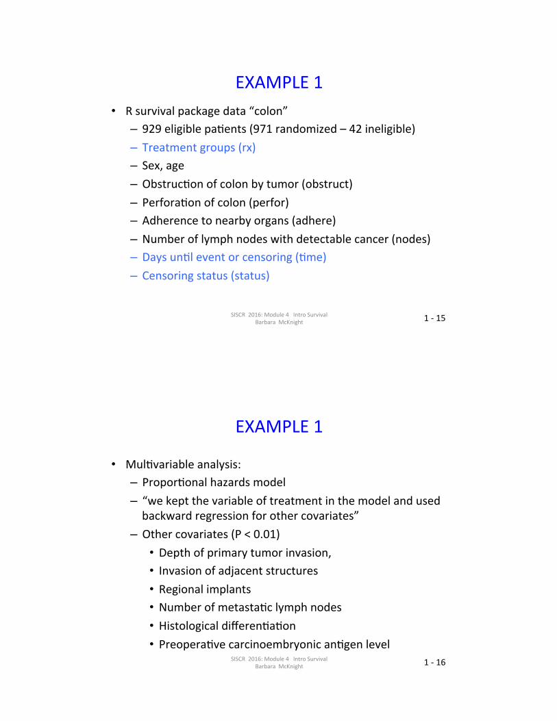
EXAMPLE1• Rsurvivalpackagedata“colon”
– 929eligiblepa>ents(971randomized–42ineligible)– Treatmentgroups(rx)– Sex,age– Obstruc>onofcolonbytumor(obstruct)– Perfora>onofcolon(perfor)– Adherencetonearbyorgans(adhere)– Numberoflymphnodeswithdetectablecancer(nodes)– Daysun>leventorcensoring(>me)– Censoringstatus(status)
SISCR2016:Module4IntroSurvivalBarbaraMcKnight
1-16
EXAMPLE1
• Mul>variableanalysis:– Propor>onalhazardsmodel– “wekeptthevariableoftreatmentinthemodelandusedbackwardregressionforothercovariates”
– Othercovariates(P<0.01)• Depthofprimarytumorinvasion,• Invasionofadjacentstructures• Regionalimplants• Numberofmetasta>clymphnodes• Histologicaldifferen>a>on• Preopera>vecarcinoembryonican>genlevel
SISCR2016:Module4IntroSurvivalBarbaraMcKnight

1-17
EXAMPLE1
• Mul>variableresults:– “A^eradjustmentforminorimbalancesinprognos>cvariablesamongtreatmentarms,therapywithfluorouracilpluslevamisolewasagainfoundtohaveanadvantageoverobserva>on(40%reduc>oninrecurrencerate;P<0.0001).”
– “Levamisolealonehadnodetectableadvantage(2%reduc>oninrecurrencerate;P=0.86).”
SISCR2016:Module4IntroSurvivalBarbaraMcKnight
1-18
EXAMPLE2–ALZHEIMER’S
• Petersenetal.2005,NEJM• Mildcogni>veimpairment• VitaminEandDonepezilandPlacebo• Timefromrandomiza>ontoADdiagnosis• Lengthoftreatment3years• Doubleblind• Outcome:PossibleorprobableAD
SISCR2016:Module4IntroSurvivalBarbaraMcKnight

1-19
EXAMPLE2–ALZHEIMER’S
• 769enrolled• 212developedpossibleorprobableAD• “Therewerenosignificantdifferences…duringthethree
yearsoftreatment”• VitaminEvsPlacebo
– HazardRa>o1.02(95%CI,0.74,1.41),p-value0.91• DonepezilvsPlacebo
– HazardRa>o0.80(95%CI,0.57,1.13),p-value0.42
SISCR2016:Module4IntroSurvivalBarbaraMcKnight
1-20
EXAMPLE2–ALZHEIMER’S
• Prespecifiedanalyses• At6monthsintervals
– DonepezilvsPlacebosignificantlyreducedlikelihoodofprogressiontoADduringthefirst12months(p-value0.04)
– Findingsupportedbysecondaryoutcomemeasures– Subgroup≥1apolipoproteinEϵ4allelessignificantlyreducedlikelihoodofprogressiontoADover3years
– VitaminEvsPlacebo:nosignificantdifferences– VitaminEvsPlacebo:alsonosignificanceforabovesubgroup
SISCR2016:Module4IntroSurvivalBarbaraMcKnight

1-21
EXAMPLE2–RESULTS
• Overallandat6and12months
SISCR2016:Module4IntroSurvivalBarbaraMcKnight
1-22
EXAMPLE2–RESULTS
• APOEϵ4results
SISCR2016:Module4IntroSurvivalBarbaraMcKnight

1-23
EDITORIAL
• “long-awaitedresults”• DonepezilstandardtherapyforAD• “Implica>ons….Enormous”
– Clear-cutnega>vefindingsforVitaminE– Especiallynoteworthy– Despitedearthofevidenceofitsefficacy
– Findingsfordonepezil“muchlessclear”– “notquiteasdisappoin>ng”
SISCR2016:Module4IntroSurvivalBarbaraMcKnight
1-24
EDITORIALCOMMENTS
• “rateofprogression…somewhatlowerinthetreatmentgroupduringthefirstyearofthestudy”
• “bytwoyears,eventhissmalleffecthadwornoff”• Possibleexplana>on:“Reducedsta>s>calpowerlaterinthe
studyasthenumberofsubjectsatriskdeclinedowingtodeath,withdrawalanddevelopmentofAD
• Secondaryanalysessuggest…benefitsworeoff
SISCR2016:Module4IntroSurvivalBarbaraMcKnight

1-25
EXAMPLE2–RESULTS
• Interes>ngsteps…..
SISCR2016:Module4IntroSurvivalBarbaraMcKnight
1-26
“COUNTER”EXAMPLE
• Resuscita>onOutcomesConsor>um– Out-of-hospitalcardiacarrest– Trauma>cinjury
• Prehospitalinterven>ons• Excep>onfrominformedconsent• 10RegionalCenters
– 7US– 3Canada
SISCR2016:Module4IntroSurvivalBarbaraMcKnight

1-27
“COUNTER”EXAMPLE• Times
– Event(cardiacarrest,trauma>cinjury)– 911call– ArrivalofEMS– Treatmentstart– Poten>aloutcomes
• Returnofspontaneouscircula>on(Cardiacarrest)• EDadmission• Survivaltohospitaldischarge• Neurologicallyintactsurvival• 28-daysurvival• 6-monthneurologicaloutcomes
SISCR2016:Module4IntroSurvivalBarbaraMcKnight
1-28
“COUNTER”EXAMPLE
• Timeofinjury/cardiacarrest(ordinarilyunknown)
• 911call• Cardiacarrest:Manydeathsbeforeadmissiontohospital• Trauma:Manydeathswithinthefirst24–48hours
SISCR2016:Module4IntroSurvivalBarbaraMcKnight

1-29
SURVIVALDATAANDFUNCTION
• Originalapplica>onsinbiometryweretosurvival>mesincancerclinicaltrials
• Manyotherapplica>onsinbiometry:eg.diseaseonsetages• Interestcentersnotonlyonaverageormediansurvival>me
butalsoonprobabilityofsurvivingbeyond2years,5years,10years,etc.
• Bestdescribedwiththeen>resurvivalfunc>onS(t).– ForT=asubject’ssurvival>me,S(t)=P[T>t].– Characterizestheen>redistribu>onofsurvival>mesT.
– Givesusefulinforma>onforeacht.SISCR2016:Module4IntroSurvival
BarbaraMcKnight
1-30
SURVIVALFUNCTION
0 2 4 6 8
0.0
0.2
0.4
0.6
0.8
1.0
Survival Function
t
S(t
) =
Pr[
T >
t]
SISCR2016:Module4IntroSurvivalBarbaraMcKnight
1-31
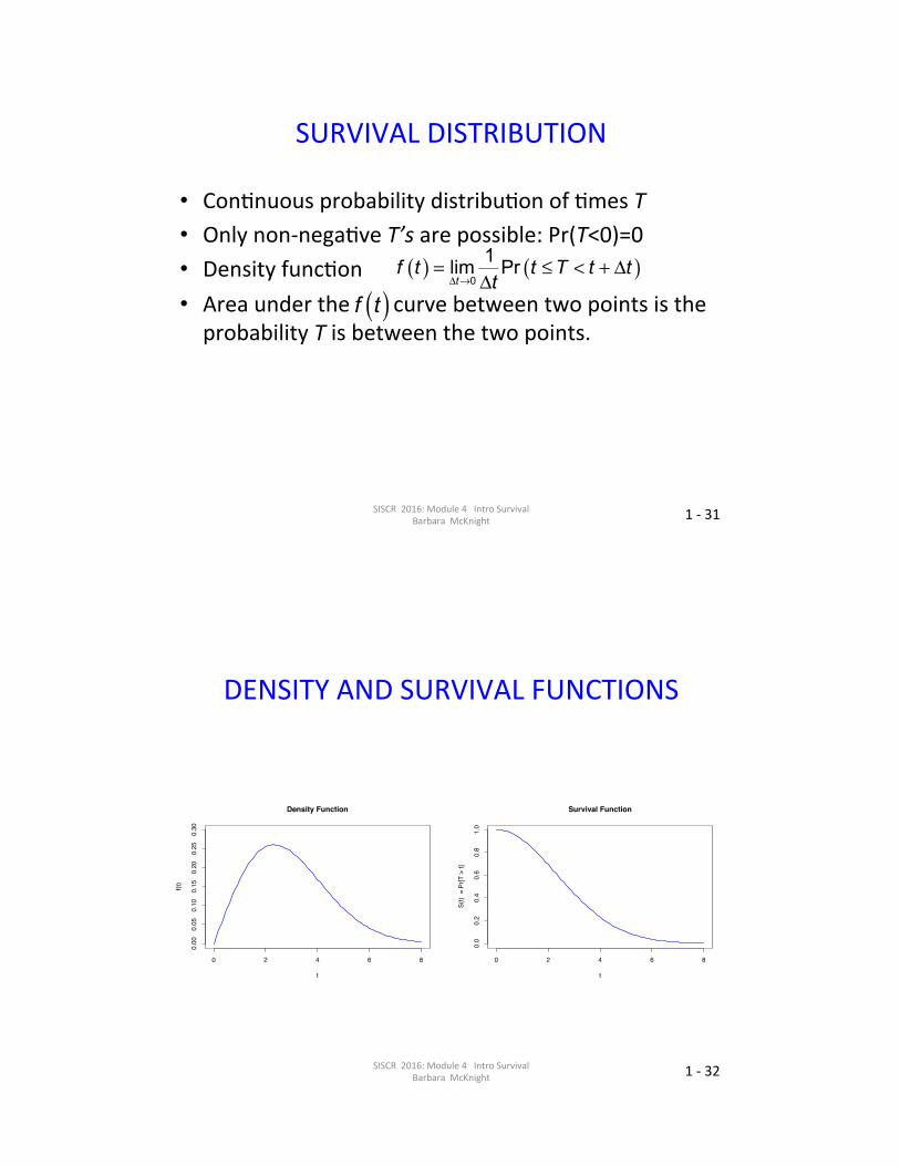
SURVIVALDISTRIBUTION
• Con>nuousprobabilitydistribu>onof>mesT• Onlynon-nega>veT’sarepossible:Pr(T<0)=0• Densityfunc>on• AreaunderthecurvebetweentwopointsistheprobabilityTisbetweenthetwopoints.
( ) ( )Δ →
= ≤ < + ΔΔ01lim Pr
tf t t T t t
t
f t( )
SISCR2016:Module4IntroSurvivalBarbaraMcKnight
1-32
DENSITYANDSURVIVALFUNCTIONS
0 2 4 6 8
0.00
0.05
0.10
0.15
0.20
0.25
0.30
Density Function
t
f(t)
0 2 4 6 8
0.0
0.2
0.4
0.6
0.8
1.0
Survival Function
t
S(t
) =
Pr[
T >
t]
SISCR2016:Module4IntroSurvivalBarbaraMcKnight

1-33
MEDIANSURVIVALTIME
0 2 4 6 8
0.0
0.2
0.4
0.6
0.8
1.0
Median Survival Time
t
S(t
) =
Pr[
T >
t]
median
0.5
SISCR2016:Module4IntroSurvivalBarbaraMcKnight
1-34
MEDIANSURVIVALTIME
0 2 4 6 8
0.00
0.05
0.10
0.15
0.20
0.25
0.30
Density Function
t
f(t)
median
SISCR2016:Module4IntroSurvivalBarbaraMcKnight

1-35
ILLUSTRATIVEDATA
|
|
|
|
|
|
0 2 4 6 8
time
id
|
|
|
|
|
|
65
43
21
D
D
D
D
D
D
id Y1 52 33 6.54 25 46 1
SISCR2016:Module4IntroSurvivalBarbaraMcKnight
1-36
SURVIVALFUNCTIONESTIMATE
• NonparametricEs>mate:reducees>mateby1/nevery>methereisanevent(death):Empiricalsurvivalfunc>ones>mate
0 1 2 3 4 5 6
0.0
0.2
0.4
0.6
0.8
1.0
Survival Function Estimate
t
S(t)
SISCR2016:Module4IntroSurvivalBarbaraMcKnight

1-37
MEDIANESTIMATE
0.0
0.2
0.4
0.6
0.8
1.0
Median Estimate
t
S(t)
1 2 median 4 5 6
SISCR2016:Module4IntroSurvivalBarbaraMcKnight
Byconven>on:medianisearliest>mewheresurvivales>mate≤.5
1-38
OTHERWAYSTODESCRIBEASURVIVALDISTRIBUTION
• Sofarwehavelookedatthedensityfunc>onandsurvivalfunc>onS(t).
• Alsoofinterest:“hazard”func>onλ(t)
• Instantaneousrateatwhichdeathoccursattinthosewhoarealiveatt
• Examples:– Age-specificdeathrate– Age-specificdiseaseincidencerate
SISCR2016:Module4IntroSurvivalBarbaraMcKnight

1-39
HAZARDFUNCTIONFORHUMANS
0 20 40 60 80 100
Human Mortality
age in years
λ(t)
SISCR2016:Module4IntroSurvivalBarbaraMcKnight
1-40
EQUIVALENTCHARACTERIZATIONS
• Anyoneofthedensityfunc>on(f(t)),thesurvivalfunc>on(S(t))orthehazardfunc>on(λ(t))isenoughtodeterminethesurvivaldistribu>on.
• Theyareeachfunc>onsofeachother:
SISCR2016:Module4IntroSurvivalBarbaraMcKnight

1-41
EQUIVALENTCHARACTERIZATIONS
SISCR2016:Module4IntroSurvivalBarbaraMcKnight
0 2 4 6 8
0.0
0.5
1.0
1.5
Hazard Function
t
λ(t)
0 2 4 6 8
0.0
0.4
0.8
Survival Function
t
S(t)
0 2 4 6 8
0.00
0.10
0.20
0.30
Density Function
t
f(t)
1-42
EQUIVALENTCHARACTERIZATIONS
0 2 4 6 8
0.0
0.5
1.0
1.5
Hazard Function
t
λ(t)
0 2 4 6 8
0.0
0.4
0.8
Survival Function
t
S(t)
0 2 4 6 8
0.00
0.10
0.20
0.30
Density Function
t
f(t)
SISCR2016:Module4IntroSurvivalBarbaraMcKnight

1-43SISCR2016:Module4IntroSurvivalBarbaraMcKnight
1-44SISCR2016:Module4IntroSurvivalBarbaraMcKnight

1-45SISCR2016:Module4IntroSurvivalBarbaraMcKnight
1-46SISCR2016:Module4IntroSurvivalBarbaraMcKnight

1-47SISCR2016:Module4IntroSurvivalBarbaraMcKnight
1-48SISCR2016:Module4IntroSurvivalBarbaraMcKnight

1-49SISCR2016:Module4IntroSurvivalBarbaraMcKnight
1-50SISCR2016:Module4IntroSurvivalBarbaraMcKnight
1-51SISCR2016:Module4IntroSurvivalBarbaraMcKnight
1-52SISCR2016:Module4IntroSurvivalBarbaraMcKnight

1-53SISCR2016:Module4IntroSurvivalBarbaraMcKnight
In R
Call up packages we will use (assumes installed)
library(survival)
library(ggplot2)
library(ggfortify)
library(rms)
Get data (in survival package)
data(veteran)

Look at data.
head(veteran)
## trt celltype time status karno diagtime age prior
## 1 1 squamous 72 1 60 7 69 0
## 2 1 squamous 411 1 70 5 64 10
## 3 1 squamous 228 1 60 3 38 0
## 4 1 squamous 126 1 60 9 63 10
## 5 1 squamous 118 1 70 11 65 10
## 6 1 squamous 10 1 20 5 49 0
Survival Curve
Survival time variable, make survival object and get descriptives
Y <- Surv(veteran$time)
Shat <- survfit(Y ~ 1)
Shat
## Call: survfit(formula = Y ~ 1)
##
## n events median 0.95LCL 0.95UCL
## 137 137 80 52 99

Plot Survival Curve
plot(Shat, xlab = "Days", ylab = "Survival Probability")
0 200 400 600 800 1000
0.0
0.2
0.4
0.6
0.8
1.0
Days
Surv
ival P
roba
bilit
y
Plot Survival Curve: Other Options
plot(Shat, conf.int = FALSE, xlab = "Days",
ylab = "Survival Probability")
0 200 400 600 800 1000
0.0
0.2
0.4
0.6
0.8
1.0
Days
Surv
ival P
roba
bilit
y

Using ggplot2 and ggfortify
autoplot(Shat) + labs(x = "Days", y = "Survival Probability")
0%
25%
50%
75%
100%
0 250 500 750 1000Days
Surv
ival P
roba
bilit
y
Adding black and white theme.
autoplot(Shat) + theme_bw() + labs(x = "Days", y = "Survival Probability")
0%
25%
50%
75%
100%
0 250 500 750 1000Days
Surv
ival P
roba
bilit
y

Using rms
Shat2 <- npsurv(Y ~ 1)
survplot(Shat2, xlab = "Days")
Days
0 100 200 300 400 500 600 700 800 900
Surv
ival P
roba
bilit
y
0.0
0.2
0.4
0.6
0.8
1.0
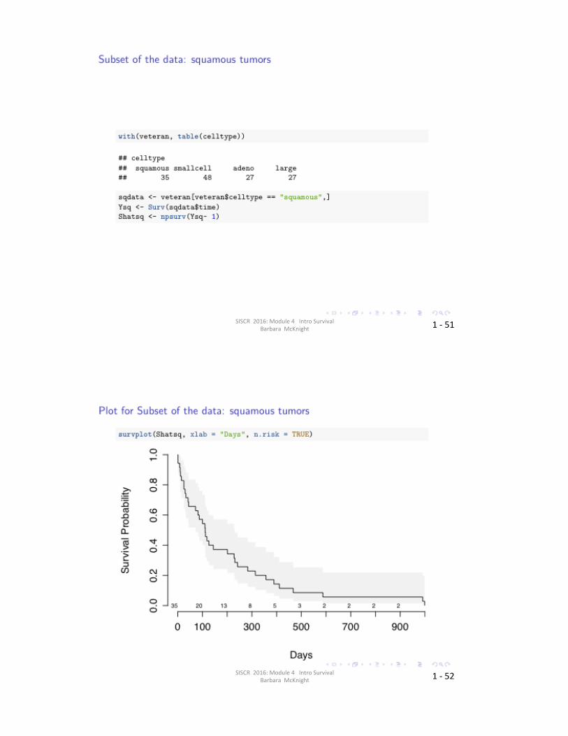
Subset of the data: squamous tumors
with(veteran, table(celltype))
## celltype
## squamous smallcell adeno large
## 35 48 27 27
sqdata <- veteran[veteran$celltype == "squamous",]
Ysq <- Surv(sqdata$time)
Shatsq <- npsurv(Ysq~ 1)
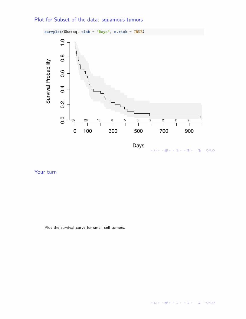
Plot for Subset of the data: squamous tumors
survplot(Shatsq, xlab = "Days", n.risk = TRUE)
Days
0 100 300 500 700 900
Surv
ival P
roba
bilit
y
0.0
0.2
0.4
0.6
0.8
1.0
35 20 13 8 5 3 2 2 2 2
Your turn
Plot the survival curve for small cell tumors.

2-1
Module4:Introduc2ontoSurvivalAnalysisSummerIns2tuteinSta2s2csforClinicalResearch
UniversityofWashingtonJune,2016
BarbaraMcKnight,Ph.D.
ProfessorDepartmentofBiosta2s2csUniversityofWashington
SESSION2:ONE-SAMPLEMETHODS
2-2
OUTLINE
• Session2:– Censoreddata– Risksets– Censoringassump2ons– Kaplan-MeierEs2mator– Medianes2mator– StandarderrorsandCIs
SISCR2016:Module4:IntroSurvivalBarbaraMcKnight

2-3
OUTLINE
• Session2:– Censoreddata– Risksets– Censoringassump2ons– Kaplan-MeierEs2mator– Medianes2mator– StandarderrorsandCIs
SISCR2016:Module4:IntroSurvivalBarbaraMcKnight
2-4
CLINICALTRIAL
SISCR2016:Module4:IntroSurvivalBarbaraMcKnight
|
|
|
|
|
|
0 2 4 6 8
calendar time
id
|
|
|
|
|
|
65
43
21
D
D
L
A
D
D
Start End

2-5
CENSOREDDATA
|
|
|
|
|
|
0 2 4 6 8
survival time
id
65
43
21
D
D
L
A
D
D
SISCR2016:Module4:IntroSurvivalBarbaraMcKnight
2-6
CENSOREDDATA
SISCR2016:Module4:IntroSurvivalBarbaraMcKnight
“Censored”observa2onsgivesomeinforma2onabouttheirsurvival2me.
id Y �1 5 12 3 13 6.5 04 2 05 4 16 1 1|
|
|
|
|
|
0 2 4 6 8
survival time
id
65
43
21
D
D
L
A
D
D

2-7
CENSOREDDATA
SISCR2016:Module4:IntroSurvivalBarbaraMcKnight
“Censored”observa2onsgivesomeinforma2onabouttheirsurvival2me.
id Y �1 5 12 3 13 6.5 04 2 05 4 16 1 1|
|
|
|
|
|
0 2 4 6 8
survival time
id
65
43
21
D
D
L
A
D
D
2-8
ESTIMATION
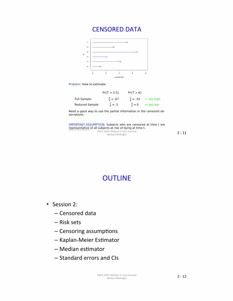
• Canweusethepar2alinforma2oninthecensoredobserva2ons?
• Twooff-the-top-of-the-headanswers:– Fullsample:Yes.Countthemasobserva2onsthatdidnotexperiencetheeventeverandes2mateS(t)asiftherewerenotcensoredobserva2ons.
– Reducedsample:No.Omitthemfromthesampleandes2mateS(t)fromthereduceddataasiftheywerethefulldata.
SISCR2016:Module4:IntroSurvivalBarbaraMcKnight

2-9
CENSOREDDATA
|
|
|
|
|
|
0 2 4 6 8
survival time
id
65
43
21
D
D
L
A
D
D
Problem: How to estimate:
Pr[T > 3.5] Pr[T > 6]
Full Sample: 46 = .67 2
6 = .33
Reduced Sample: 24 = .5 0
4 = 0
SISCR2016:Module4:IntroSurvivalBarbaraMcKnight
2-10
CENSOREDDATA
Based on the data and estimates on the previous page,
Q: Are the Full Sample estimates biased? Why or why not?
A:
Q: Are the Reduced Sample estimates biased? Why or why not?
A:
SISCR2016:Module4:IntroSurvivalBarbaraMcKnight
2-11
CENSOREDDATA
|
|
|
|
|
|
0 2 4 6 8
survival time
id
65
43
21
D
D
L
A
D
D
SISCR2016:Module4:IntroSurvivalBarbaraMcKnight
2-12
OUTLINE
• Session2:– Censoreddata– Risksets– Censoringassump2ons– Kaplan-MeierEs2mator– Medianes2mator– StandarderrorsandCIs
SISCR2016:Module4:IntroSurvivalBarbaraMcKnight

2-13
RISKSETS
|
|
|
|
|
|
0 2 4 6 8
survival time
id
6
5
4
3
2
1
D
D
L
A
D
D
R1 R2 R3 R4
SISCR2016:Module4:IntroSurvivalBarbaraMcKnight
2-14
RISKSETS
|
|
|
|
|
|
0 2 4 6 8
survival time
id
6
5
4
3
2
1
D
D
L
A
D
D
R1{1,2,3,4,5,6}
R2{1,2,3,5}
R3{1,3,5}
R4{1,3}
SISCR2016:Module4:IntroSurvivalBarbaraMcKnight

2-15
CENSOREDDATAASSUMPTION
• Importantassump2on:subjectswhoarecensoredat2metareatthesameriskofdyingattasthoseatriskbutnotcensoredat2met.– Whenwouldyouexpectthistobetrue(orfalse)forsubjectslosttofollow-up?
– Whenwouldyouexpectthistobetrue(orfalse)s2llaliveatthe2meoftheanalysis?
SISCR2016:Module4:IntroSurvivalBarbaraMcKnight
2-16
CENSOREDDATAASSUMPTION
• Importantassump2on:subjectswhoarecensoredat2metareatthesameriskofdyingattasthoseatriskbutnotcensoredat2met.
• Thismeanstherisksetat2metisanunbiasedsampleofthepopula2ons2llaliveat2met.
• Canuseinforma2onfromtheunbiasedrisksetstoes2mateS(t)usingthemethodofKaplanandMeier(Product-LimitEs2mator).
SISCR2016:Module4:IntroSurvivalBarbaraMcKnight

2-17
OUTLINE
• Session2:– Censoreddata– Risksets– Censoringassump2ons– Kaplan-MeierEs2mator– Medianes2mator– StandarderrorsandCIs
SISCR2016:Module4:IntroSurvivalBarbaraMcKnight
2-18
USINGRISKSETSINFOTOESTIMATES(t)
• Repeatedlyusethefactthatfort2>t1,
Pr[T>t2]=Pr[T>t2andT>t1]=Pr[T>t2|T>t1]Pr[T>t1]• Anobserva2oncensoredbetweent1andt2cancontributeto
thees2ma2onofPr[T>t2]byitsunbiasedcontribu2ontoes2ma2onofPr[T>t1].
0 t2t1
SISCR2016:Module4:IntroSurvivalBarbaraMcKnight

2-19
PRODUCT-LIMIT(KAPLAN-MEIER)ESTIMATE
Notation: Let t(1), t(2) . . . , t(J) be the ordered failure times in thesample in ascending order.
t(1) = smallest Y� for which �� = 1 (t(1) = 1 )
t(2) = 2nd smallest Y� for which �� = 1 (t(2) = 3 )...t(J) = largest Y� for which �� = 1 (t(4) = 5 )
Q: Does J = the number of observed deaths in the sample?
A:
Q:When does J = n?
A: SISCR2016:Module4:IntroSurvivalBarbaraMcKnight
2-20
t(j)
|
|
|
|
|
|
0 2 4 6 8
survival time
id
6
5
4
3
2
1
D
D
L
A
D
D
SISCR2016:Module4:IntroSurvivalBarbaraMcKnight

2-21
MORENOTATION
For each t(j):
D(j) = number that die at time t(j)S(j) = number known to have survived beyond t(j)
(by convention: includes those known to have beencensored at t(j))
N(j) = number "at risk" of being observed to die at time t(j)(ie: number still alive and under observation just before t(j))
S(j) = N(j) �D(j)
SISCR2016:Module4:IntroSurvivalBarbaraMcKnight
2-22
FOREXAMPLEDATA● ●● ●
0 2 4 6 8
time
● ●
t(j) N(j) D(j) S(j) Product-limit (Kaplan-Meier) Estimator:
1 6 1 5
3 4 1 3 S(t) = j:t(j)t(1�D(j)N(j)) = j:t(j)t(
S(j)N(j))
4 3 1 25 2 1 1
for t in S(t)
[0, 1) 1 (empty product)
[1,3 ) 1 ⇥ 56 = .833
[3,4 ) 1 ⇥ 56 ⇥
34 = .625
[4,5 ) 1 ⇥ 56 ⇥
34 ⇥
23 = .417
[5,� ) 1 ⇥ 56 ⇥
34 ⇥
23 ⇥
12 = .208SISCR2016:Module4:IntroSurvival
BarbaraMcKnight

2-23
K-MESTIMATOR
0 1 2 3 4 5 6
0.0
0.2
0.4
0.6
0.8
1.0
Survival Function Estimate
t
S(t)
Note:doesnotdescendtozerohere(sincelastobserva2oniscensored).Q: Sincethees2matejumpsonlyatobserveddeath2mes,howdoes
informa2onfromthecensoredobserva2onscontributetoit?A:
SISCR2016:Module4:IntroSurvivalBarbaraMcKnight
2-24
OUTLINE
• Session2:– Censoreddata– Risksets– Censoringassump2ons– Kaplan-MeierEs2mator– Medianes2mator– StandarderrorsandCIs
SISCR2016:Module4:IntroSurvivalBarbaraMcKnight

2-25
MEDIANSURVIVALCENSOREDDATA
0.0
0.2
0.4
0.6
0.8
1.0
Median Estimate, Censored Data
t
S(t)
1 2 3 median 5 6
SISCR2016:Module4:IntroSurvivalBarbaraMcKnight
2-26
OUTLINE
• Session2:– Censoreddata– Risksets– Censoringassump2ons– Kaplan-MeierEs2mator– Medianes2mator– StandarderrorsandCIs
SISCR2016:Module4:IntroSurvivalBarbaraMcKnight

2-27
KMSTANDARDERRORS
Greenwood’s Formula:
•’V�r(S(t)) = S2(t)P
j:t(j)tD(j)
N(j)S(j)
• se(S(t)) =∆’V�r(S(t))
• Pointwise CI: (S(t)� z �2se(S(t)), S(t) + z �
2se(S(t)))
– Can include values < 0 or > 1.
SISCR2016:Module4:IntroSurvivalBarbaraMcKnight
2-28
LOG–LOGKMSTANDARDERRORS
Use complementary log log transformation to keep CI within (0,1):
•’V�r(log(� log(S(t)))) =P
j:t(j)tD(j)
N(j)S(j)
[log(S(t))]2
• se =∆’V�r(log(� log(S(t))))
• CI for log(� log(S(t))) :(log(� log(S(t)))� z �
2se, log(� log(S(t))) + z �
2se)
• CI for S(t) : ([S(t)]ez�/2se , [S(t)]e
�z�/2se)
– CI remains within (0,1).
SISCR2016:Module4:IntroSurvivalBarbaraMcKnight

2-29
GREENWOOD’SFORMULA
0 1 2 3 4 5 6
0.0
0.2
0.4
0.6
0.8
1.0
Survival Function Estimate
t
S(t)
SISCR2016:Module4:IntroSurvivalBarbaraMcKnight
2-30
COMPLEMENTARYLOG-LOG
0 1 2 3 4 5 6
0.0
0.2
0.4
0.6
0.8
1.0
Survival Function Estimate
t
S(t)
SISCR2016:Module4:IntroSurvivalBarbaraMcKnight

2-31
MEDIANCONFIDENCEINTERVAL
Confidence interval for the median is obtained by inverting the signtest of H0 : median = M (Brookmeyer and Crowley, 1982).
• With complete data T1, T2, . . . , Tn, the sign test ofH0 :median = M is performed by seeing if the observedproportion, P[Y > M] is too big (Binomial Distribution orNormal Approximation).
• With censored data (Y1, �1), (Y2, �2), . . . , (Yn, �n) givingincomplete data about T1, T2, . . . , Tn, we cannot always tellwhether T� > M:
When Y� M, �� = 1 observed death before M we know T� MWhen Y� > M death or censored after M we know T� > MWhen Y� M, �� = 0 censored before M we don’t know if
T� M or T� > M
SISCR2016:Module4:IntroSurvivalBarbaraMcKnight
2-32
MEDIANCONFIDENCEINTERVAL
Solution: Following Efron (self-consistency of KM), we estimatePr[T > M] when Y� M, �� = 0 using S(M)
S(Y�).
• For complete data, we let U� =⇢1 T� > M0 T� M
and our test is based onPn
�=1U�.
• For censored data, we let U� =
8<:
1 Y� > MS(M)S(Y�)
Y� M; �� = 00 Y� M; �� = 1
and our test is based onPn
�=1U�.
SISCR2016:Module4:IntroSurvivalBarbaraMcKnight

2-33
MEDIANCONFIDENCEINTERVAL
• It turns out, this is the same as basing our test ofH0 :median = M on a test of H0 : S(M) = 1
2 .
• So a 95% CI for the median contains all potential M for whichthe test of H0 : S(M) = 1
2 cannot reject at � = .05 (2 sided).
• Since S(M) only changes value at observed event times, thetest need only be checked at M = t(1), t(2), . . . , t(J).
• Originally proposed for Greenwood’s formula CIs for S(M), butany good CIs are OK.
• Implemented in many software packages.
SISCR2016:Module4:IntroSurvivalBarbaraMcKnight
2-34
MEDIANCONFIDENCEINTERVAL
Median Confidence Interval, Censored Data
t
S(t)
1 2 3 median 5 6
00.5
1
| ●
SISCR2016:Module4:IntroSurvivalBarbaraMcKnight

2-35
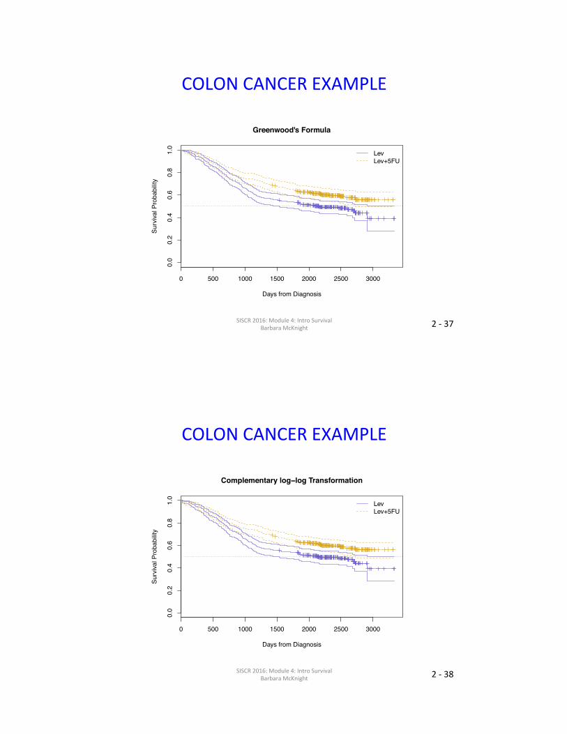
COLONCANCEREXAMPLE
• ClinicaltrialatMayoClinic(Moerteletal.(1990)NEJM)
• StageB2andCcoloncancerpa2ents;adjuvanttherapy
• Threearms– Observa2ononly– Levamisole– 5-FU+Levamisole
• StageCpa2entsonly• Twotreatmentarmsonly
SISCR2016:Module4:IntroSurvivalBarbaraMcKnight
2-36
COLONCANCEREXAMPLE
0 500 1000 1500 2000 2500 3000
0.0
0.2
0.4
0.6
0.8
1.0
Days from Diagnosis
Surv
ival P
roba
bilit
y
LevLev+5FU
SISCR2016:Module4:IntroSurvivalBarbaraMcKnight
2-37
COLONCANCEREXAMPLE
0 500 1000 1500 2000 2500 3000
0.0
0.2
0.4
0.6
0.8
1.0
Days from Diagnosis
Surv
ival P
roba
bilit
yLevLev+5FU
Greenwood's Formula
SISCR2016:Module4:IntroSurvivalBarbaraMcKnight
2-38
COLONCANCEREXAMPLE
0 500 1000 1500 2000 2500 3000
0.0
0.2
0.4
0.6
0.8
1.0
Days from Diagnosis
Surv
ival P
roba
bilit
y
LevLev+5FU
Complementary log−log Transformation
SISCR2016:Module4:IntroSurvivalBarbaraMcKnight

2-39
PRESENTATION
N Events Median(days)
95%CI
LevamisoleOnly
310 161 2152 (1509,∞)
5FU+Levamisole
304 123 -- (2725,∞)
SISCR2016:Module4:IntroSurvivalBarbaraMcKnight
2-40
COLONCANCEREXAMPLE
0 500 1000 1500 2000 2500 3000
0.0
0.2
0.4
0.6
0.8
1.0
Days from Diagnosis
Surv
ival P
roba
bilit
y
LevLev+5FU
Complementary log−log Transformation
SISCR2016:Module4:IntroSurvivalBarbaraMcKnight

2-41
ESTIMATION
• Es2mateS(t)usingKMcurve(nonparametric).– PointwisestandarderrorsandCis– Almostalwayspresented– Notappropriatewhentheeventofinteresthappensonlytosome(moreonthisthistomorrow)
• Median:basedonKMcurve:ouenpresented(tooouen?)
SISCR2016:Module4:IntroSurvivalBarbaraMcKnight
2-42
TOWATCHOUTFOR
• Meansurvival2mehardtoes2matewithoutparametricassump2ons– Censoringmeansincompleteinforma2onaboutlargest2mes
– Meanoverrestricted2meintervalmaybeusefulinsomesevngs(someonthistomorrow)
• Medianes2matemorecomplicatedthanmedianof2mes
• EvenwithCIs,evalua2ngdifferencesbetweencurvesvisuallyissubjec2ve
• Interpreta2onofsurvivalfunc2ones2matesdependsonvalidityofcensoringassump2ons
SISCR2016:Module4:IntroSurvivalBarbaraMcKnight

In R
Load packages.
library(survival)library(rms)
Get data.
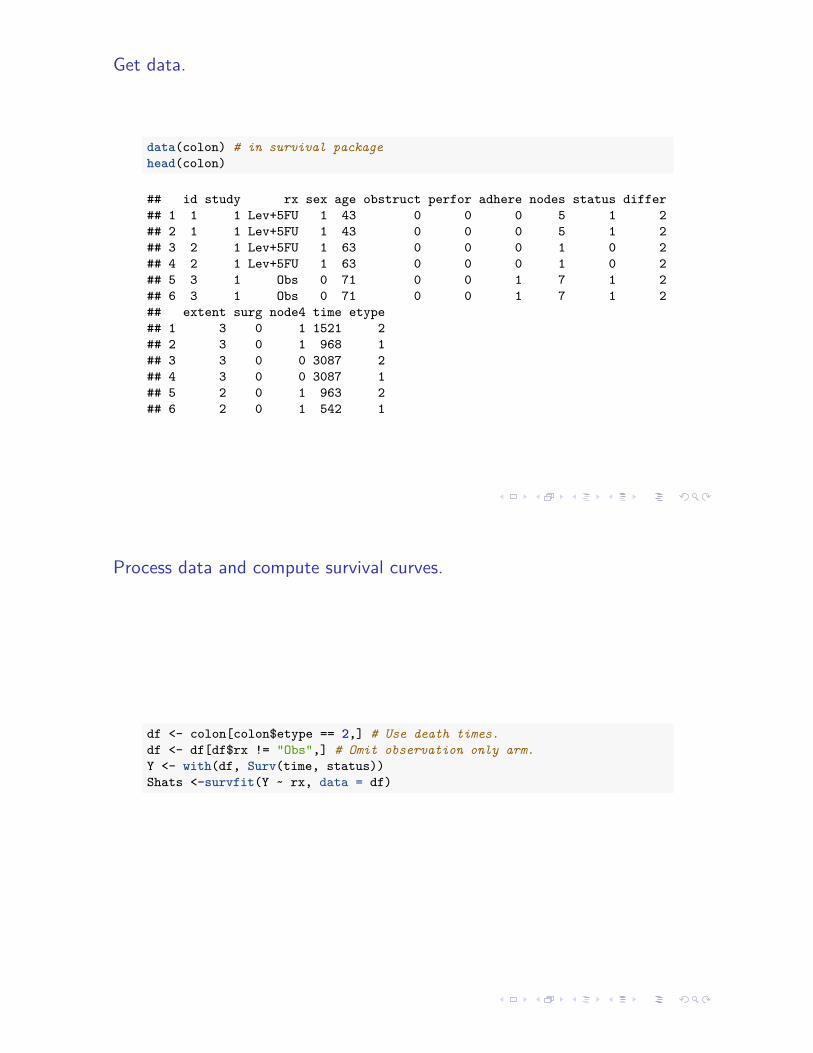
data(colon) # in survival packagehead(colon)
## id study rx sex age obstruct perfor adhere nodes status differ## 1 1 1 Lev+5FU 1 43 0 0 0 5 1 2## 2 1 1 Lev+5FU 1 43 0 0 0 5 1 2## 3 2 1 Lev+5FU 1 63 0 0 0 1 0 2## 4 2 1 Lev+5FU 1 63 0 0 0 1 0 2## 5 3 1 Obs 0 71 0 0 1 7 1 2## 6 3 1 Obs 0 71 0 0 1 7 1 2## extent surg node4 time etype## 1 3 0 1 1521 2## 2 3 0 1 968 1## 3 3 0 0 3087 2## 4 3 0 0 3087 1## 5 2 0 1 963 2## 6 2 0 1 542 1

Process data and compute survival curves.
df <- colon[colon$etype == 2,] # Use death times.df <- df[df$rx != "Obs",] # Omit observation only arm.Y <- with(df, Surv(time, status))Shats <-survfit(Y ~ rx, data = df)
Plot survival curves.
colors <- c("slateblue", "goldenrod")plot(Shats, lty = c(1,2),
col = colors, lwd = 2,xlab = "Days", ylab = "Survival Probability")
legend("bottomleft", lty = c(1,2),col = colors, lwd = 2,legend = c("Lev only", "Lev + 5FU"), bty = "n")

Plot survival curves.
0 500 1000 1500 2000 2500 3000
0.0
0.2
0.4
0.6
0.8
1.0
Days
Surv
ival P
roba
bilit
y
Lev onlyLev + 5FU
With censoring tick marks
plot(Shats, lty = c(1,2),col = colors, lwd = 2,xlab = "Days", ylab = "Probability Survival",mark.time = TRUE)
legend("bottomleft", lty = c(1,2),col = colors, lwd = 2,legend = c("Lev only", "Lev + 5FU"), bty = "n")

With censoring tick marks
0 500 1000 1500 2000 2500 3000
0.0
0.2
0.4
0.6
0.8
1.0
Days
Prob
abilit
y Su
rviva
l
Lev onlyLev + 5FU
With CIs: Greenwood’s formula
ShatsG <- survfit(Y ~ rx, data = df, conf.type = "plain")plot(ShatsG, lty = c(1,2),
col = colors, lwd = 2,xlab = "Days", ylab = "Probability Survival",mark.time = TRUE, conf.int = TRUE)
legend("bottomleft", lty = c(1,2),col = colors, lwd = 2,legend = c("Lev only", "Lev + 5FU"), bty = "n")

With CIs: Greenwood’s formula
0 500 1000 1500 2000 2500 3000
0.0
0.2
0.4
0.6
0.8
1.0
Days
Prob
abilit
y Su
rviva
l
Lev onlyLev + 5FU
With CIs: Complementary log-log formula
ShatsL <-survfit(Y ~ rx, data = df, conf.type = "log-log")plot(ShatsL, lty = c(1,2),
col = colors, lwd = 2,xlab = "Days", ylab = "Probability Survival",mark.time = TRUE, conf.int = TRUE)
legend("bottomleft", lty = c(1,2),col = colors, lwd = 2,legend = c("Lev only", "Lev + 5FU"), bty = "n")
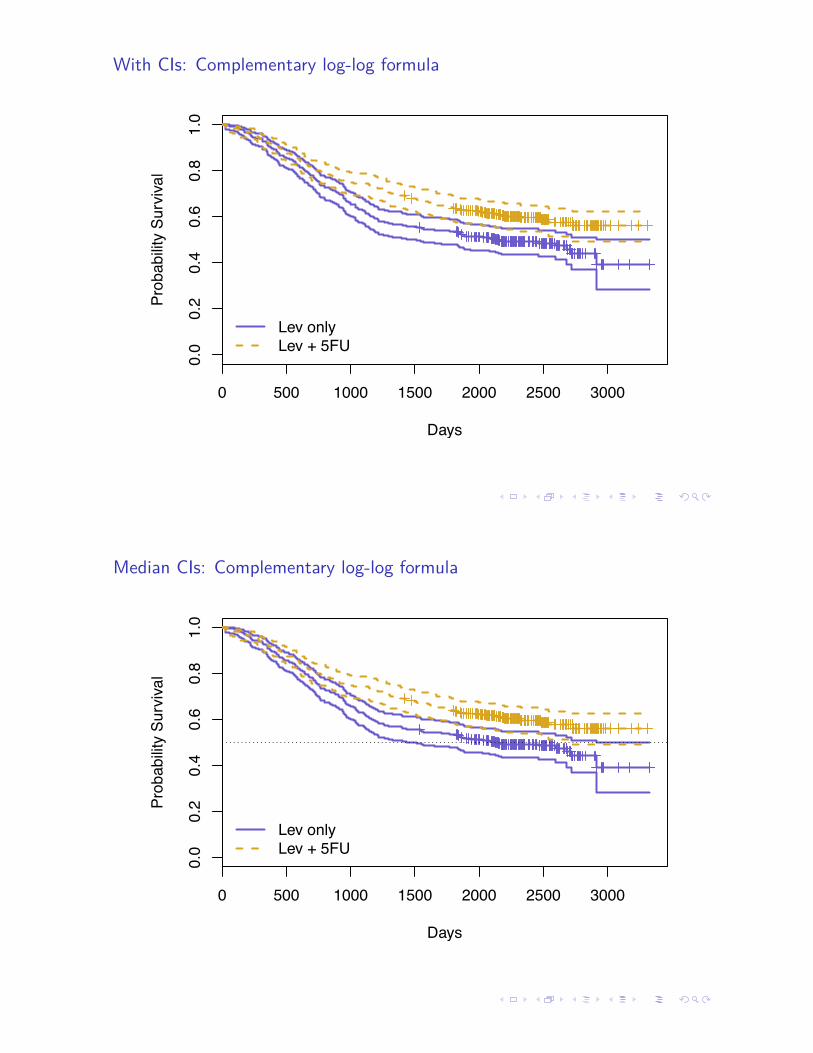
With CIs: Complementary log-log formula
0 500 1000 1500 2000 2500 3000
0.0
0.2
0.4
0.6
0.8
1.0
Days
Prob
abilit
y Su
rviva
l
Lev onlyLev + 5FU
Median CIs: Complementary log-log formula
0 500 1000 1500 2000 2500 3000
0.0
0.2
0.4
0.6
0.8
1.0
Days
Prob
abilit
y Su
rviva
l
Lev onlyLev + 5FU

Median CI summary
ShatsL
## Call: survfit(formula = Y ~ rx, data = df, conf.type = "log-log")#### n events median 0.95LCL 0.95UCL## rx=Lev 310 161 2152 1509 NA## rx=Lev+5FU 304 123 NA 2725 NA
With rms
Shat2 <- npsurv(Y ~ rx, data = df, conf.type = "log-log")survplot(Shat2, xlab = "Days", col = colors)
Days
0 350 700 1400 2100 2800 3500
Surv
ival P
roba
bilit
y
0.0
0.2
0.4
0.6
0.8
1.0
rx=Lev
rx=Lev+5FU

With numbers at risk
survplot(Shat2, xlab = "Days", col = colors, n.risk = TRUE)
Days
0 350 1050 1750 2450 3150
Surv
ival P
roba
bilit
y
0.0
0.2
0.4
0.6
0.8
1.0
310 284 242 198 175 166 135 65 13 3 rx=Lev304 281 245 226 209 195 152 79 26 4 rx=Lev+5FU
rx=Lev
rx=Lev+5FU
With numbers at risk below
par(mar = c(8, 4,4,2) + .1)survplot(Shat2, xlab = "Days", col = colors,
n.risk = TRUE, y.n.risk = -.6)abline(h = .5, lty = 3)

With numbers at risk below
Days
0 350 1050 1750 2450 3150
Surv
ival P
roba
bilit
y
0.0
0.2
0.4
0.6
0.8
1.0
310 284 242 198 175 166 135 65 13 3 rx=Lev304 281 245 226 209 195 152 79 26 4 rx=Lev+5FU
rx=Lev
rx=Lev+5FU
Your turn
1. Using the colon cancer data, plot treatment group survival curves comparingObservation only arm to Levamisole only and Levamisole + 5 FU arms.
2. Compute median survival times and CIs for each group.

3-1
Module4:Introduc2ontoSurvivalAnalysisSummerIns2tuteinSta2s2csforClinicalResearch
UniversityofWashingtonJune,2016
BarbaraMcKnight,Ph.D.
ProfessorDepartmentofBiosta2s2csUniversityofWashington
SESSION3:TWOANDK-SAMPLEMETHODS
3-2
OVERVIEW• Session1
– Introductoryexamples – Thesurvivalfunc2on– SurvivalDistribu2ons– MeanandMediansurvival2me
• Session2 – Censoreddata– Risksets– CensoringAssump2ons– Kaplan-MeierEs2matorandCI– MedianandCI
• Session3 – Two-groupcomparisons:logranktest – Trendandheterogeneitytestsformorethantwogroups
• Session4 – Introduc2ontoCoxregression
SISC2016Module4:IntroSurvivalBarbaraMcKnight

3-3
TESTING
• Groupcomparisons– Twogroups– k-groupheterogeneity– k-grouptrend
• Assume,H0:nodifferencesbetweengroups
SISC 2016 Module 4: Intro Survival Barbara McKnight
3-4
COLONCANCEREXAMPLE
0 500 1000 1500 2000 2500 3000
0.0
0.2
0.4
0.6
0.8
1.0
Days from Diagnosis
Surv
ival P
roba
bilit
y
LevLev+5FU
Complementary log−log Transformation
SISC2016Module4:IntroSurvivalBarbaraMcKnight

3-5
THEP-VALUEQUESTION
• Sta2s2calsignificance?
SISC 2016 Module 4: Intro Survival Barbara McKnight
3-6
COMPARINGSURVIVALDISTRIBUTIONS
• Two-sampledata:comparingS1(t)andS2(t)– (Y1i,δ1i),i=1,…,n1,T�S1(t)– (Y2i,δ2i),i=1,…,n2,T�S2(t)
• CouldlookatS2(t)-S1(t)atasingle2met,butthismightbemisleadingunlessallyoucareaboutissurvivalatthat2me.
SISC2016Module4:IntroSurvivalBarbaraMcKnight

3-7
COMPARISONAT5YEARS
SISC2016Module4:IntroSurvivalBarbaraMcKnight
0.0
0.2
0.4
0.6
0.8
1.0
t
S(t)
5 years
0.0
0.2
0.4
0.6
0.8
1.0
t
S(t)
5 years
3-8
COMPARINGSURVIVALDISTRIBUTIONS
• TherearemanywaystomeasureS2(t)-S1(t),thedistancebetweentwofunc2onsof2me
• Here:focusonmostcommonlyusedtest:thelogranktest,whichcomparesconsistentra2osofhazardfunc2ons
• Module12willconsiderothertests
SISC2016Module4:IntroSurvivalBarbaraMcKnight

3-9
RISKSETS
|
|
|
|
|
|
0 2 4 6 8
survival time
id
6
5
4
3
2
1
D
D
L
A
D
D
R1{1,2,3,4,5,6}
R2{1,2,3,5}
R3{1,3,5}
R4{1,3}
SISC2016Module4:IntroSurvivalBarbaraMcKnight
3-10
LOGRANKTEST
• Thetestisbasedona2x2tableofgroupbycurrentstatusateachobservedfailure2me(ieforeachriskset)
• T(j),j=1,…m,asshownintheTablebelow.
SISC 2016 Module 4: Intro Survival Barbara McKnight
Event/Group 1 2 TotalDie d1(j) d2(j) D(j)
Survive n1(j)-d1(j)=s1(j) n2(j)-d2(j)=s2(j) N(j)-D(j)=S(j)AtRisk n1(j) n2(j) N(j)

3-11
TWO-GROUPCOMPARISONS
• Thecontribu2ontotheteststa2s2cateachevent2meisobtainedbycalcula2ngtheexpectednumberofdeathsinonegroup,assumingthattheriskofdeathatthat2meisthesameineachofthetwogroups.
• Thisyieldstheusual“rowtotal7mescolumntotaldividedbygrandtotal”es2mator.Forexample,forgroup1,theexpectednumberis
• Mostsomwarepackagesbasetheires2matorofthevarianceonthehypergeometricdistribu2on,definedasfollows:
SISC 2016 Module 4: Intro Survival Barbara McKnight
( )( ) ( )
( )= 1
1ˆ j j
jj
n DE
N
V j( ) =n1 j( )n2 j( )D j( ) N j( ) −D j( )( )
N j( )2 N j( ) −1( )
3-12
LOGRANKTWO-GROUPCOMPARISONS
• Eachtestmaybeexpressedintheformofara2oofsumsovertheobservedsurvival2mesasfollows
• Wheretj,j=1,…,J,aretheuniqueorderedevent2mes• Underthenullhypothesisofnodifferenceinsurvivaldistribu2on,thep-
valueforQmaybeobtainedusingthechi-squaredistribu2onwithonedegree-of-freedom,whentheexpectednumberofeventsislarge.
SISC 2016 Module 4: Intro Survival Barbara McKnight
p = Pr χ 21 ≥Q( )
Q =[PJ
j=1(d1(j)�E1(j))]2
V(j)=[PJ
j=1
Ån1(j)n2(j)n1(j)+n2(j)
ãÅd1(j)n1(j)� d2(j)
n2(j)
ã]2
V(j)

3-13
COLONCANCEREXAMPLE
• ComparingLevandLev+5FU:
• Log-ranktest:χ21=8.2,p-value=0.0042
SISC 2016 Module 4: Intro Survival Barbara McKnight
Group N Obs ExpLev 310 161 136.9
Lev+5FU 304 123 147.1Total 614 284 284.0
3-14
LOGRANKTEST
SISC2016Module4:IntroSurvivalBarbaraMcKnight
Othertests(generalizedWilcoxonandothers)cangivemoreweighttoearlyorlatedifferences.
0.0
0.2
0.4
0.6
0.8
1.0
Can Detect This
t
S(t)
0.0
0.2
0.4
0.6
0.8
1.0
But Not This
t
S(t)

3-15
LOGRANKTEST
• Detectsconsistentdifferencesbetweensurvivalcurvesover2me.
• Bestpowerwhen:
– H0:S1(t)=S2(t)foralltvsHA:S1(t)=[S2(t)]c,or
– H0:λ1(t)=λ2(t)foralltvsHA:λ1(t)=cλ2(t)
• Goodpowerwheneversurvivalcurvedifferenceisinconsistentdirec2on
SISC2016Module4:IntroSurvivalBarbaraMcKnight
3-16
STRATIFIEDLOGRANKTEST
• Inalarge-enoughclinicaltrial,confoundingbiasduetoimbalancebetweentreatmentarmsisunlikely.
• However,beterpowercanbeobtainedbyadjus2ngforstronglyprognos2cvariables.
• Onewaytoadjust:stra2fiedlogranktest• CanalsouseCoxregression(Modules8and12)
SISC2016Module4:IntroSurvivalBarbaraMcKnight

3-17
STRATIFIEDLOGRANKTEST
• AssumeRstrata(r=1,…,R)
• Recall(non-stra2fied)log-rankteststa2s2c
• Stra2fiedlog-ranktest
SISC2016Module4:IntroSurvivalBarbaraMcKnight
Q =d1,1 j( ) − E1,1 j( )( )
j1=1
J1
∑ + ...+ d1r j( ) − E1r j( )( ) + ...+ d1R j( ) − E1R j( )( )jR=1
JR
∑jr =1
Jr
∑⎡
⎣⎢
⎤
⎦⎥
2
V1 j( )j1=1
J1
∑ + ...+ Vr j( ) + ...+ VR j( )jR=1
JR
∑jr =1
Jr
∑
Q =[PJ
j=1(d1(j)�E1(j))]2
V(j)
3-18
STRATIFIEDLOG-RANKTEST
• H0: λ1r(t)=λ2r(t)foralltandr=1,…,R• HA:λ1r(t)=cλ2r(t),c≠1,foralltandr=1,…,R
• UnderH0teststa2s2c~χ21whenthenumberofeventsislarge
• The and arebasedsolelyonsubjectsfromtherthstratum
• Willbepowerfulwhendirec2onofgroupdifferenceisconsistentacrossstrataandover2me.
SISC2016Module4:IntroSurvivalBarbaraMcKnight
d1r j( ),E1r j( ) ( )r jV

3-19
EXAMPLE-WHAS
• Example:TheWorcesterHeartAtackStudy(WHAS)• Goal:studyfactorsand2metrends
associatedwithlongtermsurvivalfollowingacutemyocardialinfarc2on(MI)amongresidentsoftheWorcester,MassachusetsStandardMetropolitanSta2s2calArea(SMSA)
• Studybeganin1975• Datacollec2onapproximatelyeveryotheryear• Mostrecentcohort:subjectswhoexperiencedanMIin2001• Themainstudy:over11,000subjects• Here:asmallsamplefromthemainstudywithn=100
SISC2016Module4:IntroSurvivalBarbaraMcKnight
3-20
EXAMPLE-WHAS
• t0: 2meofhospitaladmissionfollowinganacutemyocardialinfarc2on(MI)
• Event:Deathfromanycausefollowinghospitaliza2onforanMI
• Time:Timefromhospitaladmissionto– Death– Endofstudy– Lastcontact
• InterestineffectofgenderadjustedforageSISC2016Module4:IntroSurvival
BarbaraMcKnight

3-21
TESTINGGENDERBYAGEGROUP
survdiff(formula = Yw[age_trend == 46] ~ gender[age_trend == 46], data = whas100)
n=25, 1 observation deleted due to missingness.
N Observed Expected (O-E)^2/E (O-E)^2/Vgender[age_trend == 46]=Male 20 5 6.53 0.357 1.95gender[age_trend == 46]=Female 5 3 1.47 1.584 1.95
Chisq= 1.9 on 1 degrees of freedom, p= 0.163
SISC2016Module4:IntroSurvivalBarbaraMcKnight
3-22
TESTINGGENDERBYAGEGROUP
> survdiff(Yw[age_trend == 65] ~ gender[age_trend == 65], data = whas100)Call:survdiff(formula = Yw[age_trend == 65] ~ gender[age_trend == 65], data = whas100)
n=23, 1 observation deleted due to missingness.
N Observed Expected (O-E)^2/E (O-E)^2/Vgender[age_trend == 65]=Male 17 4 5.6 0.458 2.41gender[age_trend == 65]=Female 6 3 1.4 1.833 2.41
Chisq= 2.4 on 1 degrees of freedom, p= 0.121
SISC2016Module4:IntroSurvivalBarbaraMcKnight

3-23
TESTINGGENDERBYAGEGROUP
> survdiff(Yw[age_trend == 75] ~ gender[age_trend == 75], data = whas100)Call:survdiff(formula = Yw[age_trend == 75] ~ gender[age_trend == 75], data = whas100)
n=22, 1 observation deleted due to missingness.
N Observed Expected (O-E)^2/E (O-E)^2/Vgender[age_trend == 75]=Male 15 10 9.07 0.0947 0.273gender[age_trend == 75]=Female 7 4 4.93 0.1743 0.273
Chisq= 0.3 on 1 degrees of freedom, p= 0.602
SISC2016Module4:IntroSurvivalBarbaraMcKnight
3-24
TESTINGGENDERBYAGEGROUP
> survdiff(Yw[age_trend == 86] ~ gender[age_trend == 86], data = whas100)Call:survdiff(formula = Yw[age_trend == 86] ~ gender[age_trend == 86], data = whas100)
n=30, 1 observation deleted due to missingness.
N Observed Expected (O-E)^2/E (O-E)^2/Vgender[age_trend == 86]=Male 13 9 8.83 0.00318 0.00574gender[age_trend == 86]=Female 17 13 13.17 0.00213 0.00574
Chisq= 0 on 1 degrees of freedom, p= 0.94
SISC2016Module4:IntroSurvivalBarbaraMcKnight

3-25
STRATIFIEDTEST
> survdiff(Yw ~ gender + strata(age_trend), data = whas100)Call:survdiff(formula = Yw ~ gender + strata(age_trend), data = whas100)
n=100, 1 observation deleted due to missingness.
N Observed Expected (O-E)^2/E (O-E)^2/Vgender=Male 65 28 30 0.138 0.402gender=Female 35 23 21 0.197 0.402
Chisq= 0.4 on 1 degrees of freedom, p= 0.526
SISC2016Module4:IntroSurvivalBarbaraMcKnight
3-26
UN-STRATIFIEDTEST
> survdiff(Yw ~ gender, data = whas100)Call:survdiff(formula = Yw ~ gender, data = whas100)
n=100, 1 observation deleted due to missingness.
N Observed Expected (O-E)^2/E (O-E)^2/Vgender=Male 65 28 34.7 1.29 4.06gender=Female 35 23 16.3 2.74 4.06
Chisq= 4.1 on 1 degrees of freedom, p= 0.044
SISC2016Module4:IntroSurvivalBarbaraMcKnight

3-27
WHY?
> with(whas100,table(age_trend, gender)) genderage_trend Male Female 46 20 5 65 17 6 75 15 7 86 13 17
SISC2016Module4:IntroSurvivalBarbaraMcKnight
3-28
WHY?
Age and Gender
Age Group
gend
er
46 65 75 86
Mal
eFe
mal
e
SISC2016Module4:IntroSurvivalBarbaraMcKnight

3-29
HETEROGENEITY
• Whentherearemorethantwogroups,cantestfordifferencesomewherebetweengroups:
• Nullhypothesis:• Alterna2vehypothesis:somewhere
SISC2016Module4:IntroSurvivalBarbaraMcKnight
λ1 t( ) ≡ λ2 t( ) ≡ ...≡ λk t( )≡
3-30
COLONDATA:THREETREATMENTGROUPS
• χ22=11.7(df=onefewerthannumberofgroups)
• P-value:0.003
SISC2016Module4:IntroSurvivalBarbaraMcKnight
ObservedEvents
ExpectedEvents
Obs 161 146.1Lev 123 157.5
Lev+5FU 168 148.4452 452

3-31
TREND
• Whentherearemorethantwo“ordered”groups,itissome2mesofinteresttotestthenullhypothesisofnodifferenceagainsta“trend”alterna2ve
• with<somewhere,or• with>somewhere• Placeboandtwoormoredosesofatherapeu2cagent
• Pre-hypothesized
SISC2016Module4:IntroSurvivalBarbaraMcKnight
λ1 t( ) ≤ λ2 t( ) ≤ ...≤ λk t( ) λ1 t( ) ≥ λ2 t( ) ≥ ...≥ λk t( )
3-32
TREND• Theteststa2s2cfortrenduses“scores”: s1,s2,…,sk
• Nullhypothesis:• Specificalterna2vehypothesis:
• Goodpowerwhenaveragedifferencebetweenobservedandexpectedeventsgrowsordiminisheswithincreasingsi
SISC2016Module4:IntroSurvivalBarbaraMcKnight
λ1 t( ) ≡ λ2 t( ) ≡ ...≡ λk t( )
cs1λ1 t( ) ≡ cs2λ2 t( ) ≡ ...≡ cskλk t( ),c ≠ 1
s ji=1
k
∑ dij −Eij( )j=1
Jk
∑⎛
⎝⎜⎞
⎠⎟
2
′s Vs

3-33
TREND
SISC2016Module4:IntroSurvivalBarbaraMcKnight
Group N Observed Expected
WellDifferen2ated 93 42 47.5
ModeratelyDifferen2ated 663 311 334.9
PoorlyDifferen2ated 150 88 58.6
Tumordifferen2a2onandall-causemortality:
Taronetrendtest:χ12=11.57,P=6.6×10⁻⁴
3-34
SUMMARY
• Canuselogranktesttodetectconsistentdifferences(over2me)inthehazardofdying(theeventoccurring)usingcensoredsurvivaldata– Canstra2fyonprognos2cvariables
• Cantestfordifferencesbetweenmorethantwogroups
• Whenalterna2veisorderedbypriorhypothesis,cantestfortrendratherthanheterogeneity
SISC2016Module4:IntroSurvivalBarbaraMcKnight

3-35
TOWATCHOUTFOR:
• Onlyranksareusedfor“standard”tests• Observa2onswith2me=0• Crossinghazardfunc2ons• P-valuenotvalidifyoudecidebetweentrendandheterogeneitytestamerlookingatthedata– Datatoldyouwhatyourhypothesiswas
SISC2016Module4:IntroSurvivalBarbaraMcKnight
In R
Load packages.
library(survival)library(rms)library(survMisc)library(foreign)

Get data.
data(colon) # in survival packagehead(colon)
## id study rx sex age obstruct perfor adhere nodes status differ## 1 1 1 Lev+5FU 1 43 0 0 0 5 1 2## 2 1 1 Lev+5FU 1 43 0 0 0 5 1 2## 3 2 1 Lev+5FU 1 63 0 0 0 1 0 2## 4 2 1 Lev+5FU 1 63 0 0 0 1 0 2## 5 3 1 Obs 0 71 0 0 1 7 1 2## 6 3 1 Obs 0 71 0 0 1 7 1 2## extent surg node4 time etype## 1 3 0 1 1521 2## 2 3 0 1 968 1## 3 3 0 0 3087 2## 4 3 0 0 3087 1## 5 2 0 1 963 2## 6 2 0 1 542 1
Process data and compute survival curves.
df <- colon[colon$etype == 2,] # Use death times.df <- df[df$rx != "Obs",] # Omit observation only arm.Y <- with(df, Surv(time, status))Shats <-survfit(Y ~ rx, data = df)

Plot survival curves.
colors <- c("slateblue", "goldenrod")plot(Shats, lty = c(1,2),
col = colors, lwd = 2,xlab = "Days", ylab = "Survival Probability")
legend("bottomleft", lty = c(1,2),col = colors, lwd = 2,legend = c("Lev only", "Lev + 5FU"), bty = "n")
Plot survival curves.
0 500 1000 1500 2000 2500 3000
0.0
0.2
0.4
0.6
0.8
1.0
Days
Surv
ival P
roba
bilit
y
Lev onlyLev + 5FU
Logrank test
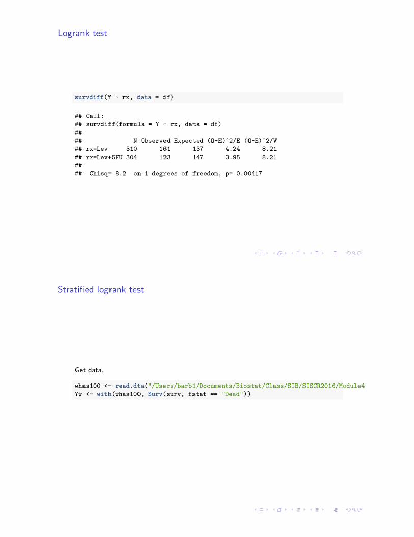
survdiff(Y ~ rx, data = df)
## Call:## survdiff(formula = Y ~ rx, data = df)#### N Observed Expected (O-E)^2/E (O-E)^2/V## rx=Lev 310 161 137 4.24 8.21## rx=Lev+5FU 304 123 147 3.95 8.21#### Chisq= 8.2 on 1 degrees of freedom, p= 0.00417
Stratified logrank test
Get data.
whas100 <- read.dta("/Users/barb1/Documents/Biostat/Class/SIB/SISCR2016/Module4-Intro/whas100.dta")Yw <- with(whas100, Surv(surv, fstat == "Dead"))

Stratum-specific test
survdiff(Yw[age_trend == 46] ~ gender[age_trend == 46], data = whas100)
## Call:## survdiff(formula = Yw[age_trend == 46] ~ gender[age_trend ==## 46], data = whas100)#### n=25, 1 observation deleted due to missingness.#### N Observed Expected (O-E)^2/E (O-E)^2/V## gender[age_trend == 46]=Male 20 5 6.53 0.357 1.95## gender[age_trend == 46]=Female 5 3 1.47 1.584 1.95#### Chisq= 1.9 on 1 degrees of freedom, p= 0.163
Stratum-specific test
survdiff(Yw[age_trend == 65] ~ gender[age_trend == 65], data = whas100)
## Call:## survdiff(formula = Yw[age_trend == 65] ~ gender[age_trend ==## 65], data = whas100)#### n=23, 1 observation deleted due to missingness.#### N Observed Expected (O-E)^2/E (O-E)^2/V## gender[age_trend == 65]=Male 17 4 5.6 0.458 2.41## gender[age_trend == 65]=Female 6 3 1.4 1.833 2.41#### Chisq= 2.4 on 1 degrees of freedom, p= 0.121

Stratum-specific test
survdiff(Yw[age_trend == 75] ~ gender[age_trend == 75], data = whas100)
## Call:## survdiff(formula = Yw[age_trend == 75] ~ gender[age_trend ==## 75], data = whas100)#### n=22, 1 observation deleted due to missingness.#### N Observed Expected (O-E)^2/E (O-E)^2/V## gender[age_trend == 75]=Male 15 10 9.07 0.0947 0.273## gender[age_trend == 75]=Female 7 4 4.93 0.1743 0.273#### Chisq= 0.3 on 1 degrees of freedom, p= 0.602
Stratum-specific test
survdiff(Yw[age_trend == 86] ~ gender[age_trend == 86], data = whas100)
## Call:## survdiff(formula = Yw[age_trend == 86] ~ gender[age_trend ==## 86], data = whas100)#### n=30, 1 observation deleted due to missingness.#### N Observed Expected (O-E)^2/E (O-E)^2/V## gender[age_trend == 86]=Male 13 9 8.83 0.00318 0.00574## gender[age_trend == 86]=Female 17 13 13.17 0.00213 0.00574#### Chisq= 0 on 1 degrees of freedom, p= 0.94

Stratified logrank test
survdiff(Yw ~ gender + strata(age_trend), data = whas100)
## Call:## survdiff(formula = Yw ~ gender + strata(age_trend), data = whas100)#### n=100, 1 observation deleted due to missingness.#### N Observed Expected (O-E)^2/E (O-E)^2/V## gender=Male 65 28 30 0.138 0.402## gender=Female 35 23 21 0.197 0.402#### Chisq= 0.4 on 1 degrees of freedom, p= 0.526
Un-stratified logrank test
survdiff(Yw ~ gender, data = whas100)
## Call:## survdiff(formula = Yw ~ gender, data = whas100)#### n=100, 1 observation deleted due to missingness.#### N Observed Expected (O-E)^2/E (O-E)^2/V## gender=Male 65 28 34.7 1.29 4.06## gender=Female 35 23 16.3 2.74 4.06#### Chisq= 4.1 on 1 degrees of freedom, p= 0.044

Why?
with(whas100,table(age_trend, gender))
## gender## age_trend Male Female## 46 20 5## 65 17 6## 75 15 7## 86 13 17
Why?
mosaicplot(age_trend ~ gender, data = whas100, dir = "v",col = c("slateblue", "goldenrod"), main = "Age and Gender",xlab = "Age Group")
Age and Gender
Age Group
gend
er
46 65 75 86
Mal
eFe
mal
e

Three group test data
df2 <- colon[colon$etype == 2,] # Use death times.Y2 <- with(df2, Surv(time, status))Shats3 <-survfit(Y2 ~ rx, data = df2, conf.type = "log-log")
Three group test
survdiff(Y2 ~ rx, data = df2)
## Call:## survdiff(formula = Y2 ~ rx, data = df2)#### N Observed Expected (O-E)^2/E (O-E)^2/V## rx=Obs 315 168 148 2.58 3.85## rx=Lev 310 161 146 1.52 2.25## rx=Lev+5FU 304 123 157 7.55 11.62#### Chisq= 11.7 on 2 degrees of freedom, p= 0.0029

Trend test function (Dan Gillen)
## survtrend() : Function to compute the Tarone trend test formula : Surv()## response and covariate for trend test data : dataset containing response## and predictor print.table : if TRUE, prints observed and expected failures## under H_0 in each groupsurvtrend <- function(formula, data, print.table = TRUE) {
lrfit <- survdiff(formula, data = data)df <- length(lrfit$n) - 1score <- coxph(formula, data = data)$scoreif (print.table) {
oetable <- cbind(lrfit$n, lrfit$obs, lrfit$exp)colnames(oetable) <- c("N", "Observed", "Expected")print(oetable)
}cat("\nLogrank Test : Chi(", df, ") = ", lrfit$chisq, ", p-value = ", 1 -
pchisq(lrfit$chisq, df), sep = "")cat("\nTarone Test Trend : Chi(1) = ", score, ", p-value = ", 1 - pchisq(score,
1), sep = "")}
Trend test
Shats3t <-survfit(Y2 ~ differ, data = df2, conf.type = "log-log")colors <- c("slateblue", "goldenrod", "forestgreen")plot(Shats3t, lty = c(1:3),
col = colors, lwd = 2,xlab = "Days", ylab = "Survival Probability")
legend("bottomleft", lty = c(1:3),col = colors, lwd = 2,legend = c("Well", "Moderately", "Poorly"), bty = "n")

Trend test
0 500 1000 1500 2000 2500 3000
0.0
0.2
0.4
0.6
0.8
1.0
Days
Surv
ival P
roba
bilit
y
WellModeratelyPoorly
Trend test
survtrend(Y2 ~ differ, data = df2)
## N Observed Expected## differ=1 93 42 47.5287## differ=2 663 311 334.9173## differ=3 150 88 58.5540#### Logrank Test : Chi(2) = 17.18909, p-value = 0.0001851124## Tarone Test Trend : Chi(1) = 11.57379, p-value = 0.0006688778

Your turn
Using the colon cancer data in the survival package with overall survival (after loading
survival package type ?colon for documentation):
1. Perform the logrank test of whether the hazard ratio for all-cause mortality
associated with having more than 4 lymph nodes positive for cancer at diagnosis is
one.
2. Perform the logrank test of whether the hazard ratio for all-cause mortality
associated with having more than 4 lymph nodes positive for cancer at diagnosis is
one after stratification adjustment for treatment arm.
3. Perform the logrank test of whether the all-cause-mortality hazard depends on
extent of disease at diagnosis (heterogeneity test).
4. Perform the logrank test of whether the all-cause-mortality hazard is higher or
lower for greater extent of disease at diagnosis (trend test).
Write a “results” sentence or two for each of these analyses.

4-1
Module4:Introduc1ontoSurvivalAnalysisSummerIns1tuteinSta1s1csforClinicalResearch
UniversityofWashingtonJuly,2016
BarbaraMcKnight,Ph.D.
ProfessorDepartmentofBiosta1s1csUniversityofWashington
SESSION4:INTRODUCTIONTOCOXREGRESSION
4-2
OVERVIEW• Session1
– Introductoryexamples – Thesurvivalfunc1on– SurvivalDistribu1ons– MeanandMediansurvival1me
• Session2 – Censoreddata– Risksets– CensoringAssump1ons– Kaplan-MeierEs1matorandCI– MedianandCI
• Session3 – Two-groupcomparisons:logranktest – Trendandheterogeneitytestsformorethantwogroups
• Session4 – Introduc1ontoCoxregression
SISC2016Module4:IntroSurvivalBarbaraMcKnight

4-3
OUTLINE
• Mo1va1on:– Confoundingandstra1fiedrandomiza1ondesigns
• CoxRegressionmodel– Coefficientinterpreta1on– Es1ma1onandtes1ng– Rela1onshipto2-andK-sampletests
• Examplesthroughout
SISCR2016:Module4IntroSurvivalBarbaraMcKnight
4-4
OUTLINE
• Mo#va#on:– Confoundingandstra#fiedrandomiza#ondesigns
• CoxRegressionmodel– Coefficientinterpreta1on– Es1ma1onandtes1ng– Rela1onshipto2-andK-sampletests
• Examplesthroughout
SISCR2016:Module4IntroSurvivalBarbaraMcKnight

4-5
CONFOUNDING
• Observa1onaldata:some1mesobservedassocia1onsbetweenanexplanatoryvariableandoutcomecanbeduetotheirjointassocia1onwithanothervariable.– Agerelatedtobothsexandriskofdeath.– Otherexamples?
SISCR2016:Module4IntroSurvivalBarbaraMcKnight
4-6
PRECISIONINRCTS
• Becauseofrandomiza1on,confounding/imbalanceusuallynotanissueexceptinsmalltrials.
• Asinlinearregression,regressionmodelsforcensoredsurvivaldataallowgroupcomparisonsamongsubjectswithsimilarvaluesofadjustmentor“precision”variables(morelater).
• Fairerandpossiblymorepowerfulcomparisonaslongasadjustmentvariablesarenottheresultoftreatment.
SISCR2016:Module4IntroSurvivalBarbaraMcKnight
4-7
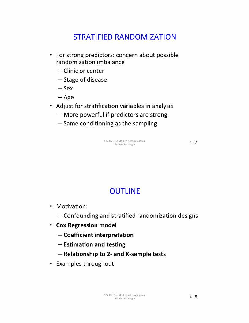
STRATIFIEDRANDOMIZATION
• Forstrongpredictors:concernaboutpossiblerandomiza1onimbalance– Clinicorcenter– Stageofdisease– Sex– Age
• Adjustforstra1fica1onvariablesinanalysis– Morepowerfulifpredictorsarestrong– Samecondi1oningasthesampling
SISCR2016:Module4IntroSurvivalBarbaraMcKnight
4-8
OUTLINE
• Mo1va1on:– Confoundingandstra1fiedrandomiza1ondesigns
• CoxRegressionmodel– Coefficientinterpreta#on– Es#ma#onandtes#ng– Rela#onshipto2-andK-sampletests
• Examplesthroughout
SISCR2016:Module4IntroSurvivalBarbaraMcKnight

4-9
COXREGRESSIONMODEL
SISCR2016:Module4IntroSurvivalBarbaraMcKnight
• Usually written in terms of the hazard function
• As a function of independent variables �1,�2, . . . �k,
�(t) = �0(t)e�1�1+···+�k�k"
relative risk / hazard ratio
log�(t) = log�0(t) + �1�1 + · · · + �k�k"
intercept
4-10
RELATIVERISK/HAZARDRATIO
�(t|�1, . . . ,�k) = �0(t)e�1�1+···+�k�k
�(t|�1,...,�k)�(t|0,...,0) = e�1�1+···+�k�k
SISCR2016:Module4IntroSurvivalBarbaraMcKnight

4-11
REGRESSIONMODELS
LS Linear Regression: Y = �0 + �1�1 + · · · + �k�k + �
Linear: Y ⇠ N(�,�2) � = EY = �0 + �1�1 + · · · + �k�k
Cox: T ⇠ S(t) �(t) = �0(t)e�1�1+···+�k�k
" "Distribution of Dependence of distribution
outcome variable on �1, . . . �k
SISCR2016:Module4IntroSurvivalBarbaraMcKnight
4-12
PROPORTIONALHAZARDSMODEL
SISCR2016:Module4IntroSurvivalBarbaraMcKnight

4-13
EXAMPLE
SISCR2016:Module4IntroSurvivalBarbaraMcKnight
Single binary �:
� =⇢1 Test treatment0 Standard treatment
�(t) = �0(t)e��
Interpretation of e�:
"Relative risk (or hazard ratio) comparing test treatment to stan-dard".
�(t) for � = 1: �0(t)e�·1 = �0(t)e�
�(t) for � = 0: �0(t)e�·0 = �0(t)
ratio: e�(1�0) = e�
4-14
EXAMPLE
SISCR2016:Module4IntroSurvivalBarbaraMcKnight
Proportional Hazards
t
λ(t)
Parallel Log Hazards
t
logλ(t)

4-15
RELATIONSHIPTOSURVIVALFUNCTION
SISCR2016:Module4IntroSurvivalBarbaraMcKnight
4-16
PICTURE
SISCR2016:Module4IntroSurvivalBarbaraMcKnight
t
λ(t)
Hazard Function
t
S(t)
Survival Function

4-17
ESTIMATESANDCONFIDENCEINTERVALS
SISCR2016:Module4IntroSurvivalBarbaraMcKnight
• We estimate � by maximizing the "partial likelihood function"
• Requires iteration on computer
• � is a MPLE (Maximum Partial Likelihood Estimator)
• We do not need to estimate �0(t) to do this
• Most packages will estimate se(�) using the information matrixfrom this PL.
• 95% CI for �: (�� 1.96se(�), �+ 1.96se(�))
• 95% CI for RR = e� : (e��1.96se(�), e�+1.96se(�))
4-18
PARTIALLIKELIHOOD
Data for the �th subject: (t�, ��,�1�, . . .�k�)
For subject with the jth ordered failure time : (t(j),1,�1(j), . . . ,�k(j))
PL(�1, . . . ,�k) =JY
j=1
e�1�1(j)+···+�k�k(j)P
�:t��t(j) e�1�1�+···+�k�k�
• (�1, . . . , �k) are the values of (�1, . . . ,�k) that maximizePL(�1, . . . ,�k). (MPLEs)
• Compares � values for the subject who failed at time t(j) tothose of all subjects at risk at time t(j).
• Does not depend on the values of the t�, only on their order.
• Does not depend on �0(t).
SISCR2016:Module4IntroSurvivalBarbaraMcKnight

4-19
RISKSETPICTURE
SISCR2016:Module4IntroSurvivalBarbaraMcKnight
|
|
|
|
|
|
0 2 4 6 8
survival time
1
1
0
0
0
1
x
D
D
L
A
D
D
1 vs 0.5 0 vs 0.5 1 vs 0.67 1 vs 0.5
Risk Sets and Treatment
4-20
FULLLIKELIHOOD
SISCR2016:Module4IntroSurvivalBarbaraMcKnight
L(�,�0(t)) =Y
Failures
Pr[T = t�]Y
Censorings
Pr[T > t�]
=Y
Failures
�(t�|��)S(t�|��)Y
Censorings
S(t�|��)
=nY
�=1[�(t�|��)]��S(t�|��)
=nY
�=1[�0(t�)e���]��e�
R t�0 �0(s)e��ds

4-21
PARTIALLIKELIHOODLet Ht represent the entire history of failure, censoring and � in thesample before time t.
Then the likelihood can be rewritten as follows:
L(�,�0(t)) =JY
j=1Pr[�th subject fails at t(j)|Ht(j) , some subject fails at t(j)] ·
Pr[Ht(j) , some subject fails at t(j)]
=JY
j=1
�(t(j)|�(j))P�:t��t(j) �(t(j)|��)
·JY
j=1Pr[Ht(j) , some subject fails at t(j)]
=JY
j=1
�0(t(j))e��(j)P�:t��t(j) �0(t(j))e
���·
JY
j=1Pr[Ht(j) , some subject fails at t(j)]
=JY
j=1
e��(j)P
�:t��t(j) e���·
JY
j=1Pr[Ht(j) , some subject fails at t(j)]
= | {z } | {z }Partial Likelihood Depends on �0(·) and �Depends only on �
SISCR2016:Module4IntroSurvivalBarbaraMcKnight
4-22
HYPOTHESISTESTS
SISCR2016:Module4IntroSurvivalBarbaraMcKnight
Three tests of H0 : � = 0 are possible:
1. Wald test: �se(�)
2. (Partial) Likelihood ratio test
3. Score test: (⇡ logrank test)
Likelihood ratio test is best, but requiresfitting full (� = �) and reduced (� = 0) models.
4-23
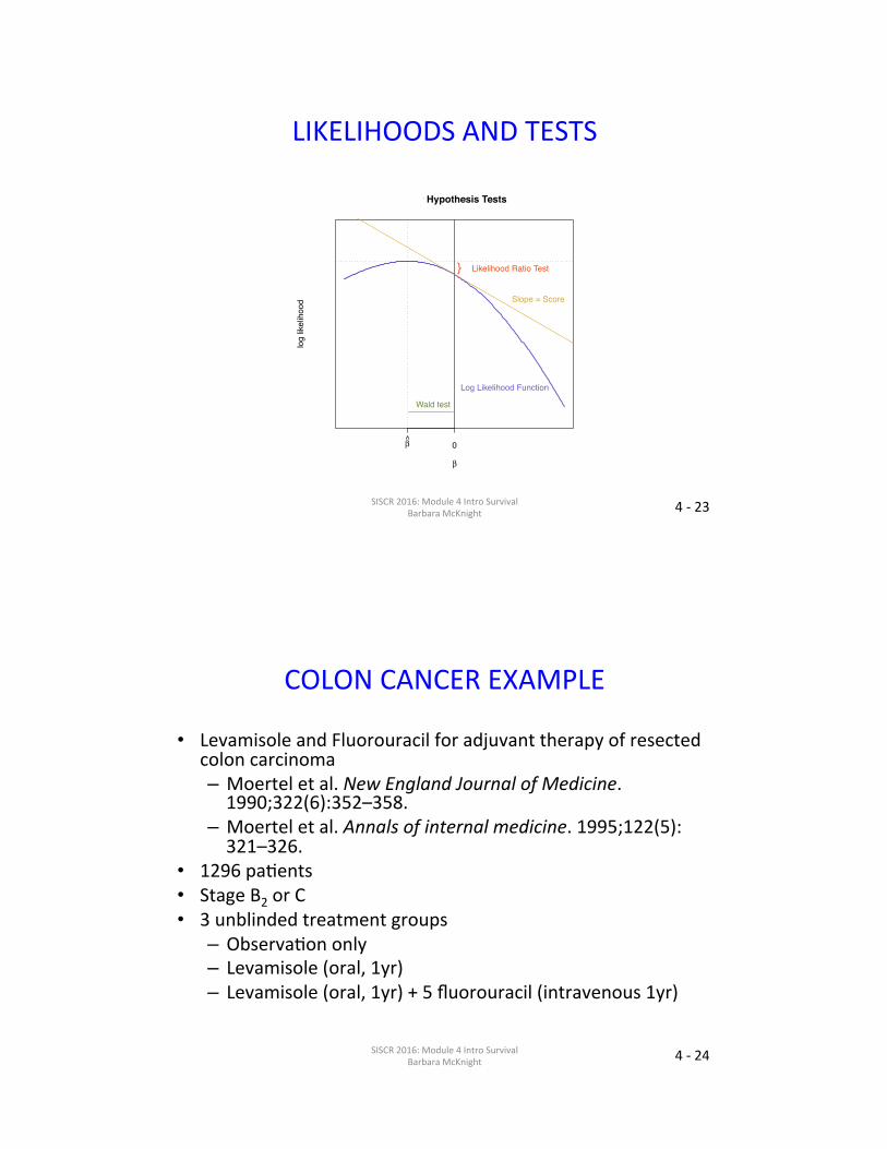
LIKELIHOODSANDTESTS
Four Hypothesis Tests
β
log
likel
ihoo
d
β 0
} Likelihood Ratio Test
Slope = Score
Wald test
Log Likelihood Function
SISCR2016:Module4IntroSurvivalBarbaraMcKnight
4-24
COLONCANCEREXAMPLE
• LevamisoleandFluorouracilforadjuvanttherapyofresectedcoloncarcinoma– Moerteletal.NewEnglandJournalofMedicine.1990;322(6):352–358.
– Moerteletal.Annalsofinternalmedicine.1995;122(5):321–326.
• 1296pa1ents• StageB2orC• 3unblindedtreatmentgroups
– Observa1ononly– Levamisole(oral,1yr)– Levamisole(oral,1yr)+5fluorouracil(intravenous1yr)
SISCR2016:Module4IntroSurvivalBarbaraMcKnight

4-25
COLONCANCEREXAMPLE
• ClinicaltrialatMayoClinic• StageB2andCcoloncancerpa1ents;adjuvanttherapy
• Threearms– Observa1ononly– Levamisole– 5-FU+LevamisoleatMayoClinic
• StageCpa1entsonly• Twotreatmentarmsonly
SISCR2016:Module4IntroSurvivalBarbaraMcKnight
4-26
COLONCANCEREXAMPLE
SISCR2016:Module4IntroSurvivalBarbaraMcKnight
0 500 1000 1500 2000 2500 3000
0.0
0.2
0.4
0.6
0.8
1.0
Days from Diagnosis
Surv
ival P
roba
bilit
y
LevLev+5FU
Complementary log−log Transformation

4-27
COLONCANCEREXAMPLE
Variable
n
Deaths
Hazardra#o
CI
P-value
LevamisoleOnly 310 161 1.0(reference) -- --
Levamisole+5FU 304 123 0.71 (0.56,0.90) .004
SISCR2016:Module4IntroSurvivalBarbaraMcKnight
Q:Whichgrouphasbepersurvival?A:
4-28
TESTCOMPARISON
Test Sta#s#c P-value
Wald’s 8.13 .004
Score 8.21 .004
LikelihoodRa1o 8.21 .004
SISCR2016:Module4IntroSurvivalBarbaraMcKnight
Two-sidedtests

4-29
ANOTHEREXAMPLE
SISCR2016:Module4IntroSurvivalBarbaraMcKnight
Three groups: use indicators for two
�1 =⇢1 Levamisole Only0 otherwise �2 =
⇢1 Levamisole + 5FU0 otherwise
Model: �(t) = �0(t)e�1�1+�2�2
RRs: Levamisole Only vs. Observation e�1Levamisole + 5FU vs. Observation e�2Levamisole + 5FU vs. Levamisole Only e�2��1
4-30
HEURISTICHAZARDS
SISCR2016:Module4IntroSurvivalBarbaraMcKnight
t
λ(t)
Proportional Hazards
t
log(λ(t))
Parallel Log Hazards

4-31
COLONCANCERVariable n Deaths HazardRa#o 95%CI P-value
Observa1onOnly 315 168 1.0(reference) -- --
LevamisoleOnly 310 161 0.97 (0.78,1.21) 0.81
Levamisole+5FU 204 123 0.69 (0.55,0.87) 0.002
SISCR2016:Module4IntroSurvivalBarbaraMcKnight
Q:Whichgrouphasbestsurvival?A:
4-32
TESTCOMPARIOSN
Test Sta#s#c P-value
Wald’s 11.56 .003
Score 11.68 .003
LikelihoodRa1o 12.15 .002
SISCR2016:Module4IntroSurvivalBarbaraMcKnight
Samehypothesisas3-groupheterogeneitytest.Scoretestissameinlargesamples.

4-33
COLONCANCERTRIALDATA
SISCR2016:Module4IntroSurvivalBarbaraMcKnight
0 500 1000 1500 2000 2500 3000
0.0
0.2
0.4
0.6
0.8
1.0
Days from Diagnosis
Surv
ival P
roba
bility
ObsLevLev+5FU
Colon Cancer Trial: All Three Groups
4-34
TREND
• When there are several groups, it is sometimes of interest totest whether risk increases from one group to the next:
– Several dose groups– Other ordered variable– Example: tumor differentiation
• For � =
8<:
1 well differentiated2 moderately differentiated3 poorly differentiated
Model: �(t) = �0(t)e��
• Score test is the same as the trend test
• Could use other values for � (actual dose levels)
SISCR2016:Module4IntroSurvivalBarbaraMcKnight
4-35
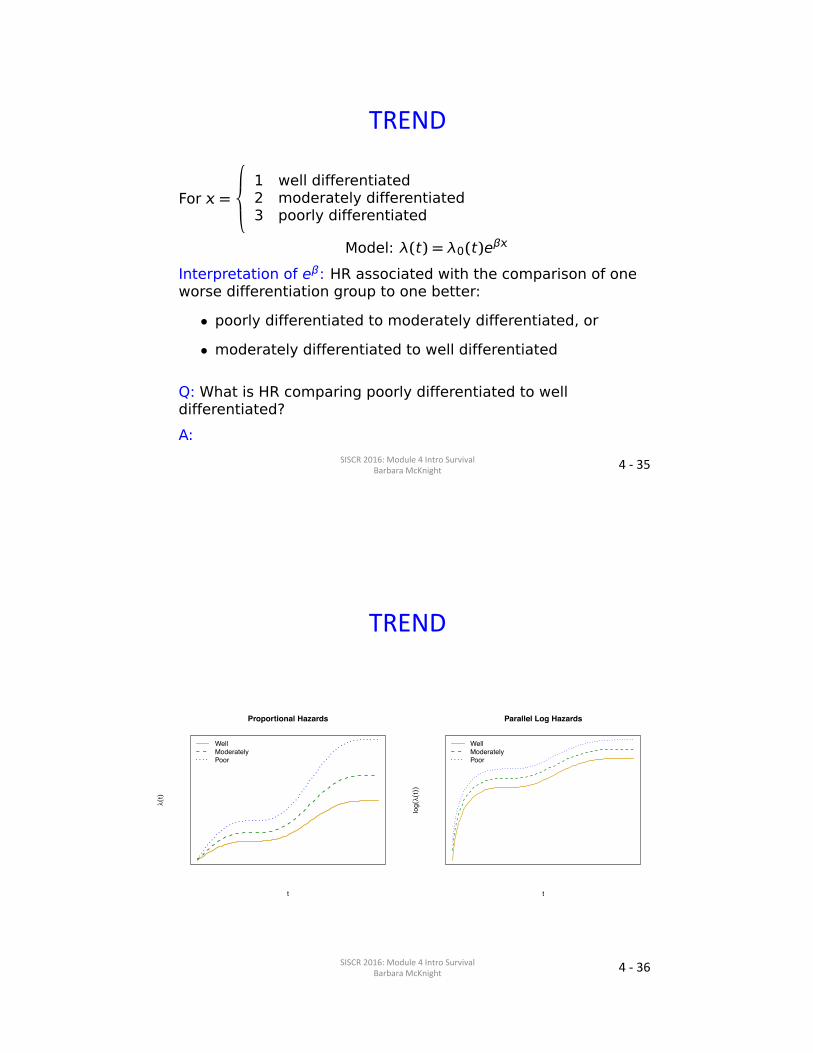
TREND
For � =
8<:
1 well differentiated2 moderately differentiated3 poorly differentiated
Model: �(t) = �0(t)e��
Interpretation of e�: HR associated with the comparison of oneworse differentiation group to one better:
• poorly differentiated to moderately differentiated, or
• moderately differentiated to well differentiated
Q: What is HR comparing poorly differentiated to welldifferentiated?
A:SISCR2016:Module4IntroSurvival
BarbaraMcKnight
4-36
TREND
SISCR2016:Module4IntroSurvivalBarbaraMcKnight
t
λ(t)
WellModeratelyPoor
Proportional Hazards
t
log(λ(t))
WellModeratelyPoor
Parallel Log Hazards

4-37
TRENDWITHDIFFERENTIATION
HazardRa#o
95%CI
Onecategoryworsedifferen1a1on(well,moderately,poor)
1.4 (1.1,1.8)
P=.003(trend)
SISCR2016:Module4IntroSurvivalBarbaraMcKnight
Onepresenta1onbaseden1relyontrend(“groupedlinear”)model:
Ipreferpresen1nghazardra1osandCI’sbasedondummyvariablemodel,andprovidingP-valuefortrend.
4-38
TRENDWITHDIFFERENTIATION
n Deaths HazardRa#o 95%CI
Welldifferen1ated 66 26 1.0(reference) --
Moderatelydifferen1ated
434 196 1.2 (0.80,1.8)
Poorlydifferen1ated
98 54 1.8 (1.2,3.0)
P=.003(trend)
SISCR2016:Module4IntroSurvivalBarbaraMcKnight
Mypreferredpresenta1onbasedondummyvariablemodewithtrendP-value:
Iusuallywouldnotpresentthisforanaprioritrendhypothesis,butforcomparisonhere,theheterogeneityP-value(2df)is0.009.

4-39
TOWATCHOUTFOR:
• CoefficientsinCoxregressionareposi1velyassociatedwithrisk,notsurvival.– Posi1veβmeanslargevaluesofxareassociatedwithshortersurvival.
• Withoutcertaintypesof1me-dependentcovariates,Coxregressiondoesnotdependontheactual1mes,justtheirorder.– Canaddaconstanttoall1mestoremovezeros(somepackagesremoveobserva1onswith1me=0)withoutchanginginference
• ForLRT,nestedmodelsmustbecomparedbasedonsamesubjects.– Ifsomevaluesofvariablesinlargermodelaremissing,thesesubjectsmustberemovedfromfitofsmallermodel.
SISCR2016:Module4IntroSurvivalBarbaraMcKnight
In R
Load packages.
library(survival)library(rms)library(survMisc)library(foreign)
Get data.
data(colon) # in survival packagehead(colon)
## id study rx sex age obstruct perfor adhere nodes status differ## 1 1 1 Lev+5FU 1 43 0 0 0 5 1 2## 2 1 1 Lev+5FU 1 43 0 0 0 5 1 2## 3 2 1 Lev+5FU 1 63 0 0 0 1 0 2## 4 2 1 Lev+5FU 1 63 0 0 0 1 0 2## 5 3 1 Obs 0 71 0 0 1 7 1 2## 6 3 1 Obs 0 71 0 0 1 7 1 2## extent surg node4 time etype## 1 3 0 1 1521 2## 2 3 0 1 968 1## 3 3 0 0 3087 2## 4 3 0 0 3087 1## 5 2 0 1 963 2## 6 2 0 1 542 1
Process data and compute survival curves.
df <- colon[colon$etype == 2,] # Use death times.df <- df[df$rx != "Obs",] # Omit observation only arm.Y <- with(df, Surv(time, status))Shats <-survfit(Y ~ rx, data = df)

Plot survival curves.
0 500 1000 1500 2000 2500 3000
0.0
0.2
0.4
0.6
0.8
1.0
Days
Surv
ival P
roba
bilit
y
Lev onlyLev + 5FU
Fit Cox model
model1 <- coxph(Y ~ rx, data = df)
## Warning in coxph(Y ~ rx, data = df): X matrix deemed to be singular;## variable 2

Results
summary(model1)
## Call:## coxph(formula = Y ~ rx, data = df)#### n= 614, number of events= 284#### coef exp(coef) se(coef) z Pr(>|z|)## rxLev 0.3417 1.4073 0.1199 2.851 0.00436 **## rxLev+5FU NA NA 0.0000 NA NA## ---## Signif. codes: 0 �***� 0.001 �**� 0.01 �*� 0.05 �.� 0.1 � � 1#### exp(coef) exp(-coef) lower .95 upper .95## rxLev 1.407 0.7106 1.113 1.78## rxLev+5FU NA NA NA NA#### Concordance= 0.541 (se = 0.015 )## Rsquare= 0.013 (max possible= 0.996 )## Likelihood ratio test= 8.21 on 1 df, p=0.00416## Wald test = 8.13 on 1 df, p=0.00436## Score (logrank) test = 8.21 on 1 df, p=0.004174
Data with All Three Groups
df2 <- colon[colon$etype == 2,] # Use death times.Y2 <- with(df2, Surv(time, status))

Dummy variable model
model2 <- coxph(Y2 ~ rx, data = df2)
Summary
summary(model2)
## Call:## coxph(formula = Y2 ~ rx, data = df2)#### n= 929, number of events= 452#### coef exp(coef) se(coef) z Pr(>|z|)## rxLev -0.02664 0.97371 0.11030 -0.241 0.80917## rxLev+5FU -0.37171 0.68955 0.11875 -3.130 0.00175 **## ---## Signif. codes: 0 �***� 0.001 �**� 0.01 �*� 0.05 �.� 0.1 � � 1#### exp(coef) exp(-coef) lower .95 upper .95## rxLev 0.9737 1.027 0.7844 1.2087## rxLev+5FU 0.6896 1.450 0.5464 0.8703#### Concordance= 0.536 (se = 0.013 )## Rsquare= 0.013 (max possible= 0.998 )## Likelihood ratio test= 12.15 on 2 df, p=0.002302## Wald test = 11.56 on 2 df, p=0.003092## Score (logrank) test = 11.68 on 2 df, p=0.002906

Trend model
model3 <- coxph(Y2 ~ differ, data = df2)
Summary
summary(model3)
## Call:## coxph(formula = Y2 ~ differ, data = df2)#### n= 906, number of events= 441## (23 observations deleted due to missingness)#### coef exp(coef) se(coef) z Pr(>|z|)## differ 0.32788 1.38803 0.09618 3.409 0.000651 ***## ---## Signif. codes: 0 �***� 0.001 �**� 0.01 �*� 0.05 �.� 0.1 � � 1#### exp(coef) exp(-coef) lower .95 upper .95## differ 1.388 0.7204 1.15 1.676#### Concordance= 0.544 (se = 0.011 )## Rsquare= 0.013 (max possible= 0.998 )## Likelihood ratio test= 11.51 on 1 df, p=0.0006916## Wald test = 11.62 on 1 df, p=0.0006515## Score (logrank) test = 11.57 on 1 df, p=0.0006689
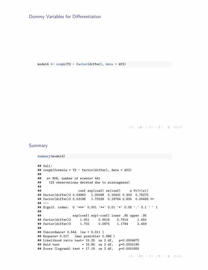
Dummy Variables for Di�erentiation
model4 <- coxph(Y2 ~ factor(differ), data = df2)
Summary
summary(model4)
## Call:## coxph(formula = Y2 ~ factor(differ), data = df2)#### n= 906, number of events= 441## (23 observations deleted due to missingness)#### coef exp(coef) se(coef) z Pr(>|z|)## factor(differ)2 0.04963 1.05088 0.16441 0.302 0.76275## factor(differ)3 0.53196 1.70226 0.18764 2.835 0.00458 **## ---## Signif. codes: 0 �***� 0.001 �**� 0.01 �*� 0.05 �.� 0.1 � � 1#### exp(coef) exp(-coef) lower .95 upper .95## factor(differ)2 1.051 0.9516 0.7614 1.450## factor(differ)3 1.702 0.5875 1.1784 2.459#### Concordance= 0.544 (se = 0.011 )## Rsquare= 0.017 (max possible= 0.998 )## Likelihood ratio test= 15.25 on 2 df, p=0.0004872## Wald test = 16.85 on 2 df, p=0.0002195## Score (logrank) test = 17.19 on 2 df, p=0.0001855

Your turn
Using all-cause mortality as the outcome for the colon data in the survival package in R:
1. Fit a Cox model with a binary treatment indicator relating whether more than 4
lymph nodes were positive for disease at diagnosis is related to the hazard of
all-cause mortality.
2. Fit a Cox model with dummy-variable indicators for whether extent of disease at
diagnosis is related to the hazard of all-cause mortality.
3. Fit a Cox model with “grouped-linear” measure for how extent of disease at
diagnosis is related to the hazard of all-cause mortality.
Write a “results” sentence or two for each of these analyses.