Module 3Introduction to GISLecture 9 – Spatial analysis using GIS

GIS workflow

Data acquisition (geospatial data input)

•GPS

•Remote sensing

•Ortophotos

•LiDAR

Attribute Data Management

•Data verification

•Database management

Exploratory Analysis

•Attribute and spatial data queries

•Geovisualization

Data Analysis

•Vector and raster data analysis

•Terrain mapping

•Spatial interpolation

•Network analysis

Geovisualization

(maps)

Chang, 2014, p.8-9

Spatial Analysis Toolbox

Basic toolbox

Spatial analysis (proximity, overlay)

Projection transformation

Attribute data management

Surface creation

Selection

Extraction

Geovisualization

GIS software

Spatial analysis using vector, raster and attribute table

Spatial analysis use the layers (vector or raster) to obtain new outputs and/or the database

Vector analysis – Buffering (proximity analysis), Overlay and Distance Measurement.

Raster analysis – Local operations (including reclassification) and Distance Measurement.

Attribute analysis – Queries (basic – Identify; advanced – Query Builder)

Spatial analysis operations different for vector and raster

Spatial analysis

Vector

Spatial analysis using vector

The vector data model uses points and their (x,y) coordinates to construct spatial features of points, lines and polygons.

Vector data analysis uses the geometric objects of point, line and polygon as inputs.

(Chang, 2014)

Buffering

• Proximity analysis : “what’s near what?”

• Buffering creates buffer zones by measuring straight-line distances from selected features (points, lines or polygons).

• Appropriate and accurate outputs depend on same measurement units

Diagrams from webhelp.esri.com

Buffering

• Buffering output : buffer zone (a new feature) represented as a polygon containing the selected feature

(source: adapted from http://resources.arcgis.com/en/help/main/10.2/index.html#//000800000019000000 )

Buffering applications

Delimitation of protected zones around features

Defining buffer zones along river streams to restrict urban developments

Creating restrictions criteria for the location of an industrial site based on buffers along conservation areas, river streams, residential areas, …

Definition of areas of influence

Generating a buffer zone centred on a school to estimate the number of potential students

Creating an inclusion zone for an industrial site using buffers along main roads, logistics centres, industrial city areas,…

Buffering applications

Delimitation of protected zones around features

GIS spatial analysis using buffer to identify riparian land use

Buffering applications

Definition of areas of influence

GIS spatial analysis using buffer to define a search radius centred in one specific feature

Overlay

• Overlay analysis : “what’s within what?”

• Overlay creates an output by combining geometries and attributes from different layers (either vector or raster).

• Appropriate and accurate outputs depend on same coordinate system

Overlay

Overlay output: combines two different layers to form a new layer (different geometry and attribute table)

Overlay operations

Union

Intersection

Union• preserves all features from the input and overlay layers• the area extent of the output combines the area extents

of both layers• input layers have to be polygons

Intersect• preserves only those features that fall within the area

extent common to both layers• inputs can take any geometry but the overlay layer is a

polygon• the attribute table contains only data from both layers

(source: adapted from http://resources.arcgis.com/en/help/main/10.2/index.html#/Overlay_analysis/018p00000004000000/ )

Overlay operations

Symmetrical difference • preserves features common to either the input layer or

overlay layer but not both• the geometry of the overlay layer as to be the same as

the input

Identity• preserves only features that fall within the area extent of

the input layer• the overlay layer has to be a polygon or the same

geometry as the input

Symmetrical difference

Identity

(source: adapted from http://resources.arcgis.com/en/help/main/10.2/index.html#/Overlay_analysis/018p00000004000000/ )

Overlay applications

Overlaying watershed boundaries (polygon) with a vegetation layer (polygon) to calculate the amount of each vegetation type in each watershed.

Overlay of different layers to find a specific location suitable for a particular use or susceptible to some risk, for example, overlaying layers representing vegetation type, slope, aspect and soil moisture to find areas susceptible to wildfire.

Logging roads (lines) and vegetation types (polygons) overlayed to create a new line feature class

Distance measurement

Measure of the Euclidean distance (i.e., in a straight line) between spatial features in a vector layer

Proximity analysis: “ How close?”, “What is the distance?” “What is the nearest or farthest feature from something?”

Distance from each point in one feature class to the nearest point or line feature in another feature class.

Example: find the closest stream for a set of wildlife observations or the closest bus stops to a set of tourist destinations

http://resources.esri.com/help/9.3/arcgisengine/java/gp_toolref/geoprocessing/proximity_analysis.htm

Distance measurement

Distance from each point in one feature class to all the points within a given search radius in another feature class.

Example: find the distance and direction to all the water wells within a given distance of a test well where you identified a contaminant

http://resources.esri.com/help/9.3/arcgisengine/java/gp_toolref/geoprocessing/proximity_analysis.htm

Spatial analysis

Raster

Spatial analysis using raster

The raster data model uses a regular grid to cover the space and the value in each grid cell to represent the characteristic of a spatial phenomenon at the cell location.

In contrast with vector data analysis, which uses points, lines and polygons, raster data analysis uses cells and rasters .

(Chang, 2014)

Raster analysis tools

Local Neighbourhood Zonal Global

One-to-one cellOutput value depends on the input value at a cell location and the values of the cells in a specified neighbourhood around that location

Output value depends on the value of the cell at the location and the association that location has within a cartographic zone.

Input

Output

Output value function of all the cells combined from the various input raster datasets

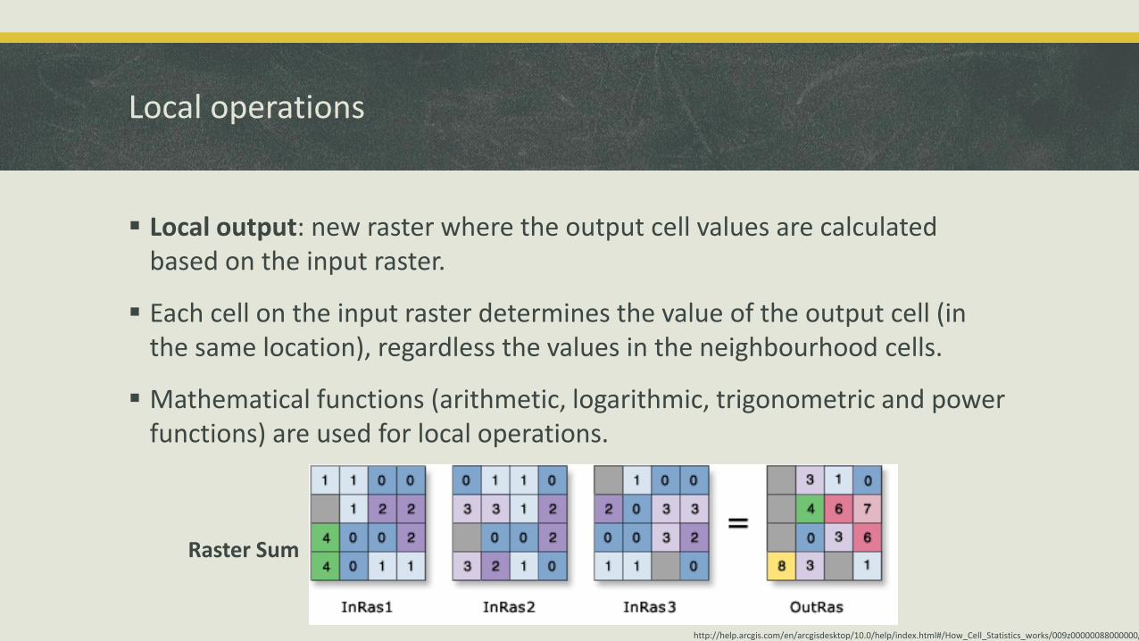
Local operations

Local output: new raster where the output cell values are calculated based on the input raster.

Each cell on the input raster determines the value of the output cell (in the same location), regardless the values in the neighbourhood cells.

Mathematical functions (arithmetic, logarithmic, trigonometric and power functions) are used for local operations.

Raster Sum

http://help.arcgis.com/en/arcgisdesktop/10.0/help/index.html#/How_Cell_Statistics_works/009z00000088000000/

Local operations - Reclassification

Creates a new raster by assigning new cell values based on their interpretation.

Frequently used in GIS projects since it helps simplifying raster data (hence making the results easier to interpret).

It is commonly used to assign different categories in a raster.

Distance measurements

Physical distance (Euclidean distance measured from one cell centre to the other)

Each output cell has the distance to the nearest river feature

Another example: Forest fire model where the distance from a currently burning cell determines next cell burning

Distance measurements

Cost distance (i.e. measuring the cost associated with a physical distance)

Calculates the least accumulative cost distance for each cell to the nearest source over a cost surface.

Measuring cost distance helps to find the least-cost path: the best route for a new road in terms of construction costs; developing a hiking trail system in a national park; finding cost-effective routes between places on delivery routes, national monuments or other destinations

Least-cost path

http://help.arcgis.com/en/arcgisdesktop/10.0/help/index.html#/Understanding_cost_distance_analysis/009z000000z5000000/ and fromhttp://help.arcgis.com/en/arcgisdesktop/10.0/help/index.html#/Creating_the_least_cost_path/009z00000021000000/ )

next weekSCI103 notes:

Go through section 3 - Module 3 in your Learning ModulesThe information presented here is important for Assessment 4a) and Assessment 5.

Start planning Assessment 5 (any questions yet?)