Embed Size (px)
Citation preview

TH
E
U N I V E RS
IT
Y
OF
ED I N B U
RG
H
Modular Bayesian inference
Yufei Cai, Zoubin Ghahramani, Chris Heunen, Ohad Kammar,Sean K. Moss, Klaus Ostermann, Adam Scibior, Sam Staton,
Matthijs Vakar, and Hongseok Yang
Dagstuhl Seminar:Algebraic effects go mainstream
24 April 2018
Cai, Ghahramani, Heunen, Kammar,Moss, Ostermann, Scibior, Staton, Vakar, andYang Modular Bayesian inference

What is statistical probabilistic programming?
Bayesian data modelling
1. Develop a probabilistic (generative) model.
2. Design an inference algorithm for the model.
3. Using the algorithm, fit the model to the data.
Cai, Ghahramani, Heunen, Kammar,Moss, Ostermann, Scibior, Staton, Vakar, andYang Modular Bayesian inference

What is statistical probabilistic programming?
Example
Acidity in soil
pH
distance (km)
Cai, Ghahramani, Heunen, Kammar,Moss, Ostermann, Scibior, Staton, Vakar, andYang Modular Bayesian inference

What is statistical probabilistic programming?
Generative model
s ∼ normal(0, 2)b ∼ normal(0, 6)f(x)= s · x+ byi = normal(f(i), 0.5)
for i = 0 . . . 6
Conditioning
y0 = 0.6, y1 = 0.7, y2 = 1.2, y3 = 3.2, y4 = 6.8, y5 = 8.2, y6 = 8.4
Predict f?
Cai, Ghahramani, Heunen, Kammar,Moss, Ostermann, Scibior, Staton, Vakar, andYang Modular Bayesian inference

What is statistical probabilistic programming?
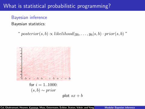
Bayesian inference
Bayesian statistics:
“ posterior(s, b) ∝ likelihood(y0, . . . , y6|s, b) · prior(s, b) ”
“Bayes Law: P (s, b|y0, . . . , y6) =P (y0, . . . , y6|s, b) · P (s, b)
P (y0, . . . , y6)”
for i = 1..1000:(s, b) ∼ prior
(s, b) ∼ posterior
plot sx+ b
Cai, Ghahramani, Heunen, Kammar,Moss, Ostermann, Scibior, Staton, Vakar, andYang Modular Bayesian inference

What is statistical probabilistic programming?
Bayesian inference
Bayesian statistics:
“ posterior(s, b) ∝ likelihood(y0, . . . , y6|s, b) · prior(s, b) ”
posterior(s ≤ s0, b ≤ b0) ∝∫ s0
−∞dse−
s2
2·22∫ b0
−∞dbe−
b2
2·626∏
i=0
e
− (sxi+b−yi)2
2·122
for i = 1..1000:(s, b) ∼ prior
(s, b) ∼ posterior
plot sx+ b
Cai, Ghahramani, Heunen, Kammar,Moss, Ostermann, Scibior, Staton, Vakar, andYang Modular Bayesian inference
What is statistical probabilistic programming?
Bayesian inference
Bayesian statistics:
“ posterior(s, b) ∝ likelihood(y0, . . . , y6|s, b) · prior(s, b) ”
for i = 1..1000:(s, b) ∼ prior
(s, b) ∼ posterior
plot sx+ b
Cai, Ghahramani, Heunen, Kammar,Moss, Ostermann, Scibior, Staton, Vakar, andYang Modular Bayesian inference

What is statistical probabilistic programming?
Bayesian inference
Bayesian statistics:
“ posterior(s, b) ∝ likelihood(y0, . . . , y6|s, b) · prior(s, b) ”
for i = 1..1000:(s, b) ∼ prior (s, b) ∼ posterior
plot sx+ b
Cai, Ghahramani, Heunen, Kammar,Moss, Ostermann, Scibior, Staton, Vakar, andYang Modular Bayesian inference

What is statistical probabilistic programming?
Statistical probabilistic programming
1. Generative models as probabilistic programs simultaneouslymanipulating the:(a) prior; and (b) liklihood(the fundamental concepts in Bayesian statistics)
2. Design an inference algorithm for the model.
3. Using built-in algorithms, approximate the posterior.
Cai, Ghahramani, Heunen, Kammar,Moss, Ostermann, Scibior, Staton, Vakar, andYang Modular Bayesian inference
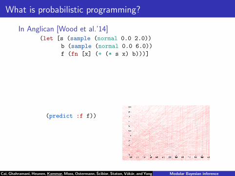
What is probabilistic programming?
In Anglican [Wood et al.’14](let [s (sample (normal 0.0 2.0))
b (sample (normal 0.0 6.0))
f (fn [x] (+ (* s x) b)))]
(predict :f f))
Cai, Ghahramani, Heunen, Kammar,Moss, Ostermann, Scibior, Staton, Vakar, andYang Modular Bayesian inference

What is probabilistic programming?
In Anglican [Wood et al.’14](let [s (sample (normal 0.0 2.0))
b (sample (normal 0.0 6.0))
f (fn [x] (+ (* s x) b)))]
(observe (normal (f 1.0) 0.5) 2.5)
(observe (normal (f 2.0) 0.5) 3.8)
(observe (normal (f 3.0) 0.5) 4.5)
(observe (normal (f 4.0) 0.5) 6.2)
(observe (normal (f 5.0) 0.5) 8.0)
(predict :f f))
Cai, Ghahramani, Heunen, Kammar,Moss, Ostermann, Scibior, Staton, Vakar, andYang Modular Bayesian inference

What is probabilistic programming?
In Anglican [Wood et al.’14](let [sample_linear
(fn [] (let [s (sample (normal 0.0 2.0))
b (sample (normal 0.0 6.0))]
(fn [x] (+ (* s x) b))))
f (sample_linear)]
(observe (normal (f 1.0) 0.5) 2.5)
(observe (normal (f 2.0) 0.5) 3.8)
(observe (normal (f 3.0) 0.5) 4.5)
(observe (normal (f 4.0) 0.5) 6.2)
(observe (normal (f 5.0) 0.5) 8.0)
(predict :f f))
Cai, Ghahramani, Heunen, Kammar,Moss, Ostermann, Scibior, Staton, Vakar, andYang Modular Bayesian inference
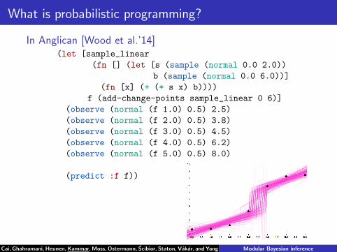
What is probabilistic programming?
In Anglican [Wood et al.’14](let [sample_linear
(fn [] (let [s (sample (normal 0.0 2.0))
b (sample (normal 0.0 6.0))]
(fn [x] (+ (* s x) b))))
f (add-change-points sample_linear 0 6)]
(observe (normal (f 1.0) 0.5) 2.5)
(observe (normal (f 2.0) 0.5) 3.8)
(observe (normal (f 3.0) 0.5) 4.5)
(observe (normal (f 4.0) 0.5) 6.2)
(observe (normal (f 5.0) 0.5) 8.0)
(predict :f f))
Cai, Ghahramani, Heunen, Kammar,Moss, Ostermann, Scibior, Staton, Vakar, andYang Modular Bayesian inference

What is probabilistic programming?
In Anglican [Wood et al.’14](let [sample_linear
(fn [] (let [
b (sample (normal 0.0 6.0))]
(fn [x] b )))
f (add-change-points sample_linear 0 6)]
(observe (normal (f 1.0) 0.5) 2.5)
(observe (normal (f 2.0) 0.5) 3.8)
(observe (normal (f 3.0) 0.5) 4.5)
(observe (normal (f 4.0) 0.5) 6.2)
(observe (normal (f 5.0) 0.5) 8.0)
(predict :f f))
Cai, Ghahramani, Heunen, Kammar,Moss, Ostermann, Scibior, Staton, Vakar, andYang Modular Bayesian inference

What is probabilistic programming?
High-level analogy
graph theorist︷ ︸︸ ︷graph algorithms+
graph savvyhacker︷ ︸︸ ︷
graph library+
user︷ ︸︸ ︷graph manipulating program
inference algorithms︸ ︷︷ ︸statistician
+ inference library︸ ︷︷ ︸statistics savvy
hacker
+ probabilistic program︸ ︷︷ ︸user
Cai, Ghahramani, Heunen, Kammar,Moss, Ostermann, Scibior, Staton, Vakar, andYang Modular Bayesian inference

What is probabilistic programming?
Two effects
▶ Continuous probabilistic choice over the unit intervalI := [0, 1]:
sample : I
▶ Conditioning:
score : R+ → 1 observe(normal(a, b), x) := 1√2πb2
e−(x−a)2
2b2
▶ Monadic semantics: MX is (s-finite) distributions over X:
returnx0 := δx0 ∀a : X → R+.
∫R+
a(x)δx0(dx) = a(x0)
µ >>= f := ν ∀a.∫
a(x)ν(dy) =
∫µ(dx)
∫a(y)f(x)(dy)
sample := UI score r := r · δ⋆Cai, Ghahramani, Heunen, Kammar,Moss, Ostermann, Scibior, Staton, Vakar, andYang Modular Bayesian inference

Why is it hard?
Computing distributions
For t : X we want to:
▶ Plot ⟦t⟧.▶ Sample ⟦t⟧ (e.g., to make prediction)
Challenge 1: Integrals are hard to compute!
This talk: approximate using probabilistic simulation (Monte Carlomethods)Complementary: use symbolic solvers (Maple, MatLab) as inHakaru [Narayanan, Carette, Romano, Shan, and Zinkov, 2016]
Challenge 2
Given a fair coin (12δ1 +12δ0), how do we sample from a biased
coin (pδ1 + (1− p)δ0)?Generalise:Given a prior distribution prior ⟦t⟧, how do we sample from ⟦t⟧?
Cai, Ghahramani, Heunen, Kammar,Moss, Ostermann, Scibior, Staton, Vakar, andYang Modular Bayesian inference
What is inference?
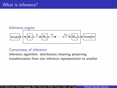
Inference engine
Model SamplerIR1 IR2 IRn· · ·t1 t2 tn−1
Correctness of inferenceInference algorithm: distribution/meaning preservingtransformation from one inference representation to another
Cai, Ghahramani, Heunen, Kammar,Moss, Ostermann, Scibior, Staton, Vakar, andYang Modular Bayesian inference

What is inference?
Challenge 3
▶ Represented data is continuous
▶ Compositional inference representations (IRs)
▶ IRs are higher-order
Traditional measure theory is unsuitable:
Theorem (Aumann’61)
The set Meas(R,R) cannot be made into a measurable space with
eval : Meas(R,R)× R → R
measurable.
Cai, Ghahramani, Heunen, Kammar,Moss, Ostermann, Scibior, Staton, Vakar, andYang Modular Bayesian inference

Contribution
Inference engine
Model SamplerIR1 IR2 IRn· · ·t1 t2 tn−1
Correctness of inference
▶ Modular validation of inference algorithms:Sequential Monte Carlo, Trace Markov Chain Monte CarloBy combining:
▶ Synthetic measure theory [Kock’12]: measure theory withoutmeasurable spaces
▶ Quasi-Borel spaces: a convenient category for higher-ordermeasure theory [LICS’17]
Cai, Ghahramani, Heunen, Kammar,Moss, Ostermann, Scibior, Staton, Vakar, andYang Modular Bayesian inference

Representations
Model SamplerIR1 IR2 IRn· · ·t1 t2 tn−1
Program representation
A representation T = (T , returnT , >>=T ,mT ) consists of:
▶ (T , returnT , >>=T ): monadic interface;
▶ mTX : T X → MX: meaning morphism for every space X
and mT preserves returnT and >>=T :
m(returnT x) = returnM x = δx
m(a >>=T f) = (ma) >>=M λx. m(f x) =
�m(f x)ma(dx)
Cai, Ghahramani, Heunen, Kammar,Moss, Ostermann, Scibior, Staton, Vakar, andYang Modular Bayesian inference

Representations
Model SamplerIR1 IR2 IRn· · ·t1 t2 tn−1
Example representation: lists
instance Rep (List)wherereturnx = [x]xs >>= f = foldr [ ]
(λ(x, ys).f(x) ++ ys) xs
mList[x1, . . . , xn]=∑n
i=1 δxi
Cai, Ghahramani, Heunen, Kammar,Moss, Ostermann, Scibior, Staton, Vakar, andYang Modular Bayesian inference
Representations
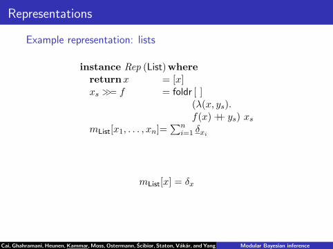
Example representation: lists
instance Rep (List)wherereturnx = [x]xs >>= f = foldr [ ]
(λ(x, ys).f(x) ++ ys) xs
mList[x1, . . . , xn]=∑n
i=1 δxi
mList[x] = δx
Cai, Ghahramani, Heunen, Kammar,Moss, Ostermann, Scibior, Staton, Vakar, andYang Modular Bayesian inference

Representations
Example representation: lists
instance Rep (List)wherereturnx = [x]xs >>= f = foldr [ ]
(λ(x, ys).f(x) ++ ys) xs
mList[x1, . . . , xn]=∑n
i=1 δxi
mList
([x1, . . . , xn] >>=
List f)= m
(f(x1) ++ · · ·++ f(xn)
)=
n∑i=1
mf(xi) =
n∑i=1
�mList ◦f(y)δxi(dy) =
�m ◦f(y)
n∑i=1
δxi(dy)
=
�m ◦f(y)m[x1, . . . , xn](dy) = m[x1, . . . , xn] >>=
M (m ◦f)
Cai, Ghahramani, Heunen, Kammar,Moss, Ostermann, Scibior, Staton, Vakar, andYang Modular Bayesian inference

Representations
Sampling representation
(T , returnT , >>=T ,mT , sampleT )
▶ (T , returnT , >>=T ,mT ): program representation
▶ sampleT : 1 → T Iand mT ◦sampleT = UI
Conditioning representation
(T , returnT , >>=T ,mT , scoreT )
▶ (T , returnT , >>=T ,mT ): program representation
▶ scoreT : [0,∞) → T 1
and mT ◦ scoreT r = r · δ()
Cai, Ghahramani, Heunen, Kammar,Moss, Ostermann, Scibior, Staton, Vakar, andYang Modular Bayesian inference

Representations
Example: free sampler
Samα B {Returnα∣∣ Sample (I → Samα)}:
instance Sampling Rep (Sam)wherereturnx = Returnxa >>= f = match awith {
Returnx→f(x)Sample k→Sample (λr. k(r) >>= f)}
sample = Sampleλr. (Return r)ma = match awith {
Returnx→δxSample k→
�Im(k(x))U(dx)}
Cai, Ghahramani, Heunen, Kammar,Moss, Ostermann, Scibior, Staton, Vakar, andYang Modular Bayesian inference

Representations
Inference representation
(T , returnT , >>=T , sampleT scoreT ,mT ): sampling andconditioning
Example: weighted sampler
WSamX := WSamX = Sam([0,∞)×X)
Cai, Ghahramani, Heunen, Kammar,Moss, Ostermann, Scibior, Staton, Vakar, andYang Modular Bayesian inference

Inference transformations
t : T → S
t : T X → S X for every space X such that:
mS ◦ t = mT
A single compositional step in an inference algorithm
Unnaturality
aggrX : List(R+ ∗X) → List(R+ ∗X)aggregating (r, x), (s, x) to (r + s, x)Then aggr : List → List but not natural:
aggr ◦ List! [(12 ,False), (12 ,True)] = aggr [(12 , ()), (
12 , ())]
= [(1, ())] = [(12 , ()), (12 , ())]
= Enum! [(12 ,False), (12 ,True)] = Enum!◦aggr [(12 ,False), (
12 ,True)]
Cai, Ghahramani, Heunen, Kammar,Moss, Ostermann, Scibior, Staton, Vakar, andYang Modular Bayesian inference

MonadBayes: Modular implementation in Haskell
Performance evaluation (1)
0 200 400 600 800 10000.0
0.5
1.0
1.5
2.0
Exec
utio
n tim
e [s
]
MH100
LR
0 200 400 600 800 10000
1
2
3SMC100
0 200 400 600 800 10000.0
2.5
5.0
7.5
10.0
RMSMC10-1
0 200 400 600 800 10000.0
0.5
1.0
1.5
2.0
Exec
utio
n tim
e [s
]
HMM
0 200 400 600 800 10000
1
2
3
0 200 400 600 800 10000.0
2.5
5.0
7.5
10.0
0 500 1000 1500 2000 2500Dataset size
0
1
2
3
4
Exec
utio
n tim
e [s
]
LDA
0 500 1000 1500 2000 2500Dataset size
0
2
4
6
8
10
0 500 1000 1500 2000 2500Dataset size
0
20
40
60
80
OursAnglicanWebPPL
Cai, Ghahramani, Heunen, Kammar,Moss, Ostermann, Scibior, Staton, Vakar, andYang Modular Bayesian inference

MonadBayes: Modular implementation in Haskell
Performance evaluation (2)
200 400 600 800 10000.0
0.5
1.0
1.5
Exec
utio
n tim
e [s
]
MH
LR50
200 400 600 800 10000
1
2
3SMC
20 40 60 80 100
2
4
6
8
RMSMC10
200 400 600 800 10000.0
0.2
0.4
0.6
0.8
Exec
utio
n tim
e [s
]
HMM20
200 400 600 800 10000.00
0.25
0.50
0.75
1.00
1.25
20 40 60 80 100
2
4
6
200 400 600 800 1000Number of steps
0.25
0.50
0.75
1.00
1.25
Exec
utio
n tim
e [s
]
LDA50
200 400 600 800 1000Number of particles
0
1
2
3
4
20 40 60 80 100Number of rejuvenation steps
5
10
15
OursAnglicanWebPPL
Cai, Ghahramani, Heunen, Kammar,Moss, Ostermann, Scibior, Staton, Vakar, andYang Modular Bayesian inference

Contribution
Inference engine
Model SamplerIR1 IR2 IRn· · ·t1 t2 tn−1
Correctness of inference
▶ Modular validation of inference algorithms:Sequential Monte Carlo, Trace Markov Chain Monte CarloBy combining:
▶ Synthetic measure theory [Kock’12]: measure theory withoutmeasurable spaces
▶ Quasi-Borel spaces: a convenient category for higher-ordermeasure theory [LICS’17]
Cai, Ghahramani, Heunen, Kammar,Moss, Ostermann, Scibior, Staton, Vakar, andYang Modular Bayesian inference

Conclusion
Summary
▶ Bayesian inference: (continuous) sampling and conditioning
▶ Inference representation: monadic interface, sampling,conditioning, and meaning
▶ Plenty of opportunities for traditional programming languageexpertise
Further topics
▶ Sequential Monte Carlo (SMC)
▶ Markov Chain Monte Carlo (MCMC) andMetropolis-Hastings-Green Theorem for Qbs
▶ Combining SMC and MCMC into Move-Resample SMC
Cai, Ghahramani, Heunen, Kammar,Moss, Ostermann, Scibior, Staton, Vakar, andYang Modular Bayesian inference