This article was downloaded by: [Simon Fraser University]On: 20 June 2013, At: 02:51Publisher: Taylor & FrancisInforma Ltd Registered in England and Wales Registered Number: 1072954 Registeredoffice: Mortimer House, 37-41 Mortimer Street, London W1T 3JH, UK

Engineering OptimizationPublication details, including instructions for authors andsubscription information:http://www.tandfonline.com/loi/geno20

Modification of DIRECT for high-dimensional design problemsArash Tavassoli a , Kambiz Haji Hajikolaei a , Soheil Sadeqi a , G.Gary Wang a & Erik Kjeang aa School of Mechatronic Systems Engineering, Simon FraserUniversity , Surrey , BC , CanadaPublished online: 19 Jun 2013.

To cite this article: Arash Tavassoli , Kambiz Haji Hajikolaei , Soheil Sadeqi , G. Gary Wang &Erik Kjeang (2013): Modification of DIRECT for high-dimensional design problems, EngineeringOptimization, DOI:10.1080/0305215X.2013.800057

To link to this article: http://dx.doi.org/10.1080/0305215X.2013.800057

PLEASE SCROLL DOWN FOR ARTICLE

Full terms and conditions of use: http://www.tandfonline.com/page/terms-and-conditions

This article may be used for research, teaching, and private study purposes. Anysubstantial or systematic reproduction, redistribution, reselling, loan, sub-licensing,systematic supply, or distribution in any form to anyone is expressly forbidden.

The publisher does not give any warranty express or implied or make any representationthat the contents will be complete or accurate or up to date. The accuracy of anyinstructions, formulae, and drug doses should be independently verified with primarysources. The publisher shall not be liable for any loss, actions, claims, proceedings,demand, or costs or damages whatsoever or howsoever caused arising directly orindirectly in connection with or arising out of the use of this material.

Engineering Optimization, 2013http://dx.doi.org/10.1080/0305215X.2013.800057

Modification of DIRECT for high-dimensional design problems

Arash Tavassoli, Kambiz Haji Hajikolaei, Soheil Sadeqi, G. Gary Wang* and Erik Kjeang

School of Mechatronic Systems Engineering, Simon Fraser University, Surrey, BC, Canada

(Received 23 November 2012; final version received 1 April 2013)

DIviding RECTangles (DIRECT), as a well-known derivative-free global optimization method, has beenfound to be effective and efficient for low-dimensional problems. When facing high-dimensional black-box problems, however, DIRECT’s performance deteriorates. This work proposes a series of modificationsto DIRECT for high-dimensional problems (dimensionality d > 10). The principal idea is to increase theconvergence speed by breaking its single initialization-to-convergence approach into several more intricatesteps. Specifically, starting with the entire feasible area, the search domain will shrink gradually andadaptively to the region enclosing the potential optimum. Several stopping criteria have been introduced toavoid premature convergence.A diversification subroutine has also been developed to prevent the algorithmfrom being trapped in local minima. The proposed approach is benchmarked using nine standard high-dimensional test functions and one black-box engineering problem. All these tests show a significantefficiency improvement over the original DIRECT for high-dimensional design problems.

Keywords: global optimization; DIRECT method; high dimensional problems

1. Introduction

Global optimization (GO) methods can be roughly classified into deterministic and stochasticapproaches. Stochastic methods use random sampling; hence different runs may result in differentoutcomes for an identical problem. Genetic algorithm (GA) (Goldberg 1989), simulated annealing(SA) (Kirkpatrick, Gelatt, and Vecchi 1983) and particle swarm optimization (PSO) (Kennedy andEberhart 1995) are well-known representatives of this class. In contrast, deterministic methodswork based on a predetermined sequence of point sampling, converging to the global optimum;therefore different runs result in the identical answer for the same optimization problem. Branchand bound (Lawler and Wood 1966) and DIviding RECTangles (DIRECT) (Jones, Perttunen, andStuckman 1993; Jones 2001) are examples of this category. This work aims to optimize high-dimensional, expensive and black-box (HEB) functions. In science and engineering, these threefactors make the optimization procedure very challenging. First, high dimensionality makes thesearch space huge and the systematic searching intractable. This results in a difficulty called the‘curse-of-dimensionality’. Secondly, computationally expensive problems are those with time-consuming procedures of function evaluations and usually consist of a simulation as finite elementanalysis (FEA) or computational fluid dynamics (CFD). This factor brings up a limitation in thenumber of function calls for application of optimization in practice. Lastly, black-box functionsare those with no explicit function or formula that makes gradient-based optimization methods

*Corresponding author. Email: gary_wang@sfu.ca

© 2013 Taylor & Francis

Dow

nloa

ded

by [

Sim

on F

rase

r U

nive

rsity

] at

02:

51 2

0 Ju

ne 2

013

2 A. Tavassoli et al.

impossible to use. One possible way of dealing with HEB problems is to make use of metamodels.Mode pursuing sampling (MPS) (Wang, Shan, andWang 2004) is a metamodel-based optimizationmethod that integrates a global metamodel with a local metamodel, dynamically interlinked bya discriminative sampling approach. It shows very good performance for expensive black-boxproblems but has difficulties with high dimensionality. Different types of high-dimensional modelrepresentation (HDMR) (Rabitz and Alis 1999; Shan and Wang 2010; Alis and Rabitz 2001) havebeen introduced by researchers and are identified as potential metamodels for high-dimensionalproblems (Shan and Wang 2010a). These methods, however, are only for metamodelling, and arenot standalone optimization approaches. Recently, Shan and Wang (2010b) published a reviewarticle in which the techniques for optimizing HEB problems are reviewed in detail. The challengesand the most promising approaches are discussed. They believe that there is no mature method foroptimizing HEB problems. In this article, DIRECT is chosen as a method that has the potential to bemodified and used for HEB problems. While the plain DIRECT is a derivative-free method, it canbe used for black-box optimizations. The main and only problem of DIRECT is its exponentiallyincreasing demand for function evaluations with the increase in the number of variables, whichis exactly the focus of this work.

Motivated by a modification to Lipschitzian optimization, DIRECT was first developed by Jonesand colleagues in 1993 (Jones, Perttunen, and Stuckman 1993; Jones 2001). Based on a space-partitioning scheme, the algorithm works as a deterministic GO routine, performing simultaneousglobal exploration and local exploitation. Following the introduction of this method in early 1990s,several authors tried to study the behaviour of DIRECT with the aim of improving its performance.Gablonsky (2001) tried to improve it by modifying the original method and combining it withanother routine known as implicit filtering. Gablonsky and Kelley (2001) proposed a form ofDIRECT that is strongly biased towards local search, which performed well for problems with asingle global minimum and only a few local optima. Huyer and Neumaier (1999) implementedthe idea behind DIRECT and presented a GO algorithm based on multilevel coordinate search.Finkel and Kelley (2004) analysed the convergence behaviour of DIRECT and proved a sub-sequential convergence result for this algorithm. More recently, Chiter (2006a, 2006b) proposed anew version of potentially optimal intervals for the DIRECT algorithm. Finally, Deng and Ferris(2007) tried to extend this method for noisy functions and adopted a new approach that replicatesmultiple function evaluations per point and takes an average to reduce functional uncertainty.Meanwhile, some authors were looking at the applications of this method. Zhu and Bogy (2004)modified DIRECT to handle tolerances and to deal with hidden constraints. Thereafter, theyused the modified algorithm in a hard disc drive air-bearing design, and in a similar fashionLang, Liu, and Yang (2009) used DIRECT in their uniformly redundant arrays (URA) designprocess.

Although all these authors have modified DIRECT for different purposes—and they workwell for those specified aims—none of them works efficiently for high-dimensional problems.Intractability of systematic searching caused by high dimensionality still exists in the modifiedversions and this limits DIRECT to low-dimensional problems. While DIRECT works effectivelyon most low-dimensional problems, a remarkable decrease in its performance would be seenon high-dimensional cost functions. It is found that the deterministic space-covering behaviourof DIRECT, besides its parallel global and local search routines, makes it a very slow solutionstrategy for optimizing high-dimensional problems. This issue can also be observed in all modifiedversions of DIRECT. Although DIRECT is capable of reaching the optimal region, the processneeds significantly more function evaluations for high-dimensional problems and specifically forthose with a large search domain. In this article, a series of modifications to the DIRECT algorithmhas been proposed to make it amenable for high-dimensional problems.

In this work, the core DIRECT code is the version of DIRECT written in MATLAB, by Finkel(2004). A few modifications are made in the main code (as discussed in Section 3.1) and the rest

Dow

nloa

ded

by [

Sim

on F

rase

r U

nive

rsity

] at

02:

51 2

0 Ju

ne 2

013

Engineering Optimization 3

remains unchanged. DIRECT in flowcharts and descriptions would refer to the above-mentionedMATLAB code.

2. DIRECT

The DIRECT method is a derivative-free algorithm, dealing with problems in the form of:

min f (x)

s.t. xL ≤ x ≤ xU

(1)

in which xL and xU are lower and upper bounds, respectively.It begins with scaling the search domain into a unit hypercube. This transformation would

simplify the analysis, and allows precomputation and storage of common values used repeatedlyin calculations. The algorithm initiates its search by sampling the objective function at the centreof the entire design space. Subsequently, the domain is trisected into three smaller hyperrectan-gles and two new centre points are sampled. The centre point of each hyperrectangle would beconsidered as its representing point.

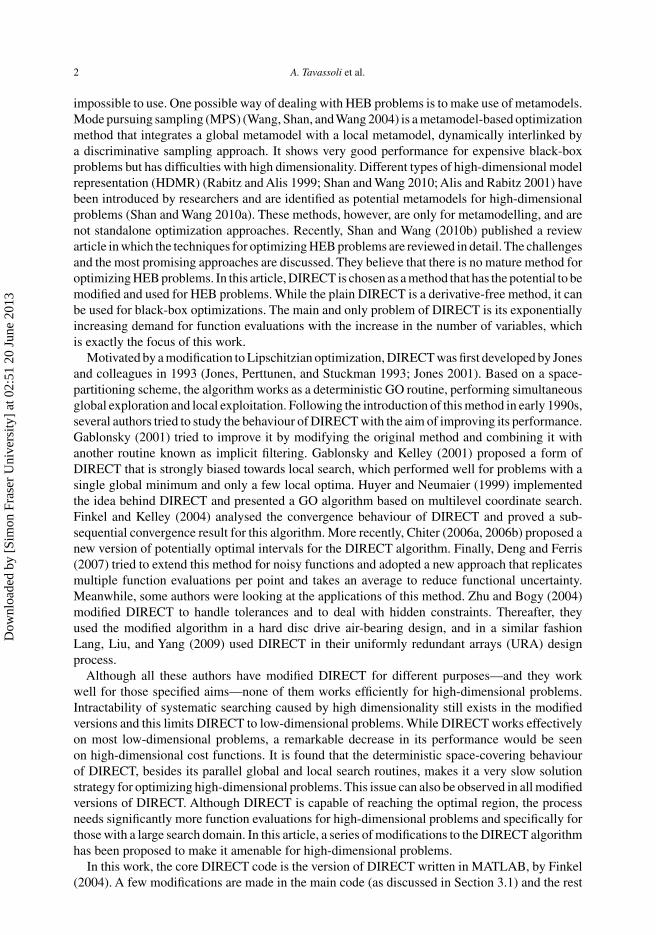
In each of the iterations, the potentially optimal hyperrectangle is being identified and par-titioned into a set of smaller domains, by trisecting it with respect to the longest coordinate itpossesses (Figure 1). The identification of a potentially optimal hyperrectangle would be basedon its size and the value of the objective function at its centre. Thus, potentially optimal hyper-rectangles either have low function values at their centres or are large enough to be good targetsfor global search. In other words, if α represents the size of the hyperrectangle, calculated asthe distance from the centre point to the corner point of the hyperrectangle, and assuming H asthe index set of existing hyperrectangles, a hyperrectangle i ∈ H is called a potentially optimalcandidate if there exists a constant ξ so that:

f (ci) − ξαi ≤ f (cj) − ξαj, ∀j ∈ H (2)

f (ci) − ξαi ≤ fmin − ε|fmin| (3)

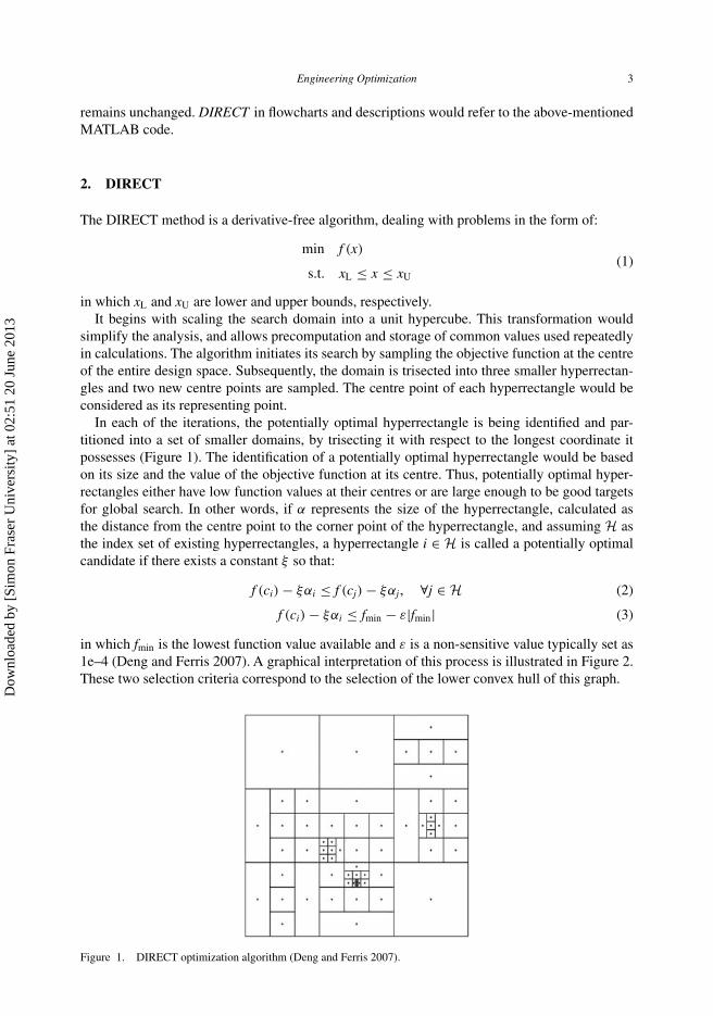
in which fmin is the lowest function value available and ε is a non-sensitive value typically set as1e–4 (Deng and Ferris 2007). A graphical interpretation of this process is illustrated in Figure 2.These two selection criteria correspond to the selection of the lower convex hull of this graph.

Figure 1. DIRECT optimization algorithm (Deng and Ferris 2007).

Dow

nloa

ded

by [

Sim

on F

rase

r U

nive

rsity

] at

02:

51 2

0 Ju

ne 2

013

4 A. Tavassoli et al.

Figure 2. Identifying the potentially optimal hyperrectangles (Deng and Ferris 2007).

Assuming an infinite number of iterations, DIRECT is proven to converge to the global optimumas long as the objective function is continuous or at least continuous in the neighbourhood of theglobal optimum. Readers are encouraged to see Jones, Perttunen, and Stuckman (1993) for acomprehensive description of DIRECT.

3. High-dimensional DIRECT

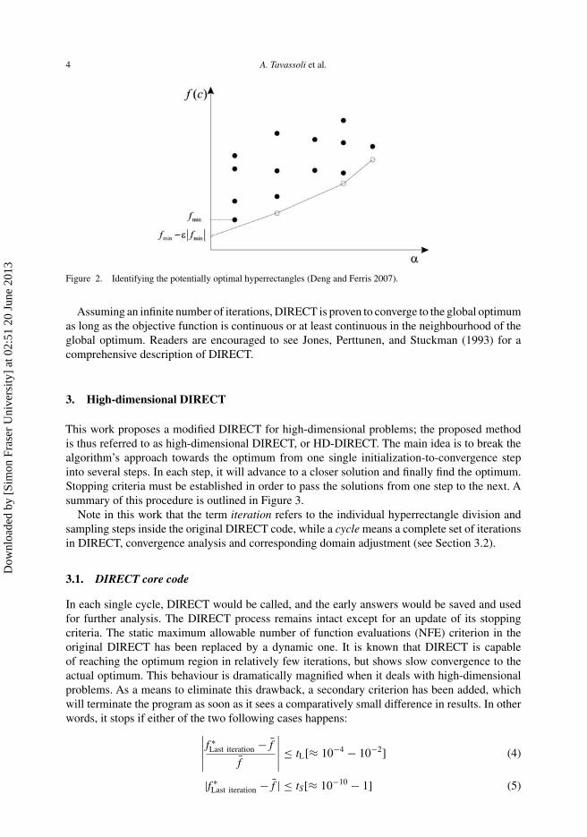
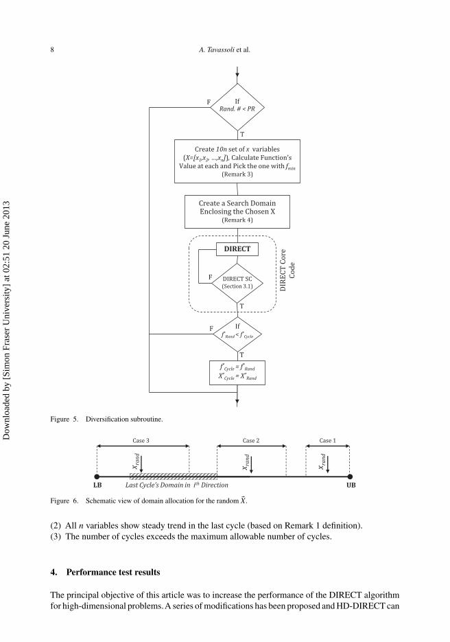
This work proposes a modified DIRECT for high-dimensional problems; the proposed methodis thus referred to as high-dimensional DIRECT, or HD-DIRECT. The main idea is to break thealgorithm’s approach towards the optimum from one single initialization-to-convergence stepinto several steps. In each step, it will advance to a closer solution and finally find the optimum.Stopping criteria must be established in order to pass the solutions from one step to the next. Asummary of this procedure is outlined in Figure 3.

Note in this work that the term iteration refers to the individual hyperrectangle division andsampling steps inside the original DIRECT code, while a cycle means a complete set of iterationsin DIRECT, convergence analysis and corresponding domain adjustment (see Section 3.2).

3.1. DIRECT core code

In each single cycle, DIRECT would be called, and the early answers would be saved and usedfor further analysis. The DIRECT process remains intact except for an update of its stoppingcriteria. The static maximum allowable number of function evaluations (NFE) criterion in theoriginal DIRECT has been replaced by a dynamic one. It is known that DIRECT is capableof reaching the optimum region in relatively few iterations, but shows slow convergence to theactual optimum. This behaviour is dramatically magnified when it deals with high-dimensionalproblems. As a means to eliminate this drawback, a secondary criterion has been added, whichwill terminate the program as soon as it sees a comparatively small difference in results. In otherwords, it stops if either of the two following cases happens:

∣∣∣∣∣f ∗Last iteration − f̄

f̄

∣∣∣∣∣ ≤ tL[≈ 10−4 − 10−2] (4)

|f ∗Last iteration − f̄ | ≤ tS[≈ 10−10 − 1] (5)

Dow

nloa

ded

by [

Sim

on F

rase

r U

nive

rsity

] at

02:

51 2

0 Ju

ne 2

013

Engineering Optimization 5

Figure 3. Flowchart of the high-dimensional-DIRECT algorithm.

in which

f ∗Last iteration = fi in the last iteration

f̄ = Average of fi in last 3–10 iterations

The averaging of function values is being done dynamically among the last three to 10 prioriterations, based on the number of cycles it has gone through. Evidently, early cycles need roughapproximation, while later ones will need higher accuracy. For the initial cycle, only three prioriterations are used for calculating the average f values. In the following cycles, this numbergradually increases by one at each cycle until reaching 10, which is then used for all ensuringcycles until convergence.

As mentioned earlier, the maximum allowable NFE will also change according to the progressof convergence. Starting with a relatively high value, it will change to 1.3 times the NFE in which

Dow

nloa

ded

by [

Sim

on F

rase

r U

nive

rsity

] at

02:

51 2

0 Ju

ne 2

013

6 A. Tavassoli et al.

the previous cycle has terminated. This criterion prevents DIRECT from wasting a large numberof NFE, while the factor of 1.3 ensures that the NFE will not approach an undesirable smallvalue, especially in the last cycles. DIRECT, including these two stopping criteria, will be calledDIRECT core code from now on.

3.2. Result analysis and domain reconstruction

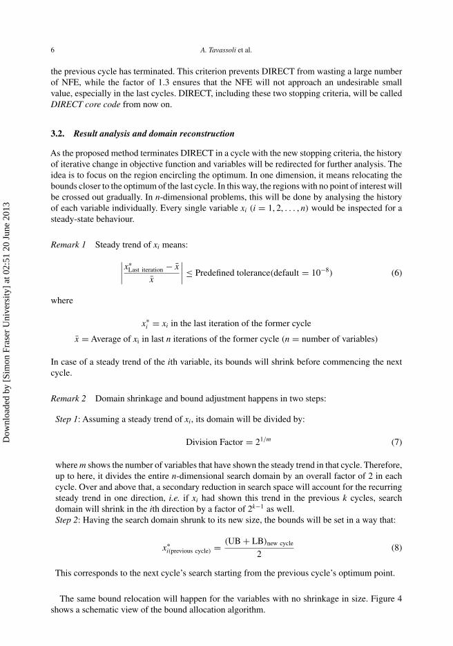
As the proposed method terminates DIRECT in a cycle with the new stopping criteria, the historyof iterative change in objective function and variables will be redirected for further analysis. Theidea is to focus on the region encircling the optimum. In one dimension, it means relocating thebounds closer to the optimum of the last cycle. In this way, the regions with no point of interest willbe crossed out gradually. In n-dimensional problems, this will be done by analysing the historyof each variable individually. Every single variable xi (i = 1, 2, . . . , n) would be inspected for asteady-state behaviour.

Remark 1 Steady trend of xi means:

∣∣∣∣x∗

Last iteration − x̄

x̄

∣∣∣∣ ≤ Predefined tolerance(default = 10−8) (6)

where

x∗i = xi in the last iteration of the former cycle

x̄ = Average of xi in last n iterations of the former cycle (n = number of variables)

In case of a steady trend of the ith variable, its bounds will shrink before commencing the nextcycle.

Remark 2 Domain shrinkage and bound adjustment happens in two steps:

Step 1: Assuming a steady trend of xi, its domain will be divided by:

Division Factor = 21/m (7)

where m shows the number of variables that have shown the steady trend in that cycle. Therefore,up to here, it divides the entire n-dimensional search domain by an overall factor of 2 in eachcycle. Over and above that, a secondary reduction in search space will account for the recurringsteady trend in one direction, i.e. if xi had shown this trend in the previous k cycles, searchdomain will shrink in the ith direction by a factor of 2k−1 as well.Step 2: Having the search domain shrunk to its new size, the bounds will be set in a way that:

x∗i(previous cycle) = (UB + LB)new cycle

2(8)

This corresponds to the next cycle’s search starting from the previous cycle’s optimum point.

The same bound relocation will happen for the variables with no shrinkage in size. Figure 4shows a schematic view of the bound allocation algorithm.

Dow

nloa

ded

by [

Sim

on F

rase

r U

nive

rsity

] at

02:

51 2

0 Ju

ne 2

013

Engineering Optimization 7

Figure 4. Schematic view of domain change with x∗ at the centre of the new space.

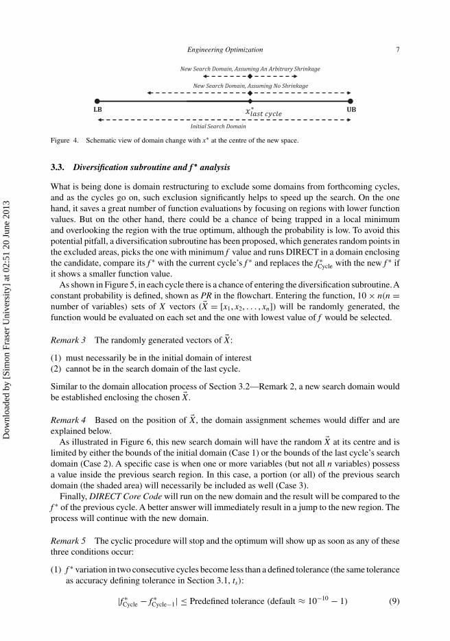
3.3. Diversification subroutine and f ∗ analysis

What is being done is domain restructuring to exclude some domains from forthcoming cycles,and as the cycles go on, such exclusion significantly helps to speed up the search. On the onehand, it saves a great number of function evaluations by focusing on regions with lower functionvalues. But on the other hand, there could be a chance of being trapped in a local minimumand overlooking the region with the true optimum, although the probability is low. To avoid thispotential pitfall, a diversification subroutine has been proposed, which generates random points inthe excluded areas, picks the one with minimum f value and runs DIRECT in a domain enclosingthe candidate, compare its f ∗ with the current cycle’s f ∗ and replaces the f ∗

Cycle with the new f ∗ ifit shows a smaller function value.

As shown in Figure 5, in each cycle there is a chance of entering the diversification subroutine.Aconstant probability is defined, shown as PR in the flowchart. Entering the function, 10 × n(n =number of variables) sets of X vectors (�X = [x1, x2, . . . , xn]) will be randomly generated, thefunction would be evaluated on each set and the one with lowest value of f would be selected.

Remark 3 The randomly generated vectors of �X:

(1) must necessarily be in the initial domain of interest(2) cannot be in the search domain of the last cycle.

Similar to the domain allocation process of Section 3.2—Remark 2, a new search domain wouldbe established enclosing the chosen �X .

Remark 4 Based on the position of �X , the domain assignment schemes would differ and areexplained below.

As illustrated in Figure 6, this new search domain will have the random �X at its centre and islimited by either the bounds of the initial domain (Case 1) or the bounds of the last cycle’s searchdomain (Case 2). A specific case is when one or more variables (but not all n variables) possessa value inside the previous search region. In this case, a portion (or all) of the previous searchdomain (the shaded area) will necessarily be included as well (Case 3).

Finally, DIRECT Core Code will run on the new domain and the result will be compared to thef ∗ of the previous cycle. A better answer will immediately result in a jump to the new region. Theprocess will continue with the new domain.

Remark 5 The cyclic procedure will stop and the optimum will show up as soon as any of thesethree conditions occur:

(1) f ∗ variation in two consecutive cycles become less than a defined tolerance (the same toleranceas accuracy defining tolerance in Section 3.1, ts):

|f ∗Cycle − f ∗

Cycle−1| ≤ Predefined tolerance (default ≈ 10−10 − 1) (9)

Dow

nloa

ded

by [

Sim

on F

rase

r U

nive

rsity

] at

02:

51 2

0 Ju

ne 2

013

8 A. Tavassoli et al.

Figure 5. Diversification subroutine.

Figure 6. Schematic view of domain allocation for the random �X .

(2) All n variables show steady trend in the last cycle (based on Remark 1 definition).(3) The number of cycles exceeds the maximum allowable number of cycles.

4. Performance test results

The principal objective of this article was to increase the performance of the DIRECT algorithmfor high-dimensional problems.A series of modifications has been proposed and HD-DIRECT can

Dow

nloa

ded

by [

Sim

on F

rase

r U

nive

rsity

] at

02:

51 2

0 Ju

ne 2

013

Engineering Optimization 9

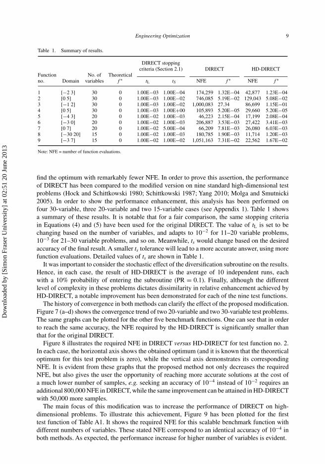
Table 1. Summary of results.

DIRECT stoppingcriteria (Section 2.1) DIRECT HD-DIRECT

Function No. of Theoreticalno. Domain variables f ∗ tL tS NFE f ∗ NFE f ∗

1 [−2 3] 30 0 1.00E−03 1.00E−04 174,259 1.32E−04 42,877 1.23E−042 [0 5] 30 0 1.00E−03 1.00E−02 746,085 5.19E−02 129,043 5.08E−023 [−1 2] 30 0 1.00E−03 1.00E−02 1,000,083 27.34 86,699 1.15E−014 [0 5] 30 0 1.00E−03 1.00E+00 105,893 5.20E−05 29,660 5.20E−055 [−4 3] 20 0 1.00E−02 1.00E−03 46,223 2.15E−04 17,199 2.08E−046 [−3 0] 20 0 1.00E−02 1.00E−03 206,887 3.53E−03 27,422 3.41E−037 [0 7] 20 0 1.00E−02 5.00E−04 66,209 7.81E−03 26,080 6.03E−038 [−30 20] 15 0 1.00E−02 1.00E−03 180,785 1.90E−03 11,714 1.20E−039 [−3 7] 15 0 1.00E−02 1.00E−02 1,051,163 7.31E−02 22,562 1.67E−02

Note: NFE = number of function evaluations.

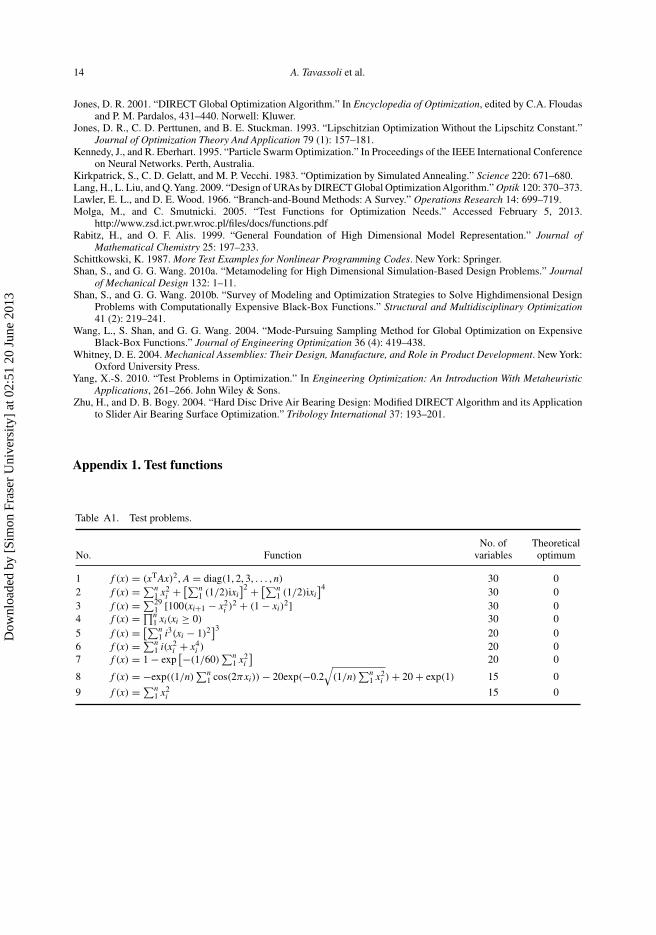
find the optimum with remarkably fewer NFE. In order to prove this assertion, the performanceof DIRECT has been compared to the modified version on nine standard high-dimensional testproblems (Hock and Schittkowski 1980; Schittkowski 1987; Yang 2010; Molga and Smutnicki2005). In order to show the performance enhancement, this analysis has been performed onfour 30-variable, three 20-variable and two 15-variable cases (see Appendix 1). Table 1 showsa summary of these results. It is notable that for a fair comparison, the same stopping criteriain Equations (4) and (5) have been used for the original DIRECT. The value of tL is set to bechanging based on the number of variables, and adapts to 10−2 for 11–20 variable problems,10−3 for 21–30 variable problems, and so on. Meanwhile, ts would change based on the desiredaccuracy of the final result. A smaller ts tolerance will lead to a more accurate answer, using morefunction evaluations. Detailed values of ts are shown in Table 1.

It was important to consider the stochastic effect of the diversification subroutine on the results.Hence, in each case, the result of HD-DIRECT is the average of 10 independent runs, eachwith a 10% probability of entering the subroutine (PR = 0.1). Finally, although the differentlevel of complexity in these problems dictates dissimilarity in relative enhancement achieved byHD-DIRECT, a notable improvement has been demonstrated for each of the nine test functions.

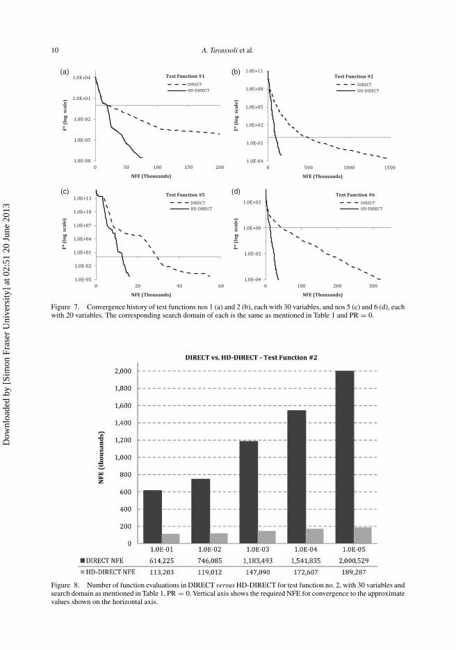
The history of convergence in both methods can clarify the effect of the proposed modification.Figure 7 (a–d) shows the convergence trend of two 20-variable and two 30-variable test problems.The same graphs can be plotted for the other five benchmark functions. One can see that in orderto reach the same accuracy, the NFE required by the HD-DIRECT is significantly smaller thanthat for the original DIRECT.

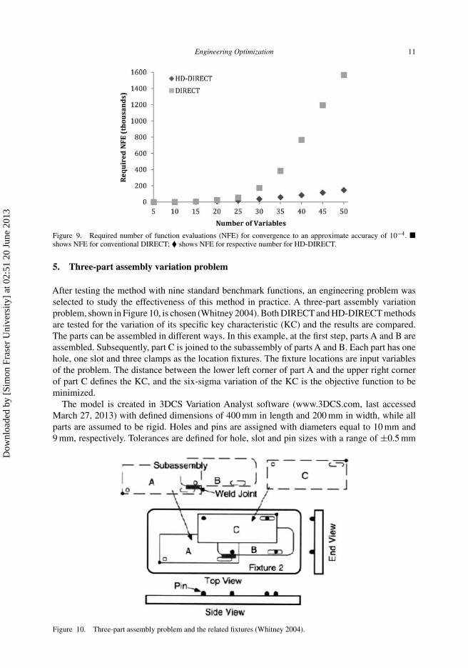
Figure 8 illustrates the required NFE in DIRECT versus HD-DIRECT for test function no. 2.In each case, the horizontal axis shows the obtained optimum (and it is known that the theoreticaloptimum for this test problem is zero), while the vertical axis demonstrates its correspondingNFE. It is evident from these graphs that the proposed method not only decreases the requiredNFE, but also gives the user the opportunity of reaching more accurate solutions at the cost ofa much lower number of samples, e.g. seeking an accuracy of 10−4 instead of 10−2 requires anadditional 800,000 NFE in DIRECT, while the same improvement can be attained in HD-DIRECTwith 50,000 more samples.

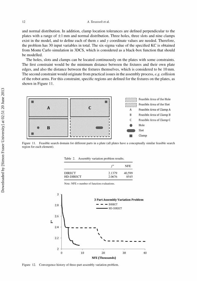
The main focus of this modification was to increase the performance of DIRECT on high-dimensional problems. To illustrate this achievement, Figure 9 has been plotted for the firsttest function of Table A1. It shows the required NFE for this scalable benchmark function withdifferent numbers of variables. These stated NFE correspond to an identical accuracy of 10−4 inboth methods. As expected, the performance increase for higher number of variables is evident.

Dow

nloa

ded

by [

Sim

on F

rase

r U

nive

rsity

] at

02:

51 2

0 Ju

ne 2

013

10 A. Tavassoli et al.

(a) (b)

(c) (d)

Figure 7. Convergence history of test functions nos 1 (a) and 2 (b), each with 30 variables, and nos 5 (c) and 6 (d), eachwith 20 variables. The corresponding search domain of each is the same as mentioned in Table 1 and PR = 0.

Figure 8. Number of function evaluations in DIRECT versus HD-DIRECT for test function no. 2, with 30 variables andsearch domain as mentioned in Table 1, PR = 0. Vertical axis shows the required NFE for convergence to the approximatevalues shown on the horizontal axis.

Dow

nloa

ded

by [

Sim

on F

rase

r U

nive

rsity

] at

02:

51 2

0 Ju

ne 2

013

Engineering Optimization 11

Figure 9. Required number of function evaluations (NFE) for convergence to an approximate accuracy of 10−4. �shows NFE for conventional DIRECT; � shows NFE for respective number for HD-DIRECT.

5. Three-part assembly variation problem

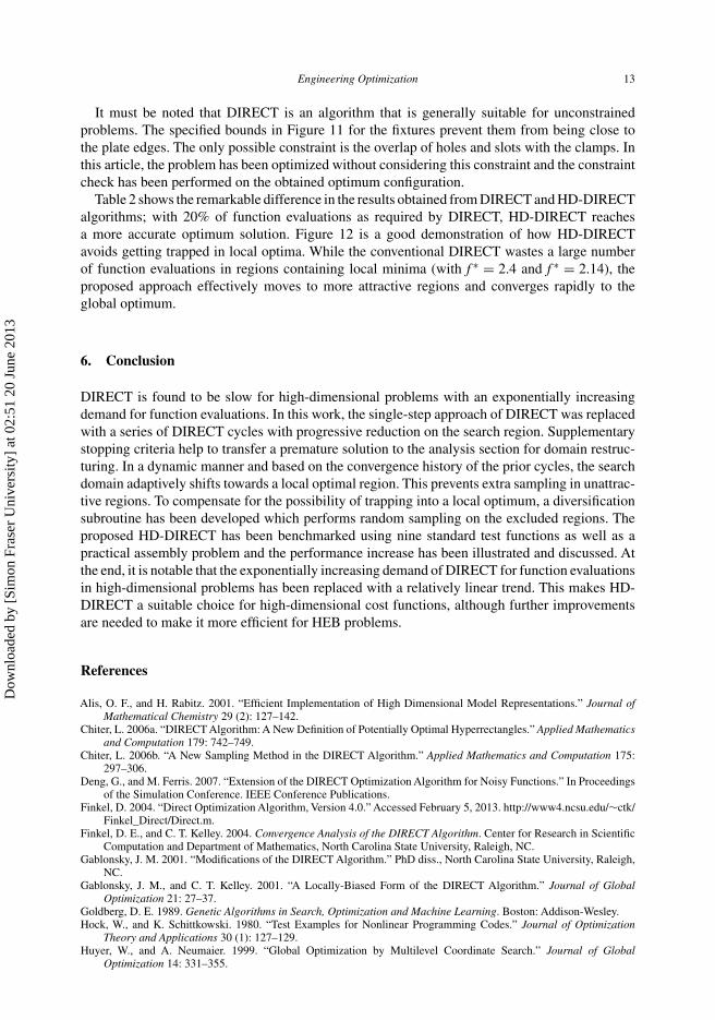
After testing the method with nine standard benchmark functions, an engineering problem wasselected to study the effectiveness of this method in practice. A three-part assembly variationproblem, shown in Figure 10, is chosen (Whitney 2004). Both DIRECT and HD-DIRECT methodsare tested for the variation of its specific key characteristic (KC) and the results are compared.The parts can be assembled in different ways. In this example, at the first step, parts A and B areassembled. Subsequently, part C is joined to the subassembly of parts A and B. Each part has onehole, one slot and three clamps as the location fixtures. The fixture locations are input variablesof the problem. The distance between the lower left corner of part A and the upper right cornerof part C defines the KC, and the six-sigma variation of the KC is the objective function to beminimized.

The model is created in 3DCS Variation Analyst software (www.3DCS.com, last accessedMarch 27, 2013) with defined dimensions of 400 mm in length and 200 mm in width, while allparts are assumed to be rigid. Holes and pins are assigned with diameters equal to 10 mm and9 mm, respectively. Tolerances are defined for hole, slot and pin sizes with a range of ±0.5 mm

Figure 10. Three-part assembly problem and the related fixtures (Whitney 2004).

Dow

nloa

ded

by [

Sim

on F

rase

r U

nive

rsity

] at

02:

51 2

0 Ju

ne 2

013

12 A. Tavassoli et al.

and normal distribution. In addition, clamp location tolerances are defined perpendicular to theplates with a range of ±1 mm and normal distribution. Three holes, three slots and nine clampsexist in the model, and to define each of them x and y coordinate values are needed. Therefore,the problem has 30 input variables in total. The six-sigma value of the specified KC is obtainedfrom Monte Carlo simulation in 3DCS, which is considered as a black-box function that shouldbe modelled.

The holes, slots and clamps can be located continuously on the plates with some constraints.The first constraint would be the minimum distance between the fixtures and their own plateedges, and also the distance between the fixtures themselves, which is considered to be 10 mm.The second constraint would originate from practical issues in the assembly process, e.g. collisionof the robot arms. For this constraint, specific regions are defined for the fixtures on the plates, asshown in Figure 11.

Figure 11. Feasible search domain for different parts in a plate (all plates have a conceptually similar feasible searchregion for each element).

Table 2. Assembly variation problem results.

f ∗ NFE

DIRECT 2.1379 40,599HD-DIRECT 2.0676 8545

Note: NFE = number of function evaluations.

Figure 12. Convergence history of three-part assembly variation problem.

Dow

nloa

ded

by [

Sim

on F

rase

r U

nive

rsity

] at

02:

51 2

0 Ju

ne 2

013

Engineering Optimization 13

It must be noted that DIRECT is an algorithm that is generally suitable for unconstrainedproblems. The specified bounds in Figure 11 for the fixtures prevent them from being close tothe plate edges. The only possible constraint is the overlap of holes and slots with the clamps. Inthis article, the problem has been optimized without considering this constraint and the constraintcheck has been performed on the obtained optimum configuration.

Table 2 shows the remarkable difference in the results obtained from DIRECT and HD-DIRECTalgorithms; with 20% of function evaluations as required by DIRECT, HD-DIRECT reachesa more accurate optimum solution. Figure 12 is a good demonstration of how HD-DIRECTavoids getting trapped in local optima. While the conventional DIRECT wastes a large numberof function evaluations in regions containing local minima (with f ∗ = 2.4 and f ∗ = 2.14), theproposed approach effectively moves to more attractive regions and converges rapidly to theglobal optimum.

6. Conclusion

DIRECT is found to be slow for high-dimensional problems with an exponentially increasingdemand for function evaluations. In this work, the single-step approach of DIRECT was replacedwith a series of DIRECT cycles with progressive reduction on the search region. Supplementarystopping criteria help to transfer a premature solution to the analysis section for domain restruc-turing. In a dynamic manner and based on the convergence history of the prior cycles, the searchdomain adaptively shifts towards a local optimal region. This prevents extra sampling in unattrac-tive regions. To compensate for the possibility of trapping into a local optimum, a diversificationsubroutine has been developed which performs random sampling on the excluded regions. Theproposed HD-DIRECT has been benchmarked using nine standard test functions as well as apractical assembly problem and the performance increase has been illustrated and discussed. Atthe end, it is notable that the exponentially increasing demand of DIRECT for function evaluationsin high-dimensional problems has been replaced with a relatively linear trend. This makes HD-DIRECT a suitable choice for high-dimensional cost functions, although further improvementsare needed to make it more efficient for HEB problems.

References

Alis, O. F., and H. Rabitz. 2001. “Efficient Implementation of High Dimensional Model Representations.” Journal ofMathematical Chemistry 29 (2): 127–142.

Chiter, L. 2006a. “DIRECT Algorithm: A New Definition of Potentially Optimal Hyperrectangles.” Applied Mathematicsand Computation 179: 742–749.

Chiter, L. 2006b. “A New Sampling Method in the DIRECT Algorithm.” Applied Mathematics and Computation 175:297–306.

Deng, G., and M. Ferris. 2007. “Extension of the DIRECT Optimization Algorithm for Noisy Functions.” In Proceedingsof the Simulation Conference. IEEE Conference Publications.

Finkel, D. 2004. “Direct Optimization Algorithm, Version 4.0.” Accessed February 5, 2013. http://www4.ncsu.edu/∼ctk/Finkel_Direct/Direct.m.

Finkel, D. E., and C. T. Kelley. 2004. Convergence Analysis of the DIRECT Algorithm. Center for Research in ScientificComputation and Department of Mathematics, North Carolina State University, Raleigh, NC.

Gablonsky, J. M. 2001. “Modifications of the DIRECT Algorithm.” PhD diss., North Carolina State University, Raleigh,NC.

Gablonsky, J. M., and C. T. Kelley. 2001. “A Locally-Biased Form of the DIRECT Algorithm.” Journal of GlobalOptimization 21: 27–37.

Goldberg, D. E. 1989. Genetic Algorithms in Search, Optimization and Machine Learning. Boston: Addison-Wesley.Hock, W., and K. Schittkowski. 1980. “Test Examples for Nonlinear Programming Codes.” Journal of Optimization

Theory and Applications 30 (1): 127–129.Huyer, W., and A. Neumaier. 1999. “Global Optimization by Multilevel Coordinate Search.” Journal of Global

Optimization 14: 331–355.

Dow

nloa

ded

by [

Sim

on F

rase

r U

nive

rsity

] at

02:

51 2

0 Ju

ne 2

013

14 A. Tavassoli et al.

Jones, D. R. 2001. “DIRECT Global Optimization Algorithm.” In Encyclopedia of Optimization, edited by C.A. Floudasand P. M. Pardalos, 431–440. Norwell: Kluwer.

Jones, D. R., C. D. Perttunen, and B. E. Stuckman. 1993. “Lipschitzian Optimization Without the Lipschitz Constant.”Journal of Optimization Theory And Application 79 (1): 157–181.

Kennedy, J., and R. Eberhart. 1995. “Particle Swarm Optimization.” In Proceedings of the IEEE International Conferenceon Neural Networks. Perth, Australia.

Kirkpatrick, S., C. D. Gelatt, and M. P. Vecchi. 1983. “Optimization by Simulated Annealing.” Science 220: 671–680.Lang, H., L. Liu, and Q.Yang. 2009. “Design of URAs by DIRECT Global Optimization Algorithm.” Optik 120: 370–373.Lawler, E. L., and D. E. Wood. 1966. “Branch-and-Bound Methods: A Survey.” Operations Research 14: 699–719.Molga, M., and C. Smutnicki. 2005. “Test Functions for Optimization Needs.” Accessed February 5, 2013.

http://www.zsd.ict.pwr.wroc.pl/files/docs/functions.pdfRabitz, H., and O. F. Alis. 1999. “General Foundation of High Dimensional Model Representation.” Journal of

Mathematical Chemistry 25: 197–233.Schittkowski, K. 1987. More Test Examples for Nonlinear Programming Codes. New York: Springer.Shan, S., and G. G. Wang. 2010a. “Metamodeling for High Dimensional Simulation-Based Design Problems.” Journal

of Mechanical Design 132: 1–11.Shan, S., and G. G. Wang. 2010b. “Survey of Modeling and Optimization Strategies to Solve Highdimensional Design

Problems with Computationally Expensive Black-Box Functions.” Structural and Multidisciplinary Optimization41 (2): 219–241.

Wang, L., S. Shan, and G. G. Wang. 2004. “Mode-Pursuing Sampling Method for Global Optimization on ExpensiveBlack-Box Functions.” Journal of Engineering Optimization 36 (4): 419–438.

Whitney, D. E. 2004. Mechanical Assemblies: Their Design, Manufacture, and Role in Product Development. New York:Oxford University Press.

Yang, X.-S. 2010. “Test Problems in Optimization.” In Engineering Optimization: An Introduction With MetaheuristicApplications, 261–266. John Wiley & Sons.

Zhu, H., and D. B. Bogy. 2004. “Hard Disc Drive Air Bearing Design: Modified DIRECT Algorithm and its Applicationto Slider Air Bearing Surface Optimization.” Tribology International 37: 193–201.

Appendix 1. Test functions

Table A1. Test problems.

No. of TheoreticalNo. Function variables optimum

1 f (x) = (xTAx)2, A = diag(1, 2, 3, . . . , n) 30 02 f (x) = ∑n

1 x2i + [∑n

1 (1/2)ixi]2 + [∑n

1 (1/2)ixi]4

30 03 f (x) = ∑29

1 [100(xi+1 − x2i )2 + (1 − xi)

2] 30 04 f (x) = ∏n

1 xi(xi ≥ 0) 30 05 f (x) = [∑n

1 i3(xi − 1)2]3

20 06 f (x) = ∑n

1 i(x2i + x4

i ) 20 07 f (x) = 1 − exp

[−(1/60)∑n

1 x2i

]20 0

8 f (x) = −exp((1/n)∑n

1 cos(2πxi)) − 20exp(−0.2√

(1/n)∑n

1 x2i ) + 20 + exp(1) 15 0

9 f (x) = ∑n1 x2

i 15 0

Dow

nloa

ded

by [

Sim

on F

rase

r U

nive

rsity

] at

02:

51 2

0 Ju

ne 2

013