Embed Size (px)
Citation preview
Master Thesis
(Projecte Final de Carrera)
Automatic Robust Classification of Speech Using Analytical
Feature Techniques
Gonçal Calvo i Pérez
Supervisors: Dr. François Pachet (Sony SCL Paris)
Dr. Antoni Bonafonte Cávez (UPC)
6, rue Amyot
75005 Paris
Escola Tècnica Superior d’Enginyeria de Telecomunicació de Barcelona
Universitat Politècnica de Catalunya
(ETSETB ‐ UPC)
January 2009


i
Abstract
This document reports the research done in the domain of automatic classification of speech within a Master’s degree internship in the Sony CSL laboratory. The work explores the potential of the EDS system, developed at Sony CSL, to solve speech recognition problems of a small number of isolated words, independently of the speaker, and with the presence of background noise. EDS automatically builds features for audio classification problems. This is done by means of (functional) composition of mathematical and signal processing operators. These features are called analytical features and are built by the system specifically for each audio classification problem, given under the form of a train and a test database.
In order to adapt EDS to speech classification, since features are generated through functional composition of basic operators, a research on specific operators for speech classification problems has been done, and new operators have been implemented and added to EDS. To test the performance of our approach to the problem, a speech database has been created, and experiments before and after adding the new specific operators have been carried out. An SVM classifier using EDS analytical features has then been compared to a standard HMM-based speech recognizer.
The results of the experiments indicate, on the one hand, that the new operators have shown to be useful to improve the speech classification performance. On the other hand, they show that EDS performs correctly in a speaker-dependent context, while further experimentation has to be done to draw conclusions in a speaker-independent situation.

iii
Resum
Aquest document és la memòria de la recerca efectuada dins del domini de la classificació automàtica de la parla durant una estada al laboratori Sony CSL per a la realització del projecte fi de carrera. El treball explora les possibilitats del sistema EDS, desenvolupat a Sony CSL, per resoldre problemes de reconeixement d’un petit nombre de mots aïllats, independentment del locutor i en presència de soroll de fons. EDS construeix automàticament features per problemes de classificació d’àudio. Això ho aconsegueix mitjançant la composició (funcional) d’operadors matemàtics i de processament de senyal. Per això aquestes features reben el nom de features analítiques, que el sistema construeix específicament per cada problema de classificació d’àudio, presentat sota la forma d’una base de dades d’entrenament i de test. Per tal d’adaptar EDS al reconeixement de la parla, com que les features són generades per mitjà de la composició funcional d’operadors bàsics, s’ha realitzat una recerca per trobar operadors específics per a problemes de classificació de veu, que s’han implementat i afegit a EDS. Per poder examinar els resultats de la nostra tècnica, s’ha creat una base de dades de veu, i s’han portat a terme una sèrie d’experiments abans i després d’haver afegit els nous operadors específics. Finalment un classificador SVM construït usant les features analítiques d’EDS ha estat comparat amb un sistema de reconeixement de veu basat en HMMs. Els resultats dels experiments indiquen, d’una banda, que els nous operadors s’han mostrat útils per reduir els errors de classificació de la parla. De l’altra, mostren que EDS funciona correctament en un context monolocutor, mentre que cal continuar la recerca per extreure conclusions definitives sobre les possibilitats d’EDS en entorns multilocutor.


v
Acknowledgements
With these words I want to thank all the people who have made this work possible.
First of all, the team which I worked with every day during the internship: my supervisor François Pachet, Pierre Roy (especially for the Java programming and debugging patience), Anthony Beurive (for his efficient C programming skills) and Amaury La Burthe and his always useful advices. I also wish to express my gratitude to my supervisor in the UPC, Antonio Bonafonte, for his very kind attention and help.
A big thanks to the people from who I received all their support: to Luc Steels, Sophie Boucher and the rest of the Sony CSL team; and to Carlos Agon and Fleur Gire, for being always there when I needed them, their patience and hospitality. I am also grateful to the public institutions that have organized and coordinated the ATIAM Master programme, from which this thesis was born: UPMC, TELECOM ParisTech and IRCAM; and of course to my engineering school, ETSETB.
I don’t forget the people that kindly contributed to the speech database: Gabriele Barbieri, Sophie Boucher, Amaury La Burthe, Nicolas Maisonneuve, Maria Niessen, Charlotte and François Pachet, Pierre Roy, Matthias Stevens, among others.
Finally, but not less important, a special “gràcies” to all the good friends I have made in Paris, to my family for their financial backing and love and to juDh, for her unconditional encouragement.

vii
Contents
List of Figures and Tables .................................................................................................................... ix
Abbreviations ........................................................................................................................................ x
1 Introduction ...................................................................................................................................... 1
1.1 Background ................................................................................................................................ 1
1.2 State of the Art in Speech Classification .................................................................................. 2
1.2.1 Speech Feature Extraction ................................................................................................... 3
1.2.2 State‐of‐the‐art Systems for Similar Problems .................................................................... 4
1.3 The Extractor Discovery System (EDS) ..................................................................................... 5
1.3.1 General Overview ................................................................................................................. 5
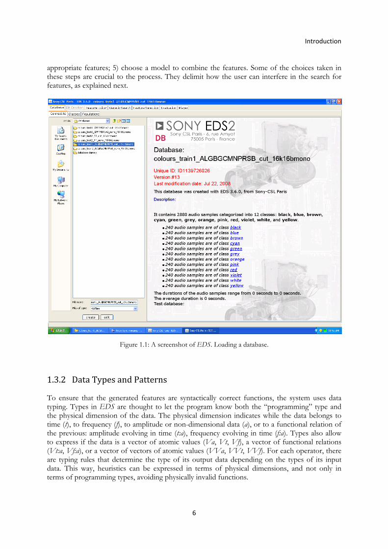
1.3.2 Data Types and Patterns ...................................................................................................... 6
1.3.3 Genetic Search ..................................................................................................................... 7
1.3.3.1 Genetic Operations ....................................................................................................... 8
1.3.3.2 Feature and Feature Set Evaluation .............................................................................. 9
1.3.4 Feature Selection ............................................................................................................... 11
1.3.5 Descriptor Creation and Evaluation ................................................................................... 12
1.4 Working Plan ........................................................................................................................... 13
1.5 Thesis Structure ....................................................................................................................... 14
2 Adapting EDS to Speech Classification .......................................................................................... 15
2.1 Classical Features for Speech Classification Problems ......................................................... 15
2.2 New Operators for EDS ........................................................................................................... 19
2.3 Limitations of EDS ................................................................................................................... 30
3 Experimental Work ........................................................................................................................ 33
3.1 The Databases .......................................................................................................................... 33
3.1.1 The Training Database ........................................................................................................ 33
viii
3.1.2 The Test Databases ............................................................................................................ 34
3.2 Pattern Sets .............................................................................................................................. 34
3.3 The First Experiment .............................................................................................................. 36
3.4 The Endpoint Detector ............................................................................................................ 37
3.5 The Experiments ...................................................................................................................... 39
3.5.1 Experiment with the Old Operators ................................................................................... 39
3.5.2 Experiment with the Old and New Operators ................................................................... 40
3.5.3 Experiment with the Old and New Operators and up to 35 Features ............................... 41
3.5.4 Experiment with an MFCC‐like Feature ............................................................................. 44
4 Discussion and Conclusions ........................................................................................................... 47
4.1 Results Discussion ................................................................................................................... 47
4.2 Comparison with a Standard Speech Classifier ..................................................................... 48
4.3 Conclusions .............................................................................................................................. 50
4.4 Future Work ............................................................................................................................. 51
Bibliography ........................................................................................................................................ 53
Appendices ........................................................................................................................................... 59
Appendix I – List of the EDS Operators .......................................................................................... 59
Appendix II – Results of the First Experiment .............................................................................. 61
Appendix III – Matlab® Code of the Endpoint Detector .............................................................. 64
Appendix IV – Results of the Experiment with the Old Operators .............................................. 70
Appendix V – Results of the Experiment with the Old and New Operators................................ 73
Appendix VI – Results of the Experiment with the Old and New Operators and up to 35 Features ............................................................................................................................................ 76
Appendix VII – Results of the Experiment with an MFCC‐like Feature ....................................... 79

ix
List of Figures and Tables
Figure 1.1: A screenshot of EDS. Loading a database ......................................................................... 6
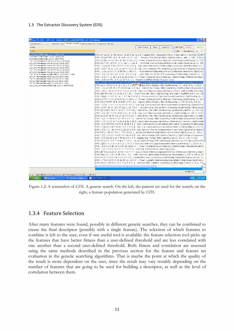
Figure 1.2: A screenshot of EDS. A genetic search ............................................................................ 11
Figure 1.3: A screenshot of EDS. The feature selector ...................................................................... 12
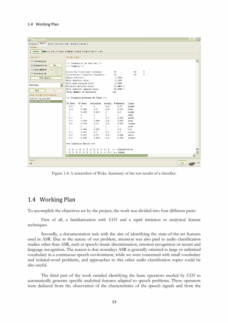
Figure 1.4: A screenshot of Weka. Summary of the test results of a classifier ............................... 13
Figure 2.1: CRRM gives higher values for voiced speech than for unvoiced speech ...................... 16
Figure 2.2: Waveforms of a signal before and after the application of AddWhiteNoise ................. 24
Figure 3.1: The endpoint detector applied to an utterance of the word white ............................... 37
Figure 3.2: The endpoint detector applied to an utterance of the word black ............................... 38
Figure 3.3: The endpoint detector applied to an utterance of the word blue ................................. 39
Figure 3.4: Evolution of the classification rates with the increase of the number of features used in an SVM classifier, for each test set .................................................................................... 43
Figure 4.1: Topology of the HMMs ..................................................................................................... 49
Table 4.1: Summary of all the main results ....................................................................................... 47
Table 4.2: Classification rate of the HMM‐based speech recogniser built with HTK and comparison with the results of the analytical feature + SVM technique ............................ 49

x
Abbreviations
ASR Automatic Speech Recognition AWGN Addtive White Gaussian Noise CMN Cepstral Mean Normalization DWCH Daubechies Wavelet Coefficient Histogram EDS Extractor Discovery System FFT Fast Fourier Transform HMM Hidden Markov Models HTK Hidden Markov Model Toolkit IFFT Inverse FFT LPC Linear Predictive Coding MFCC Mel-frequency cepstral coefficients RMS Root Mean Square SMO Sequential Minimal Optimization SNR Signal-to-Noise Ratio SVM Support Vector Machine ZCR Zero-Crossing Rate


1
Chapter 1
Introduction
1.1 Background
For its expansive possibilities and direct applications, Automatic Speech Recognition (ASR) has become an attractive domain of study in the area of information and communication technology for the last five decades. The challenge of building a machine capable to dialog with humans using natural language was in the mind of scientists for centuries, but it was not till the second half of the 20th century that technological advances made possible significant steps in that direction (Juang and Rabiner 2005). On the other hand, the increasing amount of information that generates today’s society has triggered off the need to create intelligent systems to automatically search, select and classify information. This interest has led to many developments in the data mining, information retrieval and pattern recognition domains. A key step to the success of classification problems is feature extraction. Features are the individual measurable heuristic properties of the phenomena being observed and, traditionally, construction and selection of good features has been made by hand. In the intersection of these two fields starts the idea of this work. Sony CSL is developing for some years the EDS (Extractor Discovery System), an original system for the automatic extraction of high-level audio descriptors, based on the idea of analytical feature (Zils and Pachet 2004; Pachet and Roy 2004). Conversely to the classical approach, these features, used for supervised classification, are invented by the system and are conceived for being particularly adapted to a specific problem, given under the form of a train and a test database. This approach has been shown promising for several examples of audio classification (Cabral et al. 2007) like urban sounds (Defréville et al. 2006), percussive sounds (Roy et al. 2007), or dog barks (Molnár et al. 2008). The aim of this work is to study how this technique can be applied to another type of sounds: short speech messages. The system should classify a small number of isolated messages, in a speaker-independent way, i.e. be able to identify the words uttered by subjects other than the ones the system was trained with. The system should be robust enough to work in non-ideal conditions, including the presence of background noise or voices of subjects of different ages and accents. Lastly, this speech classifier should work leaving aside sophisticated traditional techniques which use Hidden Markov Models (HMM).
Introduction
2
The hypothesis to verify through this work is that this new approach can be well-adapted to speech classification, but that new basic operators must be added to EDS to achieve good performances.
1.2 State of the Art in Speech Classification ASR technologies are present nowadays in infinity of applications used on a daily basis by millions of users, from GPS terminals to call centres, from weather information telephonic services to domestic speech-to-text software. Although automatic speech recognition and speech understanding systems are far from perfect in terms of accuracy, properly developed applications can still make good use of the existing technology to deliver real value to the costumer. Which are the state-of-the-art tools that make that possible? This is the question that we will try to answer in this section.
Juang and Rabiner (2005) revised the milestones in ASR research of the last four decades:
“In the 1960’s we were able to recognize small vocabularies (order of 10-100 words) of isolated words, based on simple acoustic-phonetic properties of speech sounds. The key technologies that were developed during this time frame were filter-bank analyses, simple time normalization methods, and the beginnings of sophisticated dynamic programming methodologies. In the 1970’s we were able to recognize medium vocabularies (order of 100-1000 words) using simple template-based, pattern recognition methods. The key technologies that were developed during this period were the pattern recognition models, the introduction of LPC methods for spectral representation, the pattern clustering methods for speaker-independent recognizers, and the introduction of dynamic programming methods for solving connected word recognition problems. In the 1980’s we started to tackle large vocabulary (1000-unlimited number of words) speech recognition problems based on statistical methods, with a wide range of networks for handling language structures. The key technologies introduced during this period were the hidden Markov model (HMM) and the stochastic language model, which together enabled powerful new methods for handling virtually any continuous speech recognition problem efficiently and with high performance. In the 1990’s we were able to build large vocabulary systems with unconstrained language models, and constrained task syntax models for continuous speech recognition and understanding. The key technologies developed during this period were the methods for stochastic language understanding, statistical learning of acoustic and language models, and the introduction of finite state transducer framework (and the FSM Library) and the methods for their determination and minimization for efficient implementation of large vocabulary speech understanding systems. Finally, in the last few years, we have seen the introduction of very large vocabulary systems with full semantic models, integrated with text-to-speech (TTS) synthesis systems, and multi-modal inputs (pointing, keyboards, mice, etc.). These systems enable spoken dialog systems with a range of input and output modalities for ease-of-use and flexibility in handling adverse environments where speech might not be as suitable as other input-output modalities. During this period we have seen the emergence of highly natural concatenative speech synthesis systems, the use of machine learning to improve both speech understanding and speech dialogs, and the introduction of mixed-initiative dialog systems to enable user control when necessary.”
1.2 State of the Art in Speech Classification
3
Despite the comercial exploitation of the ASR technologies is quite recent, major advances were brought about in the 1960’s and 1970’s via the introduction of advanced speech representations based on LPC analysis and cepstral analysis methods, and in the 1980’s through the introduction of rigorous statistical methods based on hidden Markov models. The main part of state-of-the-art speech feature extraction schemes are based on both LPC analysis (Hermansky 1990; Hermansky et al. 1991) and cepstral analysis (MFCC) (Acero and Huang 1995; Liu et al. 1993; Tyagi et al. 2003), while hidden Markov models have become the prevalent representation of speech units for speaker-independent continuous speech recognition (Holmes 1994).
1.2.1 Speech Feature Extraction In the feature extraction stage, since the speech signal is considered as a quasi-stationary process, speech analysis is performed on a short-term basis. Typically, the speech signal is divided into a number of overlapping time windows and a speech feature vector is computed to represent each of these frames. The size of the analysis window is usually of 20-30ms. The frame period is set to a value between 10 and 15ms.
The goal of front-end speech processing in ASR is to attain a projection of the speech signal to a compact parameter space where the information related to speech content can be extracted easily. Most parameterization schemes are developed based on the source-filter model of speech production mechanism. In this model, speech signal is considered as the output of a filter (vocal tract) whose input source is either glottal air pulses or random noise. For voiced sounds the glottal excitation is considered as a slowly varying periodic signal. This signal can be considered as the output of a glottal pulse filter feed with a periodic impulse train. For unvoiced sounds the excitation signal is considered as random noise.
State-of-the-art speech feature extraction schemes (Mel frequency cepstral coefficients
[Hunt et al. 1980] and perceptual linear prediction [Hermansky 1990]) are based on auditory processing on the spectrum of speech signal and cepstral representation of the resulting features. The spectral and cepstral analysis is generally performed using Fourier transform. The advantage of Fourier transform is that it possesses very good frequency localization properties.
Linear Predictive Coding has been considered one of the most powerful techniques
for speech analysis. LPC relies on the lossless tube model of the vocal tract. The lossless tube model approximates the instantaneous physiological shape of the the vocal tract as a concatenation of small cylindrical tubes. The model can be represented with an all pole (IIR) filter. LPC coefficients can be estimated using autocorrelation or covariance methods.
Cepstral analysis denote the unusual treatment of frequency domain data as it were time domain data. The cepstrum is a measure of the periodicity of a frequency response plot. The unit measure in cepstral domain is second but it indicates the variations in the frequency spectrum.
One of the powerful properties of cepstrum is the fact that any periodicities or repeated
patterns in a spectrum will be mapped to one or two specific components in the cepstrum. If a spectrum contains several harmonic series, they will be separated in a way similar to the way the spectrum separates repetitive time patterns in the waveform. The mel-frequency cepstral

Introduction
4
coefficients proposed by Mermelstein (Hunt et al. 1980) make use of this property to separate the excitation and vocal tract frequency components in cepstral domain. The spectrum of excitation signal is composed of several peaks at the harmonics of the pitch frequency. This constitutes the quickly varying component of the speech spectrum. On the other hand the vocal tract frequency response constitutes the slowly varying component of the speech spectrum. Hence a simple low pass liftering (i.e. filtering in cepstral domain) operation eliminates the excitation component.
As said in the beginning of this section, a feature vector is extracted for each frame. Typically, state-of-the-art recognition systems use feature vectors based on LPC or MFCC of length between 10 and 40. That means, that these systems need to extract between 1000 and 4000 values per second (with a usual frame period set to 10ms) from the speech signal (Bernal-Chaves et al. 2005).
1.2.2 State‐of‐the‐art Systems for Similar Problems ASR technologies face very different levels of complexity depending on the characteristics of the problem they are tackling. These problems can range from classifying a small size vocabulary of noise-free isolated words in a speaker-dependent context to recognize thousands of different words in a noisy continuous speech in speaker-independent situations.
In order to take some state-of-the-art solutions as a reference for the performances of our experiments, only systems that face similar problems to ours have to be taken into account. In particular, the characteristics that define our problem are the following:
• small vocabulary (10-20 words) • isolated words • speaker-independent context • presence of background noise
Research on systems thought to cope with problems of similar characteristics has being done for the last 30 years, and different performances have been reported depending on the proposed approach, though results are difficult to compare since they depend strongly on the database used in each experiment. For the same reason, a direct comparison of previous works with our system is not possible.
Rabiner and Wilpon (1979) reported a recognition accuracy of 95% on a classification problem with a moderate size vocabulary (54 words), using statistical clustering techniques to provide a set of word reference templates for a speaking-independent classifier, and dynamic time warping to align these templates with the tested words. Nevertheless, tests with subjects with foreign accents led to poor recognition accuracies of 50%.
More recently, the greatest advances have been achieved thanks to the development of complex statistical techniques based on hidden Markov models, though systems are still far from being perfect. These techniques were introduced because of the time dimension of the speech signal, which prevents to pose ASR as a simple static classification problem that could be solved using straightforward SVM classifiers using traditional feature vectors. In a problem with 10 classes of clean isolated words, Bernal-Chaves et al. (2005) reported a recognition accuracy of 99.67% of an HMM-based ASR system developed using the HTK package (Young et al. 2008)
1.3 The Extractor Discovery System (EDS)
5
that needed a 26 elements long feature vector every 10ms. These feature vectors were made of the MFCCs and energy of each signal frame. When the clean speech was corrupted with background noise (SNR = 12 dB), performances fell down up to accuracies of 33.36%.
The great majority of the state-of-the-art ASR systems are more or less complex variations of this last example, trying to solve robustness issues by improvements in the preprocessing of the speech signals, in the feature extraction stage or tuning better the HMMs.
Finally, it is important to note that, contrary to these traditional techniques, our approach
extracts only a feature vector per word (not one per signal frame), reducing notably the computational costs of the system and saving about 50 times more data storage (considering that the average word length is about 500ms). It does not use HMMs or dynamic time warping either, but a straightforward SVM classification algorithm. Thus, we want EDS to find features that are robust to time dealignments produced by different speaking speeds.
1.3 The Extractor Discovery System (EDS) The Extractor Discovery System started to be developed in 2003 thanks to the work of Aymeric Zils (Zils and Pachet 2004) at Sony CSL. As described by Cabral et al. (2007), the Extractor Discovery System is a heuristic-based generic approach for automatically extracting high-level audio descriptors from acoustic signals. EDS uses Genetic Programming (Koza 1992) to build extraction functions as compositions of basic mathematical and signal processing operators, such as Log, Variance, FFT, HanningWindow. A specific composition of such operators is called an analytical feature (e.g. Log (Variance (Min (FFT (Hanning (Signal)))))), and a combination of features forms a descriptor.
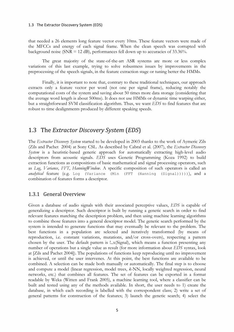
1.3.1 General Overview Given a database of audio signals with their associated perceptive values, EDS is capable of generalizing a descriptor. Such descriptor is built by running a genetic search in order to find relevant features matching the description problem, and then using machine learning algorithms to combine those features into a general descriptor model. The genetic search performed by the system is intended to generate functions that may eventually be relevant to the problem. The best functions in a population are selected and iteratively transformed (by means of reproduction, i.e. constant variations, mutations, and/or cross-overs), respecting a pattern chosen by the user. The default pattern is !_x(Signal), which means a function presenting any number of operations but a single value as result (for more information about EDS syntax, look at [Zils and Pachet 2004]). The populations of functions keep reproducing until no improvement is achieved, or until the user intervenes. At this point, the best functions are available to be combined. A selection can be made both manually or automatically. The final step is to choose and compute a model (linear regression, model trees, k-NN, locally weighted regression, neural networks, etc.) that combines all features. The set of features can be exported in a format readable by Weka (Witten and Frank 2005), a machine learning tool, where a classifier can be built and tested using any of the methods available. In short, the user needs to 1) create the database, in which each recording is labelled with the correspondent class; 2) write a set of general patterns for construction of the features; 3) launch the genetic search; 4) select the
Introduction
6
appropriate features; 5) choose a model to combine the features. Some of the choices taken in these steps are crucial to the process. They delimit how the user can interfere in the search for features, as explained next.
Figure 1.1: A screenshot of EDS. Loading a database.
1.3.2 Data Types and Patterns To ensure that the generated features are syntactically correct functions, the system uses data typing. Types in EDS are thought to let the program know both the “programming” type and the physical dimension of the data. The physical dimension indicates while the data belongs to time (t), to frequency (f), to amplitude or non-dimensional data (a), or to a functional relation of the previous: amplitude evolving in time (t:a), frequency evolving in time (f:a). Types also allow to express if the data is a vector of atomic values (Va, Vt, Vf), a vector of functional relations (Vt:a, Vf:a), or a vector of vectors of atomic values (VVa, VVt, VVf). For each operator, there are typing rules that determine the type of its output data depending on the types of its input data. This way, heuristics can be expressed in terms of physical dimensions, and not only in terms of programming types, avoiding physically invalid functions.

1.3 The Extractor Discovery System (EDS)
7
On the other hand, patterns are specified in the EDS algorithm in order to represent specific search strategies and guide the search of functions. The pattern encapsulates the architecture of the feature, and is a regular expression denoting subsets of features corresponding to a particular strategy for building them. Syntactically, it is expressed like an analytical feature, with the addition of regular expression operators, such as “!”, “?” and “*”. Patterns make use of types to specify the collections of targeted features in a generic way. More precisely:
• “?_τ” stands for one operator whose type is τ • “*_τ” stands for a composition of several operators whose types are all τ (for each of
them) • “!_τ” stands for several operators whose final type is τ (the types of the other operators
are arbitrary)
For example, the pattern: ?_a(!_Va(Split(*_t:a(x))))
can be instantiated by the following concrete analytical features:
Sum_a(Square_Va(Mean_Va(Split_Vt:a(HpFilter_t:a(x_t:a, 1000Hz), 100))))
Log10_a(Variance_a(Npeaks_Va(Split_Vt:a(Autocorrelation_t:a(x_t:a), 100), 10)))
1.3.3 Genetic Search Given a set of patterns, a genetic search is launched. It means that a population of features is created, and the capacity of each feature to separate (i.e. correctly classify) the samples in the training database is evaluated. The best features are selected as seeds for the next population. This process evolves the features until no improvement is found.
Although the genetic search can be performed fully automatically, the user can supervise
and interfere in the search. This intervention is even desired, since the space of possibilities is enormous, and heuristics are hard to express in most cases. Therefore, the user can lead the system through some specific paths by 1) stopping and restarting the search if it is following a bad path; 2) selecting specific features for future populations; 3) removing ineffective features from the search. Additionally, the stop condition itself is an important factor frequently left to the user.
The choice of the population size may also influence the search, since larger populations
may hold a bigger variety of features (which will converge slower), whereas smaller populations will perform a more in depth (faster) search (which will be most likely to terminate at local maxima). At last, the user can optimize features, finding the values for their arguments which maximize the class separation. For example, the split function (which divides a signal in sub-signals) has the size of the sub-signals as a parameter. Depending on the case, a tiny value can be notably better than large values, for example.
Introduction
8
1.3.3.1 Genetic Operations
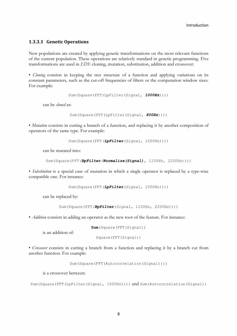
New populations are created by applying genetic transformations on the most relevant functions of the current population. These operations are relatively standard in genetic programming. Five transformations are used in EDS: cloning, mutation, substitution, addition and crossover: • Cloning consists in keeping the tree structure of a function and applying variations on its constant parameters, such as the cut-off frequencies of filters or the computation window sizes. For example:
Sum(Square(FFT(LpFilter(Signal, 1000Hz))))
can be cloned as:
Sum(Square(FFT(LpFilter(Signal, 800Hz))))
• Mutation consists in cutting a branch of a function, and replacing it by another composition of operators of the same type. For example:
Sum(Square(FFT(LpFilter(Signal, 1000Hz))))
can be mutated into:
Sum(Square(FFT(BpFilter(Normalize(Signal), 1100Hz, 2200Hz))))
• Substitution is a special case of mutation in which a single operator is replaced by a type-wise compatible one. For instance:
Sum(Square(FFT(LpFilter(Signal, 1000Hz))))
can be replaced by:
Sum(Square(FFT(BpFilter(Signal, 1100Hz, 2200Hz))))
• Addition consists in adding an operator as the new root of the feature. For instance:
Sum(Square(FFT(Signal)) is an addition of:
Square(FFT(Signal))
• Crossover consists in cutting a branch from a function and replacing it by a branch cut from another function. For example:
Sum(Square(FFT(Autocorrelation(Signal))))
is a crossover between: Sum(Square(FFT(LpFilter(Signal, 1000Hz)))) and Sum(Autocorrelation(Signal))
1.3 The Extractor Discovery System (EDS)
9
In addition to the genetically transformed functions, the new population is completed with a set of new randomly generated analytical features to ensure its diversity and introduce new operations in the population evolution.
1.3.3.2 Feature and Feature Set Evaluation
The evaluation of features is a delicate issue in feature generation. It is now well-known that good individual features do not necessarily form good feature sets when they are considered together (feature interaction). In principle, only feature sets should be considered during search, as there is no principled way to guarantee that a good individual feature will be good once it is in a given feature set. However, this induces a risk to narrow the search, as well as a high evaluation cost.
That is the reason why another option is chosen in EDS, based on our experiments with
large-scale feature generation, in which exploration of large areas of the analytical features’ space is favoured. Within a feature population, features are evaluated individually. Feature interaction is considered during the selection step for creating new populations.
Individual feature evaluation
There are several ways to assess the fitness of a feature. For classification problems, the Fischer Discriminant Ratio is often used because it is simple to compute and reliable for binary classification problems. However it is notoriously not adapted to multi-class problems, in particular for non convex distributions of data. To improve feature evaluation, a wrapper approach to feature selection has been chosen: features are evaluated using an SVM classifier built during the feature search with a 5-fold cross-validation on the training database. The fitness is the performance of the classifier built with this unique feature. As we often deal with multi-class classification (and not binary), the average F-measure is recommended to assess the classifier’s performance. However, as training databases are not necessarily balanced class-wise, the average F-measure can be artificially good. Therefore, the fitness in EDS is finally given by an F-measure vector (one F-measure per class) of the wrapper classifier. For regression problems, the Pearson correlation coefficient is used, but other methods could be applied, such as a wrapper approach with a regression SVM. Feature set evaluation: taking advantage of the syntactic form of analytical features
After a population has been created and each feature has been individually evaluated, a number of features need to be selected to be retained for the next population. In principle, such a feature selection process could be done using any feature selection algorithm, such as InfoGain. But feature selection algorithms usually require the computation of redundancy, which, in turn, implies the computation of correlations of feature’s values across samples. As our features are all analytical features, we take advantage of their syntactic expression to compute a rougher but efficient redundancy measure. This can be done thanks to the observation that syntactically similar analytical features have (statistically) correlated value series (Barbieri 2008). Additionally, our algorithm considers the performance of features on each class, and not globally for all classes.

Introduction
10
Finding an optimal solution would require a costly multi-criteria optimization. Instead, a low-complexity algorithm as a one-pass selection loop is proposed: we first select the best feature, and then iteratively select the next best feature not redundant with any of the selected ones, until we have the required number of features. Its particularity is to cycle through each class of the problem, and to take into account the redundancy between a feature and the currently built feature set using the syntactic structure of the feature. The algorithm is as follows:
FS {}; the feature set to build For each class C of the classification problem
S {non-selected features, sorted by decreasing performance wrt C}; For each feature F in S
If (F is not s-correlated to any feature in FS) FS FS + {F}; Break;
If (FS contains enough features) Return FS; Return FS;
The syntactic correlation (s-correlation) between 2 features is computed on the basis of their syntactic form. This not only speeds up the selection, but also forces the search algorithm to find features with a great diversity of operators. S-correlation is defined as a specific distance between two analytical features, using specific edit operations costs and taking into account analytical features’ types. More precisely, the cost of replacing operator Op1 by Op2 in an analytical feature is:
if Op1 = Op2 return 0 else if (Op1 != Op2) return 1
else return 2
In order to yield a Boolean s-correlation function, the edit distance for all pairs of features in the considered set (the analytical feature population in our case) is computed and the maximum (Max-s-distance) values for these distances are got. S-Correlation is finally defined as:
S-correlation (F, G): Return tree-edit-distance (f, g) >= ½ * Min-S-Correlation
As a consequence, our mechanism allows 1) to speed up the evaluation of individual features, thereby exploring a larger feature space, while 2) ensuring a syntactic diversity within feature populations.
1.3 The Extractor Discovery System (EDS)
11
Figure 1.2: A screenshot of EDS. A genetic search. On the left, the pattern set used for the search; on the right, a feature population generated by EDS.
1.3.4 Feature Selection After many features were found, possibly in different genetic searches, they can be combined to create the final descriptor (possibly with a single feature). The selection of which features to combine is left to the user, even if one useful tool is available: the feature selection tool picks up the features that have better fitness than a user-defined threshold and are less correlated with one another than a second user-defined threshold. Both fitness and correlation are assessed using the same methods described in the previous section for the feature and feature set evaluation in the genetic searching algorithms. That is maybe the point at which the quality of the result is more dependent on the user, since the result may vary notably depending on the number of features that are going to be used for building a descriptor, as well as the level of correlation between them.

Introduction
12
Figure 1.3: A screenshot of EDS. The feature selector.
1.3.5 Descriptor Creation and Evaluation Finally, in order to create a descriptor, the selected features must be exported to Weka, where a supervised learning method is chosen, and features are combined. The resultant descriptor is then evaluated on a test database, and Weka presents a summary with the results class per class, along with the precision rates.
1.4 Working Plan
13
Figure 1.4: A screenshot of Weka. Summary of the test results of a classifier.
1.4 Working Plan To accomplish the objectives set by the project, the work was divided into four different parts:
First of all, a familiarization with EDS and a rapid initiation to analytical feature techniques.
Secondly, a documentation task with the aim of identifying the state-of-the-art features used in ASR. Due to the nature of our problem, attention was also paid to audio classification studies other than ASR, such as speech/music discrimination, emotion recognition or accent and language recognition. The reason is that nowadays ASR is generally oriented to large or unlimited vocabulary in a continuous speech environment, while we were concerned with small vocabulary and isolated-word problems, and approaches to this other audio classification topics could be also useful.
The third part of the work entailed identifying the basic operators needed by EDS to
automatically generate specific analytical features adapted to speech problems. These operators were deduced from the observation of the characteristics of the speech signals and from the
Introduction
14
classical features identified in the previous stage. At this point, all the identified missing operators were implemented in EDS.
Finally, a series of experiments were carried out on a previously built database to test the
performance of EDS before and after adding the new basic operators to the system. Taking the features with best fitness that EDS had generated based on a training data base, some classifiers were built using Weka and were tested in various test sets. The last part of the work was analysing the results, comparing them to those obtained with a standard system, and proposing future work from the conclusions drawn.
1.5 Thesis Structure This work has been divided into four chapters: Chapter 1 introduces the framework in which the thesis has been developed. First, the state of the art in automatic speech recognition is presented, and then the EDS system is described.
Chapter 2 presents, first, the most relevant features used in speech recognition and other related domains. Next, it describes the 23 new EDS operators that have been designed in order to adapt EDS to speech classification, taking into account the features previously introduced. Finally, the last section describes the limitations of the system that have been found when carrying out this adaptation.
Chapter 3 contains the experimental work of the thesis. It presents the database used in
the experiments, along with an endpoint detector designed for cleaning the samples. It also describes the most interesting experiments that were carried out in order to study the performance of our approach, with and without the new operators.
Chapter 4 makes a summary and discusses the results obtained in the experiments. Then,
a comparison between our approach and a standard speech classifier is offered. Finally, the most important conclusions are extracted, and future work directions are suggested.
15
Chapter 2
Adapting EDS to Speech Classification
As described in the previous chapter, EDS builds new analytical features adapted to a specific problem, given under the form of a train and a test database. The construction of these features is made by means of the composition of basic operators.
The key issue of the work, discussed in this chapter, is finding the basic operators that must be added to the existing set of operators of EDS so that the system is able to produce good analytical features for speech classification problems. For this purpose, an extensive bibliographic research on ASR and other audio classification and recognition problems has been done to identify the features used classically (see next Section 2.1). For each feature in Section 2.1, it has been studied if EDS would be able to build it by means of the composition of the pre-existent operators. When that has been considered not possible, new operators have been described. Section 2.2 contains the description of the 23 new operators that have been implemented to EDS After the implementation of the additional operators, EDS is able to reach the features used classically if they are appropriate for the given problem. Moreover, it is able to improve their performance by applying to them genetic modifications, discovering new features well adapted to the problem. On the other hand, due to the particular characteristics of EDS, certain features can not be built with this approach. Section 2.3 explains the limitations of this analytical feature technique.
2.1 Classical Features for Speech Classification Problems There exists an extensive literature that discusses about features used in speech recognition. Next, there is a list of the most interesting ones that can contribute to the definition of specific operators for speech classification problems. A brief comment accompanies the feature when necessary. Since is not the aim of this document to give a deep description of these features, there is a bibliographic reference next to them to know more about their characteristics.
Adapting EDS to Speech Classification
16
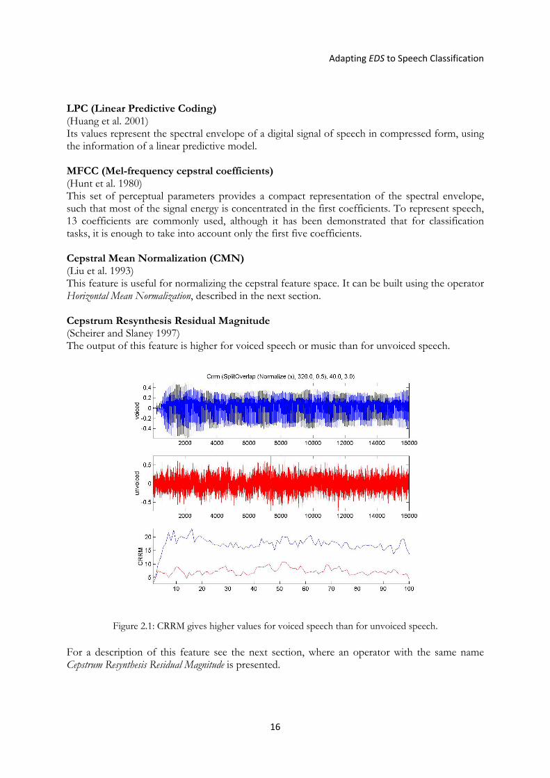
LPC (Linear Predictive Coding) (Huang et al. 2001) Its values represent the spectral envelope of a digital signal of speech in compressed form, using the information of a linear predictive model. MFCC (Mel-frequency cepstral coefficients) (Hunt et al. 1980) This set of perceptual parameters provides a compact representation of the spectral envelope, such that most of the signal energy is concentrated in the first coefficients. To represent speech, 13 coefficients are commonly used, although it has been demonstrated that for classification tasks, it is enough to take into account only the first five coefficients. Cepstral Mean Normalization (CMN) (Liu et al. 1993) This feature is useful for normalizing the cepstral feature space. It can be built using the operator Horizontal Mean Normalization, described in the next section. Cepstrum Resynthesis Residual Magnitude (Scheirer and Slaney 1997) The output of this feature is higher for voiced speech or music than for unvoiced speech.
Figure 2.1: CRRM gives higher values for voiced speech than for unvoiced speech. For a description of this feature see the next section, where an operator with the same name Cepstrum Resynthesis Residual Magnitude is presented.

2.1 Classical Features for Speech Classification Problems
17
Spectral Flux (Scheirer and Slaney 1997) The output of this feature, also known as Delta Spectrum Magnitude, is associated with the amount of spectral local changes. It is lower for speech, particularly voiced speech, than it is for music or unvoiced speech. The Spectral Flux is defined as the 2-norm of the frame-to-frame spectral amplitude difference vector, | | | | . Percentage of “Low-Energy” Frames (Scheirer and Slaney 1997) This measure will be higher for unvoiced speech than for voiced speech or music. It represents the proportion of frames with RMS power less than 50% of the mean RMS power within a one-second window. Spectral Centroid (Scheirer and Slaney 1997) This measure gives different results for voiced and unvoiced speech. It can be associated with the measure of brightness of a sound, and is obtained by evaluating the center of gravity of the spectrum:
∑ | |∑ | |
where represents the k-th frequency bin of the spectrum at frame t, and N is the number of frame samples. Spectral Roll-off Point (Scheirer and Slaney 1997) This measure will be higher for unvoiced speech than for voiced speech or music. It is the n-th percentile of the power spectral distribution, giving the frequency bin below which an n% of the magnitude distribution is concentrated. The feature gives an idea of the shape of the spectrum. Zero-Crossing Rate (ZCR) (Scheirer and Slaney 1997) This feature takes higher values for noise and unvoiced speech than for voiced speech. It is the number of time-domain zero-crossings within a speech frame. High Zero Crossing Rate Ratio (Alexandre et al. 2006) It takes higher values for speech than for music since speech is usually composed by alternating voiced and unvoiced fragments. This feature, computed from the ZCR, is defined as the number of frames whose ZCR is 1.5 times above the mean ZCR on a window containing M frames. Low Short-Time Energy Ratio (Alexandre et al. 2006) This measure will be higher for unvoiced speech than for voiced speech or music. Similarly to the High Zero Crossing Rate Ratio, it is obtained from the Short-Time Energy (i.e. the mean energy of the signal within each analysis frame), and defined as the ratio of frames whose Short-Time Energy is 0.5 times below the mean Short-Time Energy on a window that contains M frames.
Adapting EDS to Speech Classification
18
Standard Deviation of the Spectral Centroid + AWGN (Minematsu et al. 2006) The addition of white Gaussian noise (AWGN) only increases (slightly) the centroid value of the unvoiced segments. More generally, the addition of white Gaussian noise helps to reduce speaker differences in speech. Voicing Rate (Kitaoka et al. 2002) It gives higher values for segments of voiced speech than for unvoiced speech. This feature can be calculated as follows:
log
where is a sequence of LPC residual errors. An LPC model smoothes the spectral fine structure and the LPC residual error contains this information. This corresponds to the vibration of the glottal source. Normalized Pitch (Kitaoka et al. 2002) It normalizes the pitch, smoothing speaker-dependent variations. It is defined as:
,1
where is a sequence of log fundamental frequencies and N is the length of . Pitch Regression Coefficients (Kitaoka et al. 2002) Another way to reduce the speaker-dependent factor present in the pitch:
∆∑∑
where represents the log fundamental frequency and K is the window length to calculate the coefficients. Power Regression Coefficients (Kitaoka et al. 2002) It normalizes the power values, smoothing speaker-dependent and environment variations. This feature is calculated using the same formula as in Pitch Regression Coefficients, where represents, in this case, power (i.e. the logarithm of the square sum of the speech waveform). Delta MFCC (Deemagarn and Kawtrakul 2004) It measures the change in MFCC over time, in terms of velocity. This feature can be calculated using the same formula as in Pitch Regression Coefficients, where represents, in this case, the MFCC.
2.2 New Operators for EDS
19
Delta-Delta MFCC (Deemagarn and Kawtrakul 2004) It measures the change in MFCC over time, as well. It gives information about the acceleration of the coefficients. This second-order delta MFCC is usually defined from the first-order one as:
∆∆ ∆ ∆
Some operators can also act as signal preprocessing functions when they are placed in the
beginning of the chain of operators in an analytical feature. Apart from the well-known normalization and windowing functions, here they are some other usual ones for speech: High-Frequency Preemphasis (Nossair 1995) This tends to whiten the speech spectrum as well as emphasizing those frequencies to which the human auditory system is most sensitive. For a description of this filter see the next section, where an operator with the same name High-Frequency Preemphasis is presented. 2 kHz cut-off Low-Pass Filtering (Minematsu et al. 2006) It smoothes inter-speaker differences. It consists of applying a common low-pass filter to the signal, with a cut-off frequency of 2 kHz.
2.2 New Operators for EDS
A total of 23 new operators have been implemented in EDS. Most of them have appeared trying to adapt ideas of the classical features described in the previous section. In some cases, some of these classical features have become basic operators themselves due to the technical impossibility of building them through the composition of several simpler operators. Other operators – the horizontal ones – have been created after the observation of how EDS works, trying to cope with some typing characteristics inherent in the system. In the following lines, there is the description of the new operators. Some remarks:
• The names of the operators used in the EDS interface appear in brackets next to the operator’s name.
• The input arguments are also specified, and their default value and possible range are indicated whenever they are a parameter, following this format: (default value [min. value, max. value]).
• At the end of each description, there are the typing rules followed by EDS with the operator.
Horizontal Sum (HSum) arguments: input matrix It returns a matrix which elements are the sums of the rows of the input matrix.

Adapting EDS to Speech Classification
20
For each row of the input matrix, … , it returns the single value:
HSum is the analogue operator of the existing Sum for the computation by rows. Typing rules: atom_1 > NULL F?any_1:?any_2 > NULL! VF?any_1:?any_2 > Fany_1:any_2! V?atom_1 > NULL VV?atom_1 > Vatom_1 Norm (Norm) arguments: input matrix It returns a matrix which elements are the norms of the columns of the input matrix. For each column of the input matrix, … , it returns the single value:
Although EDS could find this result with the composition Sqrt (Sum (Power (x, 2))), Norm has been implemented since it is a frequently used basic operation. This is an operator associated with the energy of the input signal. Typing rules: atom_1 > NULL F?any_1:?any_2 > any_2 VF?any_1:?any_2 > Vany_2! V?atom_1 > atom_1 VV?atom_1 > Vatom_1 Horizontal Norm (HNorm) arguments: input matrix It returns a matrix which elements are the norms of the rows of the input matrix. For each row of the input matrix, … , it returns the single value:
HNorm is the analogue operator of Norm for the computation by rows. EDS can also reach it by doing Sqrt (HSum (Power (x, 2))) but, like Norm, it has been implemented to simplify its construction. This is an operator associated with the energy of the signal. Typing rules: atom_1 > NULL F?any_1:?any_2 > NULL! VF?any_1:?any_2 > Fany_1:any_2! V?atom_1 > NULL
2.2 New Operators for EDS
21
VV?atom_1 > Vatom_1 Horizontal Root Mean Square (HRms) arguments: input matrix It returns a matrix which elements are the RMS of the rows of the input matrix. For each row of the input matrix, … , it returns the single value:
HRms is the analogue operator of the existing Rms for the computation by rows. This is an operator associated with the power of the input signal. Typing rules: atom_1 > NULL F?any_1:?any_2 > NULL! VF?any_1:?any_2 > Fany_1:any_2! V?atom_1 > NULL VV?atom_1 > Vatom_1 Horizontal Percentile (HPercentile) arguments: input matrix, percentage (50 [1, 100]) It returns a column matrix where each row element is greater than a constant percentage (between 0 and 100) of the elements in the corresponding row of the input matrix. HPercentile is the analogue operator of the existing Percentile for the computation by rows. Typing rules: atom_1, n > NULL F?any_1:?any_2, n > NULL! VF?any_1:?any_2, n > Fany_1:any_2! V?atom_1, n > NULL VV?atom_1, n > Vatom_1 Horizontal Derivation (HDerivation) arguments: input matrix It returns a matrix which rows are the first derivative of the rows of the input matrix. For each row of the input matrix, … , it returns the vector:
… … 0
HDerivation is the analogue operator of the existing Derivation for the computation by rows. It is useful to compute the Spectral Flux, which can be computed in EDS as:
HNorm(HDerivation(Fft(SplitOverlap(x, window_size, overlap_percent))))
And for computing an approximation of the Delta and Delta-Delta MFCCs:

Adapting EDS to Speech Classification
22
HDerivation(Mfcc(SplitOverlap(x, window_size, overlap_percent),
number_coeffs)) HDerivation(HDerivation(Mfcc(SplitOverlap(x, window_size, overlap_percent),
number_coeffs))) Typing rules: V?atom_1 > NULL F?atom_1:?atom_2 > NULL VF?atom_1:?atom_2 > VFatom_1:atom_2 VV?atom_1 > VVatom_1 Horizontal Regression Coefficients (RegressionCoeffs) arguments: input matrix, regression order (1 [1, 3]) It returns a matrix which rows are the regression coefficients of the rows of the input matrix. For each row of the input matrix, , it returns the vector:
∆∑ ∑ ∀
The regression order K is a parameter that varies usually between 1 and 3. This operator is similar to HDerivation, and is very useful for capturing temporal information. If its input matrix is a matrix of MFCCs, we obtain the Delta MFCCs. In the syntax of EDS: RegressionCoeffs(Mfcc(SplitOverlap(x, 20ms, 50%), num_coeffs), reg_order)
Typing rules: V?atom_1, n > NULL F?atom_1:?atom_2, n > NULL VF?atom_1:?atom_2, n > VFatom_1:atom_2 VV?atom_1, n > VVatom_1 Vertical Regression Coefficients (VRegressionCoeffs) arguments: input matrix, regression order (1 [1, 3]) It returns a matrix which columns are the regression coefficients of the columns of the input matrix. VRegressionCoeffs is the analogue operator of RegressionCoeffs for the computation by columns. Thus, the formula is applied this time to each column of the input matrix. Similar to Derivation, this is a very useful operator for capturing temporal information. If the input matrix is a matrix of powers or pitches, we obtain the power and pitch regression coefficients. In the syntax of EDS:
VRegressionCoeffs(Log10(Norm(SplitOverlap(Normalize(x), 20ms, 50%))), reg_order)
VRegressionCoeffs(Pitch(SplitOverlap(x, 20ms, 50%))), reg_order) Typing rules: V?atom_1, n > Vatom_1 F?atom_1:?atom_2, n > Fatom_1:atom_2 VF?atom_1:?atom_2, n > VFatom_1:atom_2

2.2 New Operators for EDS
23
VV?atom_1, n > VVatom_1 Horizontal Mean Normalization (HMeanNormalization) arguments: input matrix It returns a matrix where each element is the corresponding element of the input matrix minus the average value of the corresponding row. Let’s call A the input matrix that contains N column vectors. A mean is computed for all the elements of each row of the input matrix, obtaining a column vector of means, let’s call it B. That is: · ∀ i Then, all the elements of each row of the input matrix are subtracted by their corresponding mean of the column vector, obtaining the normalised values in C:
∀ i, j This operator is useful to compute the Cepstral Mean Normalization, which is the Horizontal Mean Normalization when the input matrix is made of MFCC column vectors. In the syntax of EDS:
HMeanNormalization(Mfcc(SplitOverlap(x, 20ms, 50%), num_coeffs)) It is also useful in Normalised Formants, if the input matrix is a matrix of formants:
HMeanNormalization(FormantSplitPraat(x)) Typing rules: VV?any_1 > VVany_1! VF?any_1:?any_2 > VFany_1:any_2! Vertical Mean Normalization (VMeanNormalization) arguments: input matrix It returns a matrix where each element is the corresponding element of the input matrix minus the average value of the corresponding column. VMeanNormalization is the analogue operator of HMeanNormalization for the computation by columns. This operator is useful to compute the Normalised Pitch:
VMeanNormalization(Pitch(SplitOverlap(x, 20ms, 50%))) VMeanNormalization(PitchSplitPraat(x))
Typing rules: V?atom_1 > Vatom_1! F?atom_1:?atom_2 > Fatom_1:atom_2! VV?atom_1 > VVatom_1! VF?atom_1:?atom_2 > VFatom_1:atom_2!
Adapting EDS to Speech Classification
24
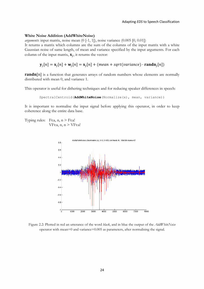
White Noise Addition (AddWhiteNoise) arguments: input matrix, noise mean (0 [-1, 1]), noise variance (0.005 [0, 0.01]) It returns a matrix which columns are the sum of the columns of the input matrix with a white Gaussian noise of same length, of mean and variance specified by the input arguments. For each column of the input matrix, , it returns the vector:
· n is a function that generates arrays of random numbers whose elements are normally
distributed with mean 0, and variance 1.
This operator is useful for dithering techniques and for reducing speaker differences in speech:
SpectralCentroid(AddWhiteNoise(Normalize(x), mean, variance)) It is important to normalise the input signal before applying this operator, in order to keep coherence along the entire data base. Typing rules: Ft:a, n, n > Ft:a! VFt:a, n, n > VFt:a!
Figure 2.2: Plotted in red an utterance of the word black, and in blue the output of the AddWhiteNoise operator with mean=0 and variance=0.005 as parameters, after normalising the signal.
2.2 New Operators for EDS
25
High-Frequency Preemphasis (HFPreemphasis) arguments: input matrix, preemphasis coefficient (0.97 [0.9, 1]) It returns a matrix which columns are the result of filtering the columns of the input matrix with a second-order FIR filter which two elements are [1 -precoeff]. For each column of the input matrix, , it returns the vector:
· 1 The relation between precoeff and the preemphasis frequency is:
·
Thus, the preemphasis coefficient depends on the sampling frequency. For around 16 kHz it is between 0.9 and 1, and usually between 0.95 and 0.98, yielding a cut-off frequency between 50 and 130 Hz. Typing rules: Ft:a, n > Ft:a! VFt:a, n > VFt:a! Cepstrum Resynthesis Residual Magnitude (Crrm) arguments: input matrix, number of mel band filters (27 [2, 40]), order of the smoothing filter (3 [2, 10]). It returns a matrix which contains the Cepstrum Resynthesis Residual Magnitude (CRRM) of the input matrix, taken as a temporal signal. The CRRM is defined as the norm of the difference between the magnitude of its spectrum and the magnitude of the same spectrum smoothed in the MFCC domain, both in the mel scale, i.e.:
where X[k] is the magnitude of the input signal’s spectrum in the Mel scale and Y[k] is the magnitude of the same spectrum smoothed in the Mel Frequency Cepstral Coefficients (MFCC) domain, also in the mel scale. In more detail, Y[k] is obtained first by calculating the MFCC of the input matrix, using as many mel band filters as in X[k], and then applying a moving average in order to smooth the results before returning to the spectral domain by applying the inverse Discrete Cosine Transform (iDCT) and taking its exponential. These two last operations are the inverse operations used in the computation of the MFCC, the DCT and the natural logarithm. The moving average of Nth order (normally order 2 or 3) is the convolution of its input vector with a vector of N+1 components and constant value , for 0, 1, … , . Typing rules: ?atom_1, n, n > NULL! F?atom_1:?atom_2, n, n > atom_2! VF?atom_1:?atom_2, n, n > Vatom_2! V?atom_1, n, n > atom_1! VV?atom_1, n, n > Vatom_1!
Adapting EDS to Speech Classification
26
Mel-Filterbank (MelFilterBank) arguments: input matrix, number of bands (10 [2, 40]) It returns a matrix which columns contain copies of the input matrix filtered through different mel-frequency bands. It uses a modified implementation of the yet existing FilterBank, where calculated filter bandwidths are passed as an argument to the modified FilterBank function. All the filters have the same bandwidth in the mel-frequency scale, and frequency scale values can be calculated using:
700 · .⁄ 1
Typing rules: F?atom_1:?atom_2, n > VFatom_1:atom_2! V?atom_1, n > VVatom_1!
LPC Residual Error (LPCResidualError) arguments: input matrix, order (10 [5, 40]) It returns a matrix which columns are the Linear Predictive Coding residual error sequences of the columns of the input matrix. This sequence can be calculated in Matlab® with the functions aryule and filter as follows (The Mathworks 2008): a = aryule (input_signal, m); % AR model parameters a of the signal input_signal for a m-order model. e = filter (a, 1, input_signal); % AR model prediction error sequence e. The order m is often between 10 and 20, and the input signal should be a normalized and Hamming-windowed frame of about 20ms:
LPCResidualError(Hamming(Normalize(SplitOverlap(x, 20ms, 50%))),10)
This operator is useful for EDS to build a feature that measures the voicing rate:
log ∑ , where is a sequence of LPC residual errors.
Log10(Norm(LPCResidualError(Hamming(Normalize(SplitOverlap(x, 20ms, 50%))),10))
Typing rules: Ft:a, n > Ft:a! VFt:a, n > VFt:a!
2.2 New Operators for EDS
27
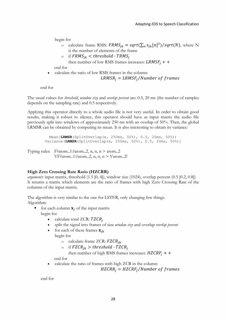
Low Short-Time Energy Ratio (LSTER) arguments: input matrix, threshold (0.15 [0, 1]), window size (1024), overlap percent (0.5 [0.2, 0.8]) It returns a matrix which elements are the ratio of low short-time energy frames of the columns of the input matrix. Algorithm:
for each column of the input matrix begin for
• calculate total energy: ∑ • split the signal into frames of size window size and overlap overlap percent • for each of these frames
begin for o calculate frame energy: ∑ o if ·
then number of low-energy frames increases: end for
• calculate the ratio of low energy frames in the column: ⁄
end for
The usual values for threshold, window size and overlap percent are: 0.15, 20 ms (the number of samples depends on the sampling rate) and 0.5 respectively.
Applying this operator directly to a whole audio file is not very useful. In order to obtain good results, making it robust to silence, this operator should have as input matrix the audio file previously split into windows of approximately 250 ms with an overlap of 50%. Then, the global LSTER can be obtained by computing its mean. It is also interesting to obtain its variance:
Mean(LSTER(SplitOverlap(x, 250ms, 50%), 0.15, 20ms, 50%))
Variance(LSTER(SplitOverlap(x, 250ms, 50%), 0.15, 20ms, 50%)) Typing rules: F?atom_1:?atom_2, n, n, n > atom_2 VF?atom_1:?atom_2, n, n, n > Vatom_2! Low RMS Ratio (LRMSR) arguments: input matrix, threshold (0.5 [0, 1]), window size (1024), overlap percent (0.5 [0.2, 0.8]) It returns a matrix which elements are the ratio of low RMS frames of the columns of the input matrix. The algorithm is very similar to the one for LSTER, only changing few things. Algorithm:
for each column of the input matrix begin for
• calculate total RMS: ∑ ⁄ , where M is the number of elements of the column
• split the signal into frames of size window size and overlap overlap percent • for each of these frames
Adapting EDS to Speech Classification
28
begin for o calculate frame RMS: ∑ ⁄ , where N
is the number of elements of the frame o if ·
then number of low RMS frames increases: end for
• calculate the ratio of low RMS frames in the column: ⁄
end for
The usual values for threshold, window size and overlap percent are: 0.5, 20 ms (the number of samples depends on the sampling rate) and 0.5 respectively.
Applying this operator directly to a whole audio file is not very useful. In order to obtain good results, making it robust to silence, this operator should have as input matrix the audio file previously split into windows of approximately 250 ms with an overlap of 50%. Then, the global LRMSR can be obtained by computing its mean. It is also interesting to obtain its variance:
Mean(LRMSR(SplitOverlap(x, 250ms, 50%), 0.5, 20ms, 50%)) Variance(LRMSR(SplitOverlap(x, 250ms, 50%), 0.5, 20ms, 50%))
Typing rules: F?atom_1:?atom_2, n, n, n > atom_2 VF?atom_1:?atom_2, n, n, n > Vatom_2! High Zero Crossing Rate Ratio (HZCRR) arguments: input matrix, threshold (1.5 [0, 4]), window size (1024), overlap percent (0.5 [0.2, 0.8]) It returns a matrix which elements are the ratio of frames with high Zero Crossing Rate of the columns of the input matrix. The algorithm is very similar to the one for LSTER, only changing few things. Algorithm:
for each column of the input matrix begin for
• calculate total ZCR: • split the signal into frames of size window size and overlap overlap percent • for each of these frames
begin for o calculate frame ZCR: o if ·
then number of high RMS frames increases: end for
• calculate the ratio of frames with high ZCR in the column: ⁄
end for
2.2 New Operators for EDS
29
The usual values for threshold, window size and overlap percent are: 1.5, 20 ms (the number of samples depends on the sampling rate) and 0.5 respectively.
Applying this operator directly to a whole audio file is not very useful. In order to obtain good results, making it robust to silence, this operator should have as input matrix the audio file previously split into windows of approximately 250 ms with an overlap of 50%. Then, the global HZCRR can be obtained by computing its mean. It is also interesting to obtain its variance:
Mean(HZCRR(SplitOverlap(x, 250ms, 50%), 0.5, 20ms, 50%)) Variance(HZCRR(SplitOverlap(x, 250ms, 50%), 0.5, 20ms, 50%))
Typing rules: Ft:a, n, n, n > a VFt:a, n, n, n > Va! Praat Library:
To complete the list of new operators specifically thought for speech classification problems, we used part of Praat, a free computer program for speech analysis, synthesis and manipulation, connecting it to EDS for being the core of the calculus of some new interesting operators. Next, there is a brief explanation of them. The parameters used are always the default ones proposed by Praat. More precise information of the following operators can be found on its online documentation (Boersma and Weenink 2008). Harmonicity (HarmonicitySplitPraat) arguments: input matrix It returns a matrix which elements are the degree (in dB) of acoustic periodicity of the frames of the input matrix, taken as a temporal signal. This short-term acoustic periodicity detection, on the basis of an accurate autocorrelation method, it is also called Harmonics-to-Noise Ratio (HNR). Typing rules: Ft:a > Va! Pitch (PitchSplitPraat) arguments: input matrix It returns a matrix which elements are frequencies (in Hz) of the pitches of the frames of the input matrix, taken as a temporal signal. The algorithm performs an acoustic periodicity detection, optimized for speech, on the basis of an accurate autocorrelation method.
Typing rules: VFt:a > Vf! Formants (FormantSplitPraat) arguments: input matrix It returns a matrix which columns are the frequencies (in Hz) of the formants of the frames of the input matrix, taken as a temporal signal. It performs a short-term spectral analysis, approximating the spectrum of each analysis frame by a number of formants, using an algorithm by Burg.
Adapting EDS to Speech Classification
30
Typing rules: Ft:a > VVf! LPC (LPCCovarianceSplitPraat) It returns a matrix which columns are the Linear Predictive Coding coefficients of the frames of the input matrix, taken as a temporal signal. This algorithm uses the covariance method. Typing rules: Ft:a > VVa!
2.3 Limitations of EDS Despite being a powerful tool, EDS presents, by construction, some limitations which sometimes are not possible to overcome. Here it is a description of those we have found during the work. The first drawback is the fact that the output argument of an operator is limited to a two-dimensional matrix. This dimension is enough for a great number of computations, but it prevents from the implementation of operators that work with three-dimensional matrix, which are quite usual in audio processing. A clear case is described next: EDS allows to work with signal frames (using the operators Split or SplitOverlap), and with filter banks (using FilterBank), having both a two-dimensional output matrix. Nevertheless, the combination of both (Split(FilterBank(x, 16), 1024)) is not possible, since the dimension of the output matrix would be greater than two. The described limitation made impossible the implementation of some possibly interesting operators, derived from the following features: Spectral Balance-Based Cepstral Coefficients (Ren et al. 2004), Subband Spectral Centroids Histograms (Gajic and Paliwal 2001). Derived from the previous limitation, one can deduce that operators can only work with real numbers. This is caused by the fact that if the output matrix of an operator would be complex, it would be necessary an extra dimension to store the imaginary part, leading to some situations of three-dimensional output matrix. The implications of that observation are that an operator like Fft is not able to give its entire complex output, but only its magnitude. Once in the frequency domain, there is no way to return to the temporal domain through an inverse Fourier transform, because the phase information is not kept through the calculations. So, no iFFT operator can be implemented in the system. Another type of limitation is the impossibility of implementing operators that need more than one element of the database to make the calculation. Typical operators of that kind are those which normalize through the entire database. So, operators derived from this idea, like the Augmented Cepstral Normalisation (Acero and Huang 1995), are not implementable. In another direction, a big constraint appears when trying to make genetic searches with vectorial features (i.e. features that give as output a vector, as in the case of MFCCs). There is no way to define the maximum length of a vectorial feature that EDS should explore, and this poses a problem: since longer vectorial features have better fitness than shorter ones, EDS always

2.3 Limitations of EDS
31
rejects by natural selection those vectorial features of short lengths. Thus, it is very difficult, even impossible, to explore and keep good vectorial features of short lengths for next generations, forcing to draw aside the exploration of genetic modifications of classical MFCC-like or LPC-like features, which have typical lengths between 10 and 25. Lastly, the typing rules EDS works with present some limitations that appear in the attempt of simplifying their complexity. This way, there exist some operators which take as input matrix a temporal signal [t:a] that cannot take an array of amplitudes [Va] because the temporal information has been lost. EDS is unable to build, then, a feature like the following: BpFilter(Rms(Split(x))). The output of Split(x) is an array of temporal signals [Vt:a], but in the next step, Rms(Split(x)) gives as output a vector of amplitudes [Va] that cannot be used as input for the filtering operator BpFilter, because BpFilter only accepts temporal signals. This fact makes that theoretically well-formed features, which are semantically correct, are not accepted because of their syntax.

33
Chapter 3
Experimental Work
In order to explore whether EDS and the analytical feature technique can be applied with success to speech classification problems, a series of experiments were carried out. For this purpose, a speech database – described in Section 3.1 – was built, in parallel to the implementation on the system of the new operators defined in Chapter 2. Section 3.2 details the feature patterns that were used in the genetic searches, before a first experiment is presented in Section 3.3. On the basis of the results of the preliminary experiment, an endpoint detector was designed (see Section 3.4) and the experiment was repeated using a modified database. The effect of the new operators are analysed from the experiments detailed in Sections 3.5.2 and 3.5.3, and finally an experiment explores the EDS potential to build analytical vectorial features.
3.1 The Databases The particular problem EDS has to face is defined under the form of a training database. The characteristics of this database will set the characteristics of the problem. To test the performance of the classifier, some test databases are needed. Since no suitable pre-existent databases were found for the purpose of our experiments, new ones were built with the characteristics described in the following sections.
3.1.1 The Training Database
The training set, named TrainDB48, presents the following characteristics:
• Since possible applications of these speech classifiers are toys or low-cost technology used in informal environments, sounds were recorded with a domestic desktop microphone in a desktop computer, in an office environment with background noise.
• The samples were recorded in a Microsoft WAV PCM format at a sampling rate of 48 kHz, and a bit depth of 16 bits, mono.
• The samples consist of isolated words with the presence of silence at the beginning and the end of each utterance.
• There are 12 different words (12 classes): black, blue, brown, cyan, green, grey, orange, pink, red, violet, white and yellow.
Experimental Work
34
• 6 adult subjects: 4 males (AL, GB, GC, PR) and 2 females (MN, SB), with foreign accents: Catalan, Dutch, French and Italian.
• Each subject recorded each word 40 times, obtaining 240 samples per class, and a total of 2880 samples.
3.1.2 The Test Databases Three different databases to test the performance of the classifier were created. The recording method and audio format, as well as the classes, were the same as in the training database. The two first databases are to test the speaker-independent performance of the classifier, since samples are recorded by different subjects from the training database. On the other hand, the third database was build for testing the performance under speaker-dependent environments. First Test Database (TestDB48-1)
• 5 subjects: 3 adult males (FP, MS, V1), 1 adult female (V2) and 1 female child (CP), with foreign accents: Chinese, Dutch, and French.
• Each subject recorded each word 2 times, obtaining 10 samples per class, and a total of 120 samples.
Second Test Database (TestDB48-2)
• 1 adult male (FP) with French accent. • The subject recorded each word 30 times, obtaining 30 samples per class, and a total of
360 samples.
Third Test Database (TestDB48-3)
• 5 adult subjects: 3 males (AL, GB, PR), and 2 females (MN, SB), with foreign accents: Dutch, French and Italian.
• Each subject recorded each word 2 times, obtaining 10 samples per class, and a total of 120 samples.
3.2 Pattern Sets To make the genetic search of the features more efficient and exhaustive, it was divided in three parts, using three different sets of patterns. The idea was to launch three genetic searches in parallel, focusing each one on a specific type of feature.
EDS tries always to move from one type of signal to another in the simplest and shortest way. Thus, a long list of highly specified patterns was set in order to use the greatest number of operator combinations. In that sense, for example, the pattern expression [...!_f (!_t:a ...)] would

3.2 Pattern Sets
35
not be enough to make the FormantSplitPraat operator to appear. A more specific pattern expression is necessary: [...!_f (!_VVf (!_t:a ...)].
First, a set of 25 patterns that allowed EDS to explore those features that do not split either in time or in frequency:
!_a (x) !_a (!_t:a (x)) !_a (!_Va (x)) !_a (!_Va (!_t:a (x))) !_t (x) !_t (!_t:a (x)) !_t (!_Vt (x)) !_t (!_Vt (!_t:a (x))) !_f (x) !_f (!_f:a (x)) !_f (!_Vf (x)) !_f (!_Vf (!_f:a (x))) !_f (!_t:a (x)) !_a (!_f:a (!_t:a (x))) !_f (!_f:a (!_t:a (x))) !_a (!_Va (!_f:a (!_t:a (x)))) !_f (!_Vf (!_f:a (!_t:a (x)))) !_a (!_t:a (!_f:a (x))) !_t (!_t:a (!_f:a (x))) !_a (!_Va (!_t:a (!_f:a (x)))) !_t (!_t:a (!_f:a (x))) !_t (!_Vt (!_t:a (!_f:a (x)))) !_f (!_VVf (!_t:a(x))) !_f (!_Vf (!_t:a (x))) !_a (!_VVa (!_t:a (x))) Second, a set of 15 patterns that allowed EDS to explore those features that split in time: !_a (Hamming (SplitOverlap (!_t:a (x), 1024.0, 0.5))) !_t (Hamming (SplitOverlap (!_t:a (x), 1024.0, 0.5))) !_f (Hamming (SplitOverlap (!_t:a (x), 1024.0, 0.5))) !_a (!_Vt:a (Hamming (SplitOverlap (!_t:a (x), 1024.0, 0.5)))) !_t (!_Vt:a (Hamming (SplitOverlap (!_t:a (x), 1024.0, 0.5)))) !_f (!_Vt:a (Hamming (SplitOverlap (!_t:a (x), 1024.0, 0.5)))) !_a (!_VVa (Hamming (SplitOverlap (!_t:a (x), 1024.0, 0.5)))) !_a (!_Vf:a (Hamming (SplitOverlap (!_t:a (x), 1024.0, 0.5)))) !_f (!_Vf:a (Hamming (SplitOverlap (!_t:a (x), 1024.0, 0.5)))) !_a (!_VVa (!_Vf:a (Hamming (SplitOverlap (!_t:a (x), 1024.0,
0.5))))) !_f (!_VVf (Hamming (SplitOverlap (!_t:a (x), 1024.0, 0.5)))) !_a (!_t:a (Hamming (SplitOverlap (!_t:a (x), 1024.0, 0.5)))) !_t (!_t:a (Hamming (SplitOverlap (!_t:a (x), 1024.0, 0.5)))) !_f (!_t:a (Hamming (SplitOverlap (!_t:a (x), 1024.0, 0.5)))) !_a (!_Va (!_t:a (Hamming (SplitOverlap (!_t:a (x), 1024.0, 0.5))))) Note that before the temporal split, there is a degree of freedom left to EDS to use an
operator that preprocesses the samples. The length and overlap of the window frames are specified by the arguments of SplitOverlap (in that case 1024, to get frames of about 20 ms at 48 kHz, and 0.5, for an overlap of 50%). After the temporal split, a Hamming windowing is applied to each frame.
Experimental Work
36
Third, a set of 12 patterns that allowed EDS to explore those features that split mainly in
the frequency domain: !_a (!_Vf:a (!_f:a (x))) !_f (!_Vf:a (!_f:a (x))) !_t (!_Vf:a (!_f:a (x))) !_a (!_VVa (!_Vf:a (!_f:a (x)))) !_f (!_VVf (!_Vf:a (!_f:a (x)))) !_t (!_Vf:a (!_f:a (x))) !_a (!_Vf:a (!_f:a (!_t:a (x))))) !_f (!_Vf:a (!_f:a (!_t:a (x))))) !_t (!_Vf:a (!_f:a (!_t:a (x))))) !_a (!_t:a (!_Vf:a (!_f:a (!_t:a (x)))))) !_a (!_VVa (!_Vf:a (!_f:a (!_t:a (x))))) !_f (!_VVf (!_Vf:a (!_f:a (!_t:a (x)))))
3.3 The First Experiment
Using the training database, three genetic searches (one for each set of patterns) were launched with only the old operators enabled. After putting together the three sets of features explored by EDS, corresponding to the three independent searches, the feature selection tool of EDS was used to select the 10 best features:
Percentile (HMedian (Mfcc0 (Hamming (SplitOverlap (Normalize (x), 1024.0, 0.5)), 10.0)), 50.0)
Log10 (Kurtosis (LtasPCPraat (x))) Power (Iqr (Mfcc0 (LpFilter (x, 100.0), 12.0)), 0.6) Square (SpectralSpread (Triangle (x))) Power (Abs (Iqr (Mfcc0 (Arcsin (x), 6.0))), 1.6) Min (HSkewness (BarkBands (Fft (Hamming (SplitOverlap (Bartlett (x),
1024.0, 0.5))), 5.0))) Iqr (MelBands (Normalize (x), 10.0)) Percentile (Mfcc (x, 10.0), 86.0) Square (MaxPos (LtasPraat (BpFilter (x, 857.0, 411.0)))) Iqr (Nth (MelBands (SplitOverlap (Fft (Normalize (x)), 32.0, 0.5),
5.0), 1.0)) A classifier was built with Weka, using SMO (Sequential Minimal Optimization), a fast
method to speed up the training of the Support Vector Machines (SVM). The results of the correctly classified instances of the three test databases are as follows (detailed results can be found in the Appendix II):
TestDB48-1: 30.83 % TestDB48-2: 29.44 % TestDB48-3: 69.17 % Note that the results in the third case are much better than in the other two. This is
because the third test is in a speaker-dependent context. That means, then, that the features found in this experiment by EDS work much better in a speaker-dependent context than in a speaker-independent one.
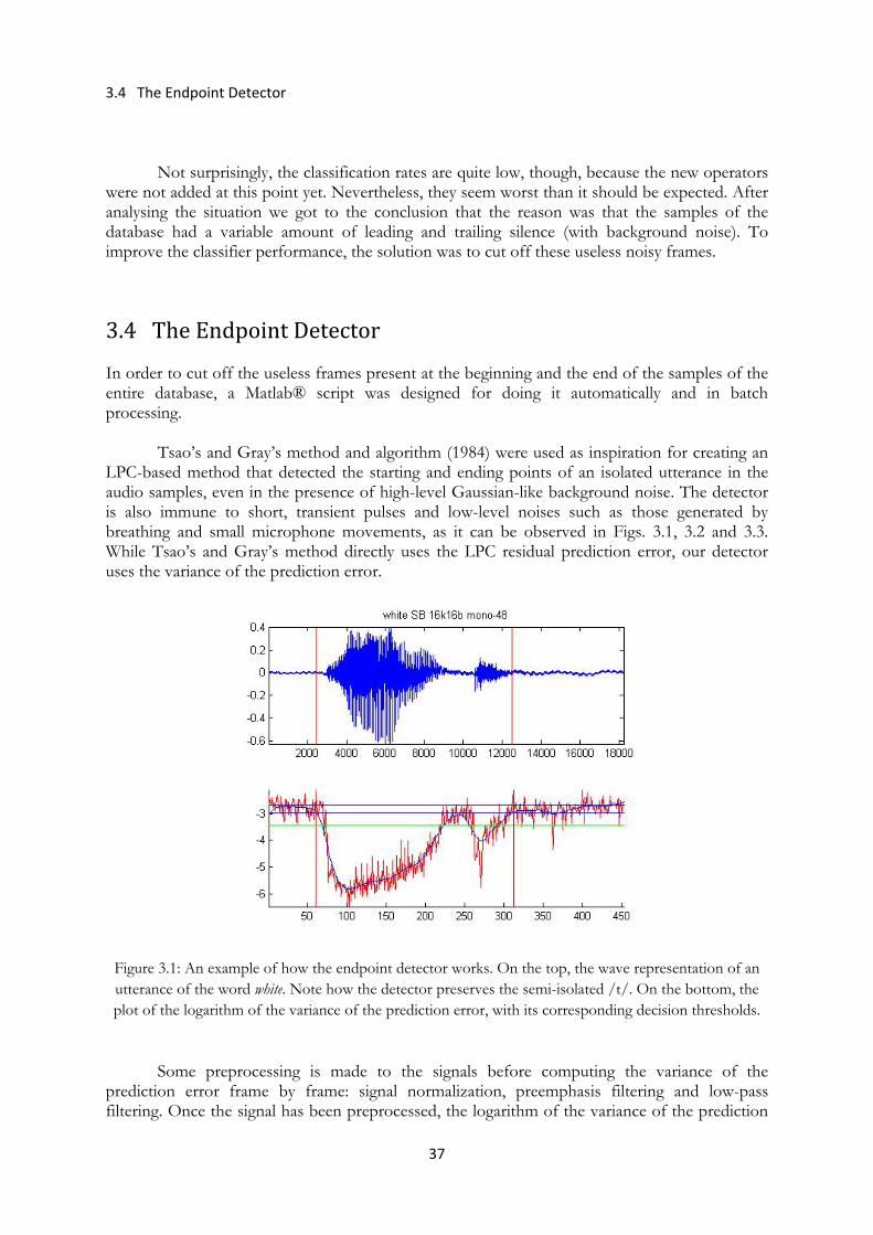
3.4 The Endpoint Detector
37
Not surprisingly, the classification rates are quite low, though, because the new operators
were not added at this point yet. Nevertheless, they seem worst than it should be expected. After analysing the situation we got to the conclusion that the reason was that the samples of the database had a variable amount of leading and trailing silence (with background noise). To improve the classifier performance, the solution was to cut off these useless noisy frames.
3.4 The Endpoint Detector In order to cut off the useless frames present at the beginning and the end of the samples of the entire database, a Matlab® script was designed for doing it automatically and in batch processing.
Tsao’s and Gray’s method and algorithm (1984) were used as inspiration for creating an LPC-based method that detected the starting and ending points of an isolated utterance in the audio samples, even in the presence of high-level Gaussian-like background noise. The detector is also immune to short, transient pulses and low-level noises such as those generated by breathing and small microphone movements, as it can be observed in Figs. 3.1, 3.2 and 3.3. While Tsao’s and Gray’s method directly uses the LPC residual prediction error, our detector uses the variance of the prediction error.
Figure 3.1: An example of how the endpoint detector works. On the top, the wave representation of an utterance of the word white. Note how the detector preserves the semi-isolated /t/. On the bottom, the plot of the logarithm of the variance of the prediction error, with its corresponding decision thresholds.
Some preprocessing is made to the signals before computing the variance of the prediction error frame by frame: signal normalization, preemphasis filtering and low-pass filtering. Once the signal has been preprocessed, the logarithm of the variance of the prediction
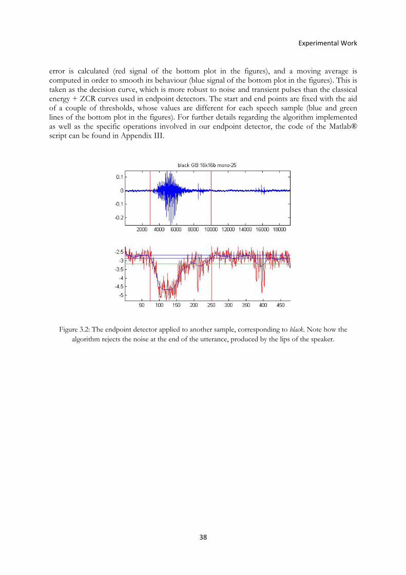
Experimental Work
38
error is calculated (red signal of the bottom plot in the figures), and a moving average is computed in order to smooth its behaviour (blue signal of the bottom plot in the figures). This is taken as the decision curve, which is more robust to noise and transient pulses than the classical energy + ZCR curves used in endpoint detectors. The start and end points are fixed with the aid of a couple of thresholds, whose values are different for each speech sample (blue and green lines of the bottom plot in the figures). For further details regarding the algorithm implemented as well as the specific operations involved in our endpoint detector, the code of the Matlab® script can be found in Appendix III.
Figure 3.2: The endpoint detector applied to another sample, corresponding to black. Note how the algorithm rejects the noise at the end of the utterance, produced by the lips of the speaker.
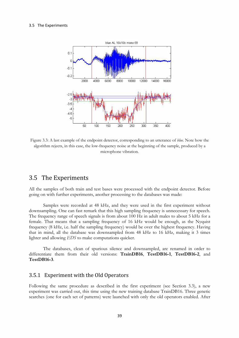
3.5 The Experiments
39
Figure 3.3: A last example of the endpoint detector, corresponding to an utterance of blue. Note how the algorithm rejects, in this case, the low-frequency noise at the beginning of the sample, produced by a
microphone vibration.
3.5 The Experiments All the samples of both train and test bases were processed with the endpoint detector. Before going on with further experiments, another processing to the databases was made: Samples were recorded at 48 kHz, and they were used in the first experiment without downsampling. One can fast remark that this high sampling frequency is unnecessary for speech. The frequency range of speech signals is from about 100 Hz in adult males to about 5 kHz for a female. That means that a sampling frequency of 16 kHz would be enough, as the Nyquist frequency (8 kHz, i.e. half the sampling frequency) would be over the highest frequency. Having that in mind, all the database was downsampled from 48 kHz to 16 kHz, making it 3 times lighter and allowing EDS to make computations quicker. The databases, clean of spurious silence and downsampled, are renamed in order to differentiate them from their old versions: TrainDB16, TestDB16-1, TestDB16-2, and TestDB16-3.
3.5.1 Experiment with the Old Operators Following the same procedure as described in the first experiment (see Section 3.3), a new experiment was carried out, this time using the new training database TrainDB16. Three genetic searches (one for each set of patterns) were launched with only the old operators enabled. After
Experimental Work
40
putting together the three sets of features explored by EDS, corresponding to the three independent searches, the feature selection tool of EDS was used to select the 10 best features:
Skewness (Integration (PeakPos (Integration (BpFilter (x, 2205.0,
752.0))))) Skewness (Abs (PeakPos (LpFilter (Hann (Arcsin (x)), 441.0)))) Power (Abs (Centroid (Variance (BarkBands (Fft (Arcsin (SplitOverlap
(Power (Hamming (x), 3.0), 320.0, 0.8))), 5.0)))), -1.0) Skewness (PeakPos (Hanning(x))) Centroid (SpectralSkewness (Hamming (SplitOverlap (Normalize (x),
4410.0, 0.3)))) Power (Abs (Centroid (Iqr (BarkBands (Fft (Arcsin (SplitOverlap
(Power (HpFilter (x, 100.0), 3.0), 320.0, 0.8))), 5.0)))), -1.0)
Rms (Zcr (SplitOverlap (Power (Hamming(x), 3.0), 320.0, 0.8))) Power (Centroid (Peaks (Integration (BpFilter (Derivation (Hamming
(x)), 766.0, 98.0)))), -0.7) Power (Abs (Centroid (Peaks (Abs (BpFilter (x, 766.0, 98.0))))), -
2.1) Power (Abs (Centroid (Peaks (Blackman (Normalize (x))))), -0.4)
A classifier was built with Weka, using SMO. The results of the correctly classified
instances of the three test databases are as follows (detailed results can be found in the Appendix IV):
TestDB16-1: 49.17 % TestDB16-2: 47.22 % TestDB16-3: 79.17 % Note that, again, the results in the third case are much better than the other two. This is
because the third test is in a speaker-dependent context. That means, then, that the features found in this experiment by EDS work much better in a speaker-dependent context than in a speaker-independent one.
As expected, the results are sensibly better than before cleaning the database with the
endpoint detector: the performance has improved 18.34, 17.78 and 10 points respectively.
3.5.2 Experiment with the Old and New Operators In order to test the suitability of the new operators (described in Section 2.2) for speech classification problems, the next experiment lay in repeating the previous one but adding the new operators to the system. To succeed, the results of this experiment should be sensibly better. Using the training database TrainDB16, three genetic searches (one for each set of patterns) were launched with all operators enabled this time. After putting together the three sets of features explored by EDS, corresponding to the three independent searches, the feature selection tool of EDS was used to select the 10 best features:
Skewness (PeakPos (BpFilter (VmeanNormalization (VmeanNormalization
(x)), 2205.0, 706.0))) Power (Zcr (HFPreemphasis (BpFilter (Power (HFPreemphasis
(Multiplication (x, 2.11), 5.0), 3.0), 2205.0, 706.0), 0.9709857365633688)), -0.3)

3.5 The Experiments
41
Skewness (PeakPos (BpFilter (HFPreemphasis (Derivation (Hamming (HFPreemphasis (x, 5.0))), 5.0), 2205.0, 706.0)))
Skewness (PeakPos (Integration (BpFilter (LPCResidualError (HFPreemphasis (x, 0.9945909981191632), 5.0), 676.0, 89.0))))
Skewness (PeakPos (Integration (Bartlett(x)))) Skewness (PeakPos (Abs (Integration (BpFilter (LPCResidualError
(Hamming (x), 5.0), 676.0, 89.0))))) Power (SpectralCentroid (HFPreemphasis (BpFilter (HFPreemphasis
(HFPreemphasis (x, 5.0), 5.0), 1764.0, 706.0), 0.980802238935936)), -0.3)
Skewness (PeakPos (Arcsin (Multiplication (x, 5.0)))) Power (Zcr (HFPreemphasis (BpFilter (Power (HFPreemphasis
(HFPreemphasis (x, 0.9305338823473828), 5.0), 3.0), 2205.0, 706.0), 0.930205069958596)), -0.3)
Skewness (PeakPos (Integration (BpFilter (VregressionCoeffs (Triangle (Integration (VregressionCoeffs (x, 3.0))), 5.0), 676.0, 89.0))))
A classifier was built with Weka, using SMO. The results of the correctly classified
instances of the three test databases are as follows (detailed results can be found in the Appendix V):
TestDB16-1: 56.67 % TestDB16-2: 62.22 % TestDB16-3: 80.00 % The speaker-dependent case (TestDB16-3) yields, as expected, the best results. Comparing these results with the ones of the previous experiment, we can see that there
is an improvement in all three cases: 7.5 points in the first, 15 in the second, and 0.84 in the last one. The improvement in the speaker-independent situations is notable, while in the speaker-dependent case, results are roughly the same. That leads to the idea that the new operators help to classify speaker-independent speech, while it seems difficult to improve the speaker-dependent speech recognition performance by adding more operators to the system.
Something that has to be observed is that 8 out of 10 features have at least one new
operator. On the other hand, only 4 out of 23 new operators were used: HFPreemphasis (x11), LPCResidualError (x2), VMeanNormalization (x2), VRegressionCoeffs (x2).
3.5.3 Experiment with the Old and New Operators and up to 35 Features All the experiments carried out till that point were done taking a relatively small number of features, taking into account the complexity of the problem.
To test the behaviour of our approach when increasing the number of features, a new experiment was performed. Starting from exactly the same situation than the previous experiment, the best 35 analytical features were selected using the feature selection tool of EDS:
Skewness (PeakPos (BpFilter (VmeanNormalization (VmeanNormalization
(x)), 2205.0, 706.0)))

Experimental Work
42
Power (Zcr (HFPreemphasis (BpFilter (Power (HFPreemphasis (Multiplication (x, 2.11), 5.0), 3.0), 2205.0, 706.0), 0.9709857365633688)), -0.3)
Skewness (PeakPos (BpFilter (HFPreemphasis (Derivation (Hamming (HFPreemphasis (x, 5.0))), 5.0), 2205.0, 706.0)))
Skewness (PeakPos (Integration (BpFilter (LPCResidualError (HFPreemphasis (x, 0.9945909981191632), 5.0), 676.0, 89.0))))
Skewness (PeakPos (Integration (Bartlett(x)))) Skewness (PeakPos (Abs (Integration (BpFilter (LPCResidualError
(Hamming (x), 5.0), 676.0, 89.0))))) Power (SpectralCentroid (HFPreemphasis (BpFilter (HFPreemphasis
(HFPreemphasis (x, 5.0), 5.0), 1764.0, 706.0), 0.980802238935936)), -0.3)
Skewness (PeakPos (Arcsin (Multiplication (x, 5.0)))) Power (Zcr (HFPreemphasis (BpFilter (Power (HFPreemphasis
(HFPreemphasis (x, 0.9305338823473828), 5.0), 3.0), 2205.0, 706.0), 0.930205069958596)), -0.3)
Skewness (PeakPos (Integration (BpFilter (VregressionCoeffs (Triangle (Integration (VregressionCoeffs (x, 3.0))), 5.0), 676.0, 89.0))))
Log10 (Norm (Zcr (Hamming (SplitOverlap (HFPreemphasis (VmeanNormalization (x), -1.0), 320.0, 0.5)))))
Sqrt (Centroid (PeakPos (Integration (BpFilter (VregressionCoeffs (Triangle (VmeanNormalization (x)), 5.0), 676.0, 89.0)))))
Skewness (PeakPos (Square (BpFilter (VregressionCoeffs (Bartlett (x), 5.0), 676.0, 89.0))))
Skewness (PeakPos (BpFilter (VregressionCoeffs (Hamming (Abs (x)), 3.0), 2205.0, 706.0)))
Skewness (PeakPos (Abs (VmeanNormalization (VregressionCoeffs (BpFilter (Integration (VregressionCoeffs (x, 2.0)), 2205.0, 706.0), 5.0)))))
Power (Abs (SpectralSpread (Abs (BpFilter (LPCResidualError (HFPreemphasis (Triangle (x), 0.9692254851728542), 5.0), 676.0, 89.0)))), 4.6)
Sqrt (Centroid (PeakPos (Integration (BpFilter (VregressionCoeffs (Multiplication (Hann (x), 5.9), 5.0), 7938.0, 89.0)))))
Power (Skewness (PeakPos (Abs (VmeanNormalization (VregressionCoeffs (Derivation (Hamming (x)), 5.0))))), 3.0)
Power (SpectralCentroid (Fft (Fft (x))), 3.0) Abs (Skewness (PeakPos (Integration (BpFilter (LPCResidualError
(HFPreemphasis (Triangle (Normalize (x)), 0.9945909981191632), 5.0), 676.0_89.0)))))
Log10 (SpectralFlatness (x)) Abs (Skewness (PeakPos (BpFilter (VmeanNormalization (HFPreemphasis
(HFPreemphasis (Triangle (x), 5.0), 5.0)), 2205.0, 706.0)))) Power (Zcr (HFPreemphasis (BpFilter (VregressionCoeffs (x, 3.0),
2205.0, 1764.0), 0.9982319335180304)), -3.9) Abs (Skewness (PeakPos (BpFilter (Blackman (Hanning (x)), 2205.0,
706.0)))) Power (Zcr (Peaks (Derivation (x))), 1.8) MaxPos (Peaks (Hamming (x))) Bandwidth (BpFilter (x, 234.0, 648.0), 50.0) Power (Kurtosis (PeakPos (Derivation (Fft (Blackman (Derivation
(x)))))), -0.4) Sqrt (SpectralSpread (BpFilter (x, 981.0, 556.0))) Skewness (PeakPos (BpFilter (Arcsin (Derivation (x)), 2205.0,
706.0))) Skewness (PeakPos (Power (x, 3.0))) Skewness (PeakPos (Integration (Bartlett (x))))
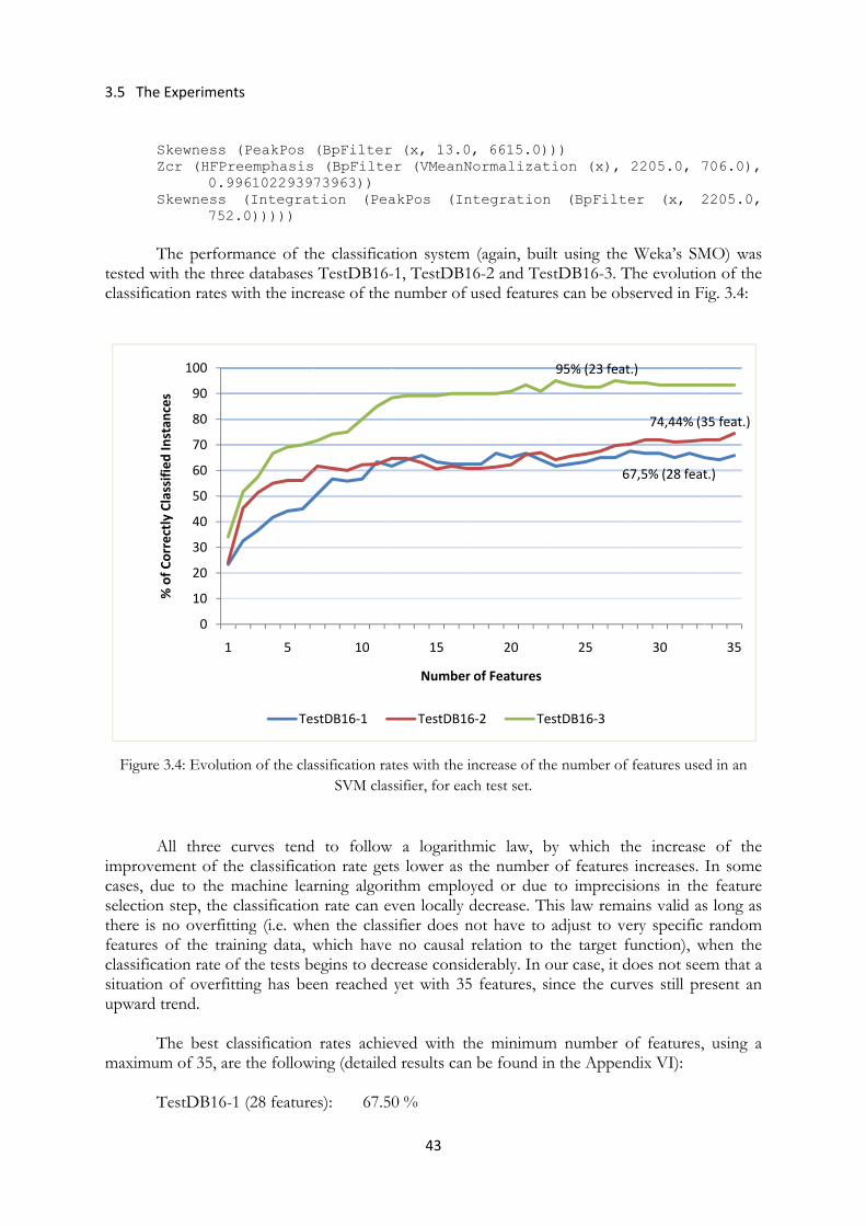
3.5 The
T
tested wclassific
Figure
Aimprovecases, dselectionthere is featuresclassificsituationupward
Tmaximu
T
e Experiment
Skewness Zcr (HFPr
0.9Skewness
752
The performwith the threcation rates w
e 3.4: Evoluti
All three cement of thdue to the mn step, the cno overfitt
s of the traication rate on of overfittrend.
The best clum of 35, are
TestDB16-1
0
10
20
30
40
50
60
70
80
90
100
1
% of C
orrectly Classified
Instan
ces
ts
(PeakPos eemphasis961022939(Integrat.0)))))
mance of thee databaseswith the incr
ion of the cla
curves tendhe classificatmachine leaclassificationting (i.e. whining data, wf the tests btting has be
lassification e the follow
1 (28 feature
5
Te
(BpFilter (BpFilte73963)) tion (Pea
he classificat TestDB16-rease of the
assification raSVM clas
d to followtion rate getrning algorin rate can ev
hen the classwhich haveegins to decen reached
rates achiewing (detailed
es): 67.5
10
stDB16‐1
43
r (x, 13.0er (VMeanN
akPos (In
tion system-1, TestDB1number of
tes with the issifier, for eac
w a logarithts lower as tithm emploven locally dsifier does n no causal
crease considyet with 35
eved with thd results can
0 %
15
Number
TestDB16
, 6615.0)Normalizat
ntegration
(again, bui16-2 and Tesused feature
increase of thch test set.
hmic law, bthe numberyed or due decrease. Th
not have to relation to derably. In o5 features, s
he minimumn be found in
20
r of Features
6‐2 Te
)) tion (x),
n (BpFilt
ilt using thestDB16-3. Tes can be ob
he number of
by which thr of features
to imprecihis law remaadjust to vthe target f
our case, it dince the cur
m number on the Appen
6
95% (23 feat
25
estDB16‐3
2205.0, 7
ter (x, 2
e Weka’s SMThe evolutiobserved in Fi
f features use
he increases increases. sions in theains valid asery specific function), wdoes not seerves still pr
of features, ndix VI):
67,5% (28 feat
74,44% (3
t.)
30
706.0),
2205.0,
MO) was on of the ig. 3.4:
d in an
e of the In some e feature s long as random
when the em that a resent an
using a
t.)
35 feat.)
35
Experimental Work
44
TestDB16-2 (35 features): 74.44 % TestDB16-3 (23 features): 95.00 %
As it can be observed, the improvement in the results of all three cases with the use 35
features is very interesting. The speaker-dependent case presents almost a perfect performance. In this experiment, like in the previous one, there is a numerous presence of new
operators: 20 out of 35 features have at least one new operator. Nevertheless, only 5 out of 23 new operators were used: HFPreemphasis (x18), VRegressionCoeffs (x10), VMeanNormalization (x8), LPCResidualError (x4) and Norm (x1), the same ones as in the last experiment plus Norm. This, among other reasons, can appear due to the way EDS explores the feature space and also the feature selection technique used by the system.
3.5.4 Experiment with an MFCC‐like Feature The last experiment was a little bit different from the others. The idea was to let EDS find a feature derived from the MFCC. This vectorial MFCC-like feature should be of length 10 in order to compare the results with the ones of the other experiments described in Sections 3.5.1 and 3.5.2.
In order to let EDS explore the MFCC-like feature space, a special set of patterns was created:
Mfcc0 (!_t:a (x), 10) Mfcc0 (!_t:a (!_Vt:a (!_t:a (x))), 10.0) Mfcc0 (!_t:a (Hamming (SplitOverlap (!_t:a (x), 320.0, 0.5)))), 10) Mfcc0 (!_t:a (!_Vt:a (Hamming (SplitOverlap (!_t:a (x), 320.0,
0.5)))), 10) The particular architecture of EDS does not allow doing a detailed genetic search of
vectorial features, as explained in the section Limitations of EDS (2.3). The patterns have to limit EDS to build analytical features that have Mfcc0 as last operator, because adding a vectorial “wild card” (Va, Vt or Vf) after Mfcc0 would give EDS freedom to explore vectorial features without any size limit. Despite these restrictions, the proposed pattern set allows EDS to explore a subspace of the vectorial features we are interested in.
Using the training database TrainDB16, a genetic search was launched with all operators
enabled. The best feature of size 10 that EDS found, with the previous pattern set, was:
Mfcc0 (Hmean (Arcsin (Blackman (SplitOverlap (x, 8820.0, 0.5)))), 10.0)
A classifier was built with Weka, using SMO. The results of the correctly classified
instances of the three test databases are as follows (detailed results can be found in the Appendix VII):
TestDB16-1: 48.33 % TestDB16-2: 50.83 % TestDB16-3: 82.50 %

3.5 The Experiments
45
These results reveal that this vectorial MFCC-like feature is well adapted to the speaker-dependent case, better than no other in the previous experiments with 10 features (in Section 3.5.2 the percentage of correctly classified was 80.00%). On the other hand, the results for TestDB16-1 and TestDB16-2 do not beat the ones achieved in the experiment of Section 3.5.2. This leads to the idea that this MFCC-like feature keeps the information of the speaker and performs worst in a speaker-independent context.

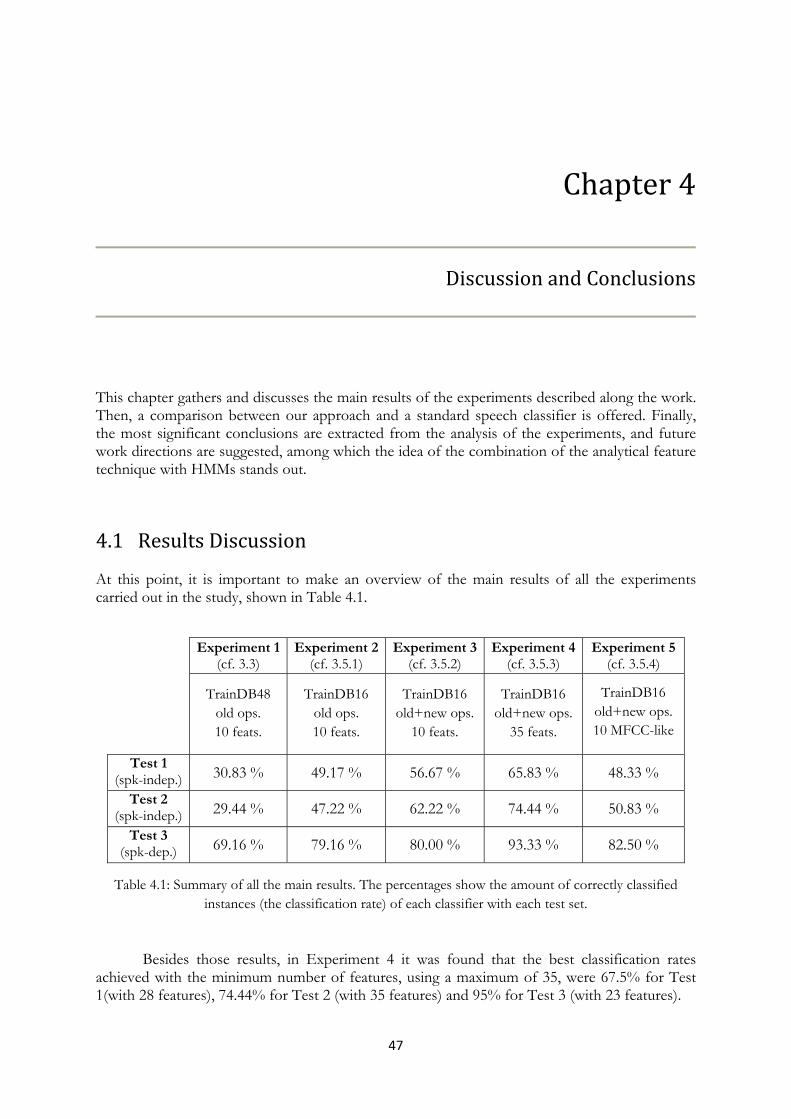
47
Chapter 4
Discussion and Conclusions
This chapter gathers and discusses the main results of the experiments described along the work. Then, a comparison between our approach and a standard speech classifier is offered. Finally, the most significant conclusions are extracted from the analysis of the experiments, and future work directions are suggested, among which the idea of the combination of the analytical feature technique with HMMs stands out.
4.1 Results Discussion At this point, it is important to make an overview of the main results of all the experiments carried out in the study, shown in Table 4.1.
Experiment 1 (cf. 3.3)
Experiment 2(cf. 3.5.1)
Experiment 3(cf. 3.5.2)
Experiment 4 (cf. 3.5.3)
Experiment 5 (cf. 3.5.4)
TrainDB48
old ops. 10 feats.
TrainDB16 old ops. 10 feats.
TrainDB16 old+new ops.
10 feats.
TrainDB16 old+new ops.
35 feats.
TrainDB16 old+new ops. 10 MFCC-like
Test 1 (spk-indep.) 30.83 % 49.17 % 56.67 % 65.83 % 48.33 %
Test 2 (spk-indep.) 29.44 % 47.22 % 62.22 % 74.44 % 50.83 %
Test 3 (spk-dep.) 69.16 % 79.16 % 80.00 % 93.33 % 82.50 %
Table 4.1: Summary of all the main results. The percentages show the amount of correctly classified instances (the classification rate) of each classifier with each test set.
Besides those results, in Experiment 4 it was found that the best classification rates
achieved with the minimum number of features, using a maximum of 35, were 67.5% for Test 1(with 28 features), 74.44% for Test 2 (with 35 features) and 95% for Test 3 (with 23 features).

Discussion and Conclusions
48
The results of each experiment have been discussed in its corresponding section. Let’s sum up here the most relevant ideas:
• The great improvement between Experiment 1 and 2 is thanks to the cleaning made by the endpoint detector processing. Non-speech frames at the beginning and the end of the samples should be always removed. We understand that this preprocessing is something crucial in order to improve the classifier performance.
• The new operators appear to be useful for improving the performance in the speaker-independent cases, although not in the speaker-dependent one. On the other hand, despite the important presence of new operators in the best features built by EDS, only few of them were used. This does not necessarily mean that the other operators are not suitable for speech classification. We can ascribe this behaviour, to a certain extent, to a bias of the genetic search algorithm.
• When the number of features increases, the results improve following a logarithmic law. They improve substantially when adding more features to the only 10 used in Experiment 3. It has been shown that with 23 features a correct classification of the 95% is achieved in the speaker-dependent case, compared to the 80% that yielded the classifier built with 10 features.
• The best vectorial MFCC-like feature of length 10 performs worst than the 10 features built by EDS in the Experiment 3 for the speaker-independent cases, while its performance in the speaker-dependent case is slightly better.
• Observing the F-measures of the different classes, we can note that there are words that tend to be easier to classify through all the experiments (e.g. pink), while other are harder (e.g. red). This confirms the great variability existing in the pronunciation of certain words, and how hard it is to find features that help to classify them.
• As a general remark, as it was expected, the results in the speaker-dependent situation are always better than in the speaker-independent cases, since these ones present a more difficult challenge.
4.2 Comparison with a Standard Speech Classifier It is interesting to compare the results of our approach with those of a standard reference, using the same speech database as in our experiments. This standard ASR system has been built with a widely known and discussed software toolkit developed by the Cambridge University Engineering Department (CUED), the Hidden Markov Model Toolkit (HTK), used for speech recognition research to create state-of-the-art ASR systems (Young et al. 2008).
HTK provides sophisticated tools for building and manipulating hidden Markov models, with facilities for speech analysis, testing and results analysis. Although the tool is often
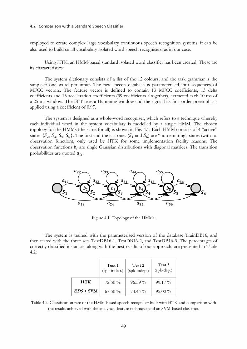
4.2 Comparison with a Standard Speech Classifier
49
employed to create complex large vocabulary continuous speech recognition systems, it can be also used to build small vocabulary isolated word speech recognisers, as in our case.
Using HTK, an HMM-based standard isolated word classifier has been created. These are
its characteristics: The system dictionary consists of a list of the 12 colours, and the task grammar is the
simplest: one word per input. The raw speech database is parameterised into sequences of MFCC vectors. The feature vector is defined to contain 13 MFCC coefficients, 13 delta coefficients and 13 acceleration coefficients (39 coefficients altogether), extracted each 10 ms of a 25 ms window. The FFT uses a Hamming window and the signal has first order preemphasis applied using a coefficient of 0.97.
The system is designed as a whole-word recogniser, which refers to a technique whereby
each individual word in the system vocabulary is modelled by a single HMM. The chosen topology for the HMMs (the same for all) is shown in Fig. 4.1. Each HMM consists of 4 “active” states { , , , }. The first and the last ones ( and ) are “non emitting” states (with no observation function), only used by HTK for some implementation facility reasons. The observation functions are single Gaussian distributions with diagonal matrices. The transition probabilities are quoted .
Figure 4.1: Topology of the HMMs.
The system is trained with the parameterised version of the database TrainDB16, and then tested with the three sets TestDB16-1, TestDB16-2, and TestDB16-3. The percentages of correctly classified instances, along with the best results of our approach, are presented in Table 4.2:
Test 1
(spk-indep.)Test 2
(spk-indep.)
Test 3 (spk-dep.)
HTK 72.50 % 96.39 % 99.17 %
EDS + SVM 67.50 % 74.44 % 95.00 %
Table 4.2: Classification rate of the HMM-based speech recogniser built with HTK and comparison with the results achieved with the analytical feature technique and an SVM-based classifier.
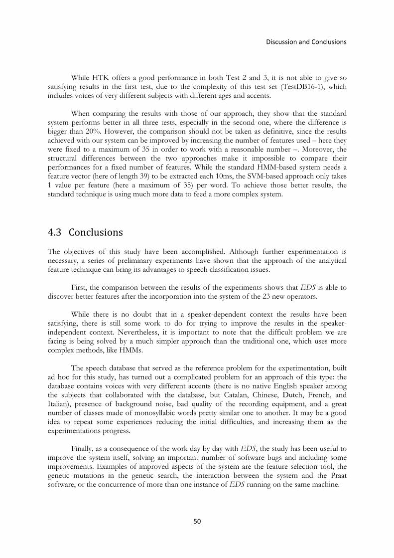
Discussion and Conclusions
50
While HTK offers a good performance in both Test 2 and 3, it is not able to give so satisfying results in the first test, due to the complexity of this test set (TestDB16-1), which includes voices of very different subjects with different ages and accents.
When comparing the results with those of our approach, they show that the standard system performs better in all three tests, especially in the second one, where the difference is bigger than 20%. However, the comparison should not be taken as definitive, since the results achieved with our system can be improved by increasing the number of features used – here they were fixed to a maximum of 35 in order to work with a reasonable number –. Moreover, the structural differences between the two approaches make it impossible to compare their performances for a fixed number of features. While the standard HMM-based system needs a feature vector (here of length 39) to be extracted each 10ms, the SVM-based approach only takes 1 value per feature (here a maximum of 35) per word. To achieve those better results, the standard technique is using much more data to feed a more complex system.
4.3 Conclusions The objectives of this study have been accomplished. Although further experimentation is necessary, a series of preliminary experiments have shown that the approach of the analytical feature technique can bring its advantages to speech classification issues. First, the comparison between the results of the experiments shows that EDS is able to discover better features after the incorporation into the system of the 23 new operators. While there is no doubt that in a speaker-dependent context the results have been satisfying, there is still some work to do for trying to improve the results in the speaker-independent context. Nevertheless, it is important to note that the difficult problem we are facing is being solved by a much simpler approach than the traditional one, which uses more complex methods, like HMMs. The speech database that served as the reference problem for the experimentation, built ad hoc for this study, has turned out a complicated problem for an approach of this type: the database contains voices with very different accents (there is no native English speaker among the subjects that collaborated with the database, but Catalan, Chinese, Dutch, French, and Italian), presence of background noise, bad quality of the recording equipment, and a great number of classes made of monosyllabic words pretty similar one to another. It may be a good idea to repeat some experiences reducing the initial difficulties, and increasing them as the experimentations progress.
Finally, as a consequence of the work day by day with EDS, the study has been useful to improve the system itself, solving an important number of software bugs and including some improvements. Examples of improved aspects of the system are the feature selection tool, the genetic mutations in the genetic search, the interaction between the system and the Praat software, or the concurrence of more than one instance of EDS running on the same machine.
4.4 Future Work
51
4.4 Future Work This work makes an initial assertive step towards the study of the potential of EDS in the domain of speech recognition. During the execution of the thesis, some interesting ideas have been set out in order to continue with the research.
The experiments carried out in the thesis have been only a preliminary approach to the problem. More experimentation is needed in order to come to solid conclusions. It is necessary to work with other databases and assess the performance of the system in other situations. During this study, another database was being created, of 20 classes (this time with the names of 20 different musical genres).
In order to improve the performance of the analytical feature technique, other specific
operators could be implemented, derived from well-known features thought for speech: Daubechies Wavelet Coefficient Histogram (DWCH) (Li and Ogihara 2006), Rasta-PLP (Hermansky et al. 1991), 4 Hz Modulation (Sheirer and Slaney 1997), which have not been finally implemented because of time constraints and complexity.
Lastly, there is an interesting idea of incorporating the EDS analytical features to an
HMM-based recogniser through HTK, which could be the topic of a next study on the adaptation of EDS to speech recognition. In Section 4.2, a comparison was made between a standard speech recogniser (based on HMMs and MFCC) and the system that we designed (an SVM classifier that takes as features the analytical features built by EDS). The results showed that even a state-of-the-art system has problems with certain test sets. On the other hand, one of the biggest drawbacks of the SVM-based technique is that it lacks time alignment, which is well solved by the standard system. The idea is to combine the two approaches, replacing the generic MFCC features of the HMM-based system with analytical features adapted to the problem. To do so, EDS has to be modified so that it produces features for an HMM-based recogniser, which can be achieved by evaluating the analytical features in the genetic search step with a classifier created with HTK. These modifications are technically feasible, as our first attempts indicate, but they are not straightforward, since they affect a part of the central mechanism of EDS. The combination of the EDS with HTK can yield very satisfying results.
There is still a long way to run.

53
Bibliography
The bibliographic research for this work has been divided into two main areas: first of all the study of automatic feature construction and extraction systems, in particular those intended for audio classification purposes. In this field the interest was centred mainly on the study of the tool employed in the project, EDS (a system developed at Sony CSL), and its results in previous classification problems. A substantial bibliographic research on the state of the art has shown that EDS is probably the only existing system of its kind today.
The other branch of interest has been the study of the state of the art in automatic
speech recognition, with the goal of finding the most performing features used to extract speech information at present. Special attention has been paid to investigations in noise-robust systems, while an overview on other speech-related classification and recognition problems has been done. Finally, there are some bibliographic references on automatic information extraction of generic audio signals that illustrate other possible paths to be followed in the speech recognition area, and some references on usual audio signal processing and modelling techniques for automatic recognition tasks.
• Bibliography on automatic feature construction and extraction for audio classification
Related with Sony EDS system: Barbieri, G. Is there a relationship between the syntactical structure and the fitness of analytical features? CSL-
Paris technical report, CSL 08-2, 2008. Cabral, G.; Briot, J.-P.; Krakowski, S.; Velho, L.; Pachet F.; Roy P. Some Case Studies in
Automatic Descriptor Extraction. In: Proc. of Brazilian Symposium on Computer Music, São Paulo (Brazil), 2007.
Defréville, B.; Roy, P.; Rosin, C.; Pachet, F. Automatic Recognition of Urban Sound Sources. In:
Proc. of the 120th AES Conference, Paris (France), 2006. Koza, J. R. Genetic Programming: on the programming of computers by means of natural selection. Cambridge
(USA): The MIT Press, 1992. Molnár, C.; Kaplan, F.; Roy, P.; Pachet, F.; Pongrácz, P.; Dóka, A.; Miklósi, Á. Classification of
dog barks: a machine learning approach. Animal Cognition, 2008.
Bibliography
54
Pachet, F.; Roy, P. Exploring billions of audio features. In: Eurasip (ed.). Proc. of the Internation
Workshop on Content-Based Multimedia Indexing, Bordeaux (France), 2007. Roy, P.; Pachet, F.; Krakowski, S. Analytical Features for the Classification of Percussive Sounds:
The Case of the Pandeiro. In: Proc. of the International Conference on Digital Audio Effects, Bordeaux (France), 2007.
Zils, A.; Pachet, F. Automatic Extraction of Music Descriptors from Acoustic Signals using
EDS. In: Proc. of the 116th AES Convention, Berlin (Germany), 2004. Other sources: Mierswa, I. Automatic Feature Extraction from Large Time Series. In: Weihs, C.; Gaul, W. (ed.).
Classification - the Ubiquitous Challenge, Proc. of the 28th Annual Conference of the Gesellschaft für Klassifikation, Dortmund (Germany), Springer, 2004, p. 600-607.
Mierswa, I.; Morik, K. Automatic Feature Extraction for Classifying Audio Data. Machine
Learning Journal, 2005, vol. 58, p. 127-149. Schuller, B.; Reiter, S.; Rigoll, G. Evolutionary Feature Generation in Speech Emotion
Recognition. In: Proc. of IEEE International Conference on Multimedia and Expo, Toronto (Canada), 2006, p. 5-8.
• Bibliography on automatic speech recognition About history and prior art of automatic speech recognition: Holmes, W. J.; Huckvale, M. Why have HMMs been so successful for automatic speech
recognition and how might they be improved? In: Speech, Hearing and Language, UCL Work in Progress, 1994, vol. 8, p. 207-219.
Juang, B. H.; Rabiner, L. R. Automatic Speech Recognition — A Brief History of the
Technology. In: Elsevier Encyclopedia of Language and Linguistics, 2nd ed., 2005. Kimura, S. Advances in Speech Recognition Technologies. Fujitsu Sci. Tech. J., 1999, vol. 35, n. 2, p.
202-211. About noiserobust automatic speech recognition: Acero, A.; Huang, X. Augmented Cepstral Normalization for Robust Speech Recognition. In:
Proc. of the IEEE Workshop on Automatic Speech Recognition, Snowbird (USA), 1995. Farahani, G.; Ahadi, S. M. Robust Features for Noisy Speech Recognition Based on Filtering and
Spectral Peaks in Autocorrelation Domain. In: Proc. of the European Signal Processing Conference, Antalya (Turkey), 2005.
55
Gajic, B.; Paliwal, K. K. Robust Feature Extraction Using Subband Spectral Centroid Histograms. In: Proc. of the International Conference on Acoustics, Speech and Signal Processing, Salt Lake City (USA), 2001, p. 85-88.
Gupta, M.; Gilbert, A. Robust Speech Recognition Using Wavelet Coefficient Features. In: Proc.
of the IEEE Automatic Speech Recognition and Understanding Workshop, Italy, 2001, p. 445-448. Hermansky, H.; Morgan, N.; Bayya, A.; Kohn, P. RASTA-PLP Speech Analysis. ICSI Technical
Report tr-91-069, 1991. Hoshino, H. Noise-Robust Speech Recognition in a Car Environment Based on the Acoustic
Features of Car Interior Noise. The R&D Review of Toyota CRDL, 2004, vol. 39, n.1. Liu, F.-H.; Stern, R. M.; Huang, X.; Acero, A. Efficient Cepstral Normalization For Robust
Speech Recognition. In: Proc. of the Sixth ARPA Workshop on Human Language Technology, Princeton (USA), 1993, p. 69-74.
Tyagi, V.; McCowan, I.; Misra, H.; Bourlard, H. MelCepstrum Modulation Spectrum (MCMS)
Features for Robust ASR. In: Proc. of the IEEE Automatic Speech Recognition and Understanding Workshop, Virgin Islands (USA), 2003.
Yao, K.; Paliwal K. K.; Nakamura, S. Feature extraction and model-based noise compensation
for noisy speech recognition evaluated on AURORA 2 task. In: Proc. of the European Conference on Speech Communication and Technology, Aalborg (Denmark), 2001, p. 233-236.
Other: Beritelli, F.; Cilia, G.; Cucè, A. Small Vocabulary Word Recognition Based on Fuzzy Pattern
Matching. In: Proc. of the European Symposium on Intelligent Techniques, Crete (Greece), 1999. Bernal-Chaves, J.; Peláez-Moreno, C.; Gallardo-Antolín, A.; Díaz-de-María, F. Multiclass SVM-
Based Isolated-Digit Recognition using a HMM-Guided Segmentation. In: Proc. of ITRW on Non-Linear Speech Processing, Barcelona (Spain), 2005, p. 137-144.
Deemagarn, A.; Kawtrakul, A. Thai Connected Digit Speech Recognition Using Hidden Markov
Models. In: Proc. of the Speech and Computer Conference, St. Petersburg (Russia), 2004. Hermansky, H. Perceptual linear predictive (PLP) analysis of speech. The Journal of the Acoustical
Society of America, 1990, vol. 87, no. 4, p. 1738-1752. Huang, X.; Acero, A.; Hsiao-Wuen, H. Spoken Language Processing: A Guide to Theory, Algorithm, and
System Development. Upper Saddle River: Prentice Hall PTR, 2001. ISBN 0-13-022616-5. Hunt, M.; Lennig, M.; Mermelstein, P. Experiments in Syllable-based Recognition of Continuous
Speech. In: Proc. of the IEEE international Conference on Acoustics, Speech, and Signal Processing, Denver (USA), 1980, vol. 5, p. 880-883.
Bibliography
56
Kitaoka, N.; Yamada, D.; Nakagawa, S. Speaker independent speech recognition using features based on glottal sound source. In: Proc. of the International Conference on Spoken Language Processing, Denver (USA), 2002, p. 2125-2128.
Malayath, N.; Hermansky, H.; Kain, A.; Carlson, R. Speaker-Independent Feature Extraction by
Oriented Principal Component Analysis. In: Proc. of the European Conference on Speech Communication and Technology, Rhodes (Greece), 1997.
Minematsu, N.; Nishimura, T.; Murakami, T.; Hirose, K. Speech recognition only with supra-
segmental features - hearing speech as music -. In: Proc. of the International Conference on Speech Prosody, Dresden (Germany), 2006, p.589-594.
Rabiner, L. R.; Wilpon, J. G. Speaker Independent, Isolated Word Recognition for a Moderate
Size (54 word) Vocabulary. In: IEEE Trans. on Acoustics, Speech, and Signal Processing, 1979, vol. 27, n. 6, p. 583-587.
Umesh, S.; Sanand, D. R.; Praveen, G. Speaker-Invariant Features for Automatic Speech
Recognition. In: Proc. of the International Joint Conference on Artificial Intelligence, Hyderabad (India), 2007, p. 1738-1743.
• Bibliography on other speech classification problems (speech/non‐speech discrimination, emotion recognition and accent and language recognition)
Alexandre, E.; Cuadra, L.; Álvarez, L.; Rosa, M.; López, F. Automatic sound classification for
improving speech intelligibility in hearing aids using a layered structure. In: Corchado, E. et al. (eds.). Lecture Notes in Computer Science. Berlin/Heidelberg: Springer-Verlag, 2006, vol. 4224, p. 306-313.
Chu, W.; Champagne, B. A Noise-Robust FFT-Based Auditory Spectrum With Application in
Audio Classification. In: IEEE transactions on audio, speech, and language processing, 2008, vol. 16, n. 1, p. 137-150.
Levi, S.; Winters, S.; Pisoni, D. Speaker-independent factors affecting the perception of foreign
accent in a second language. In: Journal of the Acoustical Society of America, 2007, vol. 121, p. 2327-2338.
Karnebäck, S. Discrimination between speech and music based on a low frequency modulation
feature. In: Proc. of the European Conference on Speech Communication and Technology, Aalborg (Denmark), 2001.
Kim, B.-W.; Choi, D.-L. Lee, Y.-J. Speech/Music Discrimination Using Mel-Cepstrum Modulation Energy. In: Matoušek, V.; Mautner, P. (eds.). Lecture Notes in Computer Science. Berlin/Heidelberg: Springer-Verlag, 2007, vol. 4629, p. 406-414.
57
Miranda, E. R. Automatic Sound Identification based on Prosodic Listening. In: Proc. of the 17th International Congress on Acoustics, Rome (Italy), 2001.
Peeters G.; Rodet, X. Automatically selecting signal descriptors for sound classification. In:
Proceedings of the International Computer Music Conference, Goteborg (Sweden), 2002. Oudeyer, P.-Y. Novel Useful Features and Algorithms for the Recognition of Emotions in
Speech. In: Bel (ed.). Proc. of the 1st International Conference on Prosody, Aix-en-Provence (France), 2002, p. 547-550.
Oudeyer, P.-Y. The production and recognition of emotions in speech: features and algorithms.
International Journal of Human Computer Interaction, 2003, vol. 59, n. 1-2, p.157-183. Ren, Y.; Kim, S.; Hasegawa-Johnson, M.; Cole, J. Speaker-Independent Automatic Detection of
Pitch Accent. In: Proc. of the International Conference on Speech Prosody, Nara (Japan), 2004. Scheirer, E.; Slaney, M. Construction and Evaluation of a Robust Multifeature Speech/Music
Discriminator. In: Proc. of the IEEE International Conference on Acoustics, Speech, and Signal Processing, Munich (Germany), 1997.
Schuller, B.; Schmitt, B. J. B.; Arsic, D.; Reiter, S.; Lang, M.; Rigoll, G. Feature Selection and
Stacking for Robust Discrimination of Speech, Monophonic Singing, and Polyphonic Music. In: Proc. of the IEEE International Conference on Multimedia and Expo, Amsterdam (The Netherlands), 2005, p. 840-843.
• Bibliography on automatic information extraction of non‐speech audio signals
Aucouturier, J.-J.; Pachet F. Improving Timbre Similarity: How high is the sky? Journal of Negative
Results in Speech and Audio Sciences, 2004, vol. 1, n. 1. Li, T.; Ogihara, M. Towards Intelligent Music Retrieval. In: IEEE Transactions on Multimedia,
2006, vol. 8, n. 3, p. 564-574. Tzanetakis, G.; Essl, G.; Cook, P. Audio Analysis using the Discrete Wavelet Transform. In: Proc.
of the WSEAS International Conference on Acoustics and Music: Theory and Applications, Skiathos (Greece), 2001.
• Bibliography on general audio signal processing and modelling for automatic recognition tasks
Nossair, Z. B.; Silsbee, P. L.; Zahorian, S. A. Signal Modeling Enhancements for Automatic
Speech Recognition. In: Proc. of the 20th IEEE International Conference on Acoustics, Speech, and Signal Processing, Detroit (USA), 1995, p. 824-827.
Bibliography
58
Picone, J. W. Signal Modeling Techniques in Speech Recognition. In: Proc. of the IEEE, 1993, vol. 81, n. 9, p. 1215-1247.
Tsao, C.; Gray, R. M. An Endpoint Detector for LPC Speech Using Residual Error Look-ahead
for Vector Quantization Applications. In: Proc. of the IEEE International Conference on Acoustics, Speech, and Signal Processing, San Diego (USA), 1984.
• Computer programs and associated online resources Boersma, P.; Weenink, D. Praat [Computer program]: doing phonetics by computer. Version 5.0.30.
Amsterdam (The Netherlands): University of Amsterdam, 2008. [Consulted: 27 July 2008]. Available at: <http://www.praat.org>.
Tzanetakis, G. Marsyas [Computer program]: Music Analysis, Retrieval and Synthesis for Audio Signals.
Version 0.2. [Consulted: 27 July 2008]. Available at: <http://marsyas.sness.net>. The Mathworks. Documentation for MathWorks products, R2008a [on line]. Natick, MA, 2008.
[Consulted: 6 June 2008]. Available at: <http://www.mathworks.com/access/helpdesk/help/helpdesk.html>.
Witten, I. H.; Frank, E. Data Mining: Practical machine learning tools and techniques. 2nd ed. San
Francisco: Morgan Kaufmann, 2005. Young, S.; Woodland, P.; Byrne, W. HTK [Computer program]: Hidden Markov Model Toolkit.
Version 3.4. Cambride (UK): Cambridge University, 2008. Available at: <http://htk.eng.cam.ac.uk>.
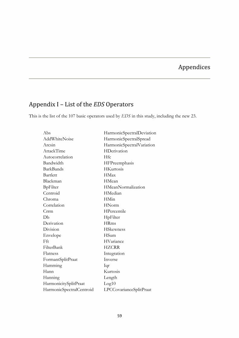
59
Appendices
Appendix I – List of the EDS Operators This is the list of the 107 basic operators used by EDS in this study, including the new 23.
Abs HarmonicSpectralDeviation AddWhiteNoise HarmonicSpectralSpread Arcsin HarmonicSpectralVariation AttackTime HDerivation Autocorrelation Hfc Bandwidth HFPreemphasis BarkBands HKurtosis Bartlett HMax Blackman HMean BpFilter HMeanNormalization Centroid HMedian Chroma HMin Correlation HNorm Crrm HPercentile Db HpFilter Derivation HRms Division HSkewness Envelope HSum Fft HVariance FilterBank HZCRR Flatness Integration FormantSplitPraat Inverse Hamming Iqr Hann Kurtosis Hanning Length HarmonicitySplitPraat Log10 HarmonicSpectralCentroid LPCCovarianceSplitPraat

Appendices
60
LPCResidualError PointProcessPraat LpFilter Power LRMSR Range LSTER RegressionCoeffs LtasPCPraat RemoveSilentFrames LtasPraat Rhf Max Rms MaxPos Skewness Mean SpectralCentroid Median SpectralDecrease MelBands SpectralFlatness MelFilterBank SpectralKurtosis Mfcc SpectralRolloff Mfcc0 SpectralSkewness Min SpectralSpread ModulationEnergy Split Multiplication SplitOverlap Norm Sqrt Normalize Square Nth Sum NthColumns Triangle PeakPos TwelveTones Peaks Variance Percentile VMeanNormalization Pitch VRegressionCoeffs PitchBands Zcr PitchSplitPraat
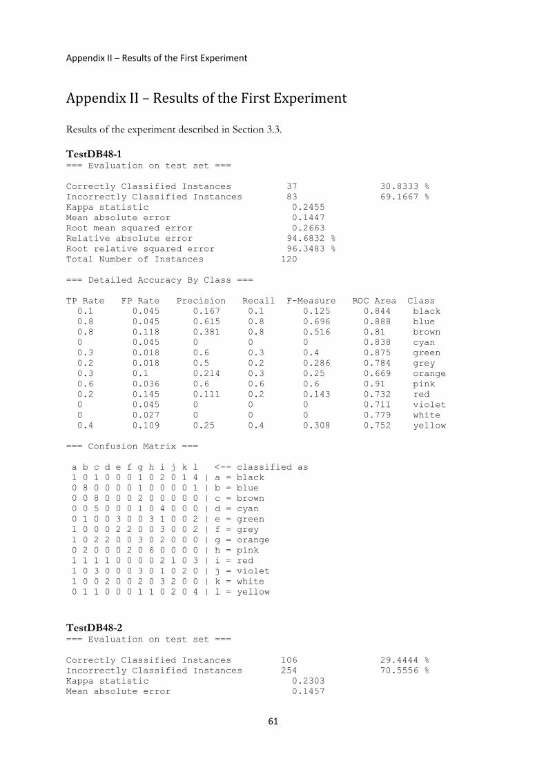
Appendix II – Results of the First Experiment
61
Appendix II – Results of the First Experiment Results of the experiment described in Section 3.3. TestDB48-1 === Evaluation on test set === Correctly Classified Instances 37 30.8333 % Incorrectly Classified Instances 83 69.1667 % Kappa statistic 0.2455 Mean absolute error 0.1447 Root mean squared error 0.2663 Relative absolute error 94.6832 % Root relative squared error 96.3483 % Total Number of Instances 120 === Detailed Accuracy By Class === TP Rate FP Rate Precision Recall F-Measure ROC Area Class 0.1 0.045 0.167 0.1 0.125 0.844 black 0.8 0.045 0.615 0.8 0.696 0.888 blue 0.8 0.118 0.381 0.8 0.516 0.81 brown 0 0.045 0 0 0 0.838 cyan 0.3 0.018 0.6 0.3 0.4 0.875 green 0.2 0.018 0.5 0.2 0.286 0.784 grey 0.3 0.1 0.214 0.3 0.25 0.669 orange 0.6 0.036 0.6 0.6 0.6 0.91 pink 0.2 0.145 0.111 0.2 0.143 0.732 red 0 0.045 0 0 0 0.711 violet 0 0.027 0 0 0 0.779 white 0.4 0.109 0.25 0.4 0.308 0.752 yellow === Confusion Matrix === a b c d e f g h i j k l <-- classified as 1 0 1 0 0 0 1 0 2 0 1 4 | a = black 0 8 0 0 0 0 1 0 0 0 0 1 | b = blue 0 0 8 0 0 0 2 0 0 0 0 0 | c = brown 0 0 5 0 0 0 1 0 4 0 0 0 | d = cyan 0 1 0 0 3 0 0 3 1 0 0 2 | e = green 1 0 0 0 2 2 0 0 3 0 0 2 | f = grey 1 0 2 2 0 0 3 0 2 0 0 0 | g = orange 0 2 0 0 0 2 0 6 0 0 0 0 | h = pink 1 1 1 1 0 0 0 0 2 1 0 3 | i = red 1 0 3 0 0 0 3 0 1 0 2 0 | j = violet 1 0 0 2 0 0 2 0 3 2 0 0 | k = white 0 1 1 0 0 0 1 1 0 2 0 4 | l = yellow TestDB48-2 === Evaluation on test set === Correctly Classified Instances 106 29.4444 % Incorrectly Classified Instances 254 70.5556 % Kappa statistic 0.2303 Mean absolute error 0.1457
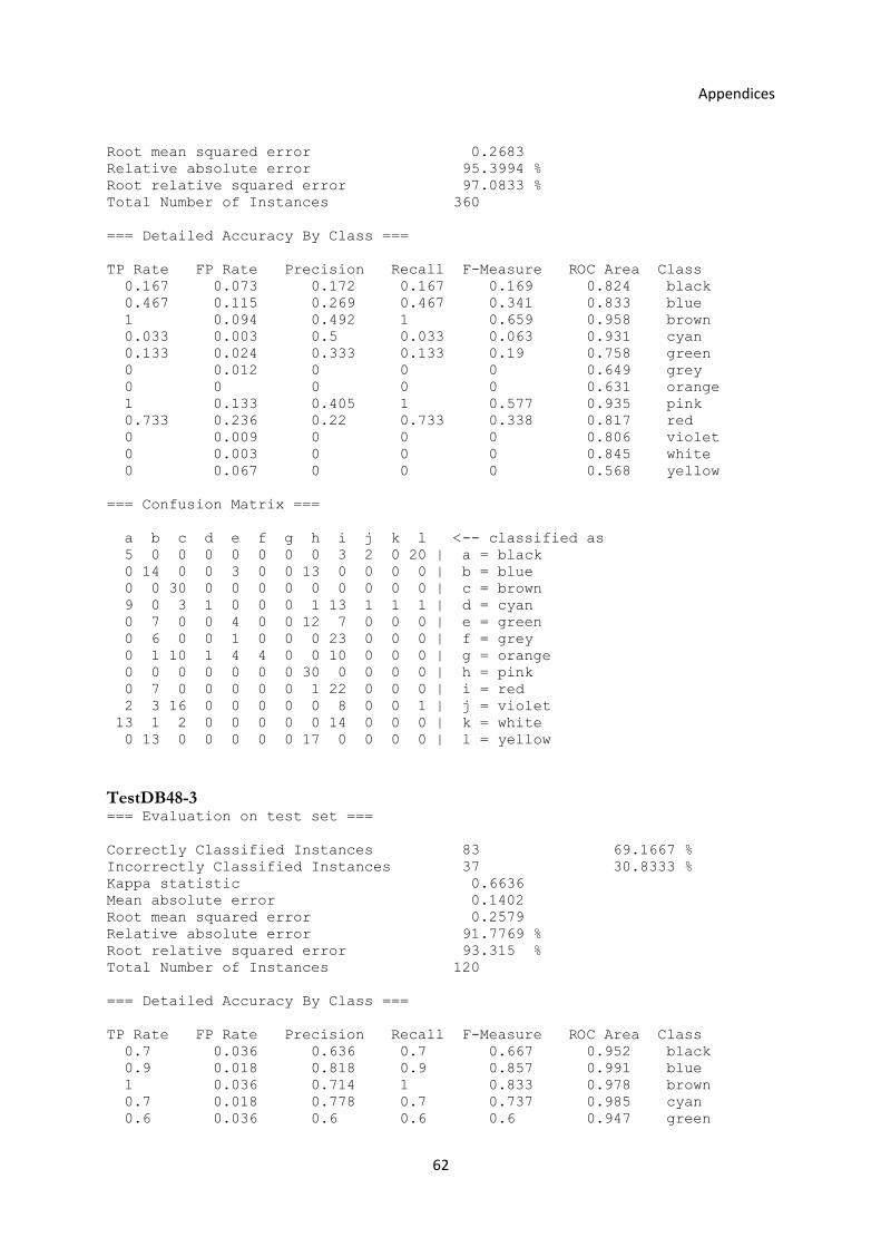
Appendices
62
Root mean squared error 0.2683 Relative absolute error 95.3994 % Root relative squared error 97.0833 % Total Number of Instances 360 === Detailed Accuracy By Class === TP Rate FP Rate Precision Recall F-Measure ROC Area Class 0.167 0.073 0.172 0.167 0.169 0.824 black 0.467 0.115 0.269 0.467 0.341 0.833 blue 1 0.094 0.492 1 0.659 0.958 brown 0.033 0.003 0.5 0.033 0.063 0.931 cyan 0.133 0.024 0.333 0.133 0.19 0.758 green 0 0.012 0 0 0 0.649 grey 0 0 0 0 0 0.631 orange 1 0.133 0.405 1 0.577 0.935 pink 0.733 0.236 0.22 0.733 0.338 0.817 red 0 0.009 0 0 0 0.806 violet 0 0.003 0 0 0 0.845 white 0 0.067 0 0 0 0.568 yellow === Confusion Matrix === a b c d e f g h i j k l <-- classified as 5 0 0 0 0 0 0 0 3 2 0 20 | a = black 0 14 0 0 3 0 0 13 0 0 0 0 | b = blue 0 0 30 0 0 0 0 0 0 0 0 0 | c = brown 9 0 3 1 0 0 0 1 13 1 1 1 | d = cyan 0 7 0 0 4 0 0 12 7 0 0 0 | e = green 0 6 0 0 1 0 0 0 23 0 0 0 | f = grey 0 1 10 1 4 4 0 0 10 0 0 0 | g = orange 0 0 0 0 0 0 0 30 0 0 0 0 | h = pink 0 7 0 0 0 0 0 1 22 0 0 0 | i = red 2 3 16 0 0 0 0 0 8 0 0 1 | j = violet 13 1 2 0 0 0 0 0 14 0 0 0 | k = white 0 13 0 0 0 0 0 17 0 0 0 0 | l = yellow TestDB48-3 === Evaluation on test set === Correctly Classified Instances 83 69.1667 % Incorrectly Classified Instances 37 30.8333 % Kappa statistic 0.6636 Mean absolute error 0.1402 Root mean squared error 0.2579 Relative absolute error 91.7769 % Root relative squared error 93.315 % Total Number of Instances 120 === Detailed Accuracy By Class === TP Rate FP Rate Precision Recall F-Measure ROC Area Class 0.7 0.036 0.636 0.7 0.667 0.952 black 0.9 0.018 0.818 0.9 0.857 0.991 blue 1 0.036 0.714 1 0.833 0.978 brown 0.7 0.018 0.778 0.7 0.737 0.985 cyan 0.6 0.036 0.6 0.6 0.6 0.947 green
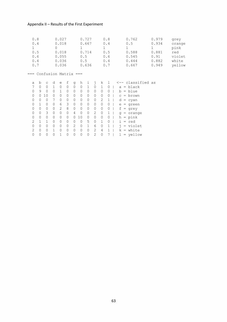
Appendix II – Results of the First Experiment
63
0.8 0.027 0.727 0.8 0.762 0.979 grey 0.4 0.018 0.667 0.4 0.5 0.934 orange 1 0 1 1 1 1 pink 0.5 0.018 0.714 0.5 0.588 0.881 red 0.6 0.055 0.5 0.6 0.545 0.91 violet 0.4 0.036 0.5 0.4 0.444 0.882 white 0.7 0.036 0.636 0.7 0.667 0.949 yellow === Confusion Matrix === a b c d e f g h i j k l <-- classified as 7 0 0 1 0 0 0 0 1 0 1 0 | a = black 0 9 0 0 1 0 0 0 0 0 0 0 | b = blue 0 0 10 0 0 0 0 0 0 0 0 0 | c = brown 0 0 0 7 0 0 0 0 0 0 2 1 | d = cyan 0 1 0 0 6 3 0 0 0 0 0 0 | e = green 0 0 0 0 2 8 0 0 0 0 0 0 | f = grey 0 0 3 0 0 0 4 0 0 2 0 1 | g = orange 0 0 0 0 0 0 0 10 0 0 0 0 | h = pink 2 1 1 0 0 0 0 0 5 0 1 0 | i = red 0 0 0 0 0 0 2 0 1 6 0 1 | j = violet 2 0 0 1 0 0 0 0 0 2 4 1 | k = white 0 0 0 0 1 0 0 0 0 2 0 7 | l = yellow

Appendices
64
Appendix III – Matlab® Code of the Endpoint Detector This is the Matlab® code of the endpoint detector presented in Section 3.4. The code consists of 5 functions: EndpointDetector, LPCdecision, Startpointposition, Findmaxima and Findminima. function EndpointDetector(filename) % ENDPOINTDETECTOR % Given a .wav filename containing an isolated utterance, this function % finds the start and endpoints of the utterance and creates a new % .wav file in a folder named "cut" % with the same utterance without the silence or noises surrounding it, % even in low SNR conditions. % Estimation is done thanks to the computation frame per frame of % the variance of the prediction error of LPC. % % If FILENAME is a name of a folder, ENDPOINTDETECTOR computes % the function recursively on all .wav files contained in the % folder or subfolders. % % Parameters and things to play with: % % In variance of the error computation: % bypassing preemphasis filter % bypassing hamming windowing % frame length (Tf) % AR model order (P) % overlap percentage (overlap) % frame normalisation % % In the startpoint/endpoint decision: % upper and lower nominal threshold for the error variance (uTh, lTh) % smoothing order (sorder) % % Gonçal Calvo, July 2008 % Read the audio files % -------------------- newdir_shortname = 'cut'; if (isdir(filename)) vectFile = dir(filename); for ind = 1 : size(vectFile, 1) filen = vectFile(ind).name; if (~strcmp(filen(1 : 1), '.')& ~strcmp(filen, newdir_shortname)) filen = strcat(filename, '\', filen); EndpointDetector(filen); end end end if (strcmp(filename(size(filename, 2)-3 : size(filename, 2)), '.wav')) fprintf('Treating %s\n', filename); else fprintf('##Not a wavfile %s\n', filename); return; end
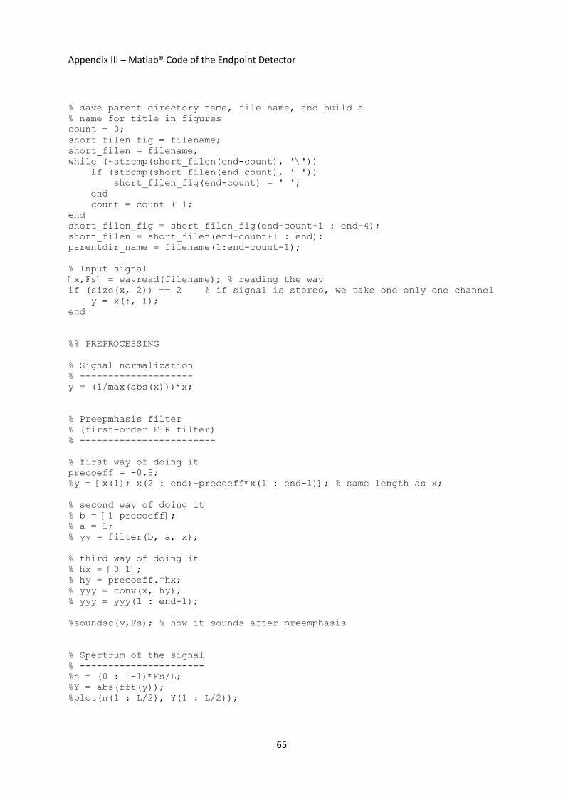
Appendix III – Matlab® Code of the Endpoint Detector
65
% save parent directory name, file name, and build a % name for title in figures count = 0; short_filen_fig = filename; short_filen = filename; while (~strcmp(short_filen(end-count), '\')) if (strcmp(short_filen(end-count), '_')) short_filen_fig(end-count) = ' '; end count = count + 1; end short_filen_fig = short_filen_fig(end-count+1 : end-4); short_filen = short_filen(end-count+1 : end); parentdir_name = filename(1:end-count-1); % Input signal [x,Fs] = wavread(filename); % reading the wav if (size(x, 2)) == 2 % if signal is stereo, we take one only one channel y = x(:, 1); end %% PREPROCESSING % Signal normalization % -------------------- y = (1/max(abs(x)))*x; % Preepmhasis filter % (first-order FIR filter) % ------------------------ % first way of doing it precoeff = -0.8; %y = [x(1); x(2 : end)+precoeff*x(1 : end-1)]; % same length as x; % second way of doing it % b = [1 precoeff]; % a = 1; % yy = filter(b, a, x); % third way of doing it % hx = [0 1]; % hy = precoeff.^hx; % yyy = conv(x, hy); % yyy = yyy(1 : end-1); %soundsc(y,Fs); % how it sounds after preemphasis % Spectrum of the signal % ---------------------- %n = (0 : L-1)*Fs/L; %Y = abs(fft(y)); %plot(n(1 : L/2), Y(1 : L/2));

Appendices
66
% White noise addition % -------------------- %wn = 0.001*randn(length(y), 1); % white noise addition %y = y + wn; % Low-pass filtering % ------------------ [b_lp, a_lp] = ellip(6, 3, 40, 300/Fs, 'high'); y = filter(b_lp, a_lp, y); %% END OF PREPROCESSING % Computing decision curve (prediction error variance) % ---------------------------------------------------- %% Parameters: Tf = 0.01; % length of a frame in seconds (normally 20ms % for speech prediction) Lf = ceil(Tf*Fs); % length of a frame in samples overlap = 0.75; % amount of frame overlapping P = 10; % AR model order R = ceil((1-overlap)*Lf); % frame step (hop size) (in samples) %% Computing the decision curve for Startpoint [logvare_v, ep_v] = LPCdecision(y, Lf, overlap, P); % it returns a %vector with the variance of the prediction error (in log) of each %analysis frame, and the prediction error vector %soundsc(ep_v,Fs) %plot(log(abs(ep_v))) sorder = 20; % smoothing the curve a1 = 1; b1 = (1/sorder)*ones(1, sorder); logvaref_v = filtfilt(b1, a1, logvare_v); % smoothed logvare_v %% Computing the decision curve for Endpoint yrev = y(end : -1 : 1); % first the signal must be reversed % the computation is then the same as for the Startpoint: [logvarerev_v, eprev_v] = LPCdecision(yrev, Lf, overlap, P); logvarerevf_v = filtfilt(b1, a1, logvarerev_v); % smoothed logvarerev_v % Computation of the Startpoint and Endpoint positions % ---------------------------------------------------- % Thresholds % logvaref_v's ceil mavmax = max(logvaref_v(ceil(sorder/2):floor(end-sorder/2))); % logvaref_v's floor mavmin = min(logvaref_v); % nominal upper threshold for the error variance uTh = (mavmin-mavmax)*0.1 + mavmax; % nominal lower threshold for the error variance lTh = (mavmin-mavmax)*0.25 + mavmax; %% Startpoint decision wstart = Startpointposition(logvaref_v, uTh, lTh);
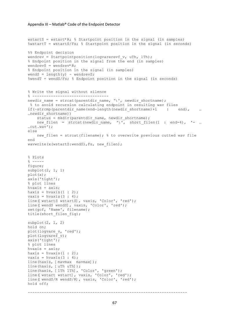
Appendix III – Matlab® Code of the Endpoint Detector
67
wstartS = wstart*R; % Startpoint position in the signal (in samples) %wstartT = wstartS/Fs; % Startpoint position in the signal (in seconds) %% Endpoint decision wendrev = Startpointposition(logvarerevf_v, uTh, lTh); % Endpoint position in the signal from the end (in samples) wendrevS = wendrev*R; % Endpoint position in the signal (in samples) wendS = length(y) - wendrevS; %wendT = wendS/Fs; % Endpoint position in the signal (in seconds) % Write the signal without silence % --------------------------------- newdir_name = strcat(parentdir_name, '\', newdir_shortname); % to avoid recursion calculating endpoint in resulting wav files if(~strcmp(parentdir_name(end-length(newdir_shortname)+1 : end), … …newdir_shortname)) status = mkdir(parentdir_name, newdir_shortname); new_filen = strcat(newdir_name, '\', short_filen(1 : end-4), '- … …cut.wav'); else new_filen = strcat(filename); % to overwrite previous cutted wav file end wavwrite(x(wstartS:wendS),Fs, new_filen); % Plots % ----- figure; subplot(2, 1, 1) plot(x); axis('tight'); % plot lines hvaxis = axis; haxis = hvaxis(1 : 2); vaxis = hvaxis(3 : 4); line([wstartS wstartS], vaxis, 'Color', 'red'); line([wendS wendS], vaxis, 'Color', 'red'); set(gcf, 'Name', filename); title(short_filen_fig); subplot(2, 1, 2) hold on; plot(logvare_v, 'red'); plot(logvaref_v); axis('tight'); % plot lines hvaxis = axis; haxis = hvaxis(1 : 2); vaxis = hvaxis(3 : 4); line(haxis, [mavmax mavmax]); line(haxis, [uTh uTh]); line(haxis, [lTh lTh], 'Color', 'green'); line([wstart wstart], vaxis, 'Color', 'red'); line([wendS/R wendS/R], vaxis, 'Color', 'red'); hold off; ---------------------------------------------------------------------
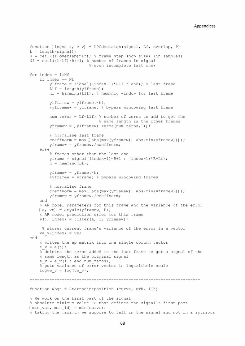
Appendices
68
function [logve_v, e_v] = LPCdecision(signal, Lf, overlap, P) L = length(signal); R = ceil((1-overlap)*Lf); % frame step (hop size) (in samples) Nf = ceil((L-Lf)/R)+1; % number of frames in signal %(even incomplete last one) for index = 1:Nf if index == Nf ylframe = signal((index-1)*R+1 : end); % last frame Llf = length(ylframe); hl = hamming(Llf); % hammnig window for last frame ylframew = ylframe.*hl; %ylframew = ylframe; % bypass windowing last frame num_zeros = Lf-Llf; % number of zeros to add to get the % same length as the other frames yframew = [ylframew; zeros(num_zeros,1)]; % normalise last frame coeffnorm = max([abs(max(yframew)) abs(min(yframew))]); yframew = yframew./coeffnorm; else % frames other than the last one yframe = signal((index-1)*R+1 : (index-1)*R+Lf); h = hamming(Lf); yframew = yframe.*h; %yframew = yframe; % bypass windowing frames % normalise frame coeffnorm = max([abs(max(yframew)) abs(min(yframew))]); yframew = yframew./coeffnorm; end % AR model parameters for this frame and the variance of the error [a, ve] = aryule(yframew, P); % AR model prediction error for this frame e(:, index) = filter(a, 1, yframew); % stores current frame's variance of the error in a vector ve_v(index) = ve; end % writes the ep matrix into one single column vector e_v = e(:); % deletes the zeros added in the last frame to get a signal of the % same length as the original signal e_v = e_v(1 : end-num_zeros); % puts variance of error vector in logarithmic scale logve_v = log(ve_v); --------------------------------------------------------------------- function wbgn = Startpointposition (curve, uTh, lTh) % We work on the first part of the signal % absolute minimum value -> that defines the signal's first part [min_val, min_id] = min(curve); % taking the maximum we suppose to fall in the signal and not in a spurious
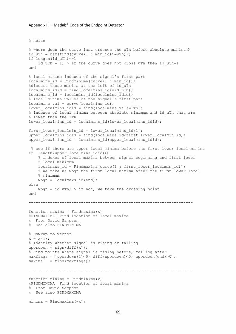
Appendix III – Matlab® Code of the Endpoint Detector
69
% noise % where does the curve last crosses the uTh before absolute minimum? id_uTh = max(find(curve(1 : min_id)>=uTh)); if length(id_uTh)~=1 id_uTh = 1; % if the curve does not cross uTh then id_uTh=1 end % local minima indexes of the signal's first part localmins_id = Findminima(curve(1 : min_id)); %discart those minima at the left of id_uTh localmins_idid = find(localmins_id>=id_uTh); localmins_id = localmins_id(localmins_idid); % local minima values of the signal's first part localmins_val = curve(localmins_id); lower_localmins_idid = find(localmins_val<=lTh); % indexes of local minima between absolute minimum and id_uTh that are % lower than the lTh lower_localmins_id = localmins_id(lower_localmins_idid); first_lower_localmin_id = lower_localmins_id(1); upper_localmins_idid = find(localmins_id<first_lower_localmin_id); upper_localmins_id = localmins_id(upper_localmins_idid); % see if there are upper local minima before the first lower local minima if length(upper_localmins_idid)>0 % indexes of local maxima between signal beginning and first lower % local minimum localmaxs_id = Findmaxima(curve(1 : first_lower_localmin_id)); % we take as wbgn the first local maxima after the first lower local % minimum wbgn = localmaxs_id(end); else wbgn = id_uTh; % if not, we take the crossing point end --------------------------------------------------------------------- function maxima = Findmaxima(x) %FINDMAXIMA Find location of local maxima % From David Sampson % See also FINDMINIMA % Unwrap to vector x = x(:); % Identify whether signal is rising or falling upordown = sign(diff(x)); % Find points where signal is rising before, falling after maxflags = [upordown(1)<0; diff(upordown)<0; upordown(end)>0]; maxima = find(maxflags); --------------------------------------------------------------------- function minima = Findminima(x) %FINDMINIMA Find location of local minima % From David Sampson % See also FINDMAXIMA minima = Findmaxima(-x);
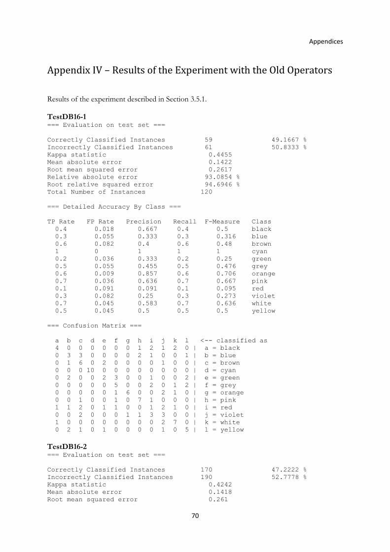
Appendices
70
Appendix IV – Results of the Experiment with the Old Operators Results of the experiment described in Section 3.5.1. TestDB16-1 === Evaluation on test set === Correctly Classified Instances 59 49.1667 % Incorrectly Classified Instances 61 50.8333 % Kappa statistic 0.4455 Mean absolute error 0.1422 Root mean squared error 0.2617 Relative absolute error 93.0854 % Root relative squared error 94.6946 % Total Number of Instances 120 === Detailed Accuracy By Class === TP Rate FP Rate Precision Recall F-Measure Class 0.4 0.018 0.667 0.4 0.5 black 0.3 0.055 0.333 0.3 0.316 blue 0.6 0.082 0.4 0.6 0.48 brown 1 0 1 1 1 cyan 0.2 0.036 0.333 0.2 0.25 green 0.5 0.055 0.455 0.5 0.476 grey 0.6 0.009 0.857 0.6 0.706 orange 0.7 0.036 0.636 0.7 0.667 pink 0.1 0.091 0.091 0.1 0.095 red 0.3 0.082 0.25 0.3 0.273 violet 0.7 0.045 0.583 0.7 0.636 white 0.5 0.045 0.5 0.5 0.5 yellow === Confusion Matrix === a b c d e f g h i j k l <-- classified as 4 0 0 0 0 0 0 1 2 1 2 0 | a = black 0 3 3 0 0 0 0 2 1 0 0 1 | b = blue 0 1 6 0 2 0 0 0 0 1 0 0 | c = brown 0 0 0 10 0 0 0 0 0 0 0 0 | d = cyan 0 2 0 0 2 3 0 0 1 0 0 2 | e = green 0 0 0 0 0 5 0 0 2 0 1 2 | f = grey 0 0 0 0 0 1 6 0 0 2 1 0 | g = orange 0 0 1 0 0 1 0 7 1 0 0 0 | h = pink 1 1 2 0 1 1 0 0 1 2 1 0 | i = red 0 0 2 0 0 0 1 1 3 3 0 0 | j = violet 1 0 0 0 0 0 0 0 0 2 7 0 | k = white 0 2 1 0 1 0 0 0 0 1 0 5 | l = yellow TestDB16-2 === Evaluation on test set === Correctly Classified Instances 170 47.2222 % Incorrectly Classified Instances 190 52.7778 % Kappa statistic 0.4242 Mean absolute error 0.1418 Root mean squared error 0.261
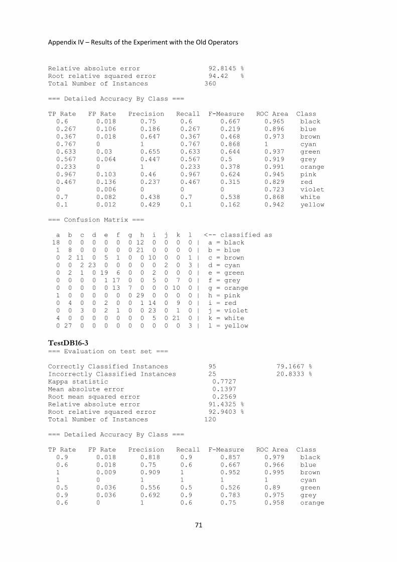
Appendix IV – Results of the Experiment with the Old Operators
71
Relative absolute error 92.8145 % Root relative squared error 94.42 % Total Number of Instances 360 === Detailed Accuracy By Class === TP Rate FP Rate Precision Recall F-Measure ROC Area Class 0.6 0.018 0.75 0.6 0.667 0.965 black 0.267 0.106 0.186 0.267 0.219 0.896 blue 0.367 0.018 0.647 0.367 0.468 0.973 brown 0.767 0 1 0.767 0.868 1 cyan 0.633 0.03 0.655 0.633 0.644 0.937 green 0.567 0.064 0.447 0.567 0.5 0.919 grey 0.233 0 1 0.233 0.378 0.991 orange 0.967 0.103 0.46 0.967 0.624 0.945 pink 0.467 0.136 0.237 0.467 0.315 0.829 red 0 0.006 0 0 0 0.723 violet 0.7 0.082 0.438 0.7 0.538 0.868 white 0.1 0.012 0.429 0.1 0.162 0.942 yellow === Confusion Matrix === a b c d e f g h i j k l <-- classified as 18 0 0 0 0 0 0 12 0 0 0 0 | a = black 1 8 0 0 0 0 0 21 0 0 0 0 | b = blue 0 2 11 0 5 1 0 0 10 0 0 1 | c = brown 0 0 2 23 0 0 0 0 0 2 0 3 | d = cyan 0 2 1 0 19 6 0 0 2 0 0 0 | e = green 0 0 0 0 1 17 0 0 5 0 7 0 | f = grey 0 0 0 0 0 13 7 0 0 0 10 0 | g = orange 1 0 0 0 0 0 0 29 0 0 0 0 | h = pink 0 4 0 0 2 0 0 1 14 0 9 0 | i = red 0 0 3 0 2 1 0 0 23 0 1 0 | j = violet 4 0 0 0 0 0 0 0 5 0 21 0 | k = white 0 27 0 0 0 0 0 0 0 0 0 3 | l = yellow TestDB16-3 === Evaluation on test set === Correctly Classified Instances 95 79.1667 % Incorrectly Classified Instances 25 20.8333 % Kappa statistic 0.7727 Mean absolute error 0.1397 Root mean squared error 0.2569 Relative absolute error 91.4325 % Root relative squared error 92.9403 % Total Number of Instances 120 === Detailed Accuracy By Class === TP Rate FP Rate Precision Recall F-Measure ROC Area Class 0.9 0.018 0.818 0.9 0.857 0.979 black 0.6 0.018 0.75 0.6 0.667 0.966 blue 1 0.009 0.909 1 0.952 0.995 brown 1 0 1 1 1 1 cyan 0.5 0.036 0.556 0.5 0.526 0.89 green 0.9 0.036 0.692 0.9 0.783 0.975 grey 0.6 0 1 0.6 0.75 0.958 orange
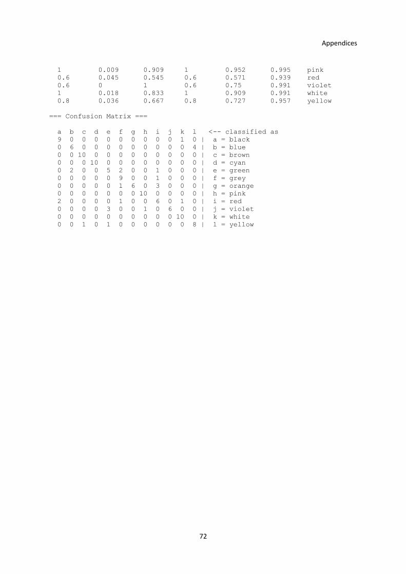
Appendices
72
1 0.009 0.909 1 0.952 0.995 pink 0.6 0.045 0.545 0.6 0.571 0.939 red 0.6 0 1 0.6 0.75 0.991 violet 1 0.018 0.833 1 0.909 0.991 white 0.8 0.036 0.667 0.8 0.727 0.957 yellow === Confusion Matrix === a b c d e f g h i j k l <-- classified as 9 0 0 0 0 0 0 0 0 0 1 0 | a = black 0 6 0 0 0 0 0 0 0 0 0 4 | b = blue 0 0 10 0 0 0 0 0 0 0 0 0 | c = brown 0 0 0 10 0 0 0 0 0 0 0 0 | d = cyan 0 2 0 0 5 2 0 0 1 0 0 0 | e = green 0 0 0 0 0 9 0 0 1 0 0 0 | f = grey 0 0 0 0 0 1 6 0 3 0 0 0 | g = orange 0 0 0 0 0 0 0 10 0 0 0 0 | h = pink 2 0 0 0 0 1 0 0 6 0 1 0 | i = red 0 0 0 0 3 0 0 1 0 6 0 0 | j = violet 0 0 0 0 0 0 0 0 0 0 10 0 | k = white 0 0 1 0 1 0 0 0 0 0 0 8 | l = yellow

Appendix V – Results of the Experiment with the Old and New Operators
73
Appendix V – Results of the Experiment with the Old and New Operators Results of the experiment described in Section 3.5.2. TestDB16-1 === Evaluation on test set === Correctly Classified Instances 68 56.6667 % Incorrectly Classified Instances 52 43.3333 % Kappa statistic 0.5273 Mean absolute error 0.1418 Root mean squared error 0.2608 Relative absolute error 92.7824 % Root relative squared error 94.3745 % Total Number of Instances 120 === Detailed Accuracy By Class === TP Rate FP Rate Precision Recall F-Measure Class 0.4 0.018 0.667 0.4 0.5 black 0.3 0.091 0.231 0.3 0.261 blue 0.8 0.036 0.667 0.8 0.727 brown 0.8 0 1 0.8 0.889 cyan 0.4 0.064 0.364 0.4 0.381 green 0.4 0.027 0.571 0.4 0.471 grey 0.8 0.036 0.667 0.8 0.727 orange 0.8 0 1 0.8 0.889 pink 0.3 0.018 0.6 0.3 0.4 red 0.5 0.082 0.357 0.5 0.417 violet 0.5 0.045 0.5 0.5 0.5 white 0.8 0.055 0.571 0.8 0.667 yellow === Confusion Matrix === a b c d e f g h i j k l <-- classified as 4 0 1 0 0 0 0 0 0 4 1 0 | a = black 0 3 3 0 0 0 0 0 0 0 0 4 | b = blue 0 0 8 0 0 0 0 0 0 0 0 2 | c = brown 0 0 0 8 2 0 0 0 0 0 0 0 | d = cyan 0 2 0 0 4 2 0 0 0 2 0 0 | e = green 0 0 0 0 1 4 0 0 2 2 1 0 | f = grey 0 0 0 0 0 0 8 0 0 0 2 0 | g = orange 0 1 0 0 1 0 0 8 0 0 0 0 | h = pink 2 4 0 0 1 0 0 0 3 0 0 0 | i = red 0 1 0 0 2 0 1 0 0 5 1 0 | j = violet 0 0 0 0 0 1 3 0 0 1 5 0 | k = white 0 2 0 0 0 0 0 0 0 0 0 8 | l = yellow TestDB16-2 === Evaluation on test set === Correctly Classified Instances 224 62.2222 % Incorrectly Classified Instances 136 37.7778 % Kappa statistic 0.5879
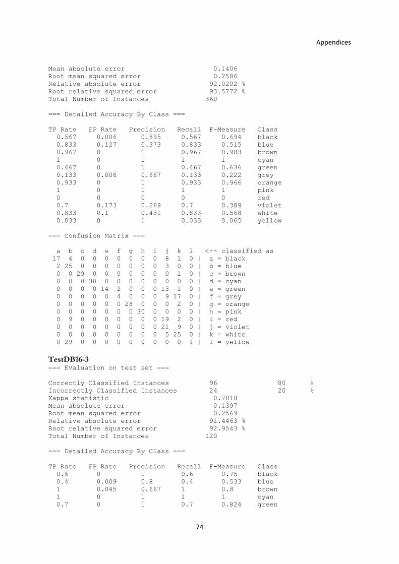
Appendices
74
Mean absolute error 0.1406 Root mean squared error 0.2586 Relative absolute error 92.0202 % Root relative squared error 93.5772 % Total Number of Instances 360 === Detailed Accuracy By Class === TP Rate FP Rate Precision Recall F-Measure Class 0.567 0.006 0.895 0.567 0.694 black 0.833 0.127 0.373 0.833 0.515 blue 0.967 0 1 0.967 0.983 brown 1 0 1 1 1 cyan 0.467 0 1 0.467 0.636 green 0.133 0.006 0.667 0.133 0.222 grey 0.933 0 1 0.933 0.966 orange 1 0 1 1 1 pink 0 0 0 0 0 red 0.7 0.173 0.269 0.7 0.389 violet 0.833 0.1 0.431 0.833 0.568 white 0.033 0 1 0.033 0.065 yellow === Confusion Matrix === a b c d e f g h i j k l <-- classified as 17 4 0 0 0 0 0 0 0 8 1 0 | a = black 2 25 0 0 0 0 0 0 0 3 0 0 | b = blue 0 0 29 0 0 0 0 0 0 0 1 0 | c = brown 0 0 0 30 0 0 0 0 0 0 0 0 | d = cyan 0 0 0 0 14 2 0 0 0 13 1 0 | e = green 0 0 0 0 0 4 0 0 0 9 17 0 | f = grey 0 0 0 0 0 0 28 0 0 0 2 0 | g = orange 0 0 0 0 0 0 0 30 0 0 0 0 | h = pink 0 9 0 0 0 0 0 0 0 19 2 0 | i = red 0 0 0 0 0 0 0 0 0 21 9 0 | j = violet 0 0 0 0 0 0 0 0 0 5 25 0 | k = white 0 29 0 0 0 0 0 0 0 0 0 1 | l = yellow TestDB16-3 === Evaluation on test set === Correctly Classified Instances 96 80 % Incorrectly Classified Instances 24 20 % Kappa statistic 0.7818 Mean absolute error 0.1397 Root mean squared error 0.2569 Relative absolute error 91.4463 % Root relative squared error 92.9543 % Total Number of Instances 120 === Detailed Accuracy By Class === TP Rate FP Rate Precision Recall F-Measure Class 0.6 0 1 0.6 0.75 black 0.4 0.009 0.8 0.4 0.533 blue 1 0.045 0.667 1 0.8 brown 1 0 1 1 1 cyan 0.7 0 1 0.7 0.824 green

Appendix V – Results of the Experiment with the Old and New Operators
75
0.8 0.009 0.889 0.8 0.842 grey 0.6 0.018 0.75 0.6 0.667 orange 1 0 1 1 1 pink 1 0.045 0.667 1 0.8 red 0.7 0.027 0.7 0.7 0.7 violet 0.9 0.027 0.75 0.9 0.818 white 0.9 0.036 0.692 0.9 0.783 yellow === Confusion Matrix === a b c d e f g h i j k l <-- classified as 6 0 0 0 0 0 1 0 1 1 1 0 | a = black 0 4 3 0 0 0 0 0 0 0 0 3 | b = blue 0 0 10 0 0 0 0 0 0 0 0 0 | c = brown 0 0 0 10 0 0 0 0 0 0 0 0 | d = cyan 0 0 0 0 7 1 0 0 2 0 0 0 | e = green 0 0 0 0 0 8 0 0 0 2 0 0 | f = grey 0 0 2 0 0 0 6 0 0 0 2 0 | g = orange 0 0 0 0 0 0 0 10 0 0 0 0 | h = pink 0 0 0 0 0 0 0 0 10 0 0 0 | i = red 0 0 0 0 0 0 0 0 2 7 0 1 | j = violet 0 0 0 0 0 0 1 0 0 0 9 0 | k = white 0 1 0 0 0 0 0 0 0 0 0 9 | l = yellow
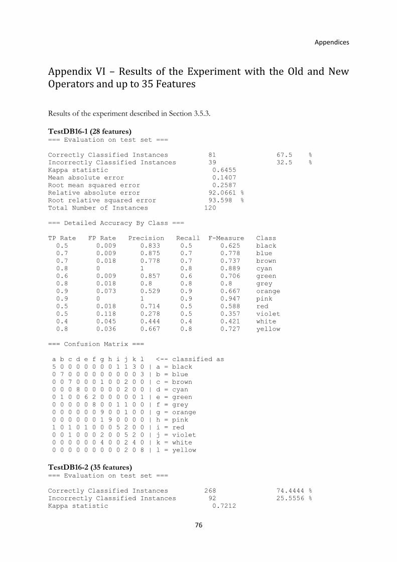
Appendices
76
Appendix VI – Results of the Experiment with the Old and New Operators and up to 35 Features Results of the experiment described in Section 3.5.3. TestDB16-1 (28 features) === Evaluation on test set === Correctly Classified Instances 81 67.5 % Incorrectly Classified Instances 39 32.5 % Kappa statistic 0.6455 Mean absolute error 0.1407 Root mean squared error 0.2587 Relative absolute error 92.0661 % Root relative squared error 93.598 % Total Number of Instances 120 === Detailed Accuracy By Class === TP Rate FP Rate Precision Recall F-Measure Class 0.5 0.009 0.833 0.5 0.625 black 0.7 0.009 0.875 0.7 0.778 blue 0.7 0.018 0.778 0.7 0.737 brown 0.8 0 1 0.8 0.889 cyan 0.6 0.009 0.857 0.6 0.706 green 0.8 0.018 0.8 0.8 0.8 grey 0.9 0.073 0.529 0.9 0.667 orange 0.9 0 1 0.9 0.947 pink 0.5 0.018 0.714 0.5 0.588 red 0.5 0.118 0.278 0.5 0.357 violet 0.4 0.045 0.444 0.4 0.421 white 0.8 0.036 0.667 0.8 0.727 yellow === Confusion Matrix === a b c d e f g h i j k l <-- classified as 5 0 0 0 0 0 0 0 1 1 3 0 | a = black 0 7 0 0 0 0 0 0 0 0 0 3 | b = blue 0 0 7 0 0 0 1 0 0 2 0 0 | c = brown 0 0 0 8 0 0 0 0 0 2 0 0 | d = cyan 0 1 0 0 6 2 0 0 0 0 0 1 | e = green 0 0 0 0 0 8 0 0 1 1 0 0 | f = grey 0 0 0 0 0 0 9 0 0 1 0 0 | g = orange 0 0 0 0 0 0 1 9 0 0 0 0 | h = pink 1 0 1 0 1 0 0 0 5 2 0 0 | i = red 0 0 1 0 0 0 2 0 0 5 2 0 | j = violet 0 0 0 0 0 0 4 0 0 2 4 0 | k = white 0 0 0 0 0 0 0 0 0 2 0 8 | l = yellow TestDB16-2 (35 features) === Evaluation on test set === Correctly Classified Instances 268 74.4444 % Incorrectly Classified Instances 92 25.5556 % Kappa statistic 0.7212
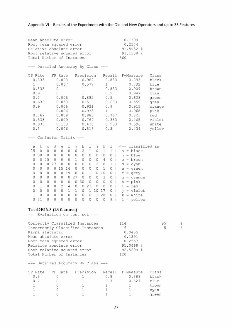
Appendix VI – Results of the Experiment with the Old and New Operators and up to 35 Features
77
Mean absolute error 0.1399 Root mean squared error 0.2574 Relative absolute error 91.5932 % Root relative squared error 93.1138 % Total Number of Instances 360 === Detailed Accuracy By Class === TP Rate FP Rate Precision Recall F-Measure Class 0.833 0.003 0.962 0.833 0.893 black 1 0.067 0.577 1 0.732 blue 0.833 0 1 0.833 0.909 brown 0.9 0 1 0.9 0.947 cyan 0.5 0.006 0.882 0.5 0.638 green 0.633 0.058 0.5 0.633 0.559 grey 0.9 0.006 0.931 0.9 0.915 orange 1 0.006 0.938 1 0.968 pink 0.767 0.009 0.885 0.767 0.821 red 0.333 0.009 0.769 0.333 0.465 violet 0.933 0.109 0.438 0.933 0.596 white 0.3 0.006 0.818 0.3 0.439 yellow === Confusion Matrix === a b c d e f g h i j k l <-- classified as 25 0 0 0 0 0 0 2 1 0 1 1 | a = black 0 30 0 0 0 0 0 0 0 0 0 0 | b = blue 0 0 25 0 0 0 1 0 0 0 4 0 | c = brown 0 0 0 27 0 0 0 0 0 2 0 1 | d = cyan 0 0 0 0 15 14 0 0 0 0 1 0 | e = green 0 0 0 0 0 19 0 0 1 0 10 0 | f = grey 0 0 0 0 0 0 27 0 0 0 3 0 | g = orange 0 0 0 0 0 0 0 30 0 0 0 0 | h = pink 0 1 0 0 2 4 0 0 23 0 0 0 | i = red 0 0 0 0 0 1 1 0 1 10 17 0 | j = violet 1 0 0 0 0 0 0 0 0 1 28 0 | k = white 0 21 0 0 0 0 0 0 0 0 0 9 | l = yellow TestDB16-3 (23 features) === Evaluation on test set === Correctly Classified Instances 114 95 % Incorrectly Classified Instances 6 5 % Kappa statistic 0.9455 Mean absolute error 0.1391 Root mean squared error 0.2557 Relative absolute error 91.0468 % Root relative squared error 92.5299 % Total Number of Instances 120 === Detailed Accuracy By Class === TP Rate FP Rate Precision Recall F-Measure Class 0.8 0 1 0.8 0.889 black 0.7 0 1 0.7 0.824 blue 1 0 1 1 1 brown 1 0 1 1 1 cyan 1 0 1 1 1 green
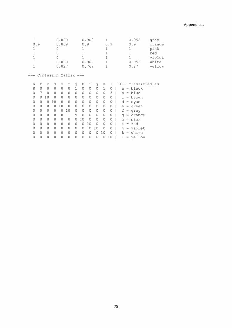
Appendices
78
1 0.009 0.909 1 0.952 grey 0.9 0.009 0.9 0.9 0.9 orange 1 0 1 1 1 pink 1 0 1 1 1 red 1 0 1 1 1 violet 1 0.009 0.909 1 0.952 white 1 0.027 0.769 1 0.87 yellow === Confusion Matrix === a b c d e f g h i j k l <-- classified as 8 0 0 0 0 0 1 0 0 0 1 0 | a = black 0 7 0 0 0 0 0 0 0 0 0 3 | b = blue 0 0 10 0 0 0 0 0 0 0 0 0 | c = brown 0 0 0 10 0 0 0 0 0 0 0 0 | d = cyan 0 0 0 0 10 0 0 0 0 0 0 0 | e = green 0 0 0 0 0 10 0 0 0 0 0 0 | f = grey 0 0 0 0 0 1 9 0 0 0 0 0 | g = orange 0 0 0 0 0 0 0 10 0 0 0 0 | h = pink 0 0 0 0 0 0 0 0 10 0 0 0 | i = red 0 0 0 0 0 0 0 0 0 10 0 0 | j = violet 0 0 0 0 0 0 0 0 0 0 10 0 | k = white 0 0 0 0 0 0 0 0 0 0 0 10 | l = yellow
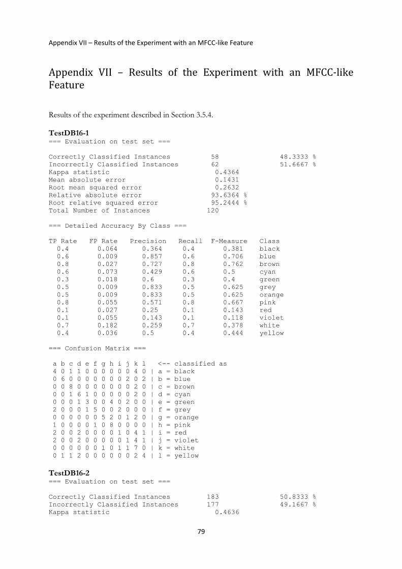
Appendix VII – Results of the Experiment with an MFCC‐like Feature
79
Appendix VII – Results of the Experiment with an MFCC‐like Feature Results of the experiment described in Section 3.5.4. TestDB16-1 === Evaluation on test set === Correctly Classified Instances 58 48.3333 % Incorrectly Classified Instances 62 51.6667 % Kappa statistic 0.4364 Mean absolute error 0.1431 Root mean squared error 0.2632 Relative absolute error 93.6364 % Root relative squared error 95.2444 % Total Number of Instances 120 === Detailed Accuracy By Class === TP Rate FP Rate Precision Recall F-Measure Class 0.4 0.064 0.364 0.4 0.381 black 0.6 0.009 0.857 0.6 0.706 blue 0.8 0.027 0.727 0.8 0.762 brown 0.6 0.073 0.429 0.6 0.5 cyan 0.3 0.018 0.6 0.3 0.4 green 0.5 0.009 0.833 0.5 0.625 grey 0.5 0.009 0.833 0.5 0.625 orange 0.8 0.055 0.571 0.8 0.667 pink 0.1 0.027 0.25 0.1 0.143 red 0.1 0.055 0.143 0.1 0.118 violet 0.7 0.182 0.259 0.7 0.378 white 0.4 0.036 0.5 0.4 0.444 yellow === Confusion Matrix === a b c d e f g h i j k l <-- classified as 4 0 1 1 0 0 0 0 0 0 4 0 | a = black 0 6 0 0 0 0 0 0 0 2 0 2 | b = blue 0 0 8 0 0 0 0 0 0 0 2 0 | c = brown 0 0 1 6 1 0 0 0 0 0 2 0 | d = cyan 0 0 0 1 3 0 0 4 0 2 0 0 | e = green 2 0 0 0 1 5 0 0 2 0 0 0 | f = grey 0 0 0 0 0 0 5 2 0 1 2 0 | g = orange 1 0 0 0 0 1 0 8 0 0 0 0 | h = pink 2 0 0 2 0 0 0 0 1 0 4 1 | i = red 2 0 0 2 0 0 0 0 0 1 4 1 | j = violet 0 0 0 0 0 0 1 0 1 1 7 0 | k = white 0 1 1 2 0 0 0 0 0 0 2 4 | l = yellow TestDB16-2 === Evaluation on test set === Correctly Classified Instances 183 50.8333 % Incorrectly Classified Instances 177 49.1667 % Kappa statistic 0.4636
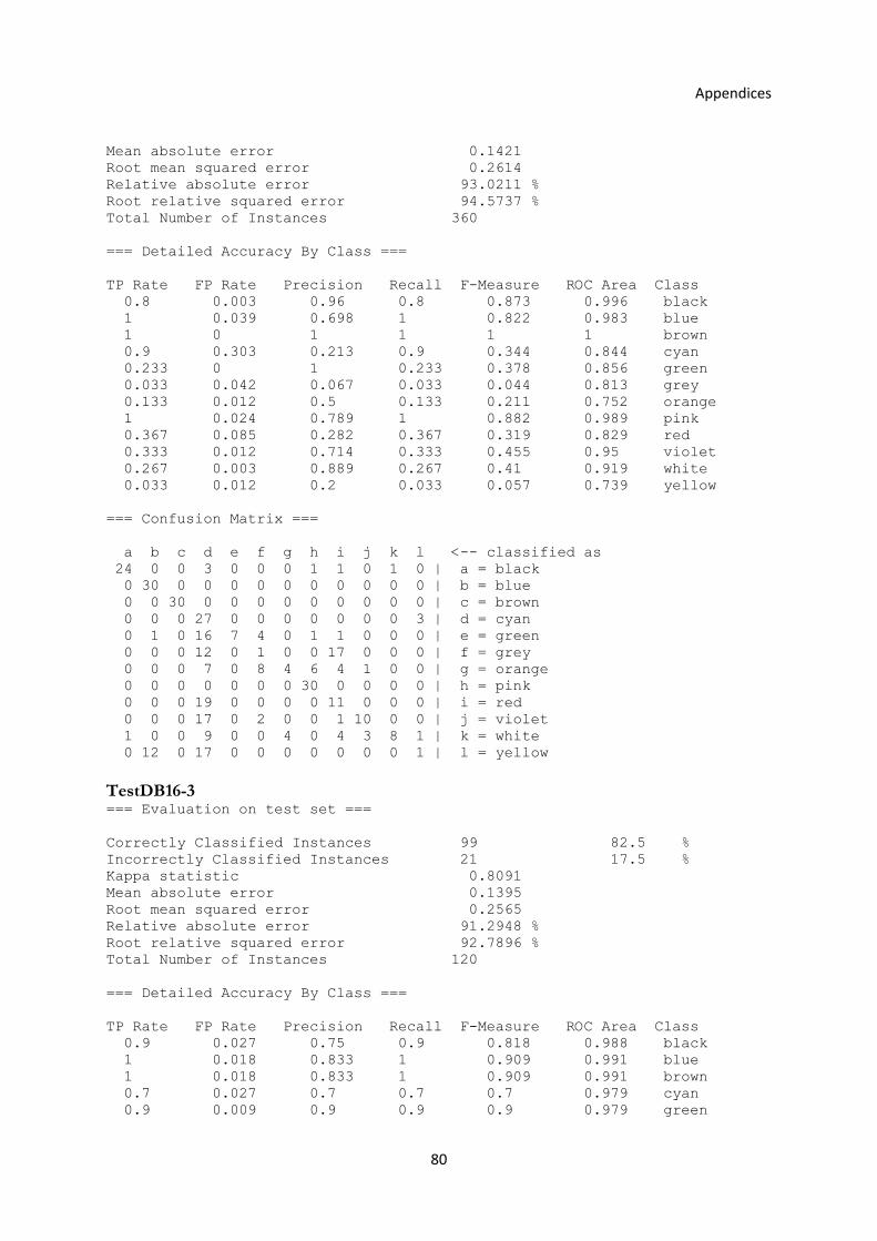
Appendices
80
Mean absolute error 0.1421 Root mean squared error 0.2614 Relative absolute error 93.0211 % Root relative squared error 94.5737 % Total Number of Instances 360 === Detailed Accuracy By Class === TP Rate FP Rate Precision Recall F-Measure ROC Area Class 0.8 0.003 0.96 0.8 0.873 0.996 black 1 0.039 0.698 1 0.822 0.983 blue 1 0 1 1 1 1 brown 0.9 0.303 0.213 0.9 0.344 0.844 cyan 0.233 0 1 0.233 0.378 0.856 green 0.033 0.042 0.067 0.033 0.044 0.813 grey 0.133 0.012 0.5 0.133 0.211 0.752 orange 1 0.024 0.789 1 0.882 0.989 pink 0.367 0.085 0.282 0.367 0.319 0.829 red 0.333 0.012 0.714 0.333 0.455 0.95 violet 0.267 0.003 0.889 0.267 0.41 0.919 white 0.033 0.012 0.2 0.033 0.057 0.739 yellow === Confusion Matrix === a b c d e f g h i j k l <-- classified as 24 0 0 3 0 0 0 1 1 0 1 0 | a = black 0 30 0 0 0 0 0 0 0 0 0 0 | b = blue 0 0 30 0 0 0 0 0 0 0 0 0 | c = brown 0 0 0 27 0 0 0 0 0 0 0 3 | d = cyan 0 1 0 16 7 4 0 1 1 0 0 0 | e = green 0 0 0 12 0 1 0 0 17 0 0 0 | f = grey 0 0 0 7 0 8 4 6 4 1 0 0 | g = orange 0 0 0 0 0 0 0 30 0 0 0 0 | h = pink 0 0 0 19 0 0 0 0 11 0 0 0 | i = red 0 0 0 17 0 2 0 0 1 10 0 0 | j = violet 1 0 0 9 0 0 4 0 4 3 8 1 | k = white 0 12 0 17 0 0 0 0 0 0 0 1 | l = yellow TestDB16-3 === Evaluation on test set === Correctly Classified Instances 99 82.5 % Incorrectly Classified Instances 21 17.5 % Kappa statistic 0.8091 Mean absolute error 0.1395 Root mean squared error 0.2565 Relative absolute error 91.2948 % Root relative squared error 92.7896 % Total Number of Instances 120 === Detailed Accuracy By Class === TP Rate FP Rate Precision Recall F-Measure ROC Area Class 0.9 0.027 0.75 0.9 0.818 0.988 black 1 0.018 0.833 1 0.909 0.991 blue 1 0.018 0.833 1 0.909 0.991 brown 0.7 0.027 0.7 0.7 0.7 0.979 cyan 0.9 0.009 0.9 0.9 0.9 0.979 green
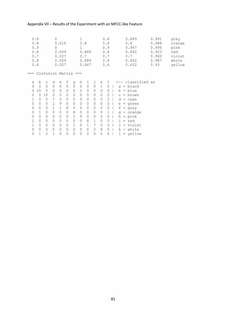
Appendix VII – Results of the Experiment with an MFCC‐like Feature
81
0.8 0 1 0.8 0.889 0.991 grey 0.8 0.018 0.8 0.8 0.8 0.988 orange 0.9 0 1 0.9 0.947 0.996 pink 0.8 0.009 0.889 0.8 0.842 0.953 red 0.7 0.027 0.7 0.7 0.7 0.962 violet 0.8 0.009 0.889 0.8 0.842 0.987 white 0.6 0.027 0.667 0.6 0.632 0.93 yellow === Confusion Matrix === a b c d e f g h i j k l <-- classified as 9 0 0 0 0 0 0 0 0 0 1 0 | a = black 0 10 0 0 0 0 0 0 0 0 0 0 | b = blue 0 0 10 0 0 0 0 0 0 0 0 0 | c = brown 1 0 0 7 0 0 0 0 0 0 0 2 | d = cyan 0 0 0 1 9 0 0 0 0 0 0 0 | e = green 0 0 0 1 1 8 0 0 0 0 0 0 | f = grey 0 1 0 0 0 0 8 0 0 0 0 1 | g = orange 0 0 0 0 0 0 1 9 0 0 0 0 | h = pink 1 0 0 0 0 0 0 0 8 1 0 0 | i = red 1 0 0 0 0 0 1 0 1 7 0 0 | j = violet 0 0 0 0 0 0 0 0 0 2 8 0 | k = white 0 1 2 1 0 0 0 0 0 0 0 6 | l = yellow