Modern Optimization Techniques · Modern Optimization Techniques 3. More on Line Search: Bold Driver Choosing the step size for SGD I The step size is a crucial parameter of gradient

Modern Optimization Techniques

Modern Optimization Techniques2. Unconstrained Optimization / 2.2. Stochastic Gradient Descent

Lars Schmidt-Thieme

Information Systems and Machine Learning Lab (ISMLL)Institute for Computer Science

University of Hildesheim, Germany

Lars Schmidt-Thieme, Information Systems and Machine Learning Lab (ISMLL), University of Hildesheim, Germany

1 / 29


Syllabus

Mon. 28.10. (0) 0. Overview

1. TheoryMon. 4.11. (1) 1. Convex Sets and Functions

2. Unconstrained OptimizationMon. 11.11. (2) 2.1 Gradient DescentMon. 18.11. (3) 2.2 Stochastic Gradient DescentMon. 25.11. (4) 2.3 Newton’s MethodMon. 2.12. (5) 2.4 Quasi-Newton MethodsMon. 19.12. (6) 2.5 Subgradient MethodsMon. 16.12. (7) 2.6 Coordinate Descent

— — Christmas Break —

3. Equality Constrained OptimizationMon. 6.1. (8) 3.1 DualityMon. 13.1. (9) 3.2 Methods

4. Inequality Constrained OptimizationMon. 20.1. (10) 4.1 Primal MethodsMon. 27.1. (11) 4.2 Barrier and Penalty MethodsMon. 3.2. (12) 4.3 Cutting Plane Methods


1 / 29


Outline

1. Stochastic Gradients

2. Stochastic Gradient Descent (SGD)

3. More on Line Search: Bold Driver

4. More on Line Search: AdaGrad


1 / 29

Modern Optimization Techniques 1. Stochastic Gradients

Outline






1 / 29


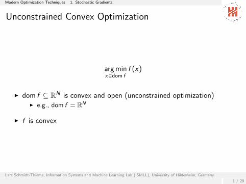
Unconstrained Convex Optimization

arg minx∈dom f

f (x)

I dom f ⊆ RN is convex and open (unconstrained optimization)I e.g., dom f = RN

I f is convex


1 / 29


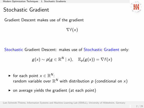
Stochastic Gradient

Gradient Descent makes use of the gradient

∇f (x)

Stochastic Gradient Descent: makes use of Stochastic Gradient only:

g(x) ∼ p(g ∈ RN | x), Ep(g(x)) = ∇f (x)

I for each point x ∈ RN :random variable over RN with distribution p (conditional on x)

I on average yields the gradient (at each point)


2 / 29


Stochastic Gradient / Example: Big Sums

f is a “big sum”:

f (x) =1

C

C∑c=1

fc(x)

with fc convex, c = 1, . . . ,C

g is the gradient of a random summand:

p(g | x) := Unif({∇fc(x) | c = 1, . . . ,C})


3 / 29


Stochastic Gradient / Example: Least Squares

minx∈RN

f (x) := ||Ax − b||22

I will find solution for Ax = b if there is any (then ||Ax − b||2 = 0)

I otherwise will find the x where the difference Ax − b of left and rightside is as small as possible (in the squared L2 norm)

I is a big sum:

f (x) := ||Ax − b||22 =M∑

m=1

((Ax)m − bm)2 =M∑

m=1

(Am,.x − bm)2

=1

M

M∑m=1

fm(x), fm(x) := M(Am,.x − bm)2

I stochastic gradient g :I gradient for a random component m


4 / 29


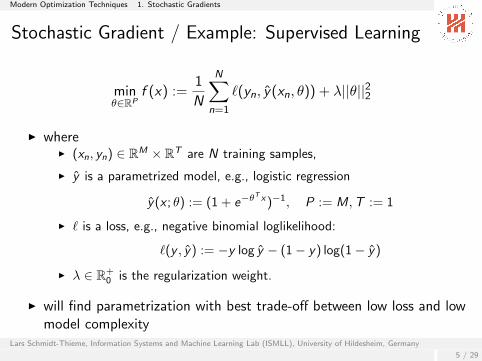
Stochastic Gradient / Example: Supervised Learning

minθ∈RP

f (x) :=1

N

N∑n=1

`(yn, y(xn, θ)) + λ||θ||22

I whereI (xn, yn) ∈ RM × RT are N training samples,

I y is a parametrized model, e.g., logistic regression

y(x ; θ) := (1 + e−θT x)−1, P := M,T := 1

I ` is a loss, e.g., negative binomial loglikelihood:

`(y , y) := −y log y − (1− y) log(1− y)

I λ ∈ R+0 is the regularization weight.

I will find parametrization with best trade-off between low loss and lowmodel complexity


5 / 29


Stochastic Gradient / Example: Supervised Learning (2/2)

minθ∈RP

f (x) :=1

N

N∑n=1

`(yn, y(xn, θ)) + λ||θ||22

I whereI (xn, yn) ∈ RM × RT are N training samples,

I . . .

I is a big sum:

f (θ) :=1

N

N∑n=1

fn(θ), fn(θ) := `(yn, y(xn, θ)) + λ||θ||22

I stochastic gradient g :I gradient for a random sample n


6 / 29

Modern Optimization Techniques 2. Stochastic Gradient Descent (SGD)

Outline






7 / 29


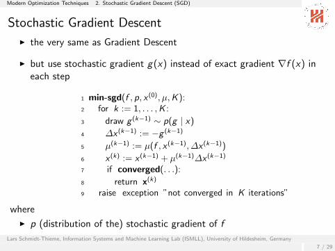
Stochastic Gradient Descent

I the very same as Gradient Descent

I but use stochastic gradient g(x) instead of exact gradient ∇f (x) ineach step

1 min-sgd(f , p, x (0), µ,K ):2 for k := 1, . . . ,K :

3 draw g (k−1) ∼ p(g | x)

4 ∆x (k−1) := −g (k−1)

5 µ(k−1) := µ(f , x (k−1), ∆x (k−1))

6 x (k) := x (k−1) + µ(k−1)∆x (k−1)

7 if converged(. . .):

8 return x(k)

9 raise exception ”not converged in K iterations”

where

I p (distribution of the) stochastic gradient of f


7 / 29


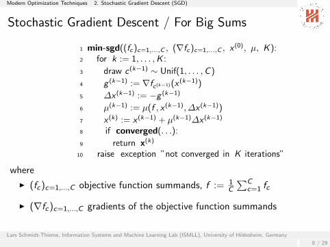
Stochastic Gradient Descent / For Big Sums

1 min-sgd((fc)c=1,...,C , (∇fc)c=1,...,C , x(0), µ, K ):

2 for k := 1, . . . ,K :

3 draw c(k−1) ∼ Unif(1, . . . ,C )

4 g (k−1) := ∇fc(k−1)(x (k−1))

5 ∆x (k−1) := −g (k−1)

6 µ(k−1) := µ(f , x (k−1), ∆x (k−1))

7 x (k) := x (k−1) + µ(k−1)∆x (k−1)

8 if converged(. . .):

9 return x(k)

10 raise exception ”not converged in K iterations”

where

I (fc)c=1,...,C objective function summands, f := 1C

∑Cc=1 fc

I (∇fc)c=1,...,C gradients of the objective function summands


8 / 29


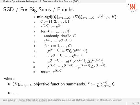
SGD / For Big Sums / Epochs1 min-sgd((fc)c=1,...,C , (∇fc)c=1,...,C , x

(0), µ, K ) :2 C := (1, 2, . . . ,C )

3 x (0,C) := x (0)

4 for k := 1, . . . ,K :5 randomly shuffle C6 x (k,0) := x (k−1,C)

7 for i = 1, . . . ,C :

8 g (k,i−1) := ∇fci (x (k,i−1))

9 ∆x (k,i−1) := −g (k,i−1)

10 µ(k,i−1) := µ(f , x (k,i−1), ∆x (k,i−1))

11 x (k,i) := x (k,i−1) + µ(k,i−1)∆x (k,i−1)

12 return x (K ,C)

whereI (fc)c=1,...,C objective function summands, f := 1

C

∑Cc=1 fc

I . . .

I K number of epochsLars Schmidt-Thieme, Information Systems and Machine Learning Lab (ISMLL), University of Hildesheim, Germany

9 / 29


Theorem (Convergence of Gradient Descent) [review]

If

(i) f is strongly convex,

(ii) the initial sublevel set S := {x ∈ dom f | f (x) ≤ f (x (0))} is closed,

(iii) an exact line search is used,

then gradient descent converges, esp.

f (x (k))− p∗ ≤ (1− m

M)k (f (x (0))− p∗)

||x (k) − x∗||2 ≤ (1− m

M)k||(∇f (x (0)))||2

m2


10 / 29


Theorem (Convergence of SGD)

If

(i) f is strongly convex (||∇2f (x)|| � mI ,m ∈ R+),

(ii) the expected squared norm of its stochastic gradient g is uniformlybounded (∃G ∈ R+

0 ∀x : E(||g(x)||2) ≤ G 2) and

(iii) the step size µ(k) := 1m(k+1) is used,

then SGD converges, esp.

Ep(||x (k) − x∗||2) ≤ 1

k + 1max{||x (0) − x∗||2, G

2

m2}


11 / 29


Convergence of SGD / Prooff (x∗)− f (x) ≥ ∇f (x)T (x∗ − x) +

m

2||x∗ − x ||2 str. conv. (i)

f (x)− f (x∗) ≥ ∇f (x∗)T (x − x∗) +m

2||x − x∗||2 =

m

2||x∗ − x ||2

summing both yields

0 ≥ ∇f (x)T (x∗ − x) + m||x∗ − x ||2

∇f (x)T (x − x∗) ≥ m||x∗ − x ||2 (1)

E(||x (k) − x∗||2)

= E(||x (k−1) − µ(k−1)g (k−1) − x∗||2)

= E(||x (k−1) − x∗||2)− 2µ(k−1)E((g (k−1))T (x (k−1) − x∗)) + (µ(k−1))2E(||gk−1||2)

= E(||x (k−1) − x∗||2)− 2µ(k−1)E(∇f (x (k−1))T (x (k−1) − x∗)) + (µ(k−1))2E(||gk−1||2)

(ii),(1)

≤ E(||x (k−1) − x∗||2)− 2µ(k−1)mE(||x∗ − x (k−1)||2) + (µ(k−1))2G 2

= (1− 2µ(k−1)m)E(||x (k−1) − x∗||2) + (µ(k−1))2G 2 (2)


12 / 29


Convergence of SGD / Proof (2/2)induction over k : k := 0:

||x (0) − x∗||2 ≤ 1

1L, L := max{||x (0) − x∗||2, G

2

m2}

k > 0:

E(||x (k) − x∗||2)(2)

≤ (1− 2µ(k−1)m)E(||x (k−1) − x∗||2) + (µ(k−1))2G 2

(iii)= (1− 2

k)E(||x (k−1) − x∗||2) +

G 2

m2k2

ind.hyp.≤ (1− 2

k)

1

kL +

G 2

m2k2

def. L≤ (1− 2

k)

1

kL +

1

k2L

=k − 2

k2L +

1

k2L =

k − 1

k2L ≤ 1

k + 1L


13 / 29

Modern Optimization Techniques 3. More on Line Search: Bold Driver

Outline






14 / 29


Choosing the step size for SGD

I The step size µ is a crucial parameter of gradient descent

I Given the low cost of the SGD update,using exact line search for the step size is a bad choice

I Possible alternatives:I Fixed step size

I Exponentially decreasing step size

I Backtracking / Armijo principle

I Bold-Driver

I Adagrad


14 / 29


Example: Body Fat predictionWe want to estimate the percentage of body fat based on variousattributes:

I Age (years)

I Weight (lbs)

I Height (inches)

I Neck circumference (cm)

I Chest circumference (cm)

I Abdomen 2 circumference (cm)

I Hip circumference (cm)

I Thigh circumference (cm)

I Knee circumference (cm)

I ...

http://lib.stat.cmu.edu/datasets/bodyfat


15 / 29

http://lib.stat.cmu.edu/datasets/bodyfat


Example: Body Fat prediction

The data is represented it as:

A =

1 a1,1 a1,2 . . . a1,M1 a2,1 a2,2 . . . a2,M...

......

......

1 aN,1 aN,2 . . . aN,M

, y =

y1y2...yN

with N = 252, M = 14

We can model the percentage of body fat yas a linear combination of the body measurements with parameters x:

yn = xTan = x01 + x1an,1 + x2an,2 + . . .+ xMan,M


16 / 29


SGD - Fixed Step Size on the Body Fat dataset

0 100 200 300 400 500

0.00

0.05

0.10

0.15

0.20

SGD Step Size

Iterations

MS

E0.00010.0010.010.1


17 / 29


Bold Driver Heuristic

I idea: use smaller step sizes closer to the minimum.

I adjust step size based on the value of f (x(k))− f (x(k−1))

I if the value of f (x) grows,the step size must decrease

I if the value of f (x) decreases,the step size can increase for faster convergence

I adapt stepsize only once after each epoch,not for every (inner) iteration.


18 / 29


Bold Driver Heuristic — Update Rule

We need to define

I an increase factor µ+ > 1, e.g. µ+ := 1.05, andI a decay factor µ− ∈ (0, 1), e.g., µ− := 0.5.

Step size update rule:

I Cycle through the whole data and update the parametersI Evaluate the objective function f (x(k))I if f (x(k)) < f (x(k−1)) then µ→ µ+µI else f (x(k)) > f (x(k−1)) then µ→ µ−µI different from the bold driver heuristics for batch gradient descent,

there is no way to evaluate f (x + µ∆x) for different µ.I stepsize µ is adapted once after the step has been done


19 / 29


Bold Driver

1 stepsize-bd(µ, fnew, fold, µ+, µ−):

2 if fnew < fold3 µ := µ+µ4 else5 µ := µ−µ6 return µ

where

I µ stepsize of last update

I fnew, fold = f (xk), f (xk−1) function values before and after the lastupdate

I µ+, µ− stepsize increase and decay factors


20 / 29


Considerations

I works well for a range of problems

I initial µ just needs to be large enough

I µ+ and µ− have to be adjusted to the problem at handI often used values: µ+ = 1.05 and µ− = 0.5

I may lead to faster convergence


21 / 29

Modern Optimization Techniques 4. More on Line Search: AdaGrad

Outline






22 / 29


AdaGrad

I idea: adjust the step sizeindividually for each variable to be optimized

I use information about past gradients

I often leads to faster convergence

I does not have parametersI such as µ+ and µ− for Bold Driver

I update stepsize for every inner iteration


22 / 29


AdaGrad - Update RuleWe have

g(x) ∼ p(g ∈ RN | x), Ep(g(x)) = ∇f (x)

Update rule:I Update the gradient square history

G2,next := G2 + g(x)� g(x)

I The step size for variable xn is

µn :=µ0√

G2n + ε

I Update

xnext := x− µ� g(x)

i.e., xnextn := xn −µ0√

G2n + ε

(g(x))n

� denotes the elementwise product, G2 a variable name, not a square.


23 / 29


AdaGrad

1 stepsize-adagrad(g,G2;µ0, ε):

2 G2 := G2 + g ◦ g3 µn := µ0√

G2n+ε

for n = 1, . . . ,N

4 return (µ,G2)

where

I returns a vector of stepsizes, one for each variable

I g ∼ p(g ∈ RN | x), Ep(g(x)) = ∇f (x) current (stochastic) gradient

I G past gradient square history

I µ0 initial stepsize


24 / 29


AdaGrad Step Size

0 100 200 300 400 500

0.00

0.05

0.10

0.15

0.20

ADAGRAD Step Size

Iterations

MS

E0.0010.010.11


25 / 29


AdaGrad vs Fixed Step Size

0 100 200 300 400 500

0.00

0.01

0.02

0.03

0.04

0.05

ADAGRAD Step Size

Iterations

MS

EAdaGradFixed Step Size


26 / 29


Adam

1 stepsize-adam(g,G,G2, t;µ0, β1, β2, ε):2 G := β1G + (1− β1)g

3 G2 := β2G2 + (1− β2)g � g

4 µn := µ0Gn/(1−βt

1)√G2

n/(1−βt2)+ε

for n = 1, . . . ,N

5 return (µ,G,G2)

where

I returns a vector of stepsizes, one for each variableI g ∼ p(g ∈ RN | x), Ep(g(x)) = ∇f (x) current (stochastic) gradientI G,G2 past gradient and gradient square historyI t iterationI µ0 initial stepsize


27 / 29

Note: Adagrad is a special case for β1 := 0, β2 := 12and iteration-dependent

µ0(t) := 2µAdagrad0 /√1− 0.5t .


Summary

I Stochastic Gradient Descent (SGD) is like Gradient Descent,I but instead of the exact gradient uses

just a random vector called stochastic gradientI with expectation of the true/exact gradient.

I stochastic gradients occur naturally when the objective is a big sumI then the gradient of a uniformly random component is a stochastic

gradient

I e.g., objectives for most machine learning problems are big sums overinstance-wise losses (and regularization terms).

I SGD converges with a rate of 1/k in the number of steps k.


28 / 29


Summary (2/2)

I step size and convergence critera have to be adaptedI to aggregate over several update steps, e.g., an epoche

I cannot test for different step sizes (like backtracking)

I Bold driver step size control:I update per epoche based on additional function evaluation.

I Adagrad step size control:I individual step size for each variable

I 1/∑

g2 for past gradients.


29 / 29


Further Readings

I SGD is not covered in Boyd and Vandenberghe [2004].

I Leon Bottou, Frank E. Curtis, Jorge Nocedal (2016): StochasticGradient Methods for Large-Scale Machine Learning, ICML 2016Tutorial, http://users.iems.northwestern.edu/~nocedal/ICML

I Francis Bach (2013): Stochastic gradient methods for machinelearning, Microsoft Machine Learning Summit 2013,http://research.microsoft.com/en-us/um/cambridge/

events/mls2013/downloads/stochastic_gradient.pdf

I for the convergence proof:Ji Liu (2014), Notes “Stochastic Gradient Descent”,http://www.cs.rochester.edu/~jliu/CSC-576-2014fall.html


30 / 29

http://users.iems.northwestern.edu/~nocedal/ICML

http://research.microsoft.com/en-us/um/cambridge/events/mls2013/downloads/stochastic_gradient.pdf

http://research.microsoft.com/en-us/um/cambridge/events/mls2013/downloads/stochastic_gradient.pdf

http://www.cs.rochester.edu/~jliu/CSC-576-2014fall.html


References

Stephen Boyd and Lieven Vandenberghe. Convex Optimization. Cambridge University Press, 2004.


31 / 29

Documents

Modern Optimization Techniques · Modern Optimization Techniques 3. More on Line Search: Bold Driver Choosing the step size for SGD I The step size is a crucial parameter of gradient