Embed Size (px)
Citation preview
Modern Optimization Models and Techniques for
Electric Power Systems Operation
Andy Sun and Dzung T. Phan
Abstract This article introduces modern optimization models and solution methods for two fun-
damental decision making problems in electric power system operations, the optimal power flow
(OPF) problem and the unit commitment (UC) problem. The article surveys some of the most
recent advances, including global optimization techniques for exact solution of the OPF prob-
lem, adaptive robust optimization models for the UC problem under uncertainty of renewable
generation and demand-side response, contingency analysis for large-scale power systems, and
distributed optimization schemes for decentralized operation.
Key words: optimal power flow, unit commitment, security-constrained, contingency, Lagrangian
duality, semidefinite programming, branch and bound, adaptive robust optimization, Benders de-
composition, distributed algorithm
1 Introduction
It is not an exaggeration to say that modern electric power systems are built upon optimiza-
tion models and techniques. From long-term generation and transmission capacity planning to
Andy Sun
H. Milton Stewart School of Industrial and Systems Engineering, Georgia Institute of Technology, Atlanta, GA
30332, e-mail: [email protected]
Dzung Phan
Business Analytics and Mathematical Sciences Department, IBM T.J. Watson Research Center, Yorktown
Heights, NY 10598, e-mail: [email protected]
1
2 Andy Sun and Dzung Phan
medium-term maintenance scheduling and short-term daily and hourly operation, optimization
models and techniques are essential tools for decision making in power system operations.
In this article, we focus on two fundamental problems in the short-term operation of large-
scale electric power systems, namely, the day-ahead unit commitment (UC) problem and the
real-time economic dispatch problem based on optimal power flow (OPF). In the day-ahead UC
problem, the system operator needs to decide the commitment status of available generation units
to meet forecast electricity demand in the next day. Due to the discrete nature of the commitment
decisions, the UC problem is usually modeled as a mixed-integer optimization problem. After
the commitment decision is made, the system operator solves the real-time economic dispatch
problem, where the operator controls the dispatching of committed generators to meet varying
demands in hourly or smaller time intervals.
These two problems present unique challenges arising from the large spatial scale of modern
power systems, short solution time required by real-time or near real-time operations, and com-
plicated, nonconvex, discrete constraints. Uncertainty is another challenge emerging with the
increasing penetration of renewable energy resources, especially wind and solar power resources
which are intermittent in nature and difficult to forecast. We introduce fundamental models and
discuss some of the most recent advances in meeting these challenges.
The rest of the paper is organized as follows. Section 2 introduces the basic power flow equa-
tions and the optimal power flow models. Section 3 introduces global optimization methods to
exactly solve the OPF problems. Two lower-bounding techniques, the Lagrangian relaxation and
the semidefinite relaxation methods, are discussed in detail. Section 4 reviews the important
problem of security-constrained OPF problem and solution methods. Section 5 motivates decen-
tralized optimization schemes for solving large-scale OPF problems and reviews the literature.
The unit commitment and its optimization formulation are introduced in Section 6. The recent
development in the adaptive robust UC model is reviewed in Section 7.
2 Optimal Power Flow Problem
The system operator controls the dispatching of the committed generation units to meet varying
demand in hourly or smaller time intervals. The physics, described by the Kirchoff voltage and
current laws, dictates the relationship between nodal voltages and power flows on the transmis-
sion lines. In particular, this relationship can be modeled by a set of quadratic equations. The
Electric Power System Operations 3
associated OPF model is called the Alternating Current (AC) model. Due to nonlinearity and
especially nonconvexity of the AC OPF model, solving large-scale AC OPF problems is compu-
tationally challenging. A linearized model, usually referred to as the Direct Current (DC) model,
is widely used in practice. In the following, we introduce both models.
2.1 AC OPF models
Let N denote the set of buses (i.e. nodes) in the power system. Let D denote the subset of
demand buses, and let L denote the set of branches (e.g., transmission lines) in the power grid.
In an AC OPF model, the nodal voltage Vi can be modeled as a complex number in rectangular
coordinates
Vi = ei + j fi, ∀i ∈N ,
where j is the imaginary unit. The net active power Pi and reactive power Qi injections into bus
i ∈N are given by
Pi(e, f) = ∑j∈N
(ei(Gi je j−Bi j f j)+ fi(Gi j f j +Bi je j)
),
Qi(e, f) = ∑j∈N
(fi(Gi je j−Bi j f j)− ei(Gi j f j +Bi je j)
),
where e ∈ R|N | and f ∈ R|N | are vectors with voltage components, Gi j is the i j-th entry of the
bus conductance matrix G ∈ R|N |×|N |, and Bi j is the i j-th entry of the bus susceptance matrix
B ∈ R|N |×|N |. The active power flow Pi j from bus i to bus j is computed as
Pi j(e, f) = (e2i + f 2
i )Gii +(eie j + fi f j)Gi j− (ei f j− e j fi)Bi j,
where Gii is the self-conductance of branch admittance at bus i, Gi j is the mutual conductance,
and Bi j is the mutual susceptance of branch admittance from buses i to j.
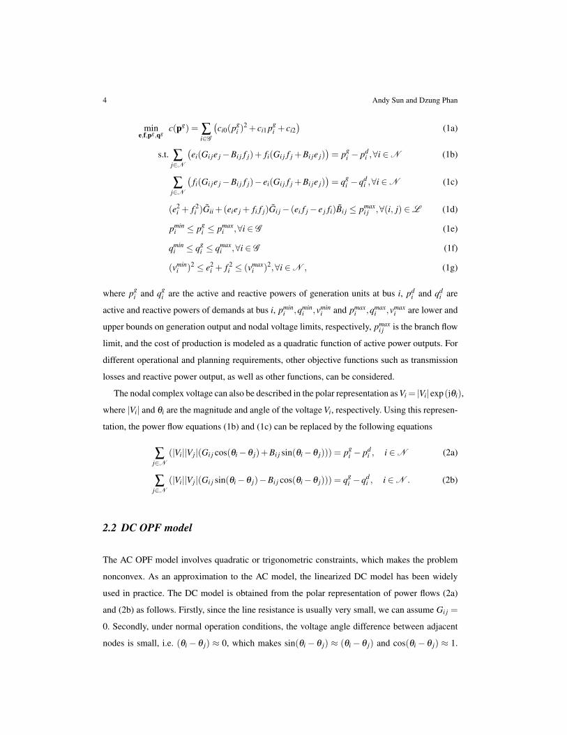
The AC optimal power flow model that minimizes the total production cost can be written as
[15, 19, 38]:
4 Andy Sun and Dzung Phan
mine,f,pg,qg
c(pg) = ∑i∈G
(ci0(pg
i )2 + ci1 pg
i + ci2)
(1a)
s.t. ∑j∈N
(ei(Gi je j−Bi j f j)+ fi(Gi j f j +Bi je j)
)= pg
i − pdi ,∀i ∈N (1b)
∑j∈N
(fi(Gi je j−Bi j f j)− ei(Gi j f j +Bi je j)
)= qg
i −qdi ,∀i ∈N (1c)
(e2i + f 2
i )Gii +(eie j + fi f j)Gi j− (ei f j− e j fi)Bi j ≤ pmaxi j ,∀(i, j) ∈L (1d)
pmini ≤ pg
i ≤ pmaxi ,∀i ∈ G (1e)
qmini ≤ qg
i ≤ qmaxi ,∀i ∈ G (1f)
(vmini )2 ≤ e2
i + f 2i ≤ (vmax
i )2,∀i ∈N , (1g)
where pgi and qg
i are the active and reactive powers of generation units at bus i, pdi and qd
i are
active and reactive powers of demands at bus i, pmini ,qmin
i ,vmini and pmax
i ,qmaxi ,vmax
i are lower and
upper bounds on generation output and nodal voltage limits, respectively, pmaxi j is the branch flow
limit, and the cost of production is modeled as a quadratic function of active power outputs. For
different operational and planning requirements, other objective functions such as transmission
losses and reactive power output, as well as other functions, can be considered.
The nodal complex voltage can also be described in the polar representation as Vi = |Vi|exp(jθi),
where |Vi| and θi are the magnitude and angle of the voltage Vi, respectively. Using this represen-
tation, the power flow equations (1b) and (1c) can be replaced by the following equations
∑j∈N
(|Vi||Vj|(Gi j cos(θi−θ j)+Bi j sin(θi−θ j))) = pgi − pd
i , i ∈N (2a)
∑j∈N
(|Vi||Vj|(Gi j sin(θi−θ j)−Bi j cos(θi−θ j))) = qgi −qd
i , i ∈N . (2b)
2.2 DC OPF model
The AC OPF model involves quadratic or trigonometric constraints, which makes the problem
nonconvex. As an approximation to the AC model, the linearized DC model has been widely
used in practice. The DC model is obtained from the polar representation of power flows (2a)
and (2b) as follows. Firstly, since the line resistance is usually very small, we can assume Gi j =
0. Secondly, under normal operation conditions, the voltage angle difference between adjacent
nodes is small, i.e. (θi− θ j) ≈ 0, which makes sin(θi− θ j) ≈ (θi− θ j) and cos(θi− θ j) ≈ 1.
Electric Power System Operations 5
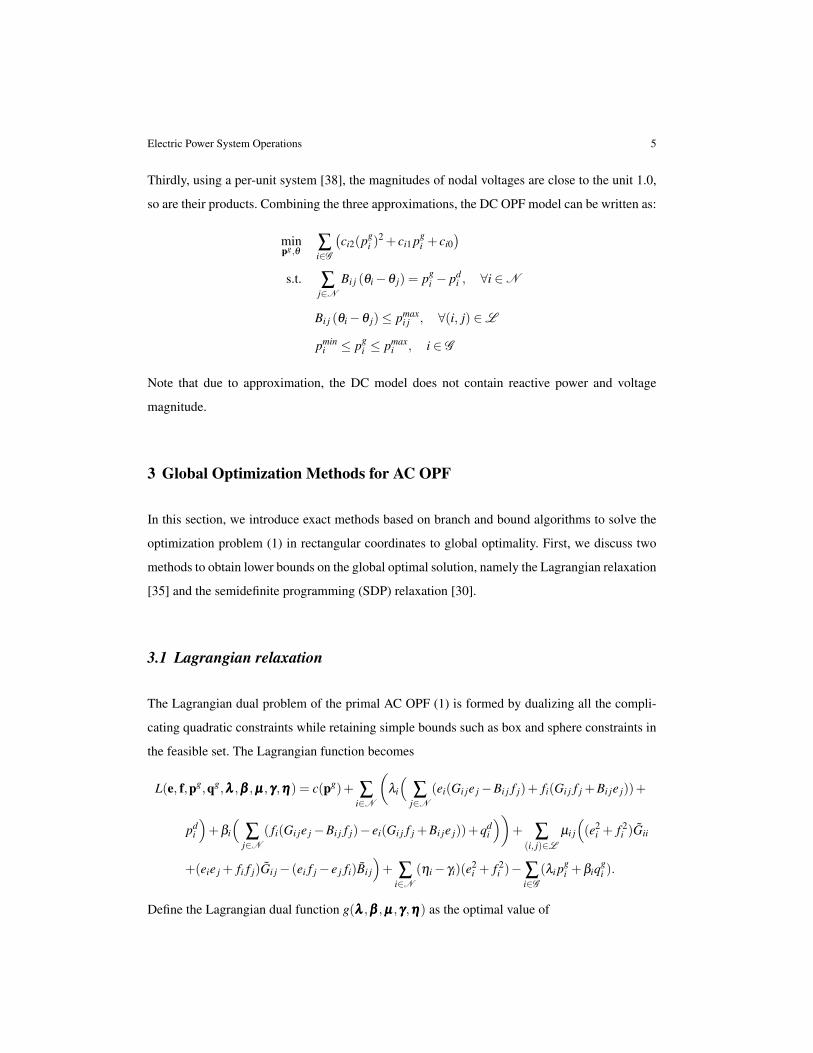
Thirdly, using a per-unit system [38], the magnitudes of nodal voltages are close to the unit 1.0,
so are their products. Combining the three approximations, the DC OPF model can be written as:
minpg,θ
∑i∈G
(ci2(pg
i )2 + ci1 pg
i + ci0)
s.t. ∑j∈N
Bi j (θi−θ j) = pgi − pd
i , ∀i ∈N
Bi j (θi−θ j)≤ pmaxi j , ∀(i, j) ∈L
pmini ≤ pg
i ≤ pmaxi , i ∈ G
Note that due to approximation, the DC model does not contain reactive power and voltage
magnitude.
3 Global Optimization Methods for AC OPF
In this section, we introduce exact methods based on branch and bound algorithms to solve the
optimization problem (1) in rectangular coordinates to global optimality. First, we discuss two
methods to obtain lower bounds on the global optimal solution, namely the Lagrangian relaxation
[35] and the semidefinite programming (SDP) relaxation [30].
3.1 Lagrangian relaxation
The Lagrangian dual problem of the primal AC OPF (1) is formed by dualizing all the compli-
cating quadratic constraints while retaining simple bounds such as box and sphere constraints in
the feasible set. The Lagrangian function becomes
L(e, f,pg,qg,λλλ ,βββ ,µµµ,γγγ,ηηη) = c(pg)+ ∑i∈N
(λi
(∑
j∈N(ei(Gi je j−Bi j f j)+ fi(Gi j f j +Bi je j))+
pdi
)+βi
(∑
j∈N( fi(Gi je j−Bi j f j)− ei(Gi j f j +Bi je j))+qd
i
))+ ∑
(i, j)∈Lµi j
((e2
i + f 2i )Gii
+(eie j + fi f j)Gi j− (ei f j− e j fi)Bi j
)+ ∑
i∈N(ηi− γi)(e2
i + f 2i )−∑
i∈G(λi p
gi +βiq
gi ).
Define the Lagrangian dual function g(λλλ ,βββ ,µµµ,γγγ,ηηη) as the optimal value of
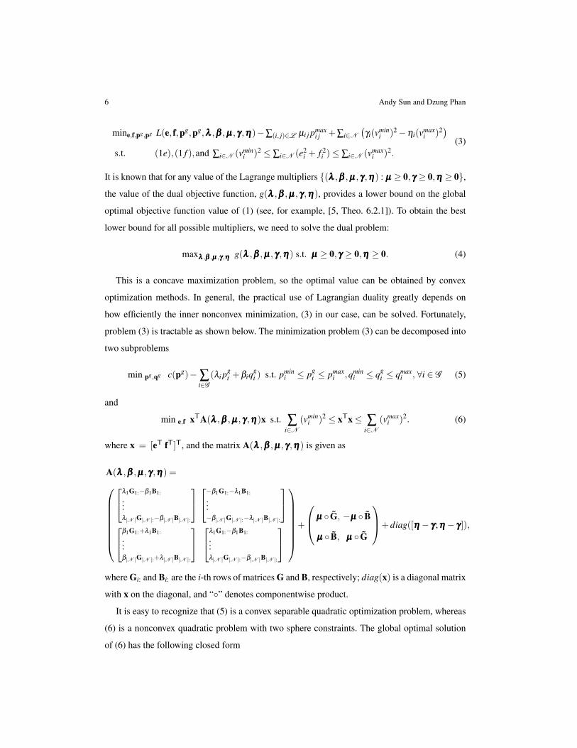
6 Andy Sun and Dzung Phan
mine,f,pg,pg L(e, f,pg,pg,λλλ ,βββ ,µµµ,γγγ,ηηη)−∑(i, j)∈L µi j pmaxi j +∑i∈N
(γi(vmin
i )2−ηi(vmaxi )2
)s.t. (1e),(1 f ),and ∑i∈N (vmin
i )2 ≤ ∑i∈N (e2i + f 2
i )≤ ∑i∈N (vmaxi )2.
(3)
It is known that for any value of the Lagrange multipliers (λλλ ,βββ ,µµµ,γγγ,ηηη) : µµµ ≥ 0,γγγ ≥ 0,ηηη ≥ 0,
the value of the dual objective function, g(λλλ ,βββ ,µµµ,γγγ,ηηη), provides a lower bound on the global
optimal objective function value of (1) (see, for example, [5, Theo. 6.2.1]). To obtain the best
lower bound for all possible multipliers, we need to solve the dual problem:
maxλλλ ,βββ ,µµµ,γγγ,ηηη g(λλλ ,βββ ,µµµ,γγγ,ηηη) s.t. µµµ ≥ 0,γγγ ≥ 0,ηηη ≥ 0. (4)
This is a concave maximization problem, so the optimal value can be obtained by convex
optimization methods. In general, the practical use of Lagrangian duality greatly depends on
how efficiently the inner nonconvex minimization, (3) in our case, can be solved. Fortunately,
problem (3) is tractable as shown below. The minimization problem (3) can be decomposed into
two subproblems
min pg,qg c(pg)−∑i∈G
(λi pgi +βiq
gi ) s.t. pmin
i ≤ pgi ≤ pmax
i ,qmini ≤ qg
i ≤ qmaxi , ∀i ∈ G (5)
and
min e,f xTA(λλλ ,βββ ,µµµ,γγγ,ηηη)x s.t. ∑i∈N
(vmini )2 ≤ xTx≤ ∑
i∈N(vmax
i )2. (6)
where x = [eT fT]T, and the matrix A(λλλ ,βββ ,µµµ,γγγ,ηηη) is given as
A(λλλ ,βββ ,µµµ,γγγ,ηηη) =
λ1G1:−β1B1:...λ|N |G|N |:−β|N |B|N |:
−β1G1:−λ1B1:...−β|N |G|N |:−λ|N |B|N |:
β1G1:+λ1B1:
...β|N |G|N |:+λ|N |B|N |:
λ1G1:−β1B1:...λ|N |G|N |:−β|N |B|N |:
+
µµµ G, −µµµ B
µµµ B, µµµ G
+diag([ηηη− γγγ;ηηη− γγγ]),
where Gi: and Bi: are the i-th rows of matrices G and B, respectively; diag(x) is a diagonal matrix
with x on the diagonal, and “” denotes componentwise product.
It is easy to recognize that (5) is a convex separable quadratic optimization problem, whereas
(6) is a nonconvex quadratic problem with two sphere constraints. The global optimal solution
of (6) has the following closed form
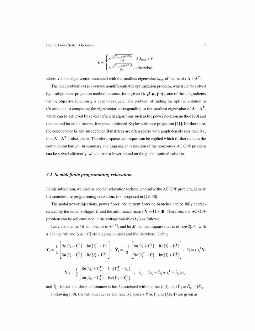
Electric Power System Operations 7
x =
v√
∑i∈N (vmaxi )2
‖v‖ , if λmin < 0
v√
∑i∈N (vmini )2
‖v‖ , otherwise,
where v is the eigenvector associated with the smallest eigenvalue λmin of the matrix A+AT.
The dual problem (4) is a convex nondifferentiable optimization problem, which can be solved
by a subgradient projection method because, for a given (λλλ ,βββ ,µµµ,γγγ,ηηη), one of the subgradients
for the objective function g is easy to evaluate. The problem of finding the optimal solution to
(6) amounts to computing the eigenvector corresponding to the smallest eigenvalue of A+AT,
which can be achieved by several efficient algorithms such as the power iteration method [20] and
the method based on inverse-free preconditioned Krylov subspace projection [21]. Furthermore,
the conductance G and susceptance B matrices are often sparse with graph density less than 0.1,
thus A+AT is also sparse. Therefore, sparse techniques can be applied which further reduces the
computation burden. In summary, the Lagrangian relaxation of the nonconvex AC OPF problem
can be solved efficiently, which gives a lower bound on the global optimal solution.
3.2 Semidefinite programming relaxation
In this subsection, we discuss another relaxation technique to solve the AC OPF problem, namely
the semidefinite programming relaxation, first proposed in [29, 30].
The nodal power injections, power flows, and current flows on branches can be fully charac-
terized by the nodal voltages Vi and the admittance matrix Y = G+ jB. Therefore, the AC OPF
problem can be reformulated in the voltage variables Vi’s as follows.
Let ei denote the i-th unit vector in R|N |, and let Mi denote a square matrix of size 2|N | with
a 1 in the i-th and (i+ |N |)-th diagonal entries and 0’s elsewhere. Define
Yi =12
ReYi +YTi ImYT
i −Yi
ImYi−YTi ReYi +YT
i
, Yi =−12
ImYi +YTi ReYi−YT
i
ReYTi −Yi ImYi +YT
i
, Yi = eieTi Y,
Yi j =12
ReYi j +YTi j ImYT
i j −Yi j
ImYi j−YTi j ReYi j +YT
i j
, Yi j = (Yi j + Yi j)eieTi − Yi jeie
Tj ,
and Yi j denotes the shunt admittance at bus i associated with the line (i, j), and Yi j = Gi j + jBi j.
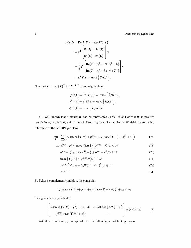
Following [30], the net nodal active and reactive powers Pi(e, f) and Qi(e, f) are given as
8 Andy Sun and Dzung Phan
Pi(e, f) = ReVi I∗i = ReV∗YiV
= xT
ReYi −ImYi
ImYi ReYi
x
=12
xT
ReYi +YTi ImYT
i −Yi
ImYi−YTi ReYi +YT
i
x
= xTYix = trace
YixxT.
Note that x = [ReVT ImVT]T. Similarly, we have
Qi(e, f) = ImVi I∗i = trace
YixxT,
e2i + f 2
i = xTMix = trace
MixxT,
Pi j(e, f) = trace
Yi jxxT.
It is well known that a matrix W can be represented as xxT if and only if W is positive
semidefinite, i.e., W 0, and has rank 1. Dropping the rank condition on W yields the following
relaxation of the AC OPF problem:
minW ∑
i∈G
(ci0(traceYiW+ pd
i )2 + ci1(traceYiW+ pd
i )+ ci2
)(7a)
s.t. pmini − pd
i ≤ traceYiW ≤ pmaxi − pd
i ,∀i ∈N (7b)
qmini −qd
i ≤ trace
YiW≤ qmax
i −qdi ,∀i ∈N (7c)
trace
Yi jW≤ pmax
i j ,∀(i, j) ∈L (7d)
(vmini )2 ≤ traceMiW ≤ (vmax
i )2,∀i ∈N (7e)
W 0. (7f)
By Schur’s complement condition, the constraint
ci0(traceYiW+ pdi )
2 + ci1(traceYiW+ pdi )+ ci2 ≤ αi
for a given αi is equivalent toci1(traceYiW+ pdi )+ ci2−αi
√ci0(traceYiW+ pd
i )
√ci0(traceYiW+ pd
i ) −1
0,∀i ∈ G . (8)
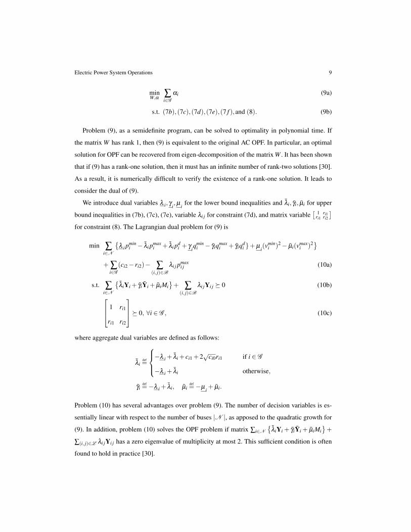
With this equivalence, (7) is equivalent to the following semidefinite program
Electric Power System Operations 9
minW,α
∑i∈G
αi (9a)
s.t. (7b),(7c),(7d),(7e),(7 f ),and (8). (9b)
Problem (9), as a semidefinite program, can be solved to optimality in polynomial time. If
the matrix W has rank 1, then (9) is equivalent to the original AC OPF. In particular, an optimal
solution for OPF can be recovered from eigen-decomposition of the matrix W . It has been shown
that if (9) has a rank-one solution, then it must has an infinite number of rank-two solutions [30].
As a result, it is numerically difficult to verify the existence of a rank-one solution. It leads to
consider the dual of (9).
We introduce dual variables λ i,γ i,µ
ifor the lower bound inequalities and λi, γi, µi for upper
bound inequalities in (7b), (7c), (7e), variable λi j for constraint (7d), and matrix variable[ 1 ri1
ri1 ri2
]for constraint (8). The Lagrangian dual problem for (9) is
min ∑i∈N
λ i p
mini − λi pmax
i + λi pdi + γ
iqmin
i − γiqmaxi + γiqd
i +µi(vmin
i )2− µi(vmaxi )2
+ ∑i∈G
(ci2− ri2)− ∑(i, j)∈B
λi j pmaxi j (10a)
s.t. ∑i∈N
λiYi + γiYi + µiMi
+ ∑
(i, j)∈Bλi jYi j 0 (10b)
1 ri1
ri1 ri2
0, ∀i ∈ G , (10c)
where aggregate dual variables are defined as follows:
λidef=
−λ i + λi + ci1 +2√
ci0ri1 if i ∈ G
−λ i + λi otherwise,
γidef=−λ i + λi, µi
def=−µ
i+ µi.
Problem (10) has several advantages over problem (9). The number of decision variables is es-
sentially linear with respect to the number of buses |N |, as apposed to the quadratic growth for
(9). In addition, problem (10) solves the OPF problem if matrix ∑i∈N
λiYi + γiYi + µiMi+
∑(i, j)∈L λi jYi j has a zero eigenvalue of multiplicity at most 2. This sufficient condition is often
found to hold in practice [30].
10 Andy Sun and Dzung Phan
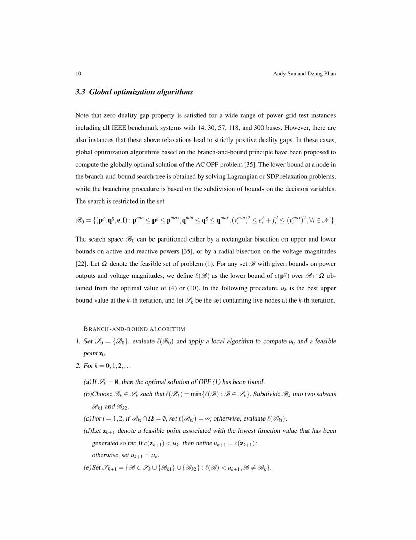
3.3 Global optimization algorithms
Note that zero duality gap property is satisfied for a wide range of power grid test instances
including all IEEE benchmark systems with 14, 30, 57, 118, and 300 buses. However, there are
also instances that these above relaxations lead to strictly positive duality gaps. In these cases,
global optimization algorithms based on the branch-and-bound principle have been proposed to
compute the globally optimal solution of the AC OPF problem [35]. The lower bound at a node in
the branch-and-bound search tree is obtained by solving Lagrangian or SDP relaxation problems,
while the branching procedure is based on the subdivision of bounds on the decision variables.
The search is restricted in the set
B0 = (pg,qg,e, f) : pmin ≤ pg ≤ pmax,qmin ≤ qg ≤ qmax,(vmini )2 ≤ e2
i + f 2i ≤ (vmax
i )2,∀i ∈N .
The search space B0 can be partitioned either by a rectangular bisection on upper and lower
bounds on active and reactive powers [35], or by a radial bisection on the voltage magnitudes
[22]. Let Ω denote the feasible set of problem (1). For any set B with given bounds on power
outputs and voltage magnitudes, we define `(B) as the lower bound of c(pq) over B ∩Ω ob-
tained from the optimal value of (4) or (10). In the following procedure, uk is the best upper
bound value at the k-th iteration, and let Sk be the set containing live nodes at the k-th iteration.
BRANCH-AND-BOUND ALGORITHM
1. Set S0 = B0, evaluate `(B0) and apply a local algorithm to compute u0 and a feasible
point z0.
2. For k = 0,1,2, . . .
(a)If Sk = /0, then the optimal solution of OPF (1) has been found.
(b)Choose Bk ∈Sk such that `(Bk) = min`(B) : B ∈Sk. Subdivide Bk into two subsets
Bk1 and Bk2.
(c)For i = 1,2, if Bki∩Ω = /0, set `(Bki) = ∞; otherwise, evaluate `(Bki).
(d)Let zk+1 denote a feasible point associated with the lowest function value that has been
generated so far. If c(zk+1)< uk, then define uk+1 = c(zk+1);
otherwise, set uk+1 = uk.
(e)Set Sk+1 = B ∈Sk ∪Bk1∪Bk2 : `(B)< uk+1,B 6= Bk.
Electric Power System Operations 11
Because the diameter of Bk tends to zero as k tends to infinity, the bounding scheme is con-
sistent. In addition, because of the selection of the live node in Step 2b, the smallest lower bound
is increasing, thus the algorithm is convergent [24].
4 Security-Constrained Optimal Power Flow
Contingency analysis is routinely performed in the economic dispatch practice. The goal is to
ensure that demand can be satisfied in the normal case and in the case of contingencies, where
any one or more components in the power system, such as generators, transmission lines, trans-
formers, or other equipments, experience unexpected failure. The OPF problem with contingency
constraints is often referred to as the Security-Constrained OPF (SCOPF). There are two major
types of SCOPF models: the preventive model [2] and the corrective model [33].
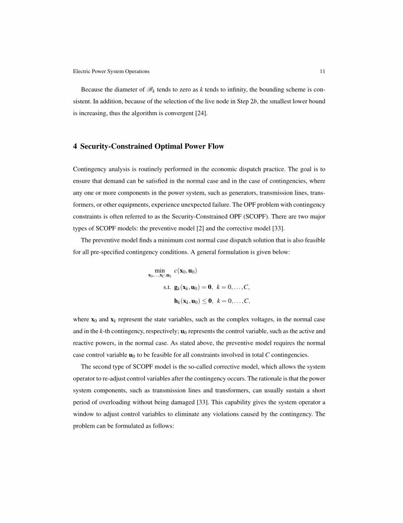
The preventive model finds a minimum cost normal case dispatch solution that is also feasible
for all pre-specified contingency conditions. A general formulation is given below:
minx0,...,xC ,u0
c(x0,u0)
s.t. gk(xk,u0) = 0, k = 0, . . . ,C,
hk(xk,u0)≤ 0, k = 0, . . . ,C,
where x0 and xk represent the state variables, such as the complex voltages, in the normal case
and in the k-th contingency, respectively; u0 represents the control variable, such as the active and
reactive powers, in the normal case. As stated above, the preventive model requires the normal
case control variable u0 to be feasible for all constraints involved in total C contingencies.
The second type of SCOPF model is the so-called corrective model, which allows the system
operator to re-adjust control variables after the contingency occurs. The rationale is that the power
system components, such as transmission lines and transformers, can usually sustain a short
period of overloading without being damaged [33]. This capability gives the system operator a
window to adjust control variables to eliminate any violations caused by the contingency. The
problem can be formulated as follows:
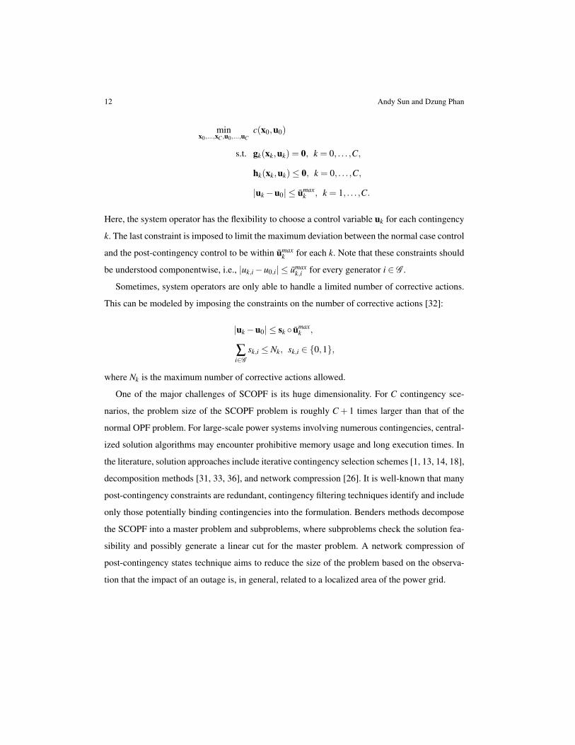
12 Andy Sun and Dzung Phan
minx0,...,xC ,u0,...,uC
c(x0,u0)
s.t. gk(xk,uk) = 0, k = 0, . . . ,C,
hk(xk,uk)≤ 0, k = 0, . . . ,C,
|uk−u0| ≤ umaxk , k = 1, . . . ,C.
Here, the system operator has the flexibility to choose a control variable uk for each contingency
k. The last constraint is imposed to limit the maximum deviation between the normal case control
and the post-contingency control to be within umaxk for each k. Note that these constraints should
be understood componentwise, i.e., |uk,i−u0,i| ≤ umaxk,i for every generator i ∈ G .
Sometimes, system operators are only able to handle a limited number of corrective actions.
This can be modeled by imposing the constraints on the number of corrective actions [32]:
|uk−u0| ≤ sk umaxk ,
∑i∈G
sk,i ≤ Nk, sk,i ∈ 0,1,
where Nk is the maximum number of corrective actions allowed.
One of the major challenges of SCOPF is its huge dimensionality. For C contingency sce-
narios, the problem size of the SCOPF problem is roughly C + 1 times larger than that of the
normal OPF problem. For large-scale power systems involving numerous contingencies, central-
ized solution algorithms may encounter prohibitive memory usage and long execution times. In
the literature, solution approaches include iterative contingency selection schemes [1, 13, 14, 18],
decomposition methods [31, 33, 36], and network compression [26]. It is well-known that many
post-contingency constraints are redundant, contingency filtering techniques identify and include
only those potentially binding contingencies into the formulation. Benders methods decompose
the SCOPF into a master problem and subproblems, where subproblems check the solution fea-
sibility and possibly generate a linear cut for the master problem. A network compression of
post-contingency states technique aims to reduce the size of the problem based on the observa-
tion that the impact of an outage is, in general, related to a localized area of the power grid.
Electric Power System Operations 13
5 Distributed Algorithms for AC OPF
Previous sections introduce models and solution methods for AC OPF problems, which require
a central control entity gathering system wide information and implementing the solution algo-
rithms. However, in some situations, decentralized decision making is more appealing or even
necessary. For instance, in a large interconnected power system involving multiple Independent
System Operators (ISO) or utilities, information pooling and sharing may be limited by institu-
tional arrangements. The central controller in this case has no access to detailed information to
implement the centralized optimization algorithms. To achieve the system wide optimal dispatch
decision, a decentralized algorithm is needed, where subsystems solve localized problems and
exchange limited amount of information with neighboring subsystems. A distributed algorithm
is also appealing from reliability perspective. In the event of power system disruption such as
communication failure between regions, centralized control would be disrupted, while a decen-
tralized scheme can handle the situation in a more flexible way.
Baldick and his colleagues in a series of papers first demonstrated the viability of distributed
algorithms for optimal power flow problems [27, 4, 28]. Since then, several papers have con-
tributed to the topic. In the following, we categorize existing approaches based on the type of
OPF models, decomposition methods, and algorithmic frameworks.
1. OPF models: Both AC and DC OPF problems have been studied. In particular, [27, 4, 28, 17,
34, 11] have proposed distributed algorithms for AC OPF problems, while [16, 3, 10, 12] have
proposed for DC OPF problems. In [16], the authors use a nonlinear DC model to account for
network losses. Distributed algorithms for security-constrained DC OPF problem have also
been proposed [12].
2. Decomposition methods: A large power system is usually divided to sub-control regions,
such as ISOs and utilities, interconnected by tie-lines. The coupling between subsystems
arises from constraints such as power flow balance equations and thermal limits on trans-
mission lines. In order to apply a distributed algorithm, the coupling between subsystems
need to be broken down. A common idea behind all the decomposition methods proposed
in the literature is to introduce redundant variables in the overlapping regions between sub-
systems. These redundant variables can be power injections and voltages on fictitious buses
introduced on tie-lines [27, 4, 28, 16, 17, 34]; or, redundant power flow variables on tie-lines
[3, 10, 12, 11].
14 Andy Sun and Dzung Phan
3. Algorithmic framework: After redundant variables are introduced, the centralized OPF
model is decomposed into subproblems. A common approach is to relax coupling constraints
using Lagrangian relaxation or some of its variants. In particular, the existing proposals can
be divided into two groups. The first group uses the exact framework of Lagrangian or aug-
mented Lagrangian relaxation, where the coupling constraints are relaxed by introducing La-
grange multipliers, the resulting Lagrangian problem is solved by a distributed algorithm, and
the Lagrange multipliers (the shadow prices) are updated by a subgradient scheme. For exam-
ple, the auxiliary problem principle (APP) is used to solve the Lagrangian problem in [27, 4].
The alternating direction method and the predictor-corrector proximal method are applied and
compared to the APP method in [28]. These three methods have comparable performance in
terms of number of iterations and computation time. The other group of methods uses a variant
of Lagrangian relaxation framework, where the KKT system of the subproblem is solved ap-
proximately in each iteration [17, 34, 3, 10, 12]. The key observation is that stacking together
the KKT conditions of subsystems gives the KKT condition of the entire system. Therefore,
when the distributed algorithm converges, the solution satisfies the overall KKT condition and
thus is at least a stationary point of the centralized problem. It is worth mentioning that the
distributed algorithm frameworks such as the auxiliary problem principle or the alternating di-
rection methods are originally proposed for convex optimization problems. The convergence
is not guaranteed for general non-convex problems like the AC OPF problems.
6 Security-Constrained Unit Commitment Problem
In a centralized control system, the system operator has access to a wide range of detailed eco-
nomic and operational data, including production costs and physical constraints of the generation
units, system load forecast, system reserve requirement, and network parameters. Based on these
data, the system operator need to decide a commitment schedule of generation units for the next
24 hours or a longer period of time, under which the forecast demand can be met with the least
total commitment and dispatch cost, and very importantly, the security constraints induced by the
N−1 criterion are satisfied. Therefore, the unit commitment model used in the current practice
is a deterministic scheduling model with many complicating constraints.
It is also important that the system operator accounts for uncertainties in the load forecast and
unexpected outages of generators and transmission lines when making the unit commitment de-
Electric Power System Operations 15
cision. The traditional and still widely used approach is to reserve a certain amount of generation
resources for the purpose of fast response to emergencies such as loss of generators and trans-
mission lines or sudden load peak. This amount of stand-by capacity is called reserves, which
are further classified into different categories based on the speed of response, such as ten-minute
spinning reserve (TMSR), ten-minute nonspinning reserve (TMNSR), and thirty-minute oper-
ating reserve (TMOR). Other types of reserves exist. For example, regulation reserves are the
generation capacity controlled by automatic systems that respond to frequency changes in the
power system every few seconds.
The unit commitment model then includes decision variables for the amount of reserves pro-
vided by each generator, and also includes constraints that the total reserves in the power system
should meet certain reserve requirements. Such reserve requirements are usually pre-determined
by the system operator as a part of the operating rules. In the following, the security-constrained
unit commitment model is presented.
The decision variables are: binary variables xti ,u
ti,v
ti for commitment decisions and continuous
variables pti and qt
i,a for generation and reserve decisions, where xti = 1 if generator i is producing
electricity, i.e. in the on state, at time t, and xti = 0 otherwise; ut
i = 1 if generator i is turned on from
the off state at time t; vti = 1 if generator i is turned off at time t; pt
i is the amount of electricity
produced by generator i at time t; and qti,a is the amount of reserve provided by generator i for
reserve type a at time t.
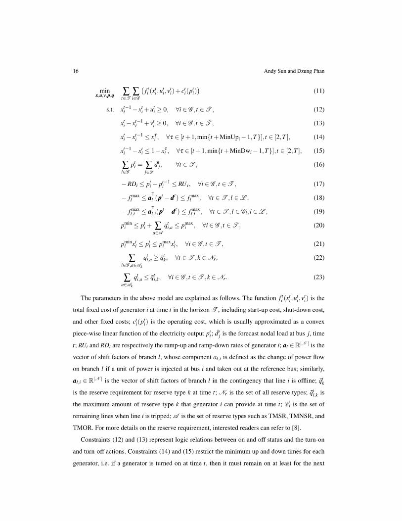
The basic optimization model is given as below [23, 37]:
16 Andy Sun and Dzung Phan
minxxx,uuu,vvv,ppp,qqq ∑
t∈T∑i∈G
(f ti (x
ti ,u
ti,v
ti)+ ct
i(pti))
(11)
s.t. xt−1i − xt
i +uti ≥ 0, ∀i ∈ G , t ∈T , (12)
xti− xt−1
i + vti ≥ 0, ∀i ∈ G , t ∈T , (13)
xti− xt−1
i ≤ xτi , ∀τ ∈ [t +1,mint +MinUpi−1,T], t ∈ [2,T ], (14)
xt−1i − xt
i ≤ 1− xτi , ∀τ ∈ [t +1,mint +MinDwi−1,T], t ∈ [2,T ], (15)
∑i∈G
pti = ∑
j∈Ddt
j, ∀t ∈T , (16)
−RDi ≤ pti− pt−1
i ≤ RU i, ∀i ∈ G , t ∈T , (17)
− f maxl ≤ aaa
T
l (pppt −dddt)≤ f maxl , ∀t ∈T , l ∈L , (18)
− f maxl,i ≤ aaa
T
l,i(pppt −dddt)≤ f maxl,i , ∀t ∈T , l ∈ Ci, i ∈L , (19)
pmini ≤ pt
i + ∑a∈A
qti,a ≤ pmax
i , ∀i ∈ G , t ∈T , (20)
pmini xt
i ≤ pti ≤ pmax
i xti , ∀i ∈ G , t ∈T , (21)
∑i∈G ,a∈Ak
qti,a ≥ qt
k, ∀t ∈T ,k ∈Nr, (22)
∑a∈Ak
qti,a ≤ qt
i,k, ∀i ∈ G , t ∈T ,k ∈Nr. (23)
The parameters in the above model are explained as follows. The function f ti (x
ti ,u
ti,v
ti) is the
total fixed cost of generator i at time t in the horizon T , including start-up cost, shut-down cost,
and other fixed costs; cti(pt
i) is the operating cost, which is usually approximated as a convex
piece-wise linear function of the electricity output pti; dt
j is the forecast nodal load at bus j, time
t; RUi and RDi are respectively the ramp-up and ramp-down rates of generator i; aaal ∈R|N | is the
vector of shift factors of branch l, whose component al,i is defined as the change of power flow
on branch l if a unit of power is injected at bus i and taken out at the reference bus; similarly,
aaal,i ∈ R|N | is the vector of shift factors of branch l in the contingency that line i is offline; qtk
is the reserve requirement for reserve type k at time t; Nr is the set of all reserve types; qti,k is
the maximum amount of reserve type k that generator i can provide at time t; Ci is the set of
remaining lines when line i is tripped; A is the set of reserve types such as TMSR, TMNSR, and
TMOR. For more details on the reserve requirement, interested readers can refer to [8].
Constraints (12) and (13) represent logic relations between on and off status and the turn-on
and turn-off actions. Constraints (14) and (15) restrict the minimum up and down times for each
generator, i.e. if a generator is turned on at time t, then it must remain on at least for the next
Electric Power System Operations 17
(MinUpi−1) periods, and similar for the shutdown constraint. Constraint (16) is the energy bal-
ance for each time period. Constraint (17) is the ramping constraint, which couples consecutive
time periods. Constraint (18) is the linearized power flow equations using shift factors for the
base case, where all transmission lines are functioning. Constraint (19) is the power flow limits
under the i-th contingency. Constraint (20) limits the total production and reserve for each gener-
ator. Constraint (21) limits the production level of each generator. Constraint (22) is the system
reserve requirement for reserve category k at time t. Constraint (23) provides an upper bound on
generator i’s reserve capacity.
7 Adaptive Robust Optimization for SCUC under Uncertainty
The rapid growth of renewable energy resources such as wind and solar power leads to signif-
icantly increased uncertainty in both supply and demand in the power systems. The traditional
deterministic approach introduced in the previous section is challenged in both its economic ef-
ficiency and operational effectiveness. In this section, we introduce recent developments in unit
commitment models using the methodology of adaptive robust optimization [6, 7, 9].
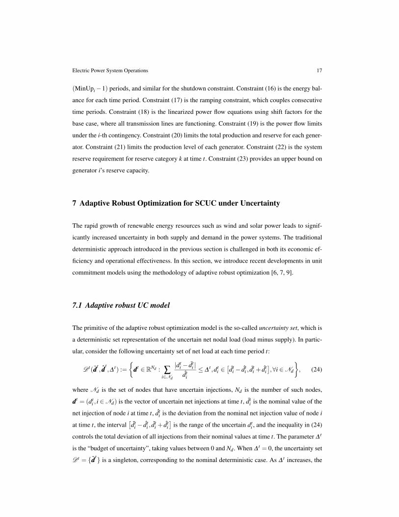
7.1 Adaptive robust UC model
The primitive of the adaptive robust optimization model is the so-called uncertainty set, which is
a deterministic set representation of the uncertain net nodal load (load minus supply). In partic-
ular, consider the following uncertainty set of net load at each time period t:
D t(dddt, ddd
t,∆ t) :=
dddt ∈ RNd : ∑
i∈Nd
|dti − dt
i |dt
i≤ ∆
t ,dti ∈[dt
i − dti , d
ti + dt
i],∀i ∈Nd
, (24)
where Nd is the set of nodes that have uncertain injections, Nd is the number of such nodes,
dddt = (dti , i ∈Nd) is the vector of uncertain net injections at time t, dt
i is the nominal value of the
net injection of node i at time t, dti is the deviation from the nominal net injection value of node i
at time t, the interval[dt
i − dti , d
ti + dt
i]
is the range of the uncertain dti , and the inequality in (24)
controls the total deviation of all injections from their nominal values at time t. The parameter ∆ t
is the “budget of uncertainty”, taking values between 0 and Nd . When ∆ t = 0, the uncertainty set
D t = dddt is a singleton, corresponding to the nominal deterministic case. As ∆ t increases, the
18 Andy Sun and Dzung Phan
size of the uncertainty set D t enlarges. This means that larger total deviation from the expected
net injection is considered, so that the resulting robust UC solutions are more conservative and
the system is protected against a higher degree of uncertainty. When ∆ t = Nd , D t equals to the
entire hypercube defined by the intervals for each dti for i ∈Nd .
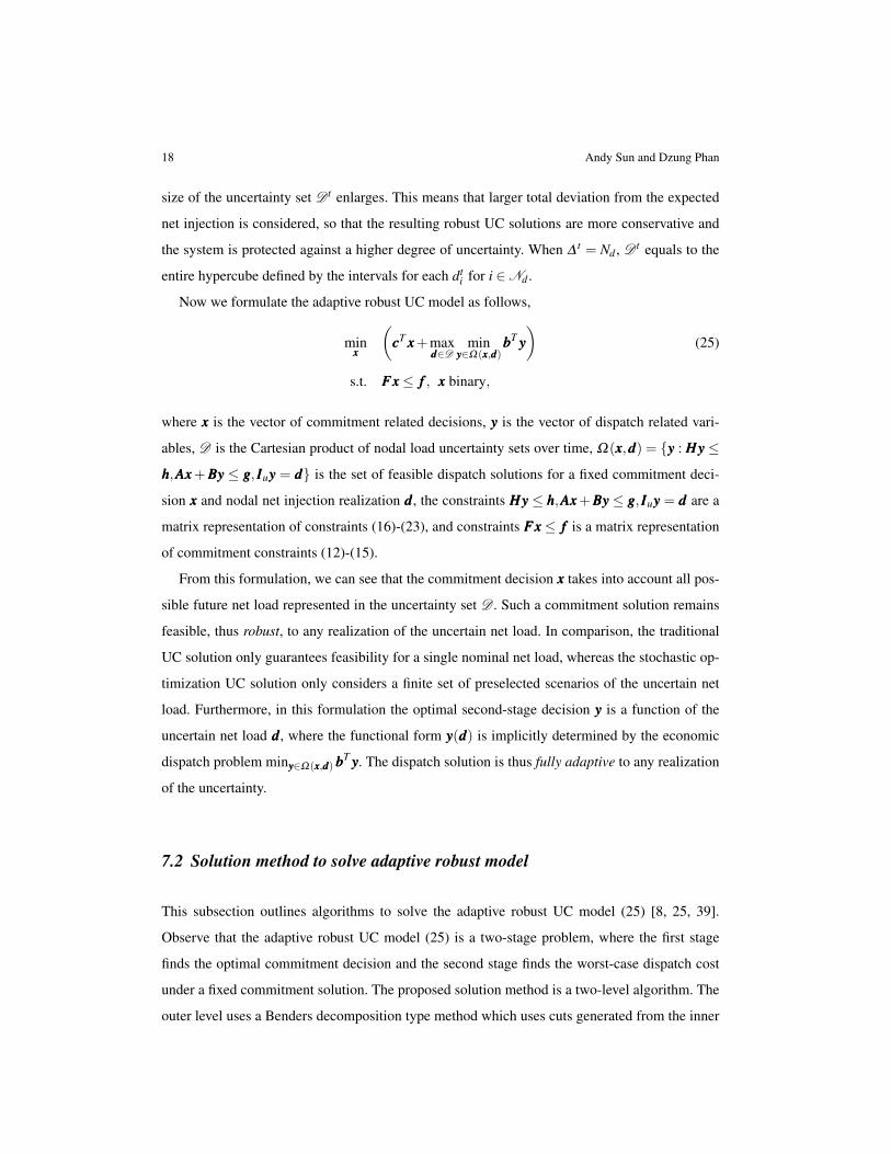
Now we formulate the adaptive robust UC model as follows,
minxxx
(cccT xxx+max
ddd∈Dmin
yyy∈Ω(xxx,ddd)bbbT yyy
)(25)
s.t. FFFxxx≤ fff , xxx binary,
where xxx is the vector of commitment related decisions, yyy is the vector of dispatch related vari-
ables, D is the Cartesian product of nodal load uncertainty sets over time, Ω(xxx,ddd) = yyy : HHHyyy ≤
hhh,AAAxxx+BBByyy ≤ ggg, IIIuyyy = ddd is the set of feasible dispatch solutions for a fixed commitment deci-
sion xxx and nodal net injection realization ddd, the constraints HHHyyy ≤ hhh,AAAxxx+BBByyy ≤ ggg, IIIuyyy = ddd are a
matrix representation of constraints (16)-(23), and constraints FFFxxx≤ fff is a matrix representation
of commitment constraints (12)-(15).
From this formulation, we can see that the commitment decision xxx takes into account all pos-
sible future net load represented in the uncertainty set D . Such a commitment solution remains
feasible, thus robust, to any realization of the uncertain net load. In comparison, the traditional
UC solution only guarantees feasibility for a single nominal net load, whereas the stochastic op-
timization UC solution only considers a finite set of preselected scenarios of the uncertain net
load. Furthermore, in this formulation the optimal second-stage decision yyy is a function of the
uncertain net load ddd, where the functional form yyy(ddd) is implicitly determined by the economic
dispatch problem minyyy∈Ω(xxx,ddd) bbbT yyy. The dispatch solution is thus fully adaptive to any realization
of the uncertainty.
7.2 Solution method to solve adaptive robust model
This subsection outlines algorithms to solve the adaptive robust UC model (25) [8, 25, 39].
Observe that the adaptive robust UC model (25) is a two-stage problem, where the first stage
finds the optimal commitment decision and the second stage finds the worst-case dispatch cost
under a fixed commitment solution. The proposed solution method is a two-level algorithm. The
outer level uses a Benders decomposition type method which uses cuts generated from the inner
Electric Power System Operations 19
level algorithm. The inner level solves the second-stage problem maxddd∈D minyyy∈Ω(xxx,ddd) bbbT yyy, which
can be reformulated either as a bilinear optimization problem by dualizing the inner dispatch
problem minyyy∈Ω(xxx,ddd) bbbT yyy [8], or as a mixed-integer linear optimization problem by introducing
binary variables and big-M constants to linearize the bilinear terms [25, 39]. In [8], the bilinear
optimization problem is solved by an outer approximation algorithm. In [25, 39], the MILP
problem is solved by commercial MIP solvers. The overall framework of the two-level algorithm
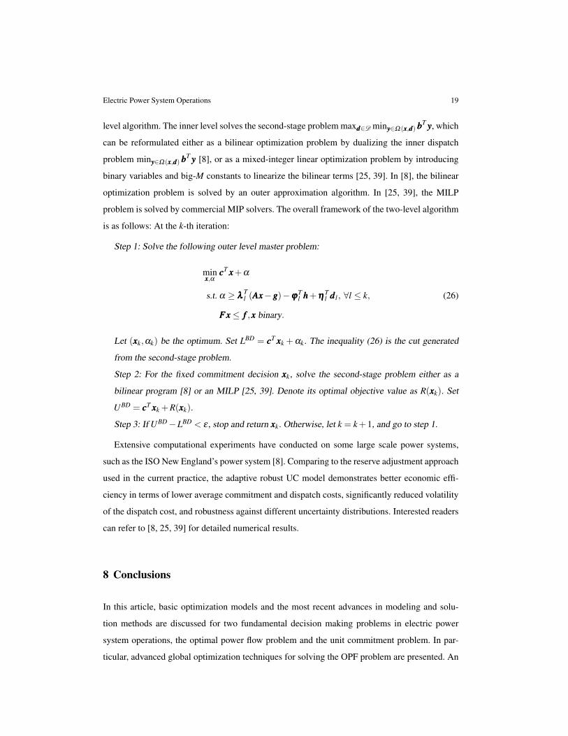
is as follows: At the k-th iteration:
Step 1: Solve the following outer level master problem:
minxxx,α
cccT xxx+α
s.t. α ≥ λλλTl (AAAxxx−ggg)−ϕϕϕ
Tl hhh+ηηη
Tl dddl , ∀l ≤ k, (26)
FFFxxx≤ fff ,xxx binary.
Let (xxxk,αk) be the optimum. Set LBD = cccT xxxk +αk. The inequality (26) is the cut generated
from the second-stage problem.
Step 2: For the fixed commitment decision xxxk, solve the second-stage problem either as a
bilinear program [8] or an MILP [25, 39]. Denote its optimal objective value as R(xxxk). Set
UBD = cccT xxxk +R(xxxk).
Step 3: If UBD−LBD < ε , stop and return xxxk. Otherwise, let k = k+1, and go to step 1.
Extensive computational experiments have conducted on some large scale power systems,
such as the ISO New England’s power system [8]. Comparing to the reserve adjustment approach
used in the current practice, the adaptive robust UC model demonstrates better economic effi-
ciency in terms of lower average commitment and dispatch costs, significantly reduced volatility
of the dispatch cost, and robustness against different uncertainty distributions. Interested readers
can refer to [8, 25, 39] for detailed numerical results.
8 Conclusions
In this article, basic optimization models and the most recent advances in modeling and solu-
tion methods are discussed for two fundamental decision making problems in electric power
system operations, the optimal power flow problem and the unit commitment problem. In par-
ticular, advanced global optimization techniques for solving the OPF problem are presented. An
20 Andy Sun and Dzung Phan
adaptive robust optimization model and solution methods for the unit commitment problem are
introduced, which provide a new, effective framework for power system operations under uncer-
tainty. We have also discussed contingency analysis for large-scale power systems, as well as
distributed optimization schemes for decentralized control of the power systems. In conclusion,
modern optimization methods play a central role in power system operations. Further advances
are needed to meet new challenges arising in the fast evolving modern power systems.
References
1. Alsac, O., Bright, J., Prais, M., Stott, B.: Further developments in LP-based optimal power flow. IEEE Trans.
Power Syst. 5(3), 697–711 (1990)
2. Alsac, O., Stott, B.: Optimal load flow with steady state security. IEEE Trans. Power Appa. Syst. PAS-93(3),
745–751 (1974)
3. Bakirtzis, A.G., Biskas, P.N.: A decentralized solution to the dc-opf of interconnected power systems. IEEE
Trans. Power Syst. 18(3), 1007–1013 (2003)
4. Baldick, R., Kim, B.H., Chase, C., Luo, Y.: A fast distributed implementation of optimal power flow. IEEE
Trans. Power Syst. 14(3), 858–864 (1999)
5. Bazarra, M.S., Sherali, H.D., Shetty, C.M.: Nonlinear Programming: Theory and Algorithms, 3rd edn. John
Wiley and Sons, Hoboken, NJ (2006)
6. Ben-Tal, A., Ghaoui, L.E., Nemirovski, A.: Robust Optimization. Princeton Series in Applied Mathematics.
Princeton University Press (2009)
7. Ben-Tal, A., Goryashko, A., E., G., Nemirovski, A.: Adjustable robust solutions of uncertain linear programs.
Math. Program. 99(2), 351–376 (2004)
8. Bertsimas, D., Litvinov, E., Sun, X.A., Zhao, J., Zheng, T.: Adaptive robust optimization for the security
constrained unit commitment problem. IEEE Trans. Power Syst. (2012). To appear.
9. Bertsimas, D., Sim, M.: The price of robustness. Operations Research 52, 35–53 (2004)
10. Biskas, P.N., Bakirtzis, A.G.: Decentralized security constrained dc-opf of interconnected power systems.
IEE Proc.-Gener. Transm. Distrib. 151(6), 747–754 (2004)
11. Biskas, P.N., Bakirtzis, A.G.: Decentralized opf of large multiarea power systems. IEE Proc.-Gener. Transm.
Distrib. 153(1), 99–105 (2006)
12. Biskas, P.N., Bakirtzis, A.G., Macheras, N.I., Pasialis, N.K.: A decentralized implementation of dc optimal
power flow on a network of computers. IEEE Trans. Power Syst. 20(1), 25–33 (2005)
13. Bouffard, F., Galiana, F.D., Arroyo, J.M.: Umbrella contingencies in security constrained optimal power flow.
In: 15th Power Systems Computation Conference (PSCC 05). Liege, Belgium (2005)
14. Capitanescu, F., Glavic, M., Ernst, D., Wehenkel, L.: Contingency filtering techniques for preventive security-
constrained optimal power flow. IEEE Trans. Power Syst. 22(4), 1690–1697 (2007)
Electric Power System Operations 21
15. Carpentier, J.: Contribution to the economic dispatch problem. Bulletin Society Francaise Electriciens 8(3),
431–447 (1962)
16. Conejo, A.J., Aguado, J.A.: Multi-area coordinated decentralized dc optimal power flow. IEEE Trans. Power
Syst. 13(4), 1272–1278 (1998)
17. Conejo, A.J., Nogales, F.J., Prieto, F.J.: A decomposition procedure based on approximate newton directions.
Math. Program. 93, 495–515 (2002)
18. Ernst, D., Ruiz-Vega, D., Pavella, M., Hirsch, P.M., Sobajic, D.: A unified approach to transient stability
contingency filtering, ranking and assessment. IEEE Trans. Power Syst. 16(3), 435–443 (2001)
19. Glover, J.D., Sarma, M.S., Overbye, T.J.: Power Systems Analysis and Design. Thomson Learning, Toronto
(2008)
20. Golub, G.H., van Loan, C.F.: Matrix Computations, second edn. The Johns Hopkins University Press, Balti-
more, MD and London, UK (1990)
21. Golub, G.H., Ye, Q.: An inverse free preconditioned Krylov subspace method for symmetric generalized
eigenvalue problems. SIAM J. Sci. Comput. 24(1), 312–334 (2002)
22. Gopalakrishnan, A., Raghunathan, A., Nikovski, D., Biegler, .L.: Global optimization of optimal power flow
using a branch and bound algorithm. In: 50th Annual Allerton Conference on Communication, Control and
Computing. Urbana-Champaign, IL (2012)
23. Guan, X., Luh, P.B., Amalfi, J.A.: An optimization-based method for unit commitment. International Journal
of Electrical Power and Energy Systems 14, 9–17 (1996)
24. Horst, R., Hoang, T.: Global Optimization: Deterministic Approaches. Springer-Verlag (1996)
25. Jiang, R., Wang, J., Guan, Y.: Robust unit commitment with wind power and pumped storage hydro. IEEE
Trans. Power Syst. 27(2), 800–810 (2012)
26. Karoui, K., Crisciu, H., Szekut, A., Stubbe, M.: Large scale security constrained optimal power flow. In: 16th
Power System Computation Conference. Glasgow, Scotland (2008)
27. Kim, B.H., Baldick, R.: Coarse-grained distributed optimal power flow. IEEE Trans. Power Syst. 12(2),
932–939 (1997)
28. Kim, B.H., Baldick, R.: A comparison of distributed optimal power flow algorithms. IEEE Trans. Power
Syst. 15(2), 599–604 (2000)
29. Lavaei, J., Low, S.: Convexification of optimal power flow problem. In: Forty-Eighth Annual Allerton Con-
ference on Communication, Control and Computing. Monticello, IL (2010)
30. Lavaei, J., Low, S.: Zero duality gap in optimal power flow problem. IEEE Trans. Power Syst. 27(1), 92–107
(2012)
31. Li, Y., McCalley, J.D.: Decomposed SCOPF for improving effciency. IEEE Trans. Power Syst. 24(1), 494–
495 (2009)
32. Marano-Marcolini, A., Capitanescu, F., Martinez-Ramos, J., Wehenkel, L.: Exploiting the use of dc scopf
approximation to improve iterative ac scopf algorithms. IEEE Trans. Power Syst. 27(3), 1459 –1466 (2012)
33. Monticelli, A., Pereira, M.V.F., Granville, S.: Security-constrained optimal power flow with post-contingency
corrective rescheduling. IEEE Trans. Power Syst. 2(1), 175–180 (1987)
34. Nogales, F.J., Prieto, F.J., Conejo, A.J.: A decomposition methodology applied to the multi-area optimal
power flow problem. Annals of Operations Research 120, 99–116 (2003)
22 Andy Sun and Dzung Phan
35. Phan, D.T.: Lagrangian duality and branch-and-bound algorithms for optimal power flow. Operations Re-
search 60(2), 275–285 (2012)
36. Phan, D.T., Kalagnanam, J.: Distributed methods for solving the security-constrained optimal power flow
problem. In: Proceedings of the 2012 IEEE PES Innovative Smart Grid Technologies (ISGT), pp. 1–7 (2012)
37. Wang, S., Shahidehpour, S., Kirschen, D., Mokhtari, S., Irisarri, G.: Short-term generation scheduling with
transmission constraints using augmented lagrangian relaxation. IEEE Trans. Power Syst. 10, 1294–1301
(1995)
38. Wood, A.J., Wollenberg, B.F.: Power Generation Operation and Control. John Wiley & Sons, Inc., New York
(1996)
39. Zhao, L., Zeng, B.: Robust unit commitment problem with demand response and wind energy. Technical
Report University of South Florida