N 7 a - 1 9 46 5

NASA CR-120967

MODERN METHODOLOGY OF DESIGNING TARGET RELIABILITY

INTO ROTATING MECHANICAL COMPONENTS

by Dimitri B. Kececioglu and Louie B. Chester

THE UNIVERSITY OF ARIZONACollege of Engineering

Engineering Experiment Station

F I L ECOPY

Prepared for

NATIONAL AERONAUTICS AND SPACE ADMINISTRATION

NASA Lewis Research CenterGrant NCR 03-002-044

1. Report No.

NASA CR-1209672. Government Accession No. 3. Recipient's Catalog No.

4. Title and Subtitle

MODERN METHODOLOGY OF DESIGNING TARGETRELIABILITY INTO ROTATING MECHANICAL COMPONENTS

5. Report Date

January 31, 1973

6. Performing Organization Code

7. Author(s)

Dimitri B. Kececioglu and Louie B. Chester

8. Performing Organization Report No.

10. Work Unit No.

9. Performing Organization Name and Address

The University of ArizonaTucson, Arizona 85721

11. Contract or Grant No.

NCR 03-022-044

12. Sponsoring Agency Name and Address

National Aeronautics and Space AdministrationWashington, D.C. 20546

13. Type of Report and Period Covered

Contractor Report14. Sponsoring Agency Code

15. Supplementary Notes

Project Manager, Vincent R. Lalli, Spacecraft Technology Division, NASA Lewis ResearchCenter, Cleveland, Ohio

16. Abstract

Theoretical research done for the development of a methodology for designing specified

reliabilities into rotating mechanical components is referenced to prior reports submitted

to NASA on this research. Experimentally determined distributional cycles-to-failure

versus maximum alternating nominal strength (S-N) diagrams, and distributional mean

nominal strength versus maximum alternating nominal strength (Goodman) diagrams are

presented. These distributional S-N and Goodman diagrams are for AISI 4340 steel, R 35/4'

hardness, round, cylindrical specimens 0.735 in. in diameter and 6 in. long with a

circumferential groove 0.145 in. radius for a theoretical stress concentration K = 1.42

for Phase I research and 0.034 in. radius for a K =2.34 for Phase II research. The

specimens are subjected to reversed bending and steady torque in specially built, three

complex-fatigue research machines. Based on these results,the effects on the distributional

S-N and Goodman diagrams and on service life of superimposing steady torque on reversed

bending are established, as well as the effect of various stress concentrations. In

addition a computer program for determining the three-parameter Weibull distribution

representing the cycles-to-failure data, and two methods for calculating the reliability

of components subjected to cumulative fatigue loads are given.

17. Key Words (Suggested by Author(s))

Mechanical Reliability Distributional S-N

Design by Reliability Diagrams

Probabilistic Design Distributional GoodmanDiagram

Cycles-to-Failure Distributions

18. Distribution Statement

Unclassified - unlimited

19. Security Classif. (of this report)

Unclassified20. Security Classif. (of this page)

Unclassified21. No. of Pages

xiii + 183

22. Price*

' For sale by the National Technical Information Service, Springfield, Virginia 22151ii

NASA CR - 120967

FINAL REPORT

MODERN METHODOLOGY OF DESIGNING TARGET

RELIABILITY INTO ROTATING MECHANICAL COMPONENTS

by Dimitri B. Kececioglu and Louie B. Chester

THE UNIVERSITY OF ARIZONA

College of Engineering

Engineering Experiment Station

prepared for

NATIONAL AERONAUTICS AND SPACE ADMINISTRATION

NASA Lewis Research Center

Grant NCR 03-002-044

111

TABLE OF CONTENTS

Page

TITLE PAGE iii

LIST OF FIGURES vi

LIST OF TABLES x

SUMMARY xiii

1. INTRODUCTION 1

1.1 BACKGROUND 1

1.2 EXPERIMENTAL RESEARCH OPERATION 3

2. EXPERIMENTAL RESEARCH 7

2.1 PHASE I RESEARCH COMPLETION 7

2.2 PHASE II RESEARCH 10

2.2.1 GEOMETRY AND HARDNESS OF RESEARCH

SPECIMENS 10

2.2.2 STRENGTH CHARACTERISTICS OF RESEARCH

SPECIMENS 12

2.2.3 ANALYSIS OF TENSILE TEST RESULTS 14

2.2.4 RECALIBRATION OF NASA COMPLEX-FATIGUE

RESEARCH MACHINES 16

2.2.4.1 REQUIREMENTS 16

2.2.4.2 PROCEDURES AND RESULTS 17

2.2.5 UNGROOVED SPECIMENS FATIGUE RESEARCH ... 18

2.2.6 GROOVED SPECIMENS FATIGUE RESEARCH . . . . 21

IV

TABLE OF CONTENTS (Continued)

Page

3. THEORETICAL RESEARCH 26

3.1 GENERATION OF FINITE LIFE DISTRIBUTIONAL GOODMAN

DIAGRAMS FOR RELIABILITY PREDICTION 26

3.2 THE WEIBULL DISTRIBUTION AS A DESCRIPTION OF

FATIGUE LIFE 27

3.3 RELIABILITY OF COMPONENTS SUBJECTED TO CUMULATIVE

FATIGUE • . . 34

4. OVERALL CONCLUSIONS . . .' 47

5. RECOMMENDATIONS 53

ACKNOWLEDGEMENTS 55

REFERENCES 56

FIGURES 59

TABLES 97

APPENDIX A POP PROGRAM TO CALCULATE VISICORDER DIVISIONS FOR

DESIRED LEVELS OF BENDING AND TORQUE 129

APPENDIX B PROGRAM STRESS 131

APPENDIX C PROGRAM CYTOFR 142

APPENDIX D PROGRAM WEIBULL 160

APPENDIX E POP PROGRAM TO CALCULATE ENDURANCE STRENGTH PARAMETERS

FROM STAIRCASE TESTS 178

APPENDIX F POP PROGRAM TO CALCULATE PAN WEIGHTS FOR DESIRED BENDING

STRESS LEVELS FOR THE ANN ARBOR RESEARCH MACHINE . . 179

DISTRIBUTION LIST 180

LIST OF FIGURES

Figure No. Page No.

1 Schematic front view of combined reversedbending-steady torque fatigue-reliabilityresearch machine 60

2 Schematic top view of combined reversedbending-steady torque fatigue-reliabilityres ear ch machine 61

3 Bending stress strain gage bridge 62

4 Shear stress strain gage bridge 63

5 Flow chart of steps in cycles-to-failureand stress-to-failure fatigue tests 64

6 Phase I research specimen geometry 65

7 Phase II research specimen geometry 66

8 Cycles-to-failure distributions at thestress ratio of 0.44 for AISI 4340steel Rc 35/40 Phase I grooved specimens 67

9 Cycles-to-failure distributions at thestress ratio of ~ for AISI 4340steel Rc 35/40 Phase I grooved specimens 68

10 Cycles-to-failure distributions at thestress ratio of 3.5 for AISI 4340steel Rc 35/40 Phase I grooved specimens 59

11 Cycles-to-failure distributions at thestress ratio of 0.83 for AISI 4340steel Rc 35/40 Phase I grooved specimens 70

12 Endurance strength data obtained by the staircasemethod for stress ratio of 0.45 for AISI 4340steel, MIL-S-5000B, Condition C4, RockwellC 35/40, with Phase I grooved specimens 71

13 -Distributional Goodman strength diagram for2.5 x 106 cycles of life Phase I resultswith AISI 4340 steel Rc 35/40 groovedspecimens (See Table 10) 72

14 Endurance strength data obtained by the staircasemethod for stress ratio of °° for AISI 4340steel, MIL-S-5000B, Condition C4, RockwellC 35/40, with Phase I grooved specimens 73

vi

LIST OF FIGURES

Figure No. Page No.

15 Endurance strength data obtained by the staircasemethod for stress ratio of 3.5 for AISI 4340steel, MIL-S-5000B, Condition C4, Rockwell C35/40, with Phase I grooved specimens ........... 74

16 Endurance strength data obtained by the staircasemethod for stress ratio of 1.0 for AISI 4340steel, MIL-S-5000B,Condition C4, Rockwell C35/40, with Phase I grooved specimens ........... 75

17 Grooved specimen sections used for hardnessmeasurements .................................... 75

18 Specimen sections and locations for hardnessmeasurements .................................... 77

19 Bending stress bridge calibration setup ........... 73

20 Torque (shear) stress bridge calibrationsetup ........................................... 79

21 Ungrooved endurance strength specimen

22 Endurance strength data obtained by staircasemethod in Ann Arbor machine for the stressratio of « for AISI 4340 steel Rc 35/40Phase I research. Specimens with no grooveand a test section diameter of 0.3150 in ........ 81

23 Endurance strength data obtained by the staircasemethod in the Ann Arbor machine for the stressratio of » for AISI 4340 steel Rc 35/40Phase II research. Specimens with no grooveand a test section diameter of 0.2500 in ........ 32

24 Normal cycles-to-failure distribution of 35 groovedspecimens for an alternating stress levelof 108,900 psi at a stress ratio of infinityand nominal groove diameter of 0.491 inches ..... 83

25 Lognormal cycles-to-failure distribution of 35 groovedspecimens for an alternating stress levelof 108,900 psi at a stress ratio of infinityand nominal groove diameter of 0.491 inches ..... 34

VII

LIST OF FIGURES

Figure No. Page No.

26 Cycles-to-failure distributions at the stressratio of » for AISI 4340 Rc 35/40 Phase IIgrooved specimens 85

27 Cycles-to-failure distribution at the stressratio of 1.06 for AISI 4340 Rc 35/40 PhaseII grooved specimens 86

28 Cycles-to-failure distribution at the stressratio of 0.40 for AISI 4340 Rc 35/40 PhaseII grooved specimens 87

29 Cycles-to-failure distribution at the stressratio of 0.25 for AISI 4340 Rc 35/40 PhaseII grooved specimens • 88

30 Cycles-to-failure distribution at the stressratio of 0.15 for AISI 4340 Rc 35/40 Phase11 grooved specimens 89

31 Endurance strength data obtained by thestaircase method for Phase II groovedspecimens of AISI 4340 steel Rc 35/40for stress ratio of °° 90

32 Endurance strength data obtained by thestaircase method for Phase II groovedspecimens of AISI 4340 steel Rc 35/40for stress ratio of 1.06 91

33 Endurance strength data obtained by thestaircase method for Phase II groovedspecimens of AISI 4340 steel Rc 35/40for the stress ratio of 0.40 92

34 Endurance strength data obtained by thestaircase method for Phase II groovedspecimens of AISI 4340 steel Rc 35/40for stress ratio of 0.25 93

35 Endurance strength data obtained by thestaircase method for Phase II groovedspecimens of AISI 4340 steel Rc 35/40for stress ratio of 0.15 94

36 Distributional Goodman strength diagram for2.5 x 106 cycles of life Phase II resultswith AISI 4340 steel Rc 35/40 groovedspecimens (See Table 30) 95

viii

LIST OF FIGURES

Figure No. Page No.

37 Weibull cycles-to-failure distribution of 35grooved specimens for an alternating stresslevel of 108,900 psi at a stress ratio ofinfinity and nominal groove diameter of0.491 inches 96

IX

LIST OF TABLES

Table No. Page No.

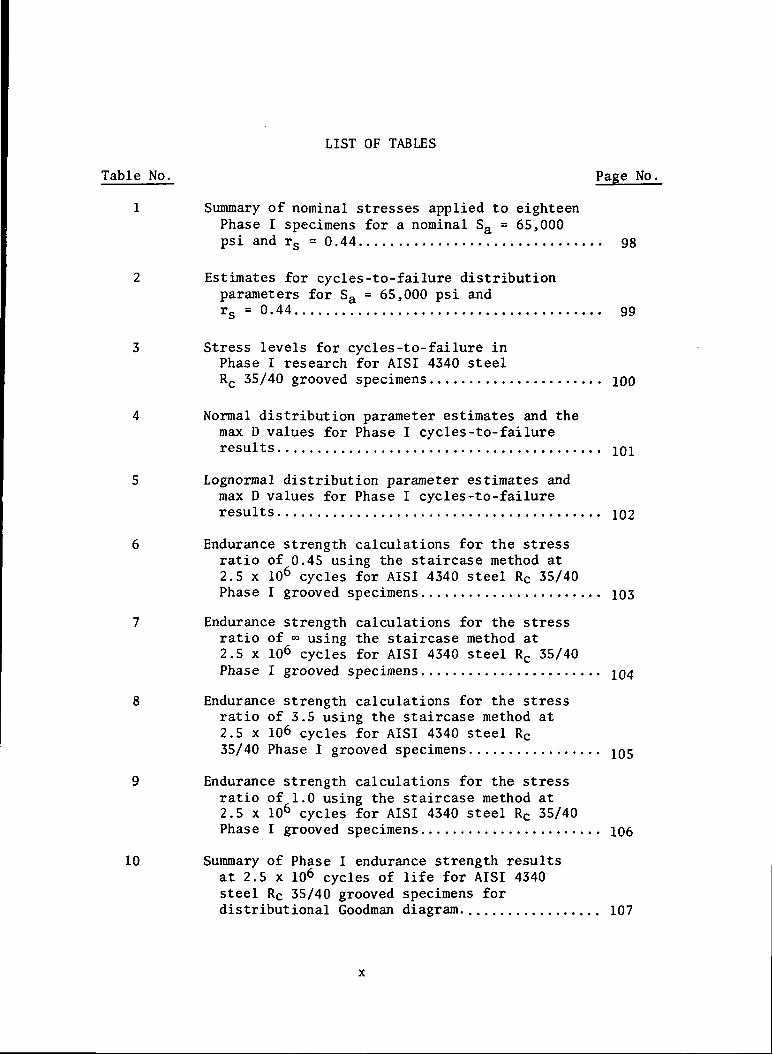
1 Summary of nominal stresses applied to eighteenPhase I specimens for a nominal Sa = 65,000psi and rs = 0.44 ............................... 98

2 Estimates for cycles -to -failure distributionparameters for Sa = 65,000 psi andrs = 0.44 ....................................... 99

3 Stress levels for cycles -to- failure inPhase I research for AISI 4340 steelRc 35/40 grooved specimens ...................... 100

4 Normal distribution parameter estimates and themax D values for Phase I cycles -to- failureresults ......................................... 101

5 Lognormal distribution parameter estimates andmax D values for Phase I cycles -to-fai lureresults ......................................... 102

6 Endurance strength calculations for the stressratio of 0.45 using the staircase method at2.5 x 106 cycles for AISI 4340 steel Rc 35/40Phase I grooved specimens ....................... 103

7 Endurance strength calculations for the stressratio of °° using the staircase method at2.5 x 106 cycles for AISI 4340 steel Rc 35/40Phase I grooved specimens ....................... 104

8 Endurance strength calculations for the stressratio of 3.5 using the staircase method at2.5 x 106 cycles for AISI 4340 steel Rc35/40 Phase I grooved specimens .................

9 Endurance strength calculations for the stressratio of 1.0 using the staircase method at2.5 x 106 cycles for AISI 4340 steel Rc 35/40Phase I grooved specimens ....................... 106

10 Summary of Phase I endurance strength resultsat 2.5 x 106 cycles of life for AISI 4340steel Rc 35/40 grooved specimens fordistributional Goodman diagram. ................. 107

LIST OF TABLES

Table No. Page

11 Diameter and surface hardness at test sectionof AISI 4340 steel Phase II ungroovedspecimens ....................................... 108

12 Diameter at the base of groove, groove radius,and surface hardness of AISI 4340 steelPhase II grooved specimens ...................... 109

13 Hardness measurements at Section A of Phase IIgrooved specimens in Rc units see Fig. 17for locations ................................... 110

14 Hardness measurements for Phase II specimensat Section A shown in Fig. 18 in R units ...... . ill

15 Tensile test data for Phase II AISI 4340 steelRc 35/40 ungrooved specimens .................... 112

16 Elongation test data for Phase II AISI 4340steel Rc 35/40 ungrooved specimens ..............

17 Tensile test data for AISI 4340 Rc 35/40grooved specimens ............................... 114

18 Summary of tensile strength parameters forPhase I and Phase II specimens .................. 115

19 Calibration coefficients and speed for eachresearch machine and for Mode 5 operation ....... 116

20 Endurance strength distribution parameterscalculations for 0.3150 in. Phase I researchAISI 4340 steel Rc 35/40 ungrooved specimensfor stress ratio of °° ........................... 117

21 Endurance strength distribution parameterscalculations for 0.2500 in. Phase IIresearch AISI 4340 steel, Rc 35/40ungrooved specimens for stress ratio of °° .......

22 Stress levels for cycles -to-failure tests inPhase II research for AISI 4340 steelRc 35/40 grooved specimens ...................... 119

XI

LIST OF TABLES

Table No. Page No.

23 Normal cycles-to-failure distributionparameters for Phase II results 120

24 Lognormal cycles-to-failure distributionparameters for Phase II results 121

25 Endurance strength calculations for PhaseII grooved specimens at stress ratioof « 122

26 Endurance strength calculations for PhaseII grooved specimens at stress ratioof 1.06 123

27 Endurance strength calculations for PhaseII grooved specimens at stress ratioof 0.40 124

28 Endurance strength calculations for PhaseII grooved specimens at stress ratioof 0.25 125

29 Endurance strength calculations for PhaseII grooved specimens at stress ratioof 0.15 126

30 Summary of Phase II endurance strengthresults at 2.5 x 106 cycles of life forAISI steel Rc 35/40 grooved specimensfor distributional Goodman diagram 127

31 K-S and Chi-squared goodness-of-fit testresults for seventeen sets of Phase IIcycles-to-failure data fitted to theWeibull distribution 128

xn

SUMMARY

This research under NASA Grant NCR 03-002-044 was initiated in

1965, and included the theoretical research for the development of an

effective methodology for designing specified reliabilities into

mechanical components,and experimental research to develop three fatigue

reliability research machines which can apply a reversed bending moment

combined with a steady torque to round, rotating, ungrooved and grooved

specimens.

Phase I of the experimental research program, initiated in 1967,

included the generation of distributional cycles-to-failure versus

alternating bending stress (S-N) diagrams and of distributional Goodman

strength diagrams for specimens made of AISI 4340 steel, R 35/40

hardness, and having a circumferential groove which provides a theore-

tical stress concentration factor, K , of 1.42.

Phase II of the experimental research program was identical to

that of Phase I except that the specimen groove provided a theoretical

stress concentration factor of 2.34, and was initiated in September 1970.

Phase II results are compared with Phase I results in this report

and the effects of superimposing a steady torque on reversed bending on

the distributional S-N and Goodman diagrams are presented, as well as the

effect of different K 's. Such distributional data has to be generated

to enable the designing of specified, target reliabilities into components.

Xlll

A methodology and a computer program were developed for the

generation of finite-life, distributional Goodman diagrams. This

methodology provides the capability for optimizing a design to achieve

a target reliability for a specified component life.

A FORTRAN computer program was developed to estimate the parameters

of the three-parameter Weibull distribution representing the cycles-to-

failure data, and to perform Chi-Squared and Kolmogorov-Smimov goodness-

of-fit tests. The program also calculates the predicted component life

for a specified reliability.

Also a study was made of the cumulative fatigue theory found in

the current literature, and a number of methods for making cumulative

fatigue reliability predictions were explored. The most promising method

of conditional probabilities is proposed for further study and verification

through a cumulative fatigue test program.

xiv

1. INTRODUCTION

1.1 Background

The research under NASA Grant NCR 03-002-044, initiated at The

University of Arizona in September 1965, included theoretical research

for the development of an effective methodology for designing specified,

target reliabilities into mechanical components and experimental research

to generate distributional, statistical S-N and Goodman diagrams to

provide the design data needed in support of this theoretical research.

During the first reporting period a basic methodology for design

by reliability in combined-stress fatigue with time dependent strength

distributions was developed. Mathematical methods in dealing with the

functions of random variables involved were discussed. Concurrently, a

supporting experimental fatigue research program was planned. It was

found that there were no research machines available which could apply to

round, rotating test specimens a combination of a reversed bending moment

and a constant torque. As a result three machines, similar in principle to

the Mabie and Gjesdahl [1] test machines were designed and built at The

University of Arizona. A complete discussion of the design and development

of the test machines was given in the report to NASA CR - 72836 [2],

During the second reporting period, the operational capability of

the first machine was proven and two additional machines were fabricated.

The design and development of, and the results obtained from, these three

machines were presented in the report to NASA CR - 72838 [3]. During the

1

2

same period calibration constants were determined for each machine so that

the nominal bending stress and the shear stress in the specimen groove can

be calculated. The calibration procedure, data, analysis, and constants

were presented in the report to NASA CR - 72839 by Kececioglu and McConnell

[4]. Calibration constants are needed because the bending and shear

stresses cannot be monitored directly. Strain gages mounted in a specimen

groove would be destroyed when the specimen failed. Hence it was necessary

to mount strain gages on the specimen holders instead of on the specimens

to monitor the bending and shear stresses. This necessitated the

determination of calibration constants and equations to relate the strain

at the strain gages to the nominal stresses in the specimen groove.

Another report by Kececioglu and Smith, NASA CR - 72835 [5], presented

all of the experimental data generated up to June 30, 1970. Included were

the reduction of the data, the application of the design by reliability

methodology, the conversion of the cycles-to-failure data to stress-to-

failure distributions, and the development of three-dimensional Goodman

fatigue strength surfaces, which is the ultimate form of the reduced data

for direct use by designers. During this period computer programs for use

in the reduction of the data were developed and refined. The most important

were program STRESS and program CYTOFR. Program STRESS calculates the

bending and shear stresses applied to each specimen, the ratio of

alternating to mean stress, and the mean and standard deviation of each

stress for each test series. It also calculates the cycles-to-failure from

the times-to-failure data recorded during the fatigue tests. Program

CYTOFR calculates the mean and standard deviation of the cycles-to-failure

for the normal and the lognormal distributions which approximate the true

distribution of the data. It then calculates the coefficients of skewness

3

and kurtosis and applies the Chi-Squared and the Kolmogorov-Smirnov

goodness-of-fit tests to determine which distribution provides a better

fit to the data.

1.2 Experimental Research

Schematic diagrams of the NASA Complex-Fatigue Research are shown

in Figs. 1 and 2. A test specimen is subjected to a bending moment by

weights hung at the end of a lever arm. Torque is applied through the

Infinit-Indexer which rotates shaft A with respect to shaft B and holds

the relative position of the shafts. Two four-arm strain gage bridges are

mounted on the toolholder in the positions shown in Figs. 3 and 4. The

output of one bridge is proportional to the strain resulting from the

alternating bending stress, and the output of the other bridge is

proportional to the shear strain resulting from the steady torque. The

numerical relationship between the strains measured at the toolholder and

the nominal stress in the specimen groove is established through the

calibration program discussed by Kececioglu and McConnell [4].

Two types of tests are conducted: One to determine the cycles-to-

failure distribution at a given alternating bending stress level and

bending to shear stress ratio. The other to determine the endurance

strength, or stress-to-failure, distribution. The steps involved in each

type of test are summarized in Fig. 5. A bending stress level and a

stress ratio are selected from the overall test program and

*assigned to one of the three research machines. A PDP-8 computer program

is run to determine the corresponding shear stress and the number of

Visicorder divisions required to represent the bending and shear stresses.

The Visicorder records the amplified outputs of the strain gage bridges.

See Appendix A.

4

The test sequence begins with the installation of a specimen in the

toolholder collets, with the groove centered between the collets. With

the collet on the strain gage side tightened, the instrumentation is

zeroed and calibrated. After tightening the other collet, weights are

added to the bending-load arm, and the torque is applied to obtain the

desired stresses as indicated by the number of divisions on the Visicorder.

At this time a microswitch, which stops the machine when the specimen

fails, is set and an interconnected clock is set to zero. The machine is

then started, and run at constant speed until the specimen fails. The

time to failure is recorded and subsequently used to calculate the number

of cycles to failure for that specimen. After running 35 specimens at

the specified nominal bending stress level and stress ratio, a data deck*

is prepared for program STRESS to be run on a CDC-6400 Computer. The

program inputs include the time to failure, Visicorder resistances and

divisions used for its calibration, and the divisions recorded during each

specimen for the bending and shear stress levels. The program calculates

the achieved bending and shear stresses, stress ratio, and cycles to failure

for each one of 35 specimens used in each test series. Then it calculates

the statistical mean and standard deviation of the bending stress, shear

stress, and stress ratio achieved in each test series of 35 specimens.

The cycles to failure of each specimen becomes the input into program**

CYTOFR for analysis of the statistical distribution of the 35 cycles-to-

failure data. The normal and lognormal distribution parameters are

determined, as well as.-the skewness, kurtosis and the Chi-Squared and

Kolmogorov-Smirnov goodness-of-fit test results. The lognormal distribution

parameters are then used to construct the distributional S-N diagrams.

* See Appendix B.** See Appendix C.

5

The Weibull distribution having gained favor recently in fatigue

studies, it was decided to determine the parameters of the Weibull dis-

tribution that represents the cycles-to-failure data. PROGRAM WEIBULL

is now used to accomplish this and to see which one of the three

distributions (normal, lognormal, and Weibull) represents the cycles-

to-failure data best.

The staircase method of testing is used to determine the stress-

to-failure, or endurance strength, distribution parameters. The

endurance strength is taken to be normally distributed, and is plotted

along with the cycles-to-failure distributions to complete the distri-

butional S-N diagrams. The staircase results are also used to construct

the very valable distributional Goodman diagrams.

The experimental research for this reporting period consisted

of completing the test program planned for Phase I, consisting of cycles-

to-failure testing at a stress level of 65,000 psi at the stress ratio

of 0.44 and endurance strength testing, to complete the S-N and Goodman

diagrams for Phase I research.

In addition the Phase II research was undertaken. The

experimental research of Phase II was a continuation of the research

performed in Phase I, but with new test specimens.

The Phase I specimens, shown in Fig. 6 were shafts made of

AISI 4340 steel, MIL-S-5000 B, Condition C-4, Rockwell C 35/40, grooved

to provide a theoretical stress concentration factor of 1.42. The

specimens for Phase II, shown in Fig. 7, are identical to the Phase I

specimens except that they have a different groove geometry to provide

* See Appendix D.

6

a theoretical stress concentration factor of 2.34. The results of this

research are presented here and compared.

Much valuable fatigue reliability design data has thus been

generated experimentally in support of the theoretical methodology for

designing specified reliabilities into rotating components subjected

to combined reversed bending and steady torque.

On the theoretical side a methodology for generating finite

life distributional Goodman diagrams was developed. In addition a

promising method to calculate the reliability of rotating components

subjected to cumulative fatigue loads was developed and is presented

here.

2. EXPERIMENTAL RESEARCH

2.1 Phase I Research Completion.

The results of Phase I experimental research accomplished prior to

this period were reported by Kececioglu and Smith [5]. They included

endurance tests at stress ratios of °°, 3.5 and 0.83. Cycles-to-failure

tests were accomplished at two alternating stress levels for the stress

ratio of 0.44: 69,000 psi and 60,000 psi. The endurance run for the

stress ratio of 0.44 was also begun during the previous reporting period

but was not completed.

Another cycles-to-failure test series for the stress ratio of 0.44

with eighteen (18) specimens was run on Machine No. 1 at a nominal bending

stress level of 65,000 psi. Program STRESS was run on the CDC-6400

Computer to determine the nominal bending and torque stresses in the groove

of the specimen and the resulting stress ratio achieved in these tests.

The results are summarized in Table 1. From Table 1 it can be seen that

the achieved standard deviations are approximately two percent of the mean

values of the stresses and the stress ratio. The run was, therefore, under

control, and the test results were considered acceptable.

The cycles-to-failure calculated by program STRESS for each specimen

were used as inputs into program CYTOFR for the analysis of the distribution

of the data. A summary of the outputs from the program is shown in Table 2.

8

A comparison of the goodness-of-fit results obtained for the

normal and lognormal distributions shows the following:

1. The K-S test does not reject either distribution since the

maximum D value is less than the allowable in each case.

2. The coefficient of skewness is significantly larger than

zero for the log cycles than for the straight cycles; where

the coefficient of skewness of the symmetrical normal dis-

tribution is zero.

3. The coefficient of kurtosis for the data fitted to a normal

distribution is smaller than the value of 3.0 for the normal

distribution, and the value obtained for the lognormal dis-

tribution is greater than 3.0.

Based on the overall statistics and the conformance of previous

results, the lognormal distribution was chosen. The results are plotted

in the S-N diagram of Fig. 8. Figs. 9, 10, and 11 give the S-N diagrams

-for the previous research results of purposes of completeness and

comparison. Table 3 summarizes the results used to obtain Figs. 8 thru

11. Table 4 summarizes the results of the normal distribution fit to

all Phase I cycles-to-failure data and Table 5 of the lognormal dis-

tribution fit, for purposes of completeness and comparison.

Tests to determine the endurance strength for the stress ratio

of 0.44 were run on Machine No. 2. The staircase method [5, p. 19]

was used with specimens tested to 2.5 x 10 cycles for success.

* The stress ratios actually achieved in these tests averaged out to

r =0.45, consequently these endurance strength results are reported

as being for r =0.45.

The results for 37 valid data points are shown in Fig. 12. Using the

equations presented in Mood and Dixon [8, p. 114] the mean and

standard deviation of the endurance strength distribution were calcu-

lated, as shown in Table 6, giving an endurance strength mean of

49,600 psi and a standard deviation of 3,700 psi. The results obtained

from the cycles-to-failure tests and the endurance tests were used to

complete the S-N diagram shown in Fig. 8.

The endurance strength distribution parameters were applied to

equation [5, p. 37] .

-Sr = Sa (1 + Tr

and

r a r

to obtain the parameters of the distribution along r = 0.45, with

the following results:

S = 120,900 psi,

and

o = 9,000 psi.Or

The incorporation of this r =0.45 strength distribution into

the Goodman diagram shown in Fig. 13 completed the distributional

Goodman diagram for 2.5 x 10 cycles of life and the Phase I experi-

mental research program. Figures 14, 15, and 16 give the staircase

test results for r = °°, 3.5, and 1.0 respectively; and Tables 7, 8,

and 9 give the corresponding calculations of the endurance strength

distribution parameters for purposes of completeness and comparison.

10

Table 10 summarizes the endurance strength results used to prepare

Fig. 13.

2.2 Phase II Research

The Phase II experimental research objective was to obtain

distributional S-N and Goodman diagram data with specimens of the

same steel as for Phase I but having a theoretical stress concentration

factor of 2.34 instead of 1.42 for Phase I.

2.2.1 Geometry and Hardness of Research Specimens

Fig. 7 shows the geometry of the new specimens. The

manufacturing processes were carefully controlled, to assure metallur-

gical and strength similarity to Phase I specimens. Accordingly

thirty-five (35) 9" long ungrooved specimens and thirty-five (35) 9"

long grooved specimens for use in tensile tests, and one-thousand-

fifty (1,050) 6" long specimens for use in fatigue testing were obtained.

Measurements were made of the ungrooved and grooved

specimens to verify the contractor's ability to meet machining tolerance

and hardness requirements. The first set of tensile test specimens

were not acceptable when the hardness and base diameters were found

not to be within specifications, and the yield and ultimate strengths

of the ungrooved specimens were significantly lower than those for the

Phase I specimens.

To assure that Phase I and Phase II specimens, made of

two different lots of AISI 4340 steel, were similar except for the

change in groove size and its effect on strength, a second set of

11

tensile test specimens was obtained. The specimen diameters and radii

were measured with an Optical Comparator, at 20 magnification, located

at the Arizona Gear Co. in Tucson. The results are given in Tables 11

and 12. The surface finish at the base of the groove of the grooved

specimens was observed through a microscope and visually compared with

Johansen's precision gage blocks made by Pratt and Whitney because of

the inaccessibility of the base of the groove to a Profilometer.

Surface hardness measurements were made in the University's Metallur-

gival Laboratory with a Wilson Rockwell C Hardness Tester using a

150-K load and the Braile indenter. The results are given in Tableso

11 and 12. In addition, hardness tests were made on interior cross

sectional areas of three grooved and three ungrooved specimens to

determine the uniformity of hardness throughout each specimen.

Standard precautions were taken to assure that the original hardness

was not altered during sectioning. The location of test sites for the

interior hardness measurements are shown in Figs. 17 and 18. The

results of the interior hardness measurements are given on Tables 13

and 14.

Applying a 3o analysis to the surface hardness data in

Tables 11 and 12 indicates that 99.73% of the population would lie

between the limits of 36 R and 39 R for the grooved specimens, and

between 35 R and 39 R for the ungrooved specimens, hence within the

specifications of R 35/40. The hardness readings in the sections

given in Tables 13 and 14, show a preponderance of values between

35.5 R and 37.5 R with a high degree of uniformity. Since thet» C»

hardness at the surface and in the interior of the specimens met the

12

specification requirements of R 35/40, it was concluded that thec

specimens were given a proper heat treatment.

2.2.2 Strength Characteristics of Research Specimens

The ungrooved and grooved specimens were subjected to

tensile loads to determine their yield, ultimate and breaking strengths.

The tensile pull tests were performed at the Hughes Aircraft Company,

Tucson, Arizona on a 60,000 Ib. Tinius Olsen test machine. The machine

was calibrated a short time before the tests and was considered to be

in a fully operational condition.

The thirty-five (35) ungrooved specimens were tested

with an extensometer attached to each specimen which provided elong-

ation input to a load-elongation pen recorder. The load was con-

currently displayed on a 30-in. diameter dial segmented into to psi

intervals on the 0 - 60,000 psi scale. The elongation of a two-inch

gage length was measured with a micrometer after the specimen failed,

and the percent elongation was calculated.

As the specimen was placed under tension at a constant

rate of elongation, observers watched the dial in an effort to identify

the yield, ultimate and breaking loads. Upon reaching the ultimate

point, the specimen was unloaded, the extensometer was removed, and

the specimen diameter was measured with a micrometer to determine any

reduction in cross-sectional area. The load was reapplied and the

specimen was stressed to the breaking point. The yield load was

identified on the recording at the 2% elongation point and the ultimate

load was identified by the maximum load recorded on the chart. The

13

load at the breaking point, determined by visually observing the moving

pointer, was manually recorded. The yield, ultimate, and breaking loads

thus obtained are given in Table 15 and the percent elongation data

and results are given in Table 16.

After completion of the tensile test, the diameter of

the ungrooved specimens were remeasured on the Optical Comparator to

determine the area to be used in calculating the breaking strength.

The final diameters and the elongation measurements are given in Tables

15 and 16. The yield and ultimate strengths were calculated using

the original (pre-test) specimen diameters; whereas, the breaking

strength, was calculated on the basis of the final (reduced by elongation)

diameters. The results are given on Table 15 and are summarized at the

end of Table 15.

During the testing of the grooved specimens the

extensometer could not be used and the dial readings were visually

observed and manually recorded. During the test of the first specimen

it was observed that (1) the yield load could not be positively ident-

ified, (2) there was little time lag and reduction in load between the

ultimate and the breaking loads, and (3) the actual fracture of the

specimen was accompanied by a. loud shock wave throughout the testing

laboratory. A decision was made thereafter to unload the specimens

after the ultimate load was reached. Thus only the ultimate loads could

be obtained, and are given in Table 17. Any change in specimen diameter

at the ultimate load could not be measured accurately enough, hence

it was decided to use the original (pre-test) area to calculate the

14

ultimate strength. The results are given in Table 18, and a\

summary thereof is given at the end of Table 17.

2.2.3 Analysis of Tensile Test Results

Before making the final decision regarding the accept-

ability of the tensile test specimens as a basis for procuring fatigue

test specimens, a review was made of the strength parameters obtained

from test of the Phase I and Phase II specimens. The strength para-

meters of the Phase I tensile test specimens, extracted from our

previous report [3, Tables 7 and 8], and the results of the Phase II

tests just discussed are listed in Table 18. It is noted that the

mean yield and ultimate strengths obtained from Phase II tensile tests

of ungrooved specimens are lower than the yield and ultimate strengths

of the Phase I specimens. The standard deviations are different but

within 4 percent of the respective means. The ultimate strength for

the grooved specimens of Phase II was higher than for Phase I. This

should be expected because Phase II specimens have a smaller groove

radius which results in a higher static ultimate strength; consequently,

this does not provide a basis for believing that the Phase II and

Phase I specimens are different.

The student "t" test was used to perform a comparison

of the sample means of the ultimate strengths of the Phase I and

Phase II tensile test specimens [7, pp. 193-194]. This method was

selected because it is widely accepted to be valid for small sample

sizes, and the Phase I data means were based on a sample size of 10.

The results of the statistical tests and the corresponding critical

15

values at the 0.05 level of significance are as follows:

t - Statistic t - Statistic

Critical Value

Ungrooved Specimens 19.65 2.02

Grooved Specimens 13.10 2.02

The t-statistic is larger than the t-critical value which indicates

that the difference between the means of the ultimate strength is

statistically significant. The Phase I ungrooved specimens are

apparently the stronger.

The sample variances of the ultimate strengths were

compared using the F-test [8, pp. 167-172]. The results, at the 0.05

level of significance, are as follows:

F - Statistic F - Statistic

Critical Value

Ungrooved Specimens 3.00 2.84

Grooved Specimens 1.08 2.85

The F-test for the variance further indicated a significant difference

between the Phase I and Phase II ungrooved specimens but not between

the grooved specimens.

The results of the statistical analysis do not provide

a logical basis for accepting or rejecting the Phase II specimens.

Thus it became necessary to use different criteria to determine the

acceptability of the tensile test specimens as a basis for ordering

fatigue test specimens.

16

A metallurgical analysis of a specimen was obtained to

determine its composition as AISI 4340 steel and its compliance with

MIL-S-5000B. The analysis performed by Magnaflux Corporation, Materials

Testing Laboratories confirmed that the sample met all requirements for

the chemical composition.

A review of the data from the physical measurements

given in Tables 11 thru 14 confirmed that the test specimens met all

specification requirements. The hardness values, which are considered

to be most critical are well within specification requirements for

surface hardness, and the additional hardness measurements on interior

cross sectional surfaces also confirmed the uniformity of the hardness.

All factors considered, the decision was made to proceed with the pro-

curement of fatigue test specimens for Phase II.

2.2.4 Recalibration of NASA Complex-Fatigue Research Machines

2.2.4.1 Requirements

Machine No. 2 required recalibration since it

had been modified by the installation of spherical bearings at

the Flex Couplings. Machines 1 and 3 were also recalibrated

so that the strain gages of all machines would be verified to

be functioning properly, and to revise the calibration co-

efficients if the calibration results so indicated. The speed

of each machine was also measured to assure its constancy and

to determine if any change occurred due to wear in each machine

and its drive motor.

17

2.2.4.2 Procedures and Results

The calibration method and procedures used

were the same as those described in NASA CR - 72839 [4, pp.

30-33]. The bending calibration was accomplished in two

phases. First an out-of-machine bending calibration was done

using the setup shown in Fig. 19. This phase verified that

the bending bridge strain gages, shown in Fig. 3, mounted on

the toolholder arm of each machine and the strain gage mounted

in the groove of the calibration specimen were functioning

properly and provided a relationship between the actual and

the apparent strain in the toolholder strain gages. This was

based on the facts that the actual/apparent stress ratio was

close to the one it should be, and the plot of strain from the

gage bridge versus applied weight was linear.

The test setup shown in Fig. 20 was used to

determine the calibration coefficients for the torque bridge,

shown in Fig. 4, and for any interaction between torque and

bending bridges.

Next an in-machine, quasi-dynamic calibration

was performed which provided the calibration coefficient needed

to calculate nominal bending stress in the specimen groove

from the apparent stress at the toolholder.

Each machine was carefully calibrated with

observations repeated a minimum of six times at each test

point. The relation between the calibration variables, in

each case, proved to be linear with the functional relationship

18

beginning at the origin. Thus the slope of each regression

line for the calibration data completely defined the function

and provided the calibration coefficients listed in Table 19.

The rotating speed of each machine was

determined using a tachometer strobe light which contains an

internal oscillator and 60-cycle calibration. The results

confirmed proper operation of each induction motor in providing

a constant speed drive to each research machine. It was also

found that the speed of each machine was independent of the

bending and torque loads. The speed of each machine is listed in

Table 19. The last calibration coefficients of the previous

calibration was designated as Mode 4. The coefficients

designated as Mode 5 apply to all data from June 1, 1971 until

the next calibration.

2.2.5 Ungrooved Specimens Fatigue Research

Thirty-five Phase I specimens were machined down as

shown in Fig. 21 so as not to provide any stress concentration at all.

These specimens were tested in the Ann Arbor (R. R. Moore type)

rotating beam fatigue research machine in our Reliability Research

Laboratory to determine the endurance strength of ungrooved specimens.

An optical comparator was used to determine the point

of minimum diameter of each specimen and to measure the diameter. It

was found that the specimens had a mean diameter of 0.3151 in., a

standard deviation of 0.0004 in., and a range of 0.3143 in. to 0.3159

in.

19

A computer program was written and executed on the

PDP-8 Computer to calculate the bending moments and pan loads required

to test ungrooved specimens at target stress levels and desired

specimens diameters.* The program was based on the following cali-

bration equation for the Ann Arbor machine:

M = 0.267 + 4.09L (3)

where

M = bending moment at the test section

L = total effective load = pan weight (P) + 8.625 Ib.

Therefore the pan weight, P, to obtain a bending moment, M, is given

by

P - CM + °-267) *P " - 4709 - ' 8<

where

,. TT D x Stress ,cM = - - • (5)

and D is the test section diameter of the specimen to be tested next.

In view of the range of specimen diameters, the

computer program was run to calculate pan loads at diameter intervals

of 0.0005 in. from 0.3140 in. to 0.3160 in. for each stress level

desired. With interpolation, the required pan weights could be

determined to the nearest +_ 0.10 Ib.

The staircase method of determining the endurance

strength was used with a stress increment of 1,900 psi and a life of

2.5 x 10 cycles. A specimen was selected at random, its diameter

obtained from the table of specimen diameters, and the appropriate pan

* This program is given in Appendix F.

20

weight as determined from the PDF program printout was used to apply

the desired stress level.

Thirty-eight valid runs were completed, as shown in

the staircase plot of Fig. 22, with 15 successes and 13 failures.

These data were then used to calculate the mean and standard deviation

of the endurance strength distribution at 2.5 x 10 cycles of life for

the AISI 4340 steel, R 35/40, ungrooved specimens subjected to an

alternating bending stress and a constant shear stress with a shear

ratio of r = <*>, as shown in Table 20. The mean endurance strength

was found to be 80,725 psi and the standard deviation 3,040 psi. In

comparison, the published endurance strength is estimated to be approx-

imately 89,000 psi for polished specimens and 81,000 psi for machined

specimens [9, pp. 160-172]. The mean endurance strength as determined

by this test program is very close to the published endurance strength

of polished specimens. Thus the results of the tests are reasonable

and compatible with current fatigue failure theory.

When the decision was made to procure a second group

of tensile test specimens, it was decided to obtain another group of

ungrooved specimens and repeat the above tests to provide another

basis for accepting the Phase II specimens as having physical prop-

erties close to those of Phase I specimens. A number of Ann Arbor

research machine outages had been encountered because the bending

moments at higher stress levels approached the limit of the machine.

Thus, it was decided to reduce the diameters of the new specimens to

a nominal value of 0.2500 in. Thiry-five Phase II research specimens

were obtained as per Fig. 21. The diameter of the specimens were

21

measured at the minimum point and the mean diameter was found to be

0.2504 in. with a standard deviation of 0.0004 in. A specimen was

randomly selected and the appropriate pan weight was determined from

the PDF Computer program as before. The endurance life was again

taken to be 2.5 x 10 cycles and the staircase stress increment 1,900

psi.

Thirty-four useful data points consisting of 18

successes and 16 failures were obtained, as shown in the staircase

plot of Fig. 23. The 16 failures were used in the calculations given

in Table 21. The endurance strength distribution parameters of the

0.2500 diameter, ungrooved, Phase II research specimens subjected to

an alternating bending stress and no shear stress, with a stress ratio

r = °°, were found to be: Mean = 80,230 psi, and standard deviationo

= 1,425 psi. As the mean endurance strength was identical for both

Phase I and Phase II steel specimens, the decision to continue using

this steel and the manufacturer of the research specimens for the

Phase II research was upheld.

2.2.6 Grooved Specimens Fatigue Research

2.2.6.1 Cycles-to-Failure Tests

The Phase II test program using the new

specimens, grooved to provide a theoretical stress concentration

factor of 2.34, was initiated at the stress ratio of infinity.

Using the von Mises-Hencky failure theory, the stress ratio ,

rs, for the loading provided by the research machines used in

this research, is defined as

22

rs = —-* (8)/3 Txym

where

S = alternating reversed bending stress due to the bendinga

moment.

T = mean shear stress due to torque.xym n

Cycles-to-failure tests at the stress ratio of infinity

were conducted at mean nominal alternating stress levels of 108,900,

92,100, 73,600, 49,400, and 39,300 psi. Five stress levels are chosen

to obtain data over the finite life range for the preparation of the

corresponding S-N diagram.

Upon completion of testing at the stress ratio of

infinity, a decision was made to conduct all fatigue tests at a

specific ratio on one test machine. Therefore, tests were initiated

and completed at stress ratios of 1.06, 0.40, 0.25, and 0.15. Fewer

stress levels were run as shown in Table 19 for stress ratios lower

than °° because of yield stress limitations in shear.

The sample size to obtain the cycles-to-failure

distribution for each alternating stress level and stress ratio com-

bination was increased to 35, as recommended in the previous report

[5, p. 95]. The actual alternating bending stress, the shear stress,

the normal mean stress, and the stress ratio for each specimen in the

sample were calculated by computer program STRESS. In addition, the

mean and standard deviation of the achieved stresses for each sample

were calculated, and are given in Table 22.

23

Program STRESS was updated for Phase II to incorporate

current calibration constants for each machine to reduce the test data,

and add rpm values for each machine. The computer printout includes

a listing of the cycles to failure for each specimen in the sample.

The updated program in Fortran language is given in Appendix B.

Individual cycles-to-failure data were used as input

data for program CYTOFR, as discussed in the previous report to NASA

[5], to calculate the cycles-to-failure distribution parameters for

the normal and log normal distributions and perform goodness-of-fit&

tests. Program CYTOFR was further updated to incorporate Cal-Comp

graph and plot subroutines. Subroutine GRAPH constructs a histogram

of the cycles to failure based on the failures per cell determined by

the Chi-Squared test, and superimposes the distribution curve from the

parameters computed by the main CYTOFR program on each histogram. The

Chi-Squared test modification incorporated the automatic combining of

cells at the tails of the distribution when the end cells do not

contain at least five failure data points. The updated program in

extended Fortran language is given in Appendix C.

Program CYTOFR was run for each alternating bending

stress level at which specimens were tested at the stress ratios of

infinity, 1.06, 0.40, 0.25 and 0.15. Typical examples of the histograms

and curves for the normal and log normal distributions are given in

Figs. 24 and 25. The computed distribution parameters and values of

the goodness-of-fit tests are summarized in Table 23 for the normal

distribution, and in Table 24 for the log normal distribution.

24

The goodness-of-fit test parameters listed in these

tables were reviewed to determine if the applicable distribution of

the cycles-to-failure data for Phase II specimens differed significantly

from that for Phase I specimens. The following observations were

made:

1. The values of the coefficients of skewness and kurtosis

for the normal and the lognormal distributions were

approximately the same and provided no preference for

either distribution.

2. The K-S goodness-of-fit test does not reject either

distribution at the 0.05 level of significance. The

largest D value was 0.201 for the normal distribution

and 0.160 for the lognormal distribution; both were less

then the critical D value of 0.224 at the 0.05 level

of significance for a sample size of 35. Furthermore,

there was essentially no difference between the normal

and lognormal D values at any stress level.

3. The Chi-Squared test proved to be more discriminating

than the K-S test. The Chi-Squared value and the

appropriate degrees of freedom (d.o.f.) for each stress

level were compared with the critical value of 3.841

for 1 d.o.f. and of 5.991 for 2 d.o.f. . The normal

distribution was rejected in three out of seventeen

samples; and the lognormal distribution was rejected

in only two out of seventeen samples. One test each

for normality and lognormality was inapplicable because

25

the data points were contained in only three cells

resulting in zero degrees of freedom.

4. It was concluded from these observations that there is

a preference for the lognormal distribution over the

normal distribution when working with cycles-to-failure

data.

The log normal distribution parameters from Table 24C

were used to construct the S-N diagrams for the Phase II

specimens. These S-N diagrams are given in Figs. 26 thru

30.

2.2.6.2 Endurance Tests

Endurance runs for Phase II specimens were

completed using the "staircase" method at alternating bending

to mean shear stress ratios of », 1.06, 0.40, 0.25 and 0.15.

The staircase plots are given in Figs. 31 thru 35. The

endurance strength distribution parameters were calculated in

Tables 25 thru 29, and are summarized in Table 30. These

parameters were used to complete the S-N diagrams of Figs. 26

thru 30, and to construct the distributional Goodman diagram

of Fig. 36.

26

3. THEORETICAL RESEARCH

3.1 Generation of Finite Life Distributional Goodman Diagrams for

Reliability Prediction

A methodology for developing finite life distributional Goodman

strength surfaces from cycles-to-failure distributions at specified

alternating stress levels has been developed by Kececioglu and

Guerrieri [10]. The Goodman strength surface shows the combinations

of alternating bending stress and mean shear stress allowable to the

design engineer. This study also investigated the applicability of the

distortion energy and the maximum shear stress failure theories to

determine which provided better correlation with the experimental

data generated during Phase I. The finite life Goodman surface,

developed using from two to five calculated strength distributions at

specified stress ratios, can be used to construct distributions at any

desired stress ratio and applied to probabilistic design.

It is also found that the von Mises-Hencky ellipse effectively

models Goodman diagrams for life greater than 10,000 cycles. However,

when the equation for the von Mises-Hencky ellipse was modified from

to

• ' fl0)

and the values of a were determined from plots of finite life Goodman

diagrams, the values ranged from 1.91 at 200,000 cycyles to 2.38 at

27

40,000 cycles. This is an area that requires further study in search

of a general equation, or applicable values of a, valid over all

ranges of cycles to failure.

3.2 The Weibull Distribution as A Description of Fatigue Life

3.2.1. Introduction

Since the Weibull distribution was introduced in 1949,

it has gained wide acceptance as an extreme value distribution [11].

It has been used extensively in such areas as bearing fatigue data

analysis [12], and the prediction of the failure of automotive parts.

The Cal-Comp plots of normal and lognormal distributions

did not fit the cycles-to-failure data very well for some sets of

data. It was suggested that the three-parameter Weibull distribution

may provide a better fit.

The theory of the Weibull distribution and its manual

application to experimental data are described in the existing

literature [11], [12]. This study developed and validated a computer

program which computes the parameters of the three-parameter Weibull

distribution for a set of cycles-to-failure data, performs goodness-

of-fit tests, and calculates the cycles to failure for 0.90 and

0.99 reliability with 90% confidence. The program was tested using

the data generated under Phase II and the results were analyzed.

28

3.2.2 Development

The computer program development was patterned after the

method described by Lochner [12], which used Weibull probability paper

and manual calculations. The foundation is the generalized Weibull

frequency distribution shown in Hahn and Shapiro [11, p. 110]

f(N; 3, n,

> Y, - O ° < Y < O , B > o, n > o ,

where

N = cycles to failure

6 = shape parameter or Weibull slope

n = scale parameter

Y = location parameter .

From the basic definition of reliability

f(N) dN,N

the relationship between reliability and fatigue life N is

R = e n , (12)

where Y» i» a°d 3 are constants to be determined by the analysis of

test data. The fraction failed, or unreliability Q, for N cycles

is given by

29

Q = 1 - e " " / . (13)

Equation (13) gives the probability of failure in N cycles or less, and

is the cumulative distribution function, F(N). It can be transformed

into a linear form by taking natural logarithms as follows:

F(N) = 1 - e

1 - F(N) = e

and

/ N - Y\ P~\ n / ,

In In [1 _1p(N) ] = e In (N - y) - 6 In n. (14)

Letting

Y = I" I" [} . F(N)] •

and

x = In (N - Y), (16)

Eq. 14 becomes

y = 3 x + constant,

or a transformed linear function.

Weibull probability paper has been prepared with log log versus

log scales so that the plot of y versus x of data would be a straight

--line with a slope of 6. When (N-y) = n, F(t) = l-e \r\ J =1

-1 ~- e = 0.632, thus the value of (N-Y) at which F(N) = 0.632 is an

estimate of n- The location, parameter, Y» is the minimum life point

that provides the best approximation to linearity between x and y.

30

3.2.3 Weibull Computer Program

The basic FORTRAN computer program to determine the

estimates of the Weibull parameters for cycles of life for specified

levels of reliability was provided by Mr. Thomas C. Stansbefry, Delco

Radio Division, General Motors Corporation. His program was adapted

to The University of Arizona CDC 6400 Computer and was updated to

include subroutines for the Chi-Squared and Kolmogorov-Smirnov goodness-

of-fit tests. Program WEIBULL is given in Appendix D.

The first data card contains the sample size and the

minimum life increment for use in linearizing the x-y relationship.

Subsequent data cards (one for each specimen) contain the cycles-to-

failure information. The first operation performed by the computer is

to establish an ordered array of the cycles to failure and the

corresponding median ranks. The computer calculates the median ranks,

y± = In In (_JL_), and x± = In (1^ - Y]c). Where i = 1, 2, —,

n and y, = minimum life increment (1, 2, }k) such that y, < N.. As

the array of y. and x. is computed for different y, the method of1 1 K

least squares is used to determine the degree of linearity. This

operation is iterated with y. being increased in increments until theK

best fit straight line is obtained. At that time the computer

records the estimates of y, 3, and n. It then calculates the one

percent failing life, the ten percent failing life, and the 50 percent

failing life with the associated 90 percent confidence limits.

Upon completion of the calculations, the program calls

the K-S and Chi-Squared test subroutines, in turn, to provide a

measure of goodness of the fit of the estimated Weibull distribution

31

with the data. The K-S subroutine, "DTEST", applies the Kolmogorov-

Smirnov goodness-of-fit test and prints differences, D, for each

, failure time in ascending order. Analysis of the K-S test is done by

comparing the largest in absolute D value, with its critical value

obtained from a D value table.

The Chi-Squared test requires the subdivision of the cycles-to-

failure data into a number of cells, k, determined by Sturges1 rule

[13]

k = 1 * 3.3 log10 (n) , (17)

Where n is the sample size of the data. However,

analysis of the results requires at least five data points in each

cell. The use of Sturges' rule for data with a sample size of 35,

results in six cells of equal width. Consequently, when the data is

grouped into these six cells the cells at each end usually end up

with fewer than five data points. If the two end cells are combined

to provide five or more data points, the number of filled cells reduce

to as few as four. Since the distribution being tested is the three

parameter (r=3) Weibull, the degrees of freedom (k-r-1) requires that

the number of cells, k, be at least five in order to have at least one

degree of freedom. This Chi-Squared test was applied to samples of

Phase II cycles-to-failure data. It was found that six of the

twelve tests resulted in only four filled cells. Thus, there was zero

degrees of freedom and the Chi-Squared test was not useable. Thus,

it appears that the sample size will have to be increased still further

if the standard Chi-Squared goodness-of-fit test is to be used.

32

To circumvent this problem variable cell widths were

used. The technique described by Hahn and Shapiro [11, pp. 302-308]

called for the calculation of cell widths to provide equal number of

observations in each cell. A modification to the subroutine was made

dividing the range of the data so that each cell contains exactly five

cycles-to-failure data. For our sample size of 35, this provides

seven cells. This subroutine was run for the same 12 sets of data.

The expected frequency for the seventh cell was always less than five,

which according to accepted practices invalidate the test. It was

observed, however, that as long as the expected frequency was equal

to or greater than two, the Chi-Squared value could be calculated.

This observation was confirmed by a Monte Carlo Simulation of 1,000

runs from which it was concluded that Chi-Squared errors resulting

from expected frequencies between two and five are insignificant.

Nevertheless, a final modification was made to the subroutine using

variable cell widths, but combining adjoining end cells to insure that

the expected number of observations per cell is equal to or greater

than five. When the same cycles-to-failure data was rerun to apply

this Chi-Squared test subroutine, all 12 tests resulted in six useable

cells thus providing two degrees of freedom.

3.2.4 Results

The operation and accuracy of the computer program were

verified by using the same input data used by Lochner [12]. Identical

estimates were obtained for each parameter to the degree of accuracy

obtainable from probability paper plots. The computer program

33

provided parameter estimates to five place accuracy and used this

accuracy in subsequent calculations. In Table 31 the Weibull distri-

bution parameters, and the K-S and Chi-Squared goodness-of-fit results

are given. A sample Cal-Comp plot of the Weibull distribution is given

in Fig. 37.

The accuracy of the D-test subroutine for the Kolmogorov-

Smirnov goodness-of-fit test was confirmed by a desk calculator. The

maximum D values found by applying the subroutines to the cycles-to-

failure data are listed in Table 31. These results show that, at the

0.05 level of significance, the K-S test does not reject the Weibull

distribution in all of the 17 tests. Thus, the Weibull distribution

can safely be used to approximate distributions of cycles-to-failure

data at specified stress levels.

The Chi-Squared test values determined by the WEIBULL

subroutines with variable cell widths are also given in Table 31.

Note that the variable cell width analysis rejects 5 out of 17 tests.

The conclusions drawn from the above analysis are listed

below:

1. Based on the K-S test results of not rejecting any of the

samples, the three-parameter Weibull distribution may

describe fatigue cycles-to-failure data.

2. Based on the Chi-Squared test results of 5 rejections out

of 17 samples, the Weibull distribution may not be

considered generally acceptable for cycles-to-failure data

consisting of 35 data points. Further in 14 out 16 cases

34

the Chi-Squared value for the Weibull is greater than for

the lognormal.

3. Based on the previous two conclusions and the results in

Tables 24 and 31, the lognormal distribution appears to

represent the cycles-to-failure data of the Phase II

research best.

3.3 Reliability of Components Subjected to Cumulative Fatigue

3.3.1 Introduction

In cumulative fatigue of most concern to design

engineers is the mathematical relationship between the number of load

cycles at various alternating stress levels applied to a component,

the S-N diagram results, and the survival life of the component under

these conditions. After such a relationship is determined a method

needs to be developed to predict the reliability of a component sub-

jected to a specified history of cumulative fatigue stresses. The

objective of this study was to review the published cumulative fatigue

theories, and to discover or come up with methods for making reliability

predictions.

35

3.3.2 Literature Search

The literature search revealed attempts to describe the

degree of cumulative damage in expressions involving transfer of

energy or mass, with damage often described by a crack parameter and

interpreted by Osgood [14] as a change in the state of energy in the

immediately adjacent volumes of material. The primary difficulty

with these methods is their complexity and highly approximate nature.

The simplest and most widely used cumulative damage rule

is Miner's rule [15], based on the assumption that cumulative damage

under cyclic stressing is related to the net work absorbed by the

specimen. That is, the number of stress cycles applied, expressed as

a percentage of the number of cycles of life at the given alter-

nating stress level, is the proportion of useful life expended.

Therefore, the specimen should fail when the total damage reaches 1.00,

or

m n.* IT- = i (18)

i=l i

where

n,, n , . . ., n = cycles of operation at each applied

alternating stress level.

N , N . . ., N = cycles of life at each stress level. Miner's

36

rule is accepted as providing a good, conservative first approximation

for engineers in preliminary design, but fails to account for the

effects of overstressing or understressing in the early cycles or for

loading sequence.

An expression was developed by Corten and

Dolan [16] to model the hypothesis that fatigue damage in terms of the

nucleation of submicroscopic voids which develop into cracks, is a

function of damage nuclei and the rate of damage propagation. Damage,

which was represented as a power function of the number of cycles,

was summed for a loading sequence consisting of repeated blocks of

cycles alternating between two stress amplitudes. The functional

relationship developed is

NlN = g ig § , (19)g 2 .d 3 d n ,d

where

N = total number of cycles of stress to failure for ano

incremental stress amplitude history,

N = number of cycles at the highest stress level, S , before

failure ,

a,, a_, . . ., a = ratio of the number of cycles applied at

stress levels S , S , ..., S to the

total cycles applied >

S > S > ... > S = various alternating stress levels or

amplitudes applied ,

d = inverse slope of the linear portion of the S-N diagram.

37

The Corten-Dolan method appears to give a better

correlation with existing data than Miner's rule; however, it still

has the deficiencies that the value of d cannot be determined with a

reasonable accuracy, and the equation is based on a deterministic

rather than a distributional S-N diagram.

The NERVA program [17] approaches the cumulative fatigue

problem by revising Miner's rule as follows:

m n.

* -w- - Y> (20)1=1 1

where

Y = a normally distributed variable with a mean, y, and a

standard deviation, a .

The experimental values of y have been found to range

between 0.18 and 23.0, depending upon the material, the test conditions

and the order of loading history. It was observed that a low to high\

loading sequence (s < s^ < s ..) resulted in high y values (Y > 1).

A high to low loading sequence (s > s? > s ...) gave low Y valuesJ. Z O

(Y < 1). For a loading history with representative high, low, and

medium stress levels in random order the value of Y appears to be

close to unity.

Sorensen [18] developed a general expression for the

probability distribution of the damage rate in

terms of the power spectrum of the random excitation. The method

requires use of the single valued theoretical S-N diagram to determine

distributional values. The analysis is logical and the results

38

obtained from a numerical example appear to be reasonable. The

method warrants further investigation using distributional S-N diagrams

developed by this research. Serensen [19, pp. 33-43] studied fatigue

damage accumulation under distributional service loading. A family

of curves for the probability density function of the stress

amplitude, the distribution of fatigue life for a given group of parts

at a given type of loading, and Miner's rule are used to assess fatigue

damage. The analysis and probabilistic calculations are logical but

are subject to the limitations of Miner's rule.

3.3.3 Proposed Methods to Calculating the Reliability of

Components Subjected to Cumulative Fatigue at Sequenced

Stress Levels.

Use was made of the cumulative fatigue theories and the

statistical nature of fatigue life to develop methodologies for the

calculation of reliability. Two methods were developed.

The first method makes use of the multiplication rule

and conditional reliabilities or probabilities of survival. With

this approach the first step is to calculate the probability, P of

surviving the first N cycles at stress level S.. . The next step is

to compute the probability, P , of surviving N cycles at stress level

S given survival of N cycles at stress level S . Then the

probability of survival for the sum of these cycles (N + N?) is the

product of the individual probabilities (P.. • P_) • This procedure

would be continued for as many steps as necessary.

39

The second method is called the method of equivalent

reliabilities. Here the probability of surviving N cycles at stress

level S is computed. Utilizing this information an equivalent cycle

life, N' at stress level S is computed. The N cycles at stress

level S9 are now added to N1 and the probability of surviving the N1

+ N- cycles at stress level S is computed. This value is equivalent

to the reliability associated with the survival of the N cycles at

stress level S and the N cycles at stress level S^. Again, this

procedure could be continued as many times as needed to obtain the

final reliability of a component subjected to cumulative fatigue at

sequenced stress levels.

The two methods will be evaluated next using life cycle

data obtained from the experimental test program. Consider the

following stress history applied to a steel shaft:

Alternating Stress Level Cycles Run

51 = 86,000 psi 10,000

52 = 96,000 psi 1,000

S = 100,000 psi 500

The fatigue life of specimens tested at these mean

stress levels were found to be as follows:

40

Fatigue LifeAlternatingStress Level

S = 86,000 psi

S2 = 96,000 psi

S =100,000 psi

Consider first the method that uses the multiplication

rule and conditional probabilities. With the stress levels increasing,

the reliability for the first level is given by

Mean CyclesLogio

4.715

4.394

4.102

Standard DeviationLog1Q Cycles

0.068

0.052

0.073

Rl = (21)

where f (N ) is the normal probability density function (pdf) for the

log cycles-to-failure at stress level S . Transforming to the

standard normal pdf variable

, N-N .z = (— ), givesN

(z) dz . (22)

In this example

Iog1()(10,000) -4.715= -10.5,

0.068

which from standard normal distribution area tables yields a relia-

bility, R-, of essentially 1 from Eqs. (2l) and(22).

41

The conditional reliability for the second stress level

is given by

dN

(23)

dN,N,

where f«(N.) is the pdf of cycles-to-failure at stress level $„.2 2 2

Transforming to the standard normal pdf variables results in

(z) dz

(24)

(z) dz

where

and

log (11,000) -4.394

0.052

log1Q (10.000) -4.394

0.052

= -6.75,

= -7.54

Insertion of these values of z_ and z' into Eq.|24)yields a reliability,

R2, of0.91Q*

Continuing in a similar manner for the third stress level,

the reliability is given by

The symbol 0.9 is used to represent the number of 0.9999999999.

42

N,

N,f3(N3)

(25)

or

<f> (z) dz

(z) dz

where

Iog1()(ll,500) -4.102

3 0.073

andIog1()(ll,000) -4.102

0.073

The value for R is found to be 0.9004.

(26)

The reliability of the shaft for the mission length of

11,500 cycles and the given alternating stress history is obtained by

R R2 R3, which results in R = 0.90003.

The reliability was calculated with the stress

history reversed; i.e. decreasing stress level. The resulting

reliability was 0.9 .

43

The same problem is approached next utilizing the method

of equivalent reliabilities. The increasing stress history is

considered first. Calculating the z value for the first stress level

gives

log (10,000) -4.715z = — = -10.5 .

0.068

Utilizing this value the equivalent number of cycles at

stress level, S , is found as follows:

z1 = z^ =-10.5,

where

log N' -4.394Z2 =

0.052

so that

log1Q N^ = z^ (0.052) + 4.394.

Solving for N' results in 7,050 cycles. This means that

7,050 cycles run at stress level S~ is equivalent to 10,000 cycles at

stress level S . Thus, to find the reliability associated with both

stress histories, add the 1,000 cycles run at stress level S? to the

equivalent number of cycles and calculate the new z value, or

log (8,050) -4.394z = — = -9.38 .

0.052

44

In like manner the equivalent number of cycles at stress

level S., is calculated as follows:

o z. = -9.38,

log NI -4.1027 I (

3 0.073

Log1Q N^ = z^ (0.073J + 4.102,1Q

or

N = 2,610.

Adding the 500 cycles run at stress level S and

computing the z value, the reliability is found to be

N = N + 500 = 3,110,

and

log (3,110) -4.102z = — = -8.34,

0.073

R = f(z) dz, (27)

"3

or

R = 0.915 .

The method when applied to the stress history applied in

decreasing order yields a z, value of -8.36 and a corresponding

reliability of 0.9 .

45

Comparison of the two methods indicates the following:

1. The method utilizing conditional probabilities gives a substantially

lower reliability with the increasing stress history than with the

decreasing stress history. The large difference in these values is

unexpected since it contradicts current theories of cumulative fatigue

which ignore the effects of the order of stress history on the life

of a component. 2. The method of equivalent reliabilities gives

results which are consistant regardless of the order of application.

There remains a need to experimentally verify the applicability of

these methods.

3.3.4 Conclusions

Cumulative fatigue and its effect on component reliability

are quite complicated and not completely understood areas. Several

theories have been developed with most research devoted to understanding

changes in material structure due to microscopic crack nucleation and

propagation. Miner's rule [15] provides a rough approximation for

determining the expected mean life of a component subjected to various

stress levels. However, this rule does not provide a method for

calculating component reliability.

The equation developed by Corten and Dolan [16] provides

an improvement of Miner's rule in that it correlates better with

existing data. This method suffers from lack of accuracy in providing

a deterministic value from distributional data.

Work done under the NERVA program [17] to gain insight

when stresses are applied in various sequences, has potential when

combined with distributional fatigue life data.

46

The studies performed by Sorensen [18] and Serensen [19]

approach the problem of fatigue using randomly applied or distributed

loads resulting in distributed stress, which would constitute a

generalized approach to cumulative fatigue. Their methods should be

investigated further using our distributional fatigue data.

The first method proposed here for calculating cumulative

fatigue reliability combines the product rule and conditional prob-

ability theory for sequentially applied levels of alternating stress.

This method gives significantly different results for sequentially

decreasing than increasing stress levels, namely O.g^. and 0.9003 respect-

ively. Thus this method does not appear to provide a general enough model.

The second proposed method is that of equivalent relia-

bilities where the equivalent number of cycles at each succeeding

stress level is found for the reliability calculated at the preceding

level. It includes consideration of fatigue damage at all stress

levels and the effects of increasing versus decreasing stress history.

The calculated reliabilities are essentially the same, thereby

demonstrating consistency. This method is considered to provide a

protentially valid general reliability model for cumulative fatigue.

47

4. OVERALL CONCLUSIONS

1. A methodology has been developed for designing specified

reliabilities at optimum size and weight into rotating mechanical

components subjected to fatigue under combined alternating

bending stress and constant shear stress.

2. Three research machines have been designed and fabricated which

are capable of simultaneously applying desired levels of

alternating bending moment and constant torque to rotating test

specimens.

3. Phase I of an experimental fatigue research program to verify the

probabilistic design methodology was conducted with AISI 4340

steel specimens grooved to provide a theoretical stress concen-

tration factor of 1.42. The data obtained were reduced using

three computer programs developed for the CDC 6400 computer. The

results were used to construct a distributional Goodman strength

diagram for 2.5 x 10 cycles of life and distributional alter-

nating bending stress versus cycles-to-failure (S-N) diagrams.

The following specific conclusions were reached:

3.1 The sample sizes of 12 and 18 were not sufficiently large

for goodness-of-fit tests to determine whether the normal

or the log-normal distribution provided a better fit to

the data. The Chi-Squared test could not be used all the

time and the Kolmogorov-Smirnov test did not reject either

distribution. Phenomenological considerations, combined

with goodness-of-fit test results, and coefficients of

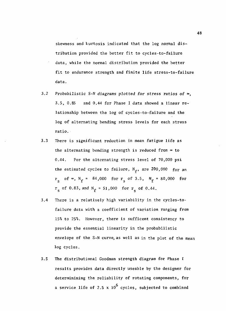
48

skewness and kurtosis indicated that the log normal dis-

tribution provided the better fit to cycles-to-failure

data, while the normal distribution provided the better

fit to endurance strength and finite life stress-to-failure

data.

3.2 Probabilistic S-N diagrams plotted for stress ratios of °°,

3.5, 0.83 and 0.44 for Phase I data showed a linear re-

lationship between the log of cycles-to-failure and the

log of alternating bending stress levels for each stress

ratio.

3.3 There is significant reduction in mean fatigue life as

the alternating bending strength is reduced from °° to

0.44. For the alternating stress level of 70,000 psi

the estimated cycles to failure, N_, are 200,000 for an

r of », N = 84,000 for r of 3.5, N = 80,000 for

r of 0.83, and N = 51,000 for r of 0.44.o -L o

3.4 There is a relatively high variability in the cycles-to-

failure data with a coefficient of variation ranging from

15% to 25%. However, there is sufficent consistency to

provide the essential linearity in the probabilistic

envelope of the S-N curve, as well as in the plot of the mean

log cycles.

3.5 The distributional Goodman strength diagram for Phase I

results provides data directly useable by the designer for

determinining the reliability of rotating components, for

a service life of 2.5 x 10 cycles, subjected to combined

49

alternating bending stress and constant shear stress at

various stress ratios for the given material and geometry

of the specimen tested.

4. Phase II of the experimental fatigue research program was

initiated and completed for specimens of identical specifications

to the Phase I specimens, except for a different groove radius to

provide a theoretical stress concentration factor of 2.34.

Fatigue tests were accomplished for plotting S-N diagrams for the

stress ratios of ~, 1.06, 0.40, 0.25 and 0.15.

5. The computer programs were revised to incorporate the current

calibration coefficients for the fatigue research machines, the

application of a revised Chi-Squared goodness-of-fit test, and a

subroutine for the plotting of a histogram and the estimated

normal, lognormal, and Weibull distributions using a Cal-Comp

plotter.

6. The conclusions reached from the results of the computer programs

are the following:

6.1 Increasing the sample size to 35 allowed the use of the

Chi-Squared goodness-of-fit test which proved to be more

discriminating than the Kolmogorov-Smirnov test. The

Chi-Squared test rejected the normal distribution three

times out of sixteen samples at the 0.05 level of signifi-

cance; whereas the lognormal distribution was rejected only

two times out of sixteen. Thus, the previous tenuous

preference for using the lognormal distribution for cycles-

to-failure data was strengthened. For the Chi-Squared test

50

to be valid, it must have five or more observations in each

cell; this requires that the end cells sometimes be combined.

The existing methodology describes the tails of distributions

with about 5% accuracy. A method to improve the accuracy

of describing the tails of distributions for use in calcu-

lating reliability is needed.

6.2 Comparison of the S-N and Goodman diagrams for Phase I and

Phase II research reveals that the endurance strength for

2.5 x 10 cycles of life and the finite fatigue life at a

specified alternating stress level are significantly

reduced when the stress concentration is increased by

reducing the groove radius. The S-N diagrams show that

the fatigue life for an alternating stress level of 80,000

psi decreases from 75,000 cycles for Phase 1 specimens to

9,000 cycles for Phase II specimens for a stress ratio of °°.

In Phase I tests, an alternating stress level of 50,000 psi

at the stress ratio of 0.44 approached the endurance level,

and a mean cycles to failure could not be determined. For

the Phase II tests at the stress ratio of 0.40, the 50,000

psi alternating stress level approached the highest stress

level that could be tested without suffering shear failures

during machine set up, and at this stress level the mean

cycles-to-failure was about 56,000 cycles.

6.3 The cycles-to-failure results emphasize the effect of stress

ratio on the fatigue life of specimens at specified levels

of alternating stress and the maximum stress levels at

51

which fatigue tests can be conducted. The upper limits for

the tests ranged from about 120,000 psi for alternating

bending stress for the stress ratio of •» to approximately

32,000 psi for the stress ratio of 0.15. Examination ofi

the S-N diagrams show that there is a limited useable range

for low stress ratios; consequently, the stress level and

stress ratio become very critical in a component design

using low stress ratios.

7. Generation and analysis of finite life distributional Goodman

diagrams reveal that the conventional deterministic Goodman diagram

is extremently conservative.

8. The FORTRAN Computer program to estimate the parameters of the

three-parameter Weibull distribution which would represent cycles-

to-failure data is providing good results. The program incorp-

orates the K-S and Chi-Squared goodness-of-fit tests. The K-S

test did not reject the Weibull in 17 tests, and the Chi- Squared

test rejected the Weibull 5 times in 17 tests. Based on these

test results, the Weibull can be considered a useable distribution

for cycles-to-failure distributions, although the lognormal is

favored by the Chi-Squared test.

9. Cumulative fatigue is a complicated and not completely understood

design area. Several theories have been developed with most

research devoted to understanding changes in material structure

due to microscopic crack nucleation and progression. Two methods

were investigated in this research for calculating the reliability

of a component sequentially subjected to a number of stress levels.

52

The method of equivalent reliabilities provides consistent

component reliabilities regardless of the order of application

of the different stress levels.

53

5. RECOMMENDATIONS

1. The Phase II type experimental research program should be

repeated for other geometries and materials, and a complete set

of S-N and Goodman diagrams should be prepared.

2. An analytical study should be made in search of a mathematical

relationship between infinite life and finite life Goodman

diagrams.

3. An analytical study should be made in search of a mathematical

model for the effect of varying stress concentrations and stress

ratios in fatigue tests.

4. Further study should be made of infinite and finite life Goodman

strength diagrams to determine (1) a more accurate model than

the ellipse and (2) if another failure theory, or combination of

theories, is more valid for fatigue failure than the distortion

energy theory.

5. A study should be made with sample sizes larger than 35 to

determine the effect of sample size on describing the tails of

the statistical distributions. As part of the study an error

analysis should be made comparing the predicted reliabilities

using the lognormal and Weibull distributions for the cycles to

failure data and for different sample sizes.

6. A Phase III experimental research program should be conducted

using ungrooved specimens so that the true effect of stress con-

centration on fatigue life may be better quantified comparatively.

54

7. An experimental cumulative fatigue research program should be

conducted by sequentially applying various levels of stresses for

specified numbers of cycles and to specimens with different

groove radii. The data thus obtained should be used to determine

the validity of the equivalent reliabilities cumulative fatigue

model.

55

ACKNOWLEDGEMENTS

The contributions of the following persons to the efforts of

this final report are gratefully acknowledged:

1. Mr. Vincent R. Lalli, NASA Project Manager

2. Messrs. Jim Blair, Michael Carrell, Scott Clemans,

Steve Cressey, Thomas Dodge, Everett Gardner, William

Guerrieri, John Kempert, Robert Mclaughlin, Roger Neill,

Wesley Shonerd, Anu Vaze, Robert Warner and Frank Watts

all from The University of Arizona.

56

REFERENCES

1. Mabie, H. H., and Gjesdahl, M. S.; "A Fatigue Testing Machine

for Reversed Bending and Steady Torque," Proc. SESA, XIV(1),

pp. 83-88, 1956.

2. Kececioglu, Dimitri B., Dr.; et al, "A Probabilistic Method of

Designing Specified Reliabilities into Mechanical Components

with Time Dependent Stress and Strength Distributions," The

University of Arizona, NASA CR-72836, 1967, 331 pp.

3. Kececioglu, Dimitri B., et al.; "Design and Development of and

Results from Combined Bending Torsion Fatigue Reliability

Research Machines," The University of Arizona, NASA CR-72838,

1969, 57 pp.

4. Kececioglu, Dimitri B., Dr.; and McConnell, J. B., "Calibration

of Combined Bending Torsion Fatigue Reliability Research

Machines and Reliability Data Reduction," The University of

Arizona, NASA CR-72839, 1969, 151 pp.

5. Kececioglu, Dimitri B., and Smith, J. L.; "Statistical Complex

Fatigue Data for AISI 4340 Steel and its Use in Design by

Reliability," The University of Arizona, NASA CR-72835, 1970,

175 pp.

6. Mood, A. M., and Dixon, W. K.; "A Method for Obtaining and

Analyzing Sensitivity Data," Journal of the American

Statistical Association, Vol. 43, 1948, pp. 109-126.

7. Spiegel, Murray R.; Theory and Problems of Statistics, Schaum

Publishing Co., 1961, 359 pp.

57

8. Fryer, H. C.; Concepts and Methods of Experimental Statistics,

Allyn and Bacon, Inc., Boston 1966, 602 pp.

9. Shigley, J. E.; Mechanical Engineering Design, McGraw-Hill Book

Comapny, New York, N.Y., 1963, 631 pp.

10. Kececioglu, D. B., Dr. and Guerrieri, W. W.; "Generation of

Finite Life Distributional Goodman Diagrams for Reliability

Prediction," The University of Arizona, NASA CR-120813, 1971,

240 pp.

11. Hahn, G. J.; and Shapiro, S. S.; Statistical Models in

Engineering, John Wiley and Sons, New York, N.Y., 1967, 355 pp.

12. Lochner, Robert H.; "When and How to Use The Weibull Distribution,"

Ninth Annual Reliability Engineering and Management Institute

Lecture Notes, The University of Arizona, November 1971, 45 pp.

13. Sturges, H. A., "The Choice of a Class Interval," Jl. American

Statistical Association, Vol. 21, 1926, pp. 65-66.

14. Osgood, Carl C.; Fatigue Design, John Wiley and Sons, Inc., New

York, N.Y., 1970, 523 pp.

15.' Miner, A. M.; "Cumulative Damage in Fatigue," Trans. ASME, Vol.

67, A 159, 1945, pp. 343-355.

16. Corten, H. T., and Dolan, T. J.; "Cumulative Fatigue Damage,"

International Conference of Fatigue of Metals, The Institute

of Mechanical Engineers and American Society of Mechanical

Engineers, London, England, November 1956, 14 pp.

17. "Simplified PRE-PDR Techniques for Assessing Components Reliability,"

NERVA, Aerojet Nuclear System Company, Reliability Calculations

for the Cases of Combined Stress and Fatigue Loading, 1970, 62 pp.

58

18. Sorensen, Arthur, Jr., "A General Theory of Fatigue Damage

Accumulation," Transactions ASME Winter Annual Meeting, New

York, December 1-5, 1968, pp. 420-434.

19. Serensen, S. V.; "Fatigue Damage Accumulation and Safety Factors

Under Random Variable Loading," presented at the International

Conference held in Warsaw, and published in the Conference

Proceedings, pp. 33-42, published under the conference title

"Fatigue Resistance of Materials and Metal Structural Parts,"

by The Macmillan Co., New York, 1964, 313 pp., Alfred Buch,

Editor.

59

FIGURES

60

rto

00c•r-t"O

0)CQ!HO

01CO

. . - f. 4J»-i <U ,~i 6 W C0) .* O rt -H 3•o o CQ (-< a> o

I-H rt u. S S0 H w.1 OQ (3 OCT3 <U

•H C C C,C fH r-l •!-! rt -H

</> O CU To oIS

Tt LO v£> 1- OO O> O,-H t-H •-( i-H I-H i-l <N

I/)1)

(UCO

6 a) ca 3 Ma e o TSVi -H in u T1

tfl U. U OO0) a) C tX 00 (X'H C CO C C/3 « -H -H X

Vi JD -H ^ rH 4-»O *H 'O -P P- P« fX.<U+j rt rt 10 -H -H 3 «4-io a j o < i ' i - | r - | O r t

g-t-lo

•ort0)4->toi00c

• HT)

g

<u c

<u rtC 6

•H

i-So ^o rt

<u<4-l Ulo o>

fn

O X• H 4->> -H

g-80)

O h• H I•P (1)

0)

O rt(/) M-l

00•HU.

61

bo iO .H -H rC

rQ rH CO fH CX-H

CO 3 4-1 Oo o> o c rt

U HH CO

t/>

3cr

rt

•Ptn

• H-o0)

130tr>

> -H(1> X

" 3T3 S0>

.5-5O <DO 10

<D

(1) -H•H •—(> -H

XI

O -i-t

CDO r-l

•1-1 I4-* d>

e oo0) -HX *->U rt

C/J 'W

U.

62

RS

Rt R4

(o) BENDING MOMENT STRAIN GAGES

ROTATINGSLIP RINGS

STATIONARY

HONEYWELL

AMPLIFIER8 RECORDER

(b) STRAIN GAGE BRIDGE ARRANGEMENT

Fig. Bending stress strain gage bridge.

63

'J

(0) TORSION STRAIN GAGE

SLIP RINGSROTATING

STATIONARY

HONEYWELL119AMPLIFIER8 RECORDER

(b) STRAIN GAGE BRIDGE ARRANGEMENT

Fig. 4 Shear stress strain gage bridge.

64

Cycles-to-fallure tests

Select bending stress level,stress ratio and assignresearch machine

Run PDP-8 computer program tocalculate visicorder outputdivisions

Select and install specimenin test machine, zero andcalibrate instrumentation

Apply pan weights and torquefor desired stresses

Run machine until specimen fails;record time-to-failure

Repeat until 35 specimensare run

Reduce and analyze the data

Stress-to-failure (staircase)tests

Select stress ratio, estimatebending stress level assignresearch machine

Run PDP-8 computer program tocalculate visicorder' divisionsfor a range of bending stresslevels

Select and install specimen intest machine, zero and calibrateinstrumentation

Apply pan weights and torquefor desired stresses

Run machine until specimen failsor runs for 2.5 x 10^ cycles(whichever occurs first)

Increment stress level up aftersuccess, or down after failureand repeat until 35 specimensare run

Reduce and analyze the data

Fig. 5 Flow chart of steps in cycles-to-failure and stress-to-failurefatigue tests.

65

s•

o

-N

aOO

ir\ro

ooo

(30

0)

•HO0)Cu(0

01V)

o(A

00•Hu.

0. DIA.KEY WAY

3/16 X 3/32

66

•^>—

N*.

63

" —» *—• — — — -|

3.00

6.00

63

' +AOOO-0-735^005

• DIA.

0.G3J ±0.001 RAD

Fi»> 7 Phase II research specimen geometry.

'RL9N3ULS 3DNVHnQN367

_oT

UJQ:ID_J

So

o

go>o

°o I.

O CV

O 6•H .H4-> Ocd a;^ O.

+-> oi/> o0> 00A

(0

•H O

S^X> LO•H tO

</>•H

0) VtH 4->3 w>

1— I•H O,ctf Tf<4H (OI J-O4-> I-HI W

O t-(X OCJ <«

00

00•Ho,

'HJLDN3H1S 3DNVHn<3N3 68

4-1 (/)O C

<Do 6•H -H4-> Ort 0)

0) O

s gir4-> O

<8w x§°-•H O

3 -^J3 LO

WO

0)(U 0)FH 4J3 WrH•H O

IO

</>

i-HO

00•HU,

'SS3H1S HVNIIAION

69

'H1DN3ULS 3DNVH(KIN3

I I

LO

(H I/)O C

<Uo B

CO V

in

0) 0)fn >

4-> g(/) OJ-l

•H O

V 0>fc +J3 tn

i—i•H o<+H tO

O4-> H-4I CO(/) I—I<D <

°o

00•Hu.

'SS3yiS "WMII/YON

70

oo•

o

O CID

O 6•H -rt+J OCO 0>to 0<

in(Ain T3(1) o>fc >4J Ov) o0 bo

0)ina)

•H O

in oi•H

<o a>f-l 4->3 in•-I•H Ort rf

OT

U ft

00•HU.

!Sd» ' HVNIWON

-HH+-H-H b|±H±l.:H±J-LH.I 1 1 L Ii i i MM ; i

ILLi. LTZTLi-LJJ-J ! i I LI

I ' I '.": i I i I

Li_i.J i U-4-1I TT i I T Tli j l

zrrrrrrti_UlLJltTljrrrrnjir

_i_L .L.1.M ' .' I

_!_.J.JJ_J..LU

-_,—,—1—l_J 1—i-^-

UlL]_i_LJ_L

1JI..J '_! I..!i L-L'-LLi" ' M M

71

I•HO

t-tVJ2

LO

O hH

<4H <D

O JC•H O,•Prt ,jFH 4-)

•HW S

LO

4-1 CJ

•a f-iO rH

43 0)4-> S

e o<u a:8 -o i^-h U

• Hrt C4J Oin -Ha) -H

5 "co

•a cofl> OC O

•H O

4-> I

O I

a) i—irt

T3 «r-\

JS <0 '4-> a> tn00 4-> CC tO <Da> E(H O -H

w to <o't &,

0) (/)O I-HC en TJCtf I-H 0)

3 O"O M OC O f-tW iw bO

00•HU.

UT ssaaas Suipusq 3uTq.Buaa^-[B

oII

I0)

o><+•!

O O6

c/> -H0) O

X </>O

T3O <DO >•H O

O

LO

O to<H

<J

n) 0)•H 0>•O 4->

O-H

C 3o w

•H 0>4-) (H3

43HH

'H <U•P OT

QO.

00•HU.

'SS3H1S 1VNIIAION

73

•w ^^

tp. <1>O I/)

0)o xprt J=h p

•Tsd>j ' UT ssajjs Suipuaq

LO

toI—I

(4-1o o>O CTj

74

COoHO>»O

CO

Co

CO«0

ooa

O

CJ

oCM

OvO in

00

toLO

g5U(Up.(O

S3

atH X!

I/) -H(/> 34)H «4-) O

U

•g*

!•C3 5

oV O

o •>f-t ^f

• H Ua)

</) O•H

V 4->x: -H

>% oxi u•o co"<U ^Dc o

1?x> wO I

01

4-> 0) (/)bO 4-> CC w <Ua) 6f-l O -H

Ul (Ua,VO i-tC W T3nj HH 4Jfc < >3 O

TJ f-i OC O M

UJ <4-t 00

00•Htu

oLO

UT

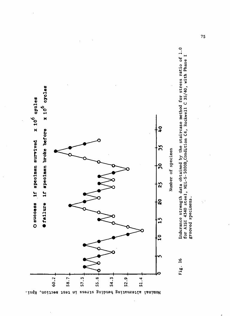
4-1O (U

O rt•H Xp a.cd

75

cov> 3O

£0

cov

UT ssaaas Sutpuaq

o•HO<Da*to

(4-1oH(I)

M toO to

^ U

P <0

i j*u4) Ow o:o •>f-> *t-

• H UrtP CI/) O

0) P

P -O

iS1i• H Ort m

2S

JS <0 •

M P CC (/) O53 e^ o -HP •«* oW to 0)

•* &.(u wu HHC C/5 T3rt M 0)fH < >

3 n §C O JHUJ ^H bO

00•Huu

•tsd)i 'UOTIOSS

9"76

3.75"

Section B Section A

(a) The length AB used for hardness measurements.

90° axis

(b) Test pattern for section A

Fig- 17 Grooved specimen sections used for hardness measurements.

0.75" 77

Legend:

C - center areaI - intermediate area0 - outside area 1/16" from surface

IA (a) Ungrooved specimen

r0.75"

(b) Grooved specimen

Fig. 18 Specimen sections and locations for hardness measurements.

78

§•

§•H4-1CISf-l

X)

01o4)

CO0>H

oo

•rl13gCQ

o>

00•Hu.

79

t<u(A

§•rl4->COH

COU

0)00

0)4SV)

g-HOE-

Oeg

00•rlU.

3.0

0.3150 DIA. ) For Phase I±0.0025 ) specimens

4.000 ± 0.010 RAD.

80

0.5000 DtA,

O.2.50O DIA.)For Phase II) specimens

Fig. 21 Ungrooved endurance strength specimen.

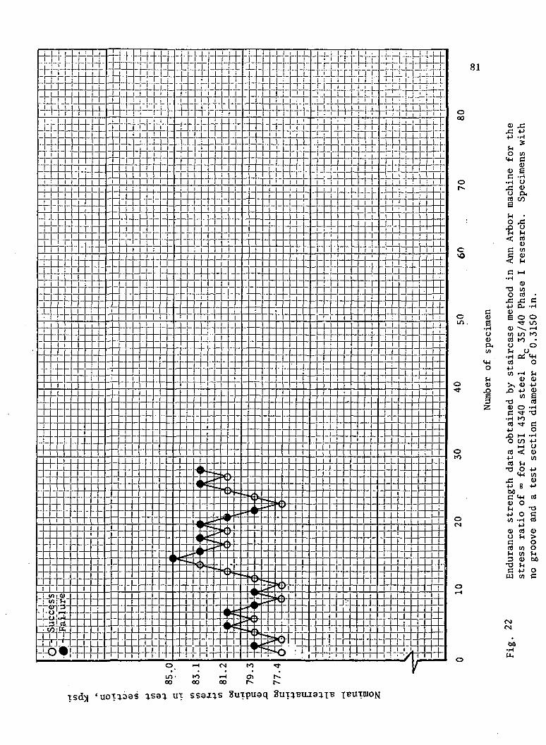
UT ssaxas Sutpueq

O (/>4-1 G

<UO £G -H•H G

O p<rt co6

oX)

rt(Uft(U

0>T3 </>O rt •x: x: c4-> a, -H0)S o o

• LO<1> ^ ^HCO LO tOrt too o!-l U

• H Oi 4-1rt O

0) OJX <U -P

^ w E•U rt<D O -HC ^^" ^3

•H (Ort rt- c4-> OXi I—I -i-lO CO 4J

l-l Grt <t 04-> I/)rt f-i

1 J p -LA

ooC <+-i rta> ot-i 134J O C(/> -H rt

4-J0) rt <DG f-t >

S Srt i/) O^H C/) ^H3 <U OO

"O HC 4-> OUJ to C

CMCM

00• H(JU

isd)j '

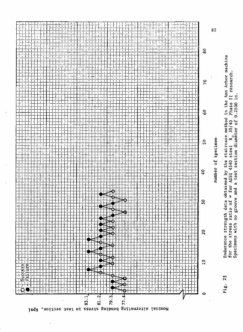
i i ' i i > i ; ;PITT i ;~TTT

TIXrE. i' J. J_l_l_!_i JI LIn niTT~

82

0)e•HO0)fXCO

0)

Iz

CDC•H

•scd

o^

ICD

c•H

COJ2 0> O4-> co O

cd LOe X CN•H 0. •

oo o tn.c •* o

g to o>4->

Ci> OCD10 o: eCd COO -Hh ^H T3•rl 0)rt cu C

to co -H

0) O Ox; ^ <u

toO)

cs o TJ+-> «+-i cO 8

0)

4-> O Oca o•o o ^

•H GO

•»-> rt oM (H C

<D CO XH CO ••->4-* Cl) >i-(10 ^ 3

4-10) CO COu cC CO 0)cd , £M 4-> -H3 O

T3 fn 0)C O P,

toesi

00•HPL,

isd)i 'uot^o9S

NORMflL DISTRIBUTION PflRRMETERS

0

83

CYCLES-TO-FRILURE X 10

MERN VflLUE:STflNORRO DEVIRTION:KOLMOGOROV-SMIRNOV TEST: 0.094CHI-SQUflREO TEST: 0.248SKEWNESS: -0.163KURTOSIS: 2.317

3297.1 CYCLES361.7 CYCLES

FIG. 24 CYCLES-TO-FfllLURE DISTRIBUTION OF |5GROOVED SPECIMENS FOR PIN RLTERNRTlfcSTRESS LEVEL OF108.900 PSI RT RSTRESS RRTIO OF INFINITY RNO NOMINRLGROOVE DIRMETER OF 0.491 INCHES.

LOG NORMRL DISTRIBUTION PRRRMETERS

00.

84

7.95 8.15CYCLES-TO-FRILURE

8-35

MERN VRLUE: 8.095 CYCLESSTRNORRD DEVIRTION: 0.112 CYCLESKOLMOGOROV-SMIRNOV TEST: 0.096CHI-SQURRED TEST: 2.844SKEWNESS: -0-374KURTOSIS: 2-408

FIG. 25 CYCLES-TO-FRILURE DISTRIBUTION OF 35GROOVED SPECIMENS FOR RN RLTERNRTINGSTRESS LEVEL OF108.900 PSI RT fiSTRESS RRTIO OF INFINITY RND NOMINRLGROOVE DIRMETER OF 0.491 INCHES.

85

'H1DNHH1S

p

o•H •4J Wd CM VsW -HV) O

w(0

o•u ^a 00w M§M

•H V+-> (03 rtjax:•H exM4-> Ow •^~•H^•O LOtooh o30i1-1•H Ort rt

<4H (Oi -<a-o

4-> I-Hi enio|-j(U <

1— IO, i-,

vO

00•HU.

'SS3M1S 9NIJ.VNd3.nv 1VNIWON

86

'H1DN3H1S 33NVynCIN3

oto

III III HIM I III I 11 I III I I M M I I II II I 1 1 1 1 I I I I I I I II II I

O ••H W4-» Crt 4)fn S

•Hv> o(0 <UO Pi

X O+J O

f-i4-> 00cti

i— iC HHo

3 rt^5 X•H a.M+J ow ^t

•HLO

(UO

•H Ort i^-

<4-t MI •^~o•»-> HHI O)

W HH0) <-(O !H

•Ha,oo

og oin

Oo

oa>

oID

O10

oCM

87

3DNVHndN3

P—- q

LJ

2

in

O

% oCT

°0 I.

O ••H V)4-> Ccd oh B

•HM UtO <U

ji o4-> O

&cd

i—i

H O

II•H (X

4-* ^3

0)

3 OS0

•H•H Ort •*4-i roi •*O4-> I-HI W

U) hH« <

°°

00•Ha,

3DNVynQN3

88

O vO Cvl OOtO CM CM rH

Q

-s

So

o

0

LOCM

O

0 ••H (/)

w otn a>w

•4-1 bflrtt—i

§ "•H 0>

3 rt•H cx•P o•H \T3 LO

M O3 oi

•H Ort ^-

(/> HHa) <r-l0 S-i>* O

bo

HVNIIAION

89

3DNVHflCIN3

\o

inro~

0) M

o o

_oT

"o ..p

•bo.

<D

fl-

LLJa:

§P

O

O

2enO

l/J

(4-1oo ••H l/l

rt CH PS

• H(O Ov> o>M w

0) >X! O•M O

H+-> 00oJ

•H 0)4-> V)3 rt& JS•H (XM4J O</> Tt

•H Ort ^>

O*J I-HI 05M h-l0) <

t>0•Ha.

'SS3yiS

J_iJ_U_.!_!_'I i i I I i I I f

!_!-.Ui.J_i_i! i fur i iI -JlL

i i M i ; !-LMjJJjJ

9)

OO

. . a

Q) <4-lW Ort

t-t riO »-c

4-((0

T3 t/)O C)

4-> •*->4) </)

0 O

O O

•H -~*.CS LO4-) tO

O<D ttC

XO)r> o>

<UC O•H •*rt to

O HH

rtJS•P <Crt

T34-Io

5bO

(Uf-l

<u v>O C

»-( -H3 O

T3 <UC ftU4 U)

DO•HU.

•Tsd)j 'uotaoas UT sssaas Suipusq

.UJ i U...LL

Li.L.U i I i iLLLfii ; , i i

._ | LL.i-1J J-LLJ

I ! ! I | I

- - H -J..J-.L.i_!.L

M I I i I i I i

! LI I I !i.! 1:"

LLLU-lI l i i i !

.LLLLJJJ-J..i j i i i ij i i i ' . :_v"r: r! i~i i r i . i 'F. ! i

91

(J0)Pi

o

0)

ID

O

2bO

(U</)a)

O. vOO

!H •O r-i

M-lM-(

•T3 OOX O

0)to tn03 c/>O 0)i 5n

•H 4->nJ </)

CMro

00•Hu.

'uoTjoas UT Sutpuaq

e•HO0PHI/I

&

O

rti£d

ooM-l

e aCDin incS </)O <l>

n) i/i

<fl fn

J3LOto

OS

O 4J

toto

00•Hu-

LJ.4-U .-UJ_U_l-Li-

nri.iJii.Lj.-L! ! j ! | j [ ! 1rr."TT~ri Tf

ILL-DILI!J i LL_J_L.iJ

1 !_U_L LLL1

1J_1_{ J J_1J i! ; i 1 i i Ii i • i rr i

U i l l !I i I i r' i | iI I I ! | I M

LO

93

to

LO

o(N

<uS

• HO0>

ID

(A

(US•HO0)ex

Sbo

(Art

cx

•5•HS

o

<uo(A

O O

•So, rt-H

(A(A

s s'cfl4J O

O ^-LO

Ctf (O

4-> 0)

c **O (A

(A rt-

O

rt W^ •-!

10

00•H

I I I ! I..!_!...!_j_

~rri~r

CM rg <N

UT SS8JJS SuTDUaq 3UT3.BUJC8aTB

<0e•Ho<u

M-lo

I

200

0)U)ri

O oM-i

^0 Oox o

tfl (/)oj i/iU 0)fn fn

•H +Jrt w

(fl ?-lo

0) <4-l

•(-> O

LO

oo• rtU.

oII

|H

\D

95

•HI/)CX,

CD10cd .a, o

toa>

<4-i a>

cdo 0V) CDo woX wo c

0)o 6o -H•-I O

oX CU

uiLO

CN 0)

£CO

00

to

J-ltoc

-o cdcxi a>

6i— icdC•^E

_o oVO Z

^

— oTt

.

h Oo o

t)_l ^t>0

cd O

bO .cd LO

•H tO

0X Pi4_>

bOC *^4) O(H 0)J j J 1

to toc ort •*S to•a roO HH

u toh^^ <

cdC ,CO +->•H •!-!j ^ S

*-v tft

•M 3(/) (/I

•H CUQ l-i

to

tsd)i 'ssaa^s 8uT5.BiU9q.jB

NEIBULL DISTRIBUTION PRRflMETERS

0

96

X 10

KOLMOGOROV-SMIRNOV TEST: 0.217CHI-SQURRED TEST: 4.236WEIBULL SLOPE (BETfl): 3-853MINIMUM LIFE (GflMMfl): 1999SCRLE PRRRMETER (ETfl): 1306

FIG. 37 CYCLES-TO-FAILURE DISTRIBUTION OF 35 GROOVED

SPECIMENS FOR AN ALTERNATING STRESS LEVEL OF

108,900 PSI AT A STRESS RATIO OF INFINITY"

AND NOMINAL GROOVES DIAMETER OF 0.491 INCHES.

97

TABLES

98

Table 1 Summary of nominal stresses applied to eighteenPhase I specimens for a nominal S = 65,000 psiand r e 0.44. a

s

Bending Stress (psi) , o = Sxa a

Shear Stress (psi) , Txym

Sa

Stress Ratio - • - — -•••

/7 T0 xym

Mean

64,700

84,900

0.44

Standard deviation

1,300

1,800

0.01

Table 2 Estimates for cycles-to-failure distributionparameters for S = 65,000 psi and r = 0 . 4 4 .

a s

Distribution

Mean Cycles -to-Fai lure

Standard Deviation

Skewness

Kurtosis

K-S Test Maximum D Value

Allowable D Value at the0.05 significance level

Normal

83,700

26,350

0.315

2.408

0.066

0.294

Lognormale

11.278

0.374

1.091

3.747

0.114

0.294

.8o130)

<u

IexC ••H (fl

in o>4-* &10 *H0) O

ft9) in3 T3

i—t iu•H >cd o

<4-l OI FHO 004-iI Oin • -

rH LOO to

r<o «

<4-l rH0)

m o>rH 4->0) (A>4) OrH ^

toin0) rHrH CO

CO <

tO

1)i-H

r?

e *to

in *U -Hin en3) ' ft

rH ^1 '"rj

Cd 4-> 4->C I/I CO

1 §

rH *cd c -H6 cd in

1 i ftc

*X >X <D

H T3 -H

rH * P|

cd w *OC m 4 - "

•H <U tO

Z w

cd c -Ho cd wr* 0) ft

cd *CO

l/l T3 -H

fH TJ ^

in co00

rH Ccd -Hc ~o•H C§£Zc°

cdC *

C -H

cd

rH CDft IM

to

(/) " Cin o cd0> -H 0)fH 4-> S

CO M

O 0 O O O

0 0 O 0 O

O O O O 0

0 0 O 0 0

0 0 O O 00 0 O O OLO CT* t~^ C7i GO

rH CM rH

o o o o oo o o o o

rH rH

CM 00 OO OO OO

8

o o o oo o o o•5f CM CN O

I— 1 I— 1 rH r— 1

o o o o0 0 O OrH t OO LO

IO tO tO rH

•"3- tO CM <N

o o o o0 O O O00 1* ^^ \O

o o o oo o o oCO (O t^ Tt

^ C7> tO CMCM rH i— 1 rH

o o o oO O 0 OOO OO CM OO* * *

tO rH i— 1

o o o o0 0 0 OO \O CM CM

rH Tt tO *3-LO rH 00 1i-H rH

CM OO OO OO

LO

to

0 O O 0o o o ovO t~~ O> to

tO VO LO CM

o o o oO 0 O 0rH O CM CM

1 LO tO rHCM rH O. OOrH i-H

0 0 0 Oo o o orH LO ^ tO

* * * * *CM tO tO rH

O 0 O Oo o o oto to r- oo* * * *

tO vO to \Of***. ^Q |_^ f

O O O 0o o o otO t-~ OJ Oi

rH \D to to

o o o oo o o oCM LO f~ CM

rH rH LO LOrH £7), ( . \Q1— 1

CM OO 00 00

tooo

o

0 O Oo o o

rH IO CM

o o o0 O 0\O to 00* * *

LO t"» LOLO '3- torH rH r-H

o o oO 0 000 00 '3-

* *i-H rH

0 O Oo o ooo o ^tCTl LO 0000 00 1 .

o o oo o o•^- to f-* *

rH I-H

O 0 Oo o oC7> t~- vO

OO 1" C7i\O vO LO

oo oo oo

o

99

o<u

t-t

CO<4H

O

<o

O

0)

oo•HI/)3

•H X</> . HftV0

O llOo S.i-H

II

C

O4-1

4-1

OX

V

II

TJ I to<U ^v

T3C

OS C0~

* *

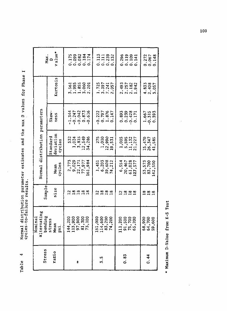
100

10rt

ex

in<D

i— Irt

Xa)

T3

rt

0)+->rie

•H•M

rH rHcfl 3OH (/)

CDC MO

•H CD4-> P3 3

•H -HrH OS

(/) I•H O

Cti CDE rHC OO X2 O

OI—I

•9E-

c3

inCD

rt

rtOn

(JO•H

• H

4->

•rtTJ

i-l

f_|

O

(UrHpre

CO

crH -H W

rt 4J cC rt -H•H C 'Oe rH CO CD U2 «•* .Q

rH

10to0)

4->CO

*0)< 3) O rH

rei

10•Hino4-1

3

i% tOCD (0

CO C

CT3 OrH -H (/)rt 4-> CD

T3 rt i— iC -H Ort > X4-> CD UCO T>

V)

§ rHCD US X

U

0)H N

I/)

>(0

CD C8 S.H.4-» 0> (/)t/> S 'P-

o•H

rtM

LO O> CN Tt Ttr 01 oo oo r*«rH O O rH rH

O O O O O

rH LO LO O rH

VO C7» LO VO OLO CJ) 00 O CN

tO rH rH tO CN

Tt t^ CN tO VOTt Tt Tt ^> rH

to CN o oo \orH O O O OI I I 1

CN Tt LO Ol VOtO CN rH Tt 00LO O OO LO CN

rH tO CN TtrH tO

tO Ol *""* ^^ Ttr^ CN t t~» oof« O rH CTl Ol

CN Ol CN r*. rHCN t>» vO

rH

CN OO OO OO 00

O O O O O0 0 O O 0

Tt tO f- rH tOTt rH Ol OO 1 *i— 1 rH

8

tO rH O> CNrH rH tO tOrH rH CN rH

O 0 O 0

LO r>» rH r~-CN Ol Tt LOt^ to CN orH tO t"- CN

CN r>» \o t~-CN 01 r TtCN t~- 00 rH

O O rH O1

LO O O rH1 rH Ol tOCN O Ol LO

rH CN OlrH rH

rH tO 00 CNLO 0 O rH

Tt CN VO CN

rH VO Ol Ttto Is*

CN OO 00 OO

0000o o o oO \O CN CN

LO rH 00 t--rH rH

LO

to

VO Ol Ol rHOl rH ^3 TtCM rH rH rH

O O O O

to r~ CN CN01 LO oo TtTt CN rH Ol

CN CN CN rH

tO Ol OO rH

01 to CN r»OO CN Tt rH

0 0 0 O1

LO LO CN f-O Ol tO CNO LO rH CN

rH LO rH rHrH CN

Tt t^ OO ^^LO \O CN tLO Tt O LO

VO O rH t-,CN vO Ol

i— 1

CN OO OO 00

0000O 0 O 0<N LO 1 CN

rH rH LO LO

rH

to00

o

CN t- OOf- VO TtCN O rH

0 O O

to oo r~to o LOOO Tt O

Tt CN tO

t-» LO tOVO rH OlvO to tO

rH O O1

O t-* LOt Tt OOTt tO LO

LO \O rHrH CN Tt

to o oIs* O LOLO r LO

to to CNLO 00 Tt

rH

00 00 00

0 O 0o o oOl I*» \O

oo Tt 01vO vO LO

Tt

m

0

COI

§

CO

101

to0)

rHrt

•Q

X

s-d

u

rt

•H

tot/)±JrH

»

r-lrt

rtrt

00 rHO O

<-! <4H

LO

•8H

9ss

V)fH(D4-><D

fHrtrt,co•H4_>3o•H

4-1tO•H

rHrt

RO

boo-4

(1)r—p

to

00c

rH -H brt 4-> CC rt -H

O O d>Z P ,0

(A10(V(H•pto

*_3

•>

•H

O•p

13 <o0) to

to c

CT) 0r-l -rHrt P <D

T3 rt bo

OJ > — I4-j d}tO T3

C <Drt bO

S <-<

0)H M

3to

M rt .H^J 0 £/)

o•H+jrtW

tv CN rr en ooO O O) LO OCN O O r-l rH

0 0 O 0 O

oo to LO r*> t"»LO CN ^ O» O

** CN rH CN CN

vO t~~ LO LO VOOO O VO t^ OLO •* CN LO C31

t-H 0 0 0 0I I I 1

OO vO vO " LOCN I-H r-» LO toCN rH i-H i-H CN

o o o o o

o o o^ LO r«»

1 C7V G^ rH rH

CN 00 00 00 00

O 0 0 0 0o o o o oCN Ol CT> tO O

Tf tO h^ rH tOT^ »-H o^ oo r*-rH 1— 1

8

00 ^D ^^ fCM OO 00 OOi-H O rH O

o o o o

O vO O OO OO ^ LO

CN CN f CN

LO to vO CNto o oo ^j-^t TT vO to

o o o o1 1

oo t r^ n-O) LO OO !•*•rH rH CN CN

o o o o

tO rH LO OvO CN ^ OOCN t~~ LO <-H

t*» OO O rH

CN 00 00 00

0 O 0 0o o o oO vO CN CN

rH ^t tO TttO rH OO fi-H rH

LO.

to

O O rH t^OO CN rH TTCN rH i— 1 i— 1

O O O O

Ol rH LO VOCN CTk •* t*>

CN i-l CN rH

CN rH (O O•^t f~N O tO!*• rH f^ O

O O O O1 1

VO rH LO CV^f 00 O vOrH CN rH rH

O O O O

OO O CN tOI""** ^3^ ^^ ^^^* oo ^^ r***

00 O rH rH

CN OO 00 00

O O 0 OO O 0 0CN LO t>» CN

i-H i-H LO LOi-H Oi f VOf— 1

to00.

o

rj- LO 00rH rH i-HCN rH i-H

0 O 0

cn r» CNOi t 0000 f~ rH

to to to

O rH f^<-H O» LOCN O 1 -

rH rH O1 1

OO Tf LO•<fr t^ OCN tO tO

O O O

i»- r-- LOLO 1 CNOO CN OO

O rH i-H

OO OO OO

0 0 Oo o oOJ ^^ vO

OO ** O>\O vO LO

'9-rj-

•O

(A(U

EOrH

rt

Ia

§

S

*

102

Table 6 Endurance strength calculations for the stress ratio of0. 45 using the staircase method at 2.5 x 10^ cyclesfor AISI 4340 steel RC 35/40 Phase I grooved specimens.

Nominalalternatingstresspsi

51,870

49,460

47,050

44,640

i

3

2

1

0

n.

Successes

3

7

5

3

N = 18

in.

9

14

5

. 0

As 28

i\

27

28

5

0 .

B =60

d = stress increment = 2,410 psi

X = lowest stress level = 44,640 psi0

X = mean (estimate)

Y = X + d[A/N + 1/2] = 44,638 + 2,411 [_ ° .X=49,597 psi * 49,600* psi

s = stcndard deviation' (estimate)

s = 1.620 d[(NB-A2)/N2 + 0.029] =- 1.260 (2,411) [18(60) - (28)

s = 3,681 psi s 3,700* psi (18)2

+ I]18 2

0.029]

Rounded off to nearest 100 psi.

Table 7 . Endurance strength calculations for the stress ratioof « using the staircase method at 2.5 x 106 cyclesfor AISI 4340 steel R 35/40 Phase I groovedspecimens.

103

Alternatingstresspsi

61,857

58,543

55,229

51,915

'

3

2

1

0

n.

Successes

1

2

10

2

N =15

in.

3

4

10

0

A = 17

.2xn.

9

8

10

0

B - 27

d = stress increment = 3,314

X = lowest stress level =51,915

X = mean (estimate)

"X = X + d[A/N + 1/2] =.51,915 + 3,314 [ IZ + 1 ]

X" = 57,317 psi 2 57,300* psi 15 2

s = standard deviation'(estimate)

S = 1.620 d [ (NB-A 2 ) /N 2 + 0.029] *= 1.620 (3,314) f 15(27) - (17)2 1

s = 2,924 psi s 2,900* psi (15)

* Rounded off to nearest 100 psi.

104

Table 8 Endurance strength calculations for the stress ratioof 3.5 using the staircase method at 2.5 x 106 cyclesfor AISI 4340 steel Rc 35/40 Phase I groovedspecimens.

Alternatingstresspsi

57,103

53,759

50,415

47,071

i

3

2

1

0

n.

Successes

4

9

4

1

N = 18

in.

12

18

4

0

A = 34

A36 '

36

4

0

B = 76

d = stress increment = 3,344 psi

X = lowest stress level = 47,071 psi_pX = mean (estimate)

X = XQ + d[A/N + 1/2] = 47,071 + 3,344 [ I ]

"X* 55, 059 psi =. 55,100* psi

s = standard deviation' (estimate)

S = 1.620 d[(NB-A2)/M2 + 0.029] = 1.620 (3,344) [ 18(76) - (34)

s = 3,701 psi H 3,700* psi (18)20-029]

-.* Rounded off to nearest 100 psi.

105

Table 9 Endurance strength calculations for the stress ratioof 1.0 using the staircase method at 2.5 x 10^ cyclesfor AISI 4340 steel Rc 35/40 Phase I groovedspecimens.

Alternatingstresspsi

60,168

58,707

57,246

55,785

54,324

52,863

i

5

4

3

2

1

0

n.

Failures

12

6

6

2

1

N = 18

in.i

5

8

18

12

2

o

A = 45

.2in.i

25

32

54

24

2

0

B = 137

d = stress increment = 1,461 psi

X = lowest stress level = 52,863 psi

X = mean (estimate)X = XQ + d[A/N - 1/2] = 52,863 + 1,461 [ li - I ]

X" = 55, 785 psi * 55,800* psi

s = standard deviation (estimate)

s = 1.620 d[(NB-A)

5=3,290 psi 5 3,300* psi

0.029] « 1.620 (1,461) [ 18(137) - (45)2 +

21.029]

(18)'

* Rounded off to nearest 100 psi.

•a

mino>fH•pin >

coT30) «C *

-H *£> *E fH0 00 4J

oi-H CDrt >c•Hso2

coE

•-(ca «s *fH *O inCif ivi

CD-1 fHfrt ij^\j +^C </)•HE CO OS2 1

0

nco

*,

tninCDfH*Jin

bO_j <-*

' ^Cfl -HC TJ•H fiS 0>O JO

00c•Hj t4^n)eo*J1— Icd

/A

*•>0>

T3 -HW

• OHT3+JCO

>Ico

*t«ccd -HCD inS OH

co6

b

*CD

13 -Hin

• OH"0X tT-*

co

eico

*S.HCD tnS OH

cdcob

*.>CD

T3 -Hin

• OHrO4-*CO

0)ico

M

*&H

<u inSO,

intn fnin ^d> ofH *i~(4J PCO n)

fH

O O OO O 0CT> o> r>-

*s *» •»CN tO Tt

O O Oo o ot*5 tO O>

•t «\ nr*. tv. ooLO LO t -

0 00 O

O i-l to•X *

•-I to

0 00 0

0 1 ^ . 0 0•s *i

LO VOi-H LO

0 0 0O O OW l-v tO

•\ -1 «CN tO tO

0 O Oo o oto i-H 00

•» •, *r» LO LOLO LO LO

LO O

8 to •-(

o0o

«\

o>

oo0>

•\

oCN1— (

0oCM

A00

ooCM

*»

o.-!1— 1

oor •ito

oovO

o>rr

LO•5J-

o

106

i-n| inhn

•HinCuoo

in

a)<uC

TJ , BJ<u IM"OC I

<§ l«

a)CO

to

COO

COD

a)

>Til"

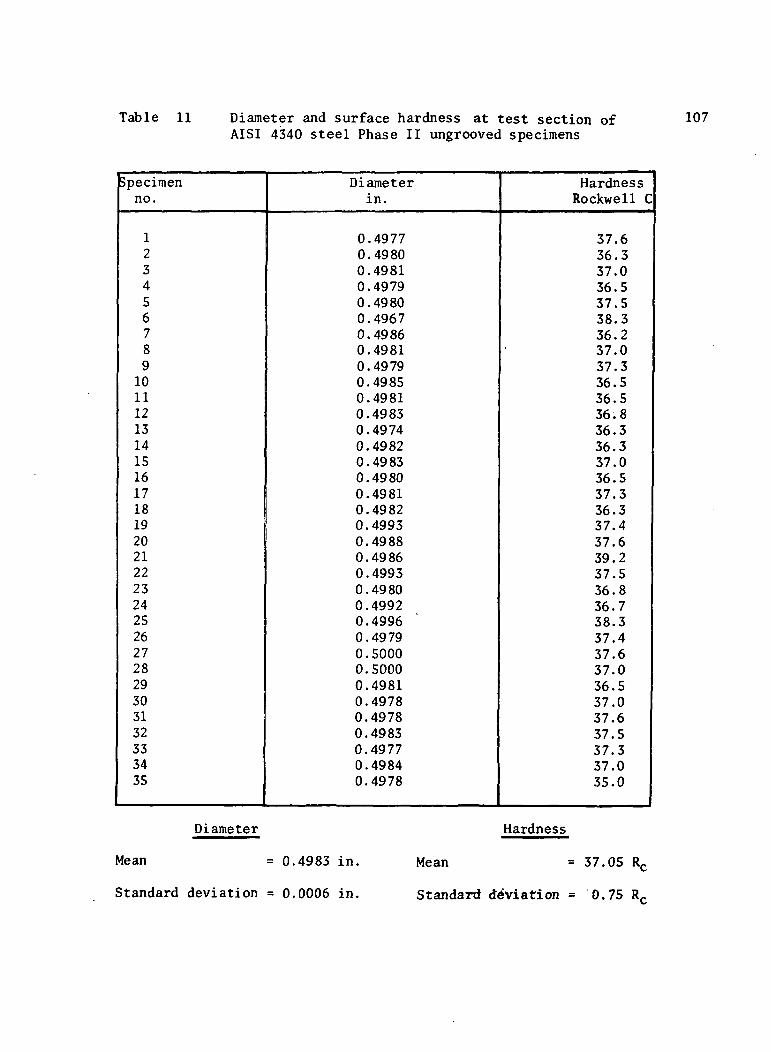
Table 11 Diameter and surface hardness at test section ofAISI 4340 steel Phase II ungrooved specimens

107

Specimenno.

123456789

1011121314151617181920212223242526272829303132333435

Diameterin.

0.49770.49800.49810.49790.49800.49670.49860.49810.49790.49850.49810.49830.49740.49820.49830.49800.49810.49820.49930.49880.49860 . 49930.49800.49920.49960.49790.50000.50000.49810.49780.49780.49830.49770.49840.4978

HardnessRockwell C

37.636.337.036.537.538.336.237.037.336.536.536.836.336.337.036.537.336.337.437.639.237.536.836.738.337.437.637.036.537.037.637.537.337.035.0

Diameter

Mean = 0.4983 in.

Standard deviation = 0.0006 in.

Hardness

Mean = 37.05 Rr

Standard deviation = 0.75 RC

Table 12 Diameter at the base of groove, groove radius,and surface hardness of AISI 4340 steelPhase II grooved specimens.

108

Specimenno.

1234567891011121314151617181920212223242526272829303132333435

Diameterin.

0.49280.49260.49090.49220.49530.49660.49660.49810.49360.49370.49720.49380.49470.49350.49730.49430.49070.49480.49520.49410.49690.49400.49380.49300.49340.49310.49370.49500.49340.49240.49320.49270.49390.49450.4933

Radiusin.

0.350.350.350.350.350.350.350.350.350.350.350.350.350.350.350.350.350.350.350.350.350.350.350.350.350.350.350.350.350.350.350.350.350.350.35

Surface hardnessRockwell C

38.137.637.638.137.337.536.337.638.037.437.536.637.637.536.537.137.237.437.537.038.336.537.537.337.438.036.337.337.237.036.538.136.937.837.0

Diameter

Mean = 0.4939 in.

Standard deviation = 0.0021 in.

Hardness

Mean = 37.29 Rr

Standard deviation * 0.53 Rr

Table 13 Hardness measurements at Section A of Phase IIgrooved specimens in RC units see Fig. 17 for locations.

SpecimenNo.

33

34

35

1

36363736

X = 36

T = 36

35373436

X = 36

f = 36

)T =X =

.0

.5

.0

.0

.4

.8 Rc

.0

.0

.0

.0

.5

.9 Rc

2

34.536.035.536.0

35.5

36.4 Rc

37.036.536.037.0

36.7

35.037.535.535.5

35.9

3

36.536.035.536.5

36.2

36.536.536.537.5

36.8

37.037.036.537.5

37.0

Location

4

36.537.036.037.5

36.8

37.536.037.038.0

37.2

38.038.037.538.0

37.9

No.

5

37.037.037.037.0

37.0

37.536.537.038.0

37.3

37.037.537.037.0

37.1

6

36.537.036.536.0

36.5

37.536.537.037.5

37.2

37. S37.536.037.0

37.0

7

36.536.536.037.0

36.5

37.036.036.537.0

36.7

37.038.036.536.5

37.0

8

36.534.536.536.5

36.0

37.537.036.036.5

36.9

Axis

0°0090°900

000090°900

0°0090090°

Table 14 Hardness measurements for Phase II specimens atSection A shown in Fig. 18 in R unitsc

110

Ungrooved Specimens

Specimenno.

31

33

34

R units

C = 36.5 36.5 37.0

I = 36.0 36.0 35.0

0 = 34.5 35.0 36.5

C = 37.5 38.0 38.0

I = 37.0 38.0 37.5

0 = 36.5 36.0 35.0

C = 33.5 35.5 34.5

I = 37.0 36.0 37.0

0 = 35.5 35.0 36.0

X

36.7

35.7

35.3

37.8

37.5

36.0

34.5

36.5

35.5

T

35.9

37.1

35.5

Grooved Specimens

Specimenno.

33

34

35

R unitsc

C = 36.5 37.5 37.0

I ~ 36.0 38.0 37.0

0 = 36.0 36.0 36.0

C = 35.0 36.5 36.0

I = 36.0 35.0 36.0

0 = 37.0 35.0 35.0

C = 37.0 37.5 37.0

I = 35.5 37.0 36.0

0 = 35.0 35.5 35.0

X

37.0

37.0

36.0

36.0

35.7

35.7

37.2

36.2

35.2

X

36.7

35.8

36.2

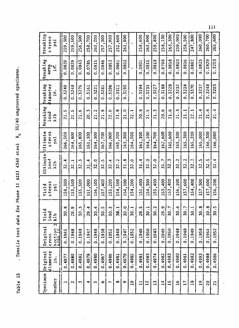
Ill

ca>• HOa>n,

OOrH00

LOto

o•=!•to

rHo

Cfl4->CO

•Htnc

t£c </>•H V) TI4*t o virt M O,<D 4J

£ «be

5 g*f*scc

M fnC <0

•H. 4-> •^ (U -C

CtS £ •»"•*a) ojfH -rl

OC

• H *O^ OJ J3rt O •-<<U r-i ^

CC

o> tn4-> V)« O -HE T»l w

•H 4-> CX«-" t/>

^O4-»« T:E r*« _T>•H O "-I4-) rH r*-H

1

tf>•O in •!-<

e> fn a•H 4-»>* I/)

rS-O0> ri .O

•rH O i— <>- rH ,*

CMi-Hrt ccC C-r-•H v; -Hbl If. 4J C

•H o oc;»H JH c.«-

O- O w a

r-l rHcs <i>C 4-> •• H O C« e -.H•H CStH -H ,O T3 !

Spe

cim

en

num

ber

1

ootocnLOCM

CnCN00oo

cn•<tCN«oo

ini— <CM

O0LO

VOvO

•*!•

CNto

OotoooLO

oo

0to

LO•sren

o

t-^r»Cn

°

i— i

lo0LO

CnLOCN

CnCN00oo

00^tCNto0

LO

1— 1(N

oo00

•<*vO

rH

CMto

OOLO

COLO

cno>cs

oo<3-0>

0

oooOk

0

CN

ootovOLO(N

to•*J-00o0

\0t~~(M

to0

vO

rH

(N

ooooLOv£>

to(N10

0OLO

LO

LO

tooto

00•t0>

o

I— 1ooo

0

to

oor>-00LO(N

LO00r~0

o

iHvOr-t

to0

to0CM

ootor— (vO

•<*1— 1to

o0oI— (LO

•<3-

O>CM

r~-• ra>

o

o>r^o>

o

•*

0oCS!

0\oCM

LO.-100oo

r-tCMCNtoo

CM

i-HCM

O0to• ~vD

O

CMto

Oor-l

vOLO

•<*O10

00•<to>

o

o00o»

o

LO

ootor~LOCM

vOTj-00oo

rH00CMto0

00

r-lCM

00t-~t-~\o

LO

CMto

0oTJ-r-LO

LO

OK)

00toO)

o

r--\oo>

o

vD

0Oa>iLOCM

toLO000

0

vOo>CMto0

oCMCM

0oovOvO

• fCMto

0oCM

LOLO

tooto

CMLOo

0

vO00o>

o

t~-

00\D

CMLOCM

f— 1vO00oo

f— 1r-ttotoo

00

rHCM

ooCM

LOvO

CM

CMto

o0LO

• J-LO

1— 1

0to

a>•51-o>

0

1— 1ooOl

o

oo

0oa>rHVDCM

CM000O

O

LO

o»rHto0

orHCM

00toto\o

00

rH

to

oorH

•<3-LO

0

oto

t-^• >0)

o

o\t~~en

o

o>

1

rH

CMCM

0o0

TJ-\D

oCMto

o0CM

Tj-LO

rH

0to

CMLO0>

o

LO00at

o

0rH

o0vO

enLOCM

rHo00oo

Tl-0»1— 1too

oo

oCM

o0r-H

rHV0

•<±rH

to

ooT±rHLO

LO

ChCM

o»Tten

o

rH00en

o

rHrH

0oentovDCM

LOrH

000

o

rHtoCMtoo

LO

1— ICM

oorH

"*\D

oCNto

0otor

LO

rH

oto

oLOen

0

to00en

o

CMrH

OO00

cnLO<M

00r-t00oo

1-CMCMtoO

torHCM

O0r-~-TVD

0

CNto

O0•<3-

LO

LO

CM

Oto

torrcn

0

•*r^cn

o

torH

OO

rH

00LOCM

00cnr^oo

0000rHtoo

vO

oCM

e>ovO

CMvO

t^1— 1to

0oTfrtoLO

cncnCM

cnTtcn

o

CMoocn

o

nrrH

O0totovOCM

00rH000

O

00CMCMtoO

vO

rHCM

OovO

LOvO

toCMto

o0• ~CMLO

I---oto

0LOcn

o

tooocn

o

LOrH

0

00

cnLOCM

0fN000

O

CMtoCMtoo

torHCM

00toLO

vO

CN

CNto

0orH

vOLO

**oto

oo•*t-cn

o

0oocn

o

vOrH

O0LO

00LOCM

vOi— (000

o

^fCNCMtoO

rH

rHCM

OotoLO

vO

CN

CNto

oovO

r^LO

r~oto

cn•<rcn

o

rH00en

o

t-^rH

O000

t--^t

CN

CNcnoooo

or~totoo

rH

CNCM

o0CM

LOvO

CN

CMto

0o•*!•1 -LO

rH

Oto

cn• ~cn

o

CM00cn

o

00rH

OOO

OvOCM

toCM000

0

t^toCMtoo

•o-rHCM

OooLOvO

LO

CNto

ootor-.LO

00

oto

00LOcn

o

!

tocncn

o

cnrH

OO

l~^

OvOCM

cn(M00oo

00TTCNtoo

vO

i— 1CM

OOtovOvO

LO

CN10

0ovO

1-LO

00

o»o

TtLOcn

o

0000cn

o

0CM

0ovO

LOvOCN

tooCMtoo

to0CMto0

• ~rHCM

0o0

vOvO

• >

CNto

0oCM

vOLO

LO

Oto

CNLOcn

o

vOOO

*?

O

rHCN

4-1

Ou

tn<u

O<D

OOHOO

LOto

Ooi

0><u

oTl-to

0)vtrtafH

rtTJ

4-»

0)

toSH

LO

OI-H

.0c3

Bre

akin

gs

tre

ss

psi

M..5 & .,* o c

CO fH -r-i

v At-<es

M ^C 0>

•H 4-> •^ <U C

OS E -H0> ojfH -ri

C* FT*

M

•H T3.* ea ,0C3 O •-!<U ) ^

ec

o> in•>-> V)C3 0 -H£= 5-3 t/)•f-i *J ft+J (0

3

o4->rt T3F rt .0

•H Q i-H•W t-H ^1— (=3

I/IT5 Ift -H

<U N ft•H +J> r / \

*T3r-l 13Oi rt X)

•H O r-(>- »H X

CM

rt CCc c---•rH -S> -HS£ W 4-! C:•H c oa^ ^ <U>-O o in oj

-H Vi« <uC 4-> •• H O C« £ -H

•i-l TO!-• "t~l |

O T3 1

C*\

E ^•rt O0 £><U £c, -cn S

0o0

*,

t^LOCM

COLOOO0

O

LOOtotoo

I— 1

CMCM

0OLO

vO\o

vO

CMto

0otovOLO

vO

0to

OOLO01

o

to01

I 0

1 ^1°

CMCM

0ooCNJLOP>J

LOVOCOO

o

CTi1— 1toto0

CO

1— I<N

0oCO

LOvO

to(Nto

0ovO

v£>LO

LO

oto

CO•*Ol

0

000C7>•*3-

0

toCM

0o0

1LO(N

1toCOoo

TfrvO<NtoO

LO

t-H<N

O0LO

LOvO

• f

(Mto

OotovOLO

vO

oto

f~LO01

o

„m<3\^s-o

rj-CM

0oto

•\

0vO«N

• ti— 1COO

0

o(N(NtoO

fM

i— itN

O0toLOvO

•*<Nto

o01— 1

vOLO

vO

0to

0vOat

o

vOo>0»•*o

LO<N

0oOl

•V

tovO<N

COr-lOOo0

COCMCMto0

vO

1— 1CM

ooo>LOvO

toCMto

o0CM

t^LO

vO

0to

r^• ~0»

o

0^t^01• ~o

vOr>j

0oCO

LOLOCM

ovOCO0

0

010toto0

oCMCM

0oLO

vOvO

r~.CMto

0o01

vOLO

CO

0to

to\001

o

oooLO

o

I-.CM

F0oCM

•t

CMvOCM

0CMCO0

o

iHtoCMtoo

LO

i-H(N

O0oLOvO

•<*CMto

o0Ol

LOLO

vO

0to

to\O01

o

0o0LO

o

00CM

oovO

LOvOCM

toOOt^oo

COLO1— 1to0

OO

0CM

ooCM

^vO

oCMto

ooLO

•ttLO

I-l

oto

OlTl-Ol

0

i-HCO01

o

OlCM

0oi-H

ovOCM

vO01f^o0

to00F— 1

to0

r^

oCM

oo"fr

CMvO

vO

I-l10

oovO

CMLO

1OlCM

vOrrOl

o

00!Ol

o

oto

ooo>

#t

00LOCM

oI-(to00

0

CMLOCMto0

LO

r-lCM

0oLO

vOvO

•«3-

CMto

0o1vOLO

LO

oto

V0•*Ol

0

00t^Ol

0

1— 1to

ooOl

I— 1COCM

tovOr^oo

vO1— 1>— 1to

o

LO

r-4CM

o01— 1

vOvO

Tfr

CMto

o0TJ-

LOLO

to0to

oLOOl

o

toCOOl

o

CMto

0oLO

COLOCM

• t-CMCOo0

OltoCMtoo

to1-1CM

o0LO

vOvO

•<*CMto

0oCO

vOLO

LO

oto

LO• rOl

o

r~-l-~-Ol

o

toto

o0Ol*to

vOCM

vO00[0

o

•*vOi-Hto0

OO

oCM

0oLO

•*!•vO

I— I

CMto

0oOO

toLO

ooto

f— 1LOOl

0

**00Ol

0

{

Ttto

1

1

1

0o0

t^vO

LO

CMto

oo1vOLO

LO

oto

vO•<a-01

o

OOt^01

0

LOto

112

O<1)&in

o•H

03

V)

<4HO

to

13

'=

to

o o oo o o

</)| CO LO CM

i-T t-H 00

so o oo o oLO »H Ol

• » • * * »LO LO OLO vO vOi-H i-H CM

to

Q) W)+-> eCIS -H6 J*

•H Cfl+J O—I f-<r> CQ

Table 16 Elongation test data for Phase II AISI 4340steel Rc 35/40 ungrooved specimens .

113

Specimenno.

12345678910111213141516171819202122232425262728293031323334

Elongation2-in.

gage length, in.

2.3652.3622.3652.3802.3562.3572.3492.3682.3622.3572.3572.3602.3612.3612.3592.3532.3542.3472.3602.3612.3602.3472.3402.3602.3532.3612.3582.3652.3652.3612.3562.3562.3562.361

Elongation%

18.2518.1018.2519.0017.8017.8517.4518.4018.1017.8517.8518.0018.0518.0517.4517.6517.7017.3518.0018.0518.0017.3517.0018.0017.6518.0517.9018.2518.2518.0517.8017.8017.8018.05

Table 17 Tensile test data for AISI 4340 steel RC 35/40grooved specimens.

114

Specimennumber

1234567891011121314151617181920212223242526272829303132

Originaldiameterin.

0.49280.49260.49090.49220.49530.49660.49660.49810.49360.49370.49720.49380.49470.49350.49730.49430.49070.49480.49520.49410.49690.49400.49380.49300.49340.49310.49370.49500.49340.49240.49230.4927

Originalcross

sectionarea, in.

0.19060.19060.18920.19030.19270.19370.19370.19490.19130.19140.19420.19150.19220.19120.19420.19190.18910.19230.19260.19170.19390.19160.19140.19090.19120.19090.19140.19240.19120.19050.19040.1907

UltimateloadIb

52,50051,95051,75051,90052,20051,40051,30052,20052,00051,50052,30051,60052,00051,60051,90051,45051,30051,60052,10051,60052,50051,25051,15051,05051,80051,65050,90051,55051,50051,00049,60051,250

Ultimatestresspsi

275,400272,600273,500272,700270,900265,400264,800267,800271,800269,000269,300269,500270,600269,900267,300268,100271,300268,300270,500269,200270,800267,500267,200267,400270,900270,600265,900267,900269,400267,700260,500268,700

Summary of static strength resultsgrooved specimens.Ultimate strength

Mean = 269,000 psi

Standard deviation = 2,800 psi

Table 18 Summary of tensile strength parameters forPhase I and Phase II specimens.

115

Ungrooved

Yield

Mean

psi

Standard deviation

psi

Phase I

Phase II

171,000

155,500

2,800

1,800

Ultimate

Phase I

Phase II

177,900

165,100

2,600

1,500

Breaking

Phase I

Phase II

254,800

261,000

4,400

8,200

Grooved

Ultimate

Phase I

Phase II

255,300

269,100

2,700

2,800

116

Table 19 Calibration coefficients and speed for each researchmachine and for Mode 5 operation*.

Machineno.

1

2

3

KBGR

1.3081

1.3081

1.3081

KGR-TH

0.0149

0.0145

0.0170

KT

0.8753

0.8950

0.8748

KT/B

-0.0462

0.0463

0.0542

KB/T

0.0477

0.0555

0.0645

Machinespeedrpm

1779

1775

1778

*Mode 5 operation refers to the computer program code which identifiesthe proper calibration coefficients to be used with each set of machinedata obtained during a specific calendar period. Mode 5 calibrationcoefficients should be used for all data obtained after June 1, 1971 untilthe next calibration.

117

Table 20 Endurance strength distribution parameters calculationsfor 0.3150 in. Phase I research AISI 4340 steel Rc35/40 ungrooved specimens for stress ratio of °°.

Alternatingstresspsi

85,000

83,100

81,200

79,300

77,400

i

4

3

2

1

0

n.

Failures

1

5

3

4

0

N = 13

in.i

4

. 15

6

4

0

A= 29

.2i n.i

16

45

12

4

0

B = 77

d = stress increment = 1,900

X = lowest stress level = 77,400 psi_°X = mean (estimate)

X = XQ + d[A/N - 1/2] =, 77,400 + 1,900 [1£ . I ]

X" = 80,725psi 2 80,700* psi 13 2

s = standard deviation (estimate)

s = 1.620 d[(NB-A2)/:.'2 + 0.029] * 1.620 (1,900) [ 13(77) - (29)2

S = 3,040 psi 2 3,000* psi 2

0.029

* Rounded off to nearest 100 psi.

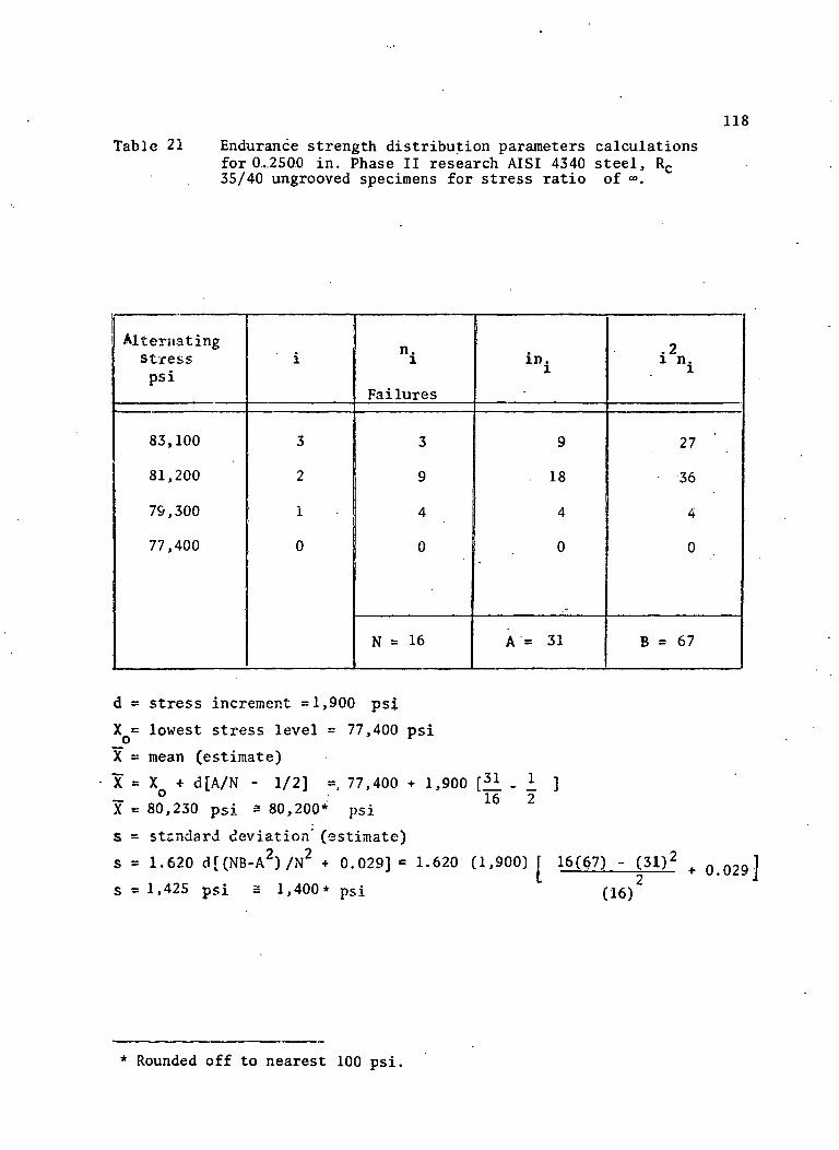
118

Table 21 Endurance strength distribution parameters calculationsfor0..25QO in. Phase II research AISI 4340 steel, Rc35/40 ungrooved specimens for stress ratio of °°.

Alternatingstresspsi

83,100

81,200

79,300

77,400

i

3

2

1

0

n.

Failures

3

9

4

0

N = 16

in.i

9

. 18

4

0

A= 31

.2i n.i

27

36

4

0

B = 67

d = stress increment =1,900 psi

X = lowest stress level = 77,400 psi_P f

X = mean (estimate)

X" = X + d[A/N - 1/2] =, 77,400 + 1,900 [H - I ]

X" = 80,230 psi 2 80,200* psi 16 2

S = standard deviation' (estimate)

S = 1.620 d[ (NB-A 2 ) /N 2 + 0.029] = 1.620 (1,900) \ 16(67) - (31)2

s = 1,425 psi = 1,400* psi (16) 20 029

* Rounded off to nearest 100 psi.

o(/)(U

I(X

c ••H in<n a>m -Ha> o4-> 0)

a> m

•H >rt o

<+-i oi t-t0 oo4->

1 Oin rr

i-H LOo to

9)<n a>

rt 4Jv co<D ofH 'S'

to

(O4) r-HfH CO4-> r-H00 <

CMCM

0)1—I

g

**eco

•*

(/)

(Uf-<

rt wC

O (U2 B

i— irt£oc

E

£*"

I-H inrt </>C 0)

• H f-t

O I/)2

rt0)X(fl

a

inin

woo

—i Crt -HC TJ•H CS 0>

Z w>C•H

rtg4-1rtrt

<l>2Prtf-t(1)><

.

>Vd -H

d'j-in

§5 'u>s a,

.s>d -H

dPo

3 -H

S OH

*>0)d -H

in

ir>

i•rt ,_iiU nD in

a, N6 -Hrt coW

in

t/> •>V) O<D -HI-l 4->4-1 rtCO OS

0 O O O O

o o o o o

o o o o o

o o o o o

0 0 0 0 Oo o o o oto t^ oo to ^r

^^

0 O 0 O 0o o o o o

00 CM tO O» CT»

1— I

LO LO LO LO LOto to to to to

8

0 O 0 Oo o o o• vO •f •*

1— (

o o o oO 0 O OO O O f-

Oi rt rt tO> 00 vO to

o o o oo o o oOO Tl- CM CM

o o o o0000• - t>. to oot^ \O LO fHLO rj- tO CM

0 O 0 O0 0 O OtO O LO CM

p^

0 o 0 0O o O O•"* CM CT> CM

LO LO "* 0O oo \£> *3-

LO LO LO LOto to to to

NOoI— 1

O 0 Oo o of 1* OO

CM rt

O 0 00 0 Ooo LO oto en r-CM O» 001— 1

o o oO O 0•^- o •^~rt i-H

000o o oLO LO tO

rt 1 . 0t LO LO

o o oO O 0CT> vO CM

O O 00 O Of- O fH

O> O LO^j- ^ to

LO LO LOto to to

o,

o

o oo o• j- eni-H i-H

o o0 O1 LO

o> oLO •*i-H i-H

o o0 000 rt

i-H

0 0o oCM rt

CM rt0> 00

o o0 0•* to

o o0 0vO O

O> LOto to

LO LOto to

LOCM

0

o o oo o o0 vO O

CM CM CM

o o o0 O O

to ^ toI-H oo rCM rt i-H

O 0 O0 0 OCM LO CM

i— 1 i-H i-H

o o oC3 C3 ^^c^ to to

tO \O OCM 0 0i-H i-H rt

o o oo o oLO 'S- to

o o oo o oo •* oCM f^ \OtO CM CM

f>- LO LOto to to

LOi-H.

o

119

oo

(DMrt<D

•80)

•O

O

X

oo6

•ort

oV

(1)

rt

I

I

bO

to

II

i-H

(/)CD

10OS

P-

rH

•810tHd>4->a)

XI

a>M3

i-H•Hn)

IHiO4->II/Ia>

i-HOXo

»w

8oz

toCN

CD

3of

•H

6

4J

a

U)i

:ai lu

re

oiVi-HO

u

otc•H

£04-1rH

lue *

****

rtD

egre

es

of

fre

ed

om

**Q *

. CDX 3rt rH

2 rt

•H

O4-J

3

inin0)

o>to

lard

itio

n***

C -Hrt >4J COto o

£

>

*into

rH tn

inrH

in o"O -HrH I *4-) rttO C£

OO I-H O CT> O•t LO 00 CN OCN i-H 00 vO Oi

O VO 0 rH *3-

rH CN CN rH rH

- ^1- 00 OO vOGt to O O rH

0 O 0 0 O

1^ CN "* CN OrH 1 LO CN 00tO VO VO OO rH

CN i-H CM CN tO

tO LO Is* to f

rH tO fr LO 1^

O O 0 0 O1 1 1

o o o o o\O i-H t 00 vOto vo to LO ^r

i-H tO VOrH

0 0 0 0 Oo o o o o

to vO ^f ^ vOi-H CM OO

O O O 0 OO O 0 0 0

OO CM tO O> O>co cji r** ^ toi-H

8

LO vO LO tovO CN O LOCN t*^ ^^ ^"

rH O rH CM

rH CN rH rH

CT> rH O> CNO rH tO rH

o o o o

vO [ LO to00 00 O> ••*!"•» rH O rH

CM CM tO tO

CN O t^ 010 o m LOCN CN r voO O O O

O O O OLO i-H VO OO

rH CN tO00

O O O 0O O O OLO OO to O

•<* o r •*rH CM CN

O O O Oo o o of~ CN CTl CN

LO LO f OO OO vO ^t

0

1— 1

(T, r-t COCN tO CNO vD C7)

tO O CN

rH i-H rH

• - tO rH

LO O O

o o o

\O "t OOCN vO tO\O tO rH

to to LO

CT> LO 00vO to f-

O O rH

o o ovO t-> vO

O> vO OtO rH

i-H

o o oO O 0o t^ iO> O CNLO rH tO

CN tO

0 0 0O 0 Ot* CD rH

CT> O LO• - *» to

0

o

vO vO0 OVO rH

CN to

rH CM

O 0)

rH O

o o

o oCN enCN r~CM CN

to t-oo 01tO LO

o o

O 0vO OlLO r• - CNi-H CN

0 0CN O

LO CT>

o o0 0vO O

O> LOto to

LOCN

o

3 !0

t-~ LO -Hi— 1 P~ rHO 00 4-> P,

i— 1 tO Z rt

rH rH O

10 vO *!•C7> O OlO rH rH

O O O

00 i-H O>LO 00 •*!•t~~ oo o

CN tO vO

vO OO OCN t~» vOLO LO LO

O O rH

o o oO vO 00OO LO •*

I-H r <oto vO LO

i-H

0 O Oo o oO i— 1 rH

00 CM f

i-H CN LO

0 0 00 O O•-H Tfr O

CM Is* vOtO CN CM

LOrH

o

120

••HU)OH

o0rH

4-*

10)oeo4-*

UH

o*o0)

13c3o&«

V)(O

•-Hu(_>

ooi-H

4->in

cdCDco^

ttjo*oco•oc30a:

*4e

tn0

i-Ho

orH

4JtnCOrHrtCD

o

0•o

1rH

co

rH•Hrt

o

inrH

0X0

<4Hoe0•H4Jrt•H

0)•o*orHrt•art4J

CO«4141

CNCM

o

• H

LOto<4H0

<Dtq•Htn

COrHPH

•a

CJ

so•H

•H

oi•Htn

(4Ho

rH

CO

0)rH

LOoo

rt

rtu

• H4_>• HrH0

a

*41

**

Chi-sq

uare

d te

st

at

0.0

5

level

of

sig

nific

ance

rHo

<4H

CO3i-Hrt

^^H

rt0

•H4^J•I-lrHu4-*ucocorH

4_)PwCOu0

4,

414i4t41

Critical

valu

e

e0

co<u«l

^M

MHoinCOCOrHbOCOQ

rH rH

"* O>00 O>

tO LO

i-H CN

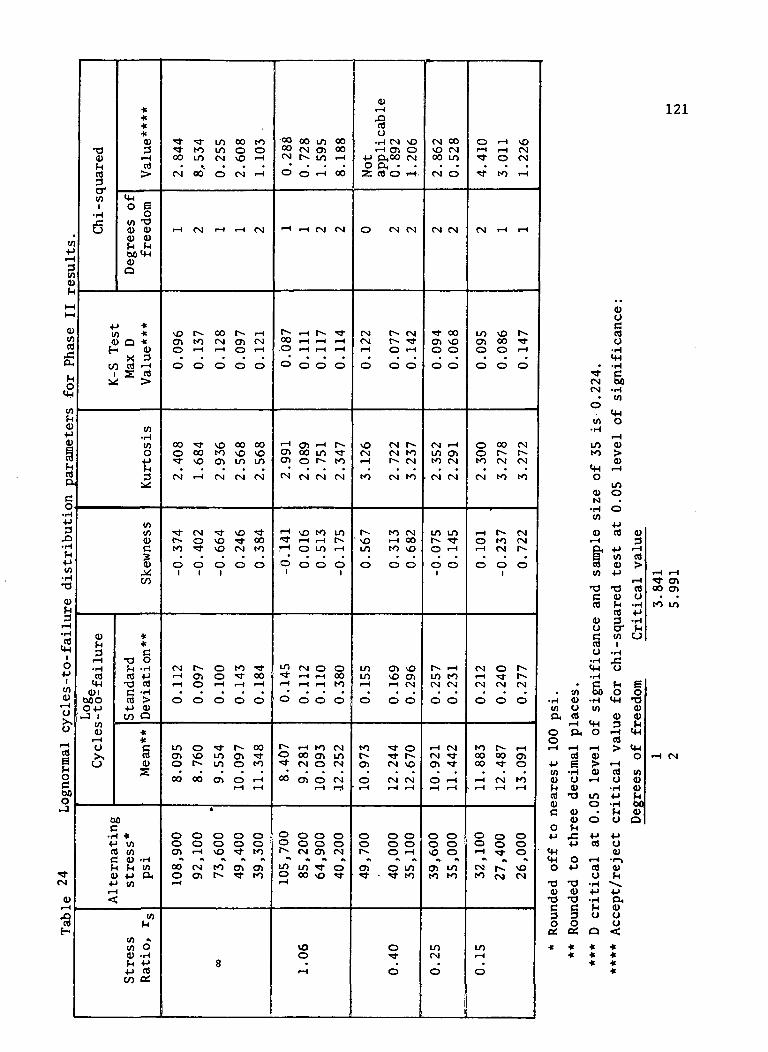
resu

lts.

t— I

0)COar-

(X

Ǥ

ram

ete

rs

n»P.

s•H4->3

rQ•Hf-l

4-><n•H13

<0H3rH•Hrt

<4H

O4->

1

0I— 10.

brHifnOC00oJ

•*!•CM

V

g

T3<u

(4

</)I

•H

6

4-U<

c/

u

f ai lure

<UIMOO4->

i-J 1(ft<DrHCJX

C_)

0c

•I"

•*-a

a4-^<

«***V31-1

De

gre

es

of

fre

ed

om

i *i *' Q *n' X 3) rt rH

< S : S

"to

sis

3^

(/)wd>C

0)^co

dard

atio

n**

C -Hcd >4-> 0)w o

*

*§0)s

pt *

> wI tn< !H </>) 4-> PH> W

10

^

« «(0 Oa> -HfH *->4-1 rtto cc

• f "* LO 00 to•*t to LO O Ooo LO rs vo i— '

(N 00 O tN i-H

rH (N r-l i-H <N

\O r~ oo r>- r-HO> tO CM CT> <NO ' r"1 O r™1

0 0 0 O 0

OO "* \O 00 OOo oo to \o vot V0 CT> LO LO

(N rH (N CM (N

•<t fM ^ \O •*r> o \o ^ ooto ^fr \o <N to0 0 0 0 0

1 1 1

<N f~- O tO ^~•H O> O •* 00

o o o o o

LO o •t r^ ooO» ^ LO OT '*o r~- LO o tooo oo o* o I-H

rH rH

a

o o o o o0 O 0 0 0 !O> rH \O ^ tO

oo CM to a> o>O O> t» ^ torH

8

OO oo LO OO°° (N Crt 00tN 1- LO rH

O O rH OO

"-1 rH CM CS|

£ rH 1- TTOO rH rH rHO rH rH rH

0 0 0 0

1-1 a> rH r~O» OO LO "*CT> O t*» to

fN CN CM (N

*~* vO tO LO"T rH rH 1J"1 O LO rH

0 o 0 O1 1

1/1 <N O O•* rH rH 00

O o O O

1 rH tO (NO OO Oi LO"* fNJ O CM

00 O> O <MrH rH

O o O O0 0 0 O1" Cvl Ol CM

tO LO ^ OO OO \O rt

vOorH

0)rH

•8o•H CM \OrH O> O

4-> {1.00 (M

2: cr) o i-i.

O CM (N

CM r~- CMCN r "*rH O rH

O 00

\O CM f~-CM (N tOrH I~~ (N

tO CM tO

r to CM• \O rH OO

LO to \O

0 00

LO O) V0LO vO O>rH rH (N

O O O

to •* oi •*!• r-O> CM \O

O CM CMrH rH rH

0 0 Oo o of^ O rH

a> o LO• t- • ^r to

o*a-o

CM OO\O CMOO LO

CM O

CM CM

Tj- OOOt \O0 0

0 0

CM rHLO attO CM

CM CM

LO LOr~ 'S-O rH

0 O1

1- rHLO toCM CM

o o

rH CMCM rj-O) **

O rH•H rH

0 0O 0vO 0

at LOto to

LOCM

0

O rH \OrH rH CM^ O (N

• f tO rH

CM rH rH

LO VO !-•at oo •*0 0 rH

0 0 0

O OO CMo t-» r-»tO CM CM

CM tO tO

rH 1"- CMo to CMrH CM t

0 0 Oi

CM O !*»rH TJ- t~^CM CM CM

O O O

tO r>- rHoo oo o*00 rl- O

rH CM tOrH rH rH

0 0 0O o O•H Tt O

OS t vOtO CM CM

LOrH

O

121

.• H

COcxo01-1

4JCO<UN0)a)C

O+J

^WMHo

CD13

§Oo:4

.toCPuat

i— iP<

atE•HU(U

00)rHX

o

4)"

§0a:

**

CMCM

O

• H

LOto

oa>N•Hto<DrH

c3to

T3Ca)

O0

U•H<4-l

&-H

•H1*0

(+4o

"«VrH

LOO.

o4-*CO

rHa)U•H

•HrHU

0

*4c

*

st

at

0.0

5

level

of

sig

nific

ance

04->

13(1)FH053to

•H

O

oC4H

0)3rH01

^

rHatO

•H

•H

^4U

4JO0)

•r-»

(Ufn

^J"a,(Uuu

****

V

rHa)>

^^ato•H

•H^jU

rH rH

oo at. .tO LO

E0

rQ

0)0)fH

<4H

O

COO

£4(30IDa

rH CM

122

Table 25 ' Endurance strength calculations for Phase II groovedspecimens at stress ratio of °°.

Alternatingstresspsi

34,921

32,868

30,815

28,762

i

>3

2

1

0

n.i

Successes

6

7

6

1

N = 20

in.

18

. 14

6

0

A = 38

A

54

28

6

0

B = 88

d = stress increment = 2,053 psi

X = lowest stress level = 28,762 psi

X = mean (estimate)

) f = X + d[A/N + 1/2] =.28,762 + 2,053 [ li + I]_ ° 20 2X = 3 3 , 6 8 9 psi a 33,700* psi

s = standard deviation'(estimate)

S = 1.620 d[(NB-A 2 ) /N 2 + 0 .029]= 1.620 (2,053) [ 20(88) - (38)2_ 0.029]

s= 2,724 psi = 2,700* psi (20)2

* Rounded off to nearest 100 psi.

Table 26 Endurance strength calculations for Phase II groovedspecimens at stress ratio of 1.06.

123

Alternatings. tresspsi

35,202

34,109

33,016

31,923

30,830

29,737

5

4

3

2

1

0

n.

Failures

1

3

8

3

4

1

N = 20

in.i

5

12

24

6

4

0.

A = 51

i2n.i

25 '

48

72

12

4

0

B = 161

d » stress increment = 1,093 psi average

X = lowest stress level = 29,737 psi

X = mean (estimate)

X = X + d[A/N - 1/2] = 29,737 + 1,093 [51 0.5 ]O --- —

Y= 31,978psi 2 3 2 , 0 0 0 * Psi 2 0

s - standard deviation'(estimate)

s = 1.620 d [ (NB-A 2 ) /N 2 + 0.029] = 1.620 (1,093)[ 20(161) - (51) 0.029]

5=2,796 psi £ 2,800 * pSi (20)

* Rounded off to nearest 100 psi.

Table 27 Endurance strength calculations for Phase IIgrooved specimens at stress ratio of 0.40.

124

Alternatingstresspsi

33,000

- 32,000

31,000

30,000

29,000

28,000

»

5

43

2

1

0

n.

Successes

1

23

6

7

3

N = 22

in.

5

8

9

12

7

0

A = 41

A25

32 -

27

24

7

0

B « 115

d = stress increment = 1,000 psi

X = lowest stress level = 28,000 psi

X = mean (estimate)

I = X + d[A/NO

X = 34,000 psi

s = standard deviation'(estimate)

S = 1.620 d[(NB-A 2 ) /N 2 + 0.029] = 1.620 (1,000) r22(U5)

s = 2 , 9 0 0 *

1/2] =. 28,000 + l,000[li 122 2

* Rounded off to nearest 100 psi.

125

Table 28 Endurance strength calculations for Phase IIgrooved specimens at stress ratio of 0.25.

Alternatingstresspsi

27,000

26,000

25,000

24,000

23,000

i

4

3

2

1

0

n.i

Failures

1

4

6

8

3

N = 22

in.i•

4

12

12

8

0

A = 36

.2in.i

16

36

24

8

0

B = 84

d = stress increment = 1,000 psi

X = lowest stress level = 23,000 psi__o r

X = mean (estimate)

"X = X + d[A/N - 1/2] =, 23,000 + 1,000[ it _ i ]

Y = 24,136 psi * 24,100* psi 22 2

£ = standard deviation'(estimate)

s = 1.620 d[(NB-A2)/N2 + 0.029] = 1,620 (1,000) [ 22(84) - (36)2

s =1,732 psi s 1,700* psi (22)'••• 0.029 ]

* Rounded off to nearest 100 psi.

Table 29 Endurance strength calculations for Phase II groovedspecimens at stress ratio of 0.15.

126

Alternatingstresspsi

25,000

24,000

23,000

22,000

i

3

2

1

0

n.

Failures

1

8

12

1

N = 22

in.

3

16

12

0

A = 31

.2lni

9

32

12

0

B *= 53

d = stress increment =1,000 psi

X = lowest stress level = 22,000 psi

X = mean (estimate)

X = X + d[A/N - 1/2] =. 22,000 + 1,000 [ ' £ ! _ £ ]X = 22,900^0,1 22 2

s = standard deviation' (estimate)

S = 1.620 d[(NB-A2)/M2 + 0.029] = 1.620 (1,000) f 22(55) - (51)2

S « 700* psa (22) 2Q2g

* Rounded off to nearest 100 psi.

<H atO C

OV) -H0) 4->^H 30.0X-HO h

SOO

(/)

CM VI

4~> t)« B

•HV) O4J <UrH ft3 Wt/1J) -afH a>X o4J Ooo HC 00

4J ^

LO

o

J-l3 -i

-U CDC <U<D 4->

10t-H1-H O

Tt0) toto "*

a co ooHH a)

o

o3 ••-( o

CO •-! O

oto

co•\

**0

0CD

'atC in

-H enB CDO rH2 •!->

in

CDC•H,0Boo

CO5

in10CDrH

i~H 4-*

C

's §O <DZ B

atB(HoC

a)CO

CO100rH

I/)

00rH Cat -HC *^•H CE <u

00C•H*->at

eCD1 jrHat

c/j"t>

*>COT) -H

inT3^jCO

^Ico^

*Cat -Ho in"S ft

D

*

CD•O -H

10

TJ+Jco

.co3

^•)C

fi

TO *rH0) toS P.

cd(/)

*•

<j)TJ -H

(/I

* QH

•O

co

atico

A

*CO -Hft\ if*V v)2 ft

toinin *CD OrH -H

CO COrH

O O O O0 0 0 Ot . OO OO rH

CM to r-« r-«

v

o o o oO O 0 Or* ^ ^ 10

• » » » • * *tO ^ rH O>*O " OO O)

o o oo o o

o \o CM o»CM r-> vo

0 0 0o o o

O CM O LO

O \O \Oto r** o^

o o o oo o o orv oo o> t -

• •» •» •«CM CM CM rH

O O O OO 0 O Of^ O 'S' rH

to CM o •^~tO tO tO CM

\o c^ 10O •«» CM

8 . . .rH 0 O

O0r--.,-j.

oo

*l

^^torH

O0

,-jT

o0

M

CMIO

o0

o0enCMCM

LO

.o

127

CM

•HCOftoo

4->

CO

rHCO(O

•oCD

z

COCO

D

II

co

a)COb

coD

§

CM

CM

l l rV(0

COco I in , a1 II rH IW

***

<4HO

4-> G(1) O

C 30) J3

C0)>0)

O 3<4H ^5

• H

0)(H

IA<D 13

• H(<-l

Cd4JCd

0) ci)C r<

T3 3O rHO -Hoo cd

<4H-O I<u ot-t 4->cd i3 </>cr oV) rH! O

•H XrC O

TJ rH

cd 0)w

to cd

to

tnutCU rH

4-> rH

13 OCD

Cd rH3 X>cr cd(A -H

• H Cd

a >

V)V

Tf\t/J

1

Co•H

X> tn•rH hrH 0)Ij Ij

(A 0)

•5 eelr*

rH Cd

3,0

CDS

DO

rH -H 60Cd 4-> C IAC ed -H tn, j C 3 O

1 s ££z +^ ,0 c/)

r^cd

**03

*4HO

(=(A OCD T31) OrH <UM rH<U "4-1O

*o a)3

^ <w?S TO

V)O

>- <->^0

V)(U

cr oXO

CV)

rH d>DH N£ 'iH3 tn

CO

§.HTO *rtcu tn2 PL,

tntn «0) OrH -H4-> H->CO Cd

(-1

Oi ^^ \O *«O C^OO rH tO CM • >

• r to •* oo CMO VO •* CM CM

CM rH

CM CM tO CM tO

\O - Tf CM O»00 (7) ^^ OO (7)O rH O O O

O O O 0 O

o o o o o0 0 0 O OO •* rH Ol rH

CM m Tt \o oorH LO

\o o to in oto \o in CM ooTf rH \O ^O OO

rH •— 1 O 00 rHrH tO

in oi oo inoo o to CM Is*tO t-H OO CM rH

LO m in m into to to to to

0 O O 0 0o o o o oO* rH \O ^" tO

CO CM tO Ok CHO O) t** *t torH

8

CM f-. O rH\O CM O toO m 10 CNo \o CM inrH

CM IO tO CM

CM to O oCM 00 O i-H<*H O rH f-t

o o .0 o

o o o oo o o o

. i-l to O

CM 00 CT> CftrH 00

"» C7> Cfl tOi*^ ^ oo GJvo co in ooCM CM LO tO

inrH

m CM rf r-.rH O OO Tt

tf CM rH rH

in in in into to to to

0 0 O O0 o O Of» CM Ot CM

in in - oO 00 vO ^tr-i

vO0

rH

O) O O)o en soi-H CM rH

to CN to

to CM to

•*!• o inCM r-« torH O rH

•0 0 O

0 O Oo o oCD O O0 0 Tl-^f ^f r^

rH rH

oo •* inrH rH Oin CM too o r^CM 00 t

rH

• - CM CMO 0 VO

CM CM rH

m in mto to to

o o oo o or- O rH

en o in^ ^ to

o.

o

O rHCM O

in vo

CM CM

O OrH 00rH O

0 0

0 O0 OvO C^

•<* o>CM in

rH Oin ooo inVO rHto •*

in toto inCM rH

in into to

o oo ovO O

o> into to

mCM

o

O> LO rHO vO CMCM tO rH

CM tO O»

CM CM IO

o> oo inI-- O rHO rH rH

o o o

0 0 Oo o oo m toto in o>Cft Ok O*

CM

vO 00 O•*3- CM vOin CM o>CM oo invO CO CM

rH CM

in oo i-HvO O> rr

rH CM rH

in t into to to

o o oO o OrH O

CM | vOM CM CM

LOrH

O

128

OI

10w0)

ioDO

cdU

•Hf-tO

CD

£

9)

0)

ino

•29)U

O•H

in

i-H -H

> ClO

VI<4HO

rH LOO rHOk OO

* •in i*»ii n6 6O O

•O T30> V0) 0)

•

TfCMCM

•0

0

0)3cd>

aCOi$4

*

•n0)0)

CO0)

TS

CM

•»4>

rHcd>

13g

cd3crwi•H<^

CJ

**

<n0)V

M0)•oIO

*Cl>3rHcd>

T3O

cd3crini•HXU

**

129

APPENDICES

APPENDIX A

POP PROGRAM TO CALCULATE VISICORDER DIVISIONS FOR 130DESIRED LEVELS OF BENDING AND TORQUE

C-8K MODV 11-219

01.09 T "MACHINE NO. 3", !, !, !01.10 T "STRESS RATIO = INFINITY", !01.20 A "STRESS LEVEL = ", SL, !01.30 A "BENDING CAL. RESIST. =", RB, !01.50 S Kl = 1.308101.60 S K2 = .017001.70 S K3 * .874801.80 S K4 = .054201.90 S K5 = .0645

02.06 S DS = .49102.07 S DO = 2.002.08 S DI = 1.312502.20 S NB = 5002.30 S NA = 402.40 S GB = 3.2302.50 S A = 3000000002.60 S BR = 19002.70 S NT = 4502.80 S GT = 2.0602.90 S TR + 120

03.10 S TO = 003.20 S SO = K2*K1*SL03.30 S SP = SO+K4*TO03.40 S VB = (NB*NA*GB*RB*SP)/(A*BR)03.80 T %7.03, "VIS. DIV. - BENDING", VB, !03.90 T %8.01, "BENDING CALIB.", RB," FOR 50 DIV.,", !

05.10 S EB = .03*VB05.20 S ET + .03*VT05.30 S SB + SL/VB05.50 T %5.02 "DIV. OF BENDING FOR 3% ERROR", EB, !05.70 T %8.01 "BENDING SENSITIVITY", SB," PSI/DIV.", !

131

APPENDIX B

PROGRAM STRESS (Updated)

The purpose of this program is to convert each Visicorder record

into normal stress, shear stress and stress ratio. The program

calculates the mean and standard deviation of these two stresses and

of the stress ratio of each group of cycles-to-failure data. It

calculates the cycles-to-failure from time-to-failure data. The

program will also accept cycles-to-failure data.

This program remains basically as described previously.

Added are the latest calibration coefficients and a routine to

convert shear stresses to normal mean stresses.

The program distinguishes between cycles-to-failure and time-to-

failure through the use of a code number. The code also tells the

program whether or not the group of data are endurance test data. This

discrimination is necessary because the program will not calculate the

endurance strength distribution parameters. The discrimination code

is fed in as data, and is as follows:

0 if the failure data is in time to failure.

1 if the data is endurance test data.

2 if the failure data is in cycles to failure.

132

The program will accept as many sets of data as desired and the

groups may be mixed; i.e., endurance test, group with cycles-to-failure

data, and group with time to failure data. A group is all the data

for one stress level. A group of data consists of the following: The

first card contains in this order, the number of specimens in the level,

the mode of the run and the code. The mode is dependent upon the date

the run was made and identifies the calibration constants for each

machine to be used in the computations.

The fields on the data card are as follows:

spaces 1 to 5 - number of specimens

spaces 6 to 10 - mode

spaces 11 to 15 - code.

The number of specimens, mode and code are fixed point numbers and have

no decimals but the numbers must be placed to the right in each field.

The next sequence of cards reads in the cycles-to-failure or time

to failure in hours, minutes and seconds. If the data is in time to

failure there are ten groups on a card, so the number of cards required

will depend upon how many specimens are in the stress level. The format

across the card is as follows:

spaces 1 and 2 - blank

spaces 3 and 4 - hours

spaces 5 and 6 - minutes

spaces 7 and 8 - seconds

spaces 9 and 10 - blank >

133

and the sequence continues in this manner. If the failure data is in

cycles-to-failure the format is 8 fields of 10 spaces each and the

decimals appear in the last space of each field; i.e. spaces 10, 20,

30, etc. If the group of data is for an endurance test there is no

failure data and these cards are left out. The program will automatically

' handle the data if the proper code number is put on the first card.

Following the cycles-to-failure cards are the cards containing the

information for each specimen in the stress level. The information

must be placed on each card as follows:

spaces 1 to 5 - test number

spaces 6 to 10 - specimen number

spaces 11 to 15 - machine number

spaces 16 to 20 - with a decimal in space 20 - pan weight

spaces 21 to 30 with a decimal in space 28 - bending calibration

resistance

spaces 31 to 40 with a decimal in space 38 - number of bending

calibration divisions

spaces 41 to 50 with a

decimal in space 48 - number of divisions of bending

spaces 51 to 60 with a

decimal in space 58 - torque calibration resistance

spaces 61 to 70 with a

decimal in space 68 - number of torque calibration divisions

134

spaces 71 to 80 with a

decimal in space 78 - number of divisions of torque

The test number, specimen number, and machine number are fixed

point numbers and must be placed to the right in each field. There

is one card for each test specimen and the cards must be placed in

the same order as the failure data is placed on the cards proceeding

these cards. For data at stress ratio of » there will be no torque

stress data. In this case these fields can be left blank. The

computer reads blanks on data cards as zeros.

This makes up one group of data at a given stress level and

ratio. As many groups may be run as desired by simply placing the

groups one behind the other.

A list of important variables and symbols in the program STRESS

using Fortran language follows:

135

List of Definitions for Program to Find

Stress Levels and Ratios (PROGRAM STRESS)

NCARDS

MODE

NCODE

XHOURS(I)

XMIN(I)

SECS(I)

TOTCY(I)

NOTES!

NOSPEC

MACHNO

PANWT

RCALB

ENCLAB

ENVISB

RCALT

ENCALT

ENVIST

ENA

= number of specimens tested at given level.

= number of mode depending on date of test.

= 0 if failure data is in times to failure.

= 1 if data is from an endurance level.

= 2 if data is in cycles-to-failure.

= times to failure in hours, minutes and seconds.

= cycles-to-failure.

= test number.

= specimen number.

= machine number.

= amount of weight on loading arm.

= calibration resistance used in bending channel.

= number of visicorder divisions used when calibrating

bending channel.

= number of divisions during actual test.

= calibration resistance used in torque channel.

= number of visicorder divisions used when calibrating

torque channel.

= number of divisions during actual test.

= number of active arms in strain gage bridge.

136RGAGEB

RGAGET

GB

GT

CBGR

CGRTH

CT

CTB

RPM

SOUTH

TAUTH

STRGR(I)

TAUGER(I)

SOUTHP

TAUTHP

resistance of bending strain gage.

resistance of torque strain gages.

bending gage factor.

torque gage factor.

calibration constant KD_n.BbK

calibration constant n „,„.bK- In

calibration constant 1C,.

calibration constant £„,,„.

revolutions per minute of machine.

output normal stress corrected for interaction.

output shear stress corrected for interaction.

normal stress in specimen groove.

shear stress in specimen groove.

output stress not corrected for interaction.

output stress not corrected for interaction.

The program STRESS listing in Fortran language follows:

137

PROGRAM STRESS ( INPUT, OUTPUT, TAPIE1 =INPUT)DIMENSION STRGRC50), TAUGR(50), R (50) , XHOURS (50 ) ,XMIN (50 ) ,1SECS(50) ,TOTCY<50)

C READ IN THE NUM9ER OF CARDS IN TH£ STRESS LEVEL AND THE M00£C OF OPERATION OF THE MACHINEC ----- NCOOE = 1 FOR ENDURANCE LEVEL, NCOOE = 0 IF FAILURES IN TIMES TO FAILURE.C ------- NCOOE - 2 IF FAILURES IN CYCLES TO FAILURE.35 REAO IOC, NCAROS, MOOF, NCOOE100 FORMAT (3i5>

IF (EOF,1> 201, 171171 PRINT 9191 FORMAT (1H1//)170 IF (NCOOE. EG. 1) GO TO 175C ----- FORMAT FOR OUTPUT HEADINGS INCLUDING TIMES TO FAILURE.

PRINT 310, MODE310 FQRMAT(62X,11HTEST HOOE =,I2/)

PRINT 6161 FORMAT (2X,3UHTEST SPEC. MACH. PAN CYCLES , 7X, <tHRC6L , 7 X

l,i*HNCAL,7X,t*HNVIS,6X,HHRCAL,6X,4HNCAL,6X,'»HNVIS,5X,7Hr»ENOlNG,^X, 126HSHEAR STRESS/ 3X , 35HNO . NO. NO. WT . TO FAILURE, 3X,37H3ENOING, t»X,7H8ENDING,t*X,7HB£NOING,<fXt6HTORlUE,<+X,5HTORGUE , VX,i+6HTOROUE,5X,6HSTR^SS,i»X,6HSTRESS,4X,5HRATIO//)IF (NCODB.EQ.2) GO TO 320

c ------ ROUTINE TO READ IN TIMES TO FAILURE.R E A D < + 0 1 , ( X H O U R S ( I ) , X M I N ( I ) , SEC3 ( I) , 1 = 1, N C A R O S )

i»31 F O R M A T (13 ( 2 X , 3 F 2 . 0 »GO TO 3CO

C ----- READ IN CYCLES TO FAILURE.320 READ <»02, (TQTCY(I), 1=1, NCAROS)402 FORMAT ( 3F1Q.O)

GO TO 300C ----- FORMAT FOR OUTPUT HEADINGS WITHOUT TIMES TO FAILURE.175 PRINT 90, MOOE90 FORMAT ( 50 X , 1<*HENQU9ANCE TEST , 10X , 11HTEST MOOE =,I2/)172 PRINT 60

60 FORMAT ( 3X , <*HT EST , 3X ,8HSP£CIMEN , 3X ,7HMACHI NE ,5X,3HPAN,7X,<*HROAL,7X

25HSHEAR,'+X ,6HSTRESS/«+X, 3HNO . , 6X, 3HNO. ,7X,3HNO. , 5 X , f>HW£ IGHT , 4 X ,37H8£NOING,4X,7HgENOING, i tX,7He£NOING, i+X, r ,HTOP.QUE,*+X,6HTORQUfc , uX,W6HTORQUf ,5X ,6HSTRESS,UX,6HSrR£SS,<+X,5HRATIO/ )

----- ROUTINE TO CALCULATE POLAR MOMENTS OF INERTIA.----- SPOIA = SPECIMEN OIA. TOO = TOOLHOLOER 0. 0. TIO = TOOLHOLGER I, 0.

300 SPOIA=.<*91CTOD=2. 0TIO=1.3125SPJC=(3.1<*159*SPDIA**3)/16.0THJC = (3. mi59*(TOO**<+-TIO**<»)) / (16.*TOD)CONST-THJC/SPJC00 120 I = 1, N C A R O SREAD IN THE TEST NO,, SPECIMEN NO., MACHINE NO., P A N W E T G H T , £NO THE

138

10

CC

CALIBRATION RESISTANCE', VISICOROER CALIBRATION DISTANCE ANDOUTPUT DIVISIONS FOR BENDING AND TORQUE

ftO READ 1Q,NOTEST,NOSP£C,MACHNO, PANWT, RCAL8, ENCALB ,£NVISR t RCALT ,1ENCALT.ENVISTFORMAT C3I5,F5,Q,6F10.2)CARDS = NCARDS0-FINE TH? ELASTIC MODULUS, NO. OF ACTIVE ARMS OF THE BRIDGES,RESISTANCES OF THE BENDING AND TORQUE GAUGES, AND THE RENDINGTORQUE GAUGE FACTORS£=30000000.

THE

15

RGAGtB=19Q.RGAGET=120.G9=?.23GT=2.06SELECTION OF MACHINE ANO MODEIF CMACHNO.EQ. LAND. MODE. EQ.l) GOIFCMACHNO.EQ.2.ANO.MODE.EQ.1) GOIFCMACHNO.EO.3.ANO.MODE.EO.l) GOIF (MACHNO.EQ.1.AND.MOOE.£Q.2) GOIFCMACHNO.EQ.2.ANO.MODE.EQ.2) GOIFCMACHMO.EQ.3.AND.MODE.EQ.2) GOIFCMACHNO.EQ.l.AND.MODE.EQ.3) GOIFC1ACHNO.EQ.2.ANO.MODS.EQ.3) GOIFCMACHNO.EQ.3.ANO.MOOE.EQ.3) GOIFCMACHNO.EQ.l.ANO.MODE.EQ.<4) GOIFCMACHNO.EQ.2.ANO.MODE.EQ.k) GOIPCMACHNO.EQ.3.ANO.MODE.EQ.it) GOIFCMACHNO .EQ. 1 .AND. MODE .£0.IFCMAoHNO .EQ. 2 .ANO. MOD- .dQ.IFCMACHNO .EQ. 3 .AND. MODE .EC.CALIBRATION PARAMETERS FQ* GIVENC^GR = 1.0123CGRTH - .0203CT = .3752CT3 = -,0'+5QC3T = .029

TO 11TO 2kTO 31TO 11TO 2kTO 31TO 11TO 2kTO 33TO 11TO 2kTO 7k5) GO TO 155) GO TO 255) GO TO 53MODE AND MACHINE

GO TO 50

•2k

CT=0.87g3CT8=-0.0<*62

PPM - 1779GO TO 50C3GR = 1.0123CGRTH = .0183

139

CT = .8201CTP = 0. 034<+C3T = . 0 4 2 2RPM=1784.GO TO 5G

25 C*GR=1.3091CGRTH=0.0145C T = 0 . 8 9 ? QC T R = 3 . 0 < * 6 3

= 1775GO TO 5C

31 C9GR = 1.1946CGRTH = .0211CT = .933CT8 = .0C-1T = - ,G1«»9

: R°M=178C.GO TO 50

33 CRGR = 1.0946: CGRTH = .0211

CT = .7721CTB = .CCBT = -.0127RPM=173G.GO TO 5C

34 CBGR = 1.0123CGPTH = .31Q7CT = .7721CTB = .0

C3T = -.0127R.PM-1780.

53 CBGR=1.3C31C G R T H = 0 . 0170C T = 0 . 8 7 t 8CTB = 0 . 0 5 4 ?CBT = G. 0645RPM = 1773GO TO 50

50 I F C E N V I S T . ^ O . O . O ) GO TO 160GO TO 51

C C A L C U L A T I O N OF SENDING STRESS LEVEL FOR INFINITY RATIO160 SOUTH=(EN\/ISB*E*=>GAGF.f»)/( i£NCALR*ENA*G8*RCAL8)

S T R G R ( I ) = SOUTH / (CGRTH * C 9 G R )TAUGR( I ) = O.CIF (NCODE.EO. l ) GO TO 301IF (MCODE.E0.2) GO TO 330

C ----- CALCULATE CYCLES TO PAILURE FROM TIMES TO FAILURd.CYHR = XHOUf iS( I )*60.*PPMCYMIN = XMIN(I)*RPH

140

CYSEC = < S E C S ( I ) * R P M ) / 6 0 , U; TCY = CYHR+CYMIN+CYSECi GO TO 335;330 TCY = T O T C Y ( I )'.335 PRINT 7 2 , N C T E S T , N O S P E C , M A C H N O , F A N W T , T C Y , R C A L C V E N C A L B , E N V I S 8 , S C A L T ,; i E N C A L T , E N V I S T , S T R G R ( I ) , T A U G R U >'72 FORMAT(3I6,F8.1,2F11.0,F13.2,F11.2tFl l .O|F10.2,

lF10.2, r l l . 0 , F l G . O , i + X , 6 H I N F I N . / )j GO TO 120301 PRINT 71,rtOT£ST,NOSPEC,MACHNO, PANWT ,RCALB ,ENCAL 8, C.NVIS3 , RC ALT ,

1ENCALT,ENVIST,STRGR(I),TAUGR(I)71 FORMAT(«»X,I3f 6X,I3,8X,Il,6X,FiJ.l,Fl2.0,F10.2fF11.2,Fli.C>Fia.2»

1F10.2»F11. 0,FlO.Oi3X,6HINFIN./)GO TO 120

C CALCULATION OF BENDING STRESS, SHEAR STRESS AND STRESS RATIO FORC ALL FINITE RATIOS

51 SOUTHP=(ENVISB*E*RGAGF8)/(ENCAL8»ENA*GB*KCAL^)TAUTHP=(ENVIST*E*RGAGET)/<ENCALT*£NA*GT*RCALT)SOUTH=SOUTHP-CTB*TAUTHPTAUTH=TAUTHP-CST*SOUTHSTRGR(I) = SOUTH / (CGPTH * C^GR)TAUGR(I) = CT*TAUTH*CONSTR(I) = STRGR(I) / (TAUGR(I) * 1.73?)IF (NCODE.EO.l) GO TO 302IF (NCODE.EQ.2) GO TO 3UC

C CALCULATE CYCLES TO FAILURE FROM TIMES TO FAILURE.CYHR = XHOURS(I)*60.*RPMCYMIN - XHIN(I)*RPMCYSEC = (SECSCI)*PPM)/60.0TCY = CYHR+CYNIN+CYSECGO TO 3^5TCY = TOTCY(I)PRINT 73.NOTEST, NOSPEC,MACHNQ,PANW7,TCY,RCAL3,ENCAL3,£NVISe,=CALT,

1ENCALT,ENVIST,STRGR(I),TAUGR(I),S(I)77, FORMAT(3I6,F1.1,2Fli.O,FlJ.2,FH.2,Fi1.c,F10.2,

1F10.2,FH. o,Fio.O,F9.3/)GO TO 120

302 PRI^T 70,MOTEST,NOSPEC,HACHNO, PANWT,RCALO,ENCALn,ENVIS3,RCALT,1ENCALT,ENVIST,STOGR(I),TAUGR(I),R(I)

70 FOR*ATUX,I3,6X,T3,3X,Il,6X,F5.1,FlP.O,FiC.2,F11.2,Fll.C,FiQ.2,lF10.2,F11.0,F10.0,Fg.3/>

120 CONTINUEIF (NCODE. EQ. I.ANO.ENVIST.EQ.O.O GO TO 35Ip !N.CpDE.EQ.l)_ GO TO 200 _ _

c " C A L C U L A T I O N OF MEAN AND sTANDAPb~o£viAfi 'oM OF RENDING S T R E S S , SHEAPC STRESS, AMD STRESS RATIO

CALL MEAN (STRGR, CARDS,NCAPQS, XMEAN, OEV)PRINT 3

3 FORMAT (1H )PRINT 130, XMEAN, OEV

141

130 F3P.1AT <19X,31HMEAN BENOING STRESS IN GROOVE =, F 10. 1 ,5« PSI.//11X,139HSTD. DEV. OF BENDING STRESS IN GROOVE. =,FlG.2,5H PSI./)

•132 IF(ENVIST.EQ.O.O) GO TO 35IP (NCODE.EQ.l) GO TO 200CALL MEAN (TAUGR, CARDS, NCARQS, XMEAN, DEV)PRINT 3PRINT H»0i XMEAN, 0£V

ii»o FORMAT (2ox,30HMEAN TORQUE STRESS IN GROOVE =,Fio.i,5H PSI./ i2x,133HSTD. DEV. OF TORQUE STRESS IN GROOVE =fPlQ.2,5H PSI. )SMEAN = XMEAN*!. 732SDEV = OEVM.732PRINT 3PRINT 1&2, SMEAN, SDEV

1<*2 FORMAT(19X, *MEAN NORMAL STRESSSIN GROOVE*, F10.1, * PSI.*//11X,1*STQ. OEV. OF NORMAL MEAN STRESS IN GR =*, FIG. 2, * PSI.*/)

200 s CALL MEAN ( R, C ARDS , NCAROS , XMEAN, DEV)PRINT 3PRINT 150, XMEAN, OEV

150 FORMAT CUX,19HMFAN STRESS RATIO =,F10.5/ 23X,27H.STO. OEV. OF1SS RATIO =,F10.5>

37 GO TO 35201 STOP

ENDSUBROUTINE MEAN (X, DATA, NOATA, XMEAN, DLV)

C ----- SUBROUTINE TO CALCULATE THE MEAN AND STANDARD DEVIATION OF DATA.DIMENSION X(NHATA)SIGMA= C.ODO * 1=1, MDATA

XMEAN = SIGMA/DATATOP2 = 0.0DO 9 I=1,NDATATOP2 = TOP2 * (X(I) - XMEAN)**2OEV =SQPT(TOP2/(DATfl - 1.0))RETURNEND

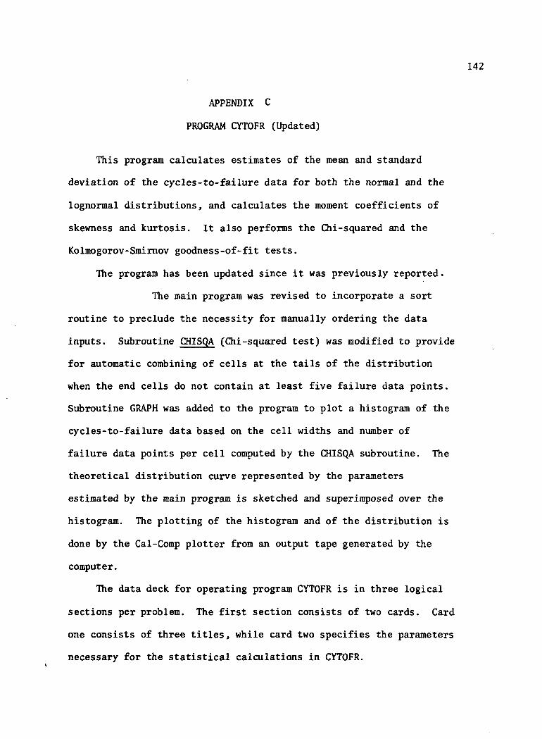
142

APPENDIX C

PROGRAM CYTOFR (Updated)

This program calculates estimates of the mean and standard

deviation of the cycles-to-failure data for both the normal and the

lognormal distributions, and calculates the moment coefficients of

skewness and kurtosis. It also performs the Chi-squared and the

Kolmogorov-Smirnov goodness-of-fit tests.

The program has been updated since it was previously reported.

The main program was revised to incorporate a sort

routine to preclude the necessity for manually ordering the data

inputs. Subroutine CHISQA (Chi-squared test) was modified to provide

for automatic combining of cells at the tails of the distribution

when the end cells do not contain at least five failure data points.

Subroutine GRAPH was added to the program to plot a histogram of the

cycles-to-failure data based on the cell widths and number of

failure data points per cell computed by the CHISQA subroutine. The

theoretical distribution curve represented by the parameters

estimated by the main program is sketched and superimposed over the

histogram. The plotting of the histogram and of the distribution is

done by the Cal-Comp plotter from an output tape generated by the

computer.

The data deck for operating program CYTOFR is in three logical

sections per problem. The first section consists of two cards. Card

one consists of three titles, while card two specifies the parameters

necessary for the statistical calculations in CYTOFR.

143

The second, logical section is a variable number of cards, each

specifying up to eight data points for analysis.

Section three provides parameters for plotting the normal and

lognormal distributions. The first card is a parameter list for the

normal distribution plot, followed by exactly six cards of footnotes.

Next is a parameter list card for the lognormal distribution.

Multiple problems may be executed by stacking complete data sets

behind each other. A list of important variables and symbols in

program CYTOFR using Fortran language follows:

144

List of Definitions for Program to fit Normal

and Log-Normal Distributions to Cycles-

to-Failure Data (PROGRAM CYTOFR)

Main Program:

NDATA = DATA = number of observations.

STRLV = stress level in psi.

AKURCY = accuracy to which cycles-to-failure data are known.

RATIO = stress ratio

X(I) = cycles-to-failure data

CUMFRQ(I) = cumulative frequency of each X(I); ie, number of

X's less than or equal to X(I).

PCAREA(I) = CUMFRQ(I)/NDATA

Subroutine to calculate the mean and standard deviation of the

cycles-to-failure data (SUBROUTINE MEAN)

SIGMA = sum of the X(I)'s

XMEAN = average of the X( I ) 1 s

n 2TOP2 = Z (X(I)-XMEAN)

i=i

DEV = standard deviation of the X(I)'s

Function subroutine to find the area under the normal curve

(FUNCTION PROB(X)).

X = abscissa value for which corresponding area

is desired.

PROB = desired area.

145

Subroutine for Chi-square goodness-of-fit test (SUB-ROUTINE CHISQA).

K = number cells.

XMAX = largest value of cycles-to-failure.

XMIN = smallest value of cycles-to-failure.

CSV = cell starting value.

CEV = cell end value.

CLB = cell lower bound.

CUB = cell upper bound.

FREQ(J) = number of observations in J**1 cell.

REQAREA(J)= expected value of Jth cell.

CHISQR = total Chi-square value.

U(I) = Chi-square value of Ith cell.

Subroutine for Kolmogorov-Smirnov test (SUBROUTINE DTEST).

Z(I) = abscissa value on standard normal curve for a

given X(I).

ARUNCN = area under standard normal curve from - to Z(I).

DSTAT(I) = absolute difference between the data cumulative

frequency and the hypothesized cumulative frequency.

XMEAN = average of the X(I)'s.

DEV = standard deviation of the X(I)'s

PROB(T) = area under the standard normal curve from -T to

+T.

146

Subroutine to calculate the moment coefficients of skewness and

kurtosis (SUBROUTINE ALPHA).

ALPHAS = moment coefficient of skewness.

ALPHA4 = moment coefficient of skewness.

VAR = Z (X(I)-X)

TOPS

SKEW

STDEV

TOP4

TKURT

= £ (X(I)-X)- 3

= third moment of the data.

= biased estimator for standard deviation.

= Z (X(I)-X)4

= fourth moment of the data.

147

DATA DECK STRUCTURE

Card

1

Columns

1-20

21-40

Description

Twenty character descriptive titleto appear at the top of each printedoutput page.

Twenty character descriptive title ofthe input data will appear on printedoutput,as well as the X-axis label forboth slots.

41-50 Unit of data measurement (cycles, inches,etc.).

1-10 Number of data points on followingcard(s). Must have a decimal point.

11-20

21-30

31-40

3 to n** 1-10, 11-20, ...,71-80

n + 1 1-10

Stress level. Must have a decimal point.

Stress ratio. Must have a decimal point.

Accuracy. Must have a decimal point.

Data points, punched eight per carduntil all points are exhausted. Musthave decimal points.

The letters "NORMAL" followed by fourblank spaces.

11-20

21-30

Length of the X-axis in inches. Ifzero or blank, 6.0 is assumed. Decimalpoint is necessary.

Length of the X-axis in inches. If zeroor blank, 5.0 is assumed; if greaterthan 5.0, 5.0 is assumed. Decimal pointis necessary.

**The notation 3rd to n is intended to mean from the third card to the nthcard. In the case of 34 data points, the second section of data wouldstretch from the 3rd to 7th card .

DATA DECK STRUCTURE (Continued)148

Card Columns

31-40

41-50

51-60

61-70

Description

Minimum X-axis value. The plottingprogram may find it necessary to alterthis value slightly. If absent orzero, a resonable maximum will beassumed. The decimal point is necessary,

Minimum Y-axis value,blank or 0.

This should be

Maximum X-axis value. Follow samerules as minimum X-axis value.

Maximum Y-axis value. If absent or zero,the plotting program will search for thesmallest even number greater than Corequal to) the height of the tallesthistogram block, an automatic adjustmentwill be made. The decimal point isnecessary.

n + 2 ton + 7

71-80

1-50

Height of lettering on graph, if 0 <height < .15. Otherwise this parameterwill be set to equal .15.

Footnotes punched as they will appearon the normal graph.

n + 8 1-10 The letters "LOG-NORMAL."the same as card n + 1.

Otherwise

The program for CYTOFR listing in Fortran language follows:

149

PROGRAM CYTOFR ( INPUT , OUTPUT, TAPE l^INPUT , TAPE2 )C ----- PROGRAM TO FIT NORMAL AND LOG-NORMAL CURVE TO D A T A AND CHECKC ----- GOODNESS OF FIT.

COMMON CUMFRQC100) , NO AT A , X ( 100) , DEV, XM£ AN, CLB ( 9) ,C'JR<9) , F R £ Q < 9 > »<»1 CHI SQR, TITLE (2) ,SUBTITL<2) ,CSV { 9 ) ,CEV (9) , PCARE A ( 100 ) , O S T A T ( l u Q ) .2 A SEA (9) , R F Q A R E A < 9 ) , E X F R £ 0 < 9 > ,U ( 9) , Z ( 100 ) ,NX ( 10 0 ) , D A T A , AKIHCY ,3 X H A X , X M I N , P S I , C D , D » R A T I O , X L E N G T H , Y L E N G T H , Y M A X , YMIN, X1A , XMI ,<* H L E T T E R , C O M ( 3 ) t W, ALPHAS , ALPHAS FOOT ( 30) ,IT,SKS,UNIT

INTEGER TITLE, SUBTITL, FOOTEXTERNAL °ROB

CC INITIALIZE PLOTTERC

CALL INITIAL (0 ,2 ,0 .3 ,0 )710 PRINT 1G ----- N D A T A = O A T A = N U M B E R OF OBSERVATIONSC ----- STRLV = S T R E S S LEVEL IN PSI.C X=NUMBER OF CYCLES TO FAILURE

REAO 5 o C , TITLE, SU9TTTL, UNIT5 0 0 F O R M A T ( e A l O )

IF(EOF(D) 56,55 REAO 501, O A T A , S T R L E V , PATIO, A K U F C Y

501 F O R M A T ( 8 F 1 C . O )N D A T A = D A T 4REAO 501, (X<I ) , I=1,NOATA)

CC SORT X( I ) TERMS IN ASCENDING O R C E R .C

K=NOATA-1IF(K.LE.O) GO TO 30DO 20 1 = 1, KN=N1ATA-IIST03=000 10 J=1,NIF(X(J) .LE.X(J*1)> GO TO 10S A V E = X ( J )X ( J ) = X ( J + 1 )

ISTOP=ISTOP+11C CONTINUE

IFdSTOP.EQ.OI GO TO 3D2C CONTINUE

CC SET CUMFROm A R R A YC

30 00 <»0 I=1,NCATA

CC RESET SOME CUMFRO(I) ENTRYS IF X( I )=X(I*1) OCCURS

150

n00 50 I=2,NDATA

50 CONTINOtG PCA*£A - r(N) Of OBSERVATIONS

DO 759 1=1, NDATA759 PCARIA(I) = CUMFRQ(I)/DATA

PRINT *08,TITLE,SUBTITL<406 FORnAT(*l*,55X,2A10,/,<*2X,*NORMAL DISTRIBUTION FITTED TO *,2A10»

I///)IF (RATIO.£0.0.0) GO TO <*!<*PRINT i*C2, STRLEV, RATIOFORMAT(29X,*STRESS LEVEL =*,F7.1,* PSI.*f16XtlitHSTRESS RATIO =,F6GO TO <r!5PRINT t!6, STRLEV

FORMAT(29X,*STRcSS LEVEL =*,F7.1,* PSI.*,16X1,23HSTRESS RATIO = INFINITY//)PRINT ^0«f,SUBTITLFGRMAT(5f.X,2A10,/)PRINT <*03, (X(I) ,I=1,NOATA)

PRINT .5FORMAT (1HO)C A L L "IcANCALL C H I S Q ACALL O T E S TCALL ALPHAREAD 502, I T , X L E N G T H , Y L E N G T H , X M l , Y M I N t X M A , V MAX ,HL t TTER

50? FORMAT (A l , 9V, 7^10. 0)

503 FORMAT (5 A 1C)Ir (IT.NE.1HN) GO TO 57CALL GRAPH

5 3 A K U R C Y = . C Q C O iDO 5* I=1 ,NOATAN X ( I ) = ( A L O G ( X ( I ) / 2 0 . ) + A L O G ( 2 0 . ) ) * 1 Q O O O G . + .5X(*I) = NXd)

PRINT 1, TITLE1 FORM4T(*1*,55X,2A10)

PRINT 4C1,SU-3TITLnOl FORMAT (3flX,*LOr,-K/ORMAL DISTRIBUTION FITTED TO *,2AlO,///l

IF (RATIO. EO. 0.0) GC TO kl?PRINT ifC2, STRLSV, RATIOGO TO i»13

<f!7 PRINT i»16, STRL£Vi*18 PRINT 2,SUf3TITL

2 PORMAT (U9X,*LOGS 0^ THE *PRINT Hl3, (X(I» ,I=1,NOATA)

151

F O R M A T ( 6 ( 9 X , F 1 2 . < » )PRINT 3CALL MEAN

C A L L O T E S TCALL ALPHAREAD 5 0 2 , I T , X L E N G T H , Y L E N G T H , X M I , Y M I N , X M A , Y M A XIF(IT.NE.1HL> GO TO 57C A L L GRAPHGO TO 7io

56 C A L L PLOT (0. ,0.,999JCALL EXIT

57 CALL PLOT <0 . ,0 . ,999)STOP tillENDSUBROUTINE MEAN

C ----- SUBROUTINE TO CALCULATE THE MEAN AND STANDARD DEVIATION OF DATA.COMMON CU*IFR.a<lOO> , NO AT A, X < 100 ) ,DEV, XME A N, CL8 ( 9) ,CU9(9) ,FRFQ(P) ,K,

1 CHI 3QR, TITLE (2) ,SUBTITL (2) , CSV (9 ) ,CEV (9 ) , PCARi A ( 100) , D S T A T ( 1 Q O ) ,2 A R E A (9) , R E Q A f ? E A ( 9 ) , EXFREQ (9) ,U (9) , Z ( 10 0 ) , NX (1 J 0 ) » DAT A , AKIHCY »3 XHAX,XMIN ,PS I ,CO,0 ,R ,XL£NGTH,YLENGTH

SIGMA= 0.0DO 4 1=1, NOATA

3 SIGMA=SIGMA+ X(I)XMEAN = SIGMA/OATATOP2 = 0.0DO 9 1 = 1, NOATA

9 TQP2 = TOP2 * (X(I) - XMEAN)**2DEV =SQPT(TOP2/<OATA - 1.0»PRINT !«., XMEAN

PRINT 15, DEV14 FORMAT (iox, 'SAMPLE MEAN -*,Fiit.;»)15 FOR*AT(1QX,*STO. OEVI ATION = * , F12. •+)

RETURNENDFUNCTION PROB(X)

0 ----- THIS SUBROUTINE GIVES AREA UNDER NORMAL CtJRV£ FPQM -Z TO +ZC WITH AN ACCURACY OF O.OOC05C ----- Z VALUF GIVEN BY CALLING PROGRAM MUST BE A POSITIVE NUMBER.

IF (X-l. 2) 11,11,1211 XSQ=X»X

PRO^= 0. 7978 8<»55*X*(0 . 9999977 4 - X S Q * ( 0.1 665 9<*33-X SO* (0. 02^6 3^ T 1 0 - X S1Q*C. 002397<*8 fa7»»

RETURN12 I F ( X - 2 . 9 ) 13,1<»«1<»13 X S Q = X * X

PROB=1.0PTERM=1. 0FACTOR=1.0

152

970 P T E R M = - P T £ R M * X S Q / ( 2 . 0 * F A C T O R )TEPM-PTERM/ODDINTPR09=PROB+TERMIP( ABS (TERM) - C.00007 ) 80,90,90

90 FACTOR =FACTOR-H.OODOINT = ODDINT*-2.0GO TO 970

80 PR03=0 .79788<+55*X*PROBRETURN

1<+ RECXSQ* 1.0 / ( X * X )PR03= 1.0 - 0 . 7 9 7 8 8 U 5 3 » £ X P ( - X * X / 2 . 0 ) / X * ( 1 . 0 - R E C X S Q * ( 1 . - P £ C X S G * ( 3 .

1 - RcCXSO*( l5 . - RECXSQM05. ) ) ) )RETURNENDSUBROUTINE CHISQA

C SUBROUTINE TO FIT A HISTOGRAM TO THE DATA AND PeKpORM THE CHI-SQUAC TEST FO& THE NORMAL OR LOG-NORMAL DISTRIBUTIONS.

COMMON CUMFCQ(IOO),NDATA,X{100),D£V,XMEAN,CL3(9) ,CUB(9),FRcQ (9),K,1 CHISQR,TITLE<2) ,SU8TITL(2),C3V(9) ,CEV(9) ,PCARtA(100),03TAT (100),2 AREA(9),REQAREA(9),EXFRiO(9> ,U(9),2(100) ,NX(100 I,OATA,AKURCY,3 XMAX,XMlN,PSI,CO,0,R,XLENGTH,YLENGTH,YMAX,YMIN,XMA,XMI,HtCOM(3),WDIMENSION XFR£Q(9)f^LJTon^'^ rtonx.jvj"'~»u

n TO DETERMINE THE NUMBER OF CLASS INTERVALS,KK= 1 +3.3 "ALOGIO(OATA)

C ----- IN ORDER' TO OETEPMINE THE RANGE, FIND X ( M A X ) AND X(MIN)

X M I N = X ( l )DO 17 I=1,NDATAIF( X ( I ) . G T . X M A X ) X M A X = X ( I )

17 IF (X( I ) .LT . XMIN) XMIN=X( I )RANGE= X M A X - XMIN

C ------ TO DETERMINE THE C L A S S INTERVAL WIDTH, WC ----- ROUTINE TO ROUND OFF CLASS WIDTH TO SAME NUMBED OF P L A C E S A5 TH'l A

DIVIDE = l . C / A K U R C Y2C K W = ( ( ( R A N G E * A K U < ? C Y ) /REALK) •»• . 5* A K U R C Y ) »OIV IDE

RX1 -. KIJW - RK1/DIVIDEDO 22 1=1, KA = IB = 0 .5 *A<URCYC S V ( I > = XMINMA-1. 0 ) * WC 'V( I )= C S V ( I ) * W - A K U R C Y

CL8( I )= C S V < I ) - R22 CUB( I ) = C E V ( I ) + B

CEV«) = XMAXC U 9 ( K > = CEV(K) *B00 23 J=1,K

153

XFR£Q(j')Vti"."F23 F R E Q ( J ) = O . G

00 2* I=1,NDATA00 24 J=1,KIP(XU) . G £ . C L B ( J > . A N D . X < I > .LT.CUB(J) ) FR'dQ ( J) = FREQ ( J) «• 1. 0

24 CONTINUE03 25 J=1,K

25 XFR£Q( J)=FREO(J)Y = 0 .PRINT 6 2 , X M A XPRINT 63,XMINPRINT 65, W

C ----- CHI-SQUARE T£ST26 PRINT 41

PRINT 406DO 30 1=1, KZ ( I ) = ( CU9(D- X M £ A N ) / OEVT= A 3 3 ( Z ( I > >

3 0 A R E A ( I ) = P K O R ( T ) / 2 . 0R E Q A R E A ( l ) = 0.5 - AREA( l )

MANU=K-100 32 I=2,MANUM=I-1IF ( (Z( I ) . G E . O . O . A N O . Z ( M ) , G E . O . O ) . O R . ( Z < I ) . L c . O . C l . A N O . Z ( M ) . L £ . a

1 ) ) GO TO 31

GO TO 3231 R £ O A R £ A ( I ) - A 8 S ( A R E A ( I) -ARE A32 CONTINUE

R £ Q A R E A ( K ) = 0 . 5 - A R E A (K-D00 30 M = 1 , K

30 E X F R E Q ( M ) = O A T A * R £ Q A R £ A ( V 1 )1 = 1IFC^REOd) .GE.5.) GO TO 2430

00 2^25 L=l,vJEXFR£Q(L)=0.

2425 FREQ(L)=0.1 = 1*1GO TO 2U2Q

2*30 I=K2ut*0 IF(FREO(I) .GE.5.) GO TO 2*50

£XFRtQ<I- l )=EXFREQ(I - l )+EXFR£;m)

00EXFR£Q(L) = 0.

2445 FREQ<L)=0.1=1-1

154

GO TO2(*5C CONTINUE

00 85 M=1,KU ( M ) = 0 . CI r ( IXFR£;Q(M) .EQ .Q . ) GO TO 35LMM) =( ( E X P R E Q ( M ) - F R E Q ( M ) )**?;

35 CONTINUE00 90 M=1,K

90 CHISQR=CHISQR+U(K)

C ----- TO PRINT THE TABLE FO* CHI-SQUARE TEST00 33 1=1, K

33 PRINT 3<+,I ,CLR(I) ,CUB(I) , £ < F 3 E Q < II t FRCCH I) ,U< I)P^IMT 3?, CHIS0300 150 1=1, K

150 F R £ Q ( I ) = X F F E Q ( I )6? FORMAT ( 1 Q X , * M A X I M U M V ALU£=* , F13. k)63 FORMAT (1GX*HINI!1UM V A L U E - * , F13.<+>65 FOR1AT(10X , *CLASS WIDTH=» , F 15. )

*1 F O R M A T C lH< j iit 06 FORMAT ( 3 X , 5 H CELL , 1Q X, 1GHLOWER C£LL,11X , IDH'JPPIR C^LL , 1 2X , 1 H £ X P P G

213X, 3HBOUNOARY,13X,9HFR£QU£NCV,12X,9HFRtQUENCY, 12X, 13HVALU,! CF Ct3LL/>

35 F Q H " 1 A T ( * 0 * , 7 7 X , * T O T A L CHI-SQUAF.EO VALUt -*,Fl3.u)RETURNENDSUBROUTINE OTEST

C ----- SUBROUTINE TO C A L C U L A T E THE KOLMCGO*OV-SMIRNOV O-VALUES.COM10M C U M F R Q ( 1 0 0 » , NO AT A , X ( iCi 0 ) , 0£V, XMEAN, OLO (9) , CUB (9 ) , FR£ H9 ) , K ,

1 C H I S Q R , T T T L E ( 2 ) , S U T T I T L ( 2 ) , CSV ( 9 ) .CEV ( 9) , =CflKE A ( 100 ) , DSTA T ( 1 DC ) ,2 A R E A (9) , R E O A R E A (9) , E X F R £ Q ( 9 ) ,U ( 9) , 7 ( 10 0 ) ,NX ( 1 0 0 ) , OAT A , AKU f,Y ,3 X M A X , X f ! I N , P S I » C O , 0 , R , X L E N G T H , Y L E N G T H , Y M A X ,YMIN , XMA , XI 1 ,i* H , C O M ( 3 » , W, A L P H A 3, A L P H A S , FOOT ( 3 0 ) , IT ,SKS

INTEGER TITLE, SU"TITLDO 70*S 1 = 1, N D A T A7(1) = ( X ( I ) - X M E A N ) / O E VIF (Z(D) 7C3, 70<*, 705

7G3 T = A 3 S ( Z ( D )C ----- ARNON|=A fcE4 UNOER THE NORMAL CUKVE TO LEFT OF Z FOS Nc .GATIV i 7.

ARUNCN - ( l .n -PPOn(T) ) / 2 . 0O S T A T ( I ) = A=>UNCN - P C A R E A ( I )GO TO 7D6

70* D S T A T ( I ) = .5 - P C A R E A ( I )GO TO 706

705 T = 7.CI)C ----- A*UNCP=APEA UNOER THE NORMAL CURVE TO LEFT OF 7 FOR POSITIVE 7.

ARUNCP - °R03(T) /2 .0 + .500DSTAT(I) = (A^UNCP - PCAREUI))

7Gft CONTTNUF _____ ......... __________ ...... ,.. .. --------------- .............

155

"65 90 1>T,NOATA~9 0 O S T A T ( I ) = A B S < O S T A T ( I ) )

S K S - D S T A T ( l )00 100 I=2 ,NDATAI F f D b T A T m . G T . S K S ) S K S = D S T A T ( I )

100 CONTINUE /PRINT 70B,StnTITLPRINT 7 C 7 , ( O S T A T ( I ) , I = 1 , N D A T A )

7 0 7 F O R M A T ( F : F 2 C . 5 >70S FORMAT < / / « f O X , 5 3 H D V A L U E S FOR KOLMOGOROV-SMIRNOV GOODNESS OF FIT

1TEST, / ,^X,*LIST£0 IN THE SAME ORDER AS » ,2A10 , / )RETURN£NDSUBROUTINE ALPHACOMMON C l H F R Q f l O O ) , N D A T A , X < 1 G O ) , 0 £ V , X M E A N , C L 3 < 9 > ,CUB(9) ,FRE1<9) , K,

1 C H I S O R , T I T L E < 2 ) , S U B T I T L ( 2 ) , C S V (9 ) ,CEV (9 ) , P C A R E A < 1 0 D 1 f Q S T A I ( ICC ) ,? . A R E A ( 9 ) , R E Q A R E A ( 9 ) , £ X F R E Q < 9 ) , U < 9 ) , Z ( 1 0 0 I , N X ( 1 0 Q ) , D A T A , A K U R C Y ,3 X M A X , y M I N , P S I , C D , 0 , R A T I O , X L £ N G T H , Y L £ N G T H , Y M A X , Y M I N , X M A , X M I ,

* H , C O M ( 3 ) , W , A L P H A 3 , A L P H A * , F O O T ( 3 0 ) ,IT,SKS0 SUBROUTINE TO CALCULATE THE COEFFICIENTS OF SKEWNES3 AND KURTOSISC CALCULATE THE THIRD MOMENT OF THE DATA (SKEWNESS)

TQP-3 = C.OVAR = 0.000 710 I =1, NPATAVAR = \it° •»• (X(I> - XHEAN)**2

710 TOP3 = T0°3 -KX(I) - XMEAN)**3SKEW = TOP3 / DATASTQEV = SQRT(VARXDATA)

C ALPHA3 = FOMENT COEFFICIENT OF SKEWNESS.ALPHA3 = SKEW/(STDEV**3)

C CALCULATE TH~ FOURTH MOMENT OF THE DATA (KUR.70S IS) .TOP4 = 0.300 711 1 = 1 , NDATA

711 TOP4 = TOpU + (X(I) - XMEAN)**UTKURT = TOP^ / DATA

C ALPHAS = MOMENT COEFFICIENT OF KURTOSIS.ALPHAS = TKURT/(STDEV**'t)PRINT 712PRINT 713PRINT 71<», ALPHAS, ALPHAS

712 FORMAT (///19X,39HMOMENT COEFFICIENT OF SKEWNtSS (ALPHA3), 1 iV,39HM10HENT COEFFICIENT OF KURTOSIS (ALPHAS)/)

713 FQPMftT(21X,*POR NORMAL DISTRIBUTION ALPHA3 = 0.0*,21X,*FOR NORMALIDISTRI^UTION ALPHA** = 3.0*,/)

71- FORMAT (2BX,25HFOR AROVE DATA ALPHA3 =F6.3,2bX,25HFOR ABOVE DATA1 ALOHAS -,^6.3)RETURNENDSUBROUTINE GRAPHCOMMON C U M F P Q ( I G Q ) , N D A T A , X ( 1 0 0 ) , O E V . X M E A N . C L 3 ( 9 ) ,CU1(9) ,FR C H9) .K.

156

1 CHISQ*7TltLt<2) ,SUi3YltL(2»'7cTv(q)Tc"£V"r9r i15CARtLA(100) i D S T A T ( I C O ) ,

2 ARE AC 9 > ,REaARtA (9 ) ,EXFREQ(9) , U(9) , Z (100 ) , NX (10 0 ) , D A T A , AKURC *f

3 X M A X , X M I N , P S I , C O , 0 , R , X L i i N G T H , Y L £ N G T H , Y M A X , Y M I N , X M A , X M I ,<* H.,COM(3) , W, ALPHAS, ALPHAS, FOOT ( 3 0 ) ,IT, SKS,UNIT

C DETERMINE DEFAULTS CR SPECIFIED P A R A M E T E R SC

I F C X L E N G T H . E Q . O . ) XL£NGTH=6.I F ( Y L £ N G T H . E Q . O . ) YLENGTH-5.I F ( Y L £ N G T H . G T . 5 . ) YL£NGTH=5.DO 1 1=1, KI F ( Y M A X . L T . F R E Q d ) ) Y H A X = F R E O ( I )

1 CONTINUEI=YMAXIF( (1/2*2) ,N£.I) YHAX=YMAX-H.

6 X*IIN = XMIN - 0.10 * ( X M A X - XMIN)8 IP(XMIN .LT. 0 . 0 ) XMIN = O.Q

XOIF=XMAX-XMINH = 0.15 '

CC DETERMINE SCALING FACTORSC

XSCALE = (XKAX - XMIN) / XLENGTHYSCALE = YMAX / YLENGTHE = IFIX(ALOG10(XMAX - XMIN))STP = 1C.O ** E

Cc LOCATE PLOTTER PENc

CALL PLOT(XL".NGTH + 2. ,0. ,-DCALL PLOT(C.,-ll.t-3)CALL PLOT (0. ,5. ,-3)

CC CONSTRUCT Y-AXISC

CALL PLOT (0., YLENGTH, 2)DIV-1. /YSCALE

21 IF(OIV.G£. (2.*H» GO TO 22 _______niv=2.*oivGO TO 21

22 ST£=>

7. CALL PLOT (.05,YY,3)CALL PLOT (-.05,YY,2)

CALL NUMBER ( - . 3, Y Y, H , YN, 0 . ,- 1)YY=YY+STEPIF(YY.LE. (YLENGTH*. 01)) GO TO 23

IP ( Y Y . L T . O . ) Y Y = 0 .CALL SYMBOL (- . <* , YY , H, 30HFREOUENC Y/CLASS INTERVAL WIDTH ,90 . ,30 >

157

C CONSTRUCT, DRAW, AND LABEL X-AXISC

CALL PLOT (0. ,0.,3)IF(IT.EO.IHL) GO TO 25XMIN=IFIX(XMIN/STP)XMAX=IFIX(XMAX/STP+1.0)XSCALE - ( XMAX - XMIN ) / XLENGTH * STP

2b XDIF=XMAX-XMTNDIV=10.*XOIF/XLENGTHIF(XMIN.EQ.O.) GO TC 26CALL PLOT (.3,0.,2)CALL DLOT (.35,0.,3)CALL PLCT (XLENGTH,0.,2)CALL PLOT (.35,.05,3)CALL PLOT (.25,-.05,2)CALL PLOT (.3,-.05,3)CALL PLOT (,U,.05,2)GO TO 28

26 CALL PLOT (XLENGTH,0.,2)28 IF(OIV.LT.12.7) GO TO 30

OIV=DIV/10.GO TO 28

30 O I V = D I V / 1 0 .I e ( n i Y . L T . 0 . 2 ) O I V = O I V * 1 0 .

32 CALL NUMBER (0. , - .2,H,0. ,0. ,0)X X = 0 .00 35 1=1,25X X = X X - H . / [ ) I VI F ( X X . G T . X L E N G T H ) ^ 0 , 3 3

33 C A L L PLOT ( X X , . C 5 , 3 )CALL PLOT ( X X , - . 0 5 , 2 )X M = X I I N + I * X D I F / ( O I \ / * X L E N G T H )I F ( I T . E C . I H L ) GO TO 37CALL NUMBER (XX- .1 , - . 2 ,H ,XN,C . ,0 )

7.5 CONTINUEi*Q 00 *tt 1=1,2

IF(SUBTITLd) .E0.1H ) GO TO k2<+l CONTINUE

1 = 2GO TO i*3

37 CALL NUMBER (XX- .2 , - .2 ,H ,XN,0 . ,2 )GO TO 35

<*2 1 = 1-1< + 3 X X = ( X L E N G T H - I ) / 2 .

1=1*10CALL SYMBOL (XX,-.5,.15,SUBTITL(1),0.,I)IF(TT.EO.IHL) GO TO *»6IF(STP.LT.l.Ol) GO TO <*8 .CALL WHERE (XX,YY)CALL SYMBOL (XX,-.5,H,5H X 10,0.,5)

158

P£ < X X , Y Y )CALL NUMBER (XX+H, YY + .5*H,. 5»H,£, 0 ., -1)

CC CONSTRUCT AND DRAW HISTOGRAMC

GO TO UPkb DO <t7 1=1,K

CLB(I) = (CLB(I ) -XMIN) /XSCALE<*7 C U e < I ) = ( C U R ( T ) - X M I N ) / X S C A L E

GO TO 52<*8 00 50 1=1,K

CLB(I) = ( < C L * m / S T P ) - X M I N ) / ( X 3 C A L E / S T P )5C CUR(I)= < ( C U e < I ) / S T P ) - X M I N ) / ( X S C A L t / S T P )52 CALL PLOT (CL3 (1) , 0 . , 3)

00 55 1=1,K

CALL PLOT (CLB(I),Y,2)CALL PLOT (CUB(I),Y,2)

5U CALL PLOT (CUB(I),0.,2)55 CONTINUE

N

} COMPUTE AND DRAW NORMAL CURVE ONE POINT AT A TIME%J

60 ST£0=XDIP*STP/100.IF(IT.EO.IHL) STEP=STEP/STPC=1./(DEV*2.50665)XX=XMINI*( IT.-10. 1HN) XX=XMIN*STPCALL PLOT(O.,0.,3)DO 100 1=1,100Y=C*t£XP(-.5*(XX-XMEAN)**2/DZV*ltL2) /YSCAL£*NOATA*WXU=(XX-X MIN*STP)/XSCALEIFCIT.e&.lHL) X(J=(XX-XMIN)/XSCALEIF(XU.GT.20.) GO TO IOCIFCXMIN.ET.O.» 80,70

70 IF(XU.GE.O.U) 80,908C CALL PLOT (XU,Y,2)

GO TO ICO9C CALL PLOT (XU,Y,3)100 XX=XX+STE°

C1 C OTHER ALPHA-NUMERIC COMMENTARYC

13G CALL PLOTC 0.,-l.,-3)CALL SYMBOL (0.,0.,H,11HM£AN VALUEI,0.,11)CALL SYM30L(0.,-2.*H,H,19HSTANOAPD DEVIATION 1,0. , 19)CALL SYMBOL ( 0 . , -4 .*H,H, 2^HKOLMOGOr?OV-SMIRNO V TEST:,0.,2w)CALL HHERE<XX,YY)XX=XX+HCALL SYhBOL (0.,-6.*H,H,17HCHI-SOU«R£0 TEST!,C.,171CALL SYMPOL (0.,-8.»H,H,9HSKEHNESS»,0«,9)

159

CALL 3YM30L(Q.,-10.*H,H,9HKURTbSI5tf0.,9)IF(IT.EO.IHN) CALL NUMBER (XX,0.,H,XM£AN,C.,1)IF(IT.EQ.IHL) CALL NUMB£R(XX,Q.,H ,XMcAN,0. ,3)CALL WHER£(XIN,YY)XIN=XIN+2.*HIF<IT.EQ.1HN) CALL NUMBER(XX,-2.*H,H,DEV,C.,1)IFdT.EO.lHL) CALL NUMB£R(XX,-2.*H,H,OEV,0.,1)CALL NUMBER(XX,-i».»H,H,SKS,0. ,3)CALL NUMBER<XX,-6.*H,H,CHISQR,C.,3)CALL NUMBER(XX,-8.*H,H,ALPHA3,0.,3)CALL NUMBER(XX,-1Q.*H,H,ALPHA'4,0. ,3)CALL SYMBOL {XIN,0.,H,UNIT,0.,101CALL SYMBOL {X IN,-2.* H,H,UNIT,0.,10)CALL SYMBOL(0. -1<».*H, H, FOOT (1) , 0. ,50)CALL SYMBOL(0. -16.*H,H,FOOT(&),0.,50)CALL SYMBOLCO. -18.*H,H,FOOT(11),0.,501CALL SYK80L(0. -20.*H,H,FOOT(Ifc),0.,50)CALL SYMBOLCO. -22.*H,H,FOOT(21),0.,50)CALL SYMBOL(0. -2<». *H ,H , 001 ( 26) , Q. ,50)CALL PLOT(XLENGTH+2.,C.,3)IFdT.EO. 1HL) GO TO 150XX=(XLENGTH-3.75)/2.IF(XX.LT.3.) XX=0.CALL SYMBOL < X X , 6 . 2 5 , H , 3 C H N O R M A L DISTRIBUTION ° A R A M E T £ R S ,0. , 30)

150 XX=(XLErJGTH-'4.25)/2.IF(XX.LT.D.) XX=0.CALL SYMBOL (XX , 6. 25 , H, 34HLOG NORMAL DISTRIBUTION PARADE Tf_ RS , 0 .,

1 3 *+)RETURNEND

160

APPENDIX D

PROGRAM WEIBULL

This program calculates the three Weibull distribution parameters

(3, n, and Y) from cycles-to-failure data. It uses those parameters to

calculate cycle life for 99% and 90% reliability with a 90% confidence

interval. It also performs the Chi-squared and Kolmogorov-Smirnov

goodness-of-fit tests.

The program input consists of:

1. A header card - to identify the data block.

2. A set of data cards (in increasing order of cycles to failure)

3. Trailer card - to separate data blocks.

The input format for the header card is:

a. Columns 2-7 date code in alphameric format

b. 8-9 blank

c. 10-40 run identification in alphameric format

d. 41-46 number of data (sample size) in fixed point

format

e. 48-52 minimum life increment in fixed point format

f. 53-80 not used

Example:

Dec 71 WEIBULL SL = 100,000 SR = Infinity 35 100

The input format for the data cards is:

a. Columns 2-7 cycles to failure in fixed point format

b. 9-15 component life in fixed point format (same as

for individual fatigue life tests).

161

c. 20-23 date code (prints out only) in alphameric format

d. 25-27 number of suspensions in fixed point format (either

failures just removed from test, or remaining good

items when testing by groups).

e. 28-31 blank.

32-35 test code in alphameric format (Note: 28-42 simply

prints as punched and can all be left blank or used

as comments space).

36-39 lot code in alphameric format.

40-43 blank.

44-80 not used.

The input format for the trailer card is:

a. Columns 1-8 not used.

9-12 punched: - 1.0 in floating point format.

13-80 not used.

By use of the trailer card, the program is written to process as many

sets of data as desired. An end of file card is used to signal the end of

the last data deck.

Following is a list of important variables and symbols used in

program WEIBULL:

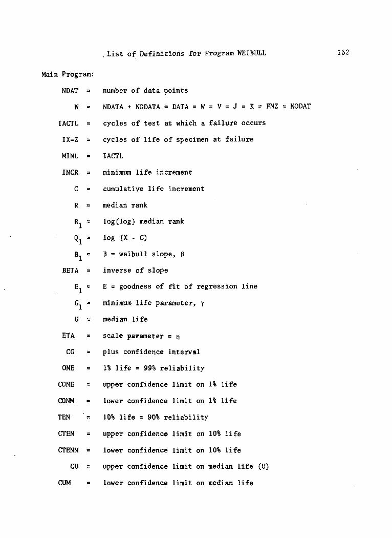
List of Definitions for Program WEIBULL 162

Main Program:

NDAT =

W =

IACTL =

IX=Z =

MINL =

INCR =

C =

R =

BETA =

U =

ETA =

CG

ONE

CONE

CONM «

TEN ' =

CTEN =

CTENM =

CU =

CUM

number of data points

NDATA + NODATA = DATA = W = V = J = K = F N Z = NODAT

cycles of test at which a failure occurs

cycles of life of specimen at failure

IACTL

minimum life increment

cumulative life increment

median rank

log (log) median rank

log (X - G)

B = weibull slope, B

inverse of slope

E = goodness of fit of regression line

minimum life parameter, y

median life

scale parameter = n

plus confidence interval

1% life = 99% reliability

upper confidence limit on 1% life

lower confidence limit on 1% life

10% life = 90% reliability

upper confidence limit on 10% life

lower confidence limit on 10% life

upper confidence limit on median life (U)

lower confidence limit on median life

CUMFREQ(I) =

PERCF(I)

DSTAT(I)

Subroutine

K

XMAX

XMIN

CSV

CEV

CLB

CUB

FREQ(J)

REQAREA(J) =

EXFREQ(J)

Subroutine for Kolmogorov-Smirnov Test

(Subroutine DTEST)

Weibull cumulative frequency distribution

cumulative observations (number of failures)

data cumulative frequency as percentage of failures

absolute difference between the data cumulative frequency

and the hypothesized cumulative frequency

for Chi-squared test (Subroutines CHISQA and CHISQB)

number of cells

largest value of cycles to failure

smallest value of cycles to failure

cell starting value

cell end value

cell lower bound

cell upper bound

number of observations in J cell

expected value of J cell (percentage)

expected number of observations

163

The program WEIBULL listing in Fortran language follows:

164

C—... WEIBULLC--—-WEIBULLc -WEIBULL

PROGKAM WEIBULL <INPUT,OUTPUT,TAPE2»INPUT»TAPE3aOUTPUT,

DIMENSION YUOO) ,FREQ(9) ,CLB(9) ,CU8(9) ,DSTAT(100) ,CUMFRQ (100) ,1 PERCF(IOO)

COMMON /N5/ IACTL. IX, Al, A2, NOR, A3* A4« AS, A6J » 0K a J). . __________ .............. _ . .....I a 0ICOUN » 0MOD... » Q .............. _______ ........ -XPREV «* 0«0RPREV a OtO

REWIND 5READ (2*10) NODAT, INCR»M_IF_IEUF.(2.J.) .83_ita _

10 FORMAT (40H - .216*18)80 IF (NODAT-50) 82,83,83 j82 WRITE _{3i40j ... . . . . _ . . . i40 FORMAT (SH1DATE.15X*9HRUN IDENT ) '.

WRITE (3*10) ;7 READ 12120)- IACTL t-IX-t AH- A2t NOR*~A3* A4* -AS* A6 •20 FORMAT (17, lX. 17, IX, 2A4, J3, 4A4, F16.6) j

IF (IX) 4, 3, g i2. J. a J * 1.. . I3 K a K * 1 !

I a I * 1 !y.(ix- a IACTL. — - -.. . ... . iIF (NOR) 6, 6, 5

to NOR a 15 NOD a NOD - * NOR _.._.. i

WRITE (4) IACTL, IX, Al, A2, NOR* A3* A4, AS* A6 i60 TO 7 i

ftIF (NODAT - NODI-.8, -9_».a ....._._ iM !..... EHROR STOP - NO. OF DATA NOT CORRECT j

8 WRITE (3*30) NODAT* NOD !30 FORMAT (22H1NO. OF DATA INCORRECT X1HO* 16, 5x» 16 / 1H1) i

REWIND 4 ._ _ ._ ;60 TO 83

9 REWIND 4WRITE <3*22Q) NQDAT* Jt_INro-M !

220 FORMAT (1HO*4X.11HNO. OF DATA I6,10X,13H NO. OF FAIL I6,10X*1I5H HZN LIFE INCR I6.5X.5H M « ,I6//) |WRITE, (3t230) ________ . . ________ _ - ....... - . .. !

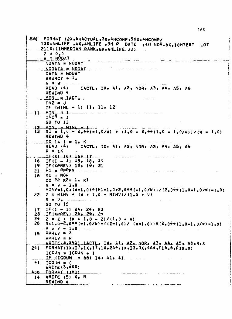
165

230 FORMAT (2X,6HACTUAL*3X**HCOMP,56x,4HCOMP/13X.4HLIFE ,4X,4HLIFE ,9H P DATE ,4H NOR.6X, 10HTEST LOT

Z * 0.0W a NOD AT ___ _"NOAJA » "NOD AT " """ .......... "~ ~NQDATA a NODAT ___ ..... - ... . ........ \DATA a NOOAT jAKURCY • 1.V .•_ tf. ...... _________________ _______ ... ':.READ (4) IACTL, IX, Alt A2, NOR» A3* A4, AS, A6 :REWIND 4 \

FNZ a J| IF (MINI. - 1) lli 11* 12j ..U-— MINL-J--J ------- -I INCR a 1i GO TO 13

MINL • 413 Rl a 1.0 - 2,*«(.1.0/W) * (1.0 - 2,»»<1.0 - 1.0/W))/(W - 1.0)

REWIND 4

READ (4) IACTL* IX* Al* A2> NOR* A3* A4, AS, A6X a IXIF(X) 16* 16* 17 _______ _____ ________ _____

16 IF(I - 1) 18* IS, 1919 IF(XPREV) 18* 18, 2121 &l-a-RpR£Y _____________ ... ______18 Kl s NOR

00 22 K2a 1, KlV g V • 1*0 ________________RINV«1,0*(W-1.0)«(R1-1.0*2.0»*(«1.0/W) )/(2.0»«(1.0-1.0/W)-1.0

22 Z a MINV * (W * 1.0 - RINV)/(1.0 * V)R a....O _____________ ____GO TO 15

17 IF(I - 1) 24, 24, 2323 ..JF.URREJa 26, 26t._2»24 z a L * <W * 1.0 - Z)/(1.0 * V)26 Ral.o-2.0<»«(-1.0/W)*( (Z-1,0)/ ( W-l .0 ) ) * ( 2.0»» ( 1 .0-1 . 0/W) -1 .0)

15 XPREV » xRPREV a R

____ WRIT£(3.241) IACTL, IX. Al. A2f MQPf A3. A4 . A5, A6.R.X241 FORMAT(lX»l7,lX»l7,lX,2A4,ix,I3,3Xt4A4,Fl6.6,F12.0)

14« .41 1- 4141 ICOUN a 0

WRITE(3,400)400 FORMAT14 WRITE (5) X, R

REWIND 4

166

5. . . . . . . . ... ' . ._ „_ _.El * 0.0I F ( Y ( 1 ) ,UE. 1000) GO TO 117IF tYUl iQTt 1000 -AND. Y t l ) tLF« Lfl6£0.} fiO... TO 1.16IF(Y(1) ,GT. 10000) INCR « 10000GO TO 127

116 JNCR =» rO-Q-0. . - —-60 TO 127

UJ INCR c 100

IF(M ,GT. 1000) M m M - 1000£1 jg.. 0 *~Q - -- -. _ _. .. _00 27 KNaM,MINL*INCRQSUM a 0*0RSUM a ..0.0 .. . ..-._QSOS a 0.0RSOS a 0.0

G » KN - IDO 28 I a lt K-R£AD- (5)IF(X) 28, 28* 29

29 IF(X - G) 31i 31« 32

:C— — NEGATIVE ARGUMENT IN LOG. FUNCTION

C— —100 FORMAT UHlt26HNEG. ARG. IN LOG. FUNCTION /.1H1)

GO TO 8332---04— «~AUM»-U--« -8) ------

IF(R) 31* 31, 34

£-<•»*»• - MEGA-T1-VE- ARGUMENT IH LOG FUNCTION

C --- —34 Rl= ALOG(ALOG(1 .0 / (1 .0 - R) ) )QSUM -* -Ql __________ .....

RSUM • RSUM * RlQSOS » QSOS * Ql * Ql

.. _____ RSOS--8-RS0S * Rl.jt_jaPROD » PROD * Ql « Rl

28 CONTINUE.. REMIND 5B » (FNZ • PROD • QSUM # RSUM)/(FNZ » QSOS - QSUM • QSUM)A • (RSUM - 8 • QSUM) / FNZ_£ ,J«_SQRI LLF.NZ- »..JISQS - QSUM. • QSUM).. • (FM2 « RSQS-* RSUM « RSUM)E - <FNZ«PROD - QSUM * RSUMJ/CIF(E - El) 37, 36, 36

36- El » E __ ._ ..... _____________ ..... _- . .. - -. -Gl « GBl « BAl

167

' 27 CONTINUE37 M a Q * 1 - INCR

38 ARG a EXP ( •BETA • 1.0/81EJA J8U » Gl * (0.69315«ARG)*«BETAONE « 61 * <0.01005«ARG)»«BETA

(Q.in5«AR6)«tfl£lA_ _B * Hi • (1.0 * 1.163 / SQRT(W» • - , « „ .CGaGl+.5»(U-Gl)<M4.32159«»<1.0/B)«0.074*«<l.O/B))/<W*»<l.O/B))

_ . _ . _FACT = CONST * 10.010038 • (0.995E-02»#BETA/B1 )C_ONE a ONE » FACT

CONM a ONE - FACTFACT • CONST • 3,1924.748 » (0,lQ436Q»»BETA/Bl)CTEN « TEN * FACTCTENM « TEN ->ACT

CU » U * FACTCUM * U - FACT

.-..WRITS (3,450) Rl, El, EJA-, &1.,C6. ONE+-CONE+-CONMWRITE (3i45i) TEN. CTEN, CTENM, U, CU, CUM

50 FORMAT (// 12X.13HWEI8ULL SLOPE,5X,15H800DNESS OF FIT ,5X,

213X,i2HMINIMUM LIFE ,11X»9HPLUS CONF,/35X.2F20.5,//

_-49X»lfeHONE PERCENT LIFE- Ulx«9HPLl!5 CONF • lOKt 10HMINUS CONF • /55X,3F20.5 //)

451 FORMAT (1H*,9X,16HTEN PERCENT LIFE,11X.9HPLUS CONF,10X,. 111H MINUS CONF ,/5X«3F20,5,//214X,11HMEOIAN LIFE »11X,9HPLUS CONF ,1QX, 10HMINUS CONF ,/35X.3F20.5 //)CALL DTEST (Y,BltGl>U.NQDATA,DSTAT,PERCF,CUMFRQ,ETAtSKSTAT)CALL CHISQA (Y,OATA,NOATA,PROB,AKURCY,XMEAN,DEV,Z,S1,B1,

1 XMAX,XMIN,CL8,CUB,NUMINTStCELLWO)CALL CHISQB (YCALL GRAPH (FREQ»XMAX,XMlN,CLB.CUB,SKSTATtCHlSQR,Bl,ETA,Gl.NDATA,

1 NUMJNTS.CELLWD)GO TQ 1 ____ ___ ___ ___ _____

83 CALL PLOT <0,0» 0.0* 999)CALL EXITEND __ _________

168

! SUBROUTINE DTEST <Y.B1»61tUtNQDATAtDSTAT»PERCF,CUMFRQtETA»SKSTAT)! DIMENSION Z(100) iY(lOO) iDSTATUOO) tPERCFUOO).CUMFRQ(100)ic!C SUBROUTINE TO CALCULATE THE KOLMOGOROV-SMIRNOW D-VALUESic

DO 5UO IsltNODATAZ(I) = 1.0 - EXP (-(((Y(I)-Gl)/ETA)*»8l))

500 CONTINUECC SET CUMFRQ(2) ARRAYC

DO 501 I=1»NODATA501 CUMFHQ(I) • I

C . - . .C PERCF = F(N) OF THE NUMBER OF DATAC

DO 502 .1 Hi. • NOD AT. A502 PERCF(I) a CUMFRQ(I)/NODATA

DO 503 IslfNODATA503 -OSTATIXJ-". Z<I> --PfiaCFU)

PRIMT 520PRINT 521t (DSTAT(I)ilal.NODATA)

521 FORMAT (&UUX«F10.5))520 FORMAT (//40X.53H D VALUES FOR KOLMOGOROV-SMIRNOV GOODNESS OF FIT

1TEST/41X,52H(LISTED IN THE SAME ORDER AS CYCLES.TO-FAILURE DATA)/)SKSTAT -a-4«0DO 10 laltNODATAIF(AdS(DSTAT(I)).GT.SKSTAT) SKSTAT * ABS(DSTAT(I))

10 CONTINUE-PRINT 400t SKSTAT

400 FORMAT(//f10Xt«KOLMOGOROV-SMIRNOV TEST RESULT * »»FS.5,/)RETUKNEND

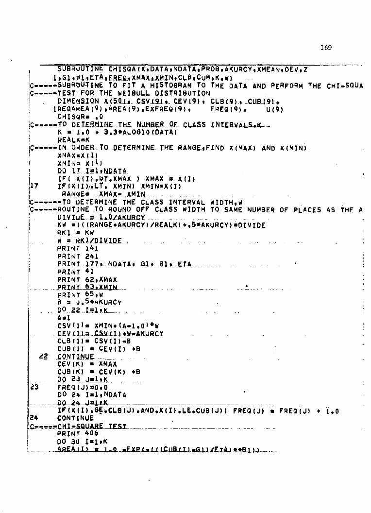
169

SU8R(JUTINL CHISQA(X»DATAiNDATAtPROStAKURCYiXMEANiOEVtZI l*aij_bL,ETAifRE£L.XMAX4-XM.INjCLB.tCu8|Jl4«))C—.—SUBROUTINE TO FIT A HISTOGRAM TO THE DATA AND PERFORM THE CHI-SQUA

-TEST FOR THE WEI8ULL DISTRIBUTIONDIMEfiSJQN X(5.Qlj_ CSVI9).i.. CEV(9) t CLB(9> • _CUE4-9U

1 R E Q A R E A ( 9 ) , A R E A ( 9 ) , E X F R E Q < 9 ) . FREQ(9 ) , U(9)CHlSURa .0

-----TO Q£l£R.fliNE. J£H£ NUMBER.. OF. CLASS INTERVALS**--K a 1.0 * 3.3«ALOG10(DATA)REALKaK

C——IN. OKD.ER.TQ .DETERMINE, THE RANGE.tFlND X.(MAXJ AND X(MIN)XMAX«X(1)

DO 17.J«.liNfiAlA.

17 lF(X(I)/iLf.*XMIN) XMINaX(I)RANyEa.XilAA-.XMIN

C——TO DETERMINE THE CLASS INTERVAL WIDTHSC— ROUTINE TO ROUND OFF CLASS *IDTH TO SAME NUMBER OF PLACES AS THE A

DI.VIME. a 1.0/AKURCY _ -KW a({(RANGE*AKURCY)/REALK)*.5*AKURCY)»DIVIDERK1 a KWW a HK1./DIVIDE _. - :PRINT 141PRINT 241 1PRl.NT--177-*--hUlATAt .G-U fll* ETA • !PRINT *1PRINT 62»XMAXPRINT 63tXMIN -.... :PRINT 65,wB a 0.5«MKURCY

. . HP.

CSV«I)» XMIN*<A-1.0>*W

CLB(I)* CSV(I)-BCUB (I) a CEV(I) *B

22 .CQWTlNUi ____CEV(K) « XMAXCUB(K) • CEV(K) *B

. _. DQ SJ.JL.I! ......23 FREQ(J)=0.0

DO 24 I«1|NOATA

IF(X(I) .GE.CLB(J) .AND.X(I) .LE.CUB(J) ) FREQ(J) a FREO(J) * 1.02* CONTINUEC—— CHI-SQUARE

PRINT 406DO 30 I»1»KAREA (I) c l,Q -EXP(»( ( (CUB (I )«Gl)/ETA) »»9l) )

170

IF (I ,EQ. 1) GO TO 51IF (i .GT. 1 .AND, I ,LT. K) 60 TO 52

- ._ .REQABEA (K-L-a- 1.0 .- AREA(K)GO TO 30

51 REQAKEA(I) a AREA(I)GO TO 30

52- - R£QA.HEA(n._a-AR.EA(I) -g A RE A (-1*1.) _______ . . . .30 CONTINUE76 DO 8U M = 1,K

FXFPgQ (M) aDATA»PEQAREA (M) ________________________ _ . . ' . . . .U (M) a ( ( EXFREU (M) -FREQ (M) ) »*2) /EXFR£Q (M)

60 CHISUR»CHISQR*U(M)C----«Jia.EHlN.T..IHE...TAflLE.ZQa_CJllaSaUAR£_J£SJ ........... ______88 00 33 I B 1,K

33 PRINT 34,I,CLB(I) ,CUB(I), EXFREQ < I ) ,FREQ < I ) tU < I)J=>RIfelT 35 1 CHISQR ________________________ .............

t>2 FORMAT ( lOXf 14HMAXIMUM VALUE«*F15.6)63 FORMAT ( 10X» HHMINIMUM VALUE«t Fl5.6)

Q X H A S S

FORMAT (1HO)406 FORMAT (8Xt5H CELL»10Xt 10HUOWER CELLt Ux» 10HUPPER CELL* 13X.8HEXPEC

213X, 8HBOUNDARY,13X.9HFRE<JUENCYtl2X,9HFREOUENCYil2X,13HVALUE OF CE3LL/)

, FORMAT (IQXt I2»SF21 .6) _________________ _________ ..... - - .......35 FORMAT (1HO t81X.25HTOTAL CHI-SQUARED VALUE ssF10.6//)141 FORMAT UHOi70X,»CHI«SQUARED TEST#,//)_24,l..F-ORMAT-UHOx70X-i»f:iX£D CEU. -hllOTHS**//) ____177 FORMAT (IHOt lOXt »INPUTS « »t!10i 3F15t3»X)78 CONTINUE

END

171

SUBROUTINE CHISQB (X»NDATA,G1*B1.ETA.CHISOR)DjMFNSIQM X(5p) t CUi{9J» CUB t9J-»- R E Q A REA-U J • AR£A(9>t FREQC5)«

2EXFREQ(9)t U(9)JC-—.SUBROUTINE TO FIT A HISTOGRAM TO THE DATA AND PERFORM THE|c-----CHt-SflUAaED_TESI-EOH. THE) PRINT 341

CHISUR a 0.0

00 26 Kw§»NOATA.5J 9 J+lIt.- tK--*LT-* MOAT - Ai C UB ( J ) •..( X < K ) *-X UU.L) 1/2 Q - - .....IF (K ,EQ. 5) CLB(J)»X(DIF (K .GTt 5 .AND. K .LT. NDATA) CUB (J)"CUB(J-l)

__ |_ a (NOATA»K) ...... - ........ ______ ..... _________ ~.IF(L.NE.O) AREA(J)«1.0-EXP(-(((CUB{J)-Ol)/ETA)»«Bl))IF(L.EQ.O) AREA(J) «1,0

..... FREQ( J)«5,Q ________ _ ___ , ____ ______ ..... ____IF(J.EQ.l) REQAREA(J)aAREA(J)IF(J.OT.l.ANO.L.NE.O) REQAREA ( J) .AREA ( J) -AREA ( J-l )IF (L.LT.5) -&O-T-OL27 _________ ......... -------------------GO TO 26

27 IF(L.NE.O) J«J*1_____ CIJH(J)«X(NDATA) ______________ ...... - ______ ..... _________ .....

REQAREA (J) *1.0. AREA (J-l )4» -« L-

26 CONTINUEI • J

._ DQ 2$ Jalt I

EXFRtQ(J) = NOATA«REQAREA(J)25 CONTINUE

K « X --.

62 I a 12420 IF (tXFREQ(I) .GE. 5.) GO TO 2430

- ..£XER£QU*-1) »-EXFREOC-I + I) * E.XFREO M)FREQ(I*1) * FREQ(I*1) * FREQ(I)J » I00 2»25 L=ltJEXFRtQ(L) - 0*

2425 FREQ(L) » 0.1 a 1*1GO TO 2420

2430 I a KIF (£XFREQ(I) ,6E. 5>) GO TO -2A5JJEXFRtQ(I-l) c EXFREQ(I-D«EXFREQ(I)FREQ(I-l) * FREOd-1) • FREQ(I)nn 2»45 igT.>fEXFRCQ(L) » 0.

.2445 F.REOIU s O.a

172

I .a00 TO 2440

2450 CONTINUEDO 95 M^ltKU(M) s 0.0IF (tXFREQ(M) .EQ. 0.) 60 TO 85U<M) •» ((EXFREQ(M) -• FREQ(M) )**2/EXFREQ(Mh

85

CHISQR • 0.000 90 Mal,K

9o ___ CHISQR « CHISQRJ » K

88 DO 3J I = IvJ33 ----- PRINT 34tUCLB(-U»CUB{X)t EXFg£q< 1)

PRINT 35t CHISQR34 FORMAT (10XtI2t5F2l.6)35

341 FORMAT(1HO»65X. "VARIABLE CELL WIDTHS*.//)78 CONTINUE__ RfTTUHN __ _ ____ _ ______________ .. ________

END

173

, . SUBRUUT INE. QRAPW (FREQiXMAX tXMI N • CLB-i CUfl*SKS • CHI SQR « BETA • ETA •1 1 GAMMA, NDATA,K,CELLWD)

DIMENSION FREQ<9) , CUB (9) ,CU8(9)INTEGER EQ-QT-134J >SUflJITL-l2)LOGICAL NITIALDATA NITIAL / .TRUE. /

; C _ _ . . - -1C READ PLOT CARD1C\ .8EA0.l2j.40Un IPLOT*-SUBT1JL*IPEN1 400 FORMAT (4A10)i I F (EOF(2 ) ) 999,3

3 IftIi»LQT»NE*7KMEIflULL) 00 TO 999IF(NITIAL) 4t5

* NITIAL a .FALSE.PEbL a 0.3 ...............IFdPEN .EQ. 10HBALL POINT) PEN • 0,0CALL INITIAL (0»ltPEN,0)

5 R£AO 4 .401) FOOT- . . _.. .........401 FORHAT(SAlO)

CC DETEKMINE DISTANCESC

2 XLENbTH = 6»0

H a 0.15YMAX a 0.0

IF(YMAX.LT.FREQd) ) YMAXsFREQ(I)1 CONTINUE

»- O+»0«NDATA --

IF(YMAX .GE. FRINL .AND. YMAX ,LT. FRINGE) GO TO 7IF(YMAX .GE. FRINGE) YMAX a IFIXtYMAX * FRINGE)

! GO TO 67 YMAX a IFIX(YMAX * FRINL)

. 6-CONIINUE. _IaYMAXIF((1/2*2).NE.I) YMAXaYMAX*!,XMIN » X_MIN_- 0.10 « (XMAX - XMIN)XDIF a XMAX - XMIN

CC DETERMINE. SCALING- F-ACTQRS

XSCALE a (XMAX - XMIN) / XLENGTH

E a IFIX(ALOG10(XMAX - XMIN))STP » 10.0 •« E

174

Cc LOCATE PLOTTER PEN:C

; CALL PLQJULENGTt^.tO»i"3)CALL PLOT<&.,-U.t-3)CA i i PLOT (O.tS.,.3)

175

|C .CONSTRUCT Y-AXIS

CALL PLOT <0.»YLENGTHt2>DXVmU/YSCALE

21 I F ( D I V . G E . ( 2 . » H ) ) GO TO 22D I V « 2 . » D I VGO TO 2.L. _______ . ._

22 STEP-DIVY Y « 0 .

23. CALL_P-LQT l.05,YY,3iCALL PLOT (- .05,YY,2)YNaYY«YSCALE

YY«YY*STEPIF(YY.LE.(YLEN6TH*.01M GO TO 23

IF (YY.LT.O.) YY«0,CALL SYMBOL (-04,YY,H,30HFREQUENCY/CLASS INTERVAL WIDTH,90,,30)

C CONSTRUCT* DRAW, AND LABEL X-AXISC

.._ -CALL PLOT- -10-.»0.43)XMINalFIX(XMlNXSTP)XMAX a IFIX(XMAX / STP * 1.0)XDIF rr XMAX - XMINXSCALE • XDIF / XLENGTH •• STPDIV"10,«XDIF/XLENGTHIF-lXJltN_*£Q-»JX«) GO TO 26CALL PLOT (.3*0.*2)CALL PLOT (.35,0.,3)

. . -CALL-P-LOT-(XLENQTH»Q.^) -CALL PLOT (.35,.05,3)CALL PLOT (.25,-.05,2)CALL-HLQ-T-U3*-. 05*3)CALL PLOT (.4,.05,2)GO TO 28

-26 CALL-PLOT (XLENQTH»0.,2)28 IF(DiV.LT.l2,7) 00 TO 30

.GO. TO -2830 DIV«OIV/10,

IF(OIV.LT.0.2) DIV«DIV*10.3? CALL NUMBER (0. ,-«2tH,Q. ,0 , ,0)

XX»o.DO 35 I "1.25

IF (XX.GT.XLENGTH) 40,33

176

33 CALL PLOT (XX*.b§t3)CALL PLOT (XX.-,05,2)XNsXMlN*I#XDIF/(DIV«XLENGTH)CALL NUMBER (XX-.l »-.2»HtXN»0. »0>

35 CONTINUE40 DO 41 I=l»2_ IF ( SUBTITL(I).EQ,1H ) QO TO »2

~4l CONTINUE

60 TO 4342 1=1-143 XXa4JU.ENGTH»I)/2.

CALL SYMBOL (XX, -.5, . l5, SUBTITL ( 1 ) » 0. t I )JECSlP-^Lia.Ol) GO T.Q-APCALL WHE^E (XX , YY, IFAKE)CALL SYMBOL (XX»- .5»H»5H X 10*0. *5)

.. .CALL-ttHEHE (JUU.YY, IFAK&) . . ..CALL NUMBER (XX*H, YY+.5«h, ,5*H,E.O. ,-1 )

CC ....... COM3 TBUCJ_.. AND. QRAM..H1SJ10.QBAM .....C

48 DO SO I»1»KCLB Ul ?_tiCLB-a )V S.T.PJ -XM I N 1 /.( X SC ALE/S.TP-4

50 CUB( I )» ( (CUB( I ) /STP) -XMIN) / (XSCALE/STP)52 CALL PLOT (CLB ( 1 ) ,0. .3)

qO .5 - J.altK .......... _______ .......Y»FREQ(I)/YSCALECALL PLOT (CLB(I)»Y»2)CALL PLQT._ (CUB U),Y».2X~

54 CALL PLOT (CUB(I),0.,2)55 CONTINUE

.C ______ _ .......... ____ .......... ______C COMPUTE AND DRAW NORMAL CURVE ONE POINT AT A TIMEC

..6.O.. SIEP_i..XDJf ».STB_XX » XMIN « STPCALL PLOT(0.tO.,3). _ _ _ _ _ _ _ _ _ _ _ _ _ _ _ _ _ _ _ _ _ _ _ . . . . . _ _ _ _ _ _ _ _ _ _ _CHK • EXP(-l.O)IF (BETA ,LT. 1.0) YSCALEPYSCALE«EACT/CHKSL «._8EtA. _ ETA. .___ _. __________IDOIT • 2HNO00 100 I a 1,150IF (GAMMA .GT. XX) GO TO 100 ____________ _ ...... _ ___ _ .Z » (XX - GAMMA) / ETAY » BE • 2 •» (BETA - 1.0) • EXP ( - 1.0 * Z •• BETA)

177

_Y_ » Y i_ Y SCALE • NDATA * CELLED." XU"(XX«.XMIN«STP)/XSCALEIFdUOIT .EQ. 2HNO) GO TO 90IFUU.GT.20.) QO TO 100IF(XMZN.EQtO.) 80,70

TO IF(XU.GE.O.*) BOt'o80 CALL PLOT (XU.V.2)

GO TO 10090 CALL PLOT (XU,Y,3). 1DO_LI_ .» _3H.Y_ES ... _

100 XX»XX*ST£PCC. _QIHE8_. ALPHA-NUMERICC

130 CALL PLOT(0.t*l.f-3)CALLCALL

COMMENTARY

SYMBOL (0.0*O.OtH,24HKOLMOGOROV-SMIRNOVWHERE <xxa YY« IFAKEI . _.._

TEST!,0.0,24)

CALL SYMBOL <0.0,-2,0*H,H,17HCHI-SQUARED TESTJ,0.0,17)

CALL SYMBOL (0.0 ,-6.0«H,H,21HMIMMUM LIFE (GAMMA) t ,6. 0*21)CALL SYMBOL (0.0,-8.0*«»Hf22HSCALE PARAMETER (ETA)I,0.0,22)CAU.-blUMa£fi-4XX»0»0*H^SKS»A»0-f3). .CALL NUMBER (XX,-2.0»H,H,CHlSQR,o.O,3)CALL NUMBER (XX»-4.0*H»HfBETA»0.0»3)

CALL NUMBER (XX»*-8.0«H9H9ETA90.0 ,-1)CALL SYMBOL(0.,-14.»H,H,FOOT(l),o.»50)C&LL SYMBQL (0. t-^.^HtHtFOOT (6) «0« *50)CALL SYMBOLIC.»-18.*H,H,FOOT(ll).O.tSfl)CALL SYMBOL(0.,-20.*H,H,FOOT(16),0,,50)CALL_iYMflQL4X)-. , "22. tH Ji FIM) T(21) ,0.,50)CALL SYMBOL(0.,»24.«H,H,FOOT(26),0.,50)XXa(xLENGTH-3.75)/2.

CALL SYMBOL (XX,6.25,H,3lHwEIBULL DISTRIBUTION PARAMETERS,0.0,31)999 RETUHN

. -END

APPENDIX E

POP PROGRAM TO CALCULATE ENDURANCE STRENGTHPARAMETERS FROM STAIRCASE TESTS

C-FOCAL, 1969

01.10 A "MINIMUM STRESS LEVEL", YP, !01.20 A "STRESS INCREMENT", DP, !01.30 A "NO OF SPECIMENS", NS, !01.40 T "IF TEST IS BASED ON FAILURES THE CODE IS 0", !01.50 T "IF BASED ON SUCCESSES THE CODE IS 1", !01.60 A "WHAT IS THE CODE?", Co, !01.70 A "NO OF STRESS LEVELS IN TEST", I, !, !01.74 S CD - 001.75 S A e o01.76 S B « 001.77 T "NO OF SPEC IN EACH LEVL STARTING FROM THE 2ND LOWEST", !01.80 FOR J = 1, 1, 1-1; DO 4.0

02.10 S SD = 1.62*DP*((NS*B-A+2)/NS 2+0.029)02.20 IF (CO) 2.3,2.3,2.402.30 S MU = YP+DP*(A/NS-.5)02.35 GOTO 2.702.40 S MU = YP+DP*(A/NS-.5)02.70 T %10.03 "MEAN", MU, !, "STD DEV", SD, !02.80 Q

04.10 A NI, •04.20 S CU = CU+104.30 S A = A+CU*NI04.40 S B = B+CU 2*NI

APPENDIX F

PDF PROGRAM TO CALCULATE PAN WEIGHTS FOR DESIRED BENDING 179

STRESS LEVELS FOR THE ANN ARBOR RESEARCH MACHINE

C-FOCAL, 1969

01.10 A "DIAMETER, D, !01.11 A "LOWER STRESS", A, !01.12 A "UPPER STRESS", B, !01.13 A "INCREMENT", I, !01.15 T "STRESS LEVEL"," MOMENT"," PAN LOAD", I01.20 F ST=A, I, B,; DO 2.0

02.20 S M=3.1416*D+3*ST/3202.30 S P=((M+0.267)/4.07)-8.62502.40 T %8.40," ",ST," ",M," ",P,l

0.350 GOTO 1.10*

180

REPORT DISTRIBUTION LIST

GRANT NCR 03-002-044

Copies

National Aeronautics § Space AdministrationLewis Research Center21000 Brookpark RoadCleveland, Ohio 44135Attn: J. H. Childs, MS 3-3 1

H. W. Plohr, MS 54-1 1P. A. Thollot, MS 54-4 1H. A. Shumaker, MS 54-4 1N. T. Musial, MS 500-311 1G. Mandel, MS 6-2 1Librarian, MS 60-3 2Report Control Office, MS 5-5 1V. F. Hlavin, MS 3-14 1Technology Utilization Office, MS 3-19 1W. F. Darikhoff, MS 500-111 1V. R. Lalli, MS 54-4 3F. H. Stickney, MS 500-203 1C. R. Ensign, MS 49-1 1J. P. Gyekenyesi, MS 21-4 1

National Aeronautics and Space AdministrationScientific and Technical Information FacilityCollege Park, Maryland 20740 3

plus reproducible

US Air Force Aeropropulsion LaboratoryWright Patterson AFBDayton, Ohio 45433Attn: Library 1

U.S. Army R § D LaboratoryFt. Belvoir, Virginia 22060Attn: Library 1

Office of Naval ResearchArlington, Virginia 22217Attn: Mr. M. K. Ellingsworth C473 1

Library 1

National Science Foundation1800 G. Street, NWWashington, D.C. 20550Attn: Dr. Michael Gaus, RM 340 1

Library 1

181

REPORT DISTRIBUTION LIST

GRANT NCR 03-002-044

Copies

U. S. Atomic Energy CommissionTechnical Reports LibraryWashington, D. C. 20545 1

NASA Langley Research CenterLangley StationHampton, Va. 23365Attn: Library 1

NASA Manned Spacecraft CenterHouston, Texas 77001Attn: Library 1

NASA Manned Space Flight CenterHuntsville, Ala. 35812Attn: Library 1

U.S. Atomic Energy CommissionTechnical Information Service

ExtensionP. 0. Box 62Oak Ridge, Tenn. 37830 3

National Aeronautics and Space AdministrationNASA Headquarters Program OfficeWashington, D. C. 20546Attn: KR/D. E. Negola 1

RNP/F. Scholman 1Y/F. B. Smith 1

NASA Ames Research CenterAmes Research CenterMoffett Field, California 94035Attn: Library 1

NASA Flight Research CenterFlight Research CenterP. 0. Box 273Edwards, California 93523Attn: Library 1

182

REPORT DISTRIBUTION LIST

GRANT NCR 03-002-044

Copies

NASA Goddard Space Flight CenterGoddard Space Flight CenterGreenbelt, Md. 20771Attn: Library

Jet Propulsion Laboratory4800 Oak Groove DrivePasadena, California 91103Attn: Library

DirectorResearch and DevelopmentU.S. Array Weapons CommandRock Island Arsenal, Illinois 61201Attn: Dr. E. Haug

Dr. M. S. OjalvoDivision of EngineeringNational Science Foundation1800 G. Street, NWWashington, D. C. 20550

Dr. Walter J. Fahey. DeanCollege of EngineeringUniversity of ArizonaTucson, Arizona 85721

Dr. George W. Howard, DirectorEngineering Experiment StationCollege of EngineeringUniversity of ArizonaTucson, Arizona 85721

Dr. Lawrence B. Scott, HeadAerospace and Mechanical Engineering DepartmentUniversity of ArizonaTucson, Arizona 85721

Louie B. ChesterAerospace and Mechanical Engineering DepartmentUniversity of ArizonaTucson, Arizona 85721

183

REPORT DISTRIBUTION LIST

GRANT NCR 03-002-044

Copies

Dr. Dimitri B. KececiogluAerospace and Mechanical Engineering DepartmentUniversity of ArizonaTucson, Arizona 85721