Embed Size (px)
Citation preview

Dr. Mahmoud M. Al-Husari
Modern Control SystemsLecture Notes
This set of lecture notes are never to be considered as a substituteto the textbook recommended by the lecturer.

ii
Contents
1 Linear Systems 11.1 Introduction . . . . . . . . . . . . . . . . . . . . . . . . . . . . . . 11.2 Review of System Modeling . . . . . . . . . . . . . . . . . . . . . 21.3 State-variable Modeling . . . . . . . . . . . . . . . . . . . . . . . 6
1.3.1 The Concept of State . . . . . . . . . . . . . . . . . . . . 81.4 Simulation Diagrams . . . . . . . . . . . . . . . . . . . . . . . . . 9
1.4.1 State-variable models from Transfer Function . . . . . . . 101.4.2 Transfer Functions from State-variable Models . . . . . . 15
1.5 System Interconnections . . . . . . . . . . . . . . . . . . . . . . . 171.5.1 Series and Parallel Connections . . . . . . . . . . . . . . . 171.5.2 Feedback Connection . . . . . . . . . . . . . . . . . . . . . 17
1.6 Solution of State Equations . . . . . . . . . . . . . . . . . . . . . 181.6.1 Properties of the State-Transition Matrix . . . . . . . . . 22
1.7 Characteristic Equations . . . . . . . . . . . . . . . . . . . . . . . 241.7.1 Eigenvalues . . . . . . . . . . . . . . . . . . . . . . . . . . 251.7.2 Eigenvectors . . . . . . . . . . . . . . . . . . . . . . . . . 25
1.8 Similarity Transformation . . . . . . . . . . . . . . . . . . . . . . 271.8.1 Properties of the Similarity Transformation . . . . . . . . 291.8.2 Diagonal Canonical Form . . . . . . . . . . . . . . . . . . 291.8.3 Control Canonical Form . . . . . . . . . . . . . . . . . . . 311.8.4 Observer Canonical Form . . . . . . . . . . . . . . . . . . 33
2 Controllability and Observability 372.1 Motivation Examples . . . . . . . . . . . . . . . . . . . . . . . . 372.2 Controllability . . . . . . . . . . . . . . . . . . . . . . . . . . . . 39
2.2.1 Controllability Tests . . . . . . . . . . . . . . . . . . . . . 402.3 Observability . . . . . . . . . . . . . . . . . . . . . . . . . . . . . 41
2.3.1 Observability Tests . . . . . . . . . . . . . . . . . . . . . . 422.4 Frequency Domain Tests . . . . . . . . . . . . . . . . . . . . . . . 432.5 Similarity Transformations Again . . . . . . . . . . . . . . . . . . 46
3 Stability 473.1 Introduction . . . . . . . . . . . . . . . . . . . . . . . . . . . . . . 473.2 Stability Definitions . . . . . . . . . . . . . . . . . . . . . . . . . 48
iii
iv CONTENTS
4 Modern Control Design 514.1 State feedback . . . . . . . . . . . . . . . . . . . . . . . . . . . . 514.2 Pole-Placement Design . . . . . . . . . . . . . . . . . . . . . . . . 524.3 Missing Notes . . . . . . . . . . . . . . . . . . . . . . . . . . . . . 544.4 State Estimation . . . . . . . . . . . . . . . . . . . . . . . . . . . 54
4.4.1 Estimator Design . . . . . . . . . . . . . . . . . . . . . . . 574.5 Closed-Loop System Characteristics . . . . . . . . . . . . . . . . 58
4.5.1 Controller-Estimator Transfer Function . . . . . . . . . . 604.6 Reduced-order State Estimators . . . . . . . . . . . . . . . . . . . 61
4.6.1 Example page 263 . . . . . . . . . . . . . . . . . . . . . . 654.7 Systems with Inputs . . . . . . . . . . . . . . . . . . . . . . . . . 65
4.7.1 Full State Feedback . . . . . . . . . . . . . . . . . . . . . 65
Chapter 1Linear Systems
1.1 Introduction
Control theory can be approached from a number of directions. The firstsystematic method of dealing with what is now called control theory beganto emerge in the 1930s. Transfer functions and frequency domain techniquesdominated the so called classical approaches to control theory. In the late 1950sand early 1960s a time domain approach using state variable descriptions startedto emerge. The 1980s saw great advances in control theory for the robust designof systems with uncertainties in their dynamic characteristics. The concepts ofH∞ control and µ-synthesis theory were introduced.
For a number of years the state variable approach was synonymous withmodern control theory. At the present time state variable approach and thevarious transfer function based methods are considered on an equal level, andnicely complement each other. This course is concerned with the analysis anddesign of control systems with the state variable point of view. The class ofsystems studied are assumed linear time-invariant (LTI) systems.
Linear time-invariant systems are usually mathematically described in one oftwo domains: time-domain and frequency-domain. In time-domain, the system’srepresentation is in the form of a differential equation. The frequency domainapproach usually results in a system representation in the form of a transferfunction. By use of the Laplace transform the transfer function can be derivedfrom the differential equations, and a differential equation model can be derivedfrom the the transfer function using the inverse Laplace transform. A transferfunction can be writtten only for the case in which the system model is a lineartime-invariant differential equation and the system initial conditions are ignored.
It is assumed that the student is familiar with obtaining the mathematicalmodels of various physical systems in the form of differential equations andtransfer functions. Knowledge of the laws of physics for mechanical, rotationalmechanical, and electrical systems is also assumed to be familiar to the student.
1
2 CHAPTER 1. LINEAR SYSTEMS
1.2 Review of System Modeling
In this section we briefly review obtaining mathematical models of physi-cal systems by means of several examples.. By the term mathematical modelwe mean the mathematical relationships that relate the output of a system toits input. Such models can be constructed from the knowledge of the physicalcharacteristics of the system, i.e. mass for a mechanical system or resistance foran electrical system.
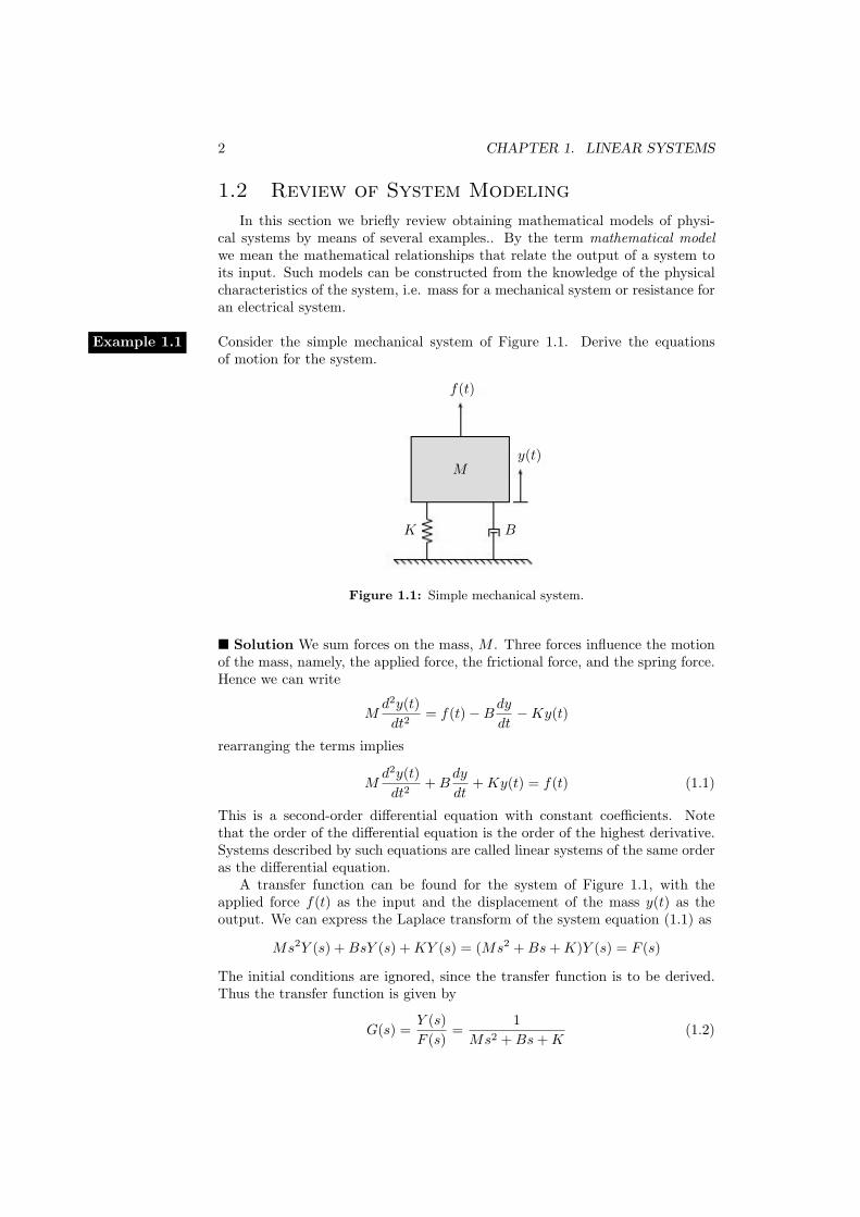
Consider the simple mechanical system of Figure 1.1. Derive the equationsExample 1.1of motion for the system.
f(t)
My(t)
K B
Figure 1.1: Simple mechanical system.
� Solution We sum forces on the mass, M . Three forces influence the motionof the mass, namely, the applied force, the frictional force, and the spring force.Hence we can write
Md2y(t)dt2
= f(t)−Bdydt−Ky(t)
rearranging the terms implies
Md2y(t)dt2
+Bdy
dt+Ky(t) = f(t) (1.1)
This is a second-order differential equation with constant coefficients. Notethat the order of the differential equation is the order of the highest derivative.Systems described by such equations are called linear systems of the same orderas the differential equation.
A transfer function can be found for the system of Figure 1.1, with theapplied force f(t) as the input and the displacement of the mass y(t) as theoutput. We can express the Laplace transform of the system equation (1.1) as
Ms2Y (s) +BsY (s) +KY (s) = (Ms2 +Bs+K)Y (s) = F (s)
The initial conditions are ignored, since the transfer function is to be derived.Thus the transfer function is given by
G(s) =Y (s)F (s)
=1
Ms2 +Bs+K(1.2)
1.2. REVIEW OF SYSTEM MODELING 3
Transfer functions represent the ratio of a system’s frequency domain output tothe frequency domain input, assuming that the initial conditions on the systemare zero. �
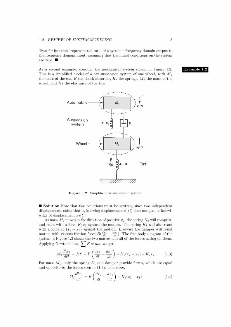
As a second example, consider the mechanical system shown in Figure 1.2. Example 1.2This is a simplified model of a car suspension system of one wheel, with M1
the mass of the car, B the shock absorber, K1 the springs, M2 the mass of thewheel, and K2 the elastance of the tire.
Figure 1.2: Simplified car suspension system.
� Solution Note that two equations must be written, since two independentdisplacements exist; that is, knowing displacement x1(t) does not give us knowl-wdge of displacement x2(t).
As massM2 moves in the direction of positive x2, the springK2 will compressand react with a force K2x2 against the motion. The spring K1 will also reactwith a force K1(x2 − x1) against the motion. Likewise the damper will resistmotion with viscous friction force B(dx2
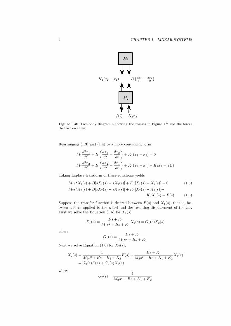
dt −dx1dt ). The free-body diagram of the
system in Figure 1.3 shows the two masses and all of the forces acting on them.Applying Newton’s law,
∑F = ma, we get
M2d2x2
dt2= f(t)−B
(dx2
dt− dx1
dt
)−K1(x2 − x1)−K2x2 (1.3)
For mass M1, only the spring K1 and damper provide forces, which are equaland opposite to the forces seen in (1.3). Therefore,
M1d2x1
dt2= B
(dx2
dt− dx1
dt
)+K1(x2 − x1) (1.4)
4 CHAPTER 1. LINEAR SYSTEMS
K1(x2 − x1) B(dx2dt −
dx1dt
)M1
M2
f(t) K2x2
Figure 1.3: Free-body diagram s showing the masses in Figure 1.2 and the forcesthat act on them.
Rearranging (1.3) and (1.4) to a more convenient form,
M1d2x1
dt2+B
(dx1
dt− dx2
dt
)+K1(x1 − x2) = 0
M2d2x2
dt2+B
(dx2
dt− dx1
dt
)+K1(x2 − x1)−K2x2 = f(t)
Taking Laplace transform of these equations yields
M1s2X1(s) +B[sX1(s)− sX2(s)] +K1[X1(s)−X2(s)] = 0 (1.5)
M2s2X2(s) +B[sX2(s)− sX1(s)] +K1[X2(s)−X1(s)]+
K2X2(s) = F (s) (1.6)
Suppose the transfer function is desired between F (s) and X1(s), that is, be-tween a force applied to the wheel and the resulting displacement of the car.First we solve the Equation (1.5) for X1(s),
X1(s) =Bs+K1
M1s2 +Bs+K1X2(s) = G1(s)X2(s)
whereG1(s) =
Bs+K1
M1s2 +Bs+K1
Next we solve Equation (1.6) for X2(s),
X2(s) =1
M2s2 +Bs+K1 +K2F (s) +
Bs+K1
M2s2 +Bs+K1 +K2X1(s)
= G2(s)F (s) +G3(s)X1(s)
whereG2(s) =
1M2s2 +Bs+K1 +K2
1.2. REVIEW OF SYSTEM MODELING 5
andG3(s) =
Bs+K1
M2s2 +Bs+K1 +K2
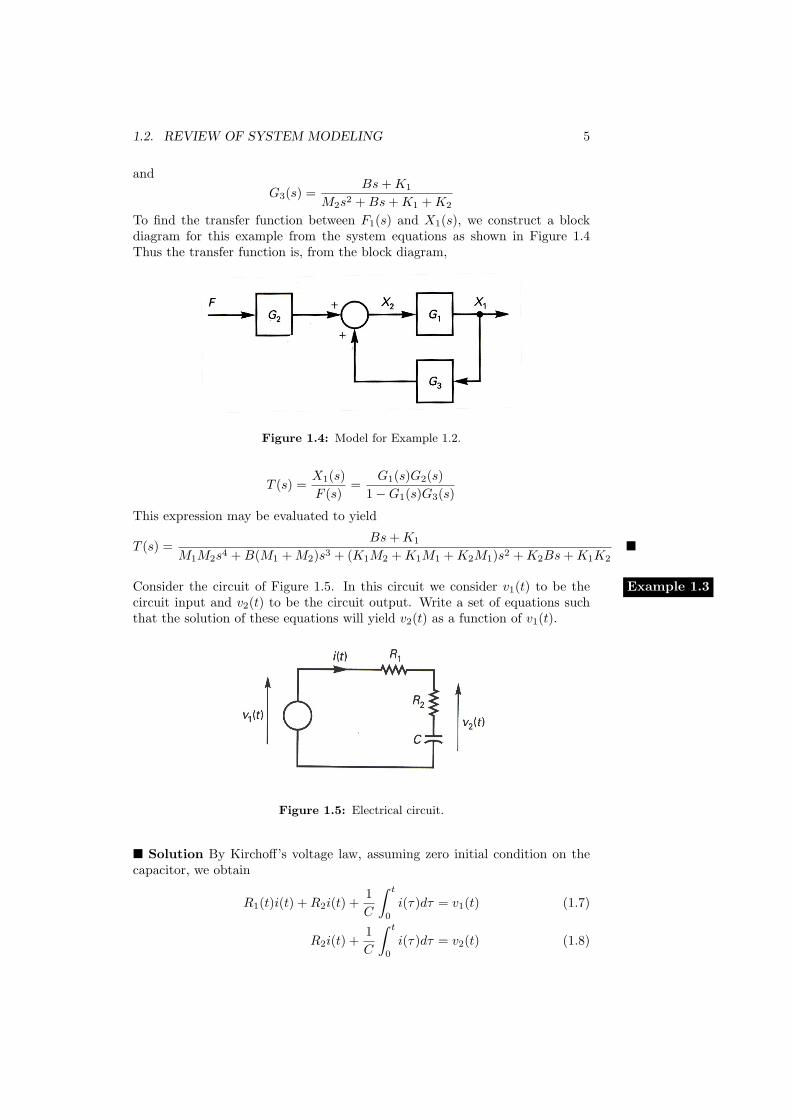
To find the transfer function between F1(s) and X1(s), we construct a blockdiagram for this example from the system equations as shown in Figure 1.4Thus the transfer function is, from the block diagram,
Figure 1.4: Model for Example 1.2.
T (s) =X1(s)F (s)
=G1(s)G2(s)
1−G1(s)G3(s)
This expression may be evaluated to yield
T (s) =Bs+K1
M1M2s4 +B(M1 +M2)s3 + (K1M2 +K1M1 +K2M1)s2 +K2Bs+K1K2�
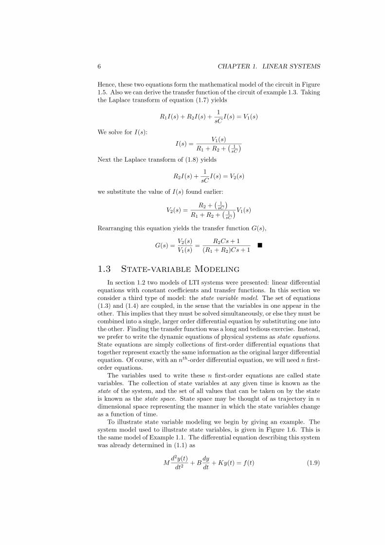
Consider the circuit of Figure 1.5. In this circuit we consider v1(t) to be the Example 1.3circuit input and v2(t) to be the circuit output. Write a set of equations suchthat the solution of these equations will yield v2(t) as a function of v1(t).
Figure 1.5: Electrical circuit.
� Solution By Kirchoff’s voltage law, assuming zero initial condition on thecapacitor, we obtain
R1(t)i(t) +R2i(t) +1C
∫ t
0
i(τ)dτ = v1(t) (1.7)
R2i(t) +1C
∫ t
0
i(τ)dτ = v2(t) (1.8)
6 CHAPTER 1. LINEAR SYSTEMS
Hence, these two equations form the mathematical model of the circuit in Figure1.5. Also we can derive the transfer function of the circuit of example 1.3. Takingthe Laplace transform of equation (1.7) yields
R1I(s) +R2I(s) +1sC
I(s) = V1(s)
We solve for I(s):
I(s) =V1(s)
R1 +R2 +(
1sC
)Next the Laplace transform of (1.8) yields
R2I(s) +1sC
I(s) = V2(s)
we substitute the value of I(s) found earlier:
V2(s) =R2 +
(1sC
)R1 +R2 +
(1sC
)V1(s)
Rearranging this equation yields the transfer function G(s),
G(s) =V2(s)V1(s)
=R2Cs+ 1
(R1 +R2)Cs+ 1�
1.3 State-variable Modeling
In section 1.2 two models of LTI systems were presented: linear differentialequations with constant coefficients and transfer functions. In this section weconsider a third type of model: the state variable model. The set of equations(1.3) and (1.4) are coupled, in the sense that the variables in one appear in theother. This implies that they must be solved simultaneously, or else they must becombined into a single, larger order differential equation by substituting one intothe other. Finding the transfer function was a long and tedious exercise. Instead,we prefer to write the dynamic equations of physical systems as state equations.State equations are simply collections of first-order differential equations thattogether represent exactly the same information as the original larger differentialequation. Of course, with an nth-order differential equation, we will need n first-order equations.
The variables used to write these n first-order equations are called statevariables. The collection of state variables at any given time is known as thestate of the system, and the set of all values that can be taken on by the stateis known as the state space. State space may be thought of as trajectory in ndimensional space representing the manner in which the state variables changeas a function of time.
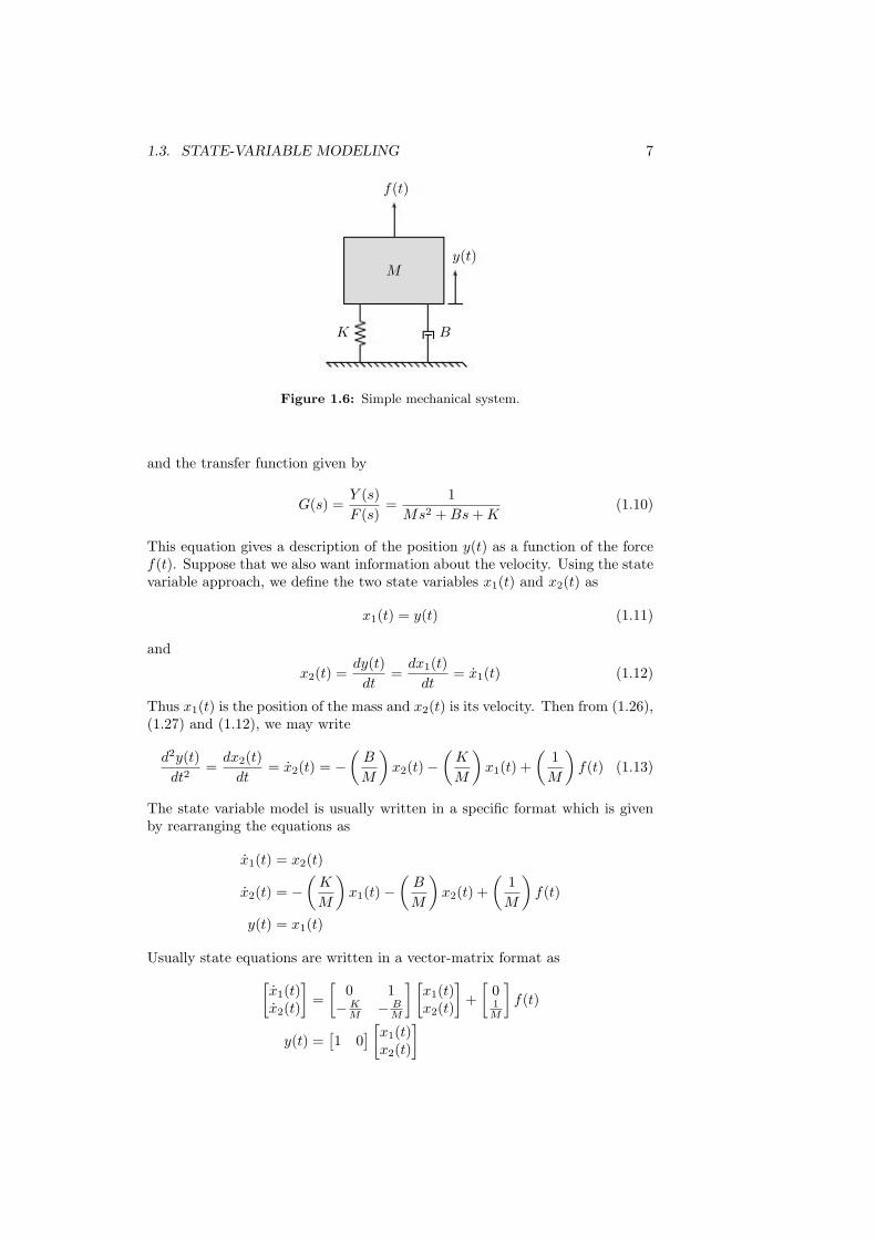
To illustrate state variable modeling we begin by giving an example. Thesystem model used to illustrate state variables, is given in Figure 1.6. This isthe same model of Example 1.1. The differential equation describing this systemwas already determined in (1.1) as
Md2y(t)dt2
+Bdy
dt+Ky(t) = f(t) (1.9)
1.3. STATE-VARIABLE MODELING 7
f(t)
My(t)
K B
Figure 1.6: Simple mechanical system.
and the transfer function given by
G(s) =Y (s)F (s)
=1
Ms2 +Bs+K(1.10)
This equation gives a description of the position y(t) as a function of the forcef(t). Suppose that we also want information about the velocity. Using the statevariable approach, we define the two state variables x1(t) and x2(t) as
x1(t) = y(t) (1.11)
and
x2(t) =dy(t)dt
=dx1(t)dt
= x1(t) (1.12)
Thus x1(t) is the position of the mass and x2(t) is its velocity. Then from (1.26),(1.27) and (1.12), we may write
d2y(t)dt2
=dx2(t)dt
= x2(t) = −(B
M
)x2(t)−
(K
M
)x1(t) +
(1M
)f(t) (1.13)
The state variable model is usually written in a specific format which is givenby rearranging the equations as
x1(t) = x2(t)
x2(t) = −(K
M
)x1(t)−
(B
M
)x2(t) +
(1M
)f(t)
y(t) = x1(t)
Usually state equations are written in a vector-matrix format as[x1(t)x2(t)
]=[
0 1−KM − B
M
] [x1(t)x2(t)
]+[
01M
]f(t)
y(t) =[1 0
] [x1(t)x2(t)
]
8 CHAPTER 1. LINEAR SYSTEMS
1.3.1 The Concept of State
The concept of state occupies a central position in modern control theory. Itis a complete smmary of the status of the system at a particular point in timeand is defined as:
Definition The state of a system at any time t0 is the amount of informa-tion at t0 that, together with all inputs for t ≥ t0, uniquely determines thebehaviour of the system for all t ≥ t0.
Knowledge of the state at some initial time t0, plus knowledge of the systeminputs after t0, allows the determination of the state at a later time t1. Asfar as the state at t1 is concerned, it makes no difference how the initial statewas attained. Thus the state at t0 constitutes a complete history of the systembehaviour prior to t0.
The most general state space representation of a LTI system is given by
x(t) = Ax(t) + Bu(t) (1.14)y(t) = Cx(t) + Du(t) (1.15)
where
x(t) = state vector = (n× 1) vector of the states of an nth-order systemA = (n× n) system matrixB = (n× r) input matrix
u(t) = input vector = (r × 1) vector composed of the system input functionsy(t) = output vector = (p× 1) vector composed of the defined outputs
C = (p× n) output matrixD = (p× r) matrix to represent direct coupling between input and output
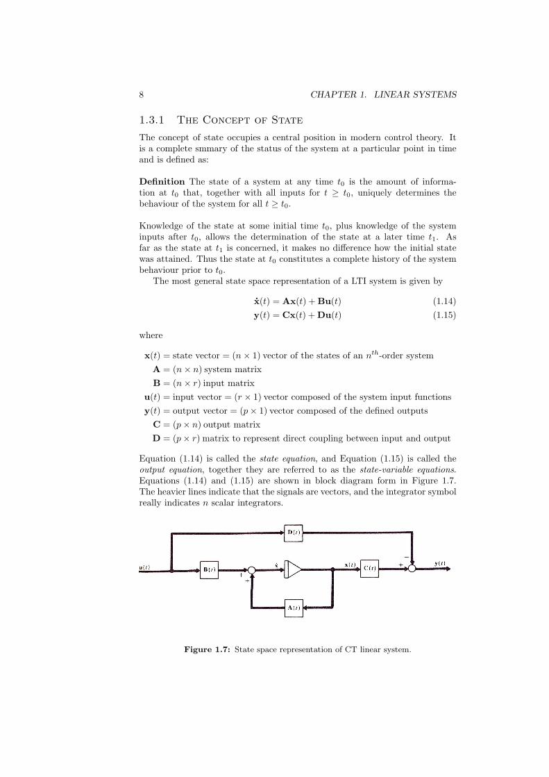
Equation (1.14) is called the state equation, and Equation (1.15) is called theoutput equation, together they are referred to as the state-variable equations.Equations (1.14) and (1.15) are shown in block diagram form in Figure 1.7.The heavier lines indicate that the signals are vectors, and the integrator symbolreally indicates n scalar integrators.
Figure 1.7: State space representation of CT linear system.
1.4. SIMULATION DIAGRAMS 9
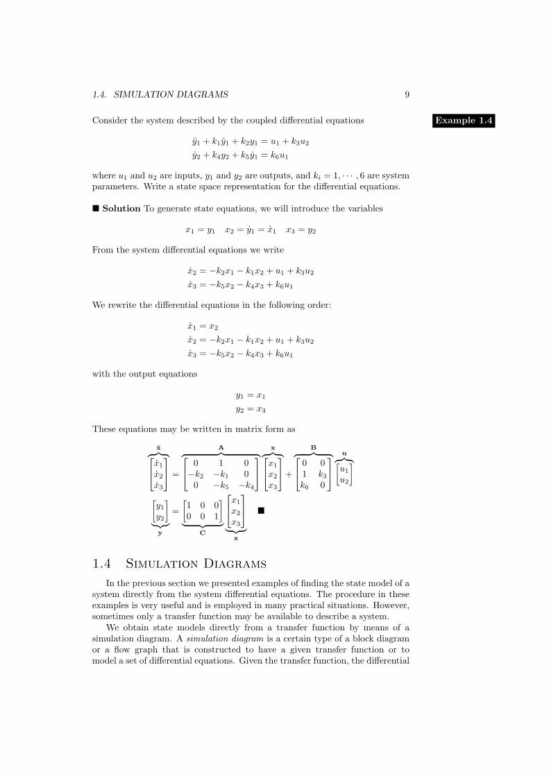
Consider the system described by the coupled differential equations Example 1.4
y1 + k1y1 + k2y1 = u1 + k3u2
y2 + k4y2 + k5y1 = k6u1
where u1 and u2 are inputs, y1 and y2 are outputs, and ki = 1, · · · , 6 are systemparameters. Write a state space representation for the differential equations.
� Solution To generate state equations, we will introduce the variables
x1 = y1 x2 = y1 = x1 x3 = y2
From the system differential equations we write
x2 = −k2x1 − k1x2 + u1 + k3u2
x3 = −k5x2 − k4x3 + k6u1
We rewrite the differential equations in the following order:
x1 = x2
x2 = −k2x1 − k1x2 + u1 + k3u2
x3 = −k5x2 − k4x3 + k6u1
with the output equations
y1 = x1
y2 = x3
These equations may be written in matrix form as
x︷ ︸︸ ︷x1
x2
x3
=
A︷ ︸︸ ︷ 0 1 0−k2 −k1 0
0 −k5 −k4
x︷ ︸︸ ︷x1
x2
x3
+
B︷ ︸︸ ︷ 0 01 k3
k6 0
u︷ ︸︸ ︷[u1
u2
][y1y2
]︸︷︷︸
y
=[1 0 00 0 1
]︸ ︷︷ ︸
C
x1
x2
x3
︸ ︷︷ ︸
x
�
1.4 Simulation Diagrams
In the previous section we presented examples of finding the state model of asystem directly from the system differential equations. The procedure in theseexamples is very useful and is employed in many practical situations. However,sometimes only a transfer function may be available to describe a system.
We obtain state models directly from a transfer function by means of asimulation diagram. A simulation diagram is a certain type of a block diagramor a flow graph that is constructed to have a given transfer function or tomodel a set of differential equations. Given the transfer function, the differential
10 CHAPTER 1. LINEAR SYSTEMS
equations, or the state equations of a system, we can construct a simulationdiagram of the system.
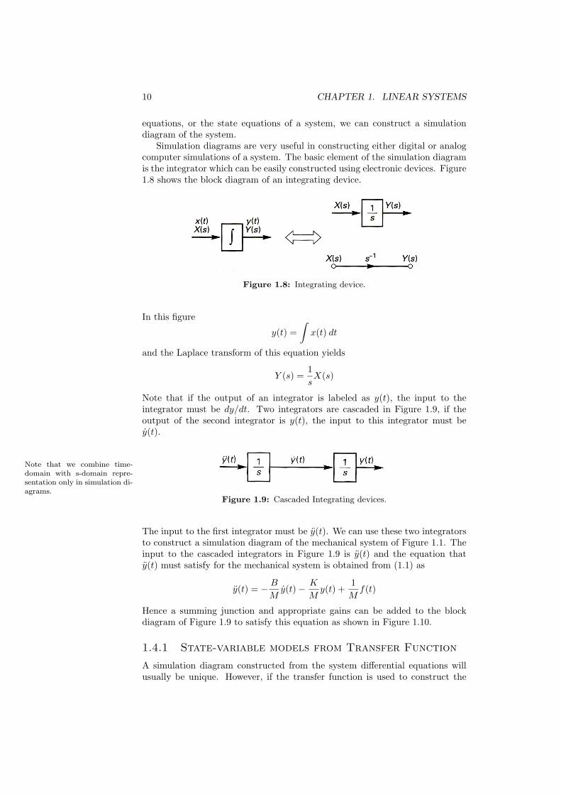
Simulation diagrams are very useful in constructing either digital or analogcomputer simulations of a system. The basic element of the simulation diagramis the integrator which can be easily constructed using electronic devices. Figure1.8 shows the block diagram of an integrating device.
Figure 1.8: Integrating device.
In this figure
y(t) =∫x(t) dt
and the Laplace transform of this equation yields
Y (s) =1sX(s)
Note that if the output of an integrator is labeled as y(t), the input to theintegrator must be dy/dt. Two integrators are cascaded in Figure 1.9, if theoutput of the second integrator is y(t), the input to this integrator must bey(t).
Note that we combine time-domain with s-domain repre-sentation only in simulation di-agrams.
Figure 1.9: Cascaded Integrating devices.
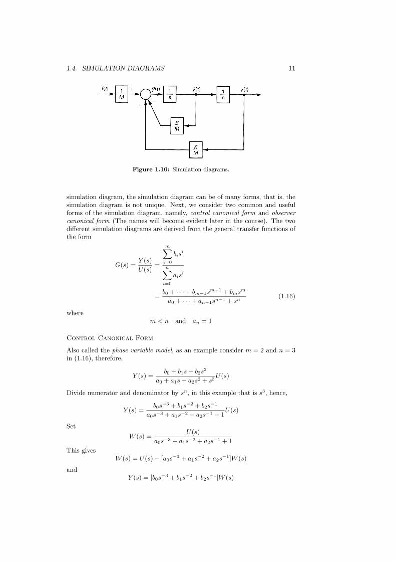
The input to the first integrator must be y(t). We can use these two integratorsto construct a simulation diagram of the mechanical system of Figure 1.1. Theinput to the cascaded integrators in Figure 1.9 is y(t) and the equation thaty(t) must satisfy for the mechanical system is obtained from (1.1) as
y(t) = − BMy(t)− K
My(t) +
1Mf(t)
Hence a summing junction and appropriate gains can be added to the blockdiagram of Figure 1.9 to satisfy this equation as shown in Figure 1.10.
1.4.1 State-variable models from Transfer Function
A simulation diagram constructed from the system differential equations willusually be unique. However, if the transfer function is used to construct the
1.4. SIMULATION DIAGRAMS 11
Figure 1.10: Simulation diagrams.
simulation diagram, the simulation diagram can be of many forms, that is, thesimulation diagram is not unique. Next, we consider two common and usefulforms of the simulation diagram, namely, control canonical form and observercanonical form (The names will become evident later in the course). The twodifferent simulation diagrams are derived from the general transfer functions ofthe form
G(s) =Y (s)U(s)
=
m∑i=0
bisi
n∑i=0
aisi
=b0 + · · ·+ bm−1s
m−1 + bmsm
a0 + · · ·+ an−1sn−1 + sn(1.16)
wherem < n and an = 1
Control Canonical Form
Also called the phase variable model, as an example consider m = 2 and n = 3in (1.16), therefore,
Y (s) =b0 + b1s+ b2s
2
a0 + a1s+ a2s2 + s3U(s)
Divide numerator and denominator by sn, in this example that is s3, hence,
Y (s) =b0s−3 + b1s
−2 + b2s−1
a0s−3 + a1s−2 + a2s−1 + 1U(s)
Set
W (s) =U(s)
a0s−3 + a1s−2 + a2s−1 + 1This gives
W (s) = U(s)− [a0s−3 + a1s
−2 + a2s−1]W (s)
andY (s) = [b0s−3 + b1s
−2 + b2s−1]W (s)
12 CHAPTER 1. LINEAR SYSTEMS
U(s) W (s)
Y (s)
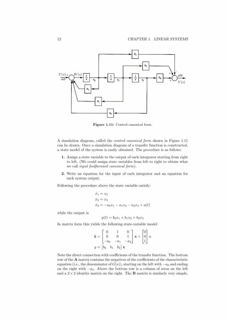
Figure 1.11: Control canonical form.
A simulation diagram, called the control canonical form shown in Figure 1.11can be drawn. Once a simulation diagram of a transfer function is constructed,a state model of the system is easily obtained. The procedure is as follows:
1. Assign a state variable to the output of each integrator starting from rightto left. (We could assign state variables from left to right to obtain whatwe call input feedforward canonical form).
2. Write an equation for the input of each integrator and an equation foreach system output.
Following the procedure above the state variable satisfy:
x1 = x2
x2 = x3
x3 = −a0x1 − a1x2 − a2x3 + u(t)
while the output isy(t) = b0x1 + b1x2 + b2x3
In matrix form this yields the following state-variable model
x =
0 1 00 0 1−a0 −a1 −a2
x +
001
uy =
[b0 b1 b2
]x
Note the direct connection with coefficients of the transfer function. The bottomrow of the A matrix contains the negatives of the coefficients of the characteristicequation (i.e., the denominator ofG(s)), starting on the left with−a0 and endingon the right with −a2. Above the bottom row is a column of zeros on the leftand a 2× 2 identity matrix on the right. The B matrix is similarly very simple,
1.4. SIMULATION DIAGRAMS 13
all the elements are zero except for the bottom element, which is the gain fromthe original system. The C matrix contains the positive of the coefficients of thenumerator of the transfer function, starting on the left with b0 and ending onthe right with b2. These equations are easily extended to the nth-order system.It is important to note that state matrices are never unique, and each G(s) hasinfinite number of state models.
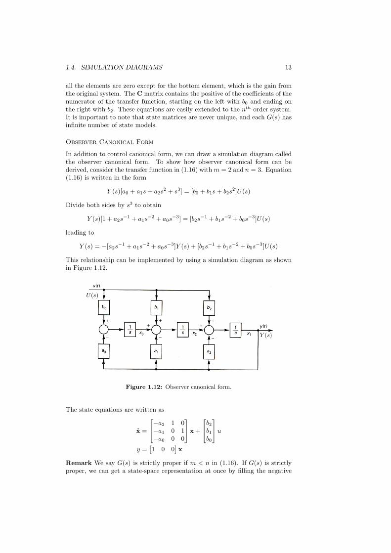
Observer Canonical Form
In addition to control canonical form, we can draw a simulation diagram calledthe observer canonical form. To show how observer canonical form can bederived, consider the transfer function in (1.16) with m = 2 and n = 3. Equation(1.16) is written in the form
Y (s)[a0 + a1s+ a2s2 + s3] = [b0 + b1s+ b2s
2]U(s)
Divide both sides by s3 to obtain
Y (s)[1 + a2s−1 + a1s
−2 + a0s−3] = [b2s−1 + b1s
−2 + b0s−3]U(s)
leading to
Y (s) = −[a2s−1 + a1s
−2 + a0s−3]Y (s) + [b2s−1 + b1s
−2 + b0s−3]U(s)
This relationship can be implemented by using a simulation diagram as shownin Figure 1.12.
U(s)
Y (s)
Figure 1.12: Observer canonical form.
The state equations are written as
x =
−a2 1 0−a1 0 1−a0 0 0
x +
b2b1b0
uy =
[1 0 0
]x
Remark We say G(s) is strictly proper if m < n in (1.16). If G(s) is strictlyproper, we can get a state-space representation at once by filling the negative
14 CHAPTER 1. LINEAR SYSTEMS
denominator coefficients into the lowermost row of A if a control canonical formis required and into the leftmost column if an observer canonical form is desired.If m = n, G(s) is proper, but not strictly proper. In this cases we have to dividethe numerator of G(s) by the denominator. This will lead to a feedthroughterm, i.e., the D matrix is not zero. If G(s) is not proper state-space represen-tations do not exist for non-proper transfer functions.
Find the state and output equations forExample 1.5
G(s) =5s2 + 7s+ 4
s3 + 3s2 + 6s+ 2
in control canonical form.
� Solution State equation
x =
0 1 00 0 1−2 −6 −3
x +
001
uThe output equation is
y =[4 7 5
]x �
Find the state and output equations forExample 1.6
G(s) =1
2s2 − s+ 3
� Solution State equation
x =[
0 1−3/2 1/2
]x +
[0
1/2
]u
The output equation isy =
[1 0
]x �
Write a state variable expression for the following differential equationExample 1.7
2y − y + 3y = u− 2u
� Solution If we attempt to use the definitions of state variables presentedearlier as in Example 1.4 we require derivatives of u in the state equations.According to the standard form of (1.14) and (1.15), this is not allowed. Weneed to eliminate the derivates of u. A useful formulation for state variableshere is to obtain a transfer function and then using a simulation diagram toobtain the state model. The transfer function of the system is
Y (s) =s− 2
2s2 − s+ 3U(s)
The state model in control canonical form is given by
x =[
0 1−3/2 1/2
]x +
[01
]u
y =[−1 1/2
]x
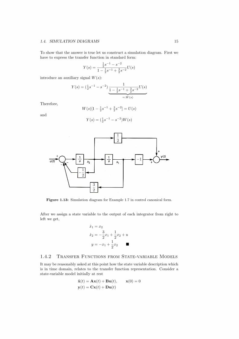
1.4. SIMULATION DIAGRAMS 15
To show that the answer is true let us construct a simulation diagram. First wehave to express the transfer function in standard form:
Y (s) =12s−1 − s−2
1− 12s−1 + 3
2s−2U(s)
introduce an auxiliary signal W (s):
Y (s) = ( 12s−1 − s−2)
11− 1
2s−1 + 3
2s−2U(s)︸ ︷︷ ︸
=:W (s)
Therefore,W (s)[1− 1
2s−1 + 3
2s−2] = U(s)
andY (s) = ( 1
2s−1 − s−2)W (s)
12
−1
−12
32
Figure 1.13: Simulation diagram for Example 1.7 in control canonical form.
After we assign a state variable to the output of each integrator from right toleft we get,
x1 = x2
x2 = −32x1 +
12x2 + u
y = −x1 +12x2 �
1.4.2 Transfer Functions from State-variable Models
It may be reasonably asked at this point how the state variable description whichis in time domain, relates to the transfer function representation. Consider astate-variable model initially at rest
x(t) = Ax(t) + Bu(t), x(0) = 0y(t) = Cx(t) + Du(t)
16 CHAPTER 1. LINEAR SYSTEMS
Taking Laplace transforms yields
sX(s) = AX(s) + BU(s)Y(s) = CX(s) + DU(s)
The term sX(s) must be written as sIX(s), where I is the identity matrix.This additional step is necessary, since the subtraction of the matrix A fromthe scalar s is not defined. Then,
sX(s)−AX(s) = (sI−A)X(s) = BU(s)
orX(s) = (sI−A)−1BU(s)
Substituting in the output equation, we get
Y(s) = C(sI−A)−1BU(s) + DU(s)
We conclude that the transfer function from U(s) to Y (s) is then
G(s) = C(sI−A)−1B + D
The state equations of a system are given byExample 1.8
x =[−2 0−3 −1
]x +
[12
]u
y =[3 1
]x
Determine the transfer function for the system.
� Solution The transfer function is given by
G(s) = C(sI−A)−1B + D
First, we calculate (sI−A)−1. Now,
sI−A = s
[1 00 1
]−[−2 0−3 −1
]=[s+ 2 0
3 s+ 1
]Therefore,
det(sI−A) = (s+ 2)(s+ 1) = s2 + 3s+ 2Then, letting det(sI−A) = ∆(s) for convenience, we have
(sI−A)−1 =adj(sI−A)det(sI−A)
=
s+ 1∆(s)
0
−3∆(s)
s+ 2∆(s)
and the transfer function is given by
G(s) =[3 1
] s+ 1∆(s)
0
−3∆(s)
s+ 2∆(s)
[12]
=[3 1
] s+ 1∆(s)
2s+ 1∆(s)
=5s+ 4
s2 + 3s+ 2�
1.5. SYSTEM INTERCONNECTIONS 17
1.5 System Interconnections
Frequently, a system is made up of components connected together in sometopology. This raises the question, if we have state models for components, howcan we assemble them into a state model for overall system?
1.5.1 Series and Parallel Connections
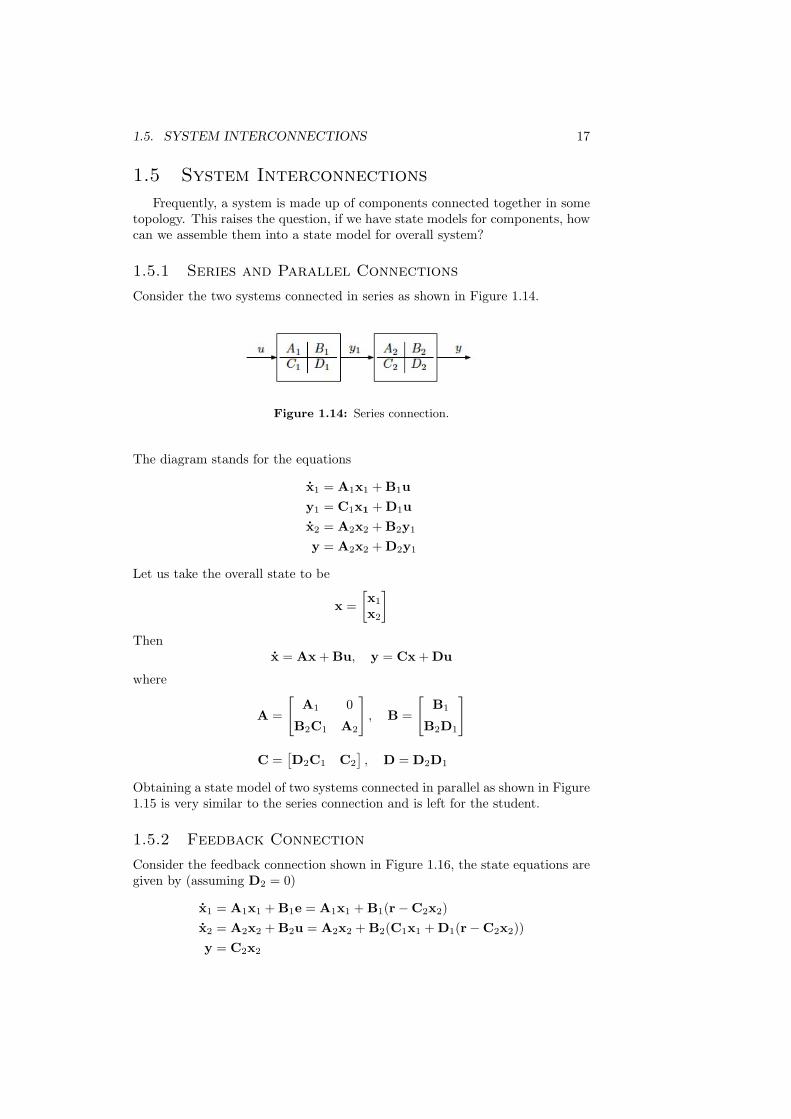
Consider the two systems connected in series as shown in Figure 1.14.
Figure 1.14: Series connection.
The diagram stands for the equations
x1 = A1x1 + B1u
y1 = C1x1 + D1u
x2 = A2x2 + B2y1
y = A2x2 + D2y1
Let us take the overall state to be
x =[x1
x2
]Then
x = Ax + Bu, y = Cx + Du
where
A =
[A1 0
B2C1 A2
], B =
[B1
B2D1
]
C =[D2C1 C2
], D = D2D1
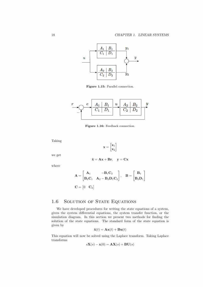
Obtaining a state model of two systems connected in parallel as shown in Figure1.15 is very similar to the series connection and is left for the student.
1.5.2 Feedback Connection
Consider the feedback connection shown in Figure 1.16, the state equations aregiven by (assuming D2 = 0)
x1 = A1x1 + B1e = A1x1 + B1(r−C2x2)x2 = A2x2 + B2u = A2x2 + B2(C1x1 + D1(r−C2x2))y = C2x2
18 CHAPTER 1. LINEAR SYSTEMS
Figure 1.15: Parallel connection.
Figure 1.16: Feedback connection.
Taking
x =[x1
x2
]we get
x = Ax + Br, y = Cx
where
A =
[A1 −B1C2
B2C1 A2 −B2D1C2
], B =
[B1
B2D1
]
C =[0 C2
]
1.6 Solution of State Equations
We have developed procedures for writing the state equations of a system,given the system differential equations, the system transfer function, or thesimulation diagram. In this section we present two methods for finding thesolution of the state equations. The standard form of the state equation isgiven by
x(t) = Ax(t) + Bu(t)
This equation will now be solved using the Laplace transform. Taking Laplacetransforms
sX(s)− x(0) = AX(s) + BU(s)
1.6. SOLUTION OF STATE EQUATIONS 19
We wish to solve this equation for X(s); to do this we reaarange the last equation
(sI−A)X(s) = x(0) + BU(s)
Pre-multiplying by (sI−A)−1, we obtain
X(s) = (sI−A)−1x(0) + (sI−A)−1BU(s) (1.17)
and the state vector x(t) is the inverse Laplace transform of this equation.Therefore,
x(t) = eAtx(0) +∫ t
0
eA(t−τ)Bu(τ) dτ (1.18)
if the initial time is t0, then
x(t) = eA(t−t0)x(0) +∫ t
t0
eA(t−τ)Bu(τ) dτ
The exponential matrix eAt is called the state transition matrix Φ(t) and isdefined as
Φ(t) = L−1(sI−A)−1 = eAt
andΦ(s) = (sI−A)−1
The exponential matrix eAt represents the following power series of the matrixAt, and
Φ(t) = eAt = I + At+12!
A2t2 +13!
A3t3 + · · · (1.19)
Equation (1.18) can be written as
x(t) = Φ(t)x(0) +∫ t
0
Φ(t− τ)Bu(τ) dτ (1.20)
In Equation (1.20) the first term represents the response to a set of initialconditions (zero-input response), whilst the integral term represents the reponseto a forcing function u(t) (zero-state response). Similarly, the output equationis given by
y(t) = CΦ(t)x(0) +∫ t
0
CΦ(t− τ)Bu(τ) dτ + Du(t) (1.21)
Use the infinite series in (1.19) to evaluate the transition matrix Φ(t) if Example 1.9
A =[0 10 0
]� Solution This is a good method only if A has a lot of zeros, since thisguarantees a quick convergence of the infinite series. Clearly,
A2 =[0 00 0
]
20 CHAPTER 1. LINEAR SYSTEMS
and we stop here, since A2 = 0 and any higher powers are zero. Therefore,
eAt = I + At =[1 t0 1
]�
The most common way of evaluating the transition matrix Φ(t) is with the useof Laplace, as the next Example demonstrates.
Use the Laplace transform to find the transition matrix if A is the same asExample 1.10in Example 1.9.
� Solution We first calculate the matrix (sI−A),
sI−A = s
[1 00 1
]−[0 10 0
]=[s −10 s
]The determinant of this matrix is
det(sI−A) = s2
and the adjoint matrix is
adj(sI−A) =[s 10 s
]Next we determine the inverse of the matrix (sI−A),
(sI−A)−1 =adj(sI−A)det(sI−A)
=1s2
[s 10 s
]
=
1s
1s2
01s
The state transition matrix is the inverse Laplace transform of this matrix
eAt = Φ(t) =[1 t0 1
]�
Consider the system described by the transfer functionExample 1.11
G(s) =1
s2 + 3s+ 2
(a) Write down the state equation in observer canonical form.
(b) Evaluate the state transition matrix Φ(t).
(c) Find the zero-state response if a unit step is applied.
� Solution (a) The state equation in observer canonical form is given by
x =[−3 1−2 0
]x +
[01
]u
1.6. SOLUTION OF STATE EQUATIONS 21
(b) To find the state transition matrix, we first calculate the matrix (sI−A),
sI−A = s
[1 00 1
]−[−3 1−2 0
]=[s+ 3 −1
2 s
]The determinant of this matrix is
det(sI−A) = s2 + 3s+ 2 = (s+ 1)(s+ 2)
and the adjoint matrix is
adj(sI−A) =[s 1−2 s+ 3
]Next we determine the inverse of the matrix (sI−A),
(sI−A)−1 =adj(sI−A)det(sI−A)
=
s
(s+ 1)(s+ 2)1
(s+ 1)(s+ 2)
−2(s+ 1)(s+ 2)
s+ 3(s+ 1)(s+ 2)
=
−1s+ 1
+2
s+ 21
s+ 1+−1s+ 2
−2s+ 1
+2
s+ 22
s+ 1+−1s+ 2
The state transition matrix is the inverse Laplace transform of this matrix
Φ(t) =[−e−t + 2e−2t e−t − e−2t
−2e−t + 2e−2t 2e−t − e−2t
](c) If a unit step is applied as an input. Then U(s) = 1/s, and the second termin (1.17) becomes
(sI−A)−1BU(s) =
s
(s+ 1)(s+ 2)1
(s+ 1)(s+ 2)
−2(s+ 1)(s+ 2)
s+ 3(s+ 1)(s+ 2)
[01]
1s
=
1
s(s+ 1)(s+ 2)
s+ 3s(s+ 1)(s+ 2)
=
12
s+−1s+ 1
+12
s+ 232
s+−2s+ 1
+12
s+ 2
The inverse Laplace transform of this term is
L−1((sI−A)−1BU(s)) =
12− e−t +
12e−2t
32− 2e−t +
12e−2t
22 CHAPTER 1. LINEAR SYSTEMS
Alternatively, we could have attempted a convolution solution,∫ t
0
Φ(t− τ)Bu(τ) dτ =∫ t
0
[−e−(t−τ) + 2e−2(t−τ) e−(t−τ) − e−2(t−τ)
−2e−(t−τ) + 2e−2(t−τ) 2e−(t−τ) − e−2(t−τ)
] [01
]dτ
=
∫ t
0
(e−(t−τ) − e−2(t−τ))dτ∫ t
0
(2e−(t−τ) − e−2(t−τ))dτ
=
(e−teτ − 1
2e−2te2τ
) ∣∣∣∣t0(
2e−teτ − 12e−2te2τ
) ∣∣∣∣t0
=
[(1− e−t)− 1
2 (1− e−2t)
2(1− e−t)− 12 (1− e−2t)
]
=
12− e−t +
12e−2t
32− 2e−t +
12e−2t
The result shows that the solution may be evaluated either by the Laplacetransform or the convolution integral. �
1.6.1 Properties of the State-Transition Matrix
Three properties of the state-transition matrix will now be derived.
1. Φ(0) = I. This result follows directly from (1.19) by setting t = 0. Thestate transition matrix from Example 1.11 is used to illustrate this prop-erty,
Φ(t) =[−e−t + 2e−2t e−t − e−2t
−2e−t + 2e−2t 2e−t − e−2t
](1.22)
Now,
Φ(0) =[−e0 + 2e0 e0 − e0−2e0 + 2e0 2e0 − e0
]=[1 00 1
]= I
2. Φ(t2− t1)Φ(t1− t0) = Φ(t2− t0). To prove this result, recall that Φ(t) =eAt, hence,
Φ(t2 − t1)Φ(t1 − t0) = eA(t2−t1)eA(t1−t0)
= eA(t2−t0) = Φ(t2 − t0)
To illustrate this property consider the following:
Φ(t2 − t1)Φ(t1 − t0) =[−e−(t2−t1) + 2e−2(t2−t1) e−(t2−t1) − e−2(t2−t1)
−2e−(t2−t1) + 2e−2(t2−t1) 2e−(t2−t1) − e−2(t2−t1)
]×[−e−(t1−t0) + 2e−2(t1−t0) e−(t1−t0) − e−2(t1−t0)
−2e−(t1−t0) + 2e−2(t1−t0) 2e−(t1−t0) − e−2(t1−t0)
]
1.6. SOLUTION OF STATE EQUATIONS 23
The (1,1) element of the product matrix is given by
(1,1) element = [−e−(t2−t1) + 2e−2(t2−t1)][−e−(t1−t0) + 2e−2(t1−t0)]
+ [e−(t2−t1) − e−2(t2−t1)][−2e−(t1−t0) + 2e−2(t1−t0)]
= [e−(t2−t0) − 2e−(t2+t1−2t0) − 2e−(2t2−t1−t0) + 4e−2(t2−t0)]
+ [−2e−(t2−t0) + 2e−(t2+t1−2t0) + 2e−(2t2−t1−t0) − 2e−2(t2−t0)]
Combining these terms yields
(1,1) element = −e−(t2−t0) + 2e−2(t2−t0)
which is the (1,1) element of Φ(t2 − t0). The other three elements of theproduct matrix can be verified in a like manner.
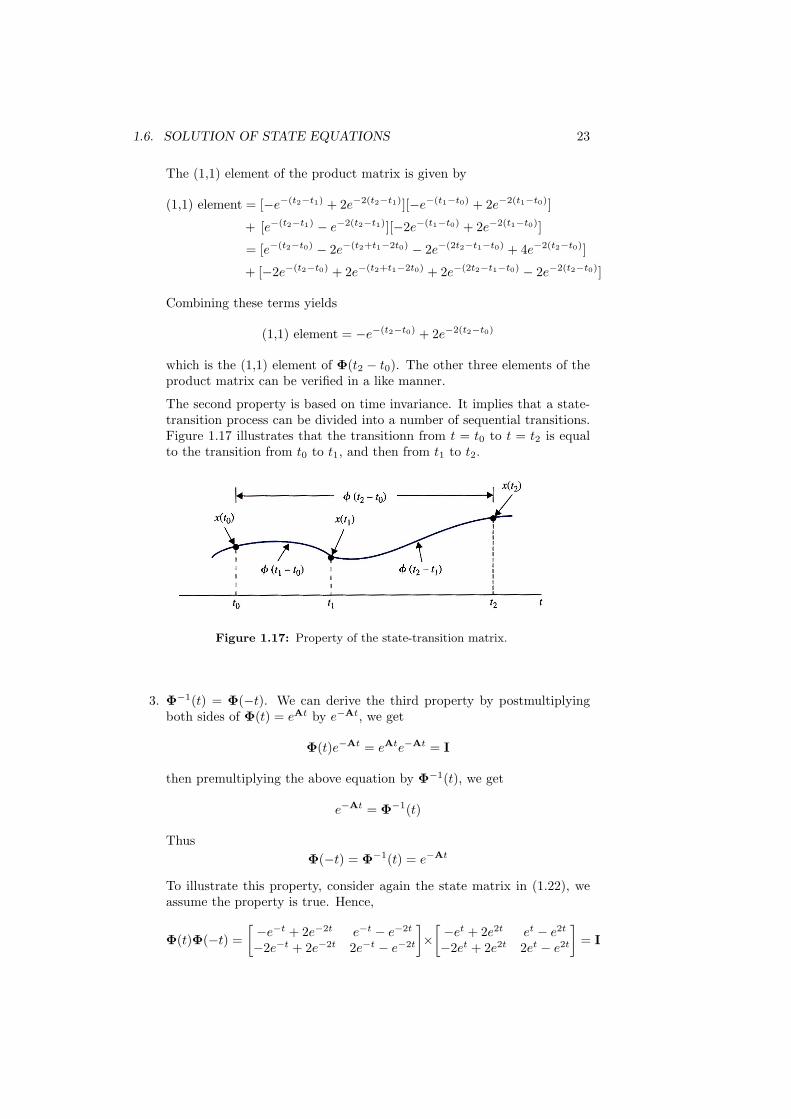
The second property is based on time invariance. It implies that a state-transition process can be divided into a number of sequential transitions.Figure 1.17 illustrates that the transitionn from t = t0 to t = t2 is equalto the transition from t0 to t1, and then from t1 to t2.
Figure 1.17: Property of the state-transition matrix.
3. Φ−1(t) = Φ(−t). We can derive the third property by postmultiplyingboth sides of Φ(t) = eAt by e−At, we get
Φ(t)e−At = eAte−At = I
then premultiplying the above equation by Φ−1(t), we get
e−At = Φ−1(t)
ThusΦ(−t) = Φ−1(t) = e−At
To illustrate this property, consider again the state matrix in (1.22), weassume the property is true. Hence,
Φ(t)Φ(−t) =[−e−t + 2e−2t e−t − e−2t
−2e−t + 2e−2t 2e−t − e−2t
]×[−et + 2e2t et − e2t−2et + 2e2t 2et − e2t
]= I
24 CHAPTER 1. LINEAR SYSTEMS
1.7 Characteristic Equations
Characteristic equations play an important role in the study of linear sys-tems. They can be defined with respect to differential equations, transfer func-tions, or state equations.
Characteristic Equation from a Differential Equation
Consider that a linear time-invariant system is described by the differentialequation
dny(t)dtn
+ an−1dn−1y(t)dtn−1
+ · · ·+ a1dy(t)dt
+ a0y(t)
= bmdmu(t)dtm
+ bm−1dm−1u(t)dtm−1
+ · · ·+ b1du(t)dt
+ b0u(t) (1.23)
where n > m. By defining the operator s as
sk =dk
dtkk = 1, 2, · · · , n
Equation (1.23) is written
(sn + an−1sn−1 + · · ·+ a1s+ a0)y(t) = (bmsm + bm−1s
m−1 + · · ·+ b1s+ b0)u(t)
The Characteristic equation of the the system is defined as
sn + an−1sn−1 + · · ·+ a1s+ a0 = 0 (1.24)
Characteristic Equation from a Transfer Function
The transfer function of the system described by (1.23) is
G(s) =bms
m + bm−1sm−1 + · · ·+ b1s+ b0
sn + an−1sn−1 + · · ·+ a1s+ a0
The characteristic equation is obtained by equating the denominator polynomialof the transfer function to zero.
Characteristic Equation from a State Equation
Recall thatG(s) = C(sI−A)−1B + D
which can be written as
G(s) = Cadj(sI−A)|sI−A|
B + D
=C[adj(sI−A)]B + |sI−A|D
|sI−A|
Setting the denominator of the transfer-function matrix G(s) to zero, we getthe characteristic equation
|sI−A| = 0
which is an alternative form of the characteristic equation, but should lead tothe same equation as in (1.24).
1.7. CHARACTERISTIC EQUATIONS 25
1.7.1 Eigenvalues
The roots of the characteristic equation are often referred to as the eigenvaluesof the matrix A.
Find the eigenvalues of the matrix A given by Example 1.12
A =[1 −10 −1
]
� Solution The characteristic equation of A is
|sI−A| = s2 − 1
Therefore, |sI−A| = 0 gives the eigenvalues λ1 = 1 and λ2 = −1. �
1.7.2 Eigenvectors
Any nonzero vector pi which satisfies the matrix equation
(λiI−A)pi = 0 (1.25)
where λi, i = 1, 2, · · · , n, denotes the ith eigenvalue of A, is called the eigen-vector of A associated with the eigenvalue λi. The procedure for determiningeigenvectors can be divided into two possible cases depending on the results ofthe eigenvalue calculations.
Case 1: All eigenvalues are distinct.
Case 2: Some eigenvalues are multiple roots of the characteristic equation.
Case 1: Distinct Eigenvalues
If A has distinct eigenvalues, the eigenvectors can be solved directly from (1.25).
Consider that a state equation has the matrix A given as in Example 1.12. Example 1.13Find the eigenvectors.
� Solution The eigenvalues were determined in Example 1.12 as λ1 = 1 andλ2 = −1. Let the eigenvectors be written as
p1 =[p11
p21
]p2 =
[p12
p22
]Substituting λ1 = 1 and p1 into (1.25), we get[
0 10 2
] [p11
p21
]=[00
]Thus, p21 = 0, and p11 is arbitrary which in this case can be set equal to 1.Similarly, for λ = −1, (1.25) becomes[
−2 10 0
] [p12
p22
]=[00
]
26 CHAPTER 1. LINEAR SYSTEMS
which leads to−2p12 + p22 = 0
The last equation has two unkowns, which means that one can be set arbitrarily.Let p12 = 1, then p22 = 2. The eigenvectors are
p1 =[10
]p2 =
[12
]�
Consider the matrixExample 1.14
A =[
1 3−6 −5
]� Solution The characteristic equation is s2 +4s+13. Thus A has eigenvalues−2±3j. We next find the eigenvectors associated with the eigenvalues. We firstfind [
λ− 1 −36 λ+ 5
]λ1=−2+3j
=[−3 + 3j −3
6 3 + 3j
]Then to find the related eigenvector we solve[
−3 + 3j −36 3 + 3j
] [p11
p21
]︸ ︷︷ ︸p1
=[00
]
which results in the two equations
−3p11(1− j)− 3p21 = 06p11 + 3p21(1 + j) = 0
orp21 = −p11(1− j)
Thus if we choose p11 = 1,
p1 =[
1−1 + j
]To find the other eigenvector we just conjugate the one already found, p1. Thus
p21 =[
1−1− j
]�
Case 2: Repeated Eigenvalues
An eigenvalue with multilpicity 2 or higher is called a repeated eigenvalue. IfA has repeated eigenvalues, not all eigenvectors can be found using (1.25). Weuse a variation of (1.25), called the generalized eigenvector. The next exampleillustrates the process of finding the eigenvectors.
Consider the matrixExample 1.15
A =[2 −82 −6
]� Solution The characteristic equation is s2 + 4s + 4. Thus, A has only one
1.8. SIMILARITY TRANSFORMATION 27
eigenvalue λ = −2 that is repeated twice. We first find the eigenvector forλ = −2 using (1.25). Therefore,[
λ− 2 8−2 λ+ 6
]λ=−2
[p11
p21
]︸ ︷︷ ︸p1
=[00
]
Making the substituition λ = −2 in the matrix yields[−4 8−2 4
] [p11
p21
]︸ ︷︷ ︸p1
=[00
]
resulting in the equations
−4p11 + 8p21 = 0−2p11 + 4p21 = 0
Both equations tell us the same thing, that
p11 = 2p21
Thus, one choice for the eigenvector is
p1 =[21
]For the generalized eigenvector that is associated with the second eigenvalue,we use a variation of the equation we used to find the eigenvector. That is, wewrite [
λ− 2 8−2 λ+ 6
]λ=−2
[p12
p22
]︸ ︷︷ ︸p2
= −[21
]
which yields the equations
−4p12 + 8p22 = −2−2p12 + 4p22 = −1
Either of these equations yields
p22 =2p12 − 1
4
Choosing p12 = 1/2 yields
p2 =
[12
0
]�
1.8 Similarity Transformation
In this chapter, procedures have been presented for finding a state-variablemodel from system differential equations, from system transfer functions, and
28 CHAPTER 1. LINEAR SYSTEMS
from system simulation diagrams. In this section, a procedure is given forfinding a different state model from a given state model. It will be shown thata system has an unlimited number of state models. However, while the internalcharacteristics are different, each state model for a system will have the sameinput-output characteristics (same transfer function).
The state model of an LTI single-input, single-output system is given by
x(t) = Ax(t) + Bu(t) (1.26)y(t) = Cx(t) +Du(t) (1.27)
where x(t) is the n × 1 state vector, u(t) and y(t) are the scalar input andoutput, respectively. Let us consider that the state model of Equations (1.26)and (1.27) and suppose that the state vector x(t) can be expressed as
x(t) = Pv(t) (1.28)
where P is an n × n nonsingular matrix, called a transformation matrix, orsimply, a transformation. We can write,
v(t) = P−1x(t)
Substituting (1.28) into the state equation in (1.26) yields
Pv(t) = APv(t) + Bu(t)
Premultiplying the above equation by P−1 to solve for v(t) results in the statemodel for the state vector v(t):
v(t) = P−1APv(t) + P−1Bu(t) (1.29)
Using (1.28), we find that the output equation in (1.27) becomes
y(t) = CPv(t) +Du(t) (1.30)
We have the state equations expressed as a function of the state vector x(t) in(1.26) and (1.27) and as a function of the transformed state vector v(t) in (1.29)and (1.30).
The state equations as a function of v(t) can be expressed in the standardformat as
v(t) = Avv(t) + Bvu(t) (1.31)
andy(t) = Cvx(t) +Dvu(t) (1.32)
Comparing (1.29) with (1.31) we get
Av = P−1AP
andBv = P−1B
Similarly, comparing (1.30) with (1.32), we see that
Cv = CP
andDv = D
The transformation just described is called a similarity transformation, since inthe transformed system such properties as the characteristic equation, eigenvec-tors, eigenvalues, and transfer functions are all preserved by the transformation.
1.8. SIMILARITY TRANSFORMATION 29
1.8.1 Properties of the Similarity Transformation
1. The eigenvalues of A and Av are equal. Consider the determinant of(sI−Av),
|sI−Av| = |sI−P−1AP| = |sP−1IP−P−1AP|= |P−1(sI−A)P|
Since the determinant of a product matrix is equal to the product of thedeterminants of the matrices, the last equation becomes
|sI−Av| = |P−1||sI−A||P| = |sI−A|
Thus the characteristic equation is preserved, which naturally leads to thesame eigenvalues.
2. The following transfer functions are equal:
Cv(sI−Av)−1Bv +Dv = C(sI−A)−1B +D
This can be easily seen since,
Gv(s) = Cv(sI−Av)−1Bv +Dv
= CP(sI−P−1AP)−1P−1B +D
which is simplified to
Gv(s) = C(sI−A)−1B +D = G(s)
Next we show how to choose the transformation matrix P to obtain a partic-ular form. When carrying out analysis and design in the state space representa-tion, it is often advantageous to transform these equations into particular forms.We shall describe the diagonal canonical form, the control canonical form, andthe observer canonical form. The transformation equations are given withoutproofs.
1.8.2 Diagonal Canonical Form
This form makes use of the eigenvectors. If A has distinct eigenvalues, there isa nonsingular transformation P that can be formed by use of the eigenvectorsof A as its columns; that is
P =[p1 p2 p3 · · · pn
]where pi, i = 1, 2, · · · , n, denotes the eigenvector associated with the eigenvalueλi. The Av matrix is a diagonal matrix,
Av =
λ1 0 0 · · · 00 λ2 0 · · · 00 0 λ3 · · · 0...
......
. . ....
0 0 0 · · · λn
30 CHAPTER 1. LINEAR SYSTEMS
where λ1, λ2, · · · , λn are the n distinct eigenvalues of A.
Consider the matrixExample 1.16
A =[1 −10 −1
]which has eigenvalues λ1 = 1 and λ2 = −1. The eigenvectors where determinedin example 1.13 to be
p1 =[10
]p2 =
[12
]Thus,
P =[p1 p2
]=[1 10 2
]and the diagonal canonical form of A is written
Av = P−1AP =12
[2 −10 1
] [1 −10 −1
] [1 10 2
]=[1 00 −1
]�
In general, when the matrix A has repeated eigenvalues, it cannot be trans-formed into a diagonal matrix. However, there exists a similarity transforma-tion such that the Av matrix is almost diagonal. the matrix Av is called theJordan canonical form. A typical Jordan canonical form is shown below
A =
λ1 1 0 0 00 λ1 1 0 00 0 λ1 0 00 0 0 λ2 00 0 0 0 λ3
where it is assumed that A has a repeated eigenvalue λ1 and distinct eigenvaluesλ2 and λ3. The Jordan canonical form generally has the following properties:
1. The elements on the main diagonal are the eigenvalues.
2. All elements below the main diagonal are zero.
3. Some of the elements immediately above the repeated eigenvalues on themain diagonal are 1s.
Consider the matrixExample 1.17
A =[2 −82 −6
]A has only one eigenvalue λ = −2 that is repeated twice. The generalizedeigenvector were found in example 1.15 to be
p1 =[21
]p2 =
[12
0
]Thus,
P =[p1 p2
]=
[2 1
2
1 0
]
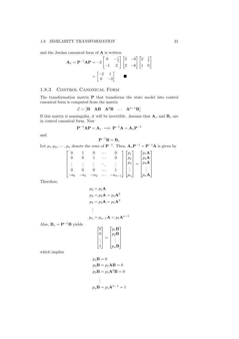
1.8. SIMILARITY TRANSFORMATION 31
and the Jordan canonical form of A is written
Av = P−1AP = −2
[0 − 1
2
−1 2
][2 −8
2 −6
][2 1
2
1 0
]
=[−2 10 −2
]�
1.8.3 Control Canonical Form
The transformation matrix P that transforms the state model into controlcanonical form is computed from the matrix
C =[B AB A2B · · · An−1B
]If this matrix is nonsingular, it will be invertible. Assume that Av and Bv arein control canonical form. Now
P−1AP = Av =⇒ P−1A = AvP−1
andP−1B = Bv
Let p1, p2, · · · , pn denote the rows of P−1. Then, AvP−1 = P−1A is given by0 1 0 · · · 00 0 1 · · · 0...
......
. . ....
0 0 0 · · · 1−a0 −a1 −a2 · · · −an−1
p1
p2
p3
...pn
=
p1Ap2Ap3A
...pnA
Therefore,
p2 = p1A
p3 = p2A = p1A2
p4 = p3A = p1A3
...
pn = pn−1A = p1An−1
Also, Bv = P−1B yields 00...1
=
p1Bp2B
...pnB
which implies
p1B = 0p2B = p1AB = 0
p3B = p1A2B = 0...
pnB = p1An−1 = 1
32 CHAPTER 1. LINEAR SYSTEMS
therefore, in vector matrix form, we have
p1
[B AB A2B · · · An−1B
]︸ ︷︷ ︸=C
=[0 0 0 · · · 1
]Hence,
p1 =[0 0 0 · · · 1
]C−1
Having found p1 we can now go back and construct all the rows of P−1. Notethat we are only interested in the last row of C−1 to define p1.
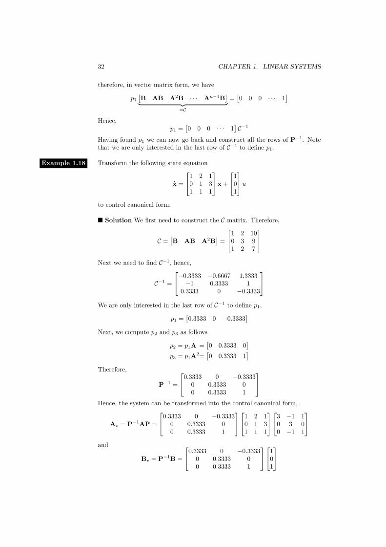
Transform the following state equationExample 1.18
x =
1 2 10 1 31 1 1
x +
101
uto control canonical form.
� Solution We first need to construct the C matrix. Therefore,
C =[B AB A2B
]=
1 2 100 3 91 2 7
Next we need to find C−1, hence,
C−1 =
−0.3333 −0.6667 1.3333−1 0.3333 1
0.3333 0 −0.3333
We are only interested in the last row of C−1 to define p1,
p1 =[0.3333 0 −0.3333
]Next, we compute p2 and p3 as follows
p2 = p1A =[0 0.3333 0
]p3 = p1A2=
[0 0.3333 1
]Therefore,
P−1 =
0.3333 0 −0.33330 0.3333 00 0.3333 1
Hence, the system can be transformed into the control canonical form,
Av = P−1AP =
0.3333 0 −0.33330 0.3333 00 0.3333 1
1 2 10 1 31 1 1
3 −1 10 3 00 −1 1
and
Bv = P−1B =
0.3333 0 −0.33330 0.3333 00 0.3333 1
101
1.8. SIMILARITY TRANSFORMATION 33
Thus, the control canonical form model is given by
v =
0 1 00 0 13 1 3
v +
001
uwhich could have been determined once the coefficients of the characteristicequation are known; however the exercise is to show how the control canonicaltransformation matrix P is obtained.
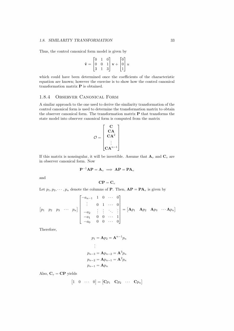
1.8.4 Observer Canonical Form
A similar approach to the one used to derive the similarity transformation of thecontrol canonical form is used to determine the transformation matrix to obtainthe observer canonical form. The transformation matrix P that transforms thestate model into observer canonical form is computed from the matrix
O =
C
CACA2
...CAn−1
If this matrix is nonsingular, it will be invertible. Assume that Av and Cv arein observer canonical form. Now
P−1AP = Av =⇒ AP = PAv
andCP = Cv
Let p1, p2, · · · , pn denote the columns of P. Then, AP = PAv is given by
[p1 p2 p3 · · · pn
]
−an−1 1 0 · · · 0... 0 1 · · · 0
−a2
......
. . ....
−a1 0 0 · · · 1−a0 0 0 · · · 0
=[Ap1 Ap2 Ap3 · · ·Apn
]
Therefore,
p1 = Ap2 = An−1pn
...
pn−3 = Apn−2 = A3pn
pn−2 = Apn−1 = A2pn
pn−1 = Apn
Also, Cv = CP yields[1 0 · · · 0
]=[Cp1 Cp2 · · · Cpn
]
34 CHAPTER 1. LINEAR SYSTEMS
which implies
Cp1 = CAn−1pn = 1...
Cpn−2 = CA2pn = 0Cpn−1 = CApn = 0
Cpn = 0
therefore, in vector matrix form, we haveC
CACA2
...CAn−1
︸ ︷︷ ︸
=O
pn =
000...1
Hence,
pn = O−1
000...1
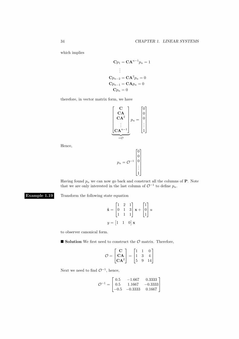
Having found pn we can now go back and construct all the columns of P. Notethat we are only interested in the last column of O−1 to define pn.
Transform the following state equationExample 1.19
x =
1 2 10 1 31 1 1
x +
101
uy =
[1 1 0
]x
to observer canonical form.
� Solution We first need to construct the O matrix. Therefore,
O =
CCACA2
=
1 1 01 3 45 9 14
Next we need to find O−1, hence,
O−1 =
0.5 −1.667 0.33330.5 1.1667 −0.3333−0.5 −0.3333 0.1667
1.8. SIMILARITY TRANSFORMATION 35
We are only interested in the last column of O−1 to define p3, in this case
p3 =
0.3333−0.33330.1667
Next, we compute p1 and p2 as follows
p1 = A2p3 =
0.33330.66670.1667
p2 = Ap3 =
−0.16670.16670.1667
Therefore,
P =
0.3333 −0.1667 0.33330.6667 0.1667 −0.33330.1667 0.1667 0.1667
Hence, the system can be transformed into the observer canonical form,
Av = P−1AP =
1 1 0−2 0 41 −1 2
1 2 10 1 31 1 1
0.3333 −0.1667 0.33330.6667 0.1667 −0.33330.1667 0.1667 0.1667
and
Cv = CP =[1 1 0
] 0.3333 −0.1667 0.33330.6667 0.1667 −0.33330.1667 0.1667 0.1667
Thus, the observer canonical form model is given by
x =
3 1 01 0 13 0 0
v +
123
uy =
[1 0 0
]x
which could have been determined once the coefficients of the characteristicequation are known; however the exercise is to show how the observer canonicaltransformation matrix P is obtained.

36 CHAPTER 1. LINEAR SYSTEMS
Chapter 2Controllability and Observability
Controllability and observability represent two major concepts of modern con-trol system theory. These concepts were originally introduced by R. Kalman in1960, and are particularly important for practical implementations. They canbe roughly defined as follows:
Controllability: In order to be able to do whatever we want with the givendynamic system under control input, the system must be controllable.
Observability: In order to see what is going on inside the system underobservation, the system must be observable.
In this chapter we will investigate the controllability and observability prop-erties of linear systems. We will see later in the course that the first stage ofthe design of a linear controller is often the investigation of controllability andobservability.
2.1 Motivation Examples
It is often a common practice in control applications to design a control in-put u(t) that makes the output y(t) behave in a desired manner. If one focuseson input/output behavior without thinking about system states, problems maybe encountered. That is to say, if we restrict our attention to designing inputsthat make the output behave in a desirable way, problems may rise. If one hasa state space model, then it is possible that while you are making the outputsbehave nicely, some of the states x(t) may be misbehaving badly. This is bestillustrated with the following examples.
Consider the system Example 2.1
x =[0 11 0
]x +
[01
]u
y =[1 −1
]x
We compute the transition matrix
Φ(t) =
[12 (et + e−t) 1
2 (et − e−t)12 (et − e−t) 1
2 (et + e−t)
]
37
38 CHAPTER 2. CONTROLLABILITY AND OBSERVABILITY
and so, if we use the initial condition x(0) = 0, and the input u(t) is the unitstep function we get
x(t) =∫ t
0
[12
(e(t−τ) + e−(t−τ)) 1
2
(e(t−τ) − e−(t−τ))
12
(e(t−τ) − e−(t−τ)) 1
2
(e(t−τ) + e−(t−τ))
] [0
1
]dτ
=
[12 (et + e−t)− 112 (et + e−t)
]
The output is
y(t) = e−t − 1
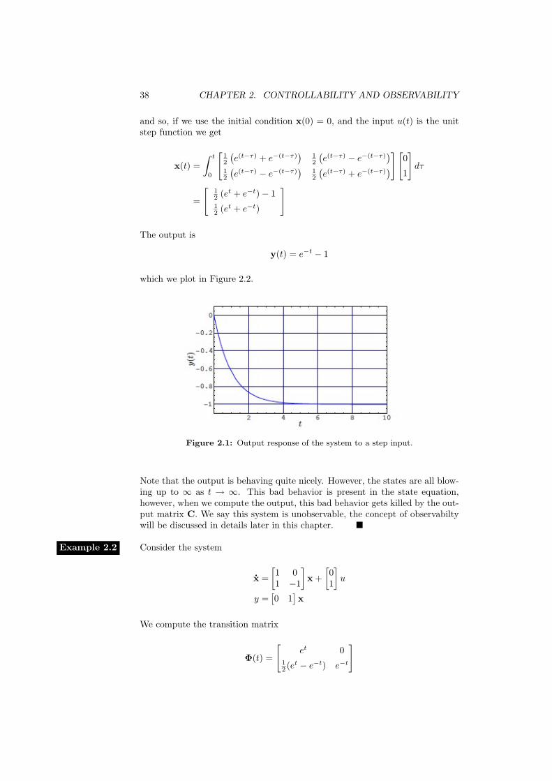
which we plot in Figure 2.2.
Figure 2.1: Output response of the system to a step input.
Note that the output is behaving quite nicely. However, the states are all blow-ing up to ∞ as t → ∞. This bad behavior is present in the state equation,however, when we compute the output, this bad behavior gets killed by the out-put matrix C. We say this system is unobservable, the concept of observabiltywill be discussed in details later in this chapter. �
Consider the systemExample 2.2
x =[1 01 −1
]x +
[01
]u
y =[0 1
]x
We compute the transition matrix
Φ(t) =
[et 0
12 (et − e−t) e−t
]
2.2. CONTROLLABILITY 39
and so, if we use the initial condition x(0) = 0, and the input u(t) is the unitstep function we get
x(t) =∫ t
0
[e(t−τ) 0
12
(e(t−τ) − e−(t−τ)) e−(t−τ)
][0
1
]dτ
=
[0
1− e−t
]
The output isy(t) = 1− e−t
Everything looks okay, the output is behaving nicely, and the states are notblowing up to ∞. Let’s change the initial condition to x(0) = (1, 0). We thencompute
x(t) =
[et
1 + 12 (et − 3e−t)
]and
y(t) = 1 +12
(et − 3e−t)
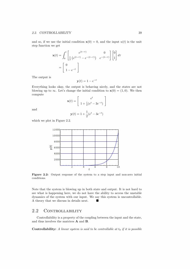
which we plot in Figure 2.2.
Figure 2.2: Output response of the system to a step input and non-zero initialconditions.
Note that the system is blowing up in both state and output. It is not hard tosee what is happening here, we do not have the ability to access the unstabledynamics of the system with our input. We say this system is uncontrollable.A theory that we discuss in details next. �
2.2 Controllability
Controllability is a property of the coupling between the input and the state,and thus involves the matrices A and B.
Controllability: A linear system is said to be controllable at t0 if it is possible
40 CHAPTER 2. CONTROLLABILITY AND OBSERVABILITY
to find some input function u(t), that when applied to the system will transferthe initial state x(t0) to the origin at some finite time t1, i.e., x(t1) = 0.
Some authors define another kind of controllability involving the output y(t).The definition given above is referred to as state controllability. It is the mostcommon definition, and is the only type used in this course, so the adjective”state” is omitted. If a system is not completely controllable, then for someinitial states no input exists which can drive the system to the zero state. Atrivial example of an uncontrollable system arises when the matrix B is zero,because then the input is disconnected from the state.
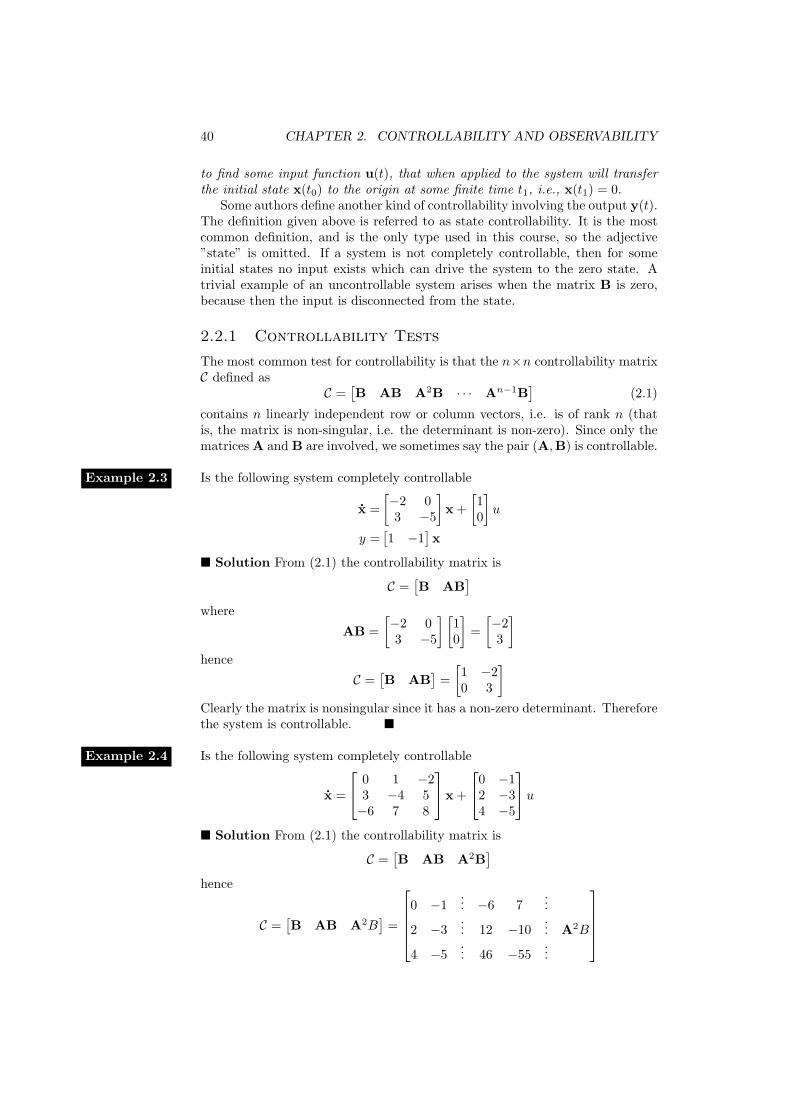
2.2.1 Controllability Tests
The most common test for controllability is that the n×n controllability matrixC defined as
C =[B AB A2B · · · An−1B
](2.1)
contains n linearly independent row or column vectors, i.e. is of rank n (thatis, the matrix is non-singular, i.e. the determinant is non-zero). Since only thematrices A and B are involved, we sometimes say the pair (A,B) is controllable.
Is the following system completely controllableExample 2.3
x =[−2 03 −5
]x +
[10
]u
y =[1 −1
]x
� Solution From (2.1) the controllability matrix is
C =[B AB
]where
AB =[−2 03 −5
] [10
]=[−23
]hence
C =[B AB
]=[1 −20 3
]Clearly the matrix is nonsingular since it has a non-zero determinant. Thereforethe system is controllable. �
Is the following system completely controllableExample 2.4
x =
0 1 −23 −4 5−6 7 8
x +
0 −12 −34 −5
u� Solution From (2.1) the controllability matrix is
C =[B AB A2B
]hence
C =[B AB A2B
]=
0 −1
... −6 7...
2 −3... 12 −10
... A2B
4 −5... 46 −55
...
2.3. OBSERVABILITY 41
Since the first three columns are linearly independent we can conclude thatrank C = 3. Hence there is no need to compute A2B since it is well knownfrom linear algebra that the row rank of the given matrix is equal to its columnrank. Thus, rank C = 3 = n implies that the system under considerationis controllable. Alternatively since C is nonsquare, we could have formed thematrix CC′
, which is n× n; then if CC′is nonsingular, C has rank n. �
There are several alternate methods for testing controllability, and some ofthese may be more convenient to apply than the condition in (2.1).
Control Canonical Form
The pair (A,B) is completely controllable if A and B are in control canonicalform or transformable into control canonical form by a similarity transformation.
Diagonal Canonical Form
If A is diagonal and has distinct eigenvalues. Then, the pair (A,B) is control-lable if B does not have any row with all zeros.
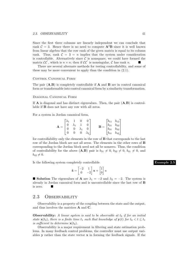
For a system in Jordan canonical form,
A =
λ1 1 0 00 λ1 1 00 0 λ1 00 0 0 λ2
B =
b11 b12b21 b22b31 b32b41 b42
for controllability only the elements in the row of B that corresponds to the lastrow of the Jordan block are not all zeros. The elements in the other rows of Bcorresponding to the Jordan block need not all be nonzero. Thus, the conditionof controllability for the above (A,B) pair is b31 6= 0, b32 6= 0, b41 6= 0, andb42 6= 0.
Is the following system completely controllable Example 2.5
x =[−2 10 −2
]x +
[10
]u
� Solution The eigenvalues of A are λ1 = −2 and λ2 = −2. The system isalready in Jordan canonical form and is uncontrollable since the last row of Bis zero. �
2.3 Observability
Observability is a property of the coupling between the state and the output,and thus involves the matrices A and C.
Observability: A linear system is said to be observable at t0 if for an initialstate x(t0), there is a finite time t1 such that knowledge of y(t) for t0 < t ≤ t1is sufficient to determine x(t0).
Observability is a major requirement in filtering and state estimation prob-lems. In many feedback control problems, the controller must use output vari-ables y rather than the state vector x in forming the feedback signals. If the
42 CHAPTER 2. CONTROLLABILITY AND OBSERVABILITY
system is observable, then y contains sufficient information about the internalstates.
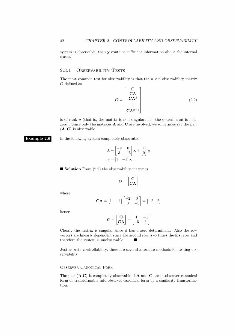
2.3.1 Observability Tests
The most common test for observability is that the n× n observability matrixO defined as
O =
C
CACA2
...CAn−1
(2.2)
is of rank n (that is, the matrix is non-singular, i.e. the determinant is non-zero). Since only the matrices A and C are involved, we sometimes say the pair(A,C) is observable.
Is the following system completely observableExample 2.6
x =[−2 03 −5
]x +
[10
]u
y =[1 −1
]x
� Solution From (2.2) the observability matrix is
O =[
CCA
]where
CA =[1 −1
] [−2 03 −5
]=[−5 5
]hence
O =[
CCA
]=[
1 −1−5 5
]Clearly the matrix is singular since it has a zero determinant. Also the rowvectors are linearly dependent since the second row is -5 times the first row andtherefore the system is unobservable. �
Just as with controllability, there are several alternate methods for testing ob-servability.
Observer Canonical Form
The pair (A,C) is completely observable if A and C are in observer canonicalform or transformable into observer canonical form by a similarity transforma-tion.
2.4. FREQUENCY DOMAIN TESTS 43
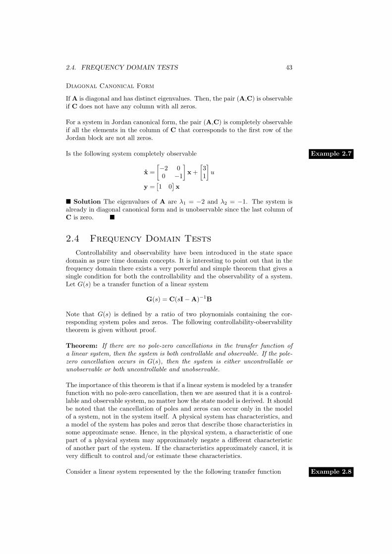
Diagonal Canonical Form
If A is diagonal and has distinct eigenvalues. Then, the pair (A,C) is observableif C does not have any column with all zeros.
For a system in Jordan canonical form, the pair (A,C) is completely observableif all the elements in the column of C that corresponds to the first row of theJordan block are not all zeros.
Is the following system completely observable Example 2.7
x =[−2 00 −1
]x +
[31
]u
y =[1 0
]x
� Solution The eigenvalues of A are λ1 = −2 and λ2 = −1. The system isalready in diagonal canonical form and is unobservable since the last column ofC is zero. �
2.4 Frequency Domain Tests
Controllability and observability have been introduced in the state spacedomain as pure time domain concepts. It is interesting to point out that in thefrequency domain there exists a very powerful and simple theorem that gives asingle condition for both the controllability and the observability of a system.Let G(s) be a transfer function of a linear system
G(s) = C(sI−A)−1B
Note that G(s) is defined by a ratio of two ploynomials containing the cor-responding system poles and zeros. The following controllability-observabilitytheorem is given without proof.
Theorem: If there are no pole-zero cancellations in the transfer function ofa linear system, then the system is both controllable and observable. If the pole-zero cancellation occurs in G(s), then the system is either uncontrollable orunobservable or both uncontrollable and unobservable.
The importance of this theorem is that if a linear system is modeled by a transferfunction with no pole-zero cancellation, then we are assured that it is a control-lable and observable system, no matter how the state model is derived. It shouldbe noted that the cancellation of poles and zeros can occur only in the modelof a system, not in the system itself. A physical system has characteristics, anda model of the system has poles and zeros that describe those characteristics insome approximate sense. Hence, in the physical system, a characteristic of onepart of a physical system may approximately negate a different characteristicof another part of the system. If the characteristics approximately cancel, it isvery difficult to control and/or estimate these characteristics.
Consider a linear system represented by the the following transfer function Example 2.8
44 CHAPTER 2. CONTROLLABILITY AND OBSERVABILITY
G(s) =(s+ 3)
(s+ 1)(s+ 2)(s+ 3)=
s+ 3s3 + 6s2 + 11s+ 6
The above theorem indicates that any state model for this system is eitheruncontrollable or/and unobservable. To get the complete answer we have to goto a state space form and examine the controllability and observability matrices.One of the many possible state models of G(s) is as follows
x =
0 1 00 0 1−6 −11 −6
x +
001
uy =
[3 1 0
]x
It is easy to show that the controllability and observability matrices are givenby
C =
0 0 10 1 −61 −6 25
O =
3 1 00 3 1−6 −11 −3
Since
det C = 1 6= 0 =⇒ rank C = 3 = n
anddet O = 0 6= 0 =⇒ rank O < 3 = n
this system is controllable, but unobservable. �
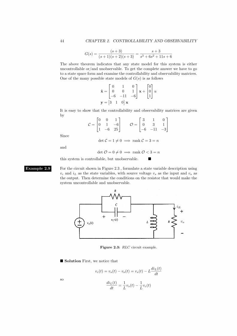
For the circuit shown in Figure 2.3 , formulate a state variable description usingExample 2.9vc and iL as the state variables, with source voltage vs as the input and vo asthe output. Then determine the conditions on the resistor that would make thesystem uncontrollable and unobservable.
iR
vo
Figure 2.3: RLC circuit example.
� Solution First, we notice that
vc(t) = vs(t)− vo(t) = vs(t)− LdiL(t)dt
sodiL(t)dt
=1Lvs(t)−
1Lvc(t)
2.4. FREQUENCY DOMAIN TESTS 45
which is one of the necessary state equations. Furthermore, for the capacitorvoltage,
dvc(t)dt
=1Cic(t)
=1C
(iL(t) + iR(t)− vc(t)
R
)=
1C
(iL(t) +
vs(t)− vc(t)R
− vc(t)R
)=iL(t)C− 2vc(t)
RC+vs(t)RC
Therefore, the state equations are:[vc(t)
iL(t)
]=
[− 2RC
1C
− 1L 0
][vc(t)
iL(t)
]+
[1RC
1L
]vs(t)
vx(t) =[−1 0
] [vc(t)iL(t)
]+ vs(t)
Testing controllability
C =[B AB
]=
1RC
− 2R2C2
+1LC
1L
− 1RLC
The nonsingularity of this matrix can be checked by determining the determi-nant ∣∣∣∣∣∣∣
1RC
− 2R2C2
+1LC
1L
− 1RLC
∣∣∣∣∣∣∣ =1
R2LC2− 1L2C
Clearly the condition under which the determinant is zero is
R =
√L
C
Similarly, the observability matrix is:
O =
−1 02RC
− 1C
which obviously is always nonsingular. Hence, the system is always observable,
but becomes uncontrollable whenever R =√
LC .
If we were to calculate the transfer function between the output vx(t) andthe input vs(t), (using basic circuit analysis), we obtain the following transferfunction:
vxvs
=s
(s+
1RC
)s2 +
2RC
s+1LC
46 CHAPTER 2. CONTROLLABILITY AND OBSERVABILITY
If R =√
LC then the roots of the characteristic equation are given by
s1,2 = − 1RC
giving a system with repeated roots at s = − 1RC . Thus, in pole-zero form, we
have
vxvs
=s
(s+
1RC
)(s+
1RC
)(s+
1RC
) =s(
s+1RC
)which is now a first order system. The energy storage elements, in conjunctionwith this particular resistance value, are interacting in such a way that theireffects combine, giving an equivalent first-order system. In this case, the timeconstants due to these two elements are the same, making them equivalent to asingle element. �
2.5 Similarity Transformations Again
In this section we investigate the effects of the similarity transformations oncontrollability and observability. Consider a linear system with controllabilitymatrix
C =[B AB · · · An−1B
]Under a similarity transformation, we will have transformed matrices
Av = P−1AP Bv = P−1B
Therefore, in this new basis, the controllability test will give
Cv =[Bv AvBv A2
vBv · · ·]
=[P−1B P−1APP−1B P−1APP−1APP−1B · · ·
]=[P−1B P−1AB P−1A2B · · ·
]=[P−1B P−1AB · · · P−1An−1B
]= P−1
[B AB · · · An−1B
]= P−1C
Because P is nonsingular, rank Cv = rank C. An analogous process shows thatrankOv = rankO. Thus, a system that is controllable (observable) will remainso after the application of a similarity transformation.
Chapter 3Stability
Stability is the most crucial issue in designing any control system. One of themost common control problems is the design of a closed loop system such thatits output follows its input as closely as possible. If the system is unstable suchbehavior is not guaranteed. Unstable systems have at least one of the statevariables blowing up to infinity as time increases. This usually cause the systemto suffer serious damage such as burn out, break down or it may even explode.Therefore, for such reasons our primary goal is to guarantee stability. As soonas stability is achieved one seeks to satisfy other design requirements, such asspeed of response, settling time, steady state error, etc.
3.1 Introduction
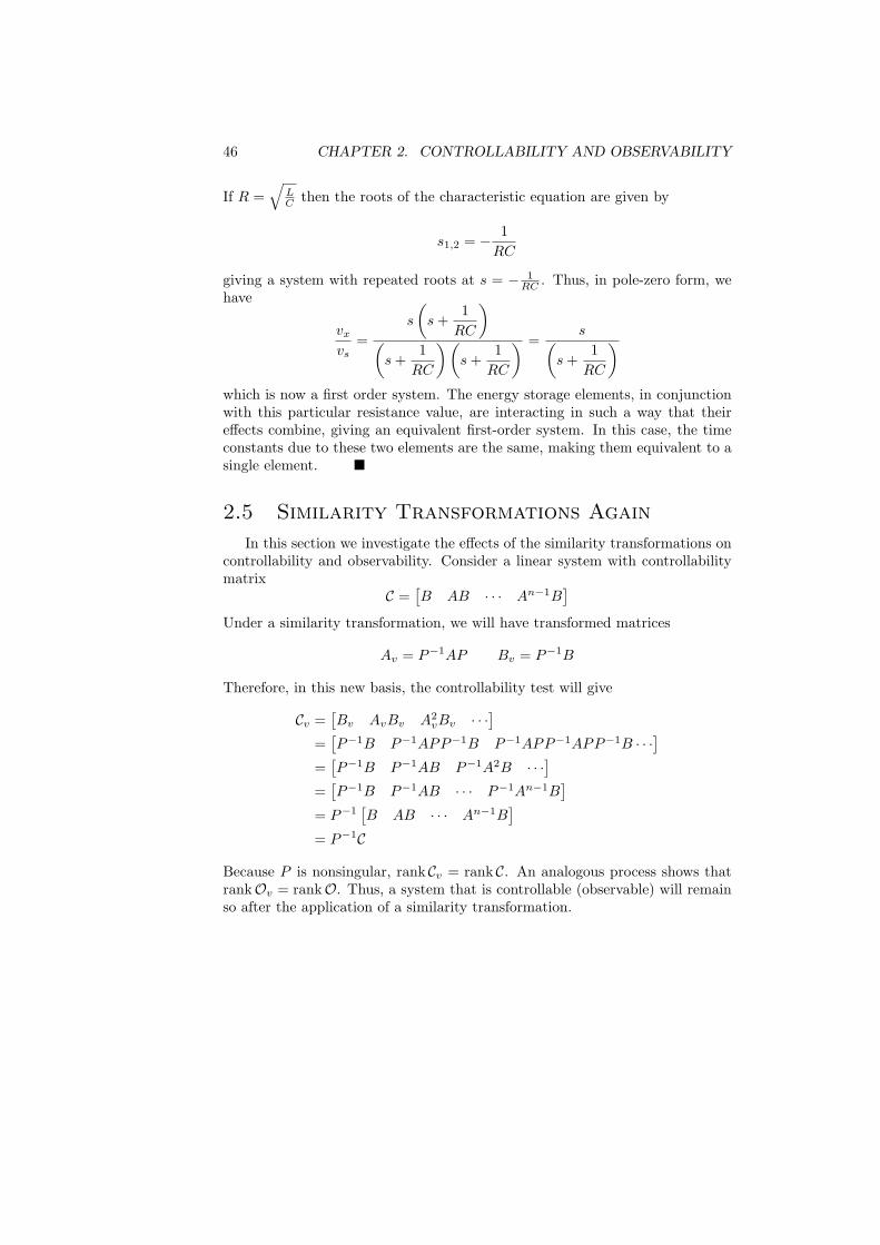
To help make the later mathematical treatment of stability more intuitive letus begin with a general discussion of stability concepts and equilibrium points.Consider the ball which is free to roll on the surface shown in Figure 3.1. Theball could be made to rest at points A, E, F , and G and anywhere betweenpoints B and D, such as at C. Each of these points is an equilibrium point ofthe system.
In state space, an equilibrium point for a sytem is a point at which x is zeroin the absence of all inputs and disruptive disturbances. Thus if the system isplaced in that state, it will remain there.
Figure 3.1: Equilibrium points
47
48 CHAPTER 3. STABILITY
A small perturbation away from points A or F will cause the ball to divergefrom these points. This behavior justifies labeling points A and F as unstableequilibrium points. After small perturbations away from E and G, the ball willeventually return to rest at these points. Thus E and G are labeled as stableequilibrium points. If the ball is displaced slightly from point C, it will normallystay at the new position. Points like C are sometimes said to be neutrally stable.
So far we assumed small perturbations, if the ball was displaced sufficientlyfar from point G, it would not return to that point. We say the system is stablelocally. Stability therefore depends on the size of the original perturbation andon the nature of any disturbances.
Stability deals with the following questions. If at time t0 the state is per-turbed from its equilibrium point (such as the origin), does the state return tothat point, or remain close to it, or diverge from it? Whether an equilibriumpoint is stable or not depends upon what is meant by remaining close. Sucha qualifying condition is the reason for the existence of a variety of stabilityconditions.
3.2 Stability Definitions
Consider a linear time-invariant system described in state space as follows
x = Ax + Bu x(0) = x0 6= 0y = Cx + Du
The stability considered here refers to the zero-input case, i.e, the system haszero input. The stability defined for u(t) = 0 is called internal stability andsometimes referred to as zero-input stability. Clearly the solution of the stateequation is
x(t) = eAtx0
Stable Equilibrium Point
We say the origin is a stable equilibrium point if :
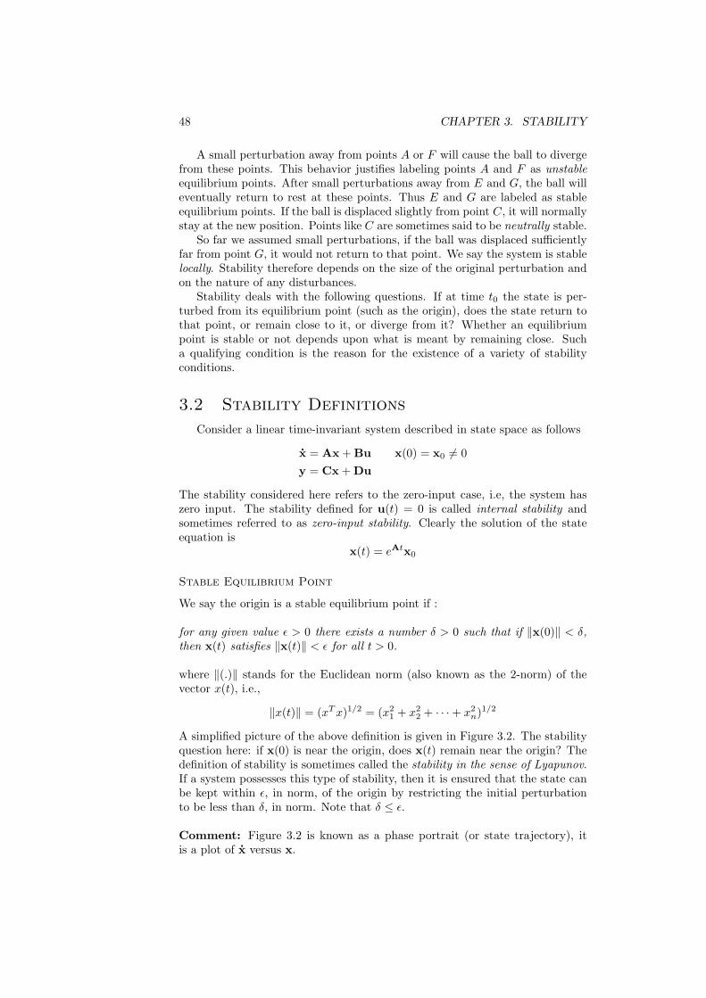
for any given value ε > 0 there exists a number δ > 0 such that if ‖x(0)‖ < δ,then x(t) satisfies ‖x(t)‖ < ε for all t > 0.
where ‖(.)‖ stands for the Euclidean norm (also known as the 2-norm) of thevector x(t), i.e.,
‖x(t)‖ = (xTx)1/2 = (x21 + x2
2 + · · ·+ x2n)1/2
A simplified picture of the above definition is given in Figure 3.2. The stabilityquestion here: if x(0) is near the origin, does x(t) remain near the origin? Thedefinition of stability is sometimes called the stability in the sense of Lyapunov.If a system possesses this type of stability, then it is ensured that the state canbe kept within ε, in norm, of the origin by restricting the initial perturbationto be less than δ, in norm. Note that δ ≤ ε.
Comment: Figure 3.2 is known as a phase portrait (or state trajectory), itis a plot of x versus x.
3.2. STABILITY DEFINITIONS 49
Figure 3.2: Illustration of stable trajectories
Asymptotic Stability
The origin is said to be an asymptotically stable equilibrium point if:
(a) it is stable, and
(b) given δ > 0 such that if ‖x(0)‖ < δ, then x(t) satisfies limt→∞
‖x(t)‖ = 0.

50 CHAPTER 3. STABILITY
Chapter 4Modern Control Design
Classical design techniques are based on either frequency response or the rootlocus. Over the last decade new design techniques has been developed, whichare called modern control methods to differentiate them from classical methods.In this chapter we present a modern control design method known as pole place-ment, or pole assignment. This method is similar to the root-locus design, inthat poles in the closed-loop transfer function may be placed in desired loca-tions. Achievement of suitable pole locations is one of the fundamental designobjectives as this will ensure satisfactory transient response. The placing of allpoles at desired locations requires that all state variables must be measured.In many applications, all needed system variables may not be physically mea-surable or because of cost. In these cases, those system signals that cannot bemeasured must be estimated from the ones that are measured. The estimationof system variables will be discussed later in the chapter.
4.1 State feedback
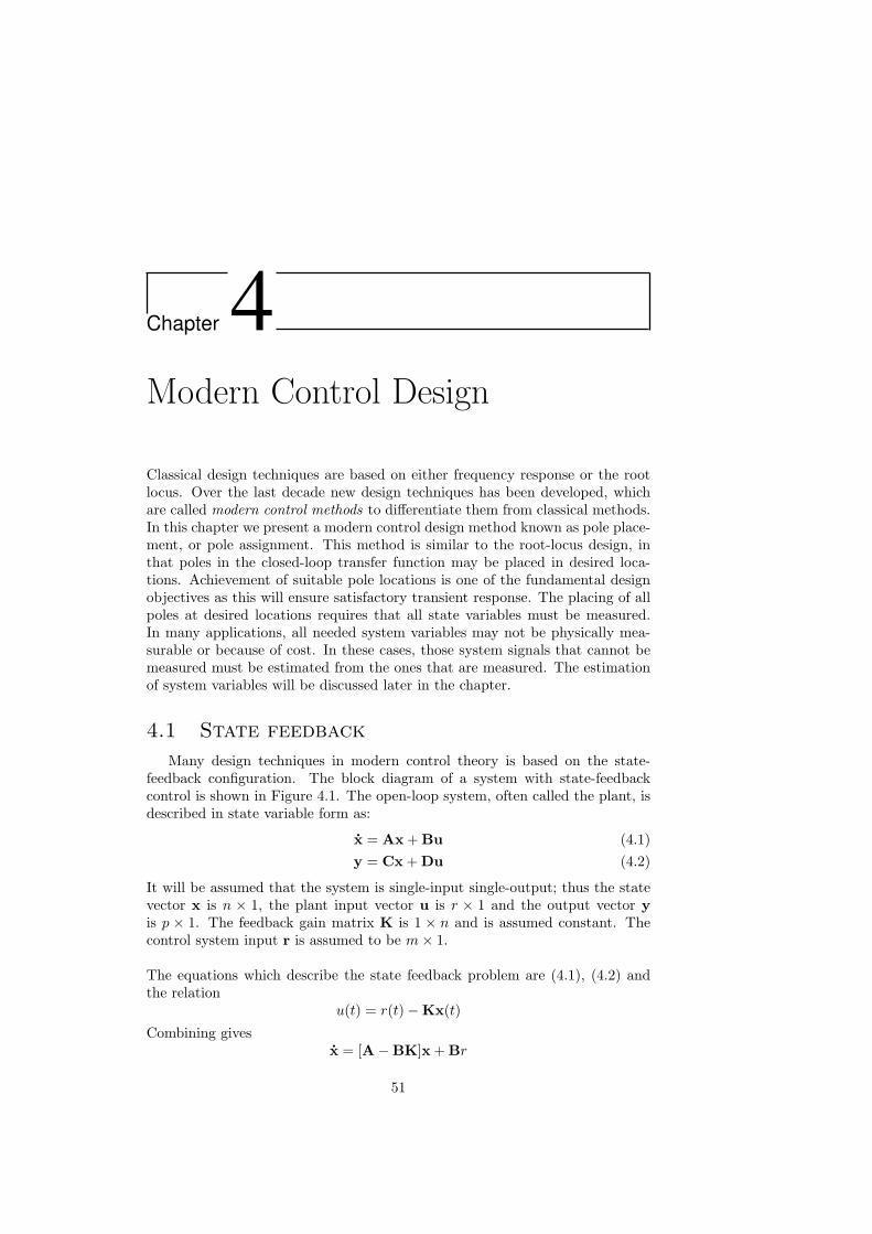
Many design techniques in modern control theory is based on the state-feedback configuration. The block diagram of a system with state-feedbackcontrol is shown in Figure 4.1. The open-loop system, often called the plant, isdescribed in state variable form as:
x = Ax + Bu (4.1)y = Cx + Du (4.2)
It will be assumed that the system is single-input single-output; thus the statevector x is n × 1, the plant input vector u is r × 1 and the output vector yis p × 1. The feedback gain matrix K is 1 × n and is assumed constant. Thecontrol system input r is assumed to be m× 1.
The equations which describe the state feedback problem are (4.1), (4.2) andthe relation
u(t) = r(t)−Kx(t)
Combining givesx = [A−BK]x + Br
51
52 CHAPTER 4. MODERN CONTROL DESIGN
Figure 4.1: State variable feedback system.
andy = [C−DK]x + Dr
With this setup in mind the question is: What changes in overall system char-acteristics can be achieved by the choice of K? Stability of the state feedbacksystem depends on the eigenvalues of (A−BK). Controllability depends on thepair ([A−BK],B). Observability depends on the pair ([A−BK], [C−DK]).
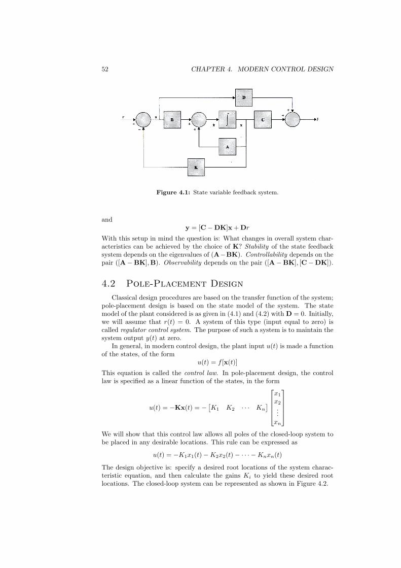
4.2 Pole-Placement Design
Classical design procedures are based on the transfer function of the system;pole-placement design is based on the state model of the system. The statemodel of the plant considered is as given in (4.1) and (4.2) with D = 0. Initially,we will assume that r(t) = 0. A system of this type (input equal to zero) iscalled regulator control system. The purpose of such a system is to maintain thesystem output y(t) at zero.
In general, in modern control design, the plant input u(t) is made a functionof the states, of the form
u(t) = f [x(t)]
This equation is called the control law. In pole-placement design, the controllaw is specified as a linear function of the states, in the form
u(t) = −Kx(t) = −[K1 K2 · · · Kn
]x1
x2
...xn
We will show that this control law allows all poles of the closed-loop system tobe placed in any desirable locations. This rule can be expressed as
u(t) = −K1x1(t)−K2x2(t)− · · · −Knxn(t)
The design objective is: specify a desired root locations of the system charac-teristic equation, and then calculate the gains Ki to yield these desired rootlocations. The closed-loop system can be represented as shown in Figure 4.2.
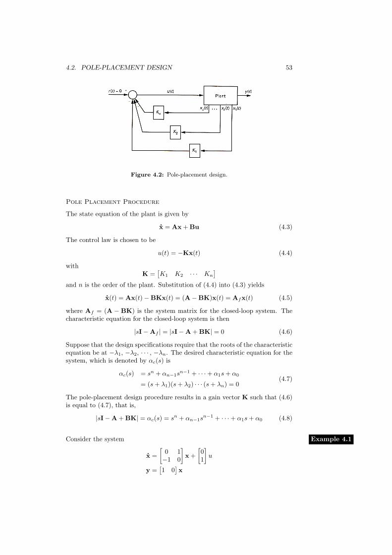
4.2. POLE-PLACEMENT DESIGN 53
Figure 4.2: Pole-placement design.
Pole Placement Procedure
The state equation of the plant is given by
x = Ax + Bu (4.3)
The control law is chosen to be
u(t) = −Kx(t) (4.4)
withK =
[K1 K2 · · · Kn
]and n is the order of the plant. Substitution of (4.4) into (4.3) yields
x(t) = Ax(t)−BKx(t) = (A−BK)x(t) = Afx(t) (4.5)
where Af = (A − BK) is the system matrix for the closed-loop system. Thecharacteristic equation for the closed-loop system is then
|sI−Af | = |sI−A + BK| = 0 (4.6)
Suppose that the design specifications require that the roots of the characteristicequation be at −λ1, −λ2, · · · , −λn. The desired characteristic equation for thesystem, which is denoted by αc(s) is
αc(s) = sn + αn−1sn−1 + · · ·+ α1s+ α0
= (s+ λ1)(s+ λ2) · · · (s+ λn) = 0(4.7)
The pole-placement design procedure results in a gain vector K such that (4.6)is equal to (4.7), that is,
|sI−A + BK| = αc(s) = sn + αn−1sn−1 + · · ·+ α1s+ α0 (4.8)
Consider the system Example 4.1
x =[
0 1−1 0
]x +
[01
]u
y =[1 0
]x
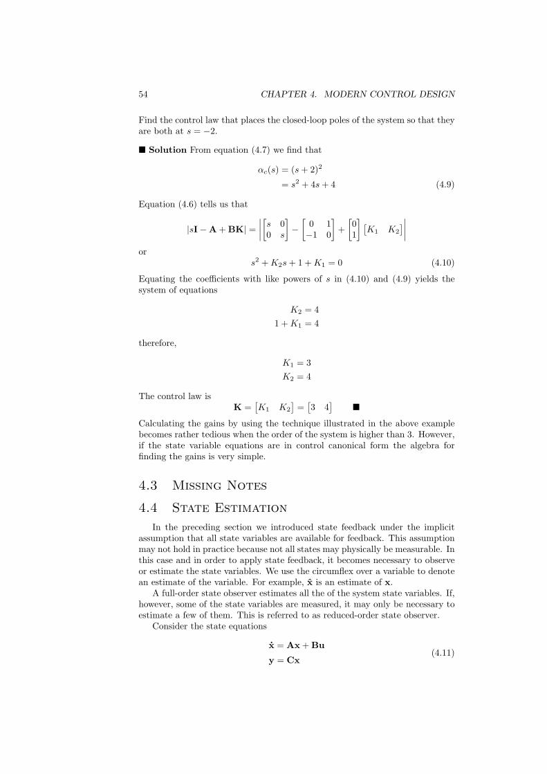
54 CHAPTER 4. MODERN CONTROL DESIGN
Find the control law that places the closed-loop poles of the system so that theyare both at s = −2.
� Solution From equation (4.7) we find that
αc(s) = (s+ 2)2
= s2 + 4s+ 4 (4.9)
Equation (4.6) tells us that
|sI−A + BK| =∣∣∣∣[s 0
0 s
]−[
0 1−1 0
]+[01
] [K1 K2
]∣∣∣∣or
s2 +K2s+ 1 +K1 = 0 (4.10)
Equating the coefficients with like powers of s in (4.10) and (4.9) yields thesystem of equations
K2 = 41 +K1 = 4
therefore,
K1 = 3K2 = 4
The control law isK =
[K1 K2
]=[3 4
]�
Calculating the gains by using the technique illustrated in the above examplebecomes rather tedious when the order of the system is higher than 3. However,if the state variable equations are in control canonical form the algebra forfinding the gains is very simple.
4.3 Missing Notes
4.4 State Estimation
In the preceding section we introduced state feedback under the implicitassumption that all state variables are available for feedback. This assumptionmay not hold in practice because not all states may physically be measurable. Inthis case and in order to apply state feedback, it becomes necessary to observeor estimate the state variables. We use the circumflex over a variable to denotean estimate of the variable. For example, x is an estimate of x.
A full-order state observer estimates all the of the system state variables. If,however, some of the state variables are measured, it may only be necessary toestimate a few of them. This is referred to as reduced-order state observer.
Consider the state equations
x = Ax + Bu
y = Cx(4.11)
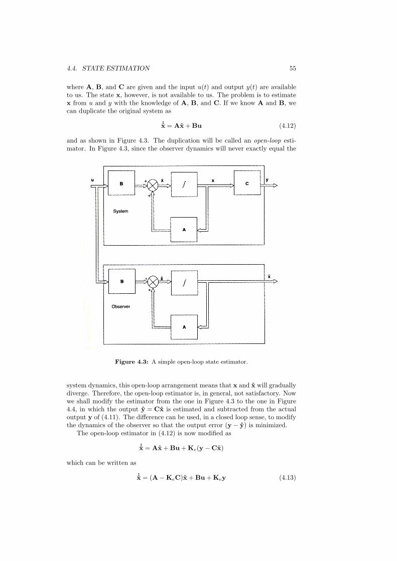
4.4. STATE ESTIMATION 55
where A, B, and C are given and the input u(t) and output y(t) are availableto us. The state x, however, is not available to us. The problem is to estimatex from u and y with the knowledge of A, B, and C. If we know A and B, wecan duplicate the original system as
˙x = Ax + Bu (4.12)
and as shown in Figure 4.3. The duplication will be called an open-loop esti-mator. In Figure 4.3, since the observer dynamics will never exactly equal the
Figure 4.3: A simple open-loop state estimator.
system dynamics, this open-loop arrangement means that x and x will graduallydiverge. Therefore, the open-loop estimator is, in general, not satisfactory. Nowwe shall modify the estimator from the one in Figure 4.3 to the one in Figure4.4, in which the output y = Cx is estimated and subtracted from the actualoutput y of (4.11). The difference can be used, in a closed loop sense, to modifythe dynamics of the observer so that the output error (y − y) is minimized.
The open-loop estimator in (4.12) is now modified as
˙x = Ax + Bu + Ke(y −Cx)
which can be written as
˙x = (A−KeC)x + Bu + Key (4.13)
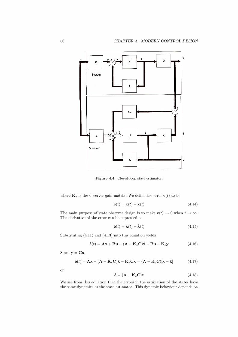
56 CHAPTER 4. MODERN CONTROL DESIGN
Figure 4.4: Closed-loop state estimator.
where Ke is the observer gain matrix. We define the error e(t) to be
e(t) = x(t)− x(t) (4.14)
The main purpose of state observer design is to make e(t) → 0 when t → ∞.The derivative of the error can be expressed as
e(t) = x(t)− ˙x(t) (4.15)
Substituting (4.11) and (4.13) into this equation yields
e(t) = Ax + Bu− (A−KeC)x−Bu−Key (4.16)
Since y = Cx,
e(t) = Ax− (A−KeC)x−KeCx = (A−KeC)[x− x] (4.17)
ore = (A−KeC)e (4.18)
We see from this equation that the errors in the estimation of the states havethe same dynamics as the state estimator. This dynamic behaviour depends on
4.4. STATE ESTIMATION 57
the eigenvalues of (A−KeC). If (A−KeC) is stable, then x → x as t → ∞.Furthermore, these eigenvalues should allow the observer transient response tobe faster than the system itself (typically a factor of 5). In other words, the gainmatrix Ke is chosen to make the dynamics of the estimator faster than those ofthe system.
4.4.1 Estimator Design
We now consider the design of the state estimators. The equation of the esti-mator is given by
˙x = (A−KeC)x + Bu + Key (4.19)
The characteristic equation of the estimator is then
|sI−A + KeC| = 0 (4.20)
Note that this characteristic equation is the same as that of the error in (4.18).As mentioned earlier, one method of designing state estimators is to make theestimator five times faster than the closed-loop system. Hence we choose acharacteristic equation for the estimator, denoted by αe(s), that reflects thedesired speed of response:
αe(s) = (s+ µ1)(s+ µ2) · · · (s+ µn)
= sn + αn−1sn−1 + · · ·+ α1s+ α0 = 0 (4.21)
Then the gain matrix Ke is calculated to satisfy
|sI−A + KeC| = αe(s) (4.22)
The problem of observer design is essentially the same as the regulator poleplacement problem, and similar techniques may be used.
Consider the system Example 4.2
x =[
0 1−1 0
]x +
[01
]u
y =[1 0
]x
this is the same system used in Example 4.1. Compute the estimator gain matrixthat will place the estimator error poles at s = −10 (five times as fast as thecontroller poles selected in example 4.1).
� Solution We are asked to place the two estimator error poles at s = −10.The corresponding characteristic equation is
αe(s) = (s+ 10)2 = s2 + 20s+ 100 (4.23)
From (4.22), we get
|sI−A + KeC| =∣∣∣∣[s 0
0 s
]−[
0 1−1 0
]+[Ke1
Ke2
] [1 0
]∣∣∣∣ = s2 + 20s+ 100
Thuss2 + sKe1 +Ke2 + 1 = s2 + 20s+ 100
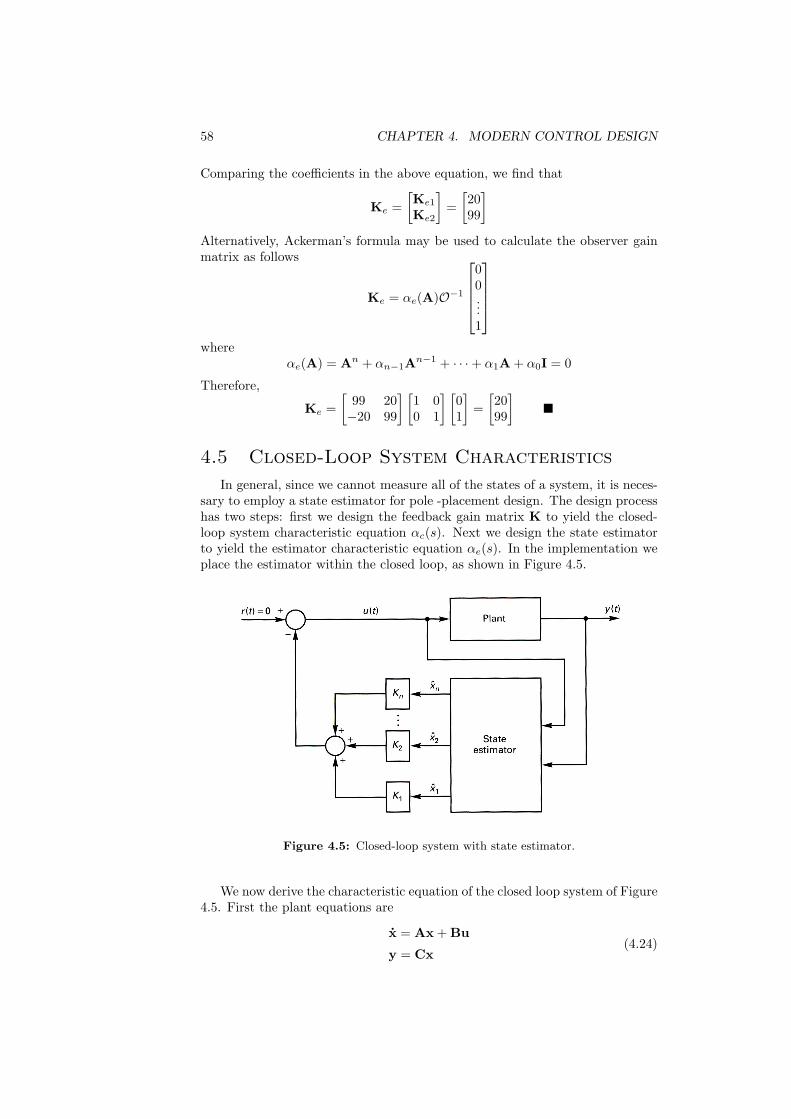
58 CHAPTER 4. MODERN CONTROL DESIGN
Comparing the coefficients in the above equation, we find that
Ke =[Ke1
Ke2
]=[2099
]Alternatively, Ackerman’s formula may be used to calculate the observer gainmatrix as follows
Ke = αe(A)O−1
00...1
where
αe(A) = An + αn−1An−1 + · · ·+ α1A + α0I = 0
Therefore,
Ke =[
99 20−20 99
] [1 00 1
] [01
]=[2099
]�
4.5 Closed-Loop System Characteristics
In general, since we cannot measure all of the states of a system, it is neces-sary to employ a state estimator for pole -placement design. The design processhas two steps: first we design the feedback gain matrix K to yield the closed-loop system characteristic equation αc(s). Next we design the state estimatorto yield the estimator characteristic equation αe(s). In the implementation weplace the estimator within the closed loop, as shown in Figure 4.5.
Figure 4.5: Closed-loop system with state estimator.
We now derive the characteristic equation of the closed loop system of Figure4.5. First the plant equations are
x = Ax + Bu
y = Cx(4.24)
4.5. CLOSED-LOOP SYSTEM CHARACTERISTICS 59
with the control law implemented using observed state variables u(t) = −Kx(t).If the difference between the actual and observed state variables is
e(t) = x(t)− x(t)
thenx(t) = x(t)− e(t) (4.25)
Then, from (4.24) and (4.25),
x = Ax−BK(x− e)
= (A−BK)x + BKe(4.26)
The observer error equation from (4.18) is
e = (A−KeC)e (4.27)
Combining (4.26) and (4.27) gives[x
e
]=
[A−BK BK
0 A−KeC
][x
e
](4.28)
Equation (4.28) describes the closed-loop dynamics of the observed state feed-back control system and because the matrix is block triangular the characteristicequation is
|sI−A + BK||sI−A + KeC| = αc(s)αe(s) = 0 (4.29)
Equation (4.29) shows that the desired closed-loop poles for the control systemare not changed by the introduction of the state observer. The 2n roots of theclosed-loop characteristic equations are then the n roots of the pole-placementdesign plus the n roots of the estimator. Since the observer is normally designedto have a more rapid response than the control system with full order observedstate feedback, the pole-placement roots will dominate.
The closed-loop state equations, with the states chosen as the system statesplus the estimates of those states, will now be derived. From (4.24) and sincethe control law u = −Kx
x = Ax−BKx (4.30)
and from (4.13)
˙x = (A−KeC)x−BKx + KeCx
= (A−KeC−BK)x + KeCx
Thus the closed-loop state equations are then given by[x˙x
]=
[A −BK
KeC A−KeC−BK
][x
x
](4.31)
Consider the system Example 4.3
x =[
0 1−1 0
]x +
[01
]u
y =[1 0
]x
60 CHAPTER 4. MODERN CONTROL DESIGN
In Example 4.1 the gain matrix required to place the poles at s = −2 wascalculated to be
K =[3 4
]and the state-estimator gain matrix was calculated in Example 4.2 to be
Ke =[2099
]The estimator equations are, from (4.13)
˙x = (A−KeC)x + Bu + Key = (A−KeC−BK)x + Key
since u = −Kx. The controller-estimator is then described by the equations
˙x =[−20 1−103 −4
]x +
[2099
]y
u =[−3 −4
]x �
4.5.1 Controller-Estimator Transfer Function
As shown in the example above, the controller-estimator equations are
˙x = (A−KeC−BK)x + Key
u = −Kx
where y is the input and u is the output. Since these equations are in thestandard state-space equations form, we can calculate a transfer function withinput Y (s) and output U(s). Taking the Laplace transform of the controller-estimator equations yields
s ˙X(s) = (A−KeC−BK)X(s) + KeY(s)
U(s) = −KX(s)
and rearranging and solving for U(s), we obtain the transfer function
U(s) = [−K(sI− (A−KeC−BK))−1Ke]Y(s)
For the last example, the controller-estimator transfer function
U(s)Y(s)
=−(456s+ 217)s2 + 24s+ 183
The controller-estimator can be considered as a single transfer function ofGec(s),where
Gec(s) = K(sI− (A−KeC−BK))−1Ke
This configuration is illustrated in Figure 4.6 in which a summing junction hasbeen added to account for the negative sign. The system appears to be thestandard single-loop unity feedback system. The characteristic equation of theclosed-loop system can be expressed as
1 +Gec(s)Gp(s) = 0 (4.32)
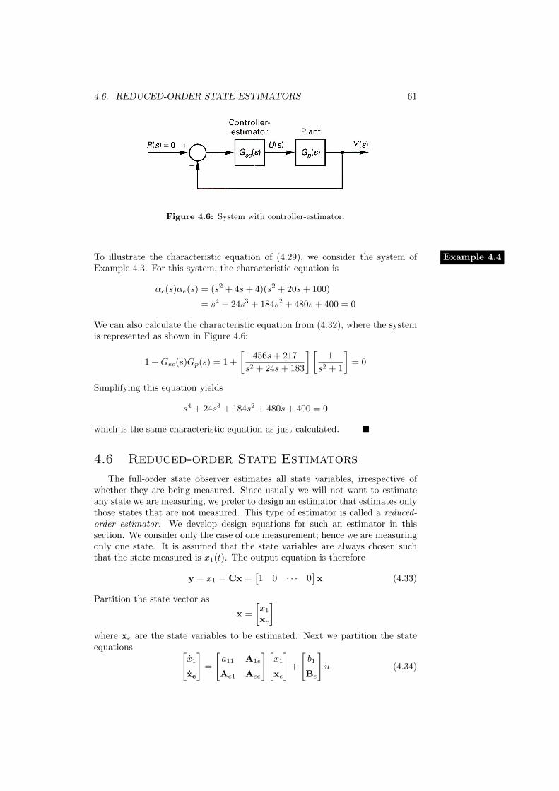
4.6. REDUCED-ORDER STATE ESTIMATORS 61
Figure 4.6: System with controller-estimator.
To illustrate the characteristic equation of (4.29), we consider the system of Example 4.4Example 4.3. For this system, the characteristic equation is
αc(s)αe(s) = (s2 + 4s+ 4)(s2 + 20s+ 100)
= s4 + 24s3 + 184s2 + 480s+ 400 = 0
We can also calculate the characteristic equation from (4.32), where the systemis represented as shown in Figure 4.6:
1 +Gec(s)Gp(s) = 1 +[
456s+ 217s2 + 24s+ 183
] [1
s2 + 1
]= 0
Simplifying this equation yields
s4 + 24s3 + 184s2 + 480s+ 400 = 0
which is the same characteristic equation as just calculated. �
4.6 Reduced-order State Estimators
The full-order state observer estimates all state variables, irrespective ofwhether they are being measured. Since usually we will not want to estimateany state we are measuring, we prefer to design an estimator that estimates onlythose states that are not measured. This type of estimator is called a reduced-order estimator. We develop design equations for such an estimator in thissection. We consider only the case of one measurement; hence we are measuringonly one state. It is assumed that the state variables are always chosen suchthat the state measured is x1(t). The output equation is therefore
y = x1 = Cx =[1 0 · · · 0
]x (4.33)
Partition the state vector as
x =[x1
xe
]where xe are the state variables to be estimated. Next we partition the stateequations [
x1
xe
]=
[a11 A1e
Ae1 Aee
][x1
xe
]+
[b1
Be
]u (4.34)
62 CHAPTER 4. MODERN CONTROL DESIGN
From this equation we write the equation of the states to be estimated,
xe = Ae1x1 + Aeexe + Beu (4.35)
and the equation of the state that is measured
x1 = a11x1 + A1exe + b1u (4.36)
In these equations, xe is unknown and to be estimated, and x1 and u are known.To derive the equations of the estimator, we manipulate (4.35) and (4.36) intothe same form as the plant equations for full state estimation. For full stateestimation,
x = Ax + Bu (4.37)
and for the reduced-order estimator, from (4.35)
xe = Aeexe + [Ae1x1 + Beu] (4.38)
For full state estimationy = Cx (4.39)
and for reduced-order estimator, from (4.36)
[x1 − a11x1 − b1u] = A1exe (4.40)
Comparing (4.37) with (4.38) and (4.39) with (4.40), we see that the equationsare equivalent if we make the following substitutions
x← xeA← Aee
Bu← Ae1x1 + Beu
y← x1 − a11x1 − b1uC← A1e
Making these substitutions into the equation for the full-order estimator,
˙x = (A−KeC)x + Bu + Key
we obtain the equations of the reduced-order estimator
˙xe = (Aee −KeA1e)xe + Ae1y + Beu+ Ke[y − a11y − b1u] (4.41)
where x1 has been replaced with y. The error dynamics are given by
e = xe − ˙xe = (Aee −KeA1e)e (4.42)
Hence the characteristic equation of the estimator and of the errors of estimationare given by
αe(s) = |sI−Aee + KeA1e| = 0 (4.43)
We then choose Ke to satisfy this equation, where we have chosen αe(s) to givethe estimator certain desired dynamics.
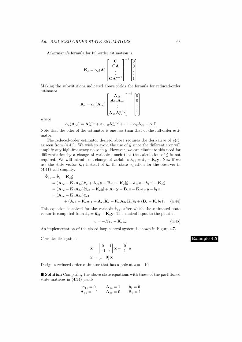
4.6. REDUCED-ORDER STATE ESTIMATORS 63
Ackermann’s formula for full-order estimation is,
Ke = αe(A)
C
CA...
CAn−1
−1
00...1
Making the substitutions indicated above yields the formula for reduced-orderestimator
Ke = αe(Aee)
A1e
A1eAee
...A1eAn−2
ee
−1
00...1
where
αe(Aee) = An−1ee + αn−2An−2
ee + · · ·+ α2Aee + α1I
Note that the oder of the estimator is one less than that of the full-order esti-mator.
The reduced-order estimator derived above requires the derivative of y(t),as seen from (4.41). We wish to avoid the use of y since the differentiator willamplify any high-frequency noise in y. However, we can eliminate this need fordifferentiation by a change of variables, such that the calculation of y is notrequired. We will introduce a change of variables xe1 = xe −Key. Now if weuse the state vector ˙xe1 instead of ˙xe the state equation for the observer in(4.41) will simplify:
˙xe1 = ˙xe −Key
= (Aee −KeA1e)xe + Ae1y + Beu+ Ke[y − a11y − b1u]−Key
= (Aee −KeA1e)[xe1 + Key] + Ae1y + Beu−Kea11y − b1u= (Aee −KeA1e)xe1
+ (Ae1 −Kea11 + AeeKe −KeA1eKe)y + (Be −Keb1)u (4.44)
This equation is solved for the variable xe1, after which the estimated statevector is computed from xe = xe1 + Key. The control input to the plant is
u = −K1y −Kexe (4.45)
An implementation of the closed-loop control system is shown in Figure 4.7.
Consider the system Example 4.5
x =[
0 1−1 0
]x +
[01
]u
y =[1 0
]x
Design a reduced-order estimator that has a pole at s = −10.
� Solution Comparing the above state equations with those of the partitionedstate matrices in (4.34) yields
a11 = 0 A1e = 1 b1 = 0Ae1 = −1 Aee = 0 Be = 1
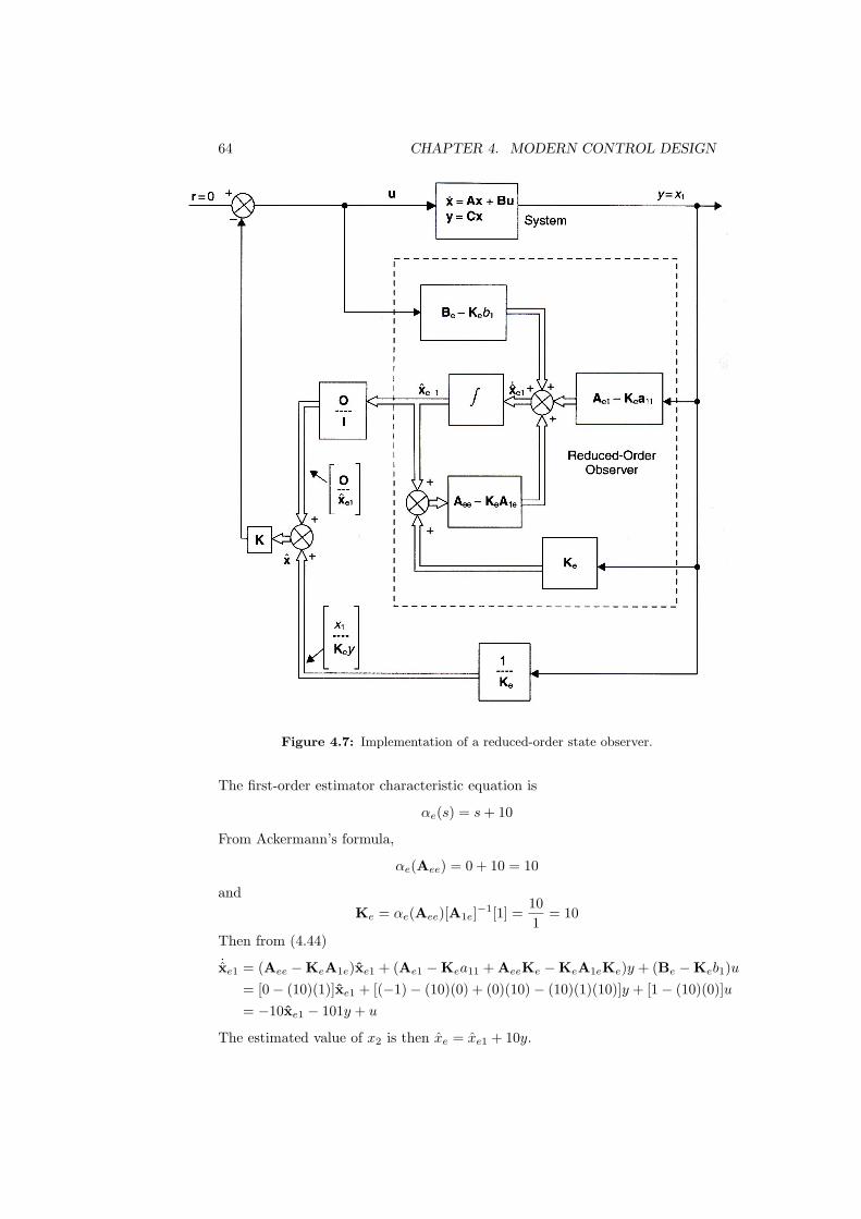
64 CHAPTER 4. MODERN CONTROL DESIGN
Figure 4.7: Implementation of a reduced-order state observer.
The first-order estimator characteristic equation is
αe(s) = s+ 10
From Ackermann’s formula,
αe(Aee) = 0 + 10 = 10
andKe = αe(Aee)[A1e]−1[1] =
101
= 10
Then from (4.44)
˙xe1 = (Aee −KeA1e)xe1 + (Ae1 −Kea11 + AeeKe −KeA1eKe)y + (Be −Keb1)u= [0− (10)(1)]xe1 + [(−1)− (10)(0) + (0)(10)− (10)(1)(10)]y + [1− (10)(0)]u= −10xe1 − 101y + u
The estimated value of x2 is then xe = xe1 + 10y.
4.7. SYSTEMS WITH INPUTS 65
4.6.1 Example page 263
4.7 Systems with Inputs
In the preceding sections only regulator control systems were considered. Aregulator system has no input, and the purpose of the system is to return allstate variables to values of zero when the states have been perturbed. However,many systems require that the system output track an input. For these cases,the design equations for the regulator systems must be modified.
4.7.1 Full State Feedback
We first consider systems with full state feedback. For these systems, the plantis described by
x = Ax + Bu
withu = −Kx
The plant input u is the only function that we can modify; hence the inputfunction r(t) must be added to this function. Therefore, the equation for ubecomes
u = −Kx +Krr
The gain Kr can be determined to satisfy different design criteria. If we expressu as
u = −K1x1 −K2x2 − · · · −Knxn +Krr
we see that one method for choosing Kr is to combine the input r with a linearcombination of the states. For example, suppose that state x1 is the systemoutput that is to track the input r. One logical choice for Kr is then the gainK1, such that u becomes
u = K1[r − x1]−K2x2 − · · · −Knxn