Embed Size (px)
Citation preview

Electromagnetics
Lecture Notes
Dr.K.ParvatisamProfessor
Department Of Electrical And Electronics EngineeringGVP College Of Engineering

Review
Vector Analysis
And
Coordinate Systems

Contents
1 INTRODUCTION 11.1 INTRODUCTION AND MOTIVATION: . . . . . . . . . . . . 11.2 A NOTE TO THE STUDENT: . . . . . . . . . . . . . . . . . 31.3 APPLICATIONS OF ELECTROMAGNETIC FIELD THE-
ORY: . . . . . . . . . . . . . . . . . . . . . . . . . . . . . . . . 7
2 REVIEW 82.1 REVIEWOF COORDINATE SYSTEMS ANDVECTOR CAL-
CULUS: . . . . . . . . . . . . . . . . . . . . . . . . . . . . . . 92.1.1 Learning Objectives . . . . . . . . . . . . . . . . . . . . 92.1.2 Introduction: . . . . . . . . . . . . . . . . . . . . . . . 102.1.3 COORDINATE SYSTEMS: . . . . . . . . . . . . . . . 10
2.1.3.1 RECTANGULAR CARTESIAN COORDINATESYSTEM: . . . . . . . . . . . . . . . . . . . . 11
2.1.3.2 CYLINDRICAL COORDINATE SYSTEM: . 132.1.3.3 SPHERICAL COORDINATE SYSTEM: . . . 19
2.1.4 TRANSFORMATION OF COORDINATES: . . . . . . 252.1.4.1 CARTESIAN TO CYLINDRICAL: . . . . . . 252.1.4.2 CARTESIAN TO SPHERICAL: . . . . . . . 262.1.4.3 CYLINDRICAL TO CARTESIAN: . . . . . . 272.1.4.4 CYLINDRICAL TO SPHERICAL: . . . . . . 272.1.4.5 SPHERICAL TO CARTESIAN: . . . . . . . 282.1.4.6 SPHERICAL TO CYLINDRICAL: . . . . . . 292.1.4.7 COORDINATE TRANSFORMATIONS IN
MATRIX FORM: . . . . . . . . . . . . . . . . 292.2 COORDINATE COMPONENT TRANSFORMATIONS: . . . 32
2.2.0.1 COORDINATE TRANSFORMATION PRO-CEDURE: . . . . . . . . . . . . . . . . . . . . 35
3

CONTENTS
2.3 PARTIAL DERIVATIVES OF UNIT VECTORS: . . . . . . . 352.4 REVIEW OF VECTOR ANALYSIS: . . . . . . . . . . . . . . 40
2.4.1 VECTOR COMPONENTS AND UNIT VECTORS: . 402.4.1.1 THE DOT OR SCALAR PRODUCT: . . . . 422.4.1.2 THE CROSS PRODUCT: . . . . . . . . . . . 44
2.4.2 VECTOR CALCULUS, GRADIENT, DIVERGENCEAND CURL: . . . . . . . . . . . . . . . . . . . . . . . 452.4.2.1 LINE INTEGRALS OF VECTORS: . . . . . 452.4.2.2 SURFACE INTEGRALS OF VECTORS: . . 462.4.2.3 THE GRADIENT . . . . . . . . . . . . . . . 482.4.2.4 PROPERTIES OF GRADIENT OF V (∇V ): 492.4.2.5 EXPRESSION FOR GRADIENT IN DIF-
FERENT COORDINATE SYSTEMS: . . . . 502.4.3 FLUX AND DIVERGENCE OF A VECTOR FIELD: 50
2.4.3.1 SURFACE INTEGRAL AND FLUX OF AVECTOR FIELD: . . . . . . . . . . . . . . . 50
2.4.3.2 THE DIVERGENCE: . . . . . . . . . . . . . 512.4.3.3 EXPRESSION FORDIVERGENCE IN CARTE-
SIAN COORDINATES: . . . . . . . . . . . . 512.4.3.4 PROPERTIES OF DIVERGENCE: . . . . . 532.4.3.5 GEOMETRICAL INTERPRETATION: . . . 532.4.3.6 THE DIVERGENCE THEOREM: . . . . . . 562.4.3.7 PROOF OF DIVERGENCE THEOREM: . . 572.4.3.8 CURL OF A VECTOR AND THE STOKE'S
THEOREM: . . . . . . . . . . . . . . . . . . 572.4.3.9 EXPRESSION FOR CURL IN CARTESIAN
COORDINATES: . . . . . . . . . . . . . . . . 582.4.3.10 STOKE'S THEOREM: . . . . . . . . . . . . 592.4.3.11 PROOF OF STOKE'S THEOREM: . . . . . 602.4.3.12 PROPERTIES OF CURL: . . . . . . . . . . . 612.4.3.13 CLASSIFICATION OF VECTOR FIELDS: . 612.4.3.14 HELMHOLTZ'S THEOREM: . . . . . . . . . 622.4.3.15 VECTOR IDENTITIES: . . . . . . . . . . . . 63
3 STATIC ELECTRIC FIELDS 683.1 COULOMB'S LAW . . . . . . . . . . . . . . . . . . . . . . . . 72
3.1.1 FORCE BETWEEN POINT CHARGES: 723.1.1.1 Elecric charge: . . . . . . . . . . . . . . . . . 72
Dr.K.ParvatisamGVP College of Engineering ( Autonomous )
4

CONTENTS
3.1.2 COULOMB'S LAW IN VECTOR FORM: . . . . . . . 753.1.3 PRINCIPLE OF SUPERPOSITION: . . . . . . . . . . 78
3.2 ELECTRIC FIELD . . . . . . . . . . . . . . . . . . . . . . . . 813.2.1 ELECTRIC FIELD BECAUSE OF CHARGE DIS-
TRIBUTIONS: . . . . . . . . . . . . . . . . . . . . . . 823.2.2 FIELD BECAUSE OF A FINITE LINE CHARGE: . . 843.2.3 CASE I: INFINITE LINE CHARGE: . . . . . . . . . . 863.2.4 CASE II:LOWER END COINCIDING WITH THE
FIELD POINT: . . . . . . . . . . . . . . . . . . . . . . 863.2.5 CASE IV: SEMI- INFINITE LINE: . . . . . . . . . . . 883.2.6 CASE V:SEMI- INFINITE LINE: . . . . . . . . . . . . 883.2.7 CASE VI: SEMI INFINITE LINE: . . . . . . . . . . . 893.2.8 CASE VII:SEMI-INFINITE LINE: . . . . . . . . . . . 903.2.9 CIRCULAR RING OF CHARGE: . . . . . . . . . . . 913.2.10 SURFACE CHARGE DISTRIBUTION: . . . . . . . . 93
3.3 ENERGY AND POTENTIAL . . . . . . . . . . . . . . . . . . 963.3.1 ENERGY EXPENDED INMOVING A POINT CHARGE
IN AN ELECTRIC FIELD: . . . . . . . . . . . . . . . 963.3.2 The LINE INTEGRAL: . . . . . . . . . . . . . . . . . 97
3.3.2.1 THE POTENTIAL FIELD OF A POINT CHARGE: 993.3.2.2 POTENTIAL FIELD BECAUSE OF AGROUP
OF CHARGES: . . . . . . . . . . . . . . . . . 1003.3.2.3 THE POTENTIAL FIELD OF A RING OF
UNIFORM LINE CHARGE DENSITY: . . . 1013.3.2.4 POTENTIAL AT ANY POINT ON THE AXIS
OF UNIFORMLY CHARGED DISC: . . . . . 1033.3.2.5 POTENTIAL AND ELECTRIC FIELD OF
A DIPOLE: . . . . . . . . . . . . . . . . . . . 1053.3.3 ENERGY STORED IN AN ELECTROSTATIC FIELD:109
3.4 GAUSS'S LAW: . . . . . . . . . . . . . . . . . . . . . . . . . . 1153.4.1 ELECTRIC FLUX DENSITY: . . . . . . . . . . . . . 1153.4.2 GAUSS'S LAW: . . . . . . . . . . . . . . . . . . . . . . 119
3.4.2.1 GAUSS'S LAW AND MAXWELL'S EQUA-TION: . . . . . . . . . . . . . . . . . . . . . . 120
3.4.2.2 POTENTIAL GRADIENT: . . . . . . . . . . 1213.4.2.3 Static Electric Field And The Curl: . . . . . . 122
3.4.3 Applications . . . . . . . . . . . . . . . . . . . . . . . . 1243.4.3.1 Electric Forces in Biology . . . . . . . . . . . 124
Dr.K.ParvatisamGVP College of Engineering ( Autonomous )
5

CONTENTS
3.4.3.2 Polarity of Water Molecules . . . . . . . . . . 1253.4.3.3 Earth's Electric Field . . . . . . . . . . . . . 1263.4.3.4 Applications of Conductors . . . . . . . . . . 1273.4.3.5 The Van de Graa� Generator . . . . . . . . . 1293.4.3.6 Xerography . . . . . . . . . . . . . . . . . . . 1303.4.3.7 Laser Printers . . . . . . . . . . . . . . . . . 1323.4.3.8 Ink Jet Printers and Electrostatic Painting . 1333.4.3.9 Smoke Precipitators and Electrostatic Air Clean-
ing . . . . . . . . . . . . . . . . . . . . . . . 134
4 POISSON'S AND LAPLACE'S EQUATIONS: 1374.1 DERIVATION OF LAPLACE'S AND POISSON'S EQUA-
TIONS: . . . . . . . . . . . . . . . . . . . . . . . . . . . . . . 1384.1.1 UNIQUENESS THEOREM: . . . . . . . . . . . . . . . 1404.1.2 EXAMPLES: . . . . . . . . . . . . . . . . . . . . . . . 142
4.2 Electric Dipole . . . . . . . . . . . . . . . . . . . . . . . . . . 1474.2.1 POTENTIAL AND ELECTRIC FIELD OF A DIPOLE:1474.2.2 Torque On A Dipole In an Electric Field . . . . . . . . 1524.2.3 Conductors, Semiconductors, and Insulators . . . . . . 1534.2.4 Conductor free space boundary . . . . . . . . . . . . . 154
5 Polarization 1585.0.1 Linear, Isotropic, And Homogeneous Dielectrics . . . . 1635.0.2 Continuity Equation And Relaxation Time . . . . . . . 1635.0.3 Boundary Conditions: . . . . . . . . . . . . . . . . . . 166
5.0.3.1 Dielectric-Dielectric Boundary Conditions . . 1675.0.3.2 Conductor - Dielectric Boundary: . . . . . . . 1705.0.3.3 Conductor Free space Boundary Conditions . 173
5.1 Capacitance . . . . . . . . . . . . . . . . . . . . . . . . . . . . 1745.1.1 Parallel plate capacitor . . . . . . . . . . . . . . . . . . 1755.1.2 Spherical Capacitor . . . . . . . . . . . . . . . . . . . . 1765.1.3 ENERGY STORED IN AN ELECTROSTATIC FIELD:176
5.2 Current and Current density: . . . . . . . . . . . . . . . . . . 1815.2.1 Continuity Of current: . . . . . . . . . . . . . . . . . . 1835.2.2 Ohm's Law: Point Form . . . . . . . . . . . . . . . . . 1845.2.3 General Expression for Resistance . . . . . . . . . . . . 186
Dr.K.ParvatisamGVP College of Engineering ( Autonomous )
6

CONTENTS
6 THE STEADY MAGNETIC FIELD 1896.0.1 INTRODUCTION: . . . . . . . . . . . . . . . . . . . . 1926.0.2 BIOT-SAVART LAW: . . . . . . . . . . . . . . . . . . 1926.0.3 FIELD BECAUSE OF A FINITE LINE CURRENT: . 1976.0.4 MAGNETIC FIELD AT ANY POINT ON THE AXIS
OF A CIRCULAR CURRENT LOOP: . . . . . . . . . 2026.0.5 MAGNETIC FIELD AT ANY POINT ON THE AXIS
OF A LONG SOLENOID: . . . . . . . . . . . . . . . . 2036.1 MAGNETIC FLUX AND MAGNETIC FLUX DENSITY: . . 205
7 AMPERE'S CIRCUITAL LAW: 2107.0.1 APPLICATIONS: . . . . . . . . . . . . . . . . . . . . . 214
7.0.1.1 INFINITELY LONG FILAMENT: . . . . . . 2147.0.1.2 INFINITELY LONG COAXIAL TRANSMIS-
SION LINE: . . . . . . . . . . . . . . . . . . 2157.0.2 AMPERE'S CIRCUITAL LAW AND MAXWELL'S
EQUATION: . . . . . . . . . . . . . . . . . . . . . . . 2177.0.2.1 Applications Of Ampere's Circuital Law . . . 219
8 MAGNETIC FORCES, MATERIALS, AND INDUCTANCE2238.0.1 FORCE ON A MOVING CHARGE: . . . . . . . . . . 2258.0.2 FORCE ON A DIFFERENTIAL CURRENT ELE-
MENT: . . . . . . . . . . . . . . . . . . . . . . . . . . 2268.0.3 FORCE BETWEENDIFFERENTIAL CURRENT EL-
EMENTS: . . . . . . . . . . . . . . . . . . . . . . . . 2288.0.4 FORCE AND TORQUE ON A CLOSED CIRCUIT: . 232
8.0.4.1 TORQUEONADIFFERENTIAL CURRENTLOOP: . . . . . . . . . . . . . . . . . . . . . 234
8.0.5 Magnetization in Materials: . . . . . . . . . . . . . . . 2388.0.6 Magnetic Boundary Conditions: . . . . . . . . . . . . . 240
9 Magnetic potential 2439.1 Scalar magnetic potential: . . . . . . . . . . . . . . . . . . . . 244
9.1.1 Vector Magnetic Potential: . . . . . . . . . . . . . . . . 246
10 FARADAY'S LAW AND ELECTROMAGNETIC INDUC-TION 251
10.0.1 Transformer e.m.f: . . . . . . . . . . . . . . . . . . . . 257
Dr.K.ParvatisamGVP College of Engineering ( Autonomous )
7

CONTENTS
10.0.2 Motional e.m.f: . . . . . . . . . . . . . . . . . . . . . . 25910.0.3 Displacement Current density: . . . . . . . . . . . . . . 263
Dr.K.ParvatisamGVP College of Engineering ( Autonomous )
8

Chapter 1
INTRODUCTION
1.1 INTRODUCTION AND MOTIVATION:
The focus is on electricity and magnetism, including electric �elds,magnetic �elds, electromagnetic forces, conductors and dielectrics.
Electromagnetics is the study of electric and magnetic phenom-ena caused by electrical charges at rest or in motion.It is one of themost important courses in electrical engineering. It can also beregarded as the study of the interaction between electrical chargesat rest and in motion. It is a branch of electrical engineering orphysics in which electrical and magnetic phenomena are studied.
Mobile phone communication can not be explained by circuittheory concepts alone. The source feeds into an open circuit be-cause the upper tip of the antenna is not connected to any thingphysically, hence no current will �ow and nothing will happen.Thiscannot explain why communication can be established betweenmoving telephone units.
Since the beginning of the twentieth century,the study of elec-tricity and magnetism has been in its mature stage of develop-ment. A steady but ever slower accretion of knowledge has takenplace, so that the graph is asymptotically approaching a plateau.
1

1.1. INTRODUCTION AND MOTIVATION:
When a body of knowledge is in this stage it is called classical.It should not be inferred from this that a classical subject is onethat is at best fruitless. There are still many unsolved problemsin electricity and magnetism
1. Why there are two kinds of charge . Only one kind of grav-itational mass has been found so far. Is mass a simpler andmore fundamental property?
2. Must charge always be associated with mass? Mass alwaysis not associated with charge.
3. Charge is quantized. Why does the minimum quantity ofcharge have the value it does have?
4. Why are electrical forces so overwhelmingly larger than grav-itational forces?
Electrical force is 1043 times the gravitational force.
Dr.K.ParvatisamGVP College of Engineering ( Autonomous )
2

1.2. A NOTE TO THE STUDENT:
The commonly held view by students, expressed vehe-mently , particularly recent survivors of the course is ,that electromagnetics is di�cult, complicated, and a mys-terious discipline. It requires mastery of abstruse mathe-matical techniques,. It also entails juggling a bewilderingvariety of equations , laws and rules, they decide. Evenan intense study has left them with only super�cial graspof the concepts.Few see the beauty of electromagnetics: not many appre-ciate the simplicity and and economy of its fundamen-tal laws. A minority realize its wide ranging utility, thebreadth and scope of its applications. Only a minoritymaster it enough to be able to use its principles to un-derstand or predict the capabilities and limitations of theengineering systems they need to analyze or design.
1.2 A NOTE TO THE STUDENT:
1. Pay particular attention to vector analysis, the mathematicaltool for this course.
2. Do not attempt to memorize too many formulae . Try tounderstand how the formulae are related.
3. Try to identify the key words or terms in a given de�nitionor law
4. Attempt to solve as many problems as possible. Prac-tice is the best way to gain skill
Dr.K.ParvatisamGVP College of Engineering ( Autonomous )
3

1.2. A NOTE TO THE STUDENT:
Your brain should think that what you want to learn is important.It is built to search, scan and wait for something to happen. Itis built that way and helps you to stay alive. You should knowwhat is important and what is not important. So when you wantto learn subject you should know that you have to study andconcentrate whether you like it or not.What does it take to learn something? First you have to get it,and make sure that yo do not forget it. pushing facts mechanicallyinto the head does not help. Learning is a lot more than text ona page. The following are the principles of good learning:
1. Get-and keep - the reader's attention
2. Use a conversational and personalized style
3. Touch their emotions
4. Make it visual
5. Get the learner to think more deeply
Dr.K.ParvatisamGVP College of Engineering ( Autonomous )
4

1.2. A NOTE TO THE STUDENT:
Thinking about thinking:
Real learning takes place , that too quickly and more deeply, if youpay attention to how you pay attention.Think about howyou think. Learn how you learn.Nobody takes a course on learning. You are expected to learn, butrarely taught to learn. The trick is to get the brain think that whatyou are going to learn is important.Ten Principles to bend the Brain:
1. Slow down. If you slow down you understand well. Themore you understand , the less you have to memorize.
2. Do the exercises. Write your own notes. Use pencil.Physical activity while learning can increase learning.
3. Do not Do all Your Learning in One Place. Standup,stretch, move around , change chairs, change rooms.
4. Make what you want to learn the last thing that youread before bed, or at least the last challenging thing.Part of the learning ( especially the long term memory )happens after you put down your book down. Brain needstime for processing, so if you put something new, you loosesome of what you just learned.
5. Drink lots of water. Dehydration decreases cognitive func-tion.
6. Talk about it and also loudly. Better try to explain it tosomeone else loudly.
7. Listen to your brain . Know when the brain is overloaded.
8. Feel something. Get involved. Feeling nothing at all is bad.
9. There are no dumb questions. Sometimes the questionsare more useful than the answers.
10. Shut your mouth and listen, suspending your judg-ment, when you want to learn something from some otherperson.
Dr.K.ParvatisamGVP College of Engineering ( Autonomous )
5

1.2. A NOTE TO THE STUDENT:
• Review the previous lecture
• Ask questions if needed
• Do suggested course activities
Dr.K.ParvatisamGVP College of Engineering ( Autonomous )
6

1.3. APPLICATIONS OF ELECTROMAGNETIC FIELD THEORY:
1.3 APPLICATIONS OF ELECTROMAGNETIC
FIELD THEORY:
1. Microwaves
2. Antennas
3. Electrical Machines
4. Satellite Communications
5. Plasmas
6. Fiber Optics
7. Bio-electromagnetics
8. Nuclear Research
9. Electro mechanical energyconversion
10. Radar
11. Meteorology
12. Remote sensing
13. Induction Heating
14. Surface Hardening, Dielec-tric Heating
15. Enhance Vegetable Tasteby Reducing Acidity
16. Speed baking Of Bread
17. Physics based signal pro-cessing
18. Computer chip design
19. lasers
20. EMC/EMI Analysis
Dr.K.ParvatisamGVP College of Engineering ( Autonomous )
7

8

2.1. REVIEW OF COORDINATE SYSTEMS AND VECTOR
CALCULUS:
Chapter 2
REVIEW
2.1 REVIEW OF COORDINATE SYSTEMS
AND VECTOR CALCULUS:
2.1.1 Learning Objectives'
&
$
%
• To be able to describe the three coordinate systems we usein describing �elds: Cartesian, cylindrical, and spherical.
• To be able to manipulate vectors and perform common oper-ations with them: decomposition, addition, subtraction, dotproducts, and cross products.
• To be able to describe the fundamental meaning of integra-tion in one, two, and three dimensions as a summation pro-cess.
• To be able to describe the fundamental meaning of di�eren-tiation.
• To be able to recognize situations where Taylor series shouldbe used, and to be able to demonstrate that you can carryout a Taylor series expansion to �rst order.
• To be able to understand the signi�cance of the gradient,divergence , and curl operations and prove divergence andStoke's therorems.
Dr.K.ParvatisamGVP College of Engineering ( Autonomous )
9

2.1. REVIEW OF COORDINATE SYSTEMS AND VECTOR
CALCULUS:
2.1.2 Introduction:
In order to be able to handle with ease many of the elctromag-netic quantities which are vectors, we must choose a coordinatesystem. we will see how to resolve a given vector into componentsin these coordinate systems and how to transform a vector fromone coordinate system into another.
We will discuss the signi�cance of the gradient, divergence ,and curl operations and prove divergence and Stoke's theorems.
This chapter discusses about vector analysis which consists of
1. Vector algebra - addition, subtraction , and multiplication ofvectors
2. Vector calculus - di�erentiation and integration of vectors;gradient,divergence, and curl operations.
This chapter discusses also about
1. Orthogonal coordinate systems- Cartesian, Cylindrical, andspherical coordinates
2.1.3 COORDINATE SYSTEMS:
The dimension of space comes from nature. The measurementof space comes from us. The laws of electromagnetics are inde-pendent of a particular coordinate system. However applicationof the laws to the solution of a particular problem imposes theneed to use a suitable coordinate system. It is the shape of theboundary that determines the most suitable coordinate system touse in its solution. To represent points in space we need a co-ordinate system. The co-ordinate system may be orthogonal ornon-orthogonal. Coordinate systems can also be right handed or
Dr.K.ParvatisamGVP College of Engineering ( Autonomous )
10

2.1. REVIEW OF COORDINATE SYSTEMS AND VECTOR
CALCULUS:
left handed. We discuss only right handed, orthogonal coordinatesystems. The coordinate systems discussed are three dimensionalcoordinate systems. The coordinate systems are de�ned by a setof planes and/or surfaces. A coordinate system de�nes a set ofthree reference directions at each and every point in space.Theorigin of the coordinate system is the reference point relative towhich we locate every other point in space. A position vectorde�nes the position of a point in space relative to the origin.Thethree reference directions are referred to as coordinate directions.Unit vectors along the coordinate directions are called base vec-tors. In any three dimensional coordinate system , an arbitraryvector can be expressed in terms of a superposition of the threebase vectors. Di�erent coordinate systems are di�erent ways tomeasure space.
2.1.3.1 RECTANGULAR CARTESIAN COORDINATE SYSTEM:
The rectangular Cartesian coordinate system is described by threeplanes which are mutually perpendicular to each other. The threeplanes intersect at a point 'O' which is called the origin of thecoordinate system. There are three coordinate axes which areusually denoted by x,y,z. Values of x,y,z are measured from theorigin. The three planes are
• x= constant plane ie yz plane
• y= constant plane ie xz plane
• z= constant plane ie xy plane
Dr.K.ParvatisamGVP College of Engineering ( Autonomous )
11

2.1. REVIEW OF COORDINATE SYSTEMS AND VECTOR
CALCULUS:
A point in rectangular coordinate system is de�ned by (x, y, z).The limits for the coordinates are
−∞ ≤ x ≤ ∞ (2.1)
−∞ ≤ y ≤ ∞ (2.2)
−∞ ≤ z ≤ ∞ (2.3)
The unit or base vectors are ax, ay, az. The following relationshold for the dot and cross products of the unit vectors
ax × ay = az (2.4)
ay × az = ax (2.5)
az × ax = ay (2.6)
ax • ay = 0 (2.7)
ay • az = 0 (2.8)
az • ax = 0 (2.9)
The di�erential length element is given by
dl = dxax + dyay + dzaz (2.10)
The di�erential area elements are
dsrec =
dxdyaz
dydzax
dzdxay
the di�erential volume element is
dv = dxdydz (2.11)
Dr.K.ParvatisamGVP College of Engineering ( Autonomous )
12

2.1. REVIEW OF COORDINATE SYSTEMS AND VECTOR
CALCULUS:
Figure 2.1: Cartesian rectangular coordinate system
2.1.3.2 CYLINDRICAL COORDINATE SYSTEM:
The cylindrical coordinate system is also de�ned by three mutuallyorthogonal surfaces. They are a cylinder and two planes. One ofthe planes is the same as the z = constant plane in the Cartesiancoordinate system. The second plane is orthogonal to the z =constant plane and hence contains the z−axis . it makes an angleφ with the xz−plane. This plane is de�ned by φ = constant.Thethird one is a cylinder whose axis is the z axis and has a radius ρ =constant from the z− axis. So a point in cylindrical coordinatesis de�ned by (ρ, φ, z). The limits for the coordinates are
0 ≤ ρ ≤ ∞
0 ≤ φ ≤ 2π
−∞ ≤ z ≤ ∞
(2.12)
The unit or base vectors are aρ, aφand az . The following rela-
Dr.K.ParvatisamGVP College of Engineering ( Autonomous )
13

2.1. REVIEW OF COORDINATE SYSTEMS AND VECTOR
CALCULUS:
tions hold for the dot and cross products
aρ × aφ = az
aφ × az = aρ
az × aρ = aφ
(2.13)
aρ • aφ = 0
aφ • az = 0
az • aρ = 0
(2.14)
The vector di�erential length element is given by
dlcy = dρaρ + ρdφaφ + dzaz (2.15)
The three di�erential area elements are
dscy =
(ρdφ) (dz) aρ
(dz) (dρ) aφ
(dρ) (ρdφ) az
(2.16)
See the �g. The area is ρdφdzaρ
Dr.K.ParvatisamGVP College of Engineering ( Autonomous )
14

2.1. REVIEW OF COORDINATE SYSTEMS AND VECTOR
CALCULUS:
Figure 2.2: Cylindrical area
See the �g. below. The area is dρdzaφ
Dr.K.ParvatisamGVP College of Engineering ( Autonomous )
15

2.1. REVIEW OF COORDINATE SYSTEMS AND VECTOR
CALCULUS:
Figure 2.3: Cylindrical area element
See the �g. below. The area element is ρdρdφaz
Dr.K.ParvatisamGVP College of Engineering ( Autonomous )
16

2.1. REVIEW OF COORDINATE SYSTEMS AND VECTOR
CALCULUS:
Figure 2.4: Cylindrical area element
The di�erential volume element is given by
dvcy = ρdρdφdz (2.17)
See �g
Dr.K.ParvatisamGVP College of Engineering ( Autonomous )
17

2.1. REVIEW OF COORDINATE SYSTEMS AND VECTOR
CALCULUS:
Figure 2.5: Volume element in cylindrical coordinate system
Another view of cylindrical coordinate system:
Figure 2.6: Cylindrical coordinate system
Dr.K.ParvatisamGVP College of Engineering ( Autonomous )
18

2.1. REVIEW OF COORDINATE SYSTEMS AND VECTOR
CALCULUS:
A third view of cylindrical coordinate system:
Figure 2.7: Cylindrical coordinate system
2.1.3.3 SPHERICAL COORDINATE SYSTEM:
It is de�ned by two surfaces and one plane. The surfaces are asphere and a cone. The plane is φ = constant plane. The sphereis centered at the origin and has a radius r = constant . The conehas its vertex at the origin and its surface is symmetrical aboutthe z − axis, so that the angle θ which the conical surface makeswith the z− axis is constant. A point in spherical co-ordinates isrepresented by p = (r, θ and φ) . The limits for the coordinatesare
Dr.K.ParvatisamGVP College of Engineering ( Autonomous )
19
2.1. REVIEW OF COORDINATE SYSTEMS AND VECTOR
CALCULUS:
0 ≤ r ≤ ∞
0 ≤ θ ≤ π
0 ≤ φ ≤ 2π
(2.18)
The di�erential length is given by
dlsph = drar + rdθaθ + rsinθdφaφ (2.19)
The di�erential area element is given by
dssph =
rdrdθaφ
r2 sin θdθdφar
r sin θdrdφaθ
(2.20)
The di�erential volume element is given by
dvsph = r2 sin θdrdθdφ (2.21)
See the �g. below for the volume and area elements
Dr.K.ParvatisamGVP College of Engineering ( Autonomous )
20

2.1. REVIEW OF COORDINATE SYSTEMS AND VECTOR
CALCULUS:
Figure 2.8: Spherical volume and area elements
Spherical coordinate system
Dr.K.ParvatisamGVP College of Engineering ( Autonomous )
21

2.1. REVIEW OF COORDINATE SYSTEMS AND VECTOR
CALCULUS:
Figure 2.9:
Another view of the spherical coordinate system:
Figure 2.10: Spherical coordinate system
Dr.K.ParvatisamGVP College of Engineering ( Autonomous )
22

2.1. REVIEW OF COORDINATE SYSTEMS AND VECTOR
CALCULUS:
Cartesian Cylindrical Spherical
OrthogonalSurfaces
Three Planes A Cylinder and two Planes A Sphere , a Cone , and a Plane
Geometry Fig. Fig. Fig.
Coordinates x, y, z ρ, φ, z r, θ, φ
Limits OfCoordinates
−∞ ≤ x ≤ ∞
−∞ ≤ y ≤ ∞
−∞ ≤ z ≤ ∞
0 ≤ ρ ≤ ∞
0 ≤ φ ≤ 2π
−∞ ≤ z ≤ ∞
0 ≤ r ≤ ∞
0 ≤ θ ≤ π
0 ≤ φ ≤ 2π
Di�erentialLengthelements
dxax + dyay + dzaz dρaρ + ρdφaφ + dzaz drar + rdθaθ + r sin θdφaφ
Di�erentialAreas
dxdyaz
dydzax
dzdxay
ρdρdφaz
ρdφdzaρ
dρdzaφ
rdrdθaφ
r2 sin θdθdφar
r sin θdrdφaθ
Di�erentialvolume
dxdydz ρdρdφdz r2 sin θdrdθdφ
Table 2.1: Summary of Cartesian, Cylindrical and spherical coordinate sys-tems
Dot products of vectors at a point (r, θ, φ)
Dr.K.ParvatisamGVP College of Engineering ( Autonomous )
23

2.1. REVIEW OF COORDINATE SYSTEMS AND VECTOR
CALCULUS:
ax ay az aρ aφ ar aθ aφ
ax 1 0 0 cosφ − sinφ sin θ cosφ cos θ cosφ − sinφ
ay 1 0 sinφ cosφ sin θ sinφ cos θ cosφ cosφ
az 1 0 0 cos θ − sin θ 0
aρ 1 0 sin θ cos θ 0
aφ 1 0 0 1
ar 1 0 0
aθ 1 0
Table 2.2: Dot products of unit vectors at a point
Cross product of unit vectors at a point (r, θ, φ)
Dr.K.ParvatisamGVP College of Engineering ( Autonomous )
24

2.1. REVIEW OF COORDINATE SYSTEMS AND VECTOR
CALCULUS:
ax ay az aρ aφ ar aθ
ax 0 az −ay sinφaz cosφaz sin θ sinφaz − cos θay cos θ sinφaz + sin θay
ay 0 ax − cosφaz sinφaz − sin θ cosφaz + cos θax − cos θ cosφaz − sin θax
az 0 aφ −aρ sin θaφ cos θaφ
aρ 0 az − cos θaφ sin θaφ
aφ 0 − sin θaz + cos θaρ − cos θaz − sin θaρ
ar 0 aφ
aθ 0
Table 2.3: Cross products of unit vectors at a point
2.1.4 TRANSFORMATION OF COORDINATES:
2.1.4.1 CARTESIAN TO CYLINDRICAL:
If a vector is expressed in Cartesian coordinates as A = Axax +Ayay + Azaz
x = ρ cosφ
y = ρ sinφ
z = z
(2.22)
Dr.K.ParvatisamGVP College of Engineering ( Autonomous )
25

2.1. REVIEW OF COORDINATE SYSTEMS AND VECTOR
CALCULUS:
ρ =√x2 + y2
φ = arctan yx
z = z
(2.23)
then the equivalent vector in cylindrical coordinates is given by
Aρ = Ax cosφ+ Ay sinφ
Aφ = −Ax sinφ+ Ay cosφ
Az = Az
(2.24)
2.1.4.2 CARTESIAN TO SPHERICAL:
Ar = Ax sin θ cosφ+ Ay sin θ sinφ+ Az cos θ
Aθ = Ax cos θ cosφ+ Ay cos θ sinφ− Az sin θ
Aφ = −Ax sinφ+ Ay cosφ
(2.25)
r =√x2 + y2 + z2
θ = arccos z√x2+y2+z2
φ = arctan yx
(2.26)
Dr.K.ParvatisamGVP College of Engineering ( Autonomous )
26

2.1. REVIEW OF COORDINATE SYSTEMS AND VECTOR
CALCULUS:
x = r sin θ cosφ
y = r sin θ sinφ
z = r cos θ
(2.27)
2.1.4.3 CYLINDRICAL TO CARTESIAN:
x = ρ cosφ
y = ρ sinφ
z = z
(2.28)
Ax =Aρx−Aφy√
x2+y2
Ay =Aρy+Aφx√
x2+y2
Az = Az
(2.29)
2.1.4.4 CYLINDRICAL TO SPHERICAL:
r =√ρ2 + z2
θ = arctan ρz
φ = φ
(2.30)
Dr.K.ParvatisamGVP College of Engineering ( Autonomous )
27

2.1. REVIEW OF COORDINATE SYSTEMS AND VECTOR
CALCULUS:
Ar = Aρ sin θ + Az cos θ
Aθ = Aρ cos θ − Az sin θ
Aφ = Aφ
(2.31)
where
cos θ = z√ρ2+z2
sin θ = ρ√ρ2+z2
(2.32)
2.1.4.5 SPHERICAL TO CARTESIAN:
x = r sin θ cosφ
y = r sin θ cosφ
z = r cos θ
(2.33)
Ax =Arx√x2+y2+Aθxz−Aφy
√x2+y2+z2√
(x2+y2)(x2+y2+z2)
Ay =Ary√x2+y2+Aθyz+Aφx
√x2+y2+z2√
(x2+y2)(x2+y2+z2)
Az =Arz−Aθ
√x2+y2√
x2+y2+z2
(2.34)
Dr.K.ParvatisamGVP College of Engineering ( Autonomous )
28

2.1. REVIEW OF COORDINATE SYSTEMS AND VECTOR
CALCULUS:
2.1.4.6 SPHERICAL TO CYLINDRICAL:
ρ = r sin θ
φ = φ
z = r cos θ
(2.35)
Aρ = Arr sin θ+Aθz√r2 sin2 θ+z2
Aφ = Aφ
Az = Arz−Aθr sin θ√r2 sin2 θ+z2
(2.36)
2.1.4.7 COORDINATE TRANSFORMATIONS INMATRIX FORM:
Rectangular to cylindrical:Aρ
Aφ
Az
=
cosφ sinφ 0
− sinφ cosφ 0
0 0 1
Ax
Ay
Az
(2.37)
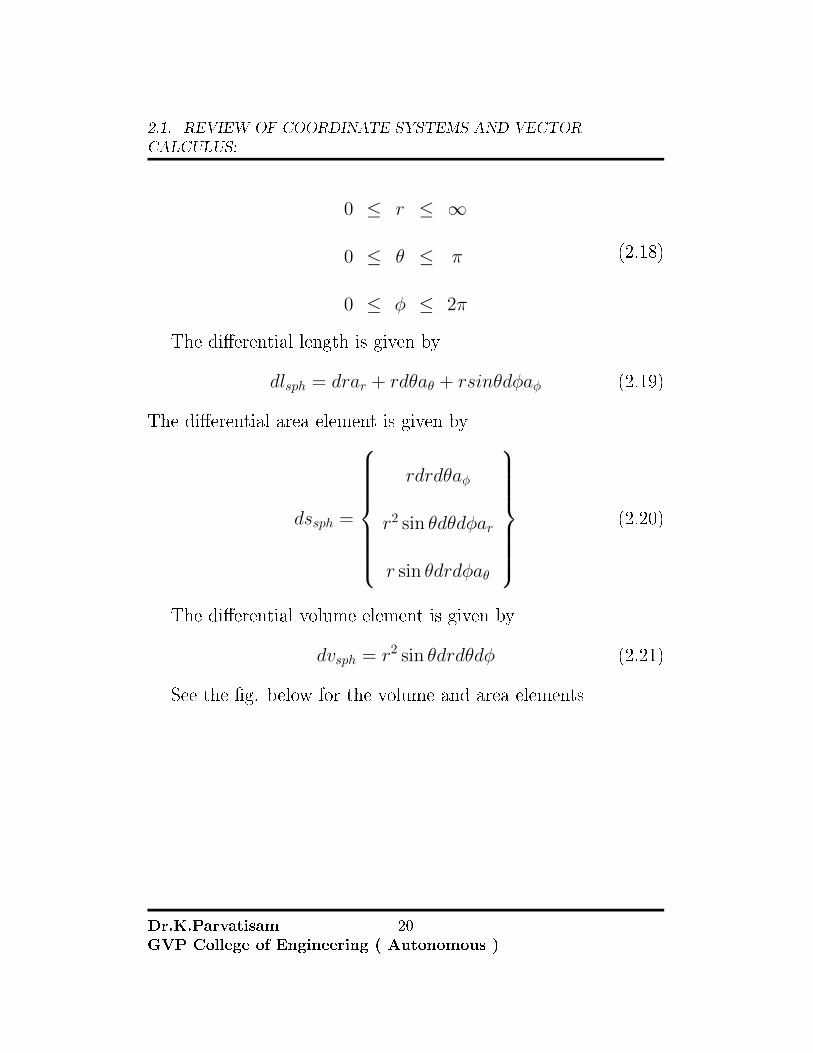
Rectangular to Spherical:
Dr.K.ParvatisamGVP College of Engineering ( Autonomous )
29
2.1. REVIEW OF COORDINATE SYSTEMS AND VECTOR
CALCULUS:
Ar
Aθ
Aφ
=
sin θ cosφ sin θ sinφ cos θ
cos θ cosφ − cos θ sinφ − sin θ
− sinφ cosφ 0
Ax
Ay
Az
(2.38)
Cylindrical to rectangular:
Ax
Ay
Az
=
x√x2+y2
− y√x2+y2
0
y√x2+y2
x√x2+y2
0
0 0 1
Aρ
Aφ
Az
(2.39)
Cylindrical to spherical:Ar
Aθ
Aφ
=
sin θ 0 cos θ
cos θ 0 − sin θ
0 1 0
Aρ
Aφ
Az
(2.40)
Spherical to rectangular:
Dr.K.ParvatisamGVP College of Engineering ( Autonomous )
30

2.1. REVIEW OF COORDINATE SYSTEMS AND VECTOR
CALCULUS:
Ax
Ay
Az
=
sin θ cosφ sin θ sinφ cos θ
cos θ cosφ − cos θ sinφ 0− sin θ
− sinφ cosφ 0
Ar
Aθ
Aφ
(2.41)
Spherical to cylindrical:Aρ
Aφ
Az
=
ρ√ρ2+z2
z√ρ2+z2
0
0 0 1
z√ρ2+z2
ρ√ρ2+z2
0
Ar
Aθ
Aφ
(2.42)
Dr.K.ParvatisamGVP College of Engineering ( Autonomous )
31
2.2. COORDINATE COMPONENT TRANSFORMATIONS:
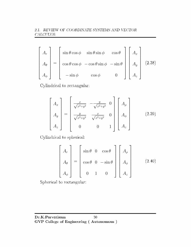
2.2 COORDINATE COMPONENT TRANSFOR-
MATIONS:
Rectangular to Cylindrical
x = ρ cosφ
y = ρ sinφ
z = zAρ
Aφ
Az
=
cosφ sinφ 0
− sinφ cosφ 0
0 0 1
Ax
Ay
Az
Rectangular to Spherical
x = r sin θ cosφ
y = r sin θ sinφ
z = r cos θAr
Aθ
Aφ
=
sin θ cosφ sin θ sinφ cos θ
cos θ cosφ cos θ sinφ − sin θ
− sinφ cosφ 0
Ax
Ay
Az
Table 2.4: Rectangular to cylindrical and spherical
Dr.K.ParvatisamGVP College of Engineering ( Autonomous )
32

2.2. COORDINATE COMPONENT TRANSFORMATIONS:
Cylindrical to Rectangular:
ρ =√x2 + y2
φ = arctany
xz = z
Ax
Ay
Az
=
x√x2+y2
− y√x2+y2
0
y√x2+y2
x√x2+y2
0
0 0 1
Aρ
Aφ
Az
Cylindrical to spherical:
ρ = r sin θ
φ = φ
z = r cos θAr
Aθ
Aφ
=
sin θ 0 cos θ
cos θ 0 − sin θ
0 1 0
Aρ
Aφ
Az
Table 2.5: Cylindrical to Rectangular and Spherical
Dr.K.ParvatisamGVP College of Engineering ( Autonomous )
33

2.2. COORDINATE COMPONENT TRANSFORMATIONS:
Spherical to Rectangular:
r =√x2 + y2 + z2
θ = arctan
√x2 + y2
z
φ = arctany
xAx
Ay
Az
=
x√
x2+y2+z2xz√
x2+y2√x2+y2+z2
− y√x2+y2
y√x2+y2+z2
yz√x2+y2
√x2+y2+z2
x√x2+y2
z√x2+y2+z2
−√x2+y2√
x2+y2√x2+y2+z2
0
Ar
Aθ
Aφ
Spherical to Cylindrical:
r =√ρ2 + z2
θ = arctanρ
zφ = φ
Aρ
Aφ
Az
=
ρ√ρ2+z2
z√ρ2+z2
0
0 0 1
z√ρ2+z2
− ρ√ρ2+z2
0
Ar
Aθ
Aφ
Table 2.6: Spherical to Rectangular and Cylindrical
Dr.K.ParvatisamGVP College of Engineering ( Autonomous )
34

2.3. PARTIAL DERIVATIVES OF UNIT VECTORS:
2.2.0.1 COORDINATE TRANSFORMATION PROCEDURE:
1. Transform the component scalars into the new coordinatesystem
2. Insert the component scalars into the coordinate transforma-tion matrix and evaluate
3. steps 1 and 2 can be performed in either order
2.3 PARTIAL DERIVATIVES OF UNIT VEC-
TORS:
(All derivatives not listed in the table are zero)
∂x ∂y ∂z ∂ρ ∂φ ∂θ
∂aρ/ − sinφρaφ
cosφρaφ 0 0 aφ 0
∂aφ/sinφρaρ − cosφ
ρar 0 0 −aρ 0
∂ar/1r(− sinφaφ + cosφaφ) 1
r(cosφaφ + cos θ sinφaθ)
− sin θraθ
cos θraθ sin θaφ aθ
∂aθ/cot θr
(− sinφaφ − sin θ cosφar)cot θr
(cosφaφ − sin θ sinφarsin θrar
− cos θr
ar cos θaφ −ar
Table 2.7: Partial deviates of unit vectors
Example:
1. Transform each of the following vectors to cylindrical coor-dinates at the point speci�ed
(a) 5ax at P (ρ = 4, φ = 1200, z = 2)
Dr.K.ParvatisamGVP College of Engineering ( Autonomous )
35

2.3. PARTIAL DERIVATIVES OF UNIT VECTORS:
(b) 5ax at Q(x = 3, y = 4, z = −1)
(c) A = 4ax − 2ay − 4az at Q(2, 3, 5)
Ans:a) The ρ component is 5ax • aρ = 5 cosφ
The φ component is 5ax • aφ = −5 sinφThe z component is 5ax • az = 0
so P = 5 cosφaρ − 5 sinφaφwhere φ = 1200
Pcyl = −2.5aρ − 4.33aφ
b) Q = 5 cosφaρ − 5 sinφaφ where φ = arctan 43 = 53.130
Q = 3aρ − 4aφ
c) A = 4ax− 2ay − 4az.Transforming to cylindrical coordi-nates the components are
Aρ = 4 cosφ− 2 sinφ
Aφ = −4 sinφ− 2 cosφ
Az = −4
φ = arctan 32 = 56.30 cosφ =
0.55, sinφ = 0.832
Acy = 0.54aρ − 4.44aφ − 4az
Dr.K.ParvatisamGVP College of Engineering ( Autonomous )
36

2.3. PARTIAL DERIVATIVES OF UNIT VECTORS:
Problems: Coordinate Transformations
1. Transform the following vector
G =xz
yax (2.43)
into spherical coordinates.
2. Transform the vectorB = yax − xay + zaz into cylindricalcoordinates.
3. Give
(a) The cartesian coordinates of the point C(ρ = 4.4, φ =−1150, z = 2)
(b) The cylindrical coordinates of the pointD(x = −3.1, y =2.6, z = −3)
(c) Specify the distance from C to D
4. Transform to cylindrical coordinates
(a) F = 10ax − 8ay + 6az , at point P (10,−8, 6)
(b) G = (2x+ y)ax − (y − 4x)ay at point Q(ρ, φ, z)
(c) Give the cartesian components of the vectorH = 20aρ−10aφ + 3az at P (x = 5, y = 2, z = −1)
5. Given the two points C(−3, 2, 1) and D(r = 5, θ = 200, φ =−700), �nd
(a) The spherical coordinates of C
(b) The cartesian coordinates of D
(c) the distance from C to D
Dr.K.ParvatisamGVP College of Engineering ( Autonomous )
37

2.3. PARTIAL DERIVATIVES OF UNIT VECTORS:
6. Transform the following vectors to spherical coordinates atthe points given
(a) 10ax at P (x = 3, y = 2, z = 4)
(b) 10ay at Q(ρ = 5, φ = 300.z = 4)
(c) 10az at M(r = 4, θ = 1100, φ = 1200)
7. Given points A(ρ = 5, φ = 700, z = −3) and B(ρ = 2, φ =−300, z = 1) �nd
(a) A unit vector in cartesian coordinates at A directed to-wards B
(b) A unit vector in cylindrical coordinates at A directedtowards B
(c) A unit vector in cylindrical coordinates at B directedtowards A
8. Express the vector �eld D = (x2 + y2)−1(xax + yay)
(a) In cylindrical components and cylindrical variables
(b) Evaluate D at the point where ρ = 2, φ = 0.2π(rad),z = 5. Express the result in both cylindrical and carte-sian components.
9. Determine an expression for
(a) ay in spherical coordinates at P (r = 0.8, θ = 300, φ =450)
(b) Express ar in cartesian components at P .
10. Determine the cartesian components of the vector from
(a) A(r = 5, θ = 1100, φ = 2000) to B(r = 7, θ = 300, φ =700)
Dr.K.ParvatisamGVP College of Engineering ( Autonomous )
38

2.3. PARTIAL DERIVATIVES OF UNIT VECTORS:
(b) Find the spherical components of the vector atP (2,−3, 4)extending to Q(−3, 2, 5)
(c) If D = 5ar − 3aθ + 4aφ, �nd D.aρ at M(1, 2, 3)
Dr.K.ParvatisamGVP College of Engineering ( Autonomous )
39

2.4. REVIEW OF VECTOR ANALYSIS:
2.4 REVIEW OF VECTOR ANALYSIS:
Scalars refer to quantities whose value may be represented by asingle real number. Examples are
• Temperature
• Mass
• Density, Pressure
• Volume
• Volume Resistivity
• Voltage
A vector quantity has both a magnitude and a direction in space.Examples are
• Force
• Velocity
• Acceleration
• Electric Field Intensity
2.4.1 VECTOR COMPONENTS ANDUNIT VECTORS:
First let us consider Cartesian coordinate system. A vector can beidenti�ed by giving the three component vectors, lying along thethree coordinate axes whose vector sum must be the given vector.So a vector r can be represented in terms of unit vectors as
r = xax + yay + zaz (2.44)
Dr.K.ParvatisamGVP College of Engineering ( Autonomous )
40

2.4. REVIEW OF VECTOR ANALYSIS:
As an example the vector from the origin (0, 0, 0) to a pointP(1, 2, 3) is represented as
rP = ax + 2ay + 3az (2.45)
A vector from P(1, 2, 3) to Q(2,−2, 1) is therefore
RPQ = rQ−rP = (2−1)ax+(−2−2)ay+(1−3)az = ax−4ay−2az(2.46)
The vectors rP , rQ, and RPQ are shown in �gure.
Figure 2.11: Vector components of a vector
Any vector A can be represented by A = Axax +Ayay +Azaz. The magnitude of A is given by
|A| =√A2x + A2
y + A2z (2.47)
Dr.K.ParvatisamGVP College of Engineering ( Autonomous )
41

2.4. REVIEW OF VECTOR ANALYSIS:
Each of the three coordinate systems will have its three funda-mental and mutually perpendicular unit vectors which are usedto resolve any vector into its component vectors.
A unit vector in the direction of A is given by
aA =Axax + Ayay + AZaz√
A2x + A2
y + A2z
(2.48)
We will use the lower case letter a with an appropriate subscriptto designate a unit vector in a speci�ed direction.
2.4.1.1 THE DOT OR SCALAR PRODUCT:
Given two vectors A and B, the dot or scalar product is de�nedas the product of the magnitude of A , the magnitude of B, andthe cosine of the angle between them,
A •B = |A| |B| cos θAB (2.49)
The result is a scalar and also
A •B = B • A (2.50)
The most important applications of dot product are work done
W =
ˆF • dl (2.51)
and calculation of �ux φ from B the �ux density
φ =
¨B • ds (2.52)
An expression for the dot product not involving the angle is
A •B = AxBx + AyBy + AzBz (2.53)
Dr.K.ParvatisamGVP College of Engineering ( Autonomous )
42

2.4. REVIEW OF VECTOR ANALYSIS:
A vector dotted with itself yields the magnitude squared of thatparticular vector
A • A = A2 = |A|2 (2.54)
Another important application of the dot product is that of �ndingthe component of a vector in a given direction. Refer to �g. . Thecomponent of B in the direction speci�ed by the unit vector a isgiven by
B • a = |B| |a| cos θAB = |B| cos θBa (2.55)
Figure 2.12: Component of vector B in the direction of a
The sign of the component is positive if 0 ≤ θBa < 900 andnegative whenever 900 < θBa ≤ 1800 . In order to obtain thecomponent of a vector B in the direction of ax we simply take thedot product ofB with ax or Bx = B•axand the component vectoris Bxax or (B • ax)ax .So the problem of �nding the componentof a vector in any desired direction boils down to the problem of�nding a unit vector in that direction.
The term projection also is used with the dot product . ThusB • a is the projection of B in the direction of a .
Dr.K.ParvatisamGVP College of Engineering ( Autonomous )
43

2.4. REVIEW OF VECTOR ANALYSIS:
2.4.1.2 THE CROSS PRODUCT:
Given two vectors A and B we can de�ne the cross product, orthe vector product of A and B as
A×B (2.56)
The cross product is a vector. The magnitude ofA×B is equalto the product of the magnitudes ofA,B and the sinof the smallerangle between A and B. The direction of A×B is perpendicularto the plane containing A and B and is along that one of the twopossible normals which is in the direction of advance of a righthanded screw as A is turned into B through the smaller angle.The direction is illustrated in Fig.
Figure 2.13: Cross product
As an equation
A×B = |A| |B| sin θAB aN (2.57)
Dr.K.ParvatisamGVP College of Engineering ( Autonomous )
44

2.4. REVIEW OF VECTOR ANALYSIS:
A×B = −(B × A) (2.58)
Also
A×B = (AyBz−AzBy)ax+(AzBx−AxBz)ay+(AxBy−AyBx)az(2.59)
Which can be written as
A×B =
∣∣∣∣∣∣∣∣∣∣∣∣
ax ay az
Ax Ay Az
Bx BY Bz
∣∣∣∣∣∣∣∣∣∣∣∣(2.60)
2.4.2 VECTOR CALCULUS, GRADIENT, DIVERGENCE
AND CURL:
2.4.2.1 LINE INTEGRALS OF VECTORS:
Certain parameters in electromagnetics are de�ned in terms of theline integral of a vector �eld component in the direction of a givenpath. The component of a vector along a given path is foundusing the dot product. The resulting scalar function is integratedalong the path to obtain the desired result. The line integral ofthe vector A along the path L is then de�ned asˆ
L
A • dl (2.61)
see the �g.
Dr.K.ParvatisamGVP College of Engineering ( Autonomous )
45

2.4. REVIEW OF VECTOR ANALYSIS:
Figure 2.14: Line integral of a vector A
dl = aidl
al = Unit vector in the direction of the path L
dl = Di�erential element of length alongthe path L
A • dl = A • aldl = Aldl
Al = Component of A along the path L
ˆA • dl =
ˆ
L
Aldl (2.62)
whenever the path L is a closed path, the resulting line integralof A is de�ned as the circulation of A around L and is written as˛
L
A • dl =
˛
L
Aldl (2.63)
2.4.2.2 SURFACE INTEGRALS OF VECTORS:
Certain parameters in electromagnetics are de�ned in terms ofthe surface integral of a vector �eld component normal to the
Dr.K.ParvatisamGVP College of Engineering ( Autonomous )
46

2.4. REVIEW OF VECTOR ANALYSIS:
surface.The component of a vector normal to the surface is foundusing the dot product . The resulting scalar function is integratedover the surface to obtain the desired result. The surface integralof the vector A over the surface S ( also called the �ux of Athrough S ) is then de�ned as
¨s
A • ds (2.64)
see �g.
Figure 2.15: Surface Integral of A over S
dS = ands
an = Unit vector normal to the suface S
dS = Di�erential surface element on S
A • ds = A.ands = Ands
An Component of A normal to the surface S
Dr.K.ParvatisamGVP College of Engineering ( Autonomous )
47

2.4. REVIEW OF VECTOR ANALYSIS:
¨s
A • ds =
¨s
Ads (2.65)
For a closed surface S, the resulting surface integral of A isde�ned as the net outward �ux of A through S assuming that theunit normal is an outward pointing normal to S
˛
s
A • ds =
˛
s
Ands (2.66)
2.4.2.3 THE GRADIENT
A single valued scalar function of the space coordinates x, y, z isdenoted by say V . It is a function of position or location only.The points in space at which V has a given value, for exampleC, de�ne a surface which is referred to as constant value surface.Any number of such surfaces, for various assumed values of theconstant C, may be mapped. Such a map shows how the functionV varies. The regions where the surfaces are far apart indicatethat the functions is slowly varying and if they are closely spacedit indicates that the function is rapidly varying.The rate at whichV varies in any given direction at a given point in space is calledthe directional derivative of V .
It can be seen that the directional derivative ofV is a maximumat a given point if the derivative is taken in a direction normal tothe constant value surface passing through that point, because thedistance between neighboring surfaces is smallest in the normaldirection. This maximum value of the directional derivative iscalled the normal derivative of V .
Let V be a function of rectangular coordinates V (x, y, z). A
Dr.K.ParvatisamGVP College of Engineering ( Autonomous )
48
2.4. REVIEW OF VECTOR ANALYSIS:
di�erential change in this function is given by
dV =∂V
∂xdx+
∂V
∂ydy +
∂V
∂zdz (2.67)
If the di�erential distance is dl = dxax + dyay + dzaz then
dV = G • dl (2.68)
where
G =∂V
∂xax +
∂V
∂yay +
∂V
∂zaz (2.69)
then the incremental change in V can be written as
dV = |G| |dl| cos θ (2.70)
where θ is the angle between G and the length vector dl whichis along some chosen path. Clearly the maximum space rate ofchange of V will occur when θ = 0, that is if we move in thedirection of G. The direction in which this maximum space rateof change of V takes place is called the gradient of V . Usuallythe gradient of V is denoted by ∇V . Movement along lines ofconstant V result in no change in V or dV = 0. This shows thatG = ∇V is normal to the constant V surface.
2.4.2.4 PROPERTIES OF GRADIENT OF V (∇V ):
1. The magnitude of ∇V equals the maximum rate of changeof V per unit distance.
2. ∇V points in the direction of maximum rate of change of V
3. ∇V at any point is perpendicular to the constant V surfacethat passes through that point.
Dr.K.ParvatisamGVP College of Engineering ( Autonomous )
49

2.4. REVIEW OF VECTOR ANALYSIS:
4. The projection or component of∇V in the direction of a unitvector a is ∇V • a and is called the directional derivative ofV in the direction of a. gradient provides both the directionin which V changes most rapidly and the magnitude of themaximum directional derivative of V
5. If A = ∇V , then V is called the scalar potential of A
2.4.2.5 EXPRESSION FOR GRADIENT IN DIFFERENT CO-ORDINATE SYSTEMS:
Cartesian ∇V =∂V
∂xax +
∂V
∂yay +
∂V
∂zaz (2.71)
Cylindrical ∇V =∂V
∂ρaρ +
1
ρ
∂V
∂φaφ +
∂V
∂zaz (2.72)
Spherical ∇V =∂V
∂rar +
1
r
∂V
∂θaθ +
1
r sin θ
∂V
∂φaφ (2.73)
2.4.3 FLUX ANDDIVERGENCE OF A VECTOR FIELD:
2.4.3.1 SURFACE INTEGRAL AND FLUX OF A VECTOR FIELD:
A closed surface is a boundary which divides a volume into twoparts, an inside and an outside . The surface itself is unbounded.An elemental area is represented by ds, a vector of magnitude |ds|which points in the direction from inside of the volume towardsthe outside(outward drawn normal).
An open surface is one which is bounded by a curve. The pageof a book is an open surface. the magnitude of the area is |ds|and the normal is one of the two normals. The direction whichis chosen as positive, is related to the positive sense of traversingthe perimeter by the following convention. If a right hand screw is
Dr.K.ParvatisamGVP College of Engineering ( Autonomous )
50

2.4. REVIEW OF VECTOR ANALYSIS:
turned in such a direction as to follow in general, the positive senseof the perimeter, then the screw will advance in the direction ofthe positive normal to the surface. I f the travel is in the counterclockwise direction the normal is up. If clockwise the normal isdown.
The �ux of a vector �eld F is de�ned for an open surface Σ by´Σ F • ds . For a closed surface the �ux is de�ned as
¸F • ds
2.4.3.2 THE DIVERGENCE:
The divergence of a vector function F at a point is de�ned as
∇ • F = limv→0
[1
v
˛F • ds
](2.74)
2.4.3.3 EXPRESSION FORDIVERGENCE IN CARTESIAN CO-ORDINATES:
Consider a di�erential cube of volume dv = dxdydz See �g. 2.16
Figure 2.16: Derivation for divergence in Cartesian coordinates
Dr.K.ParvatisamGVP College of Engineering ( Autonomous )
51

2.4. REVIEW OF VECTOR ANALYSIS:
The cube is placed in a vector �eld D. The total �ux passingthrough the cube can be obtained as �ux passing through thefront + back face, top + bottom face, side left + side right. Forthe front face
x = x0 +dx
2, ds = dydzax (2.75)
ˆD • ds =
[Dx(x0, y0, z0) +
dx
2
∂Dx
∂x
]dydz (2.76)
For the back face
x = x0 −dx
2, ds = dydz(−ax) (2.77)
ˆD • ds = −
[Dx(x0, y0, z0)−
dx
2
∂Dx
∂x
]dydz (2.78)
Front +back∂Dx
∂xdxdydz (2.79)
similarly for the other faces. So the total �ux passing throughthe di�erential volume dv is˛
D • ds =
(∂Dx
∂x+∂Dy
∂y+∂Dz
∂z
)dxdydz (2.80)
limdv→0
¸D • dsdv
=
(∂Dx
∂x+∂Dy
∂y+∂Dz
∂z
)(2.81)
which is by de�nition divD. So the expression for divergence inCartesian coordinate system is
∇ •D =
(∂Dx
∂x+∂Dy
∂y+∂Dz
∂z
)(2.82)
Dr.K.ParvatisamGVP College of Engineering ( Autonomous )
52

2.4. REVIEW OF VECTOR ANALYSIS:
In the other two coordinate systems
Cylindrical ∇ •D =
(1
ρ
∂(ρDρ)
∂φ+
1
ρ
∂Dφ
∂φ+∂Dz
∂z
)(2.83)
Spherical ∇•D =
(1
r2
∂(r2Dr)
∂r+
1
r sin θ
∂(Dθ sin θ)
∂θ+
1
r sin θ
∂Dφ
∂φ
)(2.84)
2.4.3.4 PROPERTIES OF DIVERGENCE:
1. Divergence produces a scalar �eld from a vector �eld
2. The divergence of a scalar makes no sense
3. ∇ • (A+B) = ∇ • A+∇ •B
4. If V is a scalar ∇ • (V A) = V∇ • A+ A • ∇V
2.4.3.5 GEOMETRICAL INTERPRETATION:
∇ • D is a measure of how much the vector D spreads out (di-verges) from the point question. The vector function A has alarge positive divergence at the point if large number of arrowsare spreading out.If the arrows point in, it would be a large nega-tive divergence and on the other hand if the lines are parallel anduniform then the divergence is zero.
Dr.K.ParvatisamGVP College of Engineering ( Autonomous )
53

2.4. REVIEW OF VECTOR ANALYSIS:
Figure 2.17: The Divergence is zero
The �gure below shows two cases where the divergence is neg-ative and where the divergence is positive.
Figure 2.18: Negative and positive divergence
Dr.K.ParvatisamGVP College of Engineering ( Autonomous )
54

2.4. REVIEW OF VECTOR ANALYSIS:
The �gure below shows two cases where the divergence is zero.
Figure 2.19: Zero Divergence
The �gure below shows a �eld whose value steadily increasesas we go away from the y - axis.
Dr.K.ParvatisamGVP College of Engineering ( Autonomous )
55

2.4. REVIEW OF VECTOR ANALYSIS:
Figure 2.20: Vector �eld whose value steadily increases as we go away fromy axis
The vector �eld in the above �gure is given by F = |x| ax Thedivergence of which is 1.
2.4.3.6 THE DIVERGENCE THEOREM:
The divergence theorem states that the total outward �ux of avector �eld A through the closed surface S is the same as thevolume integral of the divergence of A. In mathematical form˛
S
A • ds =
ˆ
v
(∇ • A)dv (2.85)
Dr.K.ParvatisamGVP College of Engineering ( Autonomous )
56

2.4. REVIEW OF VECTOR ANALYSIS:
2.4.3.7 PROOF OF DIVERGENCE THEOREM:
Consider˛
s
A • ds =N∑i−1
˛
si
A • dsi =N∑i=1
Vi
[¸siA • dsiVi
](2.86)
in the limit N → ∞, Vi → 0, the term in the brackets becomesthe divergence of F and the sum goes into volume integral result-ing in
˛
s
A • ds =
ˆ
V
(∇ • A)dv
(2.87)
2.4.3.8 CURL OF A VECTORAND THE STOKE'S THEOREM:
Circulation of a vector A around a closed path L is the integral¸A•dl . Curl can be de�ned as an axial vector whose magnitude
is the maximum circulation of A per unit area as the area tendsto zero and whose direction is the normal to the area, when thearea is oriented so as to make the circulation maximum.
Curl A = ∇× A =
(lim4s→0
¸A • dl4s
)max
an (2.88)
where the area 4s is bounded by the curve L and an is the unitvector normal to the surface4s and is determined using the righthand rule.
Dr.K.ParvatisamGVP College of Engineering ( Autonomous )
57

2.4. REVIEW OF VECTOR ANALYSIS:
Figure 2.21: Derivation of curl
2.4.3.9 EXPRESSION FOR CURL IN CARTESIAN COORDI-NATES:
Consider a di�erential area in the y−z plane. Let the sides of thearea element be dy, dz. The closed line integral around the pa
˛A • dl =
ˆab
+
ˆ
bc
+
ˆ
cd
+
ˆ
da
A • dl, along ab dl = dyay, z = z0 −dz
2
Let the vector �eld at the center of the closed loop beA(x0, y0, z0)then ˆ
ab
A • dl =
[Ay(x0, y0, z0)−
dz
2
∂Ay
∂z
]dy (2.89)
similarly ˆ
bc
A • dl =
[Az(x0, y0, z0)−
dy
2
∂Az
∂y
]dy (2.90)
ˆ
cd
A • dl =
[Ay(x0, y0, z0) +
dz
2
∂Ay
∂z
](−dy) (2.91)
Dr.K.ParvatisamGVP College of Engineering ( Autonomous )
58

2.4. REVIEW OF VECTOR ANALYSIS:
ˆ
da
A • dl =
[Az(x0, y0, z0)−
dy
2
∂Az
∂y
]dy (2.92)
Let 4s = dydz then adding all the four integrals we get thex− component of the curl.
lim4s→0
˛A • dl4s = (curl)x =
∂Az
∂y− ∂Ay
∂z(2.93)
similarly
(curl)y =∂Ax
∂z− ∂Az
∂x(2.94)
(curl)z =∂Ay
∂x− ∂Ax
∂y(2.95)
then
Curl A =
(∂Az
∂y− ∂Ay
∂z
)ax+
(∂Ax
∂z− ∂Az
∂x
)ay+
(∂Ay
∂x− ∂Ax
∂y
)az
(2.96)This can also be written as
Curl A =
∣∣∣∣∣∣∣∣∣∣∣∣
ax ay az
∂∂x
∂∂y
∂∂z
Ax Ay Az
∣∣∣∣∣∣∣∣∣∣∣∣(2.97)
2.4.3.10 STOKE'S THEOREM:
Stoke's theorem states that the circulation of a vector �eld Aaround a closed path L is equal to the surface integral of thecurl of A over the open surface S bounded by L provided that A
Dr.K.ParvatisamGVP College of Engineering ( Autonomous )
59

2.4. REVIEW OF VECTOR ANALYSIS:
and ∇×A are continuous on S .in mathematical terms it can bewritten as
˛
c
A • dl =
¨(∇× A) • ds (2.98)
2.4.3.11 PROOF OF STOKE'S THEOREM:
Consider˛
c
A • dl =N∑i=1
˛
c
A • dli =N∑i=1
dsi
(¸cA • dlidsi
)(2.99)
Observe what happens to the right hand side as N is madeenormous and dsi shrink. The quantity in the parentheses be-comes (∇×A) • ai where ai is the unit vector normal to the i thpatch.. So we have on the right the sum, over all the patches thatmake up the entire surface S spanning C, of the product "patcharea times normal component of (Curl of A)". This is nothing butthe surface integral over S , of the vector curl A
N∑i=1
dsi
(¸cA • dlidsi
)=
N∑i=1
dsi(∇× A) • ai =
ˆ
s
(∇× A) • ds
(2.100)¸cA • dl =
´s(∇× A) • ds
It relates the line integral of a vector to the surface integral ofthe curl of the vector.
Dr.K.ParvatisamGVP College of Engineering ( Autonomous )
60

2.4. REVIEW OF VECTOR ANALYSIS:
2.4.3.12 PROPERTIES OF CURL:
1. The curl of a vector �eld is another vector �eld
2. ∇× (A+B) = ∇× A+∇×B
3. ∇× (A×B) = A(∇•B)−B(∇•A)+(B •∇)A− (A•∇)B
4. The divergence of the curl of a vector �eld is zero
5. The curl of the gradient of a scalar is zero
(2.101)
2.4.3.13 CLASSIFICATION OF VECTOR FIELDS:
All �elds can be classi�ed in terms of their vanishing or non-vanishing divergence or curl.
∇ • A = 0, ∇× A = 0 ∇ • A 6= 0, ∇× A = 0
∇ • A = 0, ∇× A 6= 0 ∇ • A 6= 0, ∇× A 6= 0
Below are the examples of the �elds
1. A = kax, ∇ • A = 0,∇× A = 0 . Solenoidal and irrational
2. A = kr ,∇ • A = 3k,∇ × A = 0 . Non-solenoidal andirrational.
3. A = k×r, ∇•A = 0,∇×A = 2k . Solenoidal and rotational.
4. A = k × r + cr ,∇ • A = 3c,∇ × A = 2k . Non-solenoidaland rotational.
Dr.K.ParvatisamGVP College of Engineering ( Autonomous )
61

2.4. REVIEW OF VECTOR ANALYSIS:
A vector �eldA is said to be solenoidal ( divergence less) if∇•A =0 . Such a �eld has neither a source nor a sink of �ux.
A vector �eld is said to be irrational if ∇× A = 0
Figure 2.22:
2.4.3.14 HELMHOLTZ'S THEOREM:
To what extent is a vector function determined by its divergenceand curl? Suppose we are told that the divergence of F is a spec-i�ed scalar function D
∇ • F = D (2.102)
and the curl of F is a speci�ed function C
∇× F = C (2.103)
Dr.K.ParvatisamGVP College of Engineering ( Autonomous )
62

2.4. REVIEW OF VECTOR ANALYSIS:
( for consistency, C must be divergence less ∇ • C = 0 becausethe divergence of a curl is always zero). On the basis of thisinformation, can the function F be found? If this information isnot su�cient, there may be more than one solution to the problem;if there is too much of information, there may not be any solution.Helmholtz's theorem provides the answer to this:HELMHOLTZ'S THEOREM: If the divergence D(r)
and the curl C(r) of a vector function F (r) are speci�ed,and if they both go to zero faster than 1
r2 as r →∞ and if
F (r) goes to zero as r →∞, then F is given uniquely by
F = −∇U +∇×W (2.104)
where U is a scalar �eld and W is a vector �eld.
Corollary: Any vector function F (r), which goes to zero fasterthan 1
r as r → ∞ , can be expressed as the gradient of a scalarplus the curl of a vector:
F = ∇(− 1
4π
ˆ ∇ • Fr
dτ
)+∇×
(1
4π
ˆ ∇× Fr
dτ
)(2.105)
2.4.3.15 VECTOR IDENTITIES:
1. ∇ (U + V ) = ∇U +∇V
2. ∇ (UV ) = U∇V + V∇U
3. ∇(UV
)= V (∇U)−U(∇V )
V 2
4. ∇V n = nV n−1∇V (n = integer)
5. ∇ (A •B) = (A•∇)B+(B•∇)A+A×(∇×B)+B×(∇×A)
6. ∇ • (A+B) = ∇ • A+∇ •B
Dr.K.ParvatisamGVP College of Engineering ( Autonomous )
63

2.4. REVIEW OF VECTOR ANALYSIS:
7. ∇ • (A×B) = B • (∇× A)− A • (∇×B)
8. ∇ • (V A) = V∇ • A+ A • ∇V where V is a scalar
9. ∇ • (∇V ) = ∇2V
10. ∇ • (∇× A) = 0
11. ∇× (A+B) = ∇× A+∇×B
12. ∇× (A×B) = A(∇•B)−B(∇•A)+(B •∇)A− (A•∇)B
13. ∇× (V A) = ∇V × A+ V (∇× A)
14. ∇× (∇V ) = 0
15. ∇× (∇× A) = ∇(∇ • A)−∇2A
16.¸LA • dl =
´s(∇× A) • ds
17.¸L V dl = −
´s∇× ds
18.¸sA • ds =
´v(∇ • A)dv
19.¸s V ds =
´v∇V dv
20.¸sA× ds = −
´v∇× Adv
Dr.K.ParvatisamGVP College of Engineering ( Autonomous )
64

2.4. REVIEW OF VECTOR ANALYSIS:
Tutorial and Homework problems
1. What is the physical de�nition of the gradient of scalar �elds?
2. Express the space rate of change of a scalar in a given direc-tion in terms of its gradient.
3. What is the physical de�nition of the divergence of a vector�eld?
4. What is the physical de�nition of the curl of a vector �eld?
5. What is the di�erence between an irrotational �eld and asolenoidal �eld?
6. Given a vector �eld F = yax + xay , evaluate the integral´F • dl from P1(2, 1,−1) to P2(8, 2,−1)
(a) along the straight line joining the two points, and
(b) along the parabola x = 2y2 . Is this F a conservative�eld.
7. Given a vector �eld F = xyax + yzay + zxaz
(a) Compute the total outward �ux from the surface of a unitcube in the �rst octant with one corner at the origin.
(b) Find ∇ • F and verify the divergence theorem.
8. Obtain ∇( 1R) , considering the point (xs, ys, zs) in the �gure
below as �xed while the point (x, y, z) as variable.
Dr.K.ParvatisamGVP College of Engineering ( Autonomous )
65

2.4. REVIEW OF VECTOR ANALYSIS:
R(xs, ys, zs)
(x, y, z)
9. Obtain ∇s
(1R
)for the previous example.
10. Assume that a vector �eld is given by A = (2x2 + y2)ax +(xy − y2)ay
(a) Find¸A • dl arround the triangular contour shown in
the �gure below
(b) Find¸
(∇× A) • ds over the triangular area .
(c) Can A be expressed as the gradient of a scalar ? Explain.
Dr.K.ParvatisamGVP College of Engineering ( Autonomous )
66

Unit-I
Electrostatics:
Electrostatic Fields � Coulomb's Law � Electric Field Intensity(EFI) � EFI due to a line and a surface charge � Work done inmoving a point charge in an electrostatic �eld � Electric Potential� Properties of potential function � Potential gradient � Gauss'slaw, Application of Gauss's Law � Maxwell's �rst law,∇•D = ρv.

Chapter 3
STATIC ELECTRIC FIELDS
Learning Outcomes
• De�ne electric charge, and describe how the two types ofcharge interact.
• Describe three common situations that generate static elec-tricity.
• State the law of conservation of charge.
• State Coulomb's law in terms of how the electrostatic forcechanges with the distance between two objects.
• Calculate the electrostatic force between two point charges.
• Compare the electrostatic force to the gravitational force
Electrostatics is the study of the e�ects of electric charges atrest, and the electric �elds do not change with time. Althoughthis is the simplest situation in electromagnetics, its mastery isfundamental to the understanding of more complicated electro-magnetic models. The explanation of many natural phenomena (such as lightning and corona ) and principles of some important
68

industrial applications ( such as oscilloscopes,ink-jet printers, xe-rography, capacitance key board and liquid crystal displays). arebased on electrostatics.
What makes plastic wrap cling? Static electricity. Not only areapplications of static electricity common these days, its existencehas been known since ancient times. The �rst record of its e�ectsdates to ancient Greeks who noted more than 500 years B.C. thatpolishing amber temporarily enabled it to attract bits of straw.The very word electric derives from the Greek word for amber(electron). Many of the characteristics of static electricity can beexplored by rubbing things together. Rubbing creates the sparkyou get from walking across a wool carpet, for example. Staticcling generated in a clothes dryer and the attraction of straw torecently polished amber also result from rubbing. Similarly, light-ning results from air movements under certain weather conditions.You can also rub a balloon on your hair, and the static electricitycreated can then make the balloon cling to a wall. We also have tobe cautious of static electricity, especially in dry climates. Whenwe pump gasoline, we are warned to discharge ourselves (aftersliding across the seat) on a metal surface before grabbing the gasnozzle. Attendants in hospital operating rooms must wear bootieswith aluminum foil on the bottoms to avoid creating sparks whichmay ignite the oxygen being used. Some of the most basic char-acteristics of static electricity include:
• The e�ects of static electricity are explained by a physicalquantity not previously introduced, called electric charge.
• There are only two types of charge, one called positive andthe other called negative.
• Like charges repel, whereas unlike charges attract.
Dr.K.ParvatisamGVP College of Engineering ( Autonomous )
69

• The force between charges decreases with increasing distance.How do we know there are two types of electric charge? Whenvarious materials are rubbed together in controlled ways, certaincombinations of materials always produce one type of charge onone material and the opposite type on the other. By conven-tion, we call one type of charge �positive�, and the other type�negative.� For example, when glass is rubbed with silk, the glassbecomes positively charged and the silk negatively charged. Sincethe glass and silk have opposite charges, they attract one anotherlike clothes that have rubbed together in a dryer. Two glass rodsrubbed with silk in this manner will repel one another, since eachrod has positive charge on it. Similarly, two silk cloths so rubbedwill repel, since both cloths have negative charge.
With the exception of exotic, short-lived particles, all charge in na-ture is carried by electrons and protons. Electrons carry the chargewe have named negative. Protons carry an equal-magnitudecharge that we call positive. Electron and proton charges are con-sidered fundamental building blocks, since all other charges areintegral multiples of those carried by electrons and protons. Elec-trons and protons are also two of the three fundamental buildingblocks of ordinary matter. The neutron is the third and has zerototal charge.
Charge has two important properties
1. Charge is quantized
2. Charge is conserved
Quantization of charge means charge is available in nature as in-tegral multiples of the charge of an electron. We can not have 1
2
Dr.K.ParvatisamGVP College of Engineering ( Autonomous )
70

charge of an electron or 0.75 times the charge of an electron.Charge is conserved. It can not be created or destriyed. The
total charge of the universe is �xed for all the time.
Only a limited number of physical quantities are universally con-served. Charge is one�energy, momentum, and angular momen-tum are others. Because they are conserved, these physical quan-tities are used to explain more phenomena and form more con-nections than other, less basic quantities. We �nd that conservedquantities give us great insight into the rules followed by natureand hints to the organization of nature. Discoveries of conserva-tion laws have led to further discoveries, such as the weak nuclearforce and the quark substructure of protons and other particles.
Dr.K.ParvatisamGVP College of Engineering ( Autonomous )
71

3.1. COULOMB'S LAW
3.1 COULOMB'S LAW
Charles-Augustin de Coulomb: (bornJune 14, 1736, Angoulême, France�diedAugust 23, 1806, Paris), French physicistbest known for the formulation of Coulomb'slaw.Coulomb spent nine years in the West Indiesas a military engineer and returned to Francewith impaired health. Upon the outbreak of the French Revolution,he retired to a small estate at Blois and devoted himself to sci-enti�c research. In 1802 he was appointed an inspector of publicinstruction. Coulomb developed his law as an outgrowth of hisattempt to investigate the law of electrical repulsions as stated byJoseph Priestley of England. To this end he invented sensitiveapparatus to measure the electrical forces involved in Priestley'slaw and published his �ndings in 1785�89. He also establishedthe inverse square law of attraction and repulsion of unlike andlike magnetic poles, which became the basis for the mathemati-cal theory of magnetic forces developed by Siméon-Denis Poisson.He also did research on friction of machinery, on windmills, andon the elasticity of metal and silk �bres. The coulomb, a unit ofelectric charge, was named in his honour.
3.1.1 FORCE BETWEEN POINT CHARGES:
3.1.1.1 Elecric charge:
The concept of electric charge is fundamental to all electromag-netic phenomena, including electronics, optics, friction, chemistry,etc., but we have noidea what it is! We know what it does , and
Dr.K.ParvatisamGVP College of Engineering ( Autonomous )
72

3.1. COULOMB'S LAW
how big it is, but the fundamental nature of charge is unknown.We have to simply accept that charge exists and that some funda-mental particles ,electrons and positrons, have it and others likeneutrons , do not.
What we know is that there are two types of charge that wecall positive and negative. these are of course arbitrarily chosennames and without any deep signi�cance. We know that electronpossesses negative charge and we call the value of the charge aselementary charge. All electrons have the same amount of charge. No exceptions!
The value of the elementary charge is
e = 1.602176462± 0.000000063.10−19C (3.1)
where the uncetanity is the standard deviation.Units:The SI unit for electrical charge is Coulomb, for which we use thesymbol C. The magnitude of C is based on magnetic measure-ments.One way to illustrate the mysterious ways of charge is to con-
sider the charge of the electron . We know that the radius of theelectron must be less than 10−17cm . We can calculate the chargedensity of the electron as
ρe =e
43r
3e
> 1031 C
cm3(3.2)
This is an enormous number that we can not begin to createin any macroscopic object.
Dr.K.ParvatisamGVP College of Engineering ( Autonomous )
73

3.1. COULOMB'S LAW
If we tried to charge a macroscopic sphere up till its charge densitymatched this value, the sphere would blow apart long before wesucceeded in reaching the electrron's charge density, no matterwhat type of material is used to construct the sphere!
Coulomb's law is formulated in 1785.It deals with the force apoint charge exerts on another point charge. By a point chargewe mean a charge that is located on a body whose dimensions aremuch smaller than other relevant dimensions.
The force between two point charges Q1 and Q2 is
1. Along the line joining them
2. Directly proportional to the product of the magnitudes of thecharges Q1 and Q2 .
3. Inversely proportional to the square of the the distance 'R' ,between the charges
4. Like charges repel and unlike charges attract.
Expressed in mathematical form
F = kQ1Q2
R2(3.3)
'k' is the proportionality constant
Q1 and Q2 are point charges and in Coulombs
'R' is the distance in meters
F is the force in Newtons
Dr.K.ParvatisamGVP College of Engineering ( Autonomous )
74

3.1. COULOMB'S LAW
In SI system of units k = 14πε0
where ε0 is the permittivity or di-electric constant of the free space.
ε = 8.854× 10⁻¹² ≈ 10−9
36× π (3.4)
3.1.2 COULOMB'S LAW IN VECTOR FORM:
Q1 and Q2 are located at points '1' an '2' having position vectorsr1 and r2, then the vector force F2 on Q2 due to Q1 is given by
F12 =Q1Q2
4πε0R212
× aR12 (3.5)
See Fig3.1.where
R12 = r2 − r1 (3.6)
and
aR12=
R12
|R12|(3.7)
is the unit vector in the direction of the force.
F12 =Q1Q2
4πε0
(r2 − r1)
|r2 − r1|3(3.8)
F12 = −F21
Dr.K.ParvatisamGVP College of Engineering ( Autonomous )
75

3.1. COULOMB'S LAW
Figure 3.1: Force between two point charges
Dr.K.ParvatisamGVP College of Engineering ( Autonomous )
76
3.1. COULOMB'S LAW
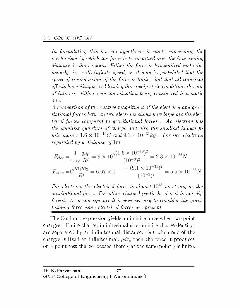
In formulating this law no hypothesis is made concerning themechanism by which the force is transmitted over the interveningdistance in the vacuum. Either the force is transmitted instanta-neously, ie., with in�nite speed, or it may be postulated that thespeed of transmission of the force is �nite , but that all transiente�ects have disappeared leaving the steady state condition, the oneof interest. Either way the situation being considered is a staticone.A comparison of the relative magnitudes of the electrical and grav-itational forces between two electrons shows how large are the elec-trical forces compared to gravitational forces . An electron hasthe smallest quantum of charge and also the smallest known �-nite mass : 1.6 × 10⁻¹⁹C and 9.1 × 10⁻³¹kg . For two electronsseparated by a distance of 1m
Felec =1
4πε0
qsqtR2
= 9× 10⁹ (1.6× 10⁻¹⁹)2
(10−3)2= 2.3× 10⁻²²N
Fgrav =Gm1m2
R2= 6.67× 1−−11 (9.1× 10⁻³¹)2
(10−3)2= 5.5× 10−65N
For electrons the electrical force is almost 1043 as strong as thegravitational force. For other charged particels also it is not dif-ferent. As a consequence,it is unnecessary to consider the gravi-tational force when electrical forces are present.
The Coulomb expression yields an in�nite force when two pointcharges ( Finite charge, in�nitesimal size, in�nite charge density)are separated by an in�nitesimal distance. But when one of thecharges is itself an in�nitesimal, ρdτs then the force it produceson a point test charge located there ( at the same point ) is �nite.
Dr.K.ParvatisamGVP College of Engineering ( Autonomous )
77

3.1. COULOMB'S LAW
3.1.3 PRINCIPLE OF SUPERPOSITION:
If there are more than two point charges the principle of superposition can be applied to determine the force on a particularcharge because of all the reaming charges. The principle statesthat if there are ′N ′ charges Q1, Q2, Q3 . . . QN located respec-tively at points whose position vectors are r1, r2, r3 . . . rN , theresultant force Fon charge Q located at a point whose positionvector is r is the vector sum of the forces exerted onQ by chargesQ1, Q2, Q3, . . . QN is
F =QQ1
4πε0
r − r1
|r − r1|3+QQ2
4πε0
r − r2
|r − r2|3+. . .+
QQN
4πε0
r − rN|r − rN |3
(3.9)
The above can also be expressed as a summation
F =Q
4πε0
N∑k=1
Qk(r − rk)|r − rk|3
(3.10)
If Q1 = Q2 = 1C and R12 = 1m the force acting between thesecharges is = 9× 10⁹ N. .An enormous force. The
electricalforcesare huge
The exponent in Coulomb's law di�ers from '2' by one part inone billion. Coulomb's law is valid for distances of the order of10−13cm. The law fails at distances of the order of 10−14cm. Itis also valid for distances of several kilo metes.
Example:
As an example consider a charge of 3×10⁻⁴C at P (1, 2, 3) anda charge of −10−4C at Q(2, 0, 5) in vacuum. Find the force actingon charge at Q .
Dr.K.ParvatisamGVP College of Engineering ( Autonomous )
78

3.1. COULOMB'S LAW
Ans:Q1 = 3× 10⁻⁴ and Q2 = −10−4
R12 = r2 − r1 = (2− 1)ax + (0− 2)ay + (5− 3)az (3.11)
= ax − 2ay + 2az (3.12)
a12 =ax − 2ay + 2az
3
F2 =3× 10⁻⁴(−10−4)
4π(
136π
)10−9
(ax − 2ay + 2az
3
)F2 = −30
(ax − 2ay + 2az
3
)N
Example:
Point charges 1mC and −2mC are located at (3, 2,−1) and(−1,−1, 4) respectively. Calculate the electrical force on a 10nCcharge located at (0, 3, 1) .
Ans:
F =2∑
k=1
QQk
4πε0
r − rk|r − rk|3
F = 10× 10−9 × 9× 109 × 10−3
((−3, 1, 2)
[(0, 3, 1)− (3, 2,−1)]3− 2(1, 4,−3)
[(0, 3, 1)− (−1,−1, 4)]3
)F = 9× 10⁻²
((−3, 1, 2)
14√
14+
(−2,−8, 6)
26√
26
)F = −6.507ax − 3.817ay + 7.506azmN
Dr.K.ParvatisamGVP College of Engineering ( Autonomous )
79

3.1. COULOMB'S LAW
Example:
2mC charge (positive) is located at P1(3,−2,−4) and a 5µCcharge (negative) is at P2(1,−4, 2)
1. Find the vector force on the negative charge
2. Also �nd the magnitude of the force
Ans:
R12 = [(1,−4, 2)− (3,−2,−4)] = −2ax − 2ay + 6az
|R12| =√
44 , aR12=−2ax − 2ay + 6az√
44
F12 = (2× 10⁻³)(−5× 10−6)× 9× 109
(−2ax − 2ay + 6az
44√
44
)F12 = 0.613ax + 0.613ay − 1.84az N
|F12| =√
(0.613)2 + (0.613)2 + (1.84)2 = 2.034 N
Example:
It is required to hold four equal point charges q C each inequilibrium at the corners of a square of side a meters. Provethat the point charge which can do this is a negative charge ofmagnitude
(2√
2 + 1)
4q (3.13)
coulombs placed at the center of the square.
Dr.K.ParvatisamGVP College of Engineering ( Autonomous )
80

3.2. ELECTRIC FIELD
3.2 ELECTRIC FIELD
Consider one charge �xed in position, sayQ1 with position vectorR1 and move a second charge slowly around, it can be seen thatthere exists everywhere a force on the second charge. In otherwords, the second charge is displaying the existence of a force�eld. If the test charge is denoted by Qt , the force on it is givenby Coulomb's law as
Ft =Q1Qt
4πε0R21t
aR1t(3.14)
Writing this force as a force per unit charge gives
FtQt
=Q1
4πε0R21t
aR1t(3.15)
The force is only a function of Q1 and is a directed segment fromQ1 to the position of the test charge. This is a vector �eld and iscalled the Electric Field intensity.
Electric �eld intensity can be de�ned as vector force on a unitpositive test charge. The units are Newton/Coulomb. Anticipat-ing a new quantity Volt which will be de�ned later, the unit forelectric �eld intensity is normally given by Volt/meter.
The test charge should be small such that it will not disturbthe original �eld of the charge distribution under consideration.So the electric �eld intensity denoted by E is de�ned as
limQt→0
FtQt
(3.16)
Electrical �eld of a point chargeLet the point charge be located at some point in a spherical co-
ordinate system at a distancer from the origin of the co-ordinate
Dr.K.ParvatisamGVP College of Engineering ( Autonomous )
81

3.2. ELECTRIC FIELD
system. 'E' can be expressed as
E =Q
4πε0r2ar (3.17)
In Cartesian co-ordinates r = xax + yay + zaz and
ar =xax + yay + zaz√
x2 + y2 + z2(3.18)
The �eld is spherically symmetric. If the charge is not at theorigin, the �eld will not be spherically symmetric. If the sourcecharge is at r′ = x′ax + y′ay + z′az, the �eld at a general pointr = xax + yay + zaz is given by
E =Q
4πε0 |r − r′|2r − r′|r − r′| (3.19)
3.2.1 ELECTRIC FIELD BECAUSE OF CHARGE DISTRI-BUTIONS:
Charge distributions can be of three types
1. Line charge distribution C/m
2. Surface charge distribution C/m2
3. Volume charge distribution C/m3 The total charge in a givencon�guration can be obtained as
dQ = ρLdl and Q =
ˆρLdl (3.20)
dQ = ρsds and Q =
ˆρsds (3.21)
Dr.K.ParvatisamGVP College of Engineering ( Autonomous )
82

3.2. ELECTRIC FIELD
dQ = ρvdv and Q =
ˆρvdv (3.22)
The electric �elds because of the distributions are given by
E =
ˆρLdl
4πε0R2aR (3.23)
E =
ˆρsds
4πε0R2aR
E =
ˆρvdv
4πR2aR
Figure 3.2: Charge Distributions
Dr.K.ParvatisamGVP College of Engineering ( Autonomous )
83

3.2. ELECTRIC FIELD
3.2.2 FIELD BECAUSE OF A FINITE LINE CHARGE:
Consider a line of �nite length with uniform charge density ρLC/m extending from A to b along the Z − axis as shown in the�gure.The charge in the element dl = dz is dQ and is given byρLdz. The total charge is given by
Q =
ˆ zB
zA
ρLdz (3.24)
The source point is (x, y, z), the �eld point is (x′, y′, z′), so dl =dz′
R = xax + yay + (z − z′)az (3.25)
R = ρaρ + (z − z′)az (3.26)
|R|2 = ρ2 + (z − z′)2 (3.27)aR
|R|3=
[ρaρ + (z − z′)az][ρ2 + (z − z′)2]
32
(3.28)
Then (3.29)
E =ρL
4πε0
ˆ[ρaρ + (z − z′)az][ρ2 + (z − z′)2]
32
(3.30)
De�ne α, α1 and α2 as shown in the �gure.
Dr.K.ParvatisamGVP College of Engineering ( Autonomous )
84

3.2. ELECTRIC FIELD
Figure 3.3: Line charge distribution
R = [ρ2 + (z − z′)2]12 = ρ secα (3.31)
z′ = oT − ρ tanα, dz′ = −ρ sec2 α dα (3.32)
E = − ρL4πε0
ˆ α2
α1
ρ secα [cosαaρ + sinαaz] dα
ρ2 sec2 α(3.33)
cosα =ρ
R, sinα =
(z − z′)R
(3.34)
Dr.K.ParvatisamGVP College of Engineering ( Autonomous )
85

3.2. ELECTRIC FIELD
E = − ρL4πε0
ˆ α2
α1
[cosαaρ + sinαaz] dα (3.35)
E =ρL
4πε0[(sinα1 − sinα2)aρ + (cosα2 − cosα1)az] (3.36)
3.2.3 CASE I: INFINITE LINE CHARGE:
For an in�nite line charge point B will be at (0, 0,∞) and pointA will be at (0, 0,−∞). so that α1 = π
2 , α2 = −π2 . Substitution
of the above values gives
E =ρL
2πε0ρaρ (3.37)
The z-component vanishes.
3.2.4 CASE II:LOWER END COINCIDINGWITH THE FIELDPOINT:
α1 = 0, α2 = tan−1 Lρ
E =ρL
4πε0ρ[(cosα2 − 1)az + sinα2aρ] (3.38)
Dr.K.ParvatisamGVP College of Engineering ( Autonomous )
86
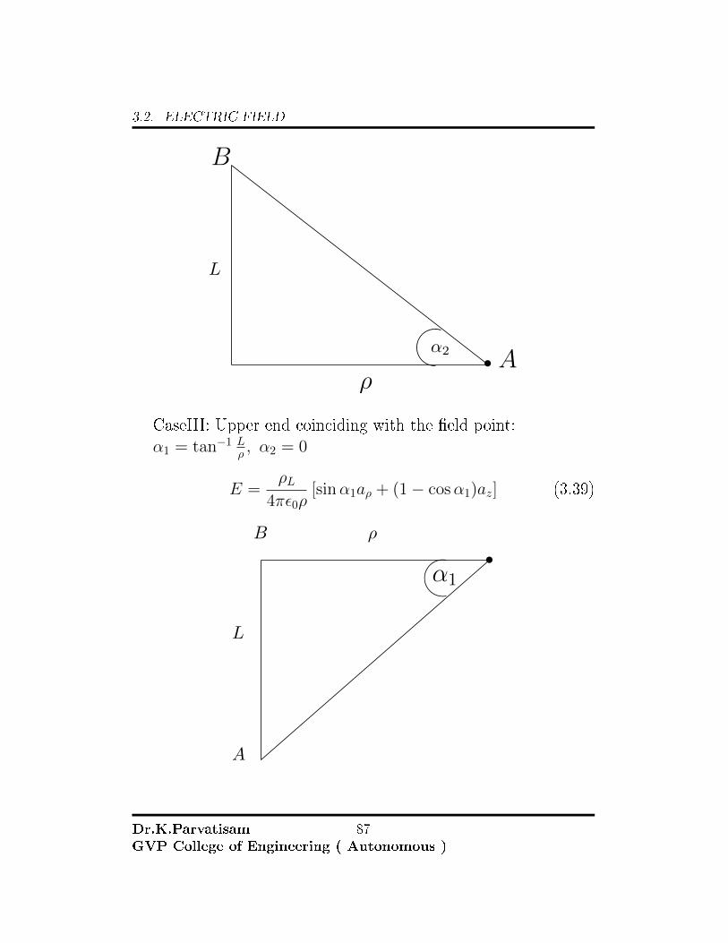
3.2. ELECTRIC FIELD
α2
ρ
L
A
B
CaseIII: Upper end coinciding with the �eld point:α1 = tan−1 L
ρ , α2 = 0
E =ρL
4πε0ρ[sinα1aρ + (1− cosα1)az] (3.39)
ρB
A
L
α1
Dr.K.ParvatisamGVP College of Engineering ( Autonomous )
87
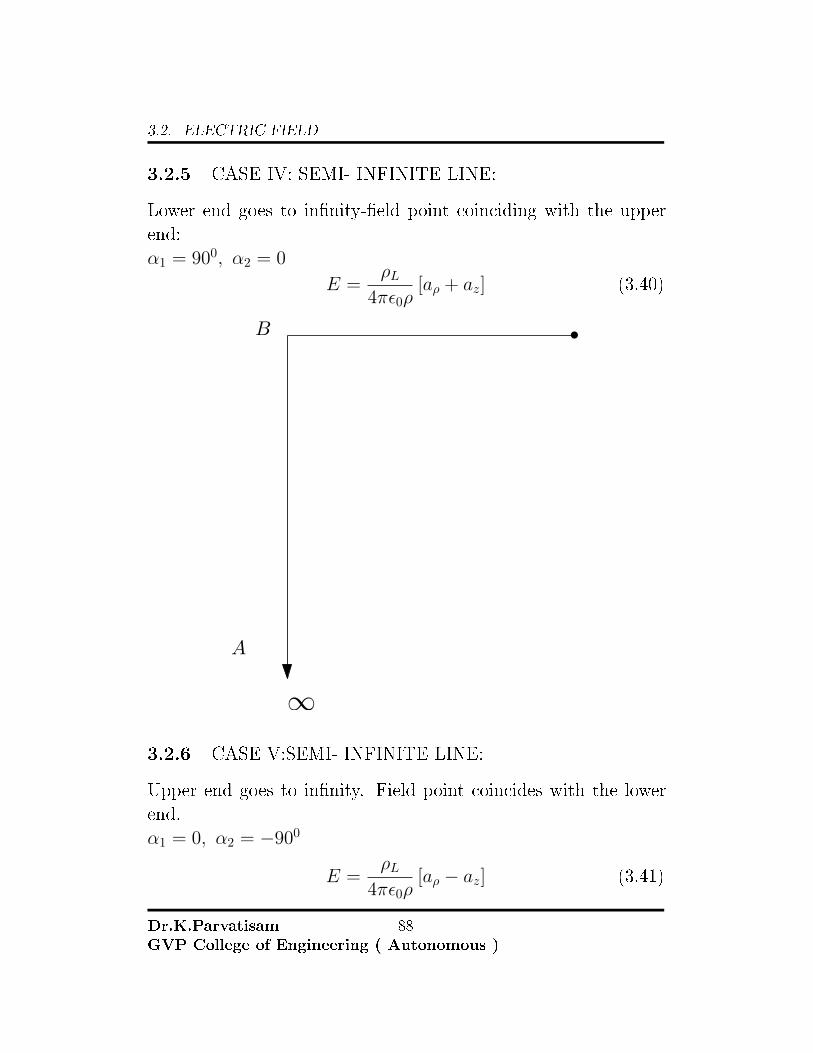
3.2. ELECTRIC FIELD
3.2.5 CASE IV: SEMI- INFINITE LINE:
Lower end goes to in�nity-�eld point coinciding with the upperend:α1 = 900, α2 = 0
E =ρL
4πε0ρ[aρ + az] (3.40)
B
A
∞3.2.6 CASE V:SEMI- INFINITE LINE:
Upper end goes to in�nity. Field point coincides with the lowerend.α1 = 0, α2 = −900
E =ρL
4πε0ρ[aρ − az] (3.41)
Dr.K.ParvatisamGVP College of Engineering ( Autonomous )
88

3.2. ELECTRIC FIELD
A
∞B
3.2.7 CASE VI: SEMI INFINITE LINE:
General point. Line extending from 0 to ∞ .α1 = α1, α2 = −900
E =ρL
4πε0ρ[(sinα1 − 1)aρ − cosα1az] (3.42)
Dr.K.ParvatisamGVP College of Engineering ( Autonomous )
89

3.2. ELECTRIC FIELD
∞B
A
0
Field Pointα1
900
3.2.8 CASE VII:SEMI-INFINITE LINE:
General point. Line extending from 0 , −∞α1 = 900, α2 = α2
E =ρL
4πε0ρ[(1 + sinα2)aρ + cosα2az] (3.43)
Dr.K.ParvatisamGVP College of Engineering ( Autonomous )
90

3.2. ELECTRIC FIELD
Field Point
∞
B
A
0
α2
900
3.2.9 CIRCULAR RING OF CHARGE:
To �nd the �eld at any point on the axis of a circular ring ofcharge, whose axis coincides with the z axis. The charge density isρLC/m. The radius of the ring is a m Consider a small di�erentiallength dl = adφ on the ring. Consider a point (0, 0, h) . Thdistance between the charge element and the point on the z axisis
Dr.K.ParvatisamGVP College of Engineering ( Autonomous )
91

3.2. ELECTRIC FIELD
Figure 3.4: Ring of charge
R = −aaρ + haz (3.44)
The total charge in the di�erential length element is dQ = ρLadφ
|R| = (a2 + h2)12 (3.45)
aR =R
|R|3=−aaρ + haz
(a2 + h2)32
(3.46)
E =ρL
4πε0
ˆ 2π
φ=0
(−aaρ + haz)
(a2 + h2)32
adφ (3.47)
Dr.K.ParvatisamGVP College of Engineering ( Autonomous )
92

3.2. ELECTRIC FIELD
The above is a sum of two integrals and the �rst one over 0 to 2πis equal to zero as aρ = cosφax− sinφay So the resulting integralis
E =ρL
4πε0
ah
(a2 + h2)32
az
ˆ 2π
0
dφ =ρL
4πε0
ah
(a2 + h2)32
az × 2π (3.48)
The result is
E =ρLah
2ε0(a2 + h2)32
az (3.49)
Maximum value of E:To �nd the maximum value of E equate dE
dh to zero. This givesh = ± a√
2As a → 0 the ring behaves like a point charge. If the
total charge on the ring is Q then ρL = Q2πa Then
E =Qh
4πε0[h2 + a2]32
az (3.50)
as a→ 0
E =Q
4πε0h2az (3.51)
Same as the �eld of a point charge.
3.2.10 SURFACE CHARGE DISTRIBUTION:
Assume a disk of radius ′a′m with a surface charge density ρsC/m2.Assumethat the axis coincides with the z − axis. It Is required to �ndthe �eld at any point (0, 0, h) on the axis of the disk. Consider asmall surface area element
Dr.K.ParvatisamGVP College of Engineering ( Autonomous )
93
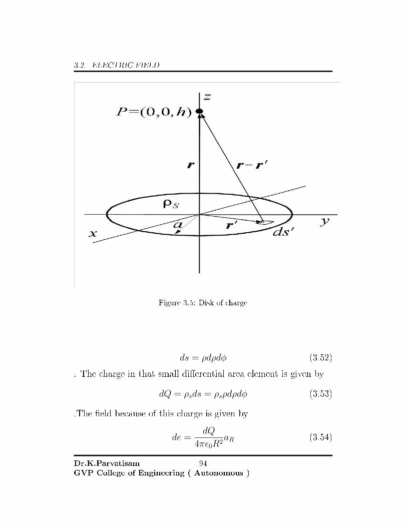
3.2. ELECTRIC FIELD
Figure 3.5: Disk of charge
ds = ρdρdφ (3.52)
. The charge in that small di�erential area element is given by
dQ = ρsds = ρsρdρdφ (3.53)
.The �eld because of this charge is given by
de =dQ
4πε0R2aR (3.54)
Dr.K.ParvatisamGVP College of Engineering ( Autonomous )
94

3.2. ELECTRIC FIELD
whereR = −ρaρ + haz (3.55)
and
aR =R
|R| =−ρaρ + haz√
ρ2 + h2(3.56)
Th e �eld because of the complete disk is
e =
ˆdE =
ˆ a
0
ˆ 2π
0
[ρsρdρdφ
4πε0
{−ρaρ + haz)
[ρ2 + h2]32
](3.57)
The �rst term containing the unit vector aρ is zero integrated over0 to2π. The second term that remains is
E =ρs
4πε0
ˆ a
0
ˆ 2π
0
hρdρdφ
[ρ2 + h2]32
az (3.58)
Integration by substitution of variable
ρ = h tan θ (3.59)
results in
E =ρs2ε0
{1− h
[h2 + a2]12
}az (3.60)
As a → ∞ the charge con�guration tends to an in�nite sheet ofcharge and the �eld is equal to
E =ρs2ε0
az (3.61)
that is, E has only z− component if the charge is in the x− yplane. In general, for an in�nite sheet of charge
E = ρs2ε0an
Dr.K.ParvatisamGVP College of Engineering ( Autonomous )
95

3.3. ENERGY AND POTENTIAL
where an is a unit vector normal to the sheet. From the aboveequation it can be noticed that the electric �eld is normal to thesheet and is independent of the distance between the sheet andthe point of observation P .
In a parallel plate capacitor, the electric �eld existing betweentwo plates having equal and opposite charges is given by
E =ρs2ε0
an +−ρs2ε0
(−an) =ρsε0an (3.62)
3.3 ENERGY AND POTENTIAL
3.3.1 ENERGY EXPENDED IN MOVING A POINT
CHARGE IN AN ELECTRIC FIELD:
Suppose we wish to move a charge Q a distance dL in an electric�eld E. The force on Q due to the electric �eld is
F = QE
where the subscript indicates that the force is due to the electric�eld. The component of this force in the direction of dL which anexternal force has to overcome is
FEL = F • aL = QE • aL (3.63)
where aL is a unit vector in the direction of dL The external forcethat must be applied is equal and opposite to the above force
Fappl = −QE • aL (3.64)
ordW = −QE • dL (3.65)
Dr.K.ParvatisamGVP College of Engineering ( Autonomous )
96

3.3. ENERGY AND POTENTIAL
The work done in moving a charge Q a �nite distance is deter-mined by integrating
W = −Qˆ final
initial
E • dL (3.66)
where the path must be speci�ed before the integration is per-formed.Th e charge is assumed to be at rest at both its initial and�nal positions.
Example: Given the electric �eldE = 1z2
(8xyzax + 4x2zay − 4x2yaz
)V/m.
Find the di�erential amount of work done in moving a 6 − nCcharge a distance 2µm, starting at P (2,−2, 3) and proceeding inthe direction aL =: i)− 6
7ax+ 37ay+
27az; ii)
67ax− 3
7ay− 27az; iii)
37ax+
67ay.
3.3.2 The LINE INTEGRAL:
The integral expression for the work done in moving a point chargeQ from one position to another, equation: is an example of a lineintegral. The procedure for evaluating the integral is shown in �g:, where a path has been chosen from an initial point B to a �nalpoint A and uniform electric �eld is selected for simplicity.
The path is divided into six segments ,4L1,4L2 . . .4L6
, and the components of E along each segment is denoted byEL1, EL2 . . . EL6
The involved in moving a charge Q from B to A is
w = −Q [EL14L1 + EL24L2 + . . . EL64L6] (3.67)
or using vector notation
w = −Q [EL1 • 4L1 + EL2 • 4L2 + . . . EL6 • 4L6] (3.68)
Dr.K.ParvatisamGVP College of Engineering ( Autonomous )
97

3.3. ENERGY AND POTENTIAL
as the �eld is uniform E1 = E2 = . . . E6
w = −QE • [4L1 +4L2 + . . .+4L6] (3.69)
The sum of all these small vector length segments is equal tothe vector directed from the initial point B to the �nal point A,and is denoted by LBA . Therefore
W = −QE • LBA (3.70)
This result for a uniform �eld can be written as an integral
W = −QA
B
E • dl (3.71)
Now we can de�ne potential di�erence V as the work done (by a nexternal agency) in moving a unit positive charge from one pointto another in an electric �eld
V =W
Q= −
finalˆ
initial
E • dl (3.72)
VAB signi�es the potential di�erence between points A and B
and is the work done in moving the unit positive charge from B
(last named) to A (the �rst named). In determining VAB , B isthe initial point and A is the �nal point. Potential di�erence ismeasured in Joules /Coulomb, which is commonly called as Volt.hence
VAB = −A
B
E•dL V
(3.73)
Dr.K.ParvatisamGVP College of Engineering ( Autonomous )
98

3.3. ENERGY AND POTENTIAL
and VAB is positive if work is done in carrying a positive chargefrom B to A .
3.3.2.1 THE POTENTIAL FIELD OF A POINT CHARGE:
To �nd the potential di�erence between pointsA and B at radialdistances rA and rB from a point chargeQ, assume that the originis at Q then
E = Erar =Q
4πε0r2ar (3.74)
anddL = drar (3.75)
we have
VAB = −A
B
E•dL = −rBˆ
rA
Q
4πε0r2dr =
Q
4πε0
(1
rA− 1
rB
)= VA−VB
(3.76)If rA > rB, the potential di�erence VAB is positive indicating
that energy is expended by external agent in bringing the positivecharge from rB to rA . See �gure below
Figure 3.6: Potential in the �eld of a point charge
Dr.K.ParvatisamGVP College of Engineering ( Autonomous )
99
3.3. ENERGY AND POTENTIAL
To speak of the potential or absolute potential, of a point,rather than the potential di�erence, an agreement must be reachedto measure the potential with respect to a speci�ed reference pointwhich should be considered to have zero potential. The most uni-versal zero reference point is �ground�. Theoretically it is rep-resented by an in�nite plane at zero potential. Another widelyused reference point is in�nity. This usually appears in theoret-ical problems. Also it is necessarily agreed that VA and VBshallhave the same zero reference point.
From the above �gure it can also be seen that the potentialdi�erence does not depend on path of integration, but dependsonly on the distance of each point from the charge( that is, onlyon the end points).
3.3.2.2 POTENTIAL FIELD BECAUSE OF AGROUP OF CHARGES:
The potential at a point has been de�ned as the work done inbringing a unit positive charge from the zero reference to the
point. Thus the potential of a single point chargeQ1 located atr1 at a point distant r from the origin with zero reference at
in�nity
V (r) =Q1
4πε0 |r − r1|(3.77)
The potential due to n charges is at this point is given by
V (r) =Q1
4πε0 |r − r1|+
Q2
4πε0 |r − r2|+ . . . . . .+
Qn
4πε0 |r − rn|(3.78)
Dr.K.ParvatisamGVP College of Engineering ( Autonomous )
100

3.3. ENERGY AND POTENTIAL
V (r) =n∑
m=1
Qm
4πε0 |r − rm|(3.79)
If each point charge is now represented as a small element of acontinuous volume charge distribution ρv4v, then
V (r) =
ˆ
vol
ρv(r′)dv′
4πε0 |r − r′|(3.80)
For line charge and also for surface charge distribution the respec-tive expressions are
V (r) =
ˆρL(r
′)dL′
4πε0 |r − r′|
V (r) =
ˆ
s
ρv(r′)ds′
4πε0 |r − r′|
3.3.2.3 THE POTENTIAL FIELD OF A RING OF UNIFORMLINE CHARGE DENSITY:
To �nd V on the axis of a uniform line charge ρL in the form aring of radius a , in the z = 0 plane as shown in �gure.
Dr.K.ParvatisamGVP College of Engineering ( Autonomous )
101

3.3. ENERGY AND POTENTIAL
Figure 3.7: Ring of charge
we have
dL′= adφ
′, r = zaz, r
′= aaρ,
∣∣∣r − r′∣∣∣ =√a2 + z2 (3.81)
and
V =
2πˆ
0
ρLadφ′
4πε0√a2 + z2
=ρLa
2ε0√a2 + z2
(3.82)
so potential at any point on the axis of a uniformly charged ringis
V = ρLa
2ε0√a2+z2
Dr.K.ParvatisamGVP College of Engineering ( Autonomous )
102

3.3. ENERGY AND POTENTIAL
3.3.2.4 POTENTIAL AT ANY POINT ON THE AXIS OF UNI-FORMLY CHARGED DISC:
dq = ρs2πrdr
dV =dq
4πε0R
R =√r2 + h2
dV =ρs2πrdr
4πε0√r2 + h2
V =ρs2ε0
aˆ
0
rdr√r2 + h2
V =ρs2ε0
h (secα− 1) + C
Dr.K.ParvatisamGVP College of Engineering ( Autonomous )
103

3.3. ENERGY AND POTENTIAL
If C = 0 at z =∞
V =ρs2ε0
h (secα− 1) (3.83)
Example:A charge of QC is distributed homogeneously over the surface
of a sphere of radius R meters. The sphere is in vacuum . Findthe potential V as a function of distance r from the center of thesphere for 0 ≤ r ≤ ∞ . V (∞) = 0.
Answer:Outside the sphere
V = −rˆ
∞
E • dr r > R
V = − Q
4πε0
rˆ
∞
dr
r2=
Q
4πε0r
Inside the sphere:
V (r) = −rˆ
∞
E•dr = − 1
4πε0
rˆ
∞
Q
r2dr −
R
r
(0)dr
=1
4πε0
Q
R(r < R)
(3.84)
Dr.K.ParvatisamGVP College of Engineering ( Autonomous )
104

3.3. ENERGY AND POTENTIAL
3.3.2.5 POTENTIAL AND ELECTRIC FIELD OF A DIPOLE:
An electric dipole is formed by two point charges of equal magni-tude and opposite sign (+Q,−Q) separated by a short distanced. The potential at the point P due to the electric dipole is foundusing superposition.
Dr.K.ParvatisamGVP College of Engineering ( Autonomous )
105

3.3. ENERGY AND POTENTIAL
Figure 3.8: Dipole
If the �eld point P is moved a large distance from the electricdipole (in what is called the far �eld, r � d the lines connectingthe two charges and the coordinate origin with the �eld pointbecome nearly parallel.
Dr.K.ParvatisamGVP College of Engineering ( Autonomous )
106

3.3. ENERGY AND POTENTIAL
Figure 3.9: Far �eld approximation
V ≈Q
4πε0
[1
r − d2 cos θ
− 1
r + d2 cos θ
]
V ≈Q
4πε0
[(r + d
2 cos θ)−(r − d
2 cos θ)(
r2 − d2
4 cos2 θ) ]
as r � d the far �eld is
V =Qd cos θ
4πε0r2(3.85)
The electric �eld produced by the electric dipole is found bytaking the gradient of the potential.
Dr.K.ParvatisamGVP College of Engineering ( Autonomous )
107

3.3. ENERGY AND POTENTIAL
V = −∇E = −[∂V
∂rar +
1
r
∂V
∂θaθ
]= − Qd
4πε0
[cos θ
∂
∂r
(1
r2
)ar +
1
r3
∂
∂θ(cos θ)aθ
]= − Qd
4πε0
[cos θ
(− 2
r3
)ar +
1
r3(− sin θ)aθ
]=
Qd
4πε0r3[2 cos θar + (sin θ)aθ]
If the vector dipole moment is de�ned as
P = pap = Qdap (3.86)
where ap points from +Q to−Q. The dipole potential and electric�eld may be written as
V =Qd cos θ
4πε0r2=P • ar4πε0r2
E =P
4πε0r3[2 cos θar + sin θaθ]
Note that the potential and electric �eld of the electric dipoledecay faster than those of a point charge. For an arbitrarily lo-cated, arbitrarily oriented dipole, the potential can be written as
Dr.K.ParvatisamGVP College of Engineering ( Autonomous )
108

3.3. ENERGY AND POTENTIAL
Figure 3.10: Arbitrarily placed dipole
3.3.3 ENERGY STORED IN AN ELECTROSTATIC
FIELD:
The amount of work necessary to assemble a group of point chargesequals the total energy (We) stored in the resulting electric �eld.
Example (3 point charges): Given a system of 3 point charges,we can determine the total energy stored in the electric �eld ofthese point charges by determining the work performed to assem-ble the charge distribution. We �rst de�ne Vmn as the absolutepotential at Pm due to point charge Qn.
Dr.K.ParvatisamGVP College of Engineering ( Autonomous )
109

3.3. ENERGY AND POTENTIAL
Figure 3.11: Energy to move point charges
1. Bring Q1 to P1(no energy required).
2. Bring Q2 to P2 (work = Q2V21).
3. Bring Q3 to P3 (work = Q3V31 +Q3V32)
The total work done We = 0 +Q2V21 +Q3V31 +Q3V32
If we reverse the order in which the charges are assembled, thetotal energy required is the same as before.
1. Bring Q3 to P3 (No energy required)
2. Bring Q2 to P2 (work=Q2V23)
3. Bring Q1to P1 ( work done = Q1V12 +Q1V13)
Dr.K.ParvatisamGVP College of Engineering ( Autonomous )
110

3.3. ENERGY AND POTENTIAL
Total work done We = 0 +Q2V23 +Q1V12 +Q1V13
Adding the above two equations
2We = Q1V12 +Q1V13 +Q2V21 +Q2V23 +Q3V31 +Q3V32 (3.87)
We =1
2[(Q1(V12 + V13) +Q2(V21 + V23) +Q3(V31 + V32)] =
1
2[Q1V1 +Q2V2 +Q2V3]
(3.88)where Vm is the total absolute potential at Pm a�ecting Qm.In general, for a system of N point charges, the total energy in
the electric �eld is given by
We =1
2
N∑k=1
QkVk (3.89)
For line, surface or volume charge distributions, the discretesum total energy formula above becomes a continuous sum (in-tegral) over the respective charge distribution. The point chargeterm is replaced by the appropriate di�erential element of chargefor a line, surface or volume distribution: ρLdL, ρsds or ρvdv. Theoverall potential acting on the point charge Qk due to the otherpoint charges (Vk) is replaced by the overall potential (v) actingon the di�erential element of charge due to the rest of the chargedistribution. The total energy expressions becomes
We =1
2
ˆ
L
ρLdL (Line Charge) (3.90)
We =1
2
ˆ
s
ρsds (Surface Charge) (3.91)
Dr.K.ParvatisamGVP College of Engineering ( Autonomous )
111

3.3. ENERGY AND POTENTIAL
We =1
2
ˆ
v
ρvdv (V olume Charge) (3.92)
If a volume charge distribution ρv of �nite dimension is enclosedby a spherical surface S0 of radius r0, the total energy associatedwith the charge distribution is given by
Figure 3.12: Distribution of volume charge
Dr.K.ParvatisamGVP College of Engineering ( Autonomous )
112

3.3. ENERGY AND POTENTIAL
We = limr0→∞
1
2
ˆ
v
ρvV dv
= limr0→∞
[1
2
ˆ(∇ •D)V dv
](3.93)
Using the following vector identity,
(∇ •D)V = ∇ • (V D)−D • ∇V (3.94)
the expression for the total energy can be written as
We = limr0→∞
1
2
ˆ
v
[∇ • (V D)]dv
− limr0→∞
1
2
ˆ
v
(D • ∇V )dv
(3.95)
If we apply the divergence theorem to the �rst integral, we �nd
We = limr0→∞
[1
2
‹V D • ds
]− lim
r0→∞
1
2
ˆ
v
(D • ∇V )dv
(3.96)
For each equivalent point charge (ρvdv) that makes up thevolume charge distribution, the potential contribution onS0 variesas r−1 and electric �ux density (and electric �eld) contributionvaries as r−2. Thus, the product of the potential and electric �uxdensity on the surface So varies as r−3. Since the integration overthe surface provides a multiplication factor of only r2, the surfaceintegral in the energy equation goes to zero on the surface S0 ofin�nite radius. This yields where the integration is applied overall space. The divergence term in the integrand can be written interms of the electric �eld as
E = −∇V (3.97)
Dr.K.ParvatisamGVP College of Engineering ( Autonomous )
113

3.3. ENERGY AND POTENTIAL
such that the total energy (J) in the electric �eld is
We =1
2
˚
v
D • Edv =1
2
˚
v
ε0(E • E)dv =1
2
˚
v
ε0E2dv
(3.98)This can also be expressed as
dWe
dv=
1
2ε0E
2 (3.99)
dWe
dv is called the energy density and is given in J/m3.
Dr.K.ParvatisamGVP College of Engineering ( Autonomous )
114

3.4. GAUSS'S LAW:
3.4 GAUSS'S LAW:
Johann Carl Friedrich Gauss: (30April 1777 � 23 February 1855) wasa German mathematician and physicalscientist who contributed signi�cantlyto many �elds, including number the-ory, statistics, analysis, di�erential ge-ometry, geodesy, geophysics, electro-statics, astronomy and optics.Sometimes referred to as the Princepsmathematicorum (Latin, "the Prince ofMathematicians" or "the foremost of mathematicians")and "greatest mathematician since antiquity", Gauss hada remarkable in�uence in many �elds of mathematics andscience and is ranked as one of history's most in�uen-tial mathematicians.He referred to mathematics as "thequeen of sciences".
3.4.1 ELECTRIC FLUX DENSITY:
Consider a set of concentric metallic spheres, the outer one consist-ing of two hemi-spheres which could be �rmly clamped together.
1. with the equipment dismantled, the inner sphere was givena known positive charge.
2. the hemispheres were then clamped together around the chargedsphere with about 2cm of dielectric material between them
3. The outer sphere was discharged by connecting it momentar-ily to ground
Dr.K.ParvatisamGVP College of Engineering ( Autonomous )
115

3.4. GAUSS'S LAW:
4. The outer sphere was separated carefully, using tools madeup of insulating material in order not to disturb the inducedcharge on each hemisphere, and the negative induced chargeon each hemisphere was measured. See �g. below
Figure 3.13: Faraday's experiment
It can be found that the total charge on the outer charge wasequal in magnitude to the original charge placed on the innersphere and this was true regardless of the dielectric material sep-arating the two spheres. There was some sort of a "displacement"from the inner sphere to the outer sphere which was independentof the medium, this as the displacement �ux density or electrical�ux. Electrical �ux is represented by ψ
Dr.K.ParvatisamGVP College of Engineering ( Autonomous )
116

3.4. GAUSS'S LAW:
ψ = Q
and the electrical �ux is measured in Coulombs. Electric �uxdensity is represented by the letter D because of the name thatwas given initially "Displacement �ux density". The electrical �uxdensity D is a vector and is a member of the �ux density classof vector �elds. The direction of D at a point is the direction ofthe �ux lines at that point, and the magnitude is given by thenumber of �ux lines crossing a surface normal to the lines divedby the surface area. Refer to the �g. below
Figure 3.14: The electric �ux in the region between a pair of charged con-centric spheres
.
The electric �ux density is in the radial direction and has avalue of
Dr.K.ParvatisamGVP College of Engineering ( Autonomous )
117
3.4. GAUSS'S LAW:
D|r=a =Q
4πa2ar
D|r=b =Q
4πb2ar
and at a radial distance of r, a ≤ r ≤ b
D =Q
4πr2ar (3.100)
If we compare this result with the equation for electric �eld inten-sity of a point charge in free space
E =Q
4πε0r2ar (3.101)
So in free space
D = ε0E
For a general charge distribution E and D are given by
E =
ˆ
v
ρvdv
4πε0R2aR
D =
ˆ
v
ρvdv
4πR2aR
The �g. below shows clearly what is the �ux passing throughan open surface.
Dr.K.ParvatisamGVP College of Engineering ( Autonomous )
118

3.4. GAUSS'S LAW:
Figure 3.15: Electric �ux through an open surface
3.4.2 GAUSS'S LAW:
From the above it can be seen that the electric �ux passing throughany imaginary spherical surface lying between the two conduct-ing spheres is equal to the charge enclosed within that imaginarysurface. This enclosed charge can be a charge that is distributedon the surface of the inner sphere, or it may be concentrated asa point charge at the center of the imaginary sphere. also as oneCoulomb of charge produces one coulomb of �ux, the inner con-
Dr.K.ParvatisamGVP College of Engineering ( Autonomous )
119

3.4. GAUSS'S LAW:
ductor might as well be a cube or a queer shaped metal piece andstill the total induced charge on the outer sphere would still bethe same. The �ux distribution will no longer be the same as theprevious symmetrical distribution, but it will be some unknowndistribution. If the outer hemisphere is replaced by a closed sur-face of any odd shape, still the result will be the same. The gen-eralization of this concept leads to the following statement whichis known as Gauss law:
The electrical �ux ψ passing through any closed surface
is equal to the total charge enclosed by that surface.
Gauss's law constitutes one of the fundamental laws of electro-magnetism.
3.4.2.1 GAUSS'S LAW AND MAXWELL'S EQUATION:
If the �ux emanating from a closed surface is ψ then
ψ = Qenc (3.102)
that is
ψ =
˛
s
dψ =
˛
s
D • ds = Q =
ˆ
v
ρvdv
˛
s
D • ds =
ˆ
v
ρvdv (3.103)
By applying divergence theorem to the �rst term in the aboveequation
Dr.K.ParvatisamGVP College of Engineering ( Autonomous )
120

3.4. GAUSS'S LAW:
˛
s
D • ds =
ˆ
v
(∇ •D)dv =
ˆ
v
ρvdv (3.104)
which gives
∇ •D = ρv (3.105)˛
s
D • ds =
ˆ
v
ρvdv (3.106)
which is the �rst of the four Maxwell's equations both in dif-ferential and integral form.
3.4.2.2 POTENTIAL GRADIENT:
The electric �eld at any general point is given by
E =Q
4πε0
−→r −−→r′|r − r′|3
(3.107)
Every expression for E whether it is because of a point charge orbecause of a general charge distribution contains the term
−→r −−→r′|r − r′|3
(3.108)
hence we want to �nd the curl of the above quantity and showhow E is related to V the potential. From vector calculus
Dr.K.ParvatisamGVP College of Engineering ( Autonomous )
121

3.4. GAUSS'S LAW:
∇×−→r −−→r′|r − r′|3
=1
|r − r′|3∇× (−→r −−→r ′) +
[∇ 1
|r − r′|3]× [−→r −−→r ′]
∇× (−→r −−→r ′) = 0
∇ 1∣∣∣−→r −−→r′ ∣∣∣ = −3−→r −−→r ′|r − r′|5
The above results together with the observation that the crossproduct of a vector with a parallel vector is zero, is su�cient toprove that
∇×−→r −−→r ′|r − r′|3
= 0 (3.109)
So this shows that the curl of the electric �eld is zero. Then fromvector calculus we know that if the curl of a vector is zero then thevector can be expressed as the gradient of a scalar point function.Also it can be seen that
E =Q
4πε0
−→r −−→r′|r − r′|3
= −∇′[Q
4πε0
1
|r − r′|
](3.110)
where
V =Q
4πε0
1
|r − r′| (3.111)
is the scalar potential. Hence E and V are related by
E = −∇V
3.4.2.3 Static Electric Field And The Curl:
It is seen that ˛E • dl = 0 (3.112)
Dr.K.ParvatisamGVP College of Engineering ( Autonomous )
122

3.4. GAUSS'S LAW:
andE = −∇V (3.113)
So if we apply the Stoke's theorem˛E • dl =
ˆ
s
(∇× E) • ds = 0 (3.114)
This is true for any ds , so
∇× E = 0 (3.115)
So the second of the Maxwell's equations, both in integral anddi�erential form, which describe the electric �eld is
˛E • dl = 0 (3.116)
∇× E = 0 (3.117)
The Maxwell's equations which describe the static electric �eldare given below
Dr.K.ParvatisamGVP College of Engineering ( Autonomous )
123
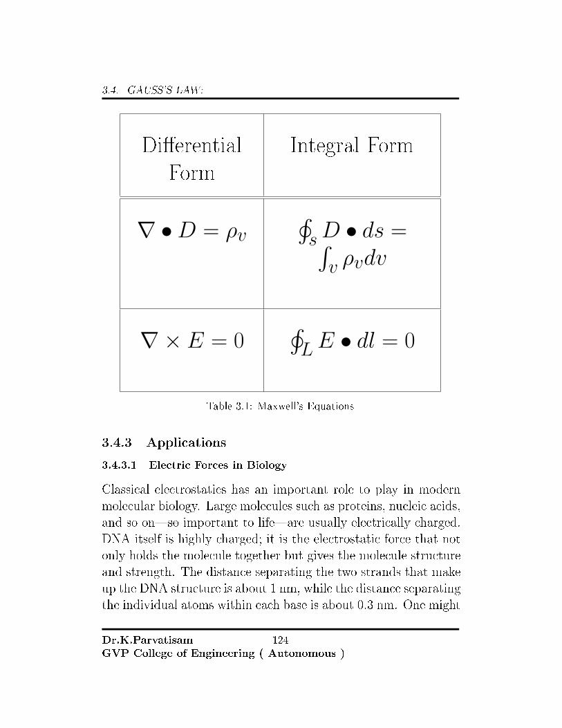
3.4. GAUSS'S LAW:
Di�erential
Form
Integral Form
∇ •D = ρv¸sD • ds =´v ρvdv
∇× E = 0¸LE • dl = 0
Table 3.1: Maxwell's Equations
3.4.3 Applications
3.4.3.1 Electric Forces in Biology
Classical electrostatics has an important role to play in modernmolecular biology. Large molecules such as proteins, nucleic acids,and so on�so important to life�are usually electrically charged.DNA itself is highly charged; it is the electrostatic force that notonly holds the molecule together but gives the molecule structureand strength. The distance separating the two strands that makeup the DNA structure is about 1 nm, while the distance separatingthe individual atoms within each base is about 0.3 nm. One might
Dr.K.ParvatisamGVP College of Engineering ( Autonomous )
124

3.4. GAUSS'S LAW:
wonder why electrostatic forces do not play a larger role in biologythan they do if we have so many charged molecules. The reason isthat the electrostatic force is �diluted� due to screening betweenmolecules. This is due to the presence of other charges in the cell.
3.4.3.2 Polarity of Water Molecules
The best example of this charge screening is the water molecule,represented as H2 O . Water is a strongly polar molecule. Its10 electrons (8 from the oxygen atom and 2 from the two hydro-gen atoms) tend to remain closer to the oxygen nucleus than thehydrogen nuclei. This creates two centers of equal and oppositecharges�what is called a dipole. The magnitude of the dipole iscalled the dipole moment. These two centers of charge will termi-nate some of the electric �eld lines coming from a free charge, ason a DNA molecule. This results in a reduction in the strength ofthe Coulomb interaction. One might say that screening makes theCoulomb force a short range force rather than long range. Otherions of importance in biology that can reduce or screen Coulombinteractions are Na+ , and K+ , and Cl− . These ions are locatedboth inside and outside of living cells. The movement of these ionsthrough cell membranes is crucial to the motion of nerve impulsesthrough nerve axons. Recent studies of electrostatics in biologyseem to show that electric �elds in cells can be extended over largerdistances, in spite of screening, by �microtubules� within the cell.These microtubules are hollow tubes composed of proteins thatguide the movement of chromosomes when cells divide, the mo-tion of other organisms within the cell, and provide mechanismsfor motion of some cells (as motors).
Dr.K.ParvatisamGVP College of Engineering ( Autonomous )
125

3.4. GAUSS'S LAW:
3.4.3.3 Earth's Electric Field
A near uniform electric �eld of approximately 150N/C, directeddownward, surrounds Earth, with the magnitude increasing slightlyas we get closer to the surface. What causes the electric �eld? Ataround 100 km above the surface of Earth we have a layer ofcharged particles, called the ionosphere. The ionosphere is re-sponsible for a range of phenomena including the electric �eldsurrounding Earth. In fair weather the ionosphere is positive andthe Earth largely negative, maintaining the electric �eld. In stormconditions clouds form and localized electric �elds can be largerand reversed in direction (Figure 18.34(b)). The exact chargedistributions depend on the local conditions, and variations arepossible. If the electric �eld is su�ciently large, the insulatingproperties of the surrounding material break down and it becomesconducting. For air this occurs at around 3×10⁶N/C. Air ionizesions and electrons recombine, and we get discharge in the form oflightning sparks and corona discharge.
Dr.K.ParvatisamGVP College of Engineering ( Autonomous )
126

3.4. GAUSS'S LAW:
Lightning
3.4.3.4 Applications of Conductors
On a very sharply curved surface, such as shown in Figure , thecharges are so concentrated at the point that the resulting elec-tric �eld can be great enough to remove them from the surface.This can be useful. Lightning rods work best when they are mostpointed. The large charges created in storm clouds induce anopposite charge on a building that can result in a lightning bolthitting the building. The induced charge is bled away continuallyby a lightning rod, preventing the more dramatic lightning strike.Of course, we sometimes wish to prevent the transfer of chargerather than to facilitate it. In that case, the conductor should
Dr.K.ParvatisamGVP College of Engineering ( Autonomous )
127

3.4. GAUSS'S LAW:
be very smooth and have as large a radius of curvature as possi-ble. (See Figure 18.37.) Smooth surfaces are used on high-voltagetransmission lines, for example, to avoid leakage of charge into theair. Another device that makes use of some of these principles isa Faraday cage. This is a metal shield that encloses a volume. Allelectrical charges will reside on the outside surface of this shield,and there will be no electrical �eld inside. A Faraday cage is usedto prohibit stray electrical �elds in the environment from inter-fering with sensitive measurements, such as the electrical signalsinside a nerve cell. During electrical storms if you are driving acar, it is best to stay inside the car as its metal body acts as aFaraday cage with zero electrical �eld inside. If in the vicinity ofa lightning strike, its e�ect is felt on the outside of the car and theinside is una�ected, provided you remain totally inside. This isalso true if an active (�hot�) electrical wire was broken (in a stormor an accident) and fell on your car.
Dr.K.ParvatisamGVP College of Engineering ( Autonomous )
128

3.4. GAUSS'S LAW:
A Sharp Conductor and its Electric �eld
3.4.3.5 The Van de Graa� Generator
Van de Graa� generators (or Van de Graa�s) are not only spectac-ular devices used to demonstrate high voltage due to static elec-tricity�they are also used for serious research. The �rst was builtby Robert Van de Graa� in 1931 (based on original suggestionsby Lord Kelvin) for use in nuclear physics research. Figure showsa schematic of a large research version. Van de Graa�s utilizeboth smooth and pointed surfaces, and conductors and insulatorsto generate large static charges and, hence, large voltages. A verylarge excess charge can be deposited on the sphere, because it
Dr.K.ParvatisamGVP College of Engineering ( Autonomous )
129

3.4. GAUSS'S LAW:
moves quickly to the outer surface. Practical limits arise becausethe large electric �elds polarize and eventually ionize surroundingmaterials, creating free charges that neutralize excess charge orallow it to escape. Nevertheless, voltages of 15 million volts arewell within practical limits.
Van de Grafe generator
3.4.3.6 Xerography
Most copy machines use an electrostatic process called xerog-raphy�a word coined from the Greek words xeros for dry andgraphos for writing. The heart of the process is shown in simpli-�ed form in Figure . A selenium-coated aluminum drum is sprayed
Dr.K.ParvatisamGVP College of Engineering ( Autonomous )
130
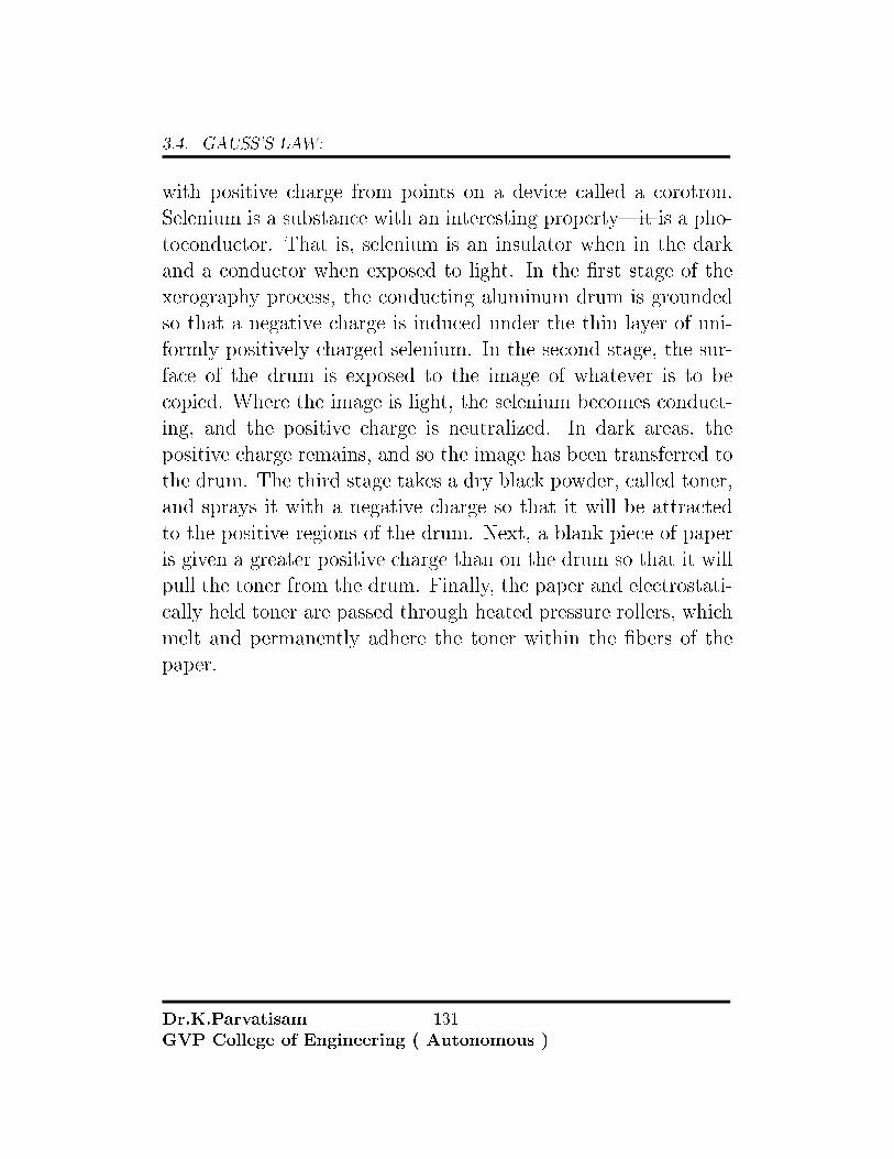
3.4. GAUSS'S LAW:
with positive charge from points on a device called a corotron.Selenium is a substance with an interesting property�it is a pho-toconductor. That is, selenium is an insulator when in the darkand a conductor when exposed to light. In the �rst stage of thexerography process, the conducting aluminum drum is groundedso that a negative charge is induced under the thin layer of uni-formly positively charged selenium. In the second stage, the sur-face of the drum is exposed to the image of whatever is to becopied. Where the image is light, the selenium becomes conduct-ing, and the positive charge is neutralized. In dark areas, thepositive charge remains, and so the image has been transferred tothe drum. The third stage takes a dry black powder, called toner,and sprays it with a negative charge so that it will be attractedto the positive regions of the drum. Next, a blank piece of paperis given a greater positive charge than on the drum so that it willpull the toner from the drum. Finally, the paper and electrostati-cally held toner are passed through heated pressure rollers, whichmelt and permanently adhere the toner within the �bers of thepaper.
Dr.K.ParvatisamGVP College of Engineering ( Autonomous )
131

3.4. GAUSS'S LAW:
3.4.3.7 Laser Printers
Laser printers use the xerographic process to make high-qualityimages on paper, employing a laser to produce an image on thephotoconducting drum as shown in Figure . In its most commonapplication, the laser printer receives output from a computer,and it can achieve high-quality output because of the precisionwith which laser light can be controlled. Many laser printers dosigni�cant information processing, such as making sophisticatedletters or fonts, and may contain a computer more powerful thanthe one giving them the raw data to be printed.
Dr.K.ParvatisamGVP College of Engineering ( Autonomous )
132
3.4. GAUSS'S LAW:
3.4.3.8 Ink Jet Printers and Electrostatic Painting
The ink jet printer, commonly used to print computer-generatedtext and graphics, also employs electrostatics. A nozzle makes a�ne spray of tiny ink droplets, which are then given an electrostaticcharge. Once charged, the droplets can be directed, using pairsof charged plates, with great precision to form letters and imageson paper. Ink jet printers can produce color images by using ablack jet and three other jets with primary colors, usually cyan,magenta, and yellow, much as a color television produces color.(This is more di�cult with xerography, requiring multiple drumsand toners.)
Dr.K.ParvatisamGVP College of Engineering ( Autonomous )
133

3.4. GAUSS'S LAW:
Ink jet Printer
3.4.3.9 Smoke Precipitators and Electrostatic Air Cleaning
Another important application of electrostatics is found in aircleaners, both large and small. The electrostatic part of the pro-cess places excess (usually positive) charge on smoke, dust, pollen,and other particles in the air and then passes the air through anoppositely charged grid that attracts and retains the charged par-ticles. Large electrostatic precipitators are used industrially toremove over 99% of the particles from stack gas emissions associ-ated with the burning of coal and oil. Home precipitators, often inconjunction with the home heating and air conditioning system,are very e�ective in removing polluting particles, irritants, andallergens.
Dr.K.ParvatisamGVP College of Engineering ( Autonomous )
134

3.4. GAUSS'S LAW:
Electrostatic Precipitators
Dr.K.ParvatisamGVP College of Engineering ( Autonomous )
135

Unit-II
Conductors And Dipole:
Laplace's and Poison's equations � Solution of Laplace's equa-tion in one variable. Electric dipole � Dipole moment � potentialand EFI due to an electric dipole � Torque on an Electric dipolein an electric �eld � Behavior of conductors in an electric �eld �Conductors and Insulators.

Chapter 4
POISSON'S AND LAPLACE'S
EQUATIONS:
Pierre-Simon, marquis de Laplace(23 March
1749 � 5 March 1827) was a French mathematicianand astronomer whose work was pivotal to the devel-opment of mathematical astronomy and statistics. Hesummarized and extended the work of his predecessors inhis �ve-volume Mécanique Céleste (Celestial Mechanics)(1799�1825). This work translated the geometric study ofclassical mechanics to one based on calculus, opening upa broader range of problems. In statistics, the so-calledBayesian interpretation of probability was mainly developed by Laplace.[1] Laplaceformulated Laplace's equation, and pioneered the Laplace transform which appearsin many branches of mathematical physics, a �eld that he took a leading role informing.The Laplacian di�erential operator, widely used in mathematics, is alsonamed after him. He restated and developed the nebular hypothesis of the origin ofthe solar system and was one of the �rst scientists to postulate the existence of blackholes and the notion of gravitational collapse. Laplace is remembered as one of thegreatest scientists of all time. Sometimes referred to as the French Newton or New-ton of France, he possessed a phenomenal natural mathematical faculty superior tothat of any of his contemporaries.[2] Laplace became a count of the First FrenchEmpire in 1806 and was named a marquis in 1817, after the Bourbon Restoration.
137

4.1. DERIVATION OF LAPLACE'S AND POISSON'S EQUATIONS:
Siméon Denis Poisson (21 June
1781 � 25 April 1840), was aFrench mathematician, geometer,and physicist. He obtained manyimportant results, but within theelite Académie des Sciences he alsowas the �nal leading opponent ofthe wave theory of light and was proven wrong on that matterby Augustin-Jean Fresnel.
4.1 DERIVATION OF LAPLACE'S AND POIS-
SON'S EQUATIONS:
The Poisson's equation can be derived from the point form ofGauss's law
∇ •D = ρv
D = εE
E = −∇V∇ •D = ∇ • (εE) = −∇ • (ε∇V ) = ρv
∇ •∇V = −ρvε
In the above equation ε is a constant.The equation is known as the Poisson's equation a and in Carte-
sian coordinates it is given as
∇ •∇V =∂2V
∂x2+∂2V
∂y2+∂2V
∂z2(4.1)
Dr.K.ParvatisamGVP College of Engineering ( Autonomous )
138

4.1. DERIVATION OF LAPLACE'S AND POISSON'S EQUATIONS:
The operation ∇ •∇ is abbreviated as ∇2 and we have
∇2V =∂2V
∂x2+∂2V
∂y2+∂2V
∂z2(4.2)
in cartesian coordinates.If ρv = 0 , indicating zero volume charge density , but allowing
point charges, line charges, and surface charge density to exist atsingular locations as sources of the �eld, then
∇2V = 0 (4.3)
which is Laplace's equation. The∇2 operation is called the Lapla-cian of V . In cartesian coordinates
∇2V =∂2V
∂x2+∂2V
∂y2+∂2V
∂z2(4.4)
In cylindrical coordinates
∇2V =1
ρ
∂
∂ρ
(ρ∂V
∂ρ
)+
1
ρ2
(∂2V
∂φ2
)+∂2V
∂z2(4.5)
In spherical coordinates
∇2V =1
r2
∂
∂r
(r2∂V
∂r
)+
1
r2 sin θ
∂
∂θ
(sin θ
∂V
∂θ
)+
1
r2 sin2 θ
∂2V
∂φ2
(4.6)Laplace's equation is all embracing , for, applying as it does wherevolume charge density is zero, it states that every conceivablecon�guration of electrodes or conductors produces a �eld for which∇2V = 0. All these �elds are di�erent , with di�erent potentialvalues and di�erent spatial rates of change, yet for each of them∇2V = 0 . Since every �eld ( if ρv = 0 ) satis�es Laplace,s
Dr.K.ParvatisamGVP College of Engineering ( Autonomous )
139
4.1. DERIVATION OF LAPLACE'S AND POISSON'S EQUATIONS:
equation , how can we expect to reverse the procedure and useLaplace's equation to �nd one speci�c �eld in which we happento to have an interest? Obviously more information is required,and we shall �nd that we must solve Laplace's equation subjectto certain boundary conditions.
Every physical problem must contain at least one conductingboundary and usually contains two or more . The potentials onthese boundaries are assigned values, perhaps V0, V1, · · · or per-haps numerical values. These de�nite equipotential surfaces willprovide the boundary conditions for the type of problem to besolved . In other types of problems , the boundary conditionstake the form of speci�ed values ofE on an enclosing surface, or amixture of known values of V and E . It is necessary to show thatif our answer satis�es the Laplace's equation and also satis�es theboundary conditions, then it is the only possible answer.
4.1.1 UNIQUENESS THEOREM:
Let us assume that we have two solutions of Laplace's equation,V1
and V2 , both general functions of the coordinates used. Therefore
∇2V1 = 0 (4.7)
and∇2V2 = 0 (4.8)
from which∇2(V1 − V2) = 0 (4.9)
Each solution must also satisfy the boundary conditions , and ifwe represent the given potential values on the boundaries by Vb ,then the value of V1 on the boundary V1b and the value of V2 on
Dr.K.ParvatisamGVP College of Engineering ( Autonomous )
140
4.1. DERIVATION OF LAPLACE'S AND POISSON'S EQUATIONS:
the boundary V2b must both be identical to Vb
V1b = V2b = Vb (4.10)
orV1b − V2b = 0 (4.11)
Using the vector identity which will hold for for any scalar V andvector D
∇ • (V D) = V (∇ •D) +D • (∇V ) (4.12)
For the present we will assume that V = V1−V2 is the scalar and∇(V1 − V2) as the vector, giving
∇•[(V1 − V2)∇ (V1 − V2)] = (V1 − V2) [∇ •∇ (V! − V2)]+∇ (V! − V2)•∇ (V1 − V2)(4.13)
which we will integrate throughout the volume enclosed by thebounding surfaces speci�edˆ
vol
∇•[(V1 − V2)∇ (V1 − V2)] dv =
ˆ
vol
(V1 − V2) [∇ •∇ (V! − V2)]+∇ (V! − V2)•∇ (V1 − V2) dv
(4.14)The divergence theorem allows us to replace the volume integralon the left side of the equation by the closed surface integral overthe surface surrounding the volume. this surface consists of theboundaries already speci�ed on which V1b = V2b , and thereforeˆ
vol
∇•[(V1 − V2)∇ (V1 − V2)] dv =
˛
s
[(V1b − V2b)∇ (V1b − V2b)]•ds = 0
(4.15)One of the factors of the �rst integral on the right side is∇•∇(V1−V2)or ∇2(V1−V2) which is zero by hypothesis , and therefore thatintegral is zero. Hence the volume integral must be zero.ˆ
vol
[∇ (V1 − V2)]2 dv = 0 (4.16)
Dr.K.ParvatisamGVP College of Engineering ( Autonomous )
141

4.1. DERIVATION OF LAPLACE'S AND POISSON'S EQUATIONS:
There are in general two reasons why an integral may be zero:either the integrand ( the quantity under the integral sign ) is ev-erywhere zero, or the integrand is positive in regions and negativein others, and the contributions cancel algebraically. In this casethe �rst reason must hold good because [∇(V1− V2)]
2 can not benegative. Therefore
[∇ (V1 − V2)]2 = 0 (4.17)
and∇(V1 − V2) = 0 (4.18)
Finally, if the gradient of V1−V2 is everywhere zero , then V1−V2
can not change with any coordinates and
V! − V2 = Constant (4.19)
If we can show that t5his constant is zero, we shall have accom-plished our proof . The constant is easily evaluated by consideringa point on the boundary . Here V1 − V2 = V1b − V2b = 0 , and wesee that the constant is indeed zero, and therefore
V1 = V2 (4.20)
giving two identical solutions.The uniqueness theorem also is applicable to Poisson's equa-
tion, for if ∇2V1 = −ρvε and ∇2V2 = −ρv
ε , then , ∇2(V1−V2) = 0as before. Boundary conditions still require that V1b − V2b = 0 ,and the proof is identical from this point.
4.1.2 EXAMPLES:
Several methods have been developed for solving the second orderpartial di�erential equation known as Laplace's equation . The
Dr.K.ParvatisamGVP College of Engineering ( Autonomous )
142

4.1. DERIVATION OF LAPLACE'S AND POISSON'S EQUATIONS:
�rst and simplest method is that of direct integration, and we shalluse this technique to work several examples in various coordinatesystems.
The method of direct integration is applicable only to problemswhich are one dimensional or in which the potential �eld is a func-tion of only one of the three coordinates. Since we are workingwith only three coordinate systems, it might seem that there arenine problems to be solved, but a little re�ection will show that a�eld which varies only with x is fundamentally the same as withy.Rotating the physical problem a quarter turn is no change. Ac-tually, there are only �ve problems to be solved , one in cartesiancoordinates, two in cylindrical coordinates, and two in sphericalcoordinates.
Example:let us assume that V is a function only of x and worry later
about which physical problem we are solving when we have aneed for boundary conditions. Laplace's equation reduces to
∂2V
∂x2= 0 (4.21)
and the partial derivative may be replaced by an ordinaryderivative , since V is not a function of y or z ,
d2V
dx2= 0 (4.22)
we integrate twice , obtaining
dV
dx= A , V = Ax+B (4.23)
where A and B are constants of integration. These constants canbe determined only from the boundary conditions. Since the �eld
Dr.K.ParvatisamGVP College of Engineering ( Autonomous )
143

4.1. DERIVATION OF LAPLACE'S AND POISSON'S EQUATIONS:
varies only with x and is not a function of yand z , then V isa constant if x is a constant or in other words, the equipotentialsurfaces are described by setting x constant. These surfaces areparallel planes normal to the xaxis. the �eld is thus of a parallelplate capacitor,and as soon as we specify the potential on any twoplanes , we may evaluate our constants of integration.
Let V = V1 at x = x1and V = V2 at x = x2 . These values arethen substituted giving
V1 = Ax1 +B
V2 = Ax2 +B
A =V! − V2
x1 − x2B =
V2x1 − V1x2
x1 − x2
V =V1(x− x2)− V2(x− x1)
x1 − x2(4.24)
The general solution is
V = mx+ b (4.25)
a straight line equation. If V = 4 at x = 1 and V = 0 at x = 5 ,then m = −1 and b = 5 . Then
V = −x+ 5 (4.26)
The above solution has two properties
1. V (x) is the average of V (x+R) and V (x−R)
V (x) =1
2[V (x+R) + V (x−R)] (4.27)
Laplace's equation is a kind of averaging instruction. It tellsyou to assign to the point x , the average of the value to theleft and to the right of x .
Dr.K.ParvatisamGVP College of Engineering ( Autonomous )
144

4.1. DERIVATION OF LAPLACE'S AND POISSON'S EQUATIONS:
Figure 4.1: Graph Of V = −x+ 5
2. Laplace's equation tolerates no local maxima . Extreme val-ues of V must occur at the end points . This is a consequenceof property 1 .
A simple answer would have been obtained by choosing simplerboundary conditions. If we had �xed V = 0 at x = 0 and V =V0 at x = d , then
A =V0
dB = 0
and
V =V0x
d(4.28)
Suppose our primary aim is to �nd the capacitance of a parallelplate capacitor. We have solved Laplace's equation , obtaining thetwo constants A and B . We are not interested in the potential�eld itself , but only in the capacitance, then we may continue
Dr.K.ParvatisamGVP College of Engineering ( Autonomous )
145

4.1. DERIVATION OF LAPLACE'S AND POISSON'S EQUATIONS:
successfully with A and b or we may simplify the algebra by littleforesight. Capacitance is given by the ratio of charge to potentialdi�erence , so we may chose now the potential di�erence as V0 ,which is equivalent to one boundary condition, and then choosewhatever second boundary condition seems to help the form of theequation the most. This is what we did while choosing the secondset of boundary conditions. The potential di�erence is �xed asV0 by choosing the potential of plate zero and the other V0; thelocation of these plates was made as simple as possible by lettingV = 0 at x = 0.
We still need the total charge on either plate before the capac-itance can be found. The necessary steps are these
1. Given V , use E = −∇V to �nd E
2. Use D = εE to �nd D
3. Evaluate D at either of the plates , D = Ds = DNaN
4. Recognize that ρs = DN
5. Find Q by surface integration over the capacitor plate ,Q =´s ρsds
Here we have
Dr.K.ParvatisamGVP College of Engineering ( Autonomous )
146

4.2. ELECTRIC DIPOLE
V = V0x
d
E = −V0
dax
D = −εV0
dax
Ds = D|x=0 = −εV0
dax
aN = ax
DN = −εV0
d= ρs
Q =
ˆ
s
−εV0
dds = −εV0S
d
and the capacitance is
C =|Q|V0
=εS
d(4.29)
4.2 Electric Dipole
4.2.1 POTENTIAL AND ELECTRIC FIELD OF ADIPOLE:
An electric dipole is formed by two point charges of equal magni-tude and opposite sign (+Q,−Q) separated by a short distanced. The potential at the point P due to the electric dipole is foundusing superposition.
Dr.K.ParvatisamGVP College of Engineering ( Autonomous )
147
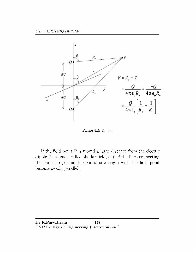
4.2. ELECTRIC DIPOLE
Figure 4.2: Dipole
If the �eld point P is moved a large distance from the electricdipole (in what is called the far �eld, r � d the lines connectingthe two charges and the coordinate origin with the �eld pointbecome nearly parallel.
Dr.K.ParvatisamGVP College of Engineering ( Autonomous )
148
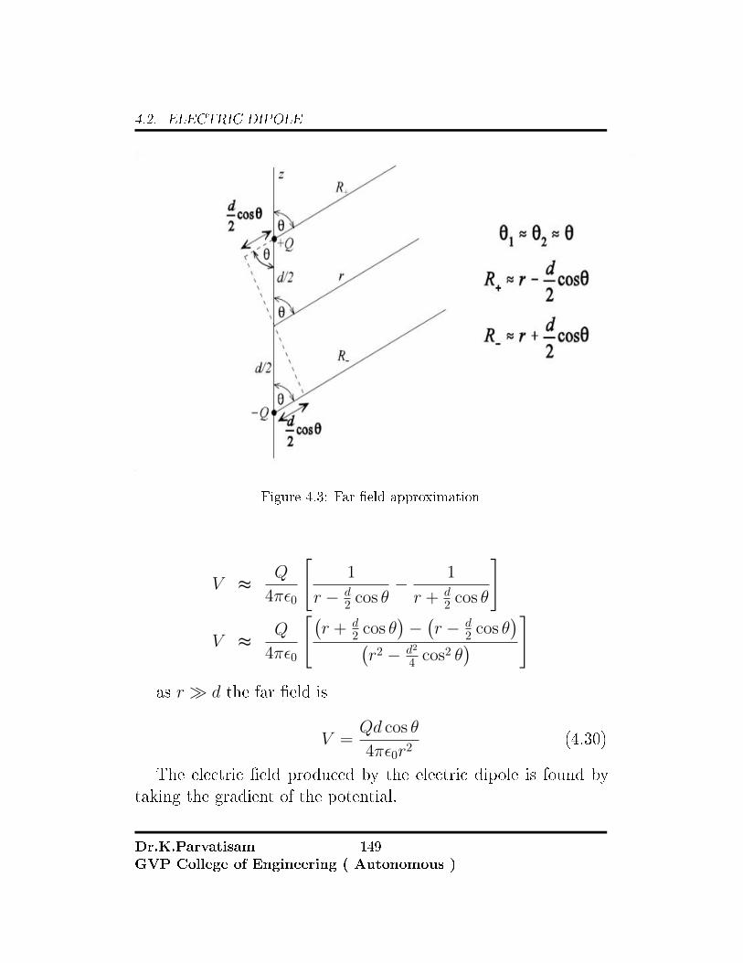
4.2. ELECTRIC DIPOLE
Figure 4.3: Far �eld approximation
V ≈Q
4πε0
[1
r − d2 cos θ
− 1
r + d2 cos θ
]
V ≈Q
4πε0
[(r + d
2 cos θ)−(r − d
2 cos θ)(
r2 − d2
4 cos2 θ) ]
as r � d the far �eld is
V =Qd cos θ
4πε0r2(4.30)
The electric �eld produced by the electric dipole is found bytaking the gradient of the potential.
Dr.K.ParvatisamGVP College of Engineering ( Autonomous )
149

4.2. ELECTRIC DIPOLE
V = −∇E = −[∂V
∂rar +
1
r
∂V
∂θaθ
]= − Qd
4πε0
[cos θ
∂
∂r
(1
r2
)ar +
1
r3
∂
∂θ(cos θ)aθ
]= − Qd
4πε0
[cos θ
(− 2
r3
)ar +
1
r3(− sin θ)aθ
]=
Qd
4πε0r3[2 cos θar + (sin θ)aθ]
If the vector dipole moment is de�ned as
P = pap = Qdap (4.31)
where ap points from +Q to−Q. The dipole potential and electric�eld may be written as
V =Qd cos θ
4πε0r2=P • ar4πε0r2
E =P
4πε0r3[2 cos θar + sin θaθ]
Note that the potential and electric �eld of the electric dipoledecay faster than those of a point charge. For an arbitrarily lo-cated, arbitrarily oriented dipole, the potential can be written as
Dr.K.ParvatisamGVP College of Engineering ( Autonomous )
150

4.2. ELECTRIC DIPOLE
Figure 4.4: Arbitrarily placed dipole
V =P •
(r−r′|r−r′|
)4πε0 |r − r′|2
=P • (r − r′)4πε0 |r − r′|3
|r − r′| >>d
Dr.K.ParvatisamGVP College of Engineering ( Autonomous )
151

4.2. ELECTRIC DIPOLE
4.2.2 Torque On A Dipole In an Electric Field
d
+Q
−Ql
θ
F1
F2
The dipole moment is given by
p = Qd (4.32)
It is a vector directed from the negative to positive charge formingthe dipole. The potential at any point because of the dipole isgiven by
V =p • ar4πε0r2
(4.33)
What happens when a dipole is placed in a uniform electric �eld?Will it experience a force ? There are two charges Q and −Qforming the dipole, each of which experiences a force equal inmagnitude to QE but oppositely directed, with the result thatthe dipole experiences no tanslational force , as forces F1 and F2
neutralize is other, but these forces form a couple, whose torqueis equal in magnitude to force X length of the arm of the couple.
T = (QE) l = QEd sin θ
T = Qd (E sin θ)
T = pE sin θ
T = p× E
Dr.K.ParvatisamGVP College of Engineering ( Autonomous )
152

4.2. ELECTRIC DIPOLE
Although a dipole in a uniform �eld does not experience a trans-lational force , it does experience a torque tending to align thedipole axis with the �eld direction.
4.2.3 Conductors, Semiconductors, and Insulators
Electrons surrounding the positive atomic nucleus are describedin terms of the total energy of the electron with respect to a zeroreference level for an electron at an in�nite distance from thenucleus. The total energy is the sum of the kinetic and potentialenergies , and since energy must be given to an electron to pull itaway from the nucleus, the energy of every electron in the atomis a negative quantity. It is convenient to associate these energylevels , or energy states , are permissible in a given atom, and anelectron must therefore absorb r emit discrete amounts of energyor quanta in passing from one level to another.
In a crystalline solid , such as a metal or a diamond, atomsare packed closely together, many more permissible energy levelsare available because of the interaction forces between adjacentatoms. it can be observed that energies which may be possessedby electrons are grouped into broad ranges or �bands� , each bandconsisting of very numerous , closely spaced, discrete levels. Ata temperature of absolute zero, the normal solid also has everylevel occupied, starting with the lowest and proceeding in orderuntil all the electrons are located. The electrons with the highest( least negative ) energy levels , the valance electrons are locatedin the valance band. If there are permissible higher energy levelsin the valance band , or if the valance band merges smoothly intoa conduction band, then the additional kinetic energy may begiven to the valence electrons by an external �eld , resulting in anelectron �ow. The solid is called a conductor. The �lled valance
Dr.K.ParvatisamGVP College of Engineering ( Autonomous )
153

4.2. ELECTRIC DIPOLE
band and the un�lled conduction band are shown for conductor
If however the electron with the greatest energy occupies thetop level in the valance band and a gap exists between the valanceband and the conduction band , then the electron cannot acceptadditional energy in small amounts and the material is an insu-lator. The band structure is indicated in the above �gure. Notethat if a relatively large amount of energy can be transferred tothe electron , it may be su�ciently excited , to jump the gap intothe next band , where conduction occur easily. here the insulatorbreaks down.
An intermediate condition occurs when only a small � forbiddenregion separates the two bands as indicated in the �gure. Smallamounts of energy in the form of heat, or an electric �eld mayraise the energy of the electrostatic the top of the �lled band andprovide the basis for conduction. These materials are insulatorswhich display many of the properties of the conductors and arecalled semiconductors.
4.2.4 Conductor free space boundary
What happens when suddenly the charge distribution is unbal-anced within a conducting material/ Let us suppose that there
Dr.K.ParvatisamGVP College of Engineering ( Autonomous )
154

4.2. ELECTRIC DIPOLE
suddenly appear a number of electrons in the interior of the con-ductor. The electrical �eld setup by these electrons are not coun-tered by any positive charges, and the electrons begin to accelerateaway from each other . this continues until the electrons reach thesurface of the conductor . Here the outward progress of the elec-trons is stopped , for the material surrounding the conductor isan insulator, not possessing a conduction band. No charge willremain within the conductor Hence the �nal result within a con-ductor is zero charge density , and a surface charge density resideson the exterior surface.
also for static conditions in which no current may �ow , theelectric �eld intensity within the conductor is zero.
So for electrostatics , no charge and no electric �eld may exist atany point within a conductor. charge may appear on the surfaceas surface charge density. Ther will be a �eld external to theconductor , and this �eld can be decomposed into two components, one tangential and one normal to the conductor surface.
the tangential component is seen to be zero . If it were not zero, a tangential force would be applied to the elements of the surface,resulting in their motion and non-static conditions . Since staticconditions are assumed , the tangential electric �eld intensity andelectrical �ux density are zero.
Dr.K.ParvatisamGVP College of Engineering ( Autonomous )
155

4.2. ELECTRIC DIPOLE
˛E • dl =0
Et∆w =0, Et = 0˛
s
D • ds = Q = ρs∆s
DN∆s =ρs∆s
DN =ρs , Dt = Et = 0
In summary
1. The static electric �eld inside a conductor is zero
2. The static electric �eld intensity at the surface of a conductoris every where normal to the surface of the conductor
3. The conductor surface is an equipotential surface
Dr.K.ParvatisamGVP College of Engineering ( Autonomous )
156

Unit-III
Dielectric And Capacitance:
Electric �eld inside a dielectric material � polarization � Dielec-tric � Conductor and Dielectric � Dielectric boundary conditions,Capacitance � Capacitance of parallel plate and spherical and co-axial capacitors with composite dielectrics� Energy stored andenergy density in a static electric �eld � Current density � con-duction and Convection current densities � Ohm's law in pointform � Equation of continuity

Chapter 5
Polarization
Georg Simon Ohm (16 March1789 � 6 July 1854) was aBavarian (German) physicistand mathematician. As a highschool teacher, Ohm began hisresearch with the new electro-chemical cell, invented by Ital-ian scientist Alessandro Volta.Using equipment of his owncreation, Ohm found that thereis a direct proportionality between the potential di�erence(voltage) applied across a conductor and the resultantelectric current. This relationship is known as Ohm'slaw.
Conductors are characterized by an abundance of conduction,or free electrons which can move. charges in a dielectric are notable to move about freely. They are bound by �nite forces. Anexternal electric �eld may displace them.
To understand, consider an atom consisting of a chargeQ and acharge −Q . The same picture can be used to describe a dielectric
158

molecule. Since there is an equal amount of positive and negativecharge the molecule is neutral electrically. When an electric �eldis applied , the positive and negative charges are displaced in spaceslightly. A dipole results and the dielectric is polarized. In thepolarized state , the electron cloud is distorted by the appliedelectric �eld E . This distorted charge distribution is equal, bythe principle of superposition, to the original distribution plus adipole whose moment is p = Qd , where d is the distance vectorfrom −Q and Q . If there are N dipoles in a volume ∆v the totaldipole moment is
Q1d1 +Q2d2 + · · · · · ·+QNdN =N∑k=1
Qkdk (5.1)
Polarization is de�ned as
P = lim∆v→0
∑Nk=1Qkdk
∆v=
dipole momentunit volume
(5.2)
This type of dielectric is called non-polar. They do not possesdipoles until an electric �eld is applied . Ex: Hydrogen, nitrogen,and the rare gases.
some dielectrics have built in permanent dipoles which are ran-domly oriented, and are said to be polar. Ex: water, sulfurdi-oxide, hydrochloric acid etc,. When an electric �eld is applied ,the dipole experiences a torque, tending to align its dipole mo-ment parallel to E . The potential at any external point dV at Ois
Dr.K.ParvatisamGVP College of Engineering ( Autonomous )
159

dV =P • aRdv′4πε0R2
R2 =(x− x′)2 + (y − y′)2 + (z − z′)2
∇(
1
R
)=aRR2
P • aRR2
=P • ∇′(
1
R
)∇′ • (f A) =f∇′ • A+ A • ∇′f
P • aRR2
=∇′ •(P
R
)− ∇
′ • PR
Substituting this and integrating over the entire volume
V =
ˆ
v′
1
4πε0
[∇′ •
(P
R
)− ∇
′ • PR
]dv′ (5.3)
Dr.K.ParvatisamGVP College of Engineering ( Autonomous )
160
Applying divergence theorem to the �rst term
V =
˛
s′
P • a′n4πε0R
ds′ +
ˆ−∇
′ • P4πε0R
dv′ (5.4)
a′n is the outward unit normal to the surface ds′ . The two termsshow that the potential is because of a surface charge distributionand a volume charge distribution.
ρρs =P • an −→ (polarization) bound surface charge
ρρv =−∇′ • P −→ Volume charge distribution
If ρv is the free volume charge density , the total volume chargedensity is
ρT =ρv + ρρv = ∇ • ε0Eρv =∇ • ε0E − ρρv = ∇ • ε0E +∇ • P
=∇ • (ε0E + P ) = ∇ •D
HenceD = ε0E + P (5.5)
The polarization P and the electric �eld E are linearly related formost materials and is given by
P = χeε0E (5.6)
so
D =ε0E + P = ε0E + χeε0E = ε0 (1 + χe)E
χe is called the electric susceptibility and
1 + χe = εR (5.7)
Dr.K.ParvatisamGVP College of Engineering ( Autonomous )
161

so
D =ε0εRE
D =εE
where
εR =relative permitivity
ε0 =dielectric constant of the medium
The dielectric constant (or relative permittivity) εr, is theratio of the permittivity of the dielectric to that of freespace.It should also be noticed that εrand χe are dimensionless whereas
ε and ε0 are in farads/meter. The approximate values of the di-electric constants of some common materials as are given in Table.The values given in Table are for static or low frequency (<1000Hz) �elds; the values may change at high frequencies. Note fromthe table that εr is always greater or equal to unity. For freespace and non dielectric mate-rials (such as metals) εr = 1. Thetheory of dielectrics we have discussed so far assumes ideal di-electrics. Practically speaking, no dielectric is ideal. When theelectric �eld in a dielectric is su�ciently large, it begins to pullelectrons completely out of the molecules, and the dielectric be-comes conducting. Dielectric breakdown is said to have occurredwhen a dielectric becomes conducting. Dielectric breakdown oc-curs in all kinds of dielectric materials (gases, liquids, or solids)and depends on the nature of the material, temperature, humidity,and the amount of time that the �eld is applied. The minimumvalue of the electric �eld at which dielectric breakdown occurs iscalled the dielectric strength of the dielectric material.
The dielectric strength is the maximum electric �eld thata dielectric can tolerate or withstand without breakdown.
Dr.K.ParvatisamGVP College of Engineering ( Autonomous )
162
5.0.1 Linear, Isotropic, And Homogeneous Dielectrics
. A material is said to be linear if D varies linearly with E andnonlinear otherwise. Materials for which ε (or σ) does not vary inthe region being considered and is therefore the same at all points(i.e., independent of x, y, z) are said to be homogeneous. Theyare said to be inhomogeneous (or non homogeneous) when ε isdependent of the space coordinates. The atmosphere is a typicalexample of an inhomogeneous medium; its permittivity varies withaltitude. Materials for which D and E are in the same directionare said to be isotropic. That is, isotropic dielectrics are thosewhich have the same properties in all directions. For anisotropic(or non isotropic) materials,D, E, and P are not parallel; ε or χehas nine components that are collectively referred to as a tensor.Crystalline materials and magnetized plasma are anisotropic.
A dielectric material (in whichD = εE applies) is linear ifε does not change with the applied E �eld. Homogeneousif ε does not change from point lo point, and isotropic ifε does not change with direction.
5.0.2 Continuity Equation And Relaxation Time
Due to the principle of charge conservation, the time rate of de-crease of charge within a given volume must be equal to the netoutward current �ow through the closed surface of the volume.Thus current Iout coming out of the closed surface is
Iout =
˛J • ds = −dQin
dt(5.8)
Dr.K.ParvatisamGVP College of Engineering ( Autonomous )
163

where Q in is the total charge enclosed by the closed surface.Invoking divergence theorem˛
s
J • ds =
ˆ
v
∇ • Jdv (5.9)
but
−dQin
dt= − d
dt
ˆ
v
ρvdv = −ˆ
v
∂ρv∂t
dv (5.10)
substitutingˆ
v
∇ • Jdv = −ˆ
v
∂ρv∂t
dv (5.11)
or
∇ • J = −∂ρ∂t
(5.12)
which is called the continuity of current equation. It must bekept in mind that the equation is derived from the principle ofconservation of charge and essentially states that there can beno accumulation of charge at any point. For steady currents ,∂ρv∂t = 0 and hence ∇ • J = 0 showing that the total chargeleaving a volume is the same as the total charge entering it.
AsJ = σE (5.13)
and Gauss law is
∇ • E =ρvε
(5.14)
Substituting the known relations
∇ • σE =σρvε
= −∂ρv∂t
(5.15)
Dr.K.ParvatisamGVP College of Engineering ( Autonomous )
164

or∂ρv∂t
+σ
ερv = 0 (5.16)
this is a homogeneous linear ordinary di�erential equation . Thiscan be solved by using separation of variables method
∂ρvρv
=− σ
ε∂t
ln ρv =− σt
ε+ ln ρv0
ρv =ρv0e− tTr
whereTr =
ε
σ(5.17)
ρv0 is the initial charge density (i.e., ρv at t = 0). The equationshows that as a result of introducing charge at some interior pointof the material there is a decay of volume charge density ρv .Associated with the decay is charge movement from the interiorpoint at which it was introduced to the surface of the material.The time constant Tr (in seconds) is known as the relaxationtime or rearrangement time.
Relaxation time is the time it takes a charge placed in theinterior of a material to drop to e−1 = 36.8 percent of itsinitial value.It is small for good conductors and large for good dielectrics.
For example , for copper σ = 10−7 mhos/m and εr = 1 and
Tr =εrε0σ
= 1× 10⁻⁹
36π× 1
5.8× 107= 1.53× 10⁻¹⁹ sec (5.18)
For fused quartz for instance ,σ = 10−7mhos/sec , εr = 5.0
Tr = 5× 10⁻⁹
36π× 1
10−17= 51.5 Days (5.19)
Dr.K.ParvatisamGVP College of Engineering ( Autonomous )
165

showing a very large relaxation time. For good dielectrics , onemay consider the introduced charge to remain where placed.
5.0.3 Boundary Conditions:
If the �eld exists in a region consisting of two di�erent media , theconditions that the �eld must satisfy at the interface separatingthe media are called boundary conditions. These conditions arehelpful in determining the �eld on one side of the boundary if the�eld on the other side is known. The conditions will be dictatedby types of materials the media is made of. We will consider theboundary conditions at an interface separating
• Dielectric(εr1) and dielectric (εr2)
• Conductor and dielectric
• Conductor and free space
To determine the boundary conditions , we need to use Maxwell'sequations ˛
E • dl = 0 (5.20)
and ˛D • ds = Qenc (5.21)
Also we need to decompose the electric �eld intensity E into twoorthogonal components
E = Et + En (5.22)
where Et and En are , respectively, the tangential and normalcomponents of E to the interface of interest. A similar decompo-sition can be done for the electric �ux densityD .
Dr.K.ParvatisamGVP College of Engineering ( Autonomous )
166

5.0.3.1 Dielectric-Dielectric Boundary Conditions
Consider the E �eld existing in a region consisting of two di�erentdielectrics characterized by ε1 = ε0εr1 and ε2 = ε0εr2 as shown inthe �gure.
E1 and E2 in media 1 and 2 , respectively , can be decomposedas
E1 =E1t + E1n
E2 =E2t + E2n
we apply the the equation (1) to the closed pathabcda in the �gureassuming that the path is very small wit respect to the variationof E.We obtain
0 = E1t∆w − E1n∆h
2− E2n
∆h
2− E2t∆w + E2n
∆h
2+ E1n
∆h
2(5.23)
where Et = |Et| and En = |En| . As ∆h→ 0 , the above equationbecomes
E1t = E2t (5.24)
Thus the tangential component ofEare the same on the two sidesof the boundary. In other words , Etundergoes no change on the
Dr.K.ParvatisamGVP College of Engineering ( Autonomous )
167
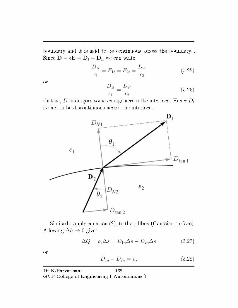
boundary and it is said to be continuous across the boundary .Since D = εE = Dt + Dn we can write
D1t
ε1= E1t = E2t =
D2t
ε2(5.25)
orD1t
ε1=D2t
ε2(5.26)
that is , D undergoes some change across the interface. HenceDt
is said to be discontinuous across the interface.
Similarly, apply equation (2), to the pillbox (Gaussian surface).Allowing ∆h→ 0 gives
∆Q = ρs∆s = D1n∆s−D2n∆s (5.27)
orD1n −D2n = ρs (5.28)
Dr.K.ParvatisamGVP College of Engineering ( Autonomous )
168

where ρs is the free charge density placed deliberately at theboundary. If no free charge exists at the interface ( ie., chargesare not placed deliberately placed at the interface) , ρs = 0 andthe equation becomes
D1n = D2n (5.29)
Thus the normal component ofD is continuous across the bound-ary. Since D = εE , the above equation can be written as
ε1E1n = ε2E2n (5.30)
showing that the normal component of E is discontinuous at theboundary. The above relations are collectively called the boundaryconditions; they must be satis�ed by an �eld at the boundaryseparating two di�erent dielectrics.
These conditions can be combined to show the change in thevectorsD and E at the interface. LetD1 and (E1) make an angleθ1 with the normal to the surface as shown in the �gure above.Since the normal components of D are continuous
DN1 = D1 cos θ1 = D2 cos θ2 = DN2 (5.31)
the ratio of tangential components is given by
Dtan1
Dtan2=D1 sin θ1
D2 sin θ2=ε1ε2
(5.32)
orε2D1 sin θ1 = ε2D2 sin θ2 (5.33)
Combining the equations
tan θ1
tan θ2=ε1ε2
(5.34)
In the above �gure , we have assumed that ε1 > ε2 , and thereforeθ1 > θ2 .
Dr.K.ParvatisamGVP College of Engineering ( Autonomous )
169
The direction of E on each side of the boundary is identicalwith the direction of D , because D = εE. The magnitude of Din region 2 may be found as
D2 = D1
√cos2 θ1 +
(ε2ε1
)2
sin2 θ1 (5.35)
and the magnitude of E2 is
E2 = E1
√sin2 θ1 +
(ε1ε2
)2
cos2 θ1 (5.36)
An inspection of these equations shows that D is larger in theregion of larger permittivity (unless θ1 = θ2 = 0 , where themagnitude is unchanged ) and that E is larger in the region ofsmaller permittivity ( unless θ1 = θ2 = 900 , where its magnitudeis unchanged). These boundary conditions, or the magnitude anddirection relations derived from them, allow us to �nd quickly the�eld on one side of the boundary if we know the �eld on the otherside.
5.0.3.2 Conductor - Dielectric Boundary:
This is the case shown in �gure below.
Dr.K.ParvatisamGVP College of Engineering ( Autonomous )
170

The conductor is assumed to be perfect. Although such a con-ductor is not practically realizable , we may regard conductorssuch as copper and silver as though they were perfect conduc-tors. To determine the boundary conditions for a conductor-dielectric interface , we follow the same procedure used for di-electric -dielectric interface except that we incorporate the factthat E = 0 inside the conductor. For the closed path abcda
0 = 0.∆w + 0.∆h
2+ En.
∆h
2− Et.∆w − En.
∆h
2− 0.
∆h
2(5.37)
as ∆h→ 0Et = 0 (5.38)
Similarly, for the pillbox letting ∆h→ 0 , we get
∆Q = Dn.∆s− 0.∆s (5.39)
because D = εE = 0 inside the conductor. Then
Dn =∆Q
∆s= ρs (5.40)
orDn = ρs (5.41)
Dr.K.ParvatisamGVP College of Engineering ( Autonomous )
171

Thus under static conditions , the following conclusions can bemade about a perfect conductor
1. No electric �eld may exist within a conductor : that is
ρs = 0 E = 0 (5.42)
2. Since E = −∇V = 0, there can be no potential di�erencebetween any two points in the conductor, that is a conductoris an equipotential surface.
3. The electric �eld E can be external to the conductor andnormal to the surface: that is
Dt = ε0εrEt = 0 Dn = ε0εrEn = ρs (5.43)
An important application of the fact that E = 0 inside a conduc-tor is in electrostatic screening or shielding.
If conductor A kept at zero potential surrounds conductor Bas shown in the �gure above , B is said to be electrostaticallyscreened by A from other electric systems such as C outside A .Similarly, Conductor C outside A is screened by A from b . The
Dr.K.ParvatisamGVP College of Engineering ( Autonomous )
172

conductor A acts like a screen or shield and the electrical condi-tions inside and outside the screen are completely independent ofeach other.
5.0.3.3 Conductor Free space Boundary Conditions
This is a special case of the conductor-dielectric conditions and isshown in the �gure below.
The boundary conditions at the interface between a conductorand free space can be obtained by replacing εr = 1 . We expectthe electric �eld E to be external to the conductor and normal toits surface. Thus the boundary conditions are
Dt = ε0Et = 0 Dn = ε0En = ρs (5.44)
it should be noted that the above equation implies that E �eldmust approach a conducting surface normally.
Dr.K.ParvatisamGVP College of Engineering ( Autonomous )
173

5.1. CAPACITANCE
5.1 Capacitance
A capacitor is an electrical device composed of two conductorswhich are separated by a dielectric medium and which can storeequal and opposite charges, independently of whether other con-ductors in the system are charged or not.
The capacitance between two conducting bodies is de�ned as
C =Q
V(5.45)
Q is charge in Coulombs and V is the potential di�erence betweenconducting bodies. When the capacitance of a single conductoris referred to, it is tacitly assumed that the other conductor is aspherical shell of in�nitely large radius.
Consider conductors 1 and 2 of arbitrary shape, as shown below
Dr.K.ParvatisamGVP College of Engineering ( Autonomous )
174

5.1. CAPACITANCE
Work is done on moving a charge from one conductor to theother. consequently a potential di�erence is established betweenthem. Conversely a P.D of V volts is applied between the con-ductors 1 and 2 , charges Q and −q will be built up on the con-ductors. there is a de�nite relationship between the charge andthe Potential di�erence and the ratio between the two is constant,determined from the geometrical con�guration of any particularsystem of conductors.
If a charge of 1 Coulomb is associated with a voltage of 1V ,the capacitance between the conductors is 1 Farad . 1 Farad is avery large quantity so capacitance is normally given in terms ofmicro, or pico Farads.
5.1.1 Parallel plate capacitor
Assume that the charge density on the plates is equal toρsC/m2
. The dielectric has ε = εrε0 , then
Dr.K.ParvatisamGVP College of Engineering ( Autonomous )
175

5.1. CAPACITANCE
D =ρs =Q
A
E =D
ε=
ρsεrε0
Potential di�erence between the plates is given by the integralof E over the separation of the plates d
V = Ed =ρsεrε0
(5.46)
C =Q
V=ρsAρsdεrε0
=εrε0d
(5.47)
5.1.2 Spherical Capacitor
E =Q
4πε0r2a < r < b
Vba =q
4πε0
[1
a− 1
b
]C =
Q
Vba=
4πε0[ 1a− 1b ]
=4πε0ab
(b− a)
as b −→∞ , C for an isolated sphere is 4πε0a Farads .
5.1.3 ENERGY STORED IN AN ELECTROSTATIC
FIELD:
The amount of work necessary to assemble a group of point chargesequals the total energy (We) stored in the resulting electric �eld.
Example (3 point charges): Given a system of 3 point charges,we can determine the total energy stored in the electric �eld of
Dr.K.ParvatisamGVP College of Engineering ( Autonomous )
176

5.1. CAPACITANCE
these point charges by determining the work performed to assem-ble the charge distribution. We �rst de�ne Vmn as the absolutepotential at Pm due to point charge Qn.
Figure 5.1: Energy to move point charges
1. Bring Q1 to P1(no energy required).
2. Bring Q2 to P2 (work = Q2V21).
3. Bring Q3 to P3 (work = Q3V31 +Q3V32)
The total work done We = 0 +Q2V21 +Q3V31 +Q3V32
If we reverse the order in which the charges are assembled, thetotal energy required is the same as before.
1. Bring Q3 to P3 (No energy required)
Dr.K.ParvatisamGVP College of Engineering ( Autonomous )
177

5.1. CAPACITANCE
2. Bring Q2 to P2 (work=Q2V23)
3. Bring Q1to P1 ( work done = Q1V12 +Q1V13)
Total work done We = 0 +Q2V23 +Q1V12 +Q1V13
Adding the above two equations
2We = Q1V12 +Q1V13 +Q2V21 +Q2V23 +Q3V31 +Q3V32 (5.48)
We =1
2[(Q1(V12 + V13) +Q2(V21 + V23) +Q3(V31 + V32)] =
1
2[Q1V1 +Q2V2 +Q2V3]
(5.49)where Vm is the total absolute potential at Pm a�ecting Qm.In general, for a system of N point charges, the total energy in
the electric �eld is given by
We =1
2
N∑k=1
QkVk (5.50)
For line, surface or volume charge distributions, the discretesum total energy formula above becomes a continuous sum (in-tegral) over the respective charge distribution. The point chargeterm is replaced by the appropriate di�erential element of chargefor a line, surface or volume distribution: ρLdL, ρsds or ρvdv. Theoverall potential acting on the point charge Qk due to the otherpoint charges (Vk) is replaced by the overall potential (v) actingon the di�erential element of charge due to the rest of the chargedistribution. The total energy expressions becomes
We =1
2
ˆ
L
ρLdL (Line Charge) (5.51)
Dr.K.ParvatisamGVP College of Engineering ( Autonomous )
178

5.1. CAPACITANCE
We =1
2
ˆ
s
ρsds (Surface Charge) (5.52)
We =1
2
ˆ
v
ρvdv (V olume Charge) (5.53)
If a volume charge distribution ρv of �nite dimension is enclosedby a spherical surface S0 of radius r0, the total energy
associated with the charge is given by
Figure 5.2: Distribution of volume charge
Dr.K.ParvatisamGVP College of Engineering ( Autonomous )
179
5.1. CAPACITANCE
We = limr0→∞
1
2
ˆ
v
ρvV dv
= limr0→∞
[1
2
ˆ(∇ •D)V dv
](5.54)
Using the following vector identity,
(∇ •D)V = ∇ • (V D)−D • ∇V (5.55)
the expression for the total energy can be written as
We = limr0→∞
1
2
ˆ
v
[∇ • (V D)]dv
− limr0→∞
1
2
ˆ
v
(D • ∇V )dv
(5.56)
If we apply the divergence theorem to the �rst integral, we �nd
We = limr0→∞
[1
2
‹V D • ds
]− lim
r0→∞
1
2
ˆ
v
(D • ∇V )dv
(5.57)
For each equivalent point charge (ρvdv) that makes up thevolume charge distribution, the potential contribution onS0 variesas r−1 and electric �ux density (and electric �eld) contributionvaries as r−2. Thus, the product of the potential and electric �uxdensity on the surface So varies as r−3. Since the integration overthe surface provides a multiplication factor of only r2, the surfaceintegral in the energy equation goes to zero on the surface S0 ofin�nite radius. This yields where the integration is applied overall space. The divergence term in the integrand can be written interms of the electric �eld as
E = −∇V (5.58)
Dr.K.ParvatisamGVP College of Engineering ( Autonomous )
180

5.2. CURRENT AND CURRENT DENSITY:
such that the total energy (J) in the electric �eld is
We =1
2
˚
v
D • Edv =1
2
˚
v
ε0(E • E)dv =1
2
˚
v
ε0E2dv
(5.59)This can also be expressed as
dWe
dv=
1
2ε0E
2 (5.60)
dWe
dv is called the energy density and is given in J/m3.
5.2 Current and Current density:
Electrical charges in motion constitute current. The unit of cur-rent is Ampere and is de�ned as the rate of movement of chargepassing a given reference point ( or passing a given reference plane) of one coulomb/sec. Current is denoted by I
I =dQ
dt(5.61)
Current is thus de�ned by the motion of the positive charges,even though conduction in metals takes place through the motionof electrons.
In �eld theory events occurring at a point, rather than withina small region are of interest, and the concept of current density,measured in Amperes/sq.m will be more useful. Current densityis a vector represented by J .
The increment of current ∆I crossing an incremental surfacearea ∆s normal to the current density is ∆I = JN4s and in thecase where the current density is not perpendicular to the surface,
∆I = J •∆s (5.62)
Dr.K.ParvatisamGVP College of Engineering ( Autonomous )
181

5.2. CURRENT AND CURRENT DENSITY:
Figure 5.3:
total current is obtained by integrating
I =
ˆ
s
J • ds (5.63)
current density is related to the velocity of volume charge den-sity at a point. Consider the element of charge
∆Q = ρv∆v = ρv∆s∆L (5.64)
let us assume that the charge element is oriented with its edgesparallel to the coordinate axes, and that it possesses only an xcomponent of velocity. In the time interval ∆t , the element ofcharge has moved a distance ∆x , as indicated in the �gure . Wehave therefore moved a charge∆Q = ρv∆s∆x through a referenceplane perpendicular to the direction of motion in a time increment∆t , and the resultant current is
∆I =∆Q
∆t= ρv∆s
∆x
∆t(5.65)
Dr.K.ParvatisamGVP College of Engineering ( Autonomous )
182
5.2. CURRENT AND CURRENT DENSITY:
in the limit as ∆t −→ 0 we have
∆I = ρv∆svx (5.66)
where vxis the velocity in the x− direction. In terms of the currentdensity
Jx = ρvvx (5.67)
and in generalJ − ρvv (5.68)
The above result shows very clearly that charge in motion con-stitutes a current . This type of current is called convection cur-rent density. The convection current density is related linearly tocharge density as well as to velocity.
5.2.1 Continuity Of current:
The principle of charge conservation states that charge can neitherbe created nor destroyed , although equal amounts of positiveand negative charge may be simultaneously created, obtained byseparation, destroyed or lost by recombination.
The continuity equation follows from this principle when weconsider any region bounded by a closed surface. The currentthrough the closed surface is
I =
‰J • ds (5.69)
and this outward �ow of positive charge must be balanced by adecrease of positive charge ( or perhaps an increase of negativecharge ) within the closed surface. if the charge inside the closedsurface is denoted by Q , then the rate of decrease is −dQi
dt andthe principle of charge conservation requires that
Dr.K.ParvatisamGVP College of Engineering ( Autonomous )
183

5.2. CURRENT AND CURRENT DENSITY:
I =
‰J • ds = −dQ
dt(5.70)
The above equation is the integral form of the continuity equation.The point form is obtained from the above by using the divergencetheorem.
‰J • ds =
ˆ
v
(∇ • J) dv
−dQdt
=− d
dt
ˆ
v
ρvdv = −ˆ
v
∂ρv∂t
dv
ˆ
v
(∇ • J) dv =−ˆ
v
∂ρv∂t
dv
This is true for any volume dv . This is possible only if theintegrands are equal. so
∇ • J = −∂ρ∂t
(5.71)
From the physical interpretation of divergence, the above equationindicates that the current or charge per second diverging from asmall volume per unit volume is equal to the time rate of decreaseof charge per unit volume at every point.
5.2.2 Ohm's Law: Point Form
Consider a conductor. the valance electrons , or conduction or freeelectrons , move under the in�uence of an electric �eld . With a�eld E , an electron having a charge Q = −e will experience aforce ,
F = −eE (5.72)
Dr.K.ParvatisamGVP College of Engineering ( Autonomous )
184

5.2. CURRENT AND CURRENT DENSITY:
In free space the electron will accelerate and continually increaseits velocity ( and energy ) . In the crystalline material the progressof the electron is impeded by continual collisions with the ther-mally excited crystalline lattice structure, and a constant averagevelocity is soon attained . This velocity Vd is termed as the driftvelocity and is linearly related to the electric �eld intensity by themobility of the electron in the given material. Mobility is denotedby µ
Vd = −µeE (5.73)
The electron velocity is in a direction opposite to the direction ofE . µe has the dimensions of square meter/Volt-second. Typicalvalues are
Aluminum 0.0012
Copper 0.0032
silver 0.0056
For good conductors a drift velocity of a few inches per secondis su�cient to produce a noticeable temperature rise and can causethe wire to melt if the heat can not be quickly removed by thermalconduction.
Substituting in JJ = −µeρeE (5.74)
The relationship between J and E for metallic conductors , is alsospeci�ed in terms of conductivity as
J = σE (5.75)
Dr.K.ParvatisamGVP College of Engineering ( Autonomous )
185

5.2. CURRENT AND CURRENT DENSITY:
where σ is in mho/m. The above relation is called the pointform of Ohm's law. The conductivity σ = −µeρ . The values ofconductivity for Aluminum, copper, and silver are
Aluminum 3.82× 10⁷
Copper 5.8× 10⁷
Silver 6.17× 10⁷
5.2.3 General Expression for Resistance
Dr.K.ParvatisamGVP College of Engineering ( Autonomous )
186

5.2. CURRENT AND CURRENT DENSITY:
I =
ˆ
s
J • ds
Vab =−aˆ
b
E • dL = −ELab
V =ELab = EL
J =I
s= σE = σ
V
L
I =σsV
LV
I=L
σs
When the �eld is nonuniform, the resistance is in general givenby
R =VabI
=−´ ab E • dl´
s σE • ds(5.76)
Dr.K.ParvatisamGVP College of Engineering ( Autonomous )
187

Unit-IV
Magnetostatics:
Static magnetic �elds � Biot-Savart's law � Oesterd's experi-ment - Magnetic �eld intensity (MFI) � MFI due to a straight cur-rent carrying �lament � MFI due to circular, square and solenoidcurrent � Carrying wire � Relation between magnetic �ux, mag-netic �ux density and MFI � Maxwell's second Equation,∇•B =0 .

Chapter 6
THE STEADY MAGNETIC
FIELD
Jean-Baptiste Biot (21 April 1774� 3 February 1862) was a Frenchphysicist, astronomer, and math-ematician who established the re-ality of meteorites, made an earlyballoon �ight, and studied thepolarization of light.Jean-BaptisteBiot was born in Paris, France on21 April 1774 and died in Paris on 3 February 1862. Biotserved in the artillery before he was appointed professorof mathematics at Beauvais in 1797. He later went onto become a professor of physics at the Collège de Francearound 1800, and three years later was elected as a mem-ber of the Academy of Sciences.
189

Félix Savart (30 June 1791 - 16March 1841) was the son of GérardSavart, an engineer at the mili-tary school of Metz. His brother,Nicolas, student at École Polytech-nique and o�cer in the engineer-ing corps, did work on vibration.At the military hospital at Metz,Savart studied medicine and laterhe went on to continue his studies at the University ofStrasbourg, where he received his medical degree in 1816[1]. Savart became a professor at Collège de France in1836 and was the co-originator of the Biot-Savart Law,along with Jean-Baptiste Biot. Together, they worked onthe theory of magnetism and electrical currents. Theirlaw was developed about 1820. The Biot-Savart Lawrelates magnetic �elds to the currents which are theirsources. Félix Savart also studied acoustics. He devel-oped the Savart wheel which produces sound at speci�cgraduated frequencies using rotating disks.
Dr.K.ParvatisamGVP College of Engineering ( Autonomous )
190
Hans Christian Ørsted (Danishpronunciation: [hans khKæsd
˚jan
"Œ5“sd˚
Eð]; often rendered Oerstedin English; 14 August 1777 � 9March 1851) was a Danish physi-cist and chemist who discoveredthat electric currents create mag-netic �elds, an important aspect ofelectromagnetism. He shaped post-Kantian philosophy and advancesin science throughout the late 19thcentury.[1]In 1824, Ørsted founded Selskabet for Naturlærens Ud-bredelse (SNU), a society to disseminate knowledge of thenatural sciences. He was also the founder of predecessororganizations which eventually became the Danish Meteo-rological Institute and the Danish Patent and TrademarkO�ce. Ørsted was the �rst modern thinker to explicitlydescribe and name the thought experiment.A leader of the so-called Danish Golden Age, Ørstedwas a close friend of Hans Christian Andersen andthe brother of politician and jurist Anders SandøeØrsted, who eventually served as Danish prime minister(1853�54).The oersted (Oe), the cgs unit of magnetic H-�eldstrength, is named after him.
Dr.K.ParvatisamGVP College of Engineering ( Autonomous )
191

6.0.1 INTRODUCTION:
We will begin our study of the magnetic �eld with the de�nitionof the magnetic �eld itself and show how it arises from a currentdistribution. The e�ect of this �eld on other currents, will also bediscussed.
The relation of the steady magnetic �eld to its source is morecomplicated than is the relation of the electrostatic �eld to itssource. It is necessary to accept several laws temporarily on faithalone. The proof of the laws does exist and can be covered at anadvanced level.
6.0.2 BIOT-SAVART LAW:
The source of steady magnetic �eld may be a permanent magnet,an electric �eld changing linearly with time , or a direct current.We shall largely ignore the permanent magnet and save the time-varying electric �eld for a later discussion. The present discussionwill be concerned about the magnetic �eld produced by a di�er-ential dc element in free space.
We may think of this di�erential current element as a vanish-ingly small section of a current carrying �lamentary conductor,where a �lamentary conductor is the limiting case of a cylindricalconductor of circular cross section as the radius approaches zero.We assume a current I �owing in a di�erential vector length of the�lament dL. The Biot-Savart law then states that at any pointP the magnitude of the magnetic �eld intensity produced by thedi�erential element is proportional to the product of the current, the magnitude of the di�erential length, and the sine of the an-gle lying between the �lament and a line connecting the �lamentto the point P where the �eld is desired. The magnitude of the
Dr.K.ParvatisamGVP College of Engineering ( Autonomous )
192

magnetic �eld intensity is inversely proportional to the square ofthe distance from the di�erential element to the point P . Thedirection of the magnetic �eld intensity is normal to the planecontaining the di�erential �lament and the line drawn from the�lament to the point P . Of the two possible two normals, thatone is two be chosen which is in the direction of progress of aright handed screw turned from dL through the smaller angle tothe line from the �lament P . The proportionality constant is 1
4π
.This can be written concisely using vector notation as
dH =IdL× aR
4πR2=IdL×R
4πR3(6.1)
The units of magnetic �eld intensityH are evidently amperes permeter (A/m ). The geometry is illustrated in the �gure below.
Figure 6.1: Biot-Savart Law
Dr.K.ParvatisamGVP College of Engineering ( Autonomous )
193

If the current element ( source point ) is indicated by 1 andthe �eld point P is indicated by 2 , then
dH2 =I1dL1 × aR12
4πR212
(6.2)
It is impossible to check Biot-Savart law in the above form becausethe di�erential current element cannot be isolated and it is anidealization. Only the integral form of the law can be veri�edexperimentally.
H =
˛IdL× aR
4πR2(6.3)
The direction of H can be determined by the right hand rulewith the right hand thumb pointing in the direction of the current, then the right hand �ngers encircling the wire show the directionof H as shown in the �gure. Alternatively , we can use the righthand screw ruleto getermine the direction of H. With the screwplaced along the wire and pointed in the direction of the current�ow, the direction of advance of the screw is the direction ofH.
Dr.K.ParvatisamGVP College of Engineering ( Autonomous )
194

It is customary to represent the direction of the magnetic �eldintensity H ( or current I ) by a small circle with a dot or crosssign depending on whether H ( or I ) is out of, or into the pageas illustrated in the �gure.
The Biot-Savart law can also be expressed in terms of dis-tributed sources, such as current density J and surface currentdensity K . Surface current �ows in a sheet of vanishingly smallthickness , and the current density J , measured in amperes /
Dr.K.ParvatisamGVP College of Engineering ( Autonomous )
195
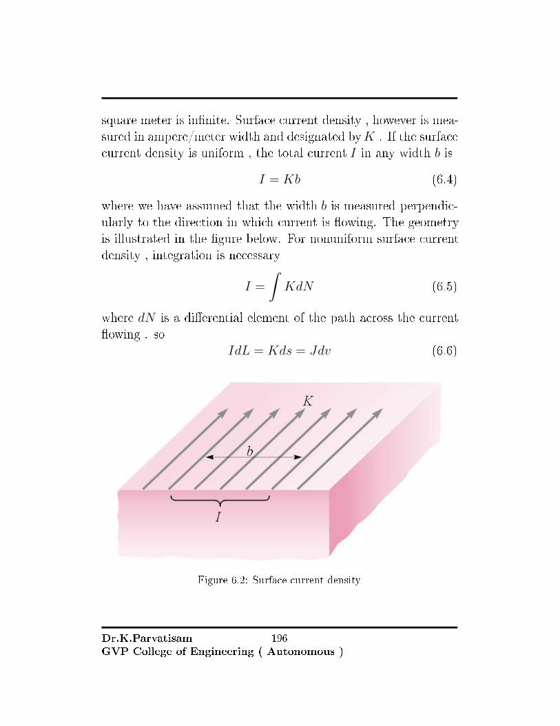
square meter is in�nite. Surface current density , however is mea-sured in ampere/meter width and designated byK . If the surfacecurrent density is uniform , the total current I in any width b is
I = Kb (6.4)
where we have assumed that the width b is measured perpendic-ularly to the direction in which current is �owing. The geometryis illustrated in the �gure below. For nonuniform surface currentdensity , integration is necessary
I =
ˆKdN (6.5)
where dN is a di�erential element of the path across the current�owing . so
IdL = Kds = Jdv (6.6)
Figure 6.2: Surface current density
Dr.K.ParvatisamGVP College of Engineering ( Autonomous )
196

Biot-Savart law can be expressed in terms of current densitiesas
H =
ˆ
s
K × aRds4πR2
H =
ˆ
vol
J × aR4πR2
Line current, surface current and volume current distributionsare shown in the �gure below.
6.0.3 FIELD BECAUSE OF A FINITE LINE CUR-
RENT:
The �gure below shows a �nite length �lamentary current
Dr.K.ParvatisamGVP College of Engineering ( Autonomous )
197

Figure 6.3: The magnetic �eld intensity caused by a �nite length �lament
Using Biot-Savart law
Dr.K.ParvatisamGVP College of Engineering ( Autonomous )
198

dH =Idz
′az × [ρaρ + (z − z′)az]4π [ρ2 + (z − z′)2]
32
dH =I
4π
ρdz′
[ρ2 + (z − z′)2]32
aφ
dH = − I
4π
ρ2 sec2 αdα
ρ3 sec3 αaφ
H =I
4πρ
α1ˆ
α2
(− cosα)dαaφ
H =I
4πρ(sinα2 − sinα1) aφ
For an in�nitely long conductor
α2 = 900 , α1 = −900 (6.7)
resulting in
H =I
2πρaφ (6.8)
The magnitude of the �eld is not a function of φ or z and it variesinversely as the distance from the �lament. The direction of themagnetic �eld intensity vector is circumferential. The stream-lines are therefore circles about the �lament, and the �eld may bemapped in cross section as shown in �gure below
Dr.K.ParvatisamGVP College of Engineering ( Autonomous )
199

Figure 6.4: Streamlines of the magnetic �eld_in�nitely long conductor
A comparison with the map of the electric �eld about an in�-nite line charge shows that the streamlines of the magnetic �eldcorrespond exactly to the equipotentials of the electric �eld, andunnamed perpendicular family of curves in the magnetic �eld cor-respond to the streamlines of the electric �eld.
Example;Determine H at P2(0.4, 0.3, 0) in the �eld of an 8 − A �la-
mentary current directed inward from in�nity to the origin on thepositive x−axis and outward to in�nity along the y−axis . Thearrangement is shown in the �gure.
Dr.K.ParvatisamGVP College of Engineering ( Autonomous )
200

Figure 6.5:
Solution:First consider the semi-in�nite current on thex−axis, and iden-
tify the two angles ,α1x = −900 and α2x = arctan(0.40.3) = 53.10 .
The radial distance ρ is measured from the x− axis , and we haveρx = 0.3 . Thus the contribution to H2 is
H2x =8
4π(0.3)(sin 53.10 + 1)aφ =
12
πaφ (6.9)
The unit vector aφ must also be referred to the x− axis . We seethat this is −az . Therefore
H2x = −12
πaz A/m (6.10)
Dr.K.ParvatisamGVP College of Engineering ( Autonomous )
201

For the current on the y− axis , we have α1y = − arctan(0.30.4) =
−36.90 and ρy = 0.4 . It follows that
H2y =8
4π(0.4)
(1 + sin 36.90
)(−az) = −8
πaz A/m (6.11)
Adding these results , we have
H2 = H2x +H2y = −20
πaz = −6.37az A/m (6.12)
6.0.4 MAGNETIC FIELD AT ANY POINT ON THE
AXIS OF A CIRCULAR CURRENT LOOP:
Consider a circular current carrying loop shown in �gure below
Figure 6.6: a)Circular current loop b)Flux lines due to current loop
Dr.K.ParvatisamGVP College of Engineering ( Autonomous )
202

R = haz − ρaρaR =
haz − ρaρ√[h2 + ρ2]
dH =Iρdφaφ × (haz − ρaρ)
4π [h2 + ρ2]32
=Iρhaρdφ
4π [h2 + ρ2]32
+Iρ2azdφ
4π [h2 + ρ2]32
H =
2πˆ
0
[Iρhaρdφ
4π [h2 + ρ2]32
+Iρ2azdφ
4π [z2 + ρ2]32
]= 0 +
I
4π
2πˆ
0
Iρ2azdφ
4π [h2 + ρ2]32
H =I
2
ρ2
[h2 + ρ2]32
az
Field at the center (h = 0) is
H =I
2ρaz (6.13)
6.0.5 MAGNETIC FIELD AT ANY POINT ON THE
AXIS OF A LONG SOLENOID:
A solenoid of length l and radius a consists of Nturns of wire andcarries a current of Iamps.
Dr.K.ParvatisamGVP College of Engineering ( Autonomous )
203

Figure 6.7: Cross section of a solenoid
Consider the cross section of the solenoid as shown in the �gureabove. Since the solenoid consists of circular loops , we apply theresult of the circular loopto �nd the �eld. The contribution to the�eld H at P by an element of the solenoid of length dz is
dH =Idla2
2 [a2 + z2]32
=Ia2ndz
2 [a2 + z2]32
(6.14)
where dl = ndz =(nl
)dz . From the �gure
tan θ =a
z
dz = −acosec2θdθ =−[z2 + a2
] 32
a2sin θdθ
Hence
dHz = −nI2
sin θdθ (6.15)
thus
Hz = −θ2ˆ
θ1
sin θdθ (6.16)
Dr.K.ParvatisamGVP College of Engineering ( Autonomous )
204

6.1. MAGNETIC FLUX AND MAGNETIC FLUX DENSITY:
H =nI
2(cos θ2 − cos θ1) az (6.17)
substituting n = NIL
H =NI
2L(cos θ2 − cos θ1) az (6.18)
at the center of the solenoid
cos θ2 =L2[
a2 + L2
4
] 12
= − cos θ1 (6.19)
and
H =NI
Lcos θ2az (6.20)
If L >> a or θ2 = 00 , θ1 = 1800
H =NI
Laz (6.21)
6.1 MAGNETIC FLUXANDMAGNETIC FLUX
DENSITY:
In frre space let us de�ne the magnetic �ux density B as
B = µ0H (6.22)
whereB is measured in Webers/square meter (Wb/m2) or in Tesla( T ).The constant µ0 is not dimensionless and has the value
µ0 = 4π × 10−7 H/m (6.23)
This called the permeability of free space.The magnetic �ux density vector B , as the name implies, is a
member of the �uxdensity family of vector �elds.
Dr.K.ParvatisamGVP College of Engineering ( Autonomous )
205

6.1. MAGNETIC FLUX AND MAGNETIC FLUX DENSITY:
If we represent magnetic �ux by φ and de�ne φ as the �uxpassing through any designated area
φ =
ˆ
s
B • ds Wb (6.24)
For electrical �ux the charge Q is the source of the �eld and the�ux lines begin and terminate on positive and negative charge,respectively.
No such source has ever been discovered for the lines of mag-netic �ux . The magnetic �ux lines are closed and do not terminateon a magnetic charge . For this reason Gauss's law for magnetic�eld is ˛
s
B • ds = 0 (6.25)
Applying divergence theorem we get
∇ •B = 0 (6.26)
The above is not a proof but we have merely shown the truth.This can also be shown starting from the Biot-Savart law. As-
sume that point 1 is the source point and point 2is the �eld point .Then Biot-Savart law in terms of volume current dnesity is givenby
B2 =µ0
4π
ˆ
v
J1 ×R12
|R12|3dv1 (6.27)
Then
∇2 •B2 = ∇2 •
ˆv
J1 ×R12
|R12|3dv1
(6.28)
Dr.K.ParvatisamGVP College of Engineering ( Autonomous )
206

6.1. MAGNETIC FLUX AND MAGNETIC FLUX DENSITY:
from the vector identity
∇ • (x× y) = −x • ∇ × y + y • ∇x (6.29)
here
x = J1 , y =R12
|R12|3(6.30)
So using the above relation
∇2•B2 =µ0
4π
ˆ
v
[−J1 • ∇2 ×
(R12
|R12|3)
+R12
|R12|3• ∇2 × (J1)
]dv1
(6.31)
∇2•B2 =µ0
4π
ˆ
v
[−J1 • ∇2 ×∇2
(− 1
R12
)+
R12
|R12|3• ∇2 × (J1)
]dv1
(6.32)But
∇2 ×∇2
(− 1
R12
)= 0 (6.33)
as curl of gradient of any function is zero. Also
∇2 × (J1) = 0 (6.34)
as J! is a function of coordinates of point 1 and cul is taken withrespect to the coordinates of point 2 . So
∇2 •B2 = 0 or in general ∇ •B = 0 (6.35)
The equations above are the Maxwell's equation for the steadymagnetic �eld in integral form and di�erential or point form.
Dr.K.ParvatisamGVP College of Engineering ( Autonomous )
207

6.1. MAGNETIC FLUX AND MAGNETIC FLUX DENSITY:
Collecting all the equations , both for static electric �elds andsteady magnetic �elds we have
MAXWELL'S EQUATIONS
(STATIC FIELDS)
INTEGRAL FORMDIFFERENTIAL
ORPOINT FORM
¸sD • ds =
´vρvdv ∇ •D = ρv
¸lE • dl = 0 ∇× E = 0
¸sB • ds = 0 ∇ •B = 0
¸lH • dl =
¸sJ • ds ∇×H = J
Table 6.1: Maxwell's Equations For Static Electromagnetic Field
We will add the following equations for completeness
D = ε0E
B = µ0H
E = −∇V
Dr.K.ParvatisamGVP College of Engineering ( Autonomous )
208

Unit-V
Ampere's circuital law and its applications:
Ampere's circuital law and its applications viz. MFI due toan in�nite sheet of current and a long current carrying �lament �Point form of Ampere's circuital law � Maxwell's third equation,Curl (H)=Jc, Field due to a circular loop, rectangular and squareloops.

210

Chapter 7
AMPERE'S CIRCUITAL LAW:
André-Marie Ampère (20 January1775 � 10 June 1836) was a Frenchphysicist and mathematician whois generally regarded as one of themain founders of the science ofclassical electromagnetism, whichhe referred to as "electrodynam-ics". The SI unit of measurementof electric current, the ampere, isnamed after him.Ampère was born on 20 January 1775to Jean-Jacques Ampère, a prosperousbusinessman, and Jeanne Antoinette Desutières-Sarcey Ampèreduring the height of the French Enlightenment. He spent hischildhood and adolescence at the family property at Poleymieux-au-Mont-d'Or near Lyon.[1] Jean-Jacques Ampère, a successfulmerchant, was an admirer of the philosophy of Jean-JacquesRousseau, whose theories of education (as outlined in his treatiseÉmile) were the basis of Ampère's education. Rousseau believedthat young boys should avoid formal schooling and pursue insteadan �education direct from nature.� Ampère's father actualized thisideal by allowing his son to educate himself within the walls ofhis well-stocked library. French Enlightenment masterpieces suchas Georges-Louis Leclerc, comte de Bu�on's Histoire naturelle,générale et particulière (begun in 1749) and Denis Diderot andJean le Rond d'Alembert's Encyclopédie (volumes added between1751 and 1772) thus became Ampère's schoolmasters. The youngAmpère, however, soon resumed his Latin lessons, which enablehim to master the works of Leonhard Euler and Daniel Bernoulli.
Dr.K.ParvatisamGVP College of Engineering ( Autonomous )
211

Ampere's circuital law states that the line integral ofH aroundany closed path is exactly equal to the direct current enclosed bythat path.
˛H • dl = I (7.1)
We de�ne positive current as �owing in the direction of advance ofa right-handed screw turned in the direction in which the closedpath is traversed.
Figure 7.1: Ampere's Circuital Law
The �gure shows a circular wire carrying a direct current I, the line integral of H about the closed paths lettered a and bresults in an answer of I ; the integral of the closed path c whichpasses through the conductor gives an answer less than I and isexactly that portion of the total current which is enclosed by the
Dr.K.ParvatisamGVP College of Engineering ( Autonomous )
212

path c . Although the paths a and b give the same answer , theintegrands are , of course, di�erent. The line integral directs usto multiply the component of H in the direction of the path bya small increment of path length at one point of the path, movealong the path to the next incremental length, and repeat theprocess , continuing until the path is completely traversed. SinceH will in general vary from point to point , and since paths a andb are not alike , the contributions to the integral made by, say ,each millimeter of path length are quite di�erent. Only the �nalanswers are the same.
We should also consider exactly what is meant by the expres-sion �current enclosed by the path� . Suppose we solder a circuittogether after passing the conductor once through a rubber band ,which we shall use to represent the closed path. Some strange andformidable paths can be constructed by twisting and knotting therubber band , but if neither the rubber band nor the conductingcircuit is broken , the current enclosed by the path is that carriedby the conductor. Now let us replace the rubber band by a cir-cular ring of spring steel across which is stretched a rubber sheet.The steel loop forms the closed path, and the current conductormust pierce the rubber sheet if the current is to be enclosed by thepath. Again, we may twist the steel loop, and we may also deformthe rubber sheet by pushing our �st into it or folding it in anyway we wish. A single current carrying conductor still pierces thesheet once, and this is the true measure of the current enclosedby the path. If we thread the conductor once through the sheetfrom front to back and once from back to front , the total currentenclosed by the path is the algebraic sum, which is zero.
In more general language, given a closed path, we recognize thispath as the perimeter of an in�nite number of surfaces ( not closed
Dr.K.ParvatisamGVP College of Engineering ( Autonomous )
213

surfaces ). Any current carrying conductor enclosed by the pathmust pass through every one of these surfaces once. certainly someof the surfaces may be chosen in such a way that the conductorpierces them twice in one direction and once in the other direction,but the algebraic sum of the current is still the same.
We shall �nd that the closed path is usually of an extremelysimple nature and can be drawn on a plane. We need merely �ndthe total current passing through this region of the plane.
7.0.1 APPLICATIONS:
7.0.1.1 INFINITELY LONG FILAMENT:
Consider an in�nitely long �lamentary conductor carrying a cur-rent I A . The �lament lies on the z− axis in free space, and thecurrent �ows in the direction of az. Symmetry shows that there isno variation with z or φ . Using Biot-Savart law, the direction ofdH is perpendicular to the plane containing dL and R and there-fore is in the direction of aφ . Hence the only component of HisHφ and it is a function only of ρ .
The path chose should be a circle of radius ρ and Ampere'scircutal law becomes
˛H • dl =
2πˆ
0
Hφρdφ = Hφ2πρ = I (7.2)
or
Hφ =I
2πρ(7.3)
as before.
Dr.K.ParvatisamGVP College of Engineering ( Autonomous )
214

7.0.1.2 INFINITELY LONG COAXIAL TRANSMISSION LINE:
Consider an in�nitely long coaxial transmission line carrying auniformly distributed total current I in the center conductor and−I in the outer conductor. The line is shown in the �gure below.
Figure 7.2: Coaxial transmission Line
Symmetry shows that H is not a function of φ or z . In or-der to determine the components present, we may use the resultsof the previous example by considering solid conductors as be-ing composed of large number of �laments. No �lament has a zcomponent of H . Furthermore, the Hρ component at φ = 0 ,produced by one �lament located at ρ = ρ1, φ = φ1 , is canceledby the Hρ component produced by a symmetrically located atρ = ρ1, φ = −φ1 . So only an Hφ component which varies with ρremains.
A circular path of radius ρ , where ρ is larger than the radiusof the inner conductor but less than the inner radius of the outer
Dr.K.ParvatisamGVP College of Engineering ( Autonomous )
215

conductor, then leads immediately to
Hφ =I
2πρ(a < ρ < b) (7.4)
If we chose ρ smaller than the radius of the inner conductor, thecurrent enclosed is
Iencl = Iρ2
a2(7.5)
and
2πρHφ = Iρ2
a2(7.6)
or
Hφ =Iρ
2πa2(ρ < a) (7.7)
If the radius ρ is larger than the outer radius of the outer conduc-tor , no current is enclosed and
Hφ = 0 (ρ > c) (7.8)
Finally, if the path lies within the outer conductor , we have
2πρHφ = I − I(ρ2 − b2
c2 − b2
)Hφ =
I
2πρ
c2 − ρ2
c2 − b2(b < ρ < c)
The magnetic �eld strength variation with radius is shown in the�gure given below.
Dr.K.ParvatisamGVP College of Engineering ( Autonomous )
216
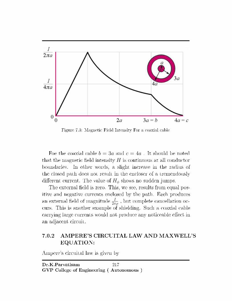
Figure 7.3: Magnetic Field Intensity For a coaxial cable
Foe the coaxial cable b = 3a and c = 4a . It should be notedthat the magnetic �eld intensityH is continuous at all conductorboundaries. In other words, a slight increase in the radius ofthe closed path does not result in the encloser of a tremendouslydi�erent current. The value of Hφ shows no sudden jumps.
The external �eld is zero. This, we see, results from equal pos-itive and negative currents enclosed by the path. Each producesan external �eld of magnitude I
2πρ , but complete cancellation oc-curs. This is another example of shielding. Such a coaxial cablecarrying large currents would not produce any noticeable e�ect inan adjacent circuit.
7.0.2 AMPERE'S CIRCUITAL LAWANDMAXWELL'S
EQUATION:
Ampere's circuital law is given by
Dr.K.ParvatisamGVP College of Engineering ( Autonomous )
217

˛H • dl = Ienc (7.9)
Ampere's law is similar to Gauss's law and it is easily appliedto determine H when the current distribution is symmetrical. Itshould be noted that the above equation always holds whether thecurrent distribution is symmetrical or not but we can only use theequation to determine H when symmetrical current distributionexists. Ampere's law is a special case of Biot-Savart law; theformer may be derived from the latter.
By applying Stoke's theorem to the left hand side of the aboveequation , we obtain
Ienc =
˛
L
H • dl =
ˆ
s
(∇×H) • ds but I =
ˆ
encs
J • ds (7.10)
Comparing the surface integrals , we get
∇×H = J (7.11)
This is third of the Maxwell's equations. It is essentially Am-pere's law in di�erential or point form. As the curl of J is notequal to zero, the magnetostatic �eld is not a conservative �eld.The integral form of the equation is given by
˛
L
H • dl =
ˆ
s
J • ds (7.12)
The di�erential and integral forms of the Maxwell's equation forstatic magnetic �eld is given by
Dr.K.ParvatisamGVP College of Engineering ( Autonomous )
218

∇×H = J (7.13)
˛
L
H • dl =
ˆJ • ds (7.14)
(7.15)
7.0.2.1 Applications Of Ampere's Circuital Law
We now apply Ampere's circuital law to determine H for sym-metrical current distributions as we did for Gauss's law. We willconsider an in�nite line current , an in�nite current sheet.In�nite Line current:
Consider an in�nitely long �lamentary current I along the z−axis as in the �gure below. To determine H at an observationpoint P , we allow a closed path pass through P .This path, onwhich Ampere's law is to be applied is known as Amperian path.We choose a concentric circle as the Amperian path in view of thenature of the problem which says thatH is constant provided ρ isconstant . Since this path encloses the whole current I , accordingto Ampere's law
I =
ˆHφaφ • ρdφaφ = Hφ
ˆρdφ = Hφ.2πρ (7.16)
or
H =I
2πρaφ (7.17)
In�nite Sheet Of Current:
Consider an in�nite sheet in the z = 0 plane. If the sheet hasa uniform current density k =kyay A/m as shown in �gure, then
Dr.K.ParvatisamGVP College of Engineering ( Autonomous )
219

applying Ampere's circuital law to the rectangular closed path (Amperian path ) gives˛
H • dl = Ienc = kyb (7.18)
To evaluate the integral , we �rst need to have an idea of whatHis like.To achieve this, we regard the in�nite sheet as comprising of�laments; dH above or below the sheet due to a pair of �lamentarycurrents can be found . As evident in the �gure , the resultantdH has only an x− component. Also , H one side of the sheetis the negative of that on the other side . Due to the in�niteextent of the sheet , the sheet can be regarded as consisting ofsuch �lamentary pairs so that the characteristics ofH for a pairare the same for the in�nite current sheets, that is
H =
{H0ax z > 0
−H0ax z < 0(7.19)
where H0 is yet to be determined . Evaluating the line integral ofH along the closed path gives
Dr.K.ParvatisamGVP College of Engineering ( Autonomous )
220

˛H • dl =
2ˆ
1
+
3ˆ
2
+
4ˆ
3
+
1ˆ
4
H • dl
=0(−a) + (−H0)(−b) + 0(a) +H0(b)
=2H0b
From the above relations , we obtain H0 = 12ky . Substituting
H =
{12kyax z > 0
−12kyax z > 0
(7.20)
In general , for an in�nite sheet of current density k A/m
H =1
2k× an (7.21)
where anis the unit normal vector directed from the current sheetto the point of interest.
Dr.K.ParvatisamGVP College of Engineering ( Autonomous )
221

Unit-VI
Force in magnetic �elds:
Magnetic force - Moving charges in a Magnetic �eld � Lorentzforce equation � force on a current element in a magnetic �eld� Force on a straight and a long current carrying conductor ina magnetic �eld � Force between two straight long and parallelcurrent carrying conductors � Magnetic dipole and dipole moment� a di�erential current loop as a magnetic dipole � Torque on acurrent loop placed in a magnetic �eld

223

Chapter 8
MAGNETIC FORCES,
MATERIALS, AND
INDUCTANCE
Hendrik Antoon Lorentz (Arnhem, 18July 1853 � Haarlem, 4 February 1928)was a Dutch physicist who shared the1902 Nobel Prize in Physics with PieterZeeman for the discovery and theoreti-cal explanation of the Zeeman e�ect. Healso derived the transformation equa-tions subsequently used by Albert Ein-stein to describe space and time.Hendrik Lorentz was born in Arnhem, Gelderland (The Nether-lands), the son of Gerrit Frederik Lorentz (1822�1893), a well-o�nurseryman, and Geertruida van Ginkel (1826�1861). In 1862,after his mother's death, his father married Luberta Hupkes. De-spite being raised as a Protestant, he was a freethinker in religiousmatters.[B 1] From 1866 to 1869 he attended the newly estab-lished high school in Arnhem, and in 1870 he passed the examsin classical languages which were then required for admission toUniversity.Lorentz studied physics and mathematics at the University of Lei-den, where he was strongly in�uenced by the teaching of astron-omy professor Frederik Kaiser; it was his in�uence that led himto become a physicist.
Dr.K.ParvatisamGVP College of Engineering ( Autonomous )
224

8.0.1 FORCE ON A MOVING CHARGE:
In an electric �eld the de�nition of the �eld intensity shows usthat the force on a charged particle is
F = QE (8.1)
The force is in the same direction as the electric �eld intensity (fora positive charge) and is directly proportional to both E and Q .If the charge is in motion, the force at any point in its trajectoryis given by the above equation.
A charged particle in motion in a magnetic �eld of �ux densityB is found experimentally to experience a force whose magnitudeis proportional to the product of the magnitudes of the chargeQ, its velocity v , and the �ux density B , and to the sine of theangle between the vectors v and B . The direction of the force isis perpendicular to both v and B and is given by the unit vectorin the direction of v ×B . The force therefore is expressed as
F = Qv ×B (8.2)
The force on a moving particle due to combined electric and mag-netic �elds is obtained by superposition as
F = Q(E + v ×B) (8.3)
The equation is known as the Lorentz's force equation, and itssolution is required in determining electron orbits in the mag-netron, proton paths in the cyclotron, plasma characteristics in amagnetohydrodynamic (MHD) generator, or , in general , chargedparticle motion in combined electric and magnetic �elds.
Dr.K.ParvatisamGVP College of Engineering ( Autonomous )
225

8.0.2 FORCE ON A DIFFERENTIAL CURRENT EL-
EMENT:
The force on a charged particle moving through a steady mag-netic �eld may be written as the di�erential force exerted on adi�erential element of charge,
dF = dQv ×B (8.4)
The di�erential element of charge may also be expressed in termsof volume charge density ,
dQ = ρvdv (8.5)
thusdF = ρvdv v ×B (8.6)
ordF = J ×Bdv (8.7)
but we know that Jdv = Kds = IdL and thus the Lorentz's forceequation may be applied to surface current density
dF = K ×Bds (8.8)
or to a di�erential current �lament
dF = IdL×B (8.9)
Integrating the above equations over a volume, surface, or a closedpath , respectively , leads to the integral formulations
F =
ˆ
vol
J ×Bdv
F =
ˆ
s
K ×Bds
Dr.K.ParvatisamGVP College of Engineering ( Autonomous )
226

and
F =
˛
l
IdL×B = −I˛
l
B × dL (8.10)
A simple result is obtained by applying the last equation to astraight conductor in a uniform magnetic �eld
F = IL×B (8.11)
The magnitude of the force is given by the familiar equation
F = BIL sin θ (8.12)
where θ is the angle between the vectors representing the directionof current �ow and the direction of the magnetic �ux density.
Example:Consider the �gure below.
Figure 8.1: Square Loop Of Wire In The xy-plane
Dr.K.ParvatisamGVP College of Engineering ( Autonomous )
227

We have a square loop of wire in the z = 0 plane carrying2mA of current in the �eld of an in�nitely long �lament on they − axis . The �eld produced in the plane of the loop by thestraight �lament is
H =I
2πxaz =
15
2πxaz A/m (8.13)
therefore
B = µ0H = 4π × 10−7H =3× 10⁻⁶
xaz T (8.14)
Then
F = −˛B × dL (8.15)
Let us assume a rigid loop so that the total force is the sum of theforces on the four sides. Beginning with the left side:
F = −2× 10−3 × 3× 10−6
3ˆ
x=1
azx× dxax +
3ˆ
y=1
az3× dyay +
1ˆ
x=3
azx× dxax +
1ˆ
y=3
az1× dyay
F = −6× 10⁻⁹
[ln|31 ay +
1
3y
∣∣∣∣31
(−ax) + lnx|13 ay + y|13 (−ax)]
F = −6× 10⁻⁹
[(ln 3)ay −
2
3ax +
(ln
1
3
)ay + 2ax
]= −8ax pN
Thus the net force on the loop is in the −ax direction.
8.0.3 FORCE BETWEENDIFFERENTIAL CURRENT
ELEMENTS:
It is possible to express the force on one current element directlyin terms of a second current element without �nding the magnetic
Dr.K.ParvatisamGVP College of Engineering ( Autonomous )
228

�eld. The magnetic �eld at point 2 due to a current element atpoint 1 has been found to be
dH2 =I1dL1 × aR12
4πR212
(8.16)
Now, the di�erential force on a di�erential current element is
dF = IdL×B (8.17)
and we apply this to our problem by lettingB be dB2 (the di�er-ential �ux density at point 2 caused by current element at 1 ) ,by identifying IdL as I2dL2 , and by symbolizing the di�erentialof our di�erential force on element 2 as d(dF2)
d(dF2) = I2dL2 × dB2 (8.18)
since dB2 = µ0dH2 , we obtain the force between two di�erentialcurrent elements ,
d(dF2) = µ0I1I2
4πR212
dL2 × (dL1 × aR12) (8.19)
Example:Consider two di�erential current elements shown in the �gure.
I1dL1 = −3ay A.m at P1(5, 2, 1) , and I2dL2 = −4azA.m atP2(1, 8, 5) .
Dr.K.ParvatisamGVP College of Engineering ( Autonomous )
229

Figure 8.2: Force Between Two Current Elements
Thus R12 = −4ax + 6ay + 4az , and we may substitute thisdata in the equation resulting in
d(dF2) =4π × 10−7
4π
(−4az)× [(−3ay)× (−4ax + 6ay + 4az)]
(16 + 36 + 16)1.5= 8.56ay nN
(8.20)If we �nd d(dF1) it is equal to −12.8az nN which is not equaland opposite to the force d(dF2) . The reason for this is that adi�erential current element is an abstraction, and it can not existin practice. The continuity of current demands that a completecircuit be considered .
So the total force between two �lamentary circuits is obtained
Dr.K.ParvatisamGVP College of Engineering ( Autonomous )
230

by integrating twice:
F2 = µ0I1I2
4π
˛ [dL2 ×
˛dL1 × aR12
R212
]F2 = µ0
I1I2
4π
˛ [˛aR12× dL1
R212
]× dL2
The above equation, though appears to be formidable, it is not dif-�cult to use. It can be used to �nd the force between two in�nitelylong, straight , parallel, �lamentary conductors with separation d, and carrying equal but opposite currents.
E:/Data_Parva/Desktop(11-10-2011)/eee_electromagnetics/parallel_currents.png
The magnetic �eld intensity at either wire caused by the otheris already known to be I
2πd . it can be seen that the force is
µ0I2
2πdnewtons per meter length. (8.21)
This can be derived in a di�erent way as shown below
E:/Data_Parva/Desktop(11-10-2011)/eee_electromagnetics/parallel_currents.eps
Dr.K.ParvatisamGVP College of Engineering ( Autonomous )
231

F1 =µ0I1I2
4π
˛ ˛dl1 × (dl2 × aR)
R2N
=
˛ ˛(µ0I1dl1) (I2dl2 cos θ)
4πR2
R = d sec θ,l2 = d tan θ, dl2 = d sec2 θdθ
=µ0I1I2
4πd
1ˆ
0
dl1
π2ˆ
−π2
cos θdθ
F1 =µ0I1I2
2πdN/m
8.0.4 FORCE AND TORQUE ON A CLOSED CIR-
CUIT:
The force on a �lamentary closed circuit is given by
F = −I˛B × dL (8.22)
If we assume that the magnetic �eld is uniform , then B can beremoved from the integral
F = −IB ײdL (8.23)
but the closed line integral¸dL = 0 . Therefore the force on a
closed �lamentary circuit in a uniform magnetic �eld is zero. Ifthe �eld is not uniform , the total force need not be zero.
Although the force is zero, the torque is generally not zero. Indetermining the torque , or moment , of a force , it is necessaryto consider both an origin at or about which the torque is to becalculated as well as the point at which the force is applied. Seethe �gure below:
Dr.K.ParvatisamGVP College of Engineering ( Autonomous )
232

Figure 8.3:
We apply a force F at point P , and we establish an origin atO with a rigid lever arm Rextending from O to P . The torqueabout point O is a vector whose magnitude is the product of themagnitudes ofR and F , and of the sine of the angle between thesetwo vectors. The direction of the vector torqueT is normal to boththe force F and lever arm R and is in the direction of progressof a right handed screw as the lever arm is rotated into the forcevector through the smaller angle . The torque is expressible as across product
T = R× F (8.24)
Now let us assume that two forces , F1 at P1 and F2 at P2 ,having lever arms R1 and R2 extending from a common origin O, as shown in the �gure are applied to an object of �xed shapeand that the object does not undergo any translation. The torqueabout the origin is
T = R1 × F1 +R2 × F2 (8.25)
Dr.K.ParvatisamGVP College of Engineering ( Autonomous )
233

whereF1 + F2 = 0 (8.26)
and therefore
T = (R1 −R2)× F1 = R21 × F1 (8.27)
The vector R21 = R1 − R2 joins the point of application of F2 tothat of F1 and is independent of the choice of origin for the twovectors R1 and R2 . Therefore the torque is also independent ofthe choice of origin, provided that the total force is zero.
We may therefore choose the most convenient origin , and thisis usually on the axis of rotation and in the plane containing theapplied forces if the several forces are coplanar.
8.0.4.1 TORQUE ON A DIFFERENTIAL CURRENT LOOP:
Consider that a di�erential current loop carrying a current I isplaced in a magnetic �eld B . Assume that the loop lies in thexy− plane .
The sides of the loop are parallel to the x and y axes and are oflength dx and dy . The value of the magnetic �eld at the centerof the loop is taken as B0 Since the loop is of di�erential size, thevalue of B at all points on the loop may be taken as B0 . Thetotal force on the loop is therefore zero, and we are free to choosethe center of the loop for calculation of torque .
The vector force on side 1 is
dF1 = Idxax ×B0 (8.28)
whereB0 = B0xax +B0yay +B0zaz (8.29)
Dr.K.ParvatisamGVP College of Engineering ( Autonomous )
234

Figure 8.4: Di�erential Current Loop
Dr.K.ParvatisamGVP College of Engineering ( Autonomous )
235

sodF1 = Idx (B0yaz −B0zay) (8.30)
For this side of the loop the lever arm R extends from the originto the midpoint of the side , R1 = −1
2dyay , and the contributionto the total torque is
dT1 =R1 × dF1
=− 1
2dyay × Idx (B0yaz −B0zay)
=− 1
2dxdyIB0yax
The torque contribution on side 3 is found to be the same
dT3 =R3 × dF3
=1
2dyay × (−Idxax ×B0)
=− 1
2dxdyIB0yax = dT1
anddT1 + dT3 = −dxdyIB0yax (8.31)
Evaluating the torque on sides 2 and 4 , we �nd that
dT2 + dT4 = dxdyIB0ay (8.32)
and the total torque is
dT = Idxdy(B0xay −B0yax) (8.33)
The quantity within the parenthesis may be represented by across product
dT = Idxdy(az ×B0) (8.34)
Dr.K.ParvatisamGVP College of Engineering ( Autonomous )
236
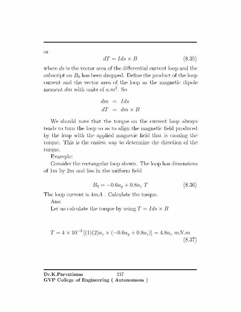
ordT = Ids×B (8.35)
where ds is the vector area of the di�erential current loop and thesubscript on B0 has been dropped. De�ne the product of the loopcurrent and the vector area of the loop as the magnetic dipolemoment dm with units of a.m2. So
dm = Ids
dT = dm×B
We should note that the torque on the current loop alwaystends to turn the loop so as to align the magnetic �eld producedby the loop with the applied magnetic �eld that is causing thetorque. This is the easiest way to determine the direction of thetorque.
Example:Consider the rectangular loop shown. The loop has dimensions
of 1m by 2m and lies in the uniform �eld
B0 = −0.6ay + 0.8az T (8.36)
The loop current is 4mA . Calculate the torque.Ans:Let us calculate the torque by using T = Ids×B
T = 4× 10⁻³ [(1)(2)az × (−0.6ay + 0.8az)] = 4.8ax mN.m(8.37)
Dr.K.ParvatisamGVP College of Engineering ( Autonomous )
237
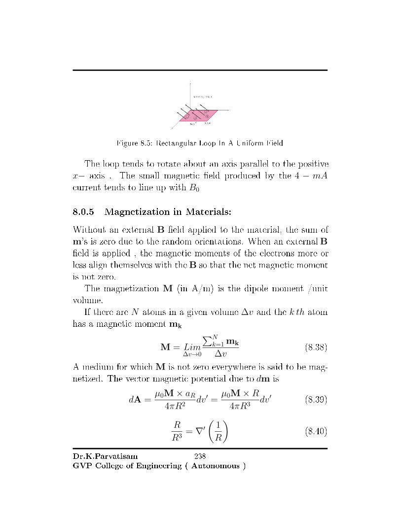
Figure 8.5: Rectangular Loop In A Uniform Field
The loop tends to rotate about an axis parallel to the positivex− axis . The small magnetic �eld produced by the 4 − mA
current tends to line up with B0
8.0.5 Magnetization in Materials:
Without an external B �eld applied to the material, the sum ofm's is zero due to the random orientations. When an externalB�eld is applied , the magnetic moments of the electrons more orless align themselves with theB so that the net magnetic momentis not zero.
The magnetization M (in A/m) is the dipole moment /unitvolume.
If there are N atoms in a given volume ∆v and the k th atomhas a magnetic moment mk
M = Lim∆v→0
∑Nk=1 mk
∆v(8.38)
A medium for which M is not zero everywhere is said to be mag-netized. The vector magnetic potential due to dm is
dA =µ0M× aR
4πR2dv′ =
µ0M×R4πR3
dv′ (8.39)
R
R3= ∇′
(1
R
)(8.40)
Dr.K.ParvatisamGVP College of Engineering ( Autonomous )
238

Hence
A =µ0
4π
ˆM×∇′
(1
R
)dv′ (8.41)
M×∇′(
1
R
)=
(1
R
)∇′ ×M−∇′ ×
(M
R
)(8.42)
So
A =µ0
4π
ˆ
v′
(1
R
)∇′ ×Mdv′ − µ0
4π
ˆ
v′
∇′ ×M
Rdv′ (8.43)
From the vector identityˆ
v′
∇′ × Fdv′ = −˛
s′
F× ds (8.44)
we can rewrite the expression for A as
A =µ0
4π
ˆv′
∇′ ×M
Rdv′ +
˛
s′
M× anR
ds′
=µ0
4π
ˆv′
Jb
Rdv′ +
˛
s′
Kb
Rds′
Jb =∇×M Kb = M×an
where Jb = Bound current density andKb = Bound surface current density. In free space M = 0 and we have
∇×H = Jf (8.45)
or
∇× B
µ0= Jf (8.46)
Dr.K.ParvatisamGVP College of Engineering ( Autonomous )
239

where Jf is the free volume current density. In material mediumM 6= 0 , and as a result B changes
∇× B
µ0=Jf + Jb = J
=∇×H +∇×M
orB = µ0 (H + M) (8.47)
butM =χmH, B = µ0 (1 + χm)H = µ0µrH (8.48)
µr = 1 + χm =µ
µ0(8.49)
µ = µ0µr and is called the permeability of the material.
8.0.6 Magnetic Boundary Conditions:
Figure below shows a boundary between two isotropic materialswith permeabilities µ1 and µ2 . The boundary condition on thenormal components is determined by allowing the surface to cutsmall cylindrical Gaussian surface.
Dr.K.ParvatisamGVP College of Engineering ( Autonomous )
240

Magnetic Boundary Conditions
Applying Gauss law for the magnetic �eld˛
s
B•ds = 0 (8.50)
we �nd thatBN14s−BN24s = 0 (8.51)
or
BN1 = BN2 (8.52)
ThusHN2 =
µ1
µ2HN1 (8.53)
The normal component of B is continuous , but the normal com-ponent of H is discontinuous by the ratio µ1
µ2. The relationship
between the normal components ofM , of course is �xed once therelationship between the normal components ofH is known. Theresult is
MN2 =χm2µ1
χm1µ2(8.54)
Next, apply Amper's circuital law to the rectangular loop˛H•dl = I (8.55)
Taking a clockwise trip along the loop we �n that
Ht14l −Ht24l = K4l (8.56)
where we assume that the boundary may carry a currentK whosecomponent normal to the plane of the closed path isK. Thus
(8.57)
Dr.K.ParvatisamGVP College of Engineering ( Autonomous )
241

Unit-VII
Magnetic Potential:
Scalar Magnetic potential and its limitations � vector mag-netic potential and its properties � vector magnetic potential dueto simple con�gurations � vector Poisson's equations. Self andMutual inductance � Neumans's formulae � determination of self-inductance of a solenoid and toroid and mutual inductance be-tween a straight long wire and a square loop wire in the sameplane � energy stored and density in a magnetic �eld. Introduc-tion to permanent magnets, their characteristics and applications.

Chapter 9
Magnetic potential
Joseph Henry (December 17, 1797 �May 13, 1878) was an American scien-tist who served as the �rst Secretary ofthe Smithsonian Institution, as well as afounding member of the National Insti-tute for the Promotion of Science, a pre-cursor of the Smithsonian Institution.[1]During his lifetime, he was highly re-garded. While building electromagnets,Henry discovered the electromagneticphenomenon of self-inductance. He alsodiscovered mutual inductance indepen-dently of Michael Faraday, though Fara-day was the �rst to publish his results.[2][3] Henry was the inventorof the electric doorbell (1831)[4] and relay (1835).[5] The SI unitof inductance, the henry, is named in his honor. Henry's work onthe electromagnetic relay was the basis of the electrical telegraph,invented by Samuel Morse and Charles Wheatstone separately.
243

9.1. SCALAR MAGNETIC POTENTIAL:
9.1 Scalar magnetic potential:
In electrostatics ,∇×E = 0 . So E is expressed as−∇V , where Vis a scalar potential. This is a stepping stone which allows solvingproblems using several small steps.
In magnetic �elds , H can also be expressed as a gradient of ascalar magnetic potential . So
H = −∇Vm (9.1)
The selection of −ve gradient will provide us with a clear analogyto the electrical potential. The above de�nition should not con�ictwith our previous results
∇×H = J = ∇× (−∇Vm) (9.2)
but curlgrad of any scalar is zero(vector identity). So ifH is to bede�ned as the gradient of a scalar , then current density must bezero throughout the region in which the scalar magnetic potentialis so de�ned.
H = −∇Vm (J = 0) (9.3)
Many magnetic problems involve geometries in which the currentcarrying conductors occupy a relatively small fraction of the totalregion of interest. The dimensions of Vm are Ampere.
In free space
∇ •B =µ0∇ •H = 0
µ0∇ • (−∇Vm) =0
∇2Vm =0 (J = 0)
Unlike electrostatic potential Vm is not a single valued function ofposition.Example:
Consider the cross section of the co-axial line shown.
Dr.K.ParvatisamGVP College of Engineering ( Autonomous )
244
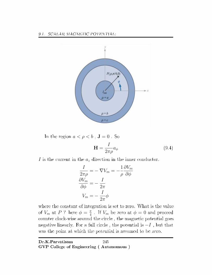
9.1. SCALAR MAGNETIC POTENTIAL:
In the region a < ρ < b , J = 0 . So
H =I
2πρaφ (9.4)
I is the current in the az direction in the inner conductor.
I
2πρ=−∇Vm = −1
ρ
∂Vm∂φ
∂Vm∂φ
=− I
2π
Vm =− I
2πφ
where the constant of integration is set to zero. What is the valueof Vm at P ? here φ = π
4 . If Vm be zero at φ = 0 and proceedcounter clock-wise around the circle , the magnetic potential goesnegative linearly. For a full circle , the potential is −I , but thatwas the point at which the potential is assumed to be zero.
Dr.K.ParvatisamGVP College of Engineering ( Autonomous )
245

9.1. SCALAR MAGNETIC POTENTIAL:
At P, φ = π4 ,
9π4 ,
17π4 or − 7π
4 ,−23π4 .....etc
VmP =I
2π
(2n− 1
4
)π, (n = 0,±1,±2, .....) (9.5)
The reason for this is
∇× E =0˛
l
E • dl =0
Vmab =−aˆ
b
H • dl (where a speci�c path is to be selected )
Magnetic scalar potential is not a conservative �eld.
9.1.1 Vector Magnetic Potential:
we know that for a magnetic �eld
∇ •B = 0 (9.6)
From the vector identity
∇ • (∇×A) = 0 (9.7)
So if the divergence of a vector �eld is zero, then this vector canbe expressed as the curl of another vector. As the divergenceof the magnetic �ux density is always zero, the vector B can beexpressed as the curl of another vector. That is
B = ∇×A (9.8)
This can always be done for a divergence free (solenoidal) �eld .The vector A is called the vector magnetic potential .
It is important to note the following:
Dr.K.ParvatisamGVP College of Engineering ( Autonomous )
246

9.1. SCALAR MAGNETIC POTENTIAL:
1. The magnetic vector potential is de�ned based on the diver-gence free condition of B .
2. The de�nition of A is entirely based on the mathematicalproperties of the vector B , not on its physical characteris-tics . In this sense , A is viewed as an auxiliary functionrather than a fundamental �eld quantity. Nevertheless, themagnetic vector potential is an important function with con-siderable utility. we will make considerable use of the mag-netic vector potential .
3. Since the magnetic vector potential is a vector quantity ,both its curl and divergence must be speci�ed. The curl isspeci�ed by the above equation. We can safely assume thatthe divergence is zero (∇ •A = 0) .
4. The magnetic vector potential does not have a simple physi-cal meaning in the sense that it is not a measurable physicalquantity like B or H . It may seem a bit unsettling to de�nea physical quantity based on the mathematical properties ofanother function and then use this secondary function to eval-uate physical properties of the magnetic �eld. In fact there isnothing unusual about this process. We can view the de�ni-tion of the magnetic vector potential as a transformation. Aslong as the inverse transformation is unique , there is nothingwrong in A not having a readily de�ned physical meaning.We can use the magnetic vector potential in any way that isconsistent with the properties of a vector �eld and the rulesof vector algebra. If we then transform back to the magnetic�ux density using the equation B = ∇×A , all results thusobtained are correct.
Dr.K.ParvatisamGVP College of Engineering ( Autonomous )
247

9.1. SCALAR MAGNETIC POTENTIAL:
5. because the magnetic vector potential relates to the magnetic�ux density through the curl , the magnetic vector potentialA is at right angles to the magnetic �ux densityB .
6. The units of A are wb/m .
Now we want to get an expression forA .
B2 = ∇2 ×A2 =µ0
4π
˛I1dl1 × aR12
R212
= −µ0
4π
˛aR12× I1dl1R2
12
but − aR12
R212
=∇2
(1
R12
)so B2 = ∇2 ×A2 =
µ0
4π
˛∇2
(1
R12
)× I1dl1
to this add1
R12(∇2 × I1dl1) =0
B2 = ∇2 ×A2 =µ0
4π
[˛∇2
(1
R12
)× I1dl1 +
˛1
R12(∇2 × I1dl1)
]from the identity
˛∇2 ×
(I1dl1R12
)=
[˛∇2
(1
R12
)× I1dl1 +
˛1
R12(∇2 × I1dl1)
]we can write B2 = ∇2 ×A2 =
µ0
4π
˛∇2 ×
(I1dl1R12
)=
˛∇2 ×
(µ0
4π
I1dl1R12
)B2 = ∇2 ×A2 =∇2 ×
˛ (µ0
4π
I1dl1R12
)A2 =
µ0
4π
˛I1dl1R12
The signi�cance of the terms in the above equation is the sameas in the Biot-Savart law : a direct current I �ows along a �la-mentary conductor of which any di�erential length dL is distantR from the point at whichA is to be found. Since we have de�nedA only through speci�cation of its curl , it is possible to add the
Dr.K.ParvatisamGVP College of Engineering ( Autonomous )
248

9.1. SCALAR MAGNETIC POTENTIAL:
gradient of any scalar �eld to the equation forA without chang-ing B or H, for the the curl of the gradient is identically zero. Insteady magnetic �elds , it is customary to set this possible addedterm equal to zero.
Dr.K.ParvatisamGVP College of Engineering ( Autonomous )
249

Unit-VIII
Time varying �elds :
Time varying �elds � Faraday's laws of electromagnetic induc-tion � Its integral and point forms � Maxwell's fourth equation,∇×E = −∂B
∂t � Statically and Dynamically induced EMFs � Simpleproblems. Modi�cation of Maxwell's equations for time varying�elds � Displacement current � Poynting Theorem and

251

Chapter 10
FARADAY'S LAW AND
ELECTROMAGNETIC
INDUCTION
Michael Faraday, FRS (22 September1791 � 25 August 1867) was an En-glish scientist who contributed to the�elds of electromagnetism and electro-chemistry. His main discoveries includethat of electromagnetic induction, dia-magnetism and electrolysis.Although Faraday received little formaleducation he was one of the most in�u-ential scientists in history,[1] and histo-rians of science[2] refer to him as havingbeen the best experimentalist in the his-tory of science.[3] It was by his researchon the magnetic �eld around a conductor carrying a direct cur-rent that Faraday established the basis for the concept of the elec-tromagnetic �eld in physics. Faraday also established that mag-netism could a�ect rays of light and that there was an underlyingrelationship between the two phenomena.[4][5] He similarly dis-covered the principle of electromagnetic induction, diamagnetism,and the laws of electrolysis. His inventions of electromagnetic ro-tary devices formed the foundation of electric motor technology,and it was largely due to his e�orts that electricity became viablefor use in technology.
Dr.K.ParvatisamGVP College of Engineering ( Autonomous )
252

Heinrich Friedrich Emil Lenz (12 Febru-ary 1804 � 10 February 1865) was a Rus-sian physicist of Baltic German ethnic-ity. He is most noted for formulatingLenz's law in electrodynamics in 1833.The symbol L, conventionally represent-ing inductance, is chosen in his honor.[1]Lenz was born in Dorpat (now Tartu,Estonia), the Governorate of Livonia, inthe Russian Empire at that time. Aftercompleting his secondary education in 1820, Lenz studied chem-istry and physics at the University of Dorpat. He traveled with thenavigator Otto von Kotzebue on his third expedition around theworld from 1823 to 1826. On the voyage Lenz studied climaticconditions and the physical properties of seawater. The resultshave been published in "Memoirs of the St. Petersburg Academyof Sciences" (1831).After the voyage, Lenz began working at the University of St.Petersburg, Russia, where he later served as the Dean of Mathe-matics and Physics from 1840 to 1863 and was Rector from 1863until his death in 1865. Lenz also taught at the Petrischule in1830 and 1831, and at the Mikhailovskaya Artillery Academy.Lenz had begun studying electromagnetism in 1831. Besidesthe law named in his honor, Lenz also independently discoveredJoule's law in 1842; to honor his e�orts on the problem, it isalso given the name the "Joule�Lenz law," named also for JamesPrescott Joule.
When static conditions hold ie when time does not enter intothe picture, electricity and magnetism are two separate , some-what parallel disciplines. This can be seen by observing that
Dr.K.ParvatisamGVP College of Engineering ( Autonomous )
253

Maxwell's equations, appear as two sets of equations which areindependent of each other ie the two equations describing the elec-tric �eld has no term which contains a magnetic quantity and thetwo equations which describe the magnetic �eld do not containany electrical �eld quantity.
∇ • E =ρ
ε0,∇ •B = 0
∇× E = 0,∇×B = µ0J
Expressed in terms of the potential �elds, these equations areequivalent to
φ =1
4πε0
ˆ
v
ρ
Rdτ, A =
µ0
4π
ˆ
v
J
Rdv
ρ is the cause, φ and E are the results. J is the cause, A and Bare the results. The forces are assumed to be transmitted eitherwith in�nite speed or with �nite speed such that su�cient time isallowed for an equilibrium situation to develop.
If time varying �elds are considered, the equations∇ • E and∇•B remain the same but the other two equations require mod-i�cation.
When conditions are changing only slowly with respect to time,it is called quasi-static. When conditions are changing rapidly, itis called time varying (radiation e�ects).
1820 Oerstead demonstrated that an electric current a�ects acompass needle. In 1831 Faraday showed that a time changingmagnetic �eld will produce an electromotive force.
e.m.f = −dφdt
(10.1)
The change in �ux may result from
Dr.K.ParvatisamGVP College of Engineering ( Autonomous )
254

• A time changing �ux linking a stationary path
• Relative motion between �ux and a closed path
• Combination of the above two
The �rst one is called the transformer e.m.f. The second one iscalled motional e.m.f.
Consider an arrangement of a conducting loop with a gal-vanometer in the loop and either a permanent magnet or a currentcarrying coil placed near the conducting loop. Considering vari-ous situations the following observations can be made.
1 Place a magnet near theconducting loop
No current �owsthrough thegalvanometer
2 Move the magnettowards the loop
The gal-vanometerregisters acurrent
3 Reverse thedirection ofmotion of themagnet
The gal-vanometerde�ectionreverses
4 Reverse the polarity of themagnet and move themagnet
The galvanometerde�ection reverses
Dr.K.ParvatisamGVP College of Engineering ( Autonomous )
255

5 Keep the magnet �xedand move the coiltowards the magnet
The gal-vanometerregisters acurrent
6 Increase thespeed of themagnet
Thede�ectionincreases
7 Increase thestrength of themagnet
The de�ection increases
8 Increase thediameter of thecoil
The de�ection increases
9 Fix the speed of the magnet butrepeat with the magnet closer to thecoil
The de�ection of the galvanometerincreases
10 Move the magnetat an angle to thecoil
The gal-vanometerde�ectiondecreases
Dr.K.ParvatisamGVP College of Engineering ( Autonomous )
256

11 Increase thenumber of turnsof the coil
Magnitudeof thecurrentincreases
10.0.1 Transformer e.m.f:
If a closed stationary path in space which is linked with a changingmagnetic �eld is considered, it is found that the induced voltagearound this path is equal to the negative rate of change of thetotal �ux through the path.˛
E • dl = vind (10.2)
but
vind = −∂φ∂t
= − ∂∂t
ˆ
s
B • ds (10.3)
which results in ˛E • dl = − ∂
∂t
ˆ
s
B • ds (10.4)
the �gures of our right hand indicate the direction of closedpath, and our thumb indicates the direction of ds . A �ux densityB , in the direction of ds and increasing with time, thus producesan average value of E which is opposite to the positive directionabout the closed path. The rigt handed relationship between thesurface integral and the closed line integral should always be kept
Dr.K.ParvatisamGVP College of Engineering ( Autonomous )
257
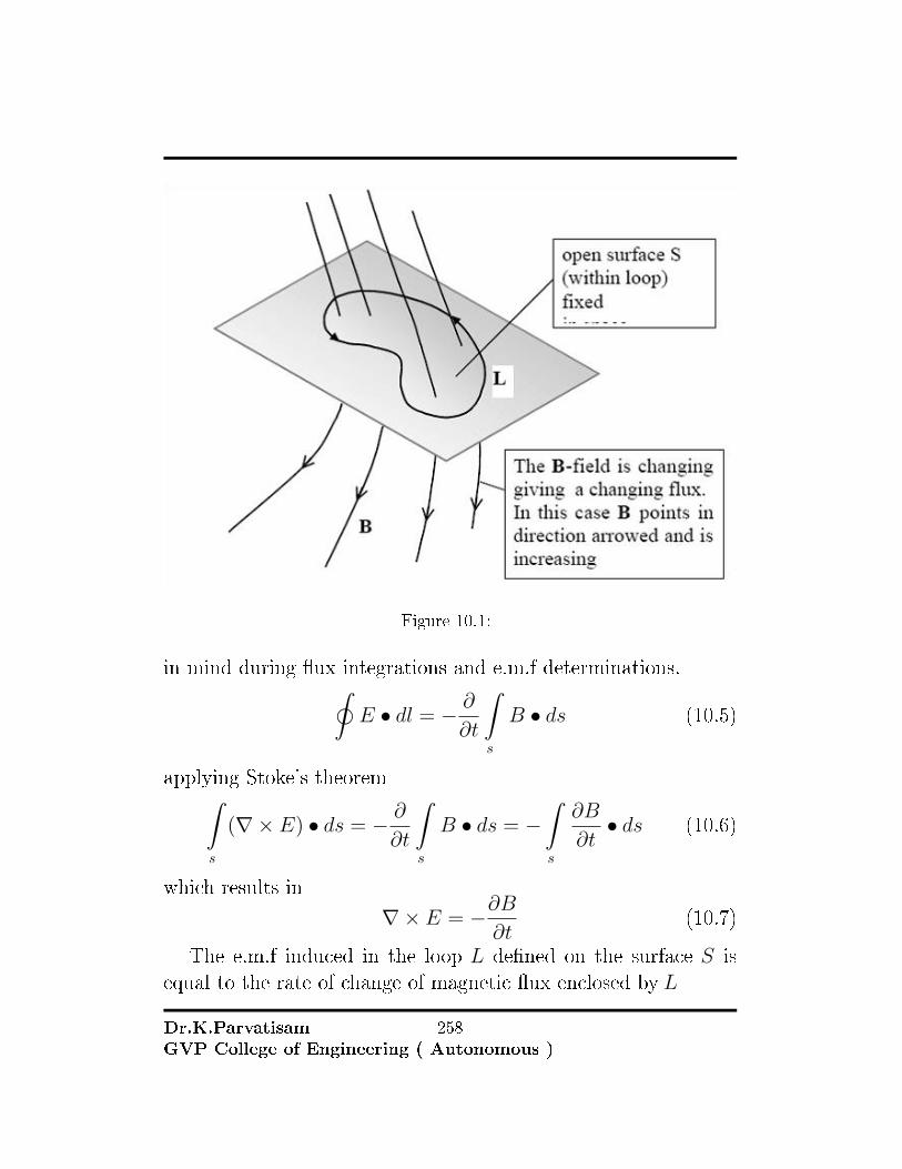
Figure 10.1:
in mind during �ux integrations and e.m.f determinations.˛E • dl = − ∂
∂t
ˆ
s
B • ds (10.5)
applying Stoke's theoremˆ
s
(∇× E) • ds = − ∂∂t
ˆ
s
B • ds = −ˆ
s
∂B
∂t• ds (10.6)
which results in
∇× E = −∂B∂t
(10.7)
The e.m.f induced in the loop L de�ned on the surface S isequal to the rate of change of magnetic �ux enclosed by L
Dr.K.ParvatisamGVP College of Engineering ( Autonomous )
258

Figure 10.2:
The �gure below shows the case of e.m.f induced when a per-manent magnet is moved into a loop of wire
10.0.2 Motional e.m.f:
please refer to the �gure given below. The magnetic �ux densityB is costant (in space and in time) and is normal to the planecontaining the closed path.
Let the shorting bar be moving with a velocity v m/s. Let thebar move a small distance dl in time dt. then dl = vdt. Then thedi�erential �ux change is given by dφ = BvLdt. The magnitudeof the e.m.f induced is equal to
vind = −dφdt
= −BLv (10.8)
In the general case where the direction of the movement of theconductor and the direction of the �ux is such that they are not
Dr.K.ParvatisamGVP College of Engineering ( Autonomous )
259
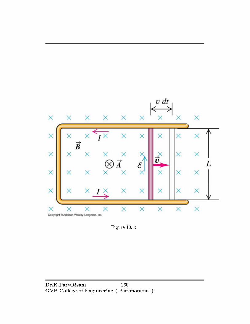
Figure 10.3:
Dr.K.ParvatisamGVP College of Engineering ( Autonomous )
260

orthogonal to each other then the emf induced is given in bothmagnitude and direction by
vind =
˛(v ×B) • dl (10.9)
Lenz's Law: The polarity of th induced e.m.f is given by Lenz'slaw. The Lenz's law states that the induced voltage acts to pro-duce a �ux which will try to oppose the original �ux change whichis the cause of production of the e.m.f. Th e following �gures showthe application of Lenz's law under various situations.
Figure 10.4:
The �gure below shows di�erent situations and the applicationof the Lenz's law
Dr.K.ParvatisamGVP College of Engineering ( Autonomous )
261

Figure 10.5:
The �gure below is another way of looking at Lenz's law
Dr.K.ParvatisamGVP College of Engineering ( Autonomous )
262

Figure 10.6: Di�erent Situations And The E.M.F Induced
10.0.3 Displacement Current density:
Faraday's law as one of Maxwell's equation in di�erential form isgiven by
∇× E = −∂B∂t
which shows that time cahanging magnetic �eld produces an elec-tric �eld. This electric �eld has the special property that its lineintegral around a closed path is not zero. let us see what happens
Dr.K.ParvatisamGVP College of Engineering ( Autonomous )
263
when a time changing electric �eld is considered. Consider thepoint form of the Ampere's circuital law
∇×H = J and see what happens when we take the divergence∇•∇×H = 0 = ∇•J(10.10)
Since the divergence of curl is identically zero∇• J = 0 Howeverthe equation of continuity shows that it can be true only if
∂ρv∂t
= 0 (10.11)
This is an unrealistic limitation and the formula∇×H = J mustbe ammended .
Suppose we add an unknown term G to ∇×H = J , then theequation becomes
∇×H = J +G (10.12)
Again taking the divergence we have
0 = ∇ • J +∇ •G (10.13)
Thus
∇ •G =∂ρv∂t
(10.14)
Replacing ρv by ∇ •D
∇ •G =∂
∂t(∇ •D) = ∇ • ∂D
∂t(10.15)
from which we obtain for G as
G =∂D
∂t(10.16)
Ampere's circuital law in point from then becomes
Dr.K.ParvatisamGVP College of Engineering ( Autonomous )
264

∇×H = J +∂D
∂t(10.17)
The above equation is not derived. It is merely a form that wasobtained which does not disagree with the continuity equation. Itis also consistent all other results. The additional term ∂D
∂t hasthe dimensions of current density , Amp/square meter. Since itresults from a time varying electrical �ux density ( or displacementdensity), this is called as displacement current density . It issometimes denoted by Jd
∇×H = J + Jd
Jd =∂D
∂t
we have encountered three types of current density they areConduction current density
J = σE (10.18)
Convection current density
J = ρvv (10.19)
Displacement current density
Jd =∂D
∂t(10.20)
The total displacement current crossing any given surface isexpressed by the surface integral
Id =
ˆ
s
Jd • ds =
ˆ
s
∂D
∂t• ds (10.21)
Dr.K.ParvatisamGVP College of Engineering ( Autonomous )
265

and this leads to the time-vaying version of the Ampere's circuitallawˆ
s
(∇×H) • ds =
ˆ
s
J • ds+
ˆ
s
Jd • ds =
ˆ
s
J • ds+
ˆ
s
∂D
∂t• ds
(10.22)and applying Stoke's theorem
˛H•dl = I+Id = I+
ˆ
s
∂D
∂t•ds
(10.23)
What is the nature of displacement current density? Let usstudy the simple circuit shown in the �gure.
Figure 10.7: Filamentary Conducting Loop In A Time-varying MagneticField
Dr.K.ParvatisamGVP College of Engineering ( Autonomous )
266

It contains a �lamentary loop and a parallel plate capacitor.With the loop a magnetic �eld varying sinusoidally with time isapplied to produce an e.m.f about the closed path (the �lamentplus the dashed portion between the capacitor plates) which weshall take as
e.m.f = V0 cosωt (10.24)
Using elementary circuit theory concepts and assuming that theloop has negligible resistance and inductance, we may obtain thecurrent in the loop as
I = −ωCV0 cosωt
I = −ωεSd
sinωt
where the quantities ε, S, d pertain to the capacitor. Let us applyAmpere's circuital law about the smaller closed circular path kand neglect the displacement current for the moment
˛
k
H • dl = Ik (10.25)
The path and the value of H along the path are both de�nitequantities ( although di�cult to determine), and
¸kH • dl is a
de�nite quantity. The current Ik is that current through everysurface whose perimeter is the path k . If we choose a simplesurface punctured by the �lament , such as the plane circular sur-face de�ned by the circular path k , the current is evidently theconduction current . Suppose now we consider the closed path kas the mouth of a paper bag whose bottom passes between thecapacitor plates. The bag is not pierced by the �lament, and the
Dr.K.ParvatisamGVP College of Engineering ( Autonomous )
267

conduction current is zero. Now we need to consider the displace-ment current, for within the capacitor
D = εE = ε
(V0
dcosωt
)(10.26)
and thereforeId = −ωεs
dV0 sinωt (10.27)
This is the same value as that of the conduction current in the�lamentary loop. The application of the Ampere's circuital lawincluding the displacement current to the pathk leads to a de�nitevalue for the line integral of H . This value must be equal to thetotal current crossing the chosen surface . For some surfaces thecurrent is almost entirely conduction current, but for those sur-faces passing between the capacitor plates, the conduction currentis zero , and it is the displacement current which is now equal tothe closed line integral of H .
Displacement current is associated with time varying electric�elds and therefore exists in all imperfect conductors carryingtime-varying conduction current. The reason why this additionalcurrent was never discovered experimentally is, it is very verysmall compared to the conduction current.
Dr.K.ParvatisamGVP College of Engineering ( Autonomous )
268

Maxwell's Equations
Static Fields
Pointor
Di�erential FormIntegral Form
'
&
$
%
∇ •D = ρv
∇× E = 0
∇ •B = 0
∇×H = Jc
'
&
$
%
˛
s
D • ds =
ˆ
v
ρvdv
˛
l
E • dl = 0
˛
s
B • ds = 0
˛
l
H • dl =
˛
s
Jc • ds
Dr.K.ParvatisamGVP College of Engineering ( Autonomous )
269
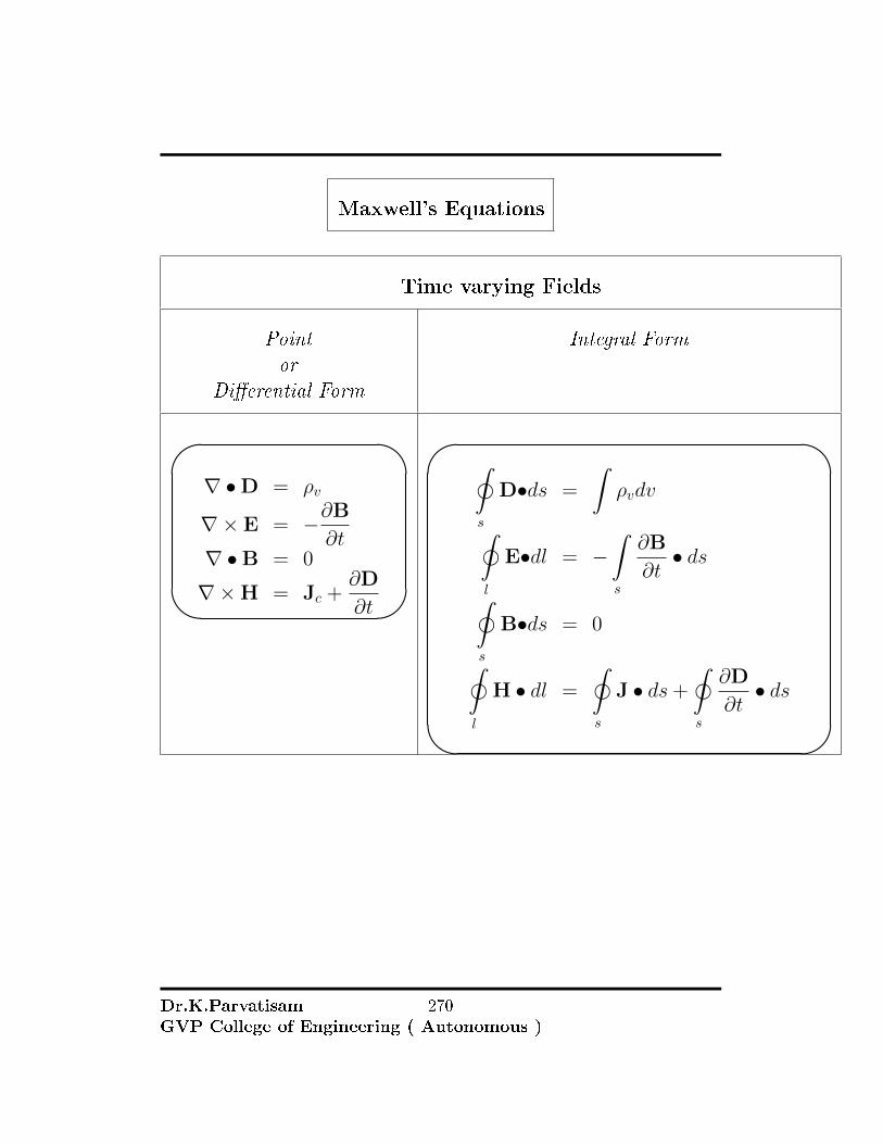
Maxwell's Equations
Time varying Fields
Pointor
Di�erential Form
Integral Form
'
&
$
%
∇ •D = ρv
∇× E = −∂B∂t
∇ •B = 0
∇×H = Jc +∂D
∂t
'
&
$
%
˛
s
D•ds =
ˆρvdv
˛
l
E•dl = −ˆ
s
∂B
∂t• ds
˛
s
B•ds = 0
˛
l
H • dl =
˛
s
J • ds+
˛
s
∂D
∂t• ds
Dr.K.ParvatisamGVP College of Engineering ( Autonomous )
270
Maxwell's equations represent mathematical expressions of cer-tain experimental results. In this light it is apparent that theycannot be proved; however , the applicability to any situation canbe veri�ed. As a result of extensive experimental work, Maxwell'sequations are now believed to apply to all macroscopic situation-sand they are used, much like conservation of momentum, as guid-ing principles. They are the fundamental equations of the elec-tromagnetic �elds produced by the source charges and currentdensities ρ and J . If the material bodies are present , in order touse the Maxwell's equations, one must also know the applicableconstitutive equations - either experimentally or from a micro-scopic theory of the particular kind of matter; D = D(E) andH = H(B)
Maxwell's integral laws encompass the laws of electrical cir-cuits. The transition from �elds to circuits is made by associat-ing the relevant volumes, surfaces, and contours with electrodes,wires, and terminal pairs. Begun in an informal way in Chap. 1,this use of the integral laws will be formalized and examined asthe following chapters unfold. Indeed, many of the empirical ori-gins of the integral laws are in experiments involving electrodes,wires and the like.
The remarkable fact is that the integral laws apply to any com-bination of volume and enclosing surface or surface and enclosingcontour, whether associated with a circuit or not. This was im-plicit in our use of the integral laws for deducing �eld distributionsin Chap. l.
Even though the integral laws can be used to determine the�elds in highly symmetric con�gurations, they are not generallyapplicable to the analysis of realistic problems. Reasons for this liebeyond the geometric complexity of practical systems. Source dis-
Dr.K.ParvatisamGVP College of Engineering ( Autonomous )
271

tributions are not generally known, even when materials are ide-alized as insulators and "perfect" conductors. In actual materials,for example, those having �nite conductivity, the self-consistentinterplay of �elds and sources, must be described.
Because they apply to arbitrary volumes, surfaces, and con-tours, the integral laws also contain the di�erential laws that applyat each point in space. The di�erential laws derived in this chapterprovide a more broadly applicable basis for predicting �elds. Asmight be expected, the point relations must involve informationabout the shape of the �elds in the neighborhood of the point.Thus it is that the integral laws are converted to point relationsby introducing partial derivatives of the �elds with respect to thespatial coordinates.
As a description of the temporal evolution of electromagnetic�elds in three-dimensional space, Maxwell's equations form a con-cise summary of a wider range of phenomena than can be foundin any other discipline. Maxwell's equations are an intellectualachievement that should be familiar to every student of physicalphenomena. As part of the theory of �elds that includes contin-uum mechanics, quantum mechanics, heat and mass transfer, andmany other disciplines, our subject develops the mathematicallanguage and methods that are the basis for these other areas.
To quote Richard Feynman
� From a long view of mankind - seen from, say, ten thousandyears from now - there can be little doubt that the most sig-ni�cant event of the 19 th century will be judged as Maxwell'sdiscovery of the laws of electrodynamics. The American civilwar will pale into insigni�cance in comparison with this im-portant scienti�c event of the same decade�
Dr.K.ParvatisamGVP College of Engineering ( Autonomous )
272

It took the genius of James Clerk Maxwell to unify electricityand magnetism into a super theory, electromagnetism or classicalelectrodynamics (CED), and to realize that optics is a sub-�eldof this new super theory. Early in the 20th century, Nobel lau-reate Hendrik Antoon Lorentz took the electrodynamics theoryfurther to the microscopic scale and also laid the foundation forthe special theory of relativity, formulated by Albert Einstein in1905. In the 1930s Paul A. M. Dirac expanded electrodynamicsto a more symmetric form, including magnetic as well as elec-tric charges and also laid the foundation for the development ofquantum electrodynamics (QED).
Maxwell has made one of the great uni�cations of physics. Be-fore his time, there was light, and there was electricity and mag-netism. The latter two had been uni�ed by the experimental workof Faraday, Oerstead, and ampere. Then, all of a sudden, lightwas no longer � something else,� but was only electricity and mag-netism in the new form - little pieces of electric and magnetic �eldswhich propagate through space on their own.
The �rst equation - that the divergence of E is the chargedensity over ε0 - is true in general. In dynamic as well as in static�elds , Gauss' law is always valid. The �ux ofE through any closedsurface is proportional to the charge inside. The third equation isthe corresponding general law for magnetic �elds. Since there areno magnetic charges, the �ux of B through any closed surface isalways zero. The second equation that the curl of E is −∂B
∂t , isFaraday's law and was discussed . It is also generally true . Thelast equation has something new . We have seen before the partof it which holds for steady currents. In that case we said thatthe curl of B is µ0J , but the correct general expression has a newpart that was discovered by Maxwell.
Dr.K.ParvatisamGVP College of Engineering ( Autonomous )
273

Maxwell's equations are as important today as ever. They ledto the development of special relativity and, nowadays, almostevery optics problem that can be formulated in terms of dielec-tric permittivity and magnetic permeability (two key constantsin Maxwell's equations), ranging from optical �ber waveguidesto meta-materials and transformation optics , is treated withinthe framework of these equations or systems of equations derivedfrom them. Their actual solution can, however, be challenging forall but the most basic physical geometries. Numerical methodsfor solving the equations were pioneered by Kane Yee and AllenTa�ove, but went unnoticed for many years owing to the lim-ited computing power available at the time. Now, however, thesemethods can be easily employed for solving electromagnetic prob-lems for structures as complex as aircraft. By the middle of thenineteenth century, a signi�cant body of experimental and theo-retical knowledge about electricity and magnetism had been accu-mulated. In 1861, James Clerk Maxwell condensed it into 20 equa-tions. Maxwell published various reduced and simpli�ed forms,but Oliver Heaviside is frequently credited with simplifying theminto the modern set of four partial di�erential equations: Fara-day's law, Ampère's law, Gauss' law for magnetism and Gauss'law for electricity. One of the most important contributions madeby Maxwell was actually a correction to Ampère's law. He hadrealized that magnetic �elds can be induced by changing electric�elds � an insight that was not only necessary for accuracy butalso led to a conceptual breakthrough. Maxwell predicted an `elec-tromagnetic wave', which can self-sustain, even in a vacuum, inthe absence of conventional currents. Moreover, he predicted thespeed of this wave to be 310,740,000m/s � within a few percentof the exact value of the speed of light. �The agreement of the
Dr.K.ParvatisamGVP College of Engineering ( Autonomous )
274

results seems to show that light and magnetism are a�ections ofthe same substance, and light is an electromagnetic disturbancepropagated through the �eld according to electromagnetic laws�,wrote Maxwell in 1865. The concept of light was thus uni�ed withelectricity and magnetism for the �rst time.
Dr.K.ParvatisamGVP College of Engineering ( Autonomous )
275

Maxwell's Equations
Static Fields
Pointor
Di�erential FormIntegral Form
'
&
$
%
∇ •D = ρv
∇× E = 0
∇ •B = 0
∇×H = Jc
'
&
$
%
˛
s
D • ds =
ˆ
v
ρvdv
˛
l
E • dl = 0
˛
s
B • ds = 0
˛
l
H • dl =
˛
s
Jc • ds
Dr.K.ParvatisamGVP College of Engineering ( Autonomous )
276

Maxwell's Equations
Time varying Fields
Pointor
Di�erential Form
Integral Form
'
&
$
%
∇ •D = ρv
∇× E = −∂B∂t
∇ •B = 0
∇×H = Jc +∂D
∂t
'
&
$
%
˛
s
D•ds =
ˆρvdv
˛
l
E•dl = −ˆ
s
∂B
∂t• ds
˛
s
B•ds = 0
˛
l
H • dl =
˛
s
J • ds+
˛
s
∂D
∂t• ds
Dr.K.ParvatisamGVP College of Engineering ( Autonomous )
277

Index
E
Electromagnetics, 1
278

Bibliography
[1] L.J.Chu Adler, R.B. and R.M.Fano.
[2] Kuc.R.
[3] Shafer.R.W Oppenhiem.A.v.
279