Embed Size (px)
Citation preview
Modern challenges in stellar population
synthesisJ a r l e B r i n c h m a n n
C A U P

OverviewPopulation synthesis - an overview
The methods & ingredients
Existing models - a brief overview
Challenges as a function of wavelengthThe ionizing flux of hot stars
The UV output of old stars
The optical and non-solar abundance ratios
The TP-AGB contribution in the red.
Some further challenges & a summary
Note: This will focus on UV-NIR stellar populations - see Granato’s lecture for a more holistic view.

Some Buzzwords(Lick) Index: A measure of a feature in a spectrum, typically defined with a central band-pass with two bands around defining the continuum.
Single Stellar Population (SSP): A set of stars all formed at the same time according to a given Initial Mass Function (IMF) and thereafter let to evolve.
Horizontal Branch (HB): The stage in stellar evolution where stars have a helium burning core.
[X/H] = Log X/H - Log (X/H)⦿
α-elements: Elements formed through triple-α reactions, they are copiously produced (relative to iron-peak elements) in core-collapse supernovae.
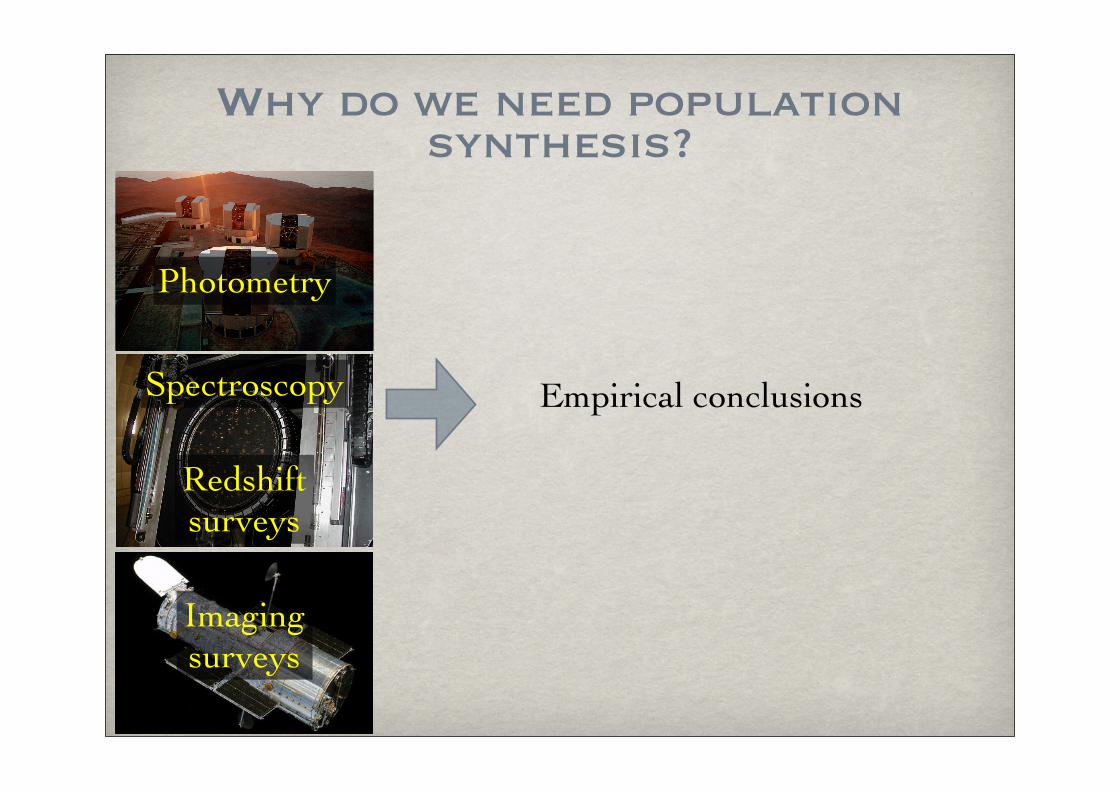
Why do we need population synthesis?
Photometry
Spectroscopy
Redshiftsurveys
Imagingsurveys
Empirical conclusions
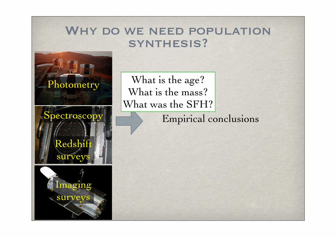
Why do we need population synthesis?
Photometry
Spectroscopy
Redshiftsurveys
Imagingsurveys
What is the age?What is the mass?
What was the SFH?Empirical conclusions
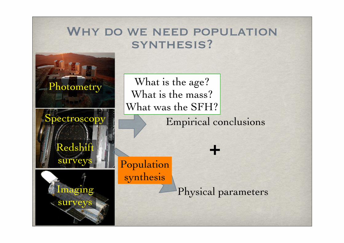
Why do we need population synthesis?
Photometry
Spectroscopy
Redshiftsurveys
Imagingsurveys
What is the age?What is the mass?
What was the SFH?Empirical conclusions
+Populationsynthesis
Physical parameters

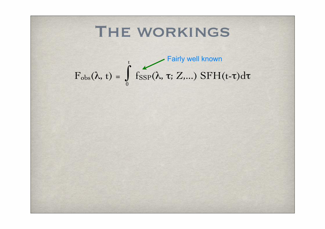
The workings
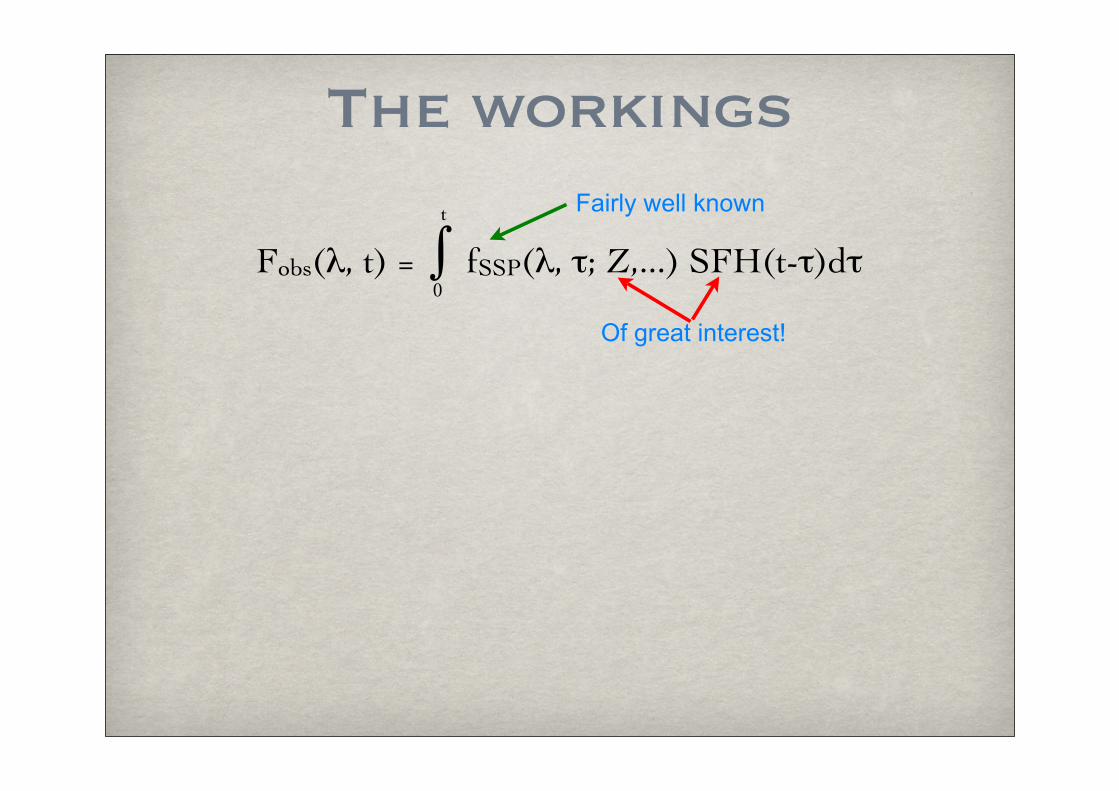
Fobs(λ, t) = ∫ fSSP(λ, τ; Z,...) SFH(t-τ)dτ0
t
The workings
Fobs(λ, t) = ∫ fSSP(λ, τ; Z,...) SFH(t-τ)dτ0
t Fairly well known
The workings
Fobs(λ, t) = ∫ fSSP(λ, τ; Z,...) SFH(t-τ)dτ0
t Fairly well known
Of great interest!

The workings
Fobs(λ, t) = ∫ fSSP(λ, τ; Z,...) SFH(t-τ)dτ0
t Fairly well known
Of great interest!
Requirements for fSSP: Stellar tracks/isochrones (perhaps special treatment for advanced stages) Observed stellar spectra Stellar atmosphere calculations

The workings
Fobs(λ, t) = ∫ fSSP(λ, τ; Z,...) SFH(t-τ)dτ0
t Fairly well known
Of great interest!
Requirements for fSSP: Stellar tracks/isochrones (perhaps special treatment for advanced stages) Observed stellar spectra Stellar atmosphere calculations
The implementation can be done in different ways, e.g. Maraston (1998) vs. Bruzual & Charlot (2003)

Some existing modelsBruzual & Charlot (2003) [BC03] - http://www.cida.ve/~bruzual/bc2003
Very widely used, comes with a set of useful programs to calculate properties. Soon: CB07 using MILES
Starburst 99 - http://www.stsci.edu/science/starburst99/Probably the best treatment of massive stars - more flexibility than in BC03 but more complex as well
Vazdekis’ models - http://www.iac.es/galeria/vazdekis/vazdekis_models.html
The first to produce high resolution SEDs, several improvements but more focused on older stellar populations. New version uses MILES
PÉGASE - http://www2.iap.fr/pegase/General package - previous versions have been low resolution but PÉGASE-HR uses Elodie. Includes chemical evolution directly.
Maraston models - http://www.dsg.port.ac.uk/~marastonc/Extensively tested on GCs - good treatment of TP-AGB & HB.
These are commonly used - but there are are many more!

Stellar evolution - a reminderL
og
L/L
sun
1
2
3
4
3.9 3.63.73.84.0
Log Teff
Sub-Giant branch
RG
B
Core He burning
Core H burning (MS)
Ear
ly A
GB
TP-A
GB
Tracks: Pietrinferni et al (2005)
M=2.5 M⦿Z=0.198Y=0.273
Changes between phases are typically due to changes in where energy is produced.
The exact track followed for a particular star does depend on mass loss, He abundance, whether there are nearby companions, abundance patterns etc. so just specifying Z is not sufficient.
But: Tracks do not provide an emitted spectrum...
Oh, and convective theory: Overshooting?

From tracks to lightAn evolutionary tracks provides the physical & chemical conditions of a star, but to get a spectrum we need another ingredient.

From tracks to lightAn evolutionary tracks provides the physical & chemical conditions of a star, but to get a spectrum we need another ingredient.
Theoretical approach:
abundances, Teff, g F(λ)
Theoretical atmosphere models

From tracks to lightAn evolutionary tracks provides the physical & chemical conditions of a star, but to get a spectrum we need another ingredient.
Theoretical approach:
abundances, Teff, g F(λ)
Theoretical atmosphere models
Semi-empirical approach (best):
abundances, Teff, g
Similar star observed?Yes
NoTheoretical atmosphere
models
Observed spectra
F(λ)
Resolution used to be a concern with models

Resolution used to be a concern with models
Bruzual (2007)
Coelho et al (2007)
IndoUS
MILES
Stelib
HNGSL
Pickles
BaSeL
- no longer
Sampling of Stellar Parameters?
Challenge 1
-3 -2 -1 0 1
0
50
100
[Fe/H]
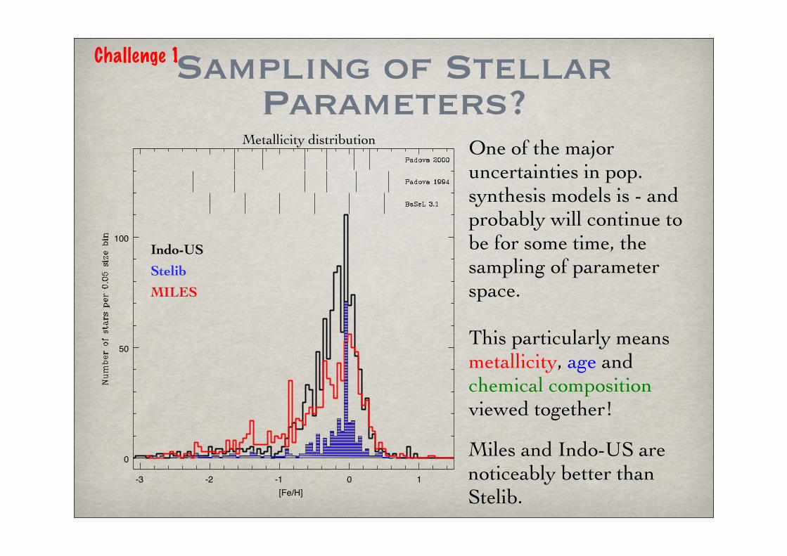
Metallicity distribution
Indo-US
Stelib
MILES
One of the major uncertainties in pop. synthesis models is - and probably will continue to be for some time, the sampling of parameter space.
This particularly means metallicity, age and chemical composition viewed together!
Miles and Indo-US are noticeably better than Stelib.
MS
SGB
RGB
HB
E-AGB
TP-AGB
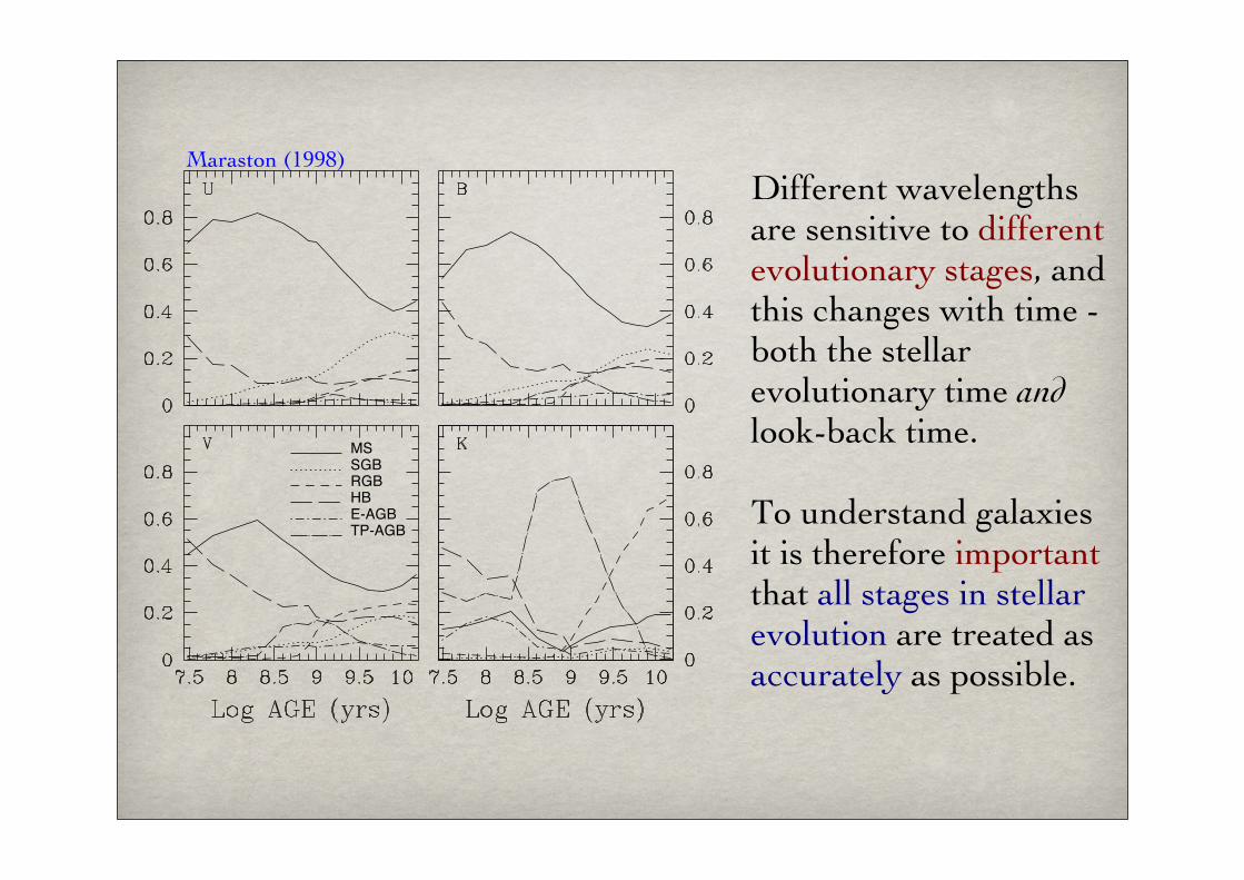
Different wavelengths are sensitive to different evolutionary stages, and this changes with time - both the stellar evolutionary time and look-back time.
To understand galaxies it is therefore important that all stages in stellar evolution are treated as accurately as possible.
Maraston (1998)

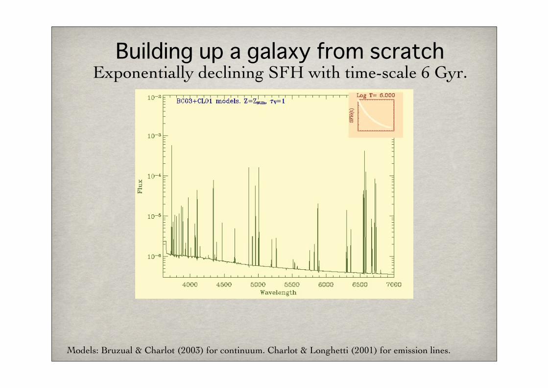
Building up a galaxy from scratchExponentially declining SFH with time-scale 6 Gyr.
Balmer linesModels: Bruzual & Charlot (2003) for continuum. Charlot & Longhetti (2001) for emission lines.
Building up a galaxy from scratchExponentially declining SFH with time-scale 6 Gyr.
Models: Bruzual & Charlot (2003) for continuum. Charlot & Longhetti (2001) for emission lines.

Building up a galaxy from scratchExponentially declining SFH with time-scale 6 Gyr.
D4000 windows
Normalised here

Building up a galaxy from scratchExponentially declining SFH with time-scale 6 Gyr.
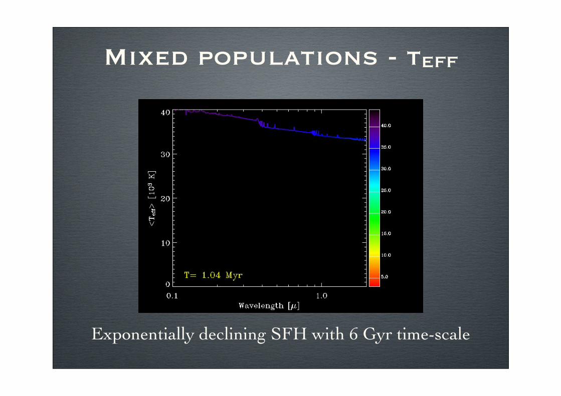
Mixed populations - tEFF
Exponentially declining SFH with 6 Gyr time-scale
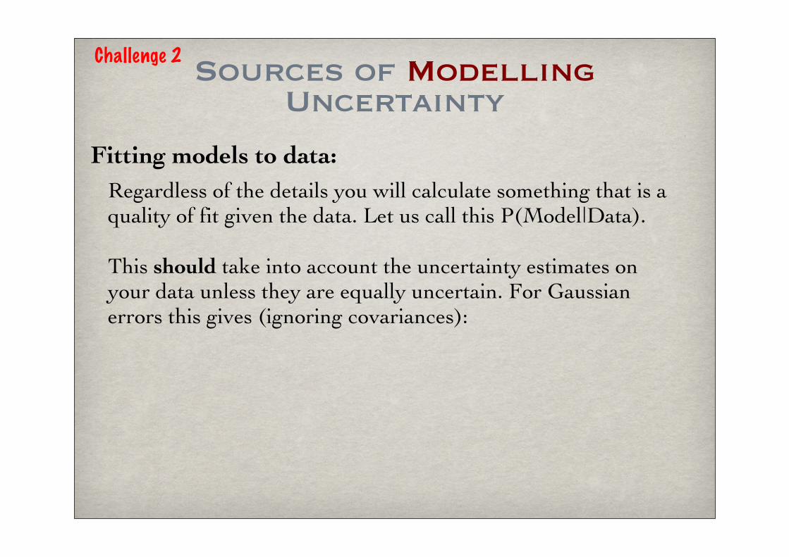
Sources of Modelling Uncertainty
Fitting models to data:Regardless of the details you will calculate something that is a quality of fit given the data. Let us call this P(Model|Data).
This should take into account the uncertainty estimates on your data unless they are equally uncertain. For Gaussian errors this gives (ignoring covariances):
Challenge 2
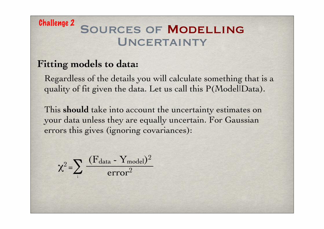
Sources of Modelling Uncertainty
Fitting models to data:Regardless of the details you will calculate something that is a quality of fit given the data. Let us call this P(Model|Data).
This should take into account the uncertainty estimates on your data unless they are equally uncertain. For Gaussian errors this gives (ignoring covariances):
χ2=∑i
(Fdata - Ymodel)2
error2
In the rest of the lecture I’ll talk about this.
So now, let us talk about this.
Challenge 2
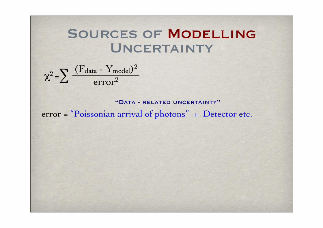
Sources of Modelling Uncertainty
χ2=∑i
(Fdata - Ymodel)2
error2
error = “Poissonian arrival of photons” + Detector etc.“Data - related uncertainty”

Sources of Modelling Uncertainty
χ2=∑i
(Fdata - Ymodel)2
error2
error = “Poissonian arrival of photons” + Detector etc.“Data - related uncertainty”
+ “uncertainty in model predictions”
Normally the data-related uncertainty dominates, but that is not always the case. Without a good uncertainty estimate for data and models you cannot give accurate uncertainty estimates on your derived parameters!

Sources of Modelling Uncertainty
Observational uncertainties in the empirical data (e.g. spectra) included in the models
Uncertainties in atomic data
Mismatch between observed stars and theoretical tracks (e.g. metallicity, age, Teff, log g)
Numerical uncertainties in the model calculation (e.g. interpolation artefacts, numerical precision)
Mismatch between single-parameter model and multi-parameter reality (cf. Kobulnicky, Kennicutt & Pisagno 1999)
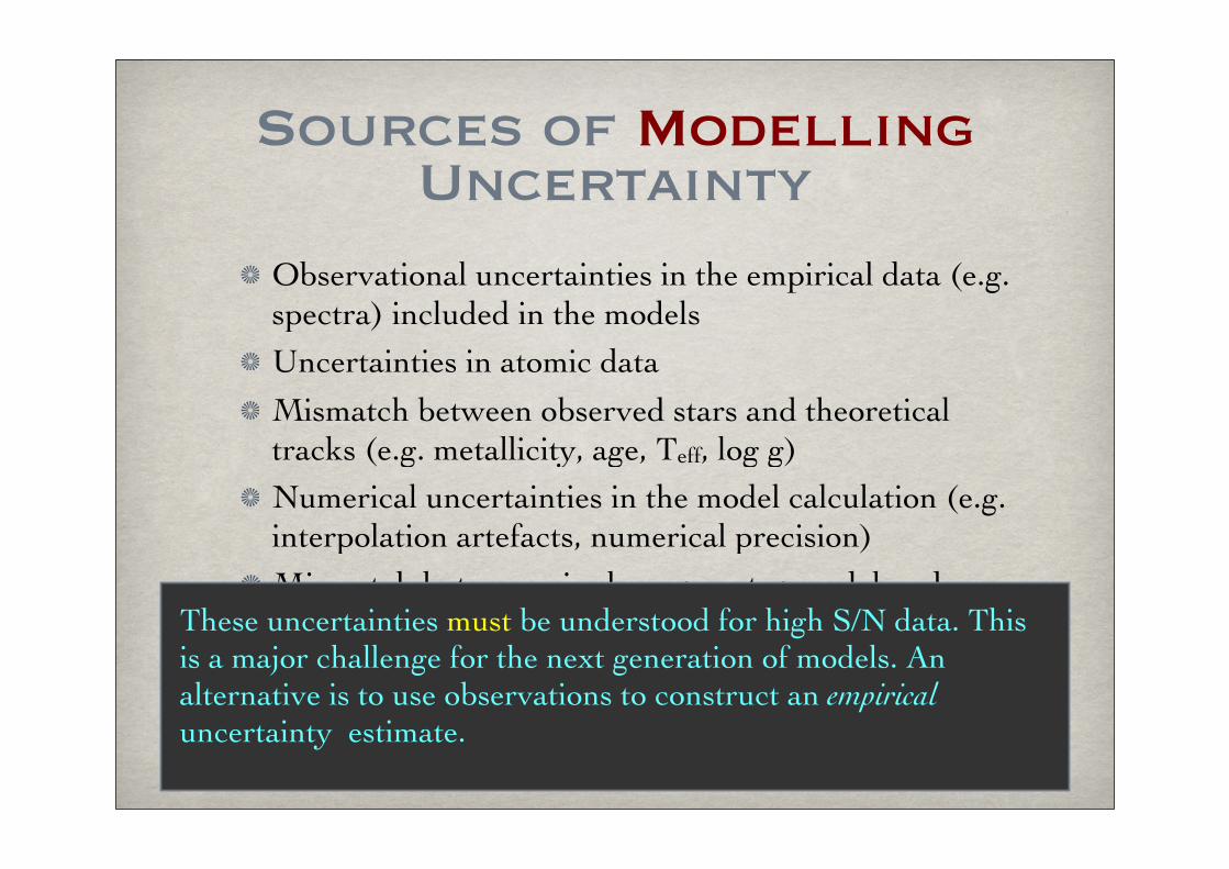
These uncertainties must be understood for high S/N data. This is a major challenge for the next generation of models. An alternative is to use observations to construct an empirical uncertainty estimate.

The Far-UVYoung Massive
Stars

Young stars & outflowsAt λ<1800Å the stellar libraries are fewer and generally with low resolution. Very few direct tests of spectra at λ<912Å.
High redshift observations are typically fairly high resolution - helped by (1+z) stretching.
Young, metal-rich stars are hard to find as are young stars with Z < ZSMC.
This range contains a number of lines that mostly or exclusively originate in the ISM.
Rotation recently realised to be of crucial importance in the evolution of these stars but not yet fully explored (e.g. Meynet & Maeder 2005)
LMC & SMC have Z < Zsun
or in stellar winds
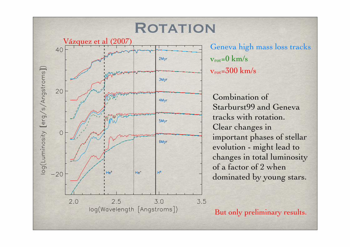
RotationVázquez et al (2007)
Geneva high mass loss tracksvrot=0 km/svrot=300 km/s
Combination of Starburst99 and Geneva tracks with rotation.Clear changes in important phases of stellar evolution - might lead to changes in total luminosity of a factor of 2 when dominated by young stars.
But only preliminary results.

ImportanceIonising Hydrogen
Wolf-Rayet stars
Supernova progenitors
Ionisation of O+, Ne++, He etc.
Constraints on the massive end of the Initial Mass Function.
Constraints on stellar mass-loss at high redshift.
Star formation rate estimators.
Dopita et al (2006)

Does it matter?A short case-study
He II 1640Å
Shapley et al (2003) created a co-added spectrum of Lyman Break Galaxies and found a strong He II 1640Å line.
Brinchmann, Pettini & Charlot (2007)

Does it matter?A short case-study
EW(He II 1640Å) ~ 1.3Å
What causes the strong He II 1640 line in the spectrum of Lyman Break Galaxies? Pop III?
Shapley et al (2003) created a co-added spectrum of Lyman Break Galaxies and found a strong He II 1640Å line.
Brinchmann, Pettini & Charlot (2007)
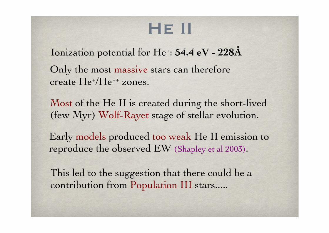
He IIIonization potential for He+: 54.4 eV - 228Å
Only the most massive stars can therefore create He+/He++ zones.
Most of the He II is created during the short-lived (few Myr) Wolf-Rayet stage of stellar evolution.
Early models produced too weak He II emission to reproduce the observed EW (Shapley et al 2003).
This led to the suggestion that there could be a contribution from Population III stars.....

Model ingredients
0.5 1.0 1.5 2.0 2.5 3.0
Log EW (Å)
34.5
35.0
35.5
36.0
36.5
37.0
Log
Lum
inos
ity (
erg
s!1
)
WN3!4WN3!4
WN5!6WN5!6
WN7!9WN7!9
BinariesBinaries
Crowther & Hadfield (2006)
SMC
WR stars in the Milky-Way, LMC & SMC (model atmospheres not yet good enough)
Also:
F(1640)F(4686)
= 10 +/- 1
(Early data gave ~7.9)
+ Add a model for stellar evolution at different metallicities + a Star Formation History

Agreement!
With constant SFH a fixed value is reached and this is in good agreement with the observations.
It might be a useful tool in the future for high-z WR studies.
Constant SFH
The Near-UV Advanced stages of stellar evolution

This wavelength region contains lines from a wide range of chemical elements & lines from energetic winds.
Young starsIn galaxies with on-going star formation, the UV is dominated by young stars.
t=0.5 Gyr
t=8 Gyr
SFH: Exponential with =6 GyrSolar metallicity

This wavelength region contains lines from a wide range of chemical elements & lines from energetic winds.
Young starsIn galaxies with on-going star formation, the UV is dominated by young stars.
t=0.5 Gyr
t=8 Gyr
SFH: Exponential with =6 GyrSolar metallicityVery important spectral range for
high redshift observations:
l=4500Å (B-band) atz=1: 2250Å z=2: 1500Åz=3: 1250Å
So important to improve predictions & integrate with non-stellar processes.

Old (whatever that means) stellar systems do show UV emission: NGC 6681 (Globular cluster)
Blue: Far UV, Green: Near UV, red: optical (Brown et al 2001)
Stars on the MS with Teff<8500K (A5) have very little emission at λ<1800Å (Z~Zsun).
Hotter (younger) stars do however, as do AGN.
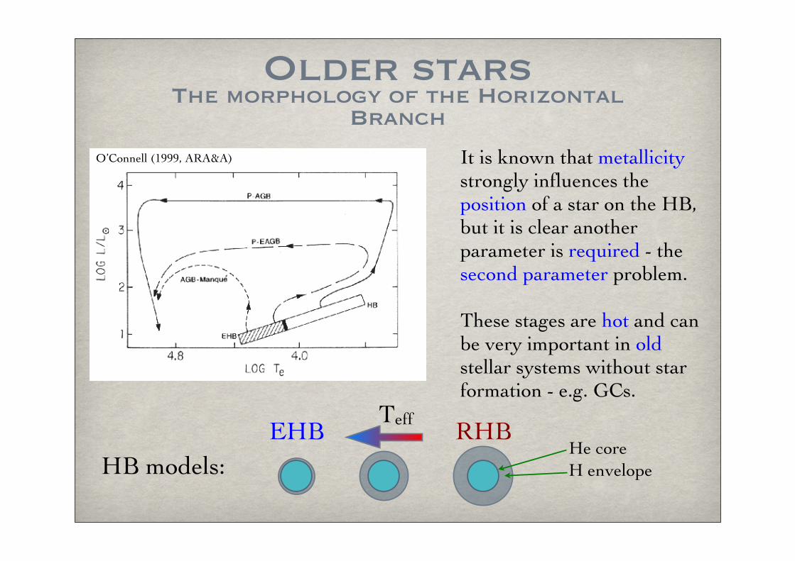
Older starsThe morphology of the Horizontal
Branch
It is known that metallicity strongly influences the position of a star on the HB, but it is clear another parameter is required - the second parameter problem.
These stages are hot and can be very important in old stellar systems without star formation - e.g. GCs.
O’Connell (1999, ARA&A)
EHB RHBHe coreH envelope
Teff
HB models:

The UV-upturn in elliptical galaxies - UVX
Many elliptical galaxies are found to have significant emission in the UV and with significant variation - much more than is seen in the optical.
What is the origin? And can it be used to constrain the properties of the galaxies (Age, Z)?
Large scatter: Additional ingredient needed relative to the optical spectrum.
1500 2000 2500 3000
Wavelength (Å)
16
15
14
13
12
11
10
m
M32
NGC 4649 (-3.0)
O’Donnell (1999, ARA&A)

Status about UVXKnown not to be due to AGN or young population.
The same optical spectrum can give rise to very different FUV properties.
Old He-burning, low mass, stars are most likely.
Extreme Horizontal Branch stars are the most popular candidates. But others have been suggested.
EHB stars are sensitive to details of stellar models so the UVX can either be a good age indicator or a good constraint on stellar models.
Difficult to say how well current models are doing but metallicity & time dependence should be crucial.

Metallicity & the UVXDoes the UVX depend on metallicity?
0.00 0.10 0.20 0.30 0.40 Mg2
5
4
3
2
1
(15
- V) 0
1399
4649
M 32
4382
Galaxies (IUE)Clusters (ANS)Clusters (OAO)
Cen, M 79 (UIT)
M3
47 Tuc
Cen
6388
6441
6752
Rich et al (2005): No.
Burnstein et al (1988): Yes!
Donas et al (2006): Possibly/probably
The metallicity dependence is not clear, but some dependence on Mg2 seems likely.
But is this a metallicity tracer?
Mg2 can vary significantly at constant metallicity.
“UV
X”
Mg2

Look-back time Dependence
Ree et al (2007): Time-dependence of UV upturn for Brightest Cluster Galaxies in Abell clusters is consistent with model predictions.
Main problem with this kind of study: Residual star formation & low-level AGN.
These predictions are based on single-star evolution.

Model predictions - an example
Models: BC03 stochastic library from Salim et al (2005).
The models work well, but the main FUV contribution comes from Post-AGB stars which are not the favoured counter-parts based on direct imaging studies (which prefer EHB stars)
Donas et al (2006)

Model predictionsMain models tailored for the UVX problem:
Metal-poor:
Metal-rich:
Old metal-poor population of hot subdwarfs. Require a substantial spread in metallicity. (Park & Lee 1997)
Metal-rich stars lose most or all of their envelope due to mass loss and requires tuning of mass-loss rate with metallicity (Mg?) as well as high age. (e.g. Yi, Demarque & Oemler 1997)
The problem:
None of these models are very predictive. They require matching to observations (e.g. Maraston et al 2003) and the metal-rich model (which appears to work best) offers no explanation of why mass-loss rates are so variable.
Possible missing ingredients: ΔY/ΔZ? Binary evolution? (Han et al 2007)
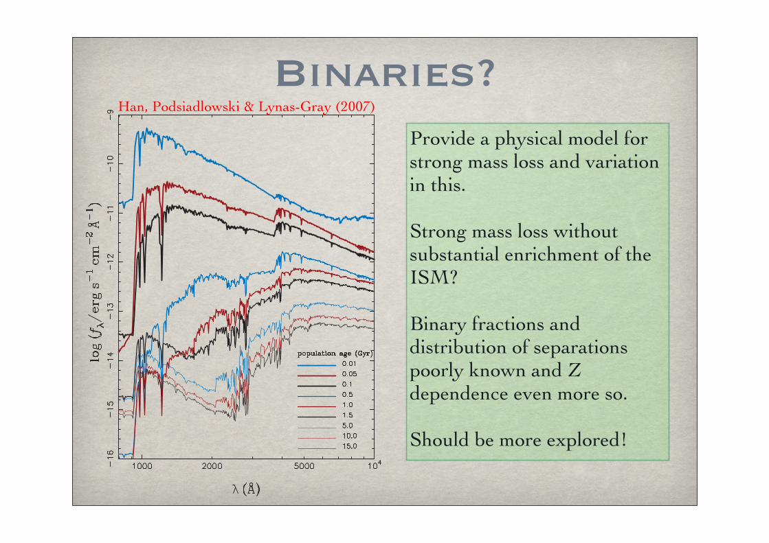
Binaries?Han, Podsiadlowski & Lynas-Gray (2007)
Provide a physical model for strong mass loss and variation in this.
Strong mass loss without substantial enrichment of the ISM?
Binary fractions and distribution of separations poorly known and Z dependence even more so.
Should be more explored!

Binaries?Han, Podsiadlowski & Lynas-Gray (2007)
Provide a physical model for strong mass loss and variation in this.
Strong mass loss without substantial enrichment of the ISM?
Binary fractions and distribution of separations poorly known and Z dependence even more so.
Should be more explored!

The Optical[α/Fe]

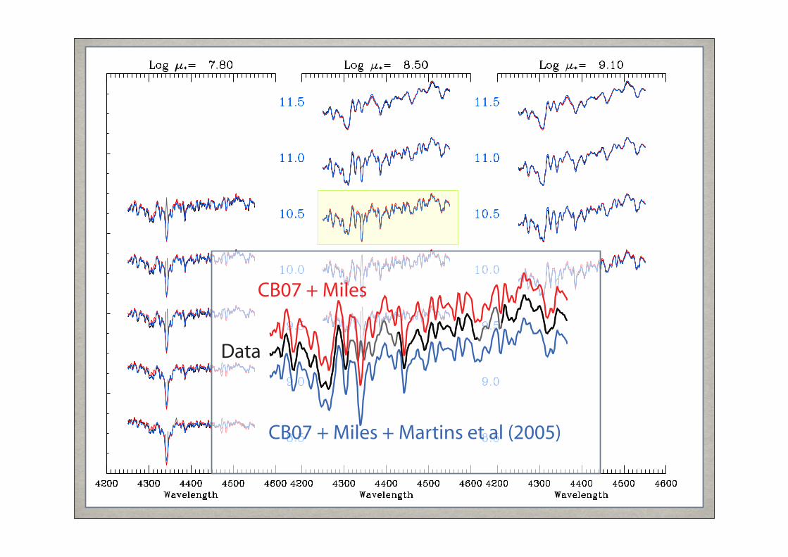
StatusAt first glance in good shape.

StatusAt first glance in good shape.
StatusAt first glance in good shape.
CB07 + Miles
CB07 + Miles + Martins et al (2005)
Data

StatusAt first glance in good shape.
CB07 + Miles
CB07 + Miles + Martins et al (2005)
Data
StatusAt first glance in good shape.

Non-solar α/FeDetermining the age of elliptical galaxies:
Fe-sensitive indices: Lower metallicites & higher agesMg-sensitive indices: Higher metallicites & lower ages
This inconsistency points to variations in Mg/Fe.
Trager et al (2000)
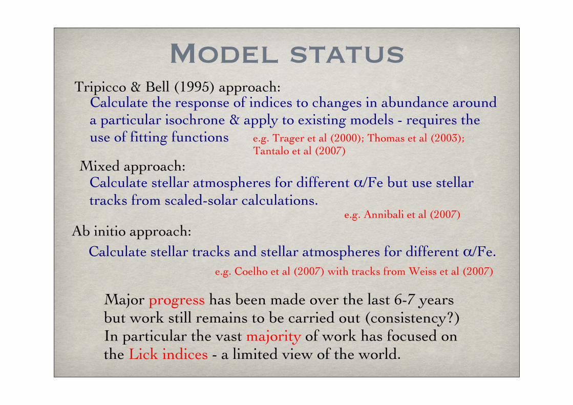
Model statusTripicco & Bell (1995) approach:
Calculate the response of indices to changes in abundance around a particular isochrone & apply to existing models - requires the use of fitting functions e.g. Trager et al (2000); Thomas et al (2003);
Tantalo et al (2007)
Ab initio approach:Calculate stellar tracks and stellar atmospheres for different α/Fe.
Mixed approach:Calculate stellar atmospheres for different α/Fe but use stellar tracks from scaled-solar calculations.
e.g. Annibali et al (2007)
e.g. Coelho et al (2007) with tracks from Weiss et al (2007)
Major progress has been made over the last 6-7 years but work still remains to be carried out (consistency?)In particular the vast majority of work has focused on the Lick indices - a limited view of the world.

Model statusEven models with similar methodology give disparate results:
Trends roughly similar, but absolute values differ significantly...
Possibly due to choice of tracks but this dependence is not fully understood.

Need consistent approach
Coelho et al (2007) - tracks Weiss et al (2007)
[Fe/H] = -0.5
[α/Fe] = 0.4[α/Fe] = 0.0
ΔY/ΔZ?
Enrichment pattern probably not a major issue (but what about advanced phases?)

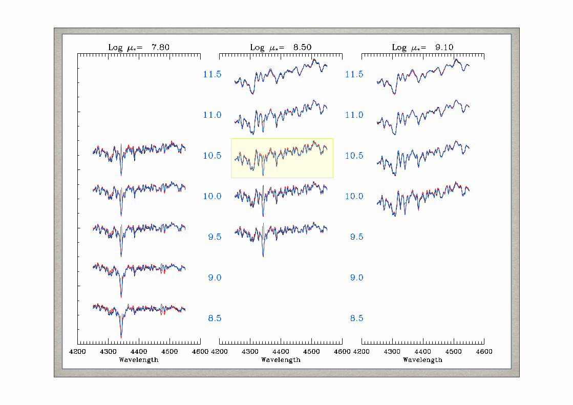
Identify features from data
The data should have better S/N than the models for accurate comparison.
500,000 spectra -> ~1000 Co-adding SDSS:
Result: Typical S/N per Å ~200 [100 - 550Å]
Use Stellar mass & concentration as proxies for non-solar abundance ratios. Most other issues should not correlate with these quantities.
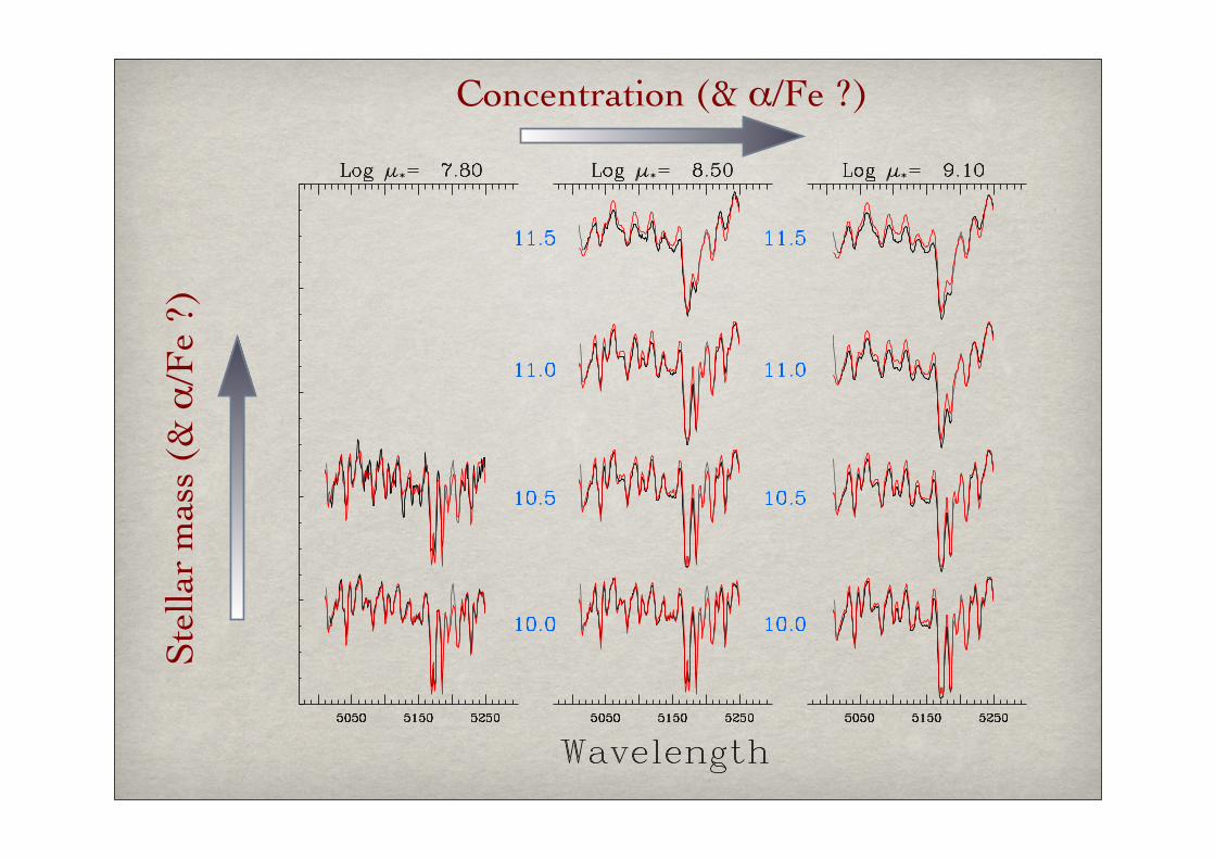
Concentration (& α/Fe ?)
Ste
llar
mas
s (&
α/F
e ?)

Concentration (& α/Fe ?)
Ste
llar
mas
s (&
α/F
e ?)
Mg-indices

Define discrepancy: fobs(λ) - fbest fit(λ)
d(λ) = fobs(λ) This region is
known to be strongly sensitive to Mg/Fe variations.
A similar approach allows identification of features with weak or strong α/Fe dependency.
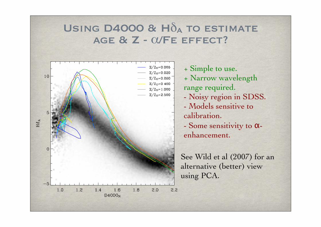
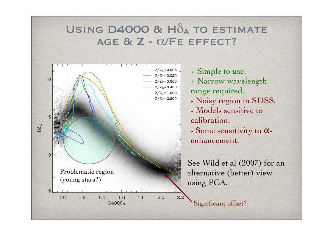
Using D4000 & HδA to estimate age & Z - α/Fe effect?
+ Simple to use.+ Narrow wavelength range required.- Noisy region in SDSS.- Models sensitive to calibration.- Some sensitivity to α-enhancement.
See Wild et al (2007) for an alternative (better) view using PCA.

Using D4000 & HδA to estimate age & Z - α/Fe effect?
+ Simple to use.+ Narrow wavelength range required.- Noisy region in SDSS.- Models sensitive to calibration.- Some sensitivity to α-enhancement.
See Wild et al (2007) for an alternative (better) view using PCA.
Problematic region (young stars?)
Using D4000 & HδA to estimate age & Z - α/Fe effect?
+ Simple to use.+ Narrow wavelength range required.- Noisy region in SDSS.- Models sensitive to calibration.- Some sensitivity to α-enhancement.
Significant offset?
See Wild et al (2007) for an alternative (better) view using PCA.
Problematic region (young stars?)
1 1.5 2 2.5 3 3.5
-10
0
10
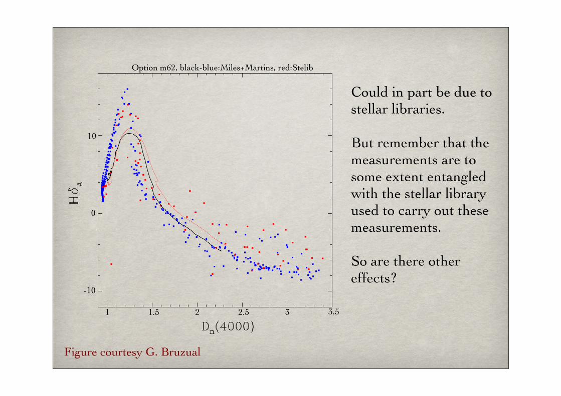
Option m62, black-blue:Miles+Martins, red:Stelib
Could in part be due to stellar libraries.
But remember that the measurements are to some extent entangled with the stellar library used to carry out these measurements.
So are there other effects?
Figure courtesy G. Bruzual
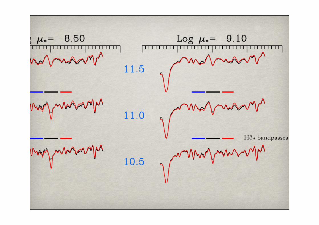
HδA bandpasses

See a discrepancy that increases with mass and with concentration.
This turns out to match very well with the CN band head -> non-solar abundance ratios fit well.
See: L. Prochaska et al (2007) for an in-depth discussion.
HδA bandpasses
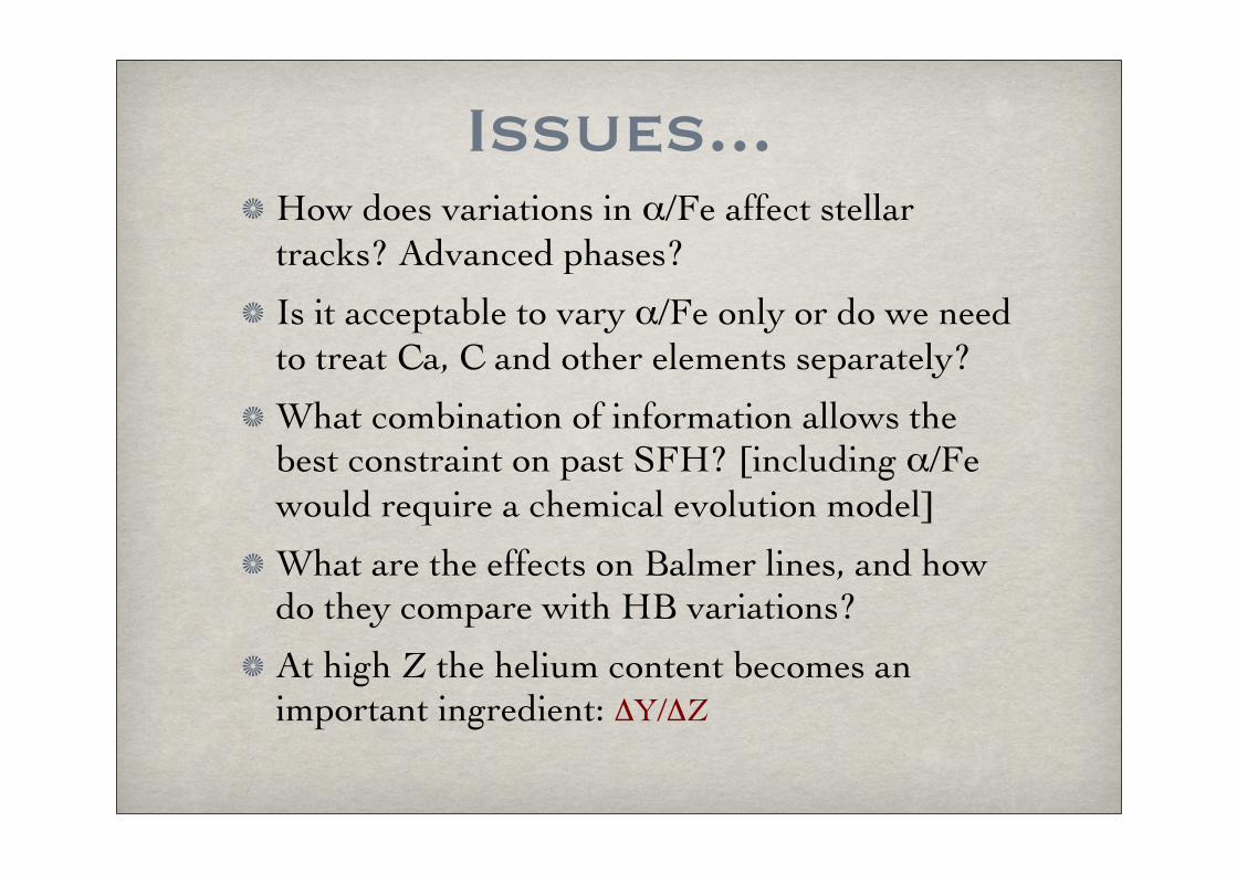
Issues...How does variations in α/Fe affect stellar tracks? Advanced phases?
Is it acceptable to vary α/Fe only or do we need to treat Ca, C and other elements separately?
What combination of information allows the best constraint on past SFH? [including α/Fe would require a chemical evolution model]
What are the effects on Balmer lines, and how do they compare with HB variations?
At high Z the helium content becomes an important ingredient: ΔY/ΔZ

Into the RedThe TP-AGB Phase

TP-AGB Stars
Relatively short-lived & very luminous and cool phase. So gives a characteristic and strong contribution to longer wavelength light.
Herwig (2005, ARA&A)

TP-AGB Stars
TP-AGB
Relatively short-lived & very luminous and cool phase. So gives a characteristic and strong contribution to longer wavelength light.
Herwig (2005, ARA&A)

TP-AGB stars can become very luminous C stars and dominate the MIR light of a stellar population, particularly at low metallicity.
They are very difficult to simulate from first principles so models covering large regions of parameter space use a “synthetic” approach with parameters calibrated by observations - typically C stars.
The properties of the most extreme (TP-)AGB stars and AGB stars at low metallicity are not well known.
Stellar atmospheres for these phases are less well developed and sensitive to dust treatment -> significant uncertainties in the relative contribution of NIR and MIR flux.
The first TP-AGB stars in a population start to appear ~0.5Gyr after the star of star formation and provide >30% of the K-band light for several Gyrs after that.
Age of the Universe at z=2: 3.2 Gyr.
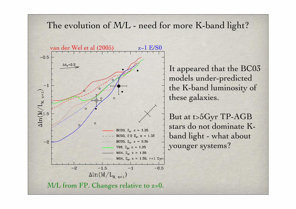
The evolution of M/L - need for more K-band light?
van der Wel et al (2005) z~1 E/S0
It appeared that the BC03 models under-predicted the K-band luminosity of these galaxies.
But at t>5Gyr TP-AGB stars do not dominate K-band light - what about younger systems?
M/L from FP. Changes relative to z=0.

Estimating stellar masses.
As emphasised by Maraston et al (2006), rest-frame NIR photometry of star-forming galaxies is very sensitive to the TP-AGB treatment.
This might cause substantial systematic uncertainties in mass estimates.
Maraston et al (2006, Fig 4 & 5 partial)
If the TP-AGB luminosity is underestimated (as in the old BC03 models), the lack of red flux must be compensated by adding dust and increasing the age.
Adding photometry uncritically is a bad idea - always ask: Will this improve my results?

Improving TP-AGB treatment
Sparse grid of full calculations of TP-AGB stars
Fitting formulae for evolutionary behaviour
Large grids of synthetic models
Predict observational quantities
Compare with observations.
Luminosity function of C-starsLife-times of C-stars (LMC, SMC)+ SFH & Age-Metallicity relation
Dredge-up,Chemical composition, Pulsation modeAge-Z relation
See Marigo & Girardi (2007) for a detailed discussion.

Improving TP-AGB treatment
See Marigo & Girardi (2007) for details.
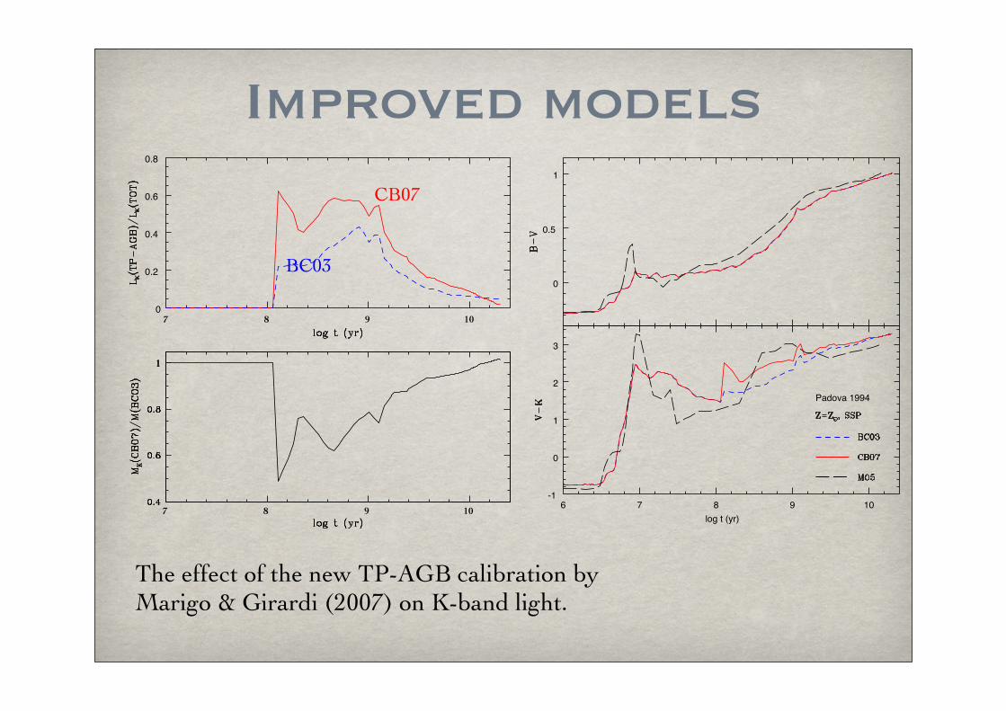
Improved models
7 8 9 10
0
0.2
0.4
0.6
0.8
7 8 9 10
BC03
CB07
0
0.5
1
6 7 8 9 10-1
0
1
2
3
Padova 1994
log t (yr)
The effect of the new TP-AGB calibration by Marigo & Girardi (2007) on K-band light.

But there is more!

Chemical evolutionThe metal content of a galaxy changes with time, and this ought to be taken into account. The problem?
A large number of additional variables, infall, outflow etc. means that there are plenty of degeneracies to deal with - not to speak of spatial variation.
And the detailed chemical output from supernovae and the variability is poorly known (well, unless you ask a modeller!)
Crucial for understanding the MW.
Ought to provide extra constraints on estimates of SFHs.

Chemical evolutionClosed box model with Z=0.02 at t=5Gyr
This becomes important for very high S/N spectra!
0.1
dex

Chemical evolutionClosed box model with Z=0.02 at t=5Gyr
This becomes important for very high S/N spectra!
0.1
dex
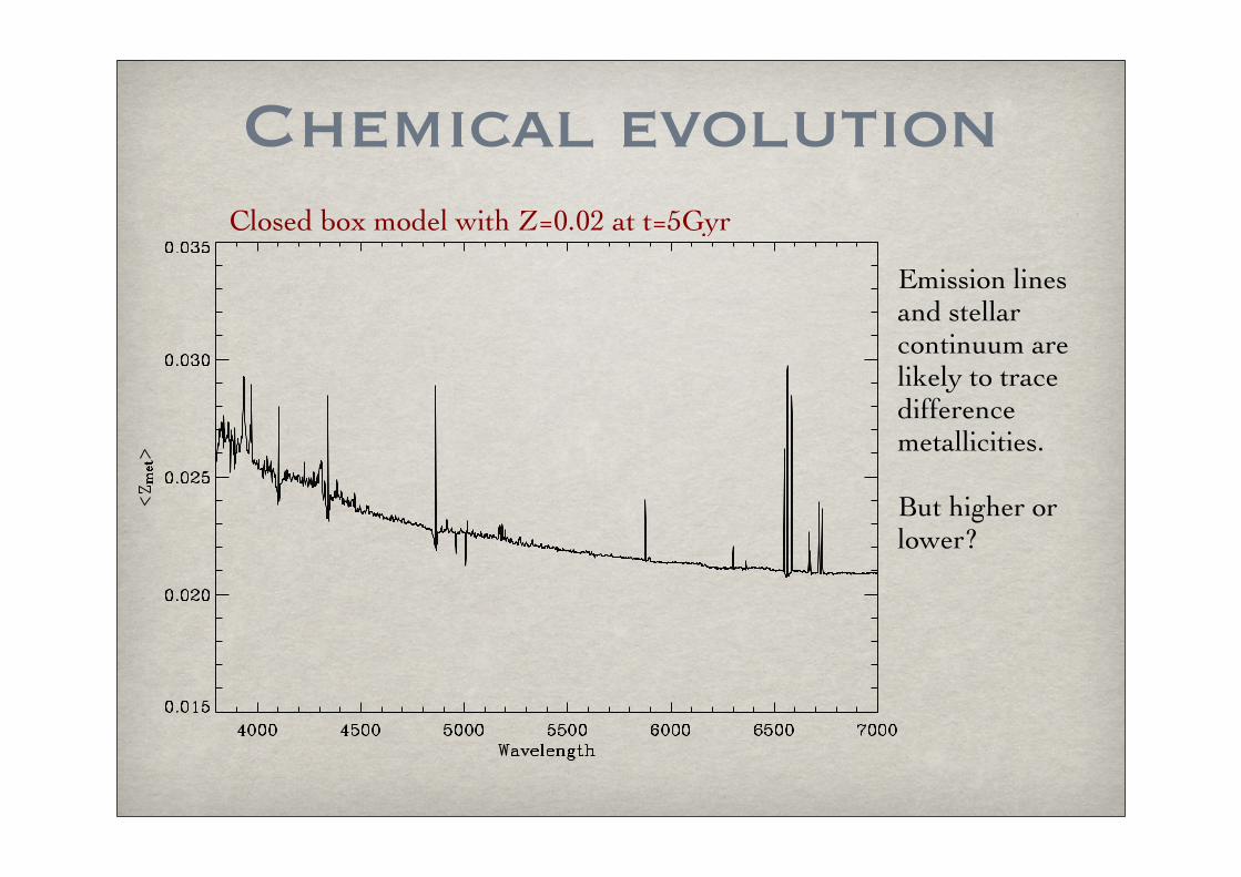
Chemical evolutionClosed box model with Z=0.02 at t=5Gyr
Emission lines and stellar continuum are likely to trace difference metallicities.
But higher or lower?
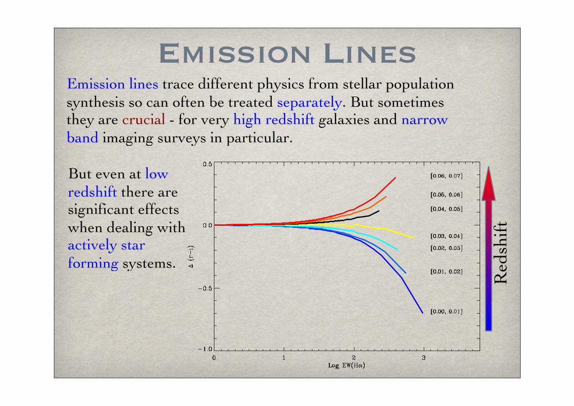
Emission LinesEmission lines trace different physics from stellar population synthesis so can often be treated separately. But sometimes they are crucial - for very high redshift galaxies and narrow band imaging surveys in particular.
But even at low redshift there are significant effects when dealing with actively star forming systems.
Red
shift
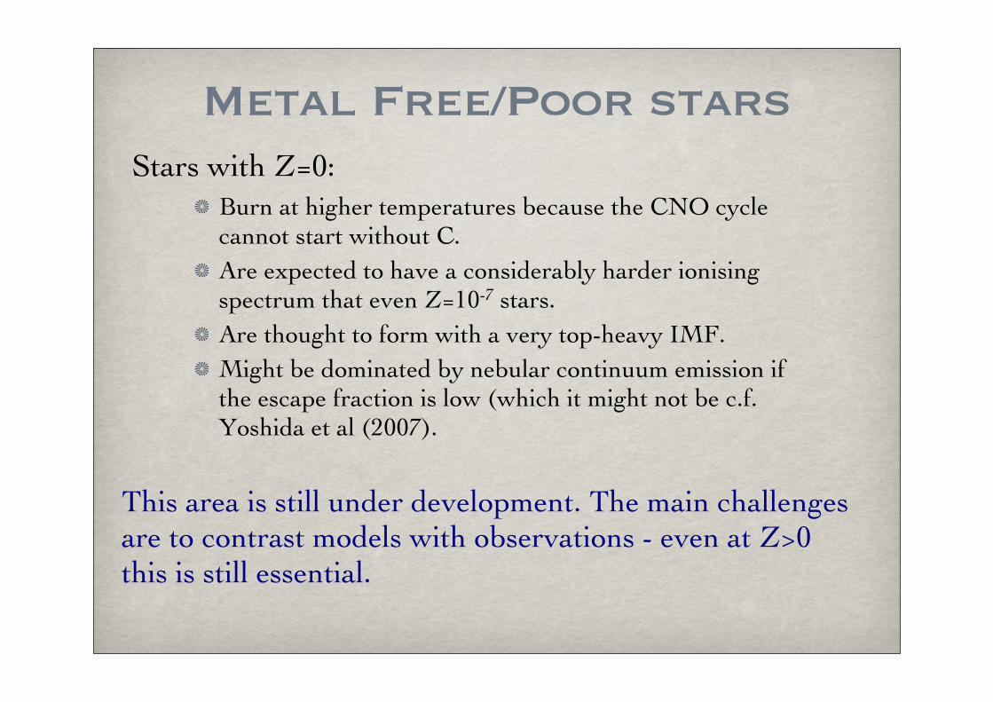
Metal Free/Poor starsStars with Z=0:
Burn at higher temperatures because the CNO cycle cannot start without C.Are expected to have a considerably harder ionising spectrum that even Z=10-7 stars.Are thought to form with a very top-heavy IMF.Might be dominated by nebular continuum emission if the escape fraction is low (which it might not be c.f. Yoshida et al (2007).
This area is still under development. The main challenges are to contrast models with observations - even at Z>0 this is still essential.
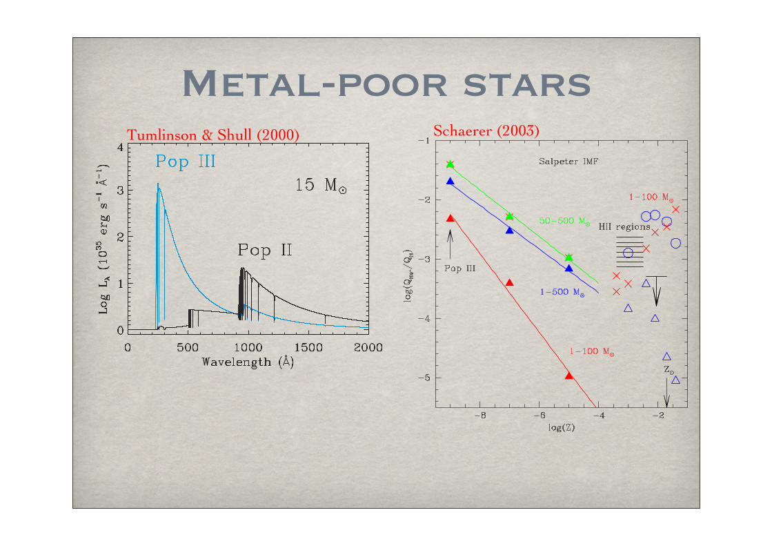
Metal-poor starsTumlinson & Shull (2000) Schaerer (2003)
A Key LessonDo not include an extra wavelength (band) just because you can!
Just because a new instrument becomes available, does not mean that adding information from this will improve your results! You MUST check that the model predictions are reliable for what you need.
But models can be improved so get the data (if you can!) and be critical & constructive!

Status & IssuesStellar rotation & evolutionary tracks?
Binaries & HB morphology?
Resolution - OK? Not yet fully exploited?
TP-AGB - calibrated on LMC/SMC - metallicity variation uncertain - ab initio models not good enough.
α/Fe - progress, but not yet finished.
Reverse use - use observations to constrain poorly known evolutionary phases.
Resolved spectroscopy & separation of different stellar populations in velocity & chemical composition.
Very low-Z populations - empirical tests required.
Uncertainty estimates on predictions?
☝