Models of the Neoclassical synthesis

This lecture presents the standard macroeconomic approach starting with IS-LM model to model of the Phillips curve.→ from IS-LM to AD-AS models without and with dynamics

→ General equilibrium model without explicit micro-foundations of individual decisions and description of market organizations

Plan of the talk

1. Aggregate demand and IS-LM model

2. Oscillator model3. AD-AS model4. Model of the Phillips curve

1. Aggregate Demand and IS-LM Model

● How is aggregate demand determined ?● The IS curve shows the combination of output and

interest rate such that planned and actual expenditures are equal

● The LM curve shows the combination of output and interest rate such that money supply is equal to money demand

The IS curve● Planned expenditures

i= interest rate, T = taxes

→ often written as

● Assume that firms production is used for consumption, investment, government expenditures and inventories for what is left, then actual expenditures are always equal to output→ if planned expenditures are smaller than output, then firms will accumulate unwanted inventories and will therfore cut production→ the equilibrium of the model is obtained for E=Y

The IS curve● The IS curve is downward sloping in the (Y,i) space

● Along the IS curve, we can compute the Keynesian multiplier

● We need another equation to determine Y and i

The LM curve● Money demand = demand for real balances:

● Money supply = exogenous in nominal terms:

● The equation defining LM is(=money market equilibrium)

● By fully differentiating, one gets

The LM curve● For a given price level

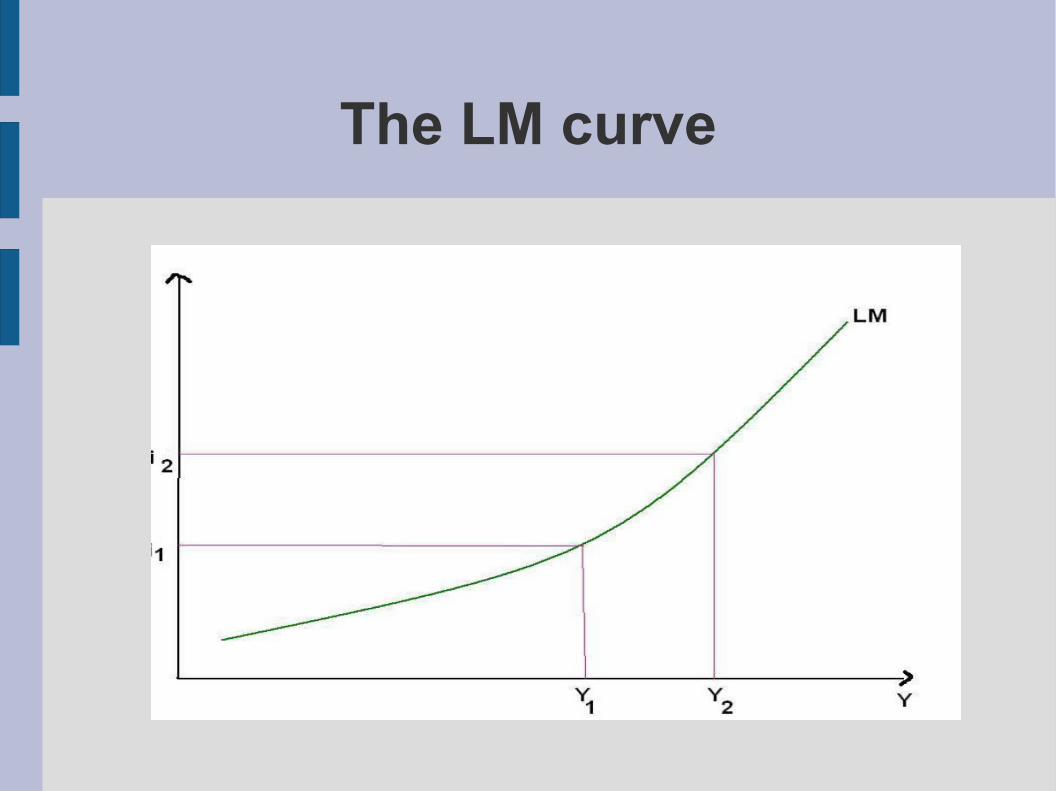
The LM curve

Example: Volcker tight monetary policy

● Paul Volcker was the chairman of the US Fed in the late 70s-early 80s

● 70s: High inflation (11,3% in 1979)● Volcker: tight money policy to fight inflation (announced

in October 1979). Beyond IS-LM, from Quantitative Theory of Money (basic classical economics):

Fischer relation: → « Fischer effect »: a decrease in the money growth of 1% causes a 1% decrease in inflation (QTM), which causes a decrease in the nominal interest rate (Fischer relation)

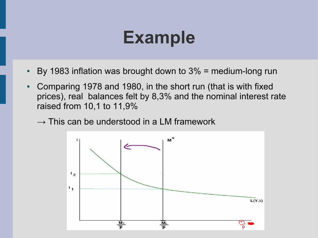
Example● By 1983 inflation was brought down to 3% = medium-long run ● Comparing 1978 and 1980, in the short run (that is with fixed

prices), real balances felt by 8,3% and the nominal interest rate raised from 10,1 to 11,9%

→ This can be understood in a LM framework

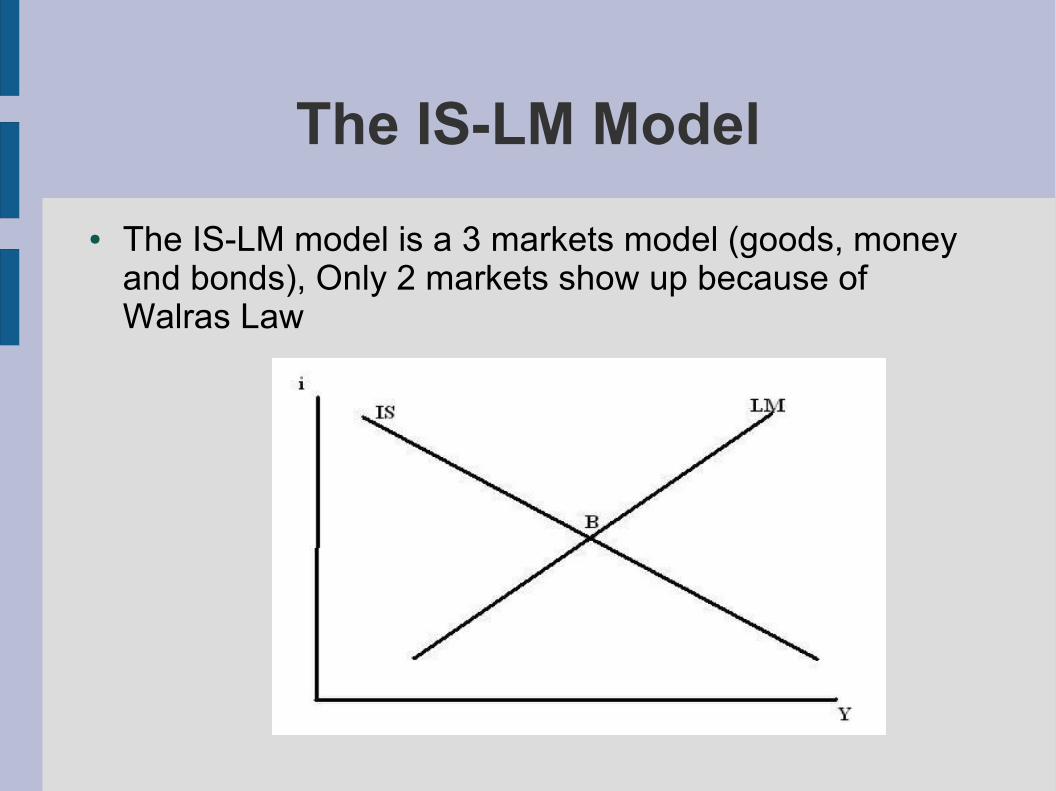
The IS-LM Model● The IS-LM model is a 3 markets model (goods, money

and bonds), Only 2 markets show up because of Walras Law

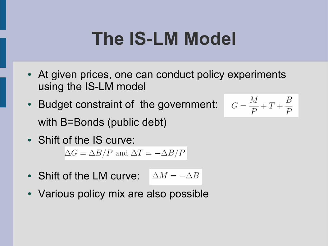
The IS-LM Model● At given prices, one can conduct policy experiments

using the IS-LM model● Budget constraint of the government:

with B=Bonds (public debt)● Shift of the IS curve:

● Shift of the LM curve: ● Various policy mix are also possible

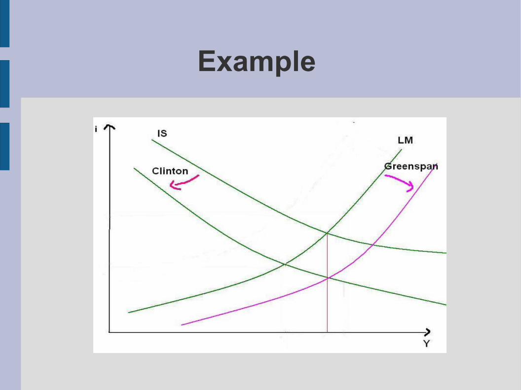
Example: the Clinton-Greenspan policy mix

● Keynesian policy mix is the joint manipulation of IS and LM

● An example is the Clinton-Greenspan policy of 1992-2000

● 1992: the US economy is still thought to be in the 1990-91 recession → historically large federal deficit

Example

● Problem: the need to reduce deficit was likely to deepen the recession

Example● 6 years later, the deficit has disappeared and growth is

large. How can this be understood in a IS-LM setup?

● Greenspan did implicitly commit to ease monetary policy against budgetary restrictions, to undo the recessive impact of budgetary policy→ In 1993, Clinton presented to the Congress a plan of deficit reduction with a -2,5% target in 1998 (both increase in taxes and cuts in expenditures)

Example● The deficit reduction was kept modest because of the

fear of a new recession● The Fed did what was expected: interest rates were

continuously reduced

Example

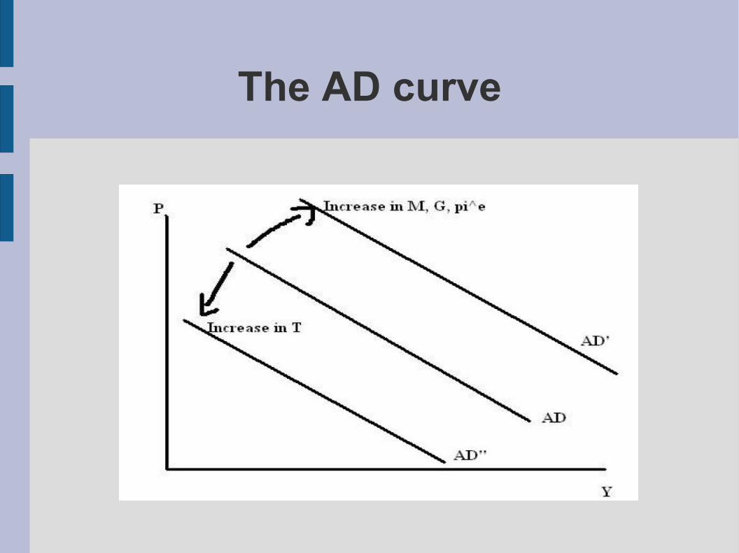
The AD curve● Keynesian models assume that prices are fixed● The AD curve shows the combination of output and

prices such that planned expenditures are equal to output and the money market clears,

● Using IS-LM one can show that the AD curve is downward sloping

The AD curve

2. Oscillator model● The oscillator model is a dynamic version of the IS-LM

model because of an accelerator-type function of investment + lagged consumption function

● ↔ Backward looking expectations (adaptative)

Dynamics of the IS-LM model● The output is solution of the difference equation:

● The solution is the sum of the particular solution

and the solutions to the homogenous equation

● The stationary solution is

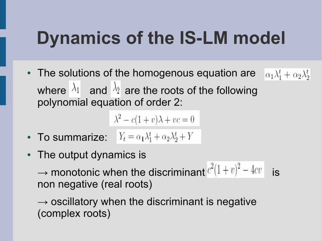
Dynamics of the IS-LM model● The solutions of the homogenous equation are

where and are the roots of the following polynomial equation of order 2:

● To summarize: ● The output dynamics is

→ monotonic when the discriminant is non negative (real roots) → oscillatory when the discriminant is negative (complex roots)

Dynamics of the IS-LM model● converges to Y whathever the intial condition if both

roots are inferior to 1 (=Global stability). If one root is greater than 1 in absolute value (let assume ), there exists a particular condition relying on initial conditions to imply (=local stability)

Monotonic and stable dynamics

Oscillatory and stable dynamics

Oscillatory and unstable dyanmics

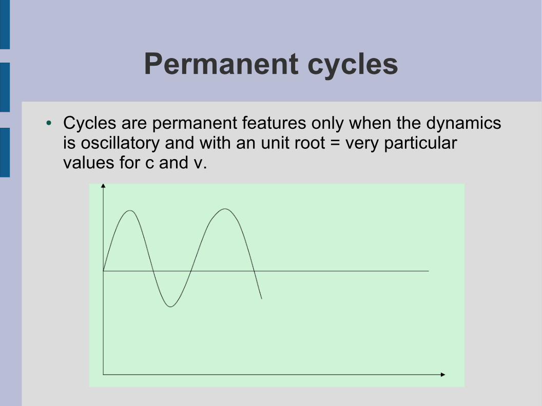
Permanent cycles● Cycles are permanent features only when the dynamics

is oscillatory and with an unit root = very particular values for c and v.

Permanent endogenous cycles

→ no reasons to be verified→ even if the condition holds, the cycles do not look like the observed ones (no constant periodicity and amplitude)

→ Need to go beyond the endogenous cycles hypothesis

Shock-based approach● Moving to stochastic cycles in line of Slutsky and Frisch

experiments inf the 1930s

● These shocks, Frisch and Slutsky argued, are entirely random and distributed normally (standard variation with a mean of 0). This implies that most of shocks are relatively small and approximately half of them were negative and the other half is positive

Shock-based approach● Stochastic non predictable shocks occur regularly and

are propagated across sectors and over time by decisions taken by private agents and governments.

● The oscillator model can be rewritten as follows:

where we take into account of a stochastic component for private investment

● Problems of the approach: models without microfoundations → parameters cannot be considered as invariant to policy changes (Lucas critique)

3.The AD-AS Model● AD= level of aggregate demand as a function of the

general price level

M= money supply, G= government expenditures● AS= level of aggregate supply as a function of the

general price level P

Q= productivity; Y= value added = income = expenditures

● is positive if nominal wages are rigid (see hereafter)

The impact of supply shocks● Impact of a Supply Shock

P

Y

ASAD

OIL SHOCK

TECHNOLOGICAL SHOCK

Macroeconomic policy issues● Impact of a Demand Shock (M,G)

● It raises prices and decreases real wages so that this leads employment and output to increase

● What is central is the value of b1 (which gives the slope of AS)

P

Y

ASAD

The Walrasian case (b1=0)● Assume that labor market clears. For a given P:

● The real wage and the level of employment are determined without any need for the AD curve. The AD curve determines the price level and the composition of aggregate demand.

● The AS curve is veritical, demand policy is ineffective→ it is the Walrasian case

The Walrasian case

The Walrasian case

→ real wages do not respond to demand shocks→ real wages are procyclical following productivity shocks

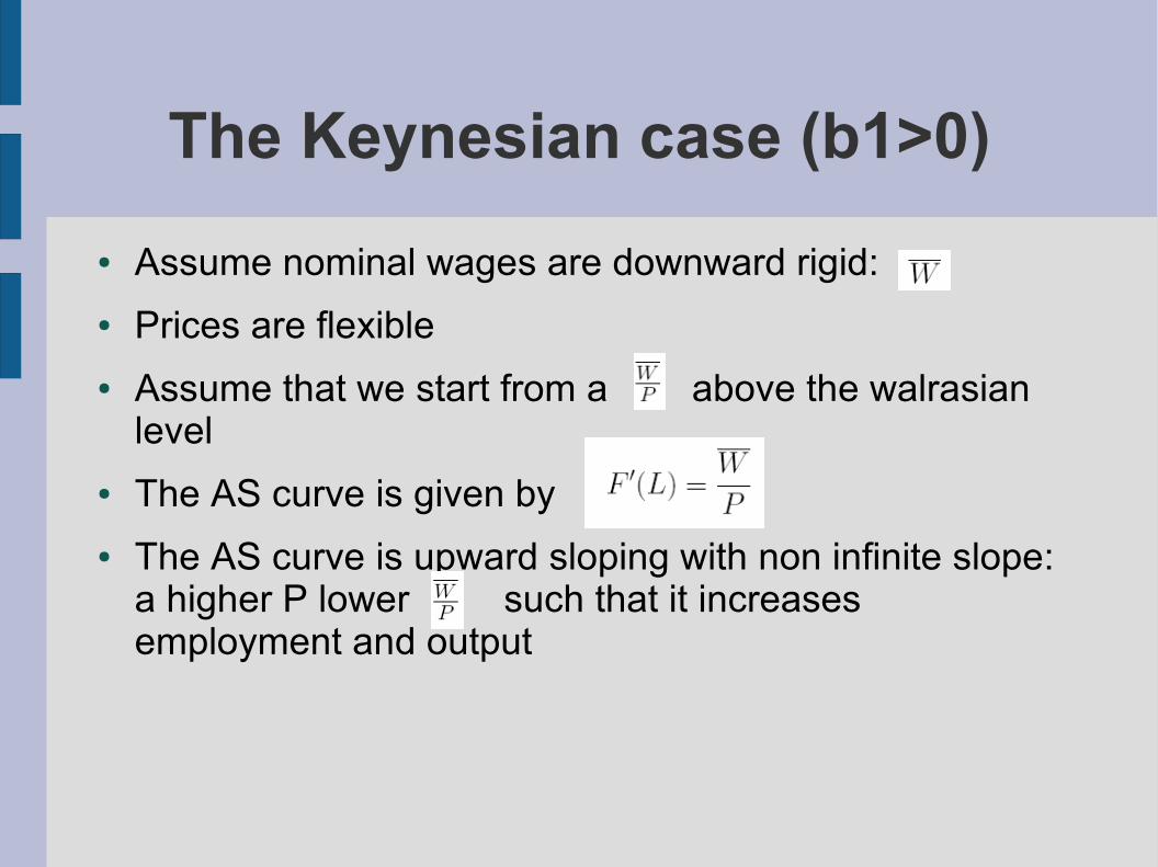
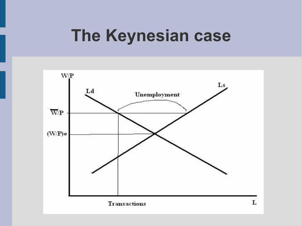
The Keynesian case (b1>0)● Assume nominal wages are downward rigid:● Prices are flexible● Assume that we start from a above the walrasian

level ● The AS curve is given by ● The AS curve is upward sloping with non infinite slope:

a higher P lower such that it increases employment and output

The Keynesian case

The Keynesian case

The Keynesian case● Once P has increased enough for the real wage to

have reached its walrasian level, any subsequent increase in P is followed by an increase in W; the AS curve becomes vertical.

The Keynesian case● The real wage is counter-cyclical following demand

shocks, in contradiction with what is observed on the data.

● One can construct AD-AS models with alternative assumptions on the relative rigidity of prices and nominal wages.

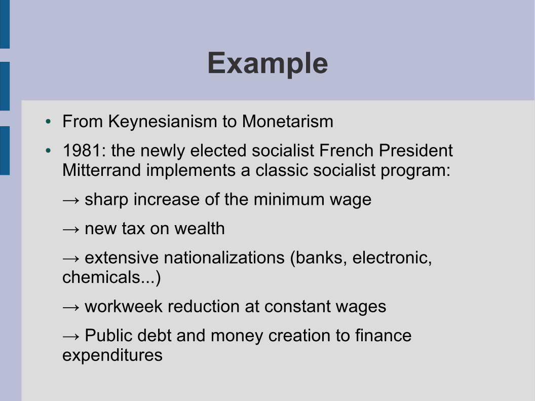
Example● From Keynesianism to Monetarism● 1981: the newly elected socialist French President

Mitterrand implements a classic socialist program:→ sharp increase of the minimum wage→ new tax on wealth

→ extensive nationalizations (banks, electronic, chemicals...)

→ workweek reduction at constant wages→ Public debt and money creation to finance expenditures

Example

Example ● As a consequence, the country experienced higher

inflation than the rest of Europe, but also higher growth

Example ● The problem was then the fixed exchange rate within

the European Monetary System. Even with capital controls, faster money growth leads to larger inflation, and therefore less competitivity given the fixed exchange rate → unemployment

● Deterioration of the current account → 3 devaluations between 1981 and 1983.

● Reversal of policy in 1993: « politique de la rigueur » → freeze government expenditures, increase taxes, wage guidelines to reduce wage pressures, slowdown in money supply growth, reduction of the budget deficit.

4. Model of the Phillips curve● From the observation of Phillips (empirical regularity),

introduce a relation concerning wages adjustement → the AD-AS model augmented by this reduced form equation allows to analysis the short-run and long-run effect of policy shocks.

● The empirical regularity was shown initially by Phillips (1958) on UK data :

The Phillips curve

The Phillips curve

Augmented AS-AD model● Equation of the Phillips curve (Friedman's approach):

where is the expected inflation for t+1● This equation closes the model as providing a

price/wage determination theory and a link between two consecutive static AD-AS equilibria.

● In the long-run, nominal rigidities vanish and the economy is classic, while it is keynesian in the short run.

● Consider a log-linear AD-AS model with a Phillips curve :

● With

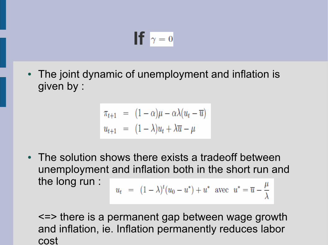
If ● The joint dynamic of unemployment and inflation is

given by :

● The solution shows there exists a tradeoff between unemployment and inflation both in the short run and the long run :

<=> there is a permanent gap between wage growth and inflation, ie. Inflation permanently reduces labor cost

●

●

●

●

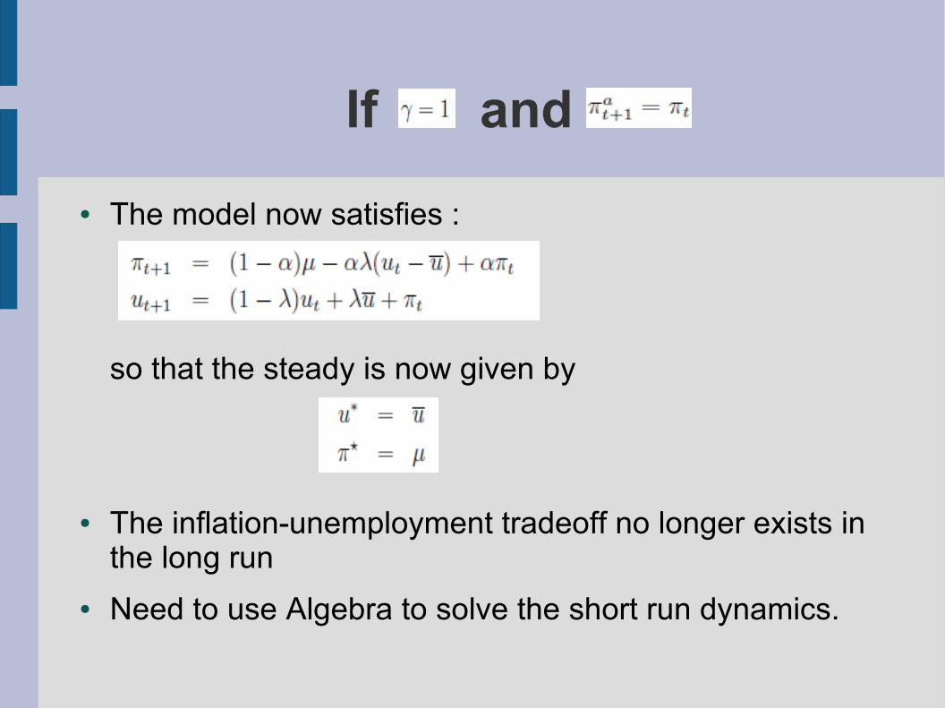
If and

● The model now satisfies :

so that the steady is now given by

● The inflation-unemployment tradeoff no longer exists in the long run

● Need to use Algebra to solve the short run dynamics.

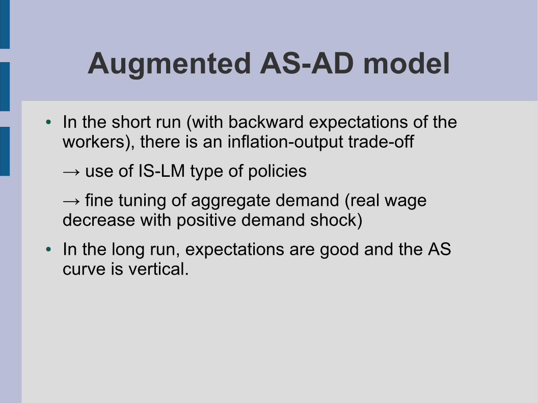
Augmented AS-AD model● In the short run (with backward expectations of the

workers), there is an inflation-output trade-off → use of IS-LM type of policies → fine tuning of aggregate demand (real wage decrease with positive demand shock)

● In the long run, expectations are good and the AS curve is vertical.

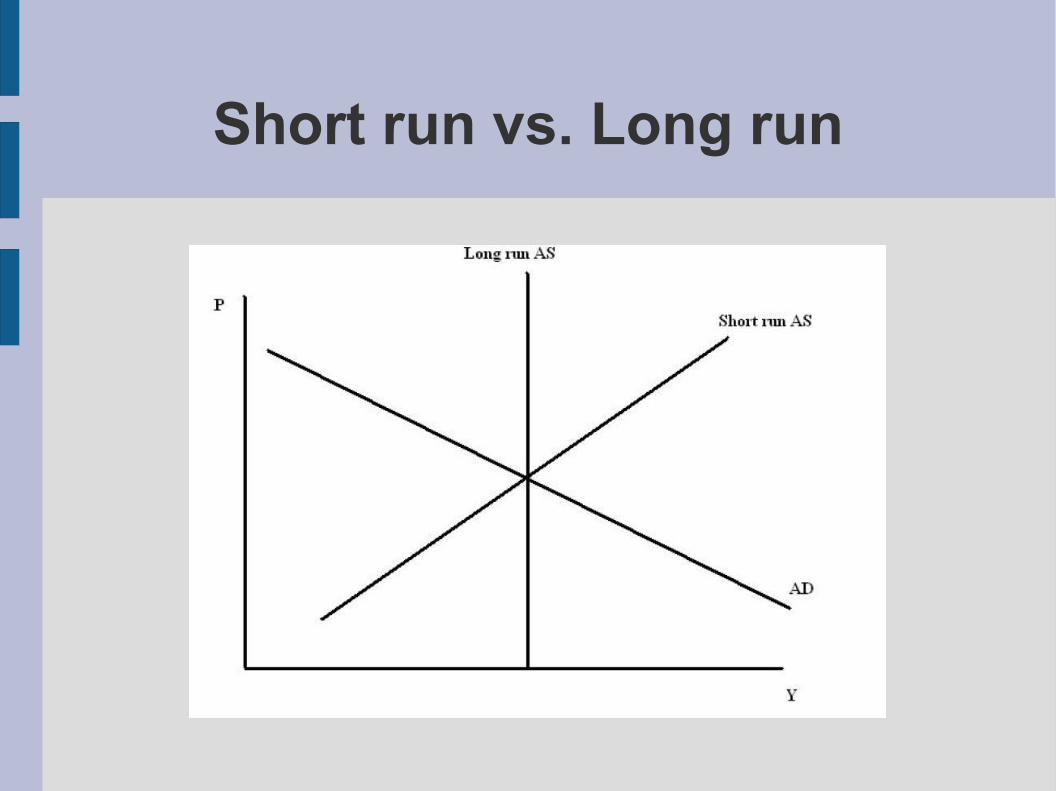
Short run vs. Long run

Conclusion ● This traditionnal view of fluctuations has been seriously

challenged in the late 60s and early 70s.● Different lines of attack: inaccurate description (stagflation =

no growth + inflation), theoretical inconstistencies

→ these attacks come from the New Classical School (Prescott, Lucas, Barro, Sargent...)

→ those first counter models were fully flexible (perfect competition, voluntary unemployment...)

● Most macroeconomists agree now that one can debate over the degree of rigdities or competition, but it is well understood that we undoubtly need to use more micro-dounded models and treat better dynamics and expectations