Embed Size (px)
Citation preview
DISS. ETH NO. 15894
MODELLING OF SPACEBORNE
LINEAR ARRAY SENSORS
A dissertation submitted to the
SWISS FEDERAL INSTITUTE OF TECHNOLOGY ZURICH
for the degree of
Doctor of Technical Sciences
presented by
DANIELA, POLI
Dipl.lng., Politecnico di Milano
born 24.11.1974, citizen of Italy
accepted on the recommendation of
Prof. Dr. Armin Grün, examiner
ETH Zurich, Switzerland
Prof. Dr. Ian Dowman, co-examiner
University College London, United Kingdom
Zurich 2005

Seite Leer /
Blank leaf
CONTENTS
CONTENTS iii
ABSTRACT ix
RIASSUNTO xi
1. INTRODUCTION 1
1.1. REVIEW OF EXISTING MODELS 1
1.2. RESEARCH OBJECTIVES 5
1.3. OUTLINE 7
2. LINEAR CCD ARRAY SENSORS 9
2.1. SOLID-STATE TECHNOLOGY 11
2.2. ARRAY GEOMETRIES 13
2.2.1. Linear arrays 13
2.2.2. Other geometries 18
2.3. IMAGING SYSTEM 21
2.4. SENSOR CALIBRATION 22
2.4.1. Errors in CCD lines 22
2.4.2. Lens distortions 25
2.4.3. Laboratory calibration 26
2.5. STEREO ACQUISITION 28
2.5.1. Across-track 28
2.5.2. Along-track 30
iii

CONTENTS
2.6. PLATFORMS 36
2.6.1. Satellite platforms 37
2.6.2. Airborne and helicopter platforms 41
2.7. IMAGE CHARACTERISTICS 43
2.7.1. Spatial resolution 43
2.7.2. Radiometric resolution 44
2.7.3. Spectral resolution 44
2.7.4. Temporal resolution 46
2.8. PROCESSING LEVELS .-. 47
2.9. LIST OF LINEAR ARRAY SENSORS 47
2.10. CONCLUSIONS 52
3. DIRECT GEOREFERENCING 53
3.1. EXTERNAL ORIENTATION FROM GPS/INS 54
3.1.1. Background 54
3.1.2. GPS system 54
3.1.3. INS system 57
3.1.4. GPS/INS integration 58
3.1.5. Commercial systems 61
3.2. EXTERNAL ORIENTATION FROM EPHEMERIS 62
3.2.1. Orientation with Keplerian elements 63
3.2.2. Orientation from state vectors 65
3.2.3. Interpolation between reference lines 67
3.3. DIRECT GEOREFERENCING 70
3.3.1. From image to camera coordinates 70
3.3.2. From camera to ground coordinates 72
3.3.3. Estimation of approximate ground coordinates 74
3.3.4. Refinement 75
3.4. SOME CONSIDERATIONS ON GPS/INS MEASUREMENTS 76
3.5. ACCURACY EVALUATION 79
3.6. CONCLUSIONS 79
4. INDIRECT GEOREFERENCING 81
4.1. ALGORITHM OVERVIEW 81
4.2. EXTENTION TO MULTI-LENS SENSORS 82
4.3. EXTERNAL ORIENTATION MODELLING 83
4.3.1. Integration of GPS/INS observations 84
4.3.2. Function continuity 86
4.3.3. Reduction of polynomial order 88
4.4. SELF-CALIBRATION 88
iv
CONTENTS
4.5. OBSERVATION EQUATIONS 89
4.5.1. Image coordinates 89
4.5.2. External orientation parameters 89
4.5.3. Self-calibration parameters 91
4.5.4. Ground control points 91
4.6. LEAST SQUARES ADJUSTMENT 92
4.6.1. Theory of least squares adjustment 92
4.6.2. Linearization 94
4.6.3. Design matrix construction 98
4.6.4. Solution of linear system 103
4.7. ANALYSIS OF RESULTS 104
4.7.1. Internal accuracy 104
4.7.2. RMSE calculations 105
4.7.3. Correlations 105
4.7.4. Blunder detection 105
4.8. FORWARD INTERSECTION 106
4.9. SUMMARY AND COMMENTS 107
5. PREPROCESSING 111
5.1. METADATA FILES FORMATS 111
5.2. INFORMATION EXTRACTION FROM METADATA FILES 113
5.3. RADIOMETRIC PREPROCESSING 116
5.3.1. Standard algorithms 116
5.3.2. Ad-hoc filters 117
6. APPLICATIONS 121
6.1. WORKFLOW 122
6.2. MOMS-02 124
6.2.1. Sensor description 124
6.2.2. Data description 126
6.2.3. Preprocessing 127
6.2.4. Image orientation 129
6.2.5. Summary and conclusions 132
6.3. SPOT-5/HRS 133
6.3.1. Sensor description 134
6.3.2. Data description 134
6.3.3. Preprocessing 135
6.3.4. Image orientation 137
6.3.5. DEM generation 139
6.3.6. Comparison 142
6.3.7. Summary and conclusions 146
v

CONTENTS
6.4. ASTER 150
6.4.1. Sensor description 151
6.4.2. Data description 151
6.4.3. Preprocessing 151
6.4.4. Images orientation 153
6.4.5. DEM generation 153
6.4.6. Comparison with reference DEMs 155
6.4.7. Summary and conclusions 159
6.5. MISR 162
6.5.1. Sensor description 162
6.5.2. Data description 163
6.5.3. Preprocessing 164
6.5.4. Image orientation 167
6.5.5. Summary and conclusions 167
6.6. EROS-A1 169
6.6.1. Sensor description 169
6.6.2. Data description and preprocessing 170
6.6.3. Image orientation 172
6.6.4. Summary and conclusions 173
7. CONCLUSIONS AND OUTLOOK 175
7.1. CONCLUSIONS 175
7.2. OUTLOOK 177
Appendix A. ACRONYMS 179
A.1. Sensors and Missions 179
A.2. Space Agencies and Remote Sensing Organizations 180
A.3. Other acronyms 180
Appendix B. REFERENCE SYSTEMS 181
B.1. Image coordinate system 181
B.2. Scanline system 181
B.3. Camera system 182
B.4. Geocentric inertial coordinate system (ECl) 183
B.5. Geocentric fixed coordinate system (ECR) 183
B.6. Geographic coordinates 183
B.7. Local coordinate system 184
B.8. Orbit system 185
B.9. Orbital plane 185
vi

CONTENTS
B.10. GPS coordinate system 185
B.11. INS coordinate system 185
Appendix C. SOFTWARE DESCRIPTION 187
BIBLIOGRAPHY 189
ACKNOWLEDGMENTS 205
vii

CONTENTS
VIII

ABSTRACT
The topic of this research is the development of a mathematical model for the georeferencing of
imagery acquired by multi-line CCD array sensors, carried on air- or spacecraft. Linear array
sensors are digital optical cameras widely used for the acquisition of panchromatic and multi-
spectral images in pushbroom mode with spatial resolution ranging from few centimeters (air¬borne sensors) up to hundreds meters (spaceborne sensors). The images have very high potentialsfor photogrammetric mapping at different scales and for remote sensing applications. For exam¬
ple, they can be used for the generation of Digital Elevation Models (DEM), that represent an
important basis for the creation of Geographic Information Systems, and the production of 3D
texture models for visualization and animation purposes.
In the classical photogrammetric chain that starts from the radiometric preprocessing of the raw
images and goes to the generation of products like the DEMs, the orientation of the images is a
fundamental step and its accuracy is a crucial issue during the evaluation of the entire system.For pushbroom sensors the triangulation and photogrammetric point determination are rather dif¬
ferent compared to the standard approaches for full frame imagery and require special investiga¬tions on the sensor geometry and the acquisition mode.
Today various models based on different approaches have been developed, but few of them are
rigorous and can be used for a wide class of pushbroom sensors. In general a rigorous sensor
model aims to describe the relationship between image and ground coordinates, according to the
physical properties of the image acquisition. The functional model is based on the collinearityequations. The sensor model presented in this thesis had to fulfill the requirement ofbeing rigor¬ous and at the same time as flexible as possible and adaptable to a wide class of linear array sen¬
sors. In fact pushbroom scanners in use show different geometric characteristics (optical systems,number ofCCD lines, scanning mode, stereoscopy) and for each data set specific information are
available (ephemeris, GPS/INS observations, calibration, other internal parameters). Therefore
the model needs to be dependent on a certain number of parameters that may change for each
sensor.
According to the availability of information on the sensor internal and external orientation, the
proposed model includes two different orientation approaches.The first one, the direct georeferencing one, is based on the estimations ofthe ground coordinates
of the points measured in the images through a forward intersection, using the external orienta-
ix

ABSTRACT
tion provided by GPS and INS instruments or interpolated by ephemeris or computed using the
orbital parameters (satellite case). This approach does not require any ground control points,
except for final checking, and does not estimate any additional parameters for the correction of
the interior and exterior orientation. For this reason, the accuracy of this method depends on the
accuracy of the external and internal orientation data.
The alternative orientation method, based on indirect georeferencing, is used if the sensor exter¬
nal and internal orientation is not available or not enough accurate for high-precision photogram¬metric mapping. This approach is a self-calibrating bundle adjustment. The sensor position and
attitude are modelled with 2nd order piecewise polynomial functions (PPM) depending on time.
Constraints on the segment borders assure the continuity of the functions, together with their first
and second derivatives. Using pseudo-observations on the PPM parameters, the polynomialdegree can be reduced to one (linear functions) or even to zero (constant functions). If GPS and
INS are available, they are integrated in the PPM. For the self-calibration, additional parameters
(APs) are used to model the lens internal parameters and distortions and the linear arrays dis¬
placements in the focal plane.The parameters modelling the internal and external orientation, together with the ground coordi¬
nates of tie and control points, are estimated through a least-squares bundle adjustment usingwell distributed ground control points. The use ofpseudo-observations allows the user to run the
adjustment fixing any unknown parameters to certain values. This option is very useful not onlyfor the external orientation modelling, but also for the analysis of the single self-calibration
parameter's influence. The weights for the observations and pseudo-observations are determined
according to the measurement accuracy. A blunder detection procedure is integrated for the auto¬
matic detection ofwrong image coordinate measurement. The adjustment results are analyzed in
terms of internal and external accuracy. The APs to be estimated are chosen according to their
correlations with the other unknown parameters (ground coordinates of tie points and PPM
parameters). A software has been developed under Unix environment in C language.The flexibility of the model has been proved by testing it on MOMS-P2, SPOT-5/HRS, ASTER,MISR and EROS-Al stereo images. These sensors have different characteristics (single-lens andmulti-lens optical systems, various number of linear arrays, synchronous and asynchronousacquisition modes), covering a wide range of possible acquisition geometries.For each dataset both the direct and indirect models have been used and in all cases the direct
georeferencing was not accurate enough for high accurate mapping. The indirect model has been
applied with different ground control points distributions (when possible), varying the PPM con¬
figurations (number of segments, polynomials degree) and with and without self-calibration.
Excluding EROS-Al, all the imagery has been oriented with sub-pixels accuracy in the check
points using a minimum of 6 ground control points. In case of EROS-Al, an accuracy in the
range of 1 to 2 pixels has been achieved, due the lack of information on the geometry of the sen¬
sor asynchronous acquisition. For the ASTER and SPOT-5/HRS datasets, a DEM has also been
generated and compared to some reference DEMs.
New cameras can be easily integrated in the model, because the required sensor information are
accessible in literature as well as in the web. If no information on the sensor internal orientation
is available, the model supposes that the CCD lines are parallel to each other in the focal planeand perpendicular to the flight direction and estimates any systematic error through the self-cali¬
bration. The satellite's position and velocity vectors, usually contained in the ephemeris, are
required in order to compute the initial approximations for the PPM parameters. If this informa¬
tion is not available, the Keplerian elements can be used to estimate the nominal trajectory. For
pushbroom scanners carried on airplane or helicopter the GPS and INS measurements are indis¬
pensable, due to the un-predictability of the trajectory.
x

RIASSUNTO
Il tema di questa ricerca è lo sviluppo di un modello matematico per la georeferenziazione di
immagini acquisite da sensori CCD lineari, montati su aereo o satellite. I sensori lineari sono
strumenti ottici digitali con metodo di acquisizione "pushbroom". Essi sono ampiamente usati
per generare immagini in pancromatico e multispettrale con risoluzione spaziale variabile da
pochi centimetri (sensori su aereo) fino a centinaia di metri (sensori su satellite). Le immaginihanno grandi potenzialita' per la restituzione fotogrammetrica a scale differenti e per varie appli-cazioni nel telerilevamento. Per esempio, esse possono essere usate per la generazione dei mod-
elli digitali delle altezze (DEM), che rappresentano una base importante per la creazione dei
sistemi d'informazione territoriale e la produzione dei modelli 3D per animazioni e di visualizza-
zioni. Nella classica catena fotogrammetrica che inizia con il preprocessamento radiometrico
delle immagini alio stato originale e arriva alla generazione di prodotti come i DEMs, l'orientam-
ento delle immagini è un punto basilare e cruciale per la valutazione di intero sistema. Per i sen¬
sori di tipo pushbroom la triangolazione e il posizionamento fotogrammetrico dei punti sono
piuttosto differenti se confrontati ai metodi standard per i sensori digitali a matrice e richiedono
indagini speciali sulla geometria e sul modo di aquisizione del sensore stesso. Oggi vari modelli
matematici sono disponibili per l'orientamento di sensori pushbroom, ma pochi di loro sono rig-orosi e possono essere usati per una vasta gamma di sensori. In generale, un modello rigorosomira a descrivere il rapporto fra le coordinate immagine e quelle terreno secondo le proprietàfisiche dell'aquisizione dell'immagine. Di conseguenza il modello funzionale è basato sulle
equazioni di collinearita'.
II modello matematico presentato in questa tesi deve soddisfare la condizione di essere rigoroso e
nello stesso momento il piu' possibile flessibile ed adattabile a vari sensori lineari. In effetti glistrumenti a scansione lineare presentano diverse caratteristiche geometriche (sistemi ottici,numéro di linee CCD, metodo di acquisizione, tipo di ricoprimento stereoscopico) con specificheinformazioni ausiliari (effemeridi, osservazioni da GPS/INS, parametri di calibrazione, altri
parametri interni). Di conseguenza il modello deve dipendere da un determinato numéro di
parametri variabili per ogni sensore. A seconda délia disponibilité di informazioni sull'orientam-
ento interno ed esterno dello strumento, il modello proposto include due metodi differenti di geo¬
referenziazione. Il primo, detto diretto, è basato sulla determinazione delle coordinate terreno dei
punti misurati nelle immagini attraverso l'intersezione dei raggi omologhi, usando l'orientamento
XI

RIASSUNTO
esterno fornito dagli strumenti a bordo o interpolato dalle effemeridi o calcolato dai parametriorbitali (caso per satelliti). Questo metodo non richiede punti d'appoggio, eccetto per il controllo
finale, e non estima nessun parametro supplementäre per la correzione deH'orientamento interno
ed esterno. Per questo motivo, l'accuratezza dei risultati dipende dall'accuratezza delle misure di
orientamento interno ed esterno. L'altro metodo di orientamento, basato sulla georeferenziazioneindiretta, è usato se i parametri di orientamento interno ed esterno dello strumento non sono dis-
ponibili o non abbastanza precisi per una restituzione fotogrammetrica di alta precisione. II
metodo indiretto è una compensazione a stelle proiettive con auto-calibrazione. La posizione e
l'assetto dei centri di proiezione sono modellati con segmenti polinomiali di secondo ordine
(PPM) dipendenti dal tempo. Opportuni vincoli sui bordi di ogni segmento assicurano la continu-
ità delle funzioni, insieme alle loro derivate prime e seconde. Usando pseudo-osservazioni sui
parametri PPM, il grado polinomiale puo essere ridotto ad uno (funzioni lineari) o a zero (funzi¬oni costanti). Se le osservazioni da GPS e INS sono disponibili, esse sono integrate nel PPM. Per
l'autocalibrazione, parametri supplementari (APs) modellano le variazioni e le distorsioni delle
lenti ed eventuali spostamenti e rotazioni delle linee CCD nel piano focale. I parametri che
modellano l'orientamento interno ed estemo, insieme alle coordinate terreno dei punti d'appog¬gio e di legame, sono stimati con una compensazione ai minimi quadrati usando punti d'appog¬gio ben distribuai neH'immagine. L'uso di pseudo-osservazioni permette all'operatore di ripeterela compensazione fissando opportuni parametri incogniti a determinati valori. Questa opzione è
molto utile non soltanto per la modellazione deH'orientamento esterno, ma anche per l'analisi
delfinfluenza di ogni singolo parametro aggiuntivo sugli altri. I pesi per le osservazioni e le
pseudo-osservazioni sono determinati dall'accuratezza delle misure. Durante la compensazionegli errori nelle misure delle coordinate immagine sono identificati automaticamente. La compen¬
sazione e' analizzata in termini di accuratezza interna ed esterna. I parametri aggiuntivi da sti-
mare sono scelti a seconda delle loro correlazioni con gli altri parametri incogniti (coordinateoggetto dei punti del legame e dei parametri PPM).Basato su questo modello, un software è stato sviluppato in linguaggio C nel sistema operativoUNIX. La flessibilità del modello è stata dimostrata verificandolo su MOMS-P2, SPOT-5/HRS,
ASTER-VNIR, MISR e EROS-Al. Questi sensori hanno caratteristiche differenti (sistemi ottici
con una o piu' lenti, numéro di linee CCD, acquisizione sincrona ed asincrona) e coprono una
vasta gamma di géométrie di aquisizione. Per ogni dataset sia il metodo diretto che quelloindiretto sono stati usati; in tutti i casi la georeferenziazione diretta non ha dato risultati soddis-
facenti. II metodo indiretto è stato applicato con diverse distribuzioni di punti d'appoggio (sepossibile), variando le configurazioni dei PPM (numéro di segmenti, grado dei polinomi), con e
senza auto-calibrazione. A parte EROS-Al, tutte le immagini sono state orientate con precisioneinferiore al pixel nei punti di controllo usando un numéro minimo di 6 punti d'appoggio. Nel
caso di EROS-Al, l'accuratezza era nell'ordine di 1 - 2 pixel, a causa della mancanza di infor¬
mazioni sulla geometria dell'aquisizione asincrona del sensore. Per SPOT-5/HRS e ASTER, il
corrispondente DEM è stato generato e confrontato con quelli di riferimento e risultati soddis-
facenti sono stati raggiunti. Nuovi sensori lineari possono essere integrati facilmente nel soft¬
ware, poiche' le informazioni necessarie sui sensore sono accessibili in letteratura o in internet.
Se i parametri di calibrazione non sono disponibili, il programma suppone che le linee CCD
siano parallele le une alle altre nel piano focale e perpendicolari alla direzione di volo e stima
l'errore sistematico con un'auto-calibrazione. I vettori di posizione e di velocità del satellite, con¬tenue solitamente nelle effemeridi, sono richiesti per calcolare le approssimazioni iniziali per i
parametri PPM. Se queste informazioni non sono disponibili, gli elementi di Keplero possono
essere usati per valutare la traiettoria nominale. Per i sensori pushbroom montati su aereo o eli-
cottero le misure da GPS e INS sono indispensabili, poiche' la traiettoria non e' completamenteprevedibile.
xii

1
INTRODUCTION
Linear array sensors for Earth observations are widely used for the acquisition of imagery in
pushbroom mode from spaceborne and on airborne platforms. They offer panchromatic and mul-
tispectral images with spatial resolution ranging from few centimeters (airborne sensors) up to
hundreds meters (spaceborne sensors). Images provided by these sensors have very high poten¬tials for photogrammetric mapping at different scales and for remote sensing applications. For
example, they can be used for the generation of Digital Elevation Models (DEM), that representan important basis for the creation of Geographic Information Systems, and the production of3D
texture models for visualization and animation purposes {Grün et al, 2004, Poli et al, 2004b).In the classical photogrammetric chain that starts with the radiometric preprocessing of the raw
images and goes to the generation of products like the DEMs, the orientation of the images is a
fundamental step and its accuracy is a crucial issue during the evaluation of the entire system.For pushbroom sensors the triangulation and photogrammetric point determination are rather dif¬
ferent compared to standard approaches, which are usually applied for full frame imagery, and
require special investigations on the sensor geometry and the acquisition mode.In the next Section the existing approaches followed for the orientation of linear array scanners
are reviewed. Then the main objectives of this research and their development in the thesis are
described.
1.1 REVIEW OF EXISTING MODELS
For the georeferencing of imagery acquired by pushbroom sensors, geometric models with dif¬
ferent complexity, rigor and accuracy have been developed, as described for example in Fritsch
and Stallmann, 2000, Hattori et al, 2000, Dowman and Michaiis, 2003 and Toutin, 2004.
The main approaches are based on rigorous models, Rational Polynomial Models (RPM), Direct
Linear Transformations (DLT) and affine projections.
1

Chapter 1. INTRODUCTION
The rigorous models try to describe the physical properties of the image acquisition. As each
image line is the result of a perspective projection, they are based on the collinearity equations,which are extended in order to include the external (and eventually internal) orientation model¬
ling. Some rigorous models are designed for specific sensors, while some others are more generaland can be used for different sensors. Few models are designed for both spaceborne and airborne
linear scanners.
In case of spaceborne sensors, different approaches have been proposed.In the software SPOTCHECK+, developed by Kratky (Kratky, 1989), the satellite position is
derived from known nominal orbit relations, while the attitude variations are modelled by a sim¬
ple polynomial model (linear or quadratic). For self-calibration two additional parameters are
added: the focal length (camera constant) and the principle point correction. The exterior orienta¬
tion and the additional parameters are determined in a general formulation by least-squaresadjustment. The use of additional information from supplemented data files is not mandatory, but
if this information is available it can be used to approximate or preset some of the unknown
parameters. This model has been used for the orientation of SPOT {Baltsavias and Stallmann,
1992), MOMS-02/D2 (Baltsavias and Stallamann, 1996b), MOMS-02/Priroda (Poli et al,
2000). An advantage of this software is that it can easily integrate new pushbroom instruments, if
the corresponding orbit and sensor parameters are known. The model was also investigated andextended in Fritsch and Stallmann, 2000.
At the Chair of Photogrammetry and Remote Sensing at TU Munich the existing block adjust¬ment program CLIC (TUMunich, 1992) has been extended for the photogrammetric point deter¬
mination of airborne and spaceborne three-line scanners (Ebner et al, 1992). For the external
orientation, a polynomial approach with orbital constraints in case of spaceborne imagery is uti¬
lized. In the airborne case the exterior orientation parameters are estimated only for so-called ori¬
entation points, which are introduced at certain time intervals, e.g. every 100th readout cycle. In
between, the parameters of each 3rd image-line are expressed as polynomial functions (e.g.Lagrange polynomials) of the parameters at the neighboring orientation points. For preprocessedposition and attitude data, like the differential GPS and INS measurements, observation equa¬tions are formulated. Systematic errors of the position and attitude observations are modeled
through additional strip- or block-invariant parameters for each exterior orientation function. 12
parameters are introduced to model a bias and a drift parameter with constant and time-depen¬dent linear terms. For the satellite case, the model exploits the fact that the spacecraft proceedsalong an orbit trajectory and all scanner positions lie on this trajectory, when estimating the
spacecraft's epoch state vector. Due to the lack of a dynamic model describing the camera's atti¬
tude behavior during an imaging sequence, for the spacecraft's attitude the concept oforientation
points is maintained. All unknown parameters are estimated in a bundle block adjustment usingthreefold stereo imagery. The model was tested on MOMS-02/D2 and P2 (Ebner et al, 1992),MEOSS (Ohlhof, 1995), HRSC and WAOSS (Ohlhof and Kornus, 1994) sensors. The same
model has been adopted at DLR for the geometric in-flight calibration and orientation ofMOMS-
2P imagery (Kornus et al, 1999a, Kornus et al, 1999b).The University College London (UCL) suggested a dynamic orbital parameter model (Guganand Dowman, 1988). The satellite movement along the path is described by two orbital parame¬ters (true anomaly and the right ascension of the ascending node) which are modelled with linear
angular changes with time, and included in the collinearity equations. The attitude variations are
described by drift rates. This model was successfully applied for SPOT level 1A and IB,MOMS-02 and IRS-1C (Valadan Zoej and Foomani, 1999) imagery. In (Dowman and Michalis,
2003) this approach was investigated and extended for the development of a general sensor
model for along-track pushbroom sensors. The results obtained with SPOT-5/HRS are reportedin Michail and Dowman, 2004.
2

Section 1.1. REVIEW OF EXISTING MODELS
The IPI Institute in Hannover has developed the program BLASPO for the adjustment of satellite
line scanner images (Konecny et al, 1997). Just the general information about the satellite orbit
together with the view directions in-track and across-track are required. Systematic effects
caused by low frequency motions are handled by self calibration with additional parameters. In
this model the unknown parameters for each image are 14: 6 exterior orientation parameterswhich represent the uniform motion and 8 additional parameters which describe the difference
between the approximate uniform movement and the reality. This program seems very flexible,because it has been used for the orientation of different pushbroom sensors carried on satellite,like MOMS-02 (Büyüksalih and Jacobsen, 2000), SPOT and IRS-1C (Jacobsen et al, 1998),IKONOS and Quickbird (Jacobsen and Passini, 2003), SPOT5-5/HRS (Jacobsen, 2004) and on
airplane, like DPA (Jacobsen and Passini, 2003).Another flexible and rigorous model for pushbroom sensors has been developed by Toutin
(Toutin, 2002) and embedded in PCI Geomatica. The model takes into account the distortions
relative to the platforms (position, velocity, orientation), to the sensor (orientation angles, instan¬
taneous field of view, detection signal integration time), to the Earth (geoid-ellispoid elevation)and the cartographic projection. The unknown parameters are two translations, a rotation related
to the cartographic North, the scale factors and the levelling angles, the non-perpendicularity of
the axes, as well as some 2nd order parameters when the orbital/attitude data are not known or not
accurate (Toutin, 2004).In Westin, 1990 the orbital model used is simpler than in the previous models. A circular orbit
instead of elliptical orbit is used. Using SPOT data, seven unknown parameters need to be com¬
puted for each image.O'Neill (O'Neill andDowman, 1991) proposed a model where auxiliary data are used in order to
set up the relative orientation between the scenes. Then three GCPs are needed to establish the
exterior orientation. The model works accurately with both single SPOT stereo pairs and strips.
Alternative image orientation approaches are based on empirical models (Toutin, 2004). Theydescribe the relation between image and object coordinates and vice versa through• 2D or 3D polynomials or
• the quotients ofpolynomials, usually of 3rd order (Rational Function Model -RFM- or Rational
Polynomial Coefficients - RPC).These empirical models can be used:
• to extract the 2D (or 3D) information from single (or stereo) satellite imagery without explicitreference to either a camera model or satellite ephemeris information and using a large numberofground control points (RFM-1) or
• to approximate the strict sensor model previously developed or contained in the image auxil¬
iary files (RFM-2). A regular grid of the images terrain is first defined and the image coordi¬
nates of the 3D grid ground points are computed using the already-solved 3D physical model,like in SPOTCHECK+ (Kratky, 1989). If the image-to-ground model is available from the
scene auxiliary files (like for SPOT-5/HRG and SPOT-5/HRS), the grid is firstly defined in the
image space and then projected on three different heights in the object space. In both cases, the
image and ground grid points are used as GCPs to resolve the functions and compute the
unknown polynomial terms (Toutin, 2004).In GrodecH and Dial, 2003 a block adjustment with RPC is proposed and applied for the orienta¬
tion of high-resolution satellite stereo images, such as IKONOS. After the determination of the
RPC ofeach image, a block adjustment is applied for the estimation ofa suitable number ofaddi¬
tional parameters. The same model has been implemented at IGP, ETH Zurich, for the orientation
ofIKONOS and Quickbird (Eisenbeiss et al, 2004), SPOT-5/HRS (Poli et al, 2004a) and SPOT-
5/HRG stereo images (Grün et al, 2004).
3

Chapter 1. INTRODUCTION
A special case of 2D/3D empirical models are the affine transformations.
Okamoto (Okamoto, 1981) proposed the affine transformation to overcome problems arising due
to the very narrow field of the sensor view. Under this approach an initial transformation of the
image from a perspective to an affine projection is first performed, then a linear transformation
from image to object space follows, according to the particular affine model adopted. The
assumption is that the satellite travels in a straight path at uniform velocity within the model
space. The model utilizes local systems and ellipsoidal heights as a reference system, therefore
height errors due to the Earth curvature must be compensated. The results demonstrated that 2D
and 3D geopositioning to sub-pixel accuracy can be achieved with IKONOS scenes (Fraser et
al, 2001). The method was applied to SPOT stereo scenes of level 1 and 2 (Okamoto et al,
1998). The theories and procedures of affine-based orientation for satellite line-scanner imageryhave been integrated and used for the orientation MOMS/2P (Hattori et al, 2000) and IKONOS
(Fraser et al, 2001) scenes.
The Direct Linear Transformation (DLT) approach has also been investigated. The solution is
based only on ground control points and does not require the interior orientation parameters nor
the ephemeris information. The DLT approach was suggested for the geometric modelling of
SPOT imagery (El Manadili and Novak, 1996) and applied to IRS-1C images (Savopol and '
Armenakis, 1998). In (Wang, 1999) it was improved by adding corrections for self-calibration.
In general, the approaches based on 2D and 3D empirical models, as those presented, are advan¬
tageous ifthe rigorous sensor model or the parameters of the acquisition system are not available.
Gupta (Gupta and Hartley, 1997) proposed a simple non-iterative model based on the concept of
fundamental matrix for the description of the relative orientation between two stereo scenes. The
model was successfully applied on SPOT scenes. The unknown parameters for each pair are: the
sensor position and attitude ofone scene at the time of acquisition of the first line, the velocity of
the camera, the focal length and the parallax in across-track direction.
In case ofpushbroom sensors carried on airplane or helicopter, GPS and INS (or IMU) observa¬
tions are indispensable, because the airborne trajectories are not predictable. In many cases the
original position and attitude measurements are not enough accurate for high-precision position¬ing and require a correction.
The IGP at ETH Zurich (Grün and Zhang, 2002a) investigated three different approaches for the
external orientation modelling of the Three-Line Scanner (TLS) developed by Starlabo Corpora¬tion: the Direct Georeferencing, in which the translation displacement vector between the GPS
and camera systems is estimated for the correction ofGPS observations, the Lagrange Polynomi¬als, as used in (Ebner et al, 1992) for spaceborne sensors and the Piecewise Polynomials, where
the sensor attitude and position functions are divided in sections and modelled with 1st and 2nd
order polynomials respectively, with constraints on their continuity. The sensor self-calibration
has also been integrated in the processing chain (Kocaman, 2003a). Further investigations on the
models performances are in progress.
In the photogrammetric software for the LH-Systems ADS40 processing, a triangulations is
applied for the compensation of systematic effects in the GPS/IMU observations (Tempelmann et
al, 2000). These effects include the misalignment between IMU and the camera axes and the
datum differences between GPS/IMU and the ground coordinates system. For the orientation of
each sensor line the concept of orientation fixes is used. The external orientation values between
two orientation fixes are determined by interpolation using the IMU/GPS observations.
From the analysis ofthe above literature, which is summarized in Table 1.1, we can see that now¬
adays approaches based on rigorous and non rigorous models are widely used. In case of rigor-
4

Section 1.2. RESEARCH OBJECTIVES
ous models the main research interests are the sensor external and internal orientation modelling.The external orientation parameters are often estimated for suitable so-called "orientation lines"
and interpolated for any other lines. A self-calibration process is often recommended, at least to
model the focal length variation and the first order lens distortions. In order to avoid over-param¬
eterization the correlation between the parameters is investigated and tests on the parameters'significance and determinability are studied. Few models can be applied for both airborne and
spaceborne sensors. The orientation methods based on rational polynomials functions, affine pro¬
jections and DLT transformations are mostly used for high-resolution satellite imagery. They can
be a possible alternative to rigorous models when the calibration data (calibrated focal length,principal point coordinates, lens distortions) are not released by the image providers or when the
sensor positions and attitudes are not available with sufficient precision (Vozikis et al, 2003).
1.2 RESEARCH OBJECTIVES
The topic of this research is the development of a mathematical model for the georeferencing of
imagery acquired by multi-line CCD array sensors, carried on air- or spacecraft. The model has
to fulfill the requirement of being as flexible as possible and being adaptable to a wide class of
linear array sensors. In fact pushbroom scanners in use show different geometric characteristics
(optical systems, number of CCD lines, scanning mode, stereoscopy) and for each data set spe¬
cific information are available (ephemeris, GPS/INS observations, calibration, other internal
parameters). Therefore the model needs to be dependent on a certain number of parameters that
may change for each sensor.
For the orientation of CCD linear array sensors' imagery with a rigorous photogrammetricmodel, the collinearity equations, which describe the perspective acquisition of each image line,will be the basis of the functional model. According to the availability of information on the sen¬
sor internal and external orientation, two approaches must be investigated.The first one, the direct georeferencing one, is based on the estimation of the ground coordinates
of the points measured in the images through a forward intersection, using the external orienta¬
tion provided by GPS and INS instruments or interpolated by ephemeris or computed using the
orbital parameters (satellite case). The advantage of this method is that no ground information is
required, but the results accuracy depends on the precision and availability of the external and
internal orientation information.
On the other hand, in the indirect georeferencing approach, the parameters modelling the internal
and external orientation are estimated in a bundle adjustment with least squares methods. The
external orientation modelling takes into account the physical properties of satellite orbits and the
integration ofobservations on the external orientation, provided by instruments carried on board,while the internal orientation modelling considers the lens distortions and the CCD lines (or seg¬
ments) displacement in the focal plane (or planes).As a result, a flexible model for the orientation of a wide class of pushbroom sensors will be
developed.
5

Tabic
1.1.Summaryofthemaincharacteristics(basic
geometry,externalandinternal
orientationmo
dell
ing,
flexibility)
offourapproaches
fortheorientationof
pushbroomim
ager
y:ri
goro
usmo
dels
,RFM,DLTandaffinemodels.Examples
arealsogi
ven.
Rigorous
RFM
DLT
Affine
RFM-1
RFM-2
Basicgeometry
Perspectivepr
ojection
ineach
line,parallel
projection
between
lines
None
Cameramodel
inauxiliary
files
Proj
ecti
vegeometry
Affinepr
ojec
tion
Mathematical
model
Coll
inea
rity
equationsextended
toincludeinternalandexternal
orientationmodeling
Leastsquaressolution
GCPs
requ
ired
Relationship
betweenimage
(line.sampie)andground
coordinatesthroughquotientsofpolynomials(max
3rd
order)
Rela
tion
ship
between
image(l
ine.
samp
ie)and
groundcoordinates
thro
ughqu
otie
ntsof
1st
orderpo
lyno
mial
s
Rela
tion
ship
between
imageandgroundcoor¬
dinatesthrough2D-3D
affinetransformations
Need
ofGCP
yes,variablenumber
yes,largenumber
only
forrefineme
nt,min2
yes,min6
yes,min3
External
orientation
Modelledwithpiecewisepoly¬
nomi
als,
Lagrangepo
lyno
mial
sorwithconstantsh
ifts
/mis
alig
n¬ments
Same/differentapproach
for
posi
tion
and
attitude
Metadata
filesrequired
(sat
el¬
lite)
PossibleGPS/INS
integration
Notmodelled
NoGPS/INS
integration
Constantshiftsandmis¬
alignmentscompensated
withblockad
just
ment
Nomodel
Constant
shifts
andmis¬
alig
nmen
tscompensated
NoGPS/INS
inte
grat
ion
Traj
ecto
rywithstraight
pathanduniformveloc¬
ityisassumed
Additionalparameters
maybeintroduced
NoGPS/INS
inte
grat
ion
Internal
orientation
Notal
ways
.Mainparameters:
focalle
ngth
,prin
cipa
lpointdi
s¬
placement,
line
curvature
Effectscompensated
in
upper-orderterms
Residual
internalorienta¬
tioncompensated
inblock
adjustment
Notmodelled
Notmodelled
Additionalparameters
forself-calibration
Flex
ibil
ity
Modelsareusuallyse
para
tely
implemented
forspaceborne
andairborneplatforms
Fewmodels
forbothplatforms
High
flexibility
Usua
llyforhigh-resolution
satelliteimagery
High
flex
ibil
ity,because
cameramodeland
satel¬
liteephemerisarenot
requ
ired
High
flex
ibil
ity,because
cameramodel
isnot
requ
ired
Examples
Spotcheck+
CLIC(TU-Munich)
BLUH/BLASPO
(IPI
Hann
over
),UCL,
Toutin'smodel
inPCIGeomat-
ics
ETH-IGPmodels
Specific
modelsfromspace
agencies
Variousexamples
inlitera¬
ture
Krat
ky,1989
GrodeckiandDi
al,2003
ETH-IGP
Someexamples
inlitera¬
ture
ETH-IGP
Wang,1999
ElManadiliandNovak,
1996
Savo
polandArmenakis,
1998
Variousexamples
inlit¬
erature
ETH-IGP
Univ
ersi
tyofMelbourne
Okamoto,1981

Section 1.3. OUTLINE
1.3 OUTLINE
This thesis describes the rigorous sensor model developed at IGP for the orientation of imageryacquired by linear array sensors. A software has been designed, self-implemented in C languageand tested on simulated and real data. The work is described in six chapters.Following this Introduction, in Chapter 2 the main characteristics of linear array sensors are
investigated. This study is required in order to understand the geometric properties of imageryprovided by linear scanners and the range ofcase studies that may occur.
In Chapter 3 the direct georeferencing approach for the orientation ofpushbroom images without
ground control points is described. The alternative approach, the indirect georeferencing model,is proposed in Chapter 4. The functional and stochastic models are both analyzed.After the overview of the preprocessing required for the preparation of the input data (Chapter 5),in Chapter 6 the results of the orientation ofpushbroom imagery from five different satellite sen¬
sors (MOMS-P2, SPOT-5/HRS, ASTER, MISR, EROS-Al) are reported. In order to demon¬
strate the general character and the flexibility of the model, the imagery used come from sensors
with different characteristics (multi-line and single-line sensors at different ground resolution
with synchronous and asynchronous acquisition modes). The internal and external accuracy
obtained for each dataset are reported and commented. The results obtained with airborne pushb¬room imagery are described in Poli, 2002b.
Chapter 6 will close the thesis with some conclusions and future work.
In the Appendices, after the acronyms adopted in the thesis (Appendix A), the main reference
systems mentioned in the thesis are reported (Appendix B) and the software is briefly described
(Appendix C).
7

Chapter!. INTRODUCTION
8

2
LINEAR CCD ARRAY SENSORS
Linear array sensors are widely used for the acquisition of images at different ground resolution
for photogrammetric mapping and remote sensing applications. Today a large variety of sensors
observe the Earth and provide data-for studies of the atmosphere, oceans and land. To classifythese sensors (Figure 2.1), a first distinction can be made between active and passive acquisitionmodes. In passive sensors the energy leading to the received radiation comes from an external
source, e.g. the Sun; on the contrary in active sensors the energy is generated within the sensor
system, beamed outward, and the fraction returned is measured. Both active and passive sensors
can be imaging or non-imaging, according to the production ofimages or not. A sensor classified
as a combination of passive, non-scanning and non-imaging method is a type of profile recorder,for example a microwave radiometer. A sensor classified as passive and imaging is a camera,
such as a close-range or an aerial survey or a space camera. An example of an active and non¬
imaging sensor is a profile recorder such as a laser spectrometer and laser altimeter, while a
radar, for example synthetic aperture radar (SAR), is classified as active and imaging.Going further in the classification of passive imaging sensors, they can be optical and non-opti¬cal, according to the presence ofan optical system or not. In the class ofoptical sensors, the alter¬
native is between film-based and digital cameras. Linear array sensors belong to the category of
the digital optical cameras and acquire in pushbroom mode. The technology used for the digital
acquisition is described in Section 2.1.
In the category of digital optical sensors we also find the point-based electromechanical and the
frame sensors (Section 2.2.2). In the case of a point-based electromechanical scanning system,the image is formed by a side-to-side scanning movement as the platform travels along its path.As frame cameras concern, the images are acquired in digital form with a central perspective,like in case of film-based cameras.
9

Chapter 2. LINEAR CCD ARRAY SENSORS
r Passive
Sensort/pe -
Non-imaging
Microwave radiometer
Magnetic sensor
Gravimeter
Fourier spectrometer
Others
LImaging
r Optical
L Non-optical
L- D
Film-based
igital
— Point-based
— Linear array
— Frame
Microwave radiometer
L Active
r Non-Imaging -
Imaging
r Microwave altimeter
Microwave radiometer
Laser water depth meter
L- Laser distance meter
P Optical Hybrid systems (I.e. Iaser+ frame sei
Phased array radar
L Non-optical —]— Read aperture radar
Synthetic aperture radar
Figure 2.1. Classification of sensors for data acquisition.
-E
In this Chapter the main characteristics of linear array sensors, or linear scanners, and their imag¬
ery are investigated, giving more attention to those aspects that must be taken into account duringthe geometric modelling of this kind of imagery. As the instruments concern, we will concentrate
on the imaging components: the optical system and the linear arrays. The geometry of the solid-
state lines and the optical systems are illustrated in Section 2.2 and Section 2.3. The geometricerrors occurring both in the solid-state lines and in the optical systems are analyzed in Section
2.4, together with two examples of laboratory geometric calibration.
Linear array sensors produce strips with two possible stereo geometries: along and across the
flight direction. These two modes are described in Section 2.5.
Linear array sensors are usually mounted on platforms in the air and in space. Aerial platformsare primarily stable wing aircraft, although helicopters are also used. The aircraft are often used
to collect very detailed images and facilitate the collection of data over virtually any portion of
the Earth's surface at any time. In space, the acquisition of images is sometimes conducted from
the space shuttle or, more commonly, from satellites for Earth observation. Because of their
orbits, satellites permit repetitive coverage ofthe Earth's surface on a continuing basis. This topicwill be addressed in Section
.
The geometric characteristics of the pushbroom sensors and their platforms determine the prop¬
erties ofthe imagery described in Section 2.7. The images are available on the market at different
processing levels (Section 2.8). In conclusion, the principal characteristics ofthe linear array sen¬
sors used in photogrammetry and remote sensing are summarized in Section 2.9.
10

Section 2.1. SOLID-STATE TECHNOLOGY
2.1 SOLID-STATE TECHNOLOGY
George Smith and Willard Boyle invented the Charge-Coupled Device (CCD) at Bell Labs in
1969. They were attempting to create a new kind ofsemiconductor memory for computers and at
the same time to develop solid-state cameras for use in video telephone service. They sketched
out the CCD's basic structure, defined its principles of operation and outlined applicationsincluding imaging as well as memory. By 1970, the Bell Labs researchers had built the CCD into
the world's first solid-state video camera. In 1975, they demonstrated the first CCD camera with
image quality sharp enough for broadcast television. Today, CCD technology is pervasive not
only in broadcasting but also in video applications that range from security monitoring to high-definition television, and from endoscopy to desktop videoconferencing. Facsimile machines,
copying machines, image scanners, digital still cameras, and bar code readers also have
employed CCDs to turn patterns of light into useful information. In general CCD technologiesand image sensors have evolved towards mature products which today can be found in almost all
electronic image acquisition systems (Blanc, 2001). In particular, the combination of CCD and
optical technologies brought the generation of digital optical cameras. Since 1983, when tele¬
scopes were first outfitted with solid-state cameras, CCDs have enabled astronomers to study
objects thousands of times fainter than what the most sensitive photographic plates could cap¬
ture, and to image in seconds what would have taken hours before. Today all optical observato¬
ries, including the Hubble Space Telescope, rely on digital information systems built around
"mosaics" of ultrasensitive CCD chips. CCD cameras are also used in satellite observation of the
earth for environmental monitoring, surveying, and surveillance.
The Charge-Coupled Device is an electronic device made of silicon, capable of transforming a
light pattern into an electric charge pattern (an electronic image). The CCD consists of several
individual photosensitive elements that have the capability of collecting, storing and transportingelectrical charge from one element to another. When the incoming radiation interacts with a CCD
during a short time interval (exposure time), the electronic charges develop with a magnitude
proportional to the intensity of the radiation. Then the charge is transferred to a readout registerand amplified for the analog-to-digital converter (Figure 2.2a). Each photosensitive element will
then represent a picture element (pixel). The chips contain from 3000 to more than 10000 detec¬
tor elements that can occupy linear space less than 15cm in length. With semiconductor technol¬
ogies and design rules, structures that form lines or matrices ofpixels are made.
In photogrammetry and remote sensing the CCD technology is employed almost everywhere. In
close-range the CCD cameras are used for motion capture, human body modelling and objectmodelling for medical, industrial, archeological and architecture applications. On airborne, heli¬
copter and satellite platforms the CCD sensors acquire imagery for terrain models generation and
object extraction.
More recently, alternative sensors based on CMOS (Complementary Metal-Oxide Semiconduc¬
tor) technology have gained considerable interest. CMOS detectors operate at a lower voltagethan CCDs, reducing power consumption for portable applications. Each CMOS active pixel sen¬
sor cell has its own buffer amplifier and can be addressed and read individually (Figure 2.2b).CMOS technology is advantageous for the acquisition of color and false color images. In fact one
of the main difference between CCD and CMOS technology is the generation of color images.Using CCD chips different techniques can be used to obtain color images. One of the most popu¬
lar is the use of an interpolation procedure in conjunction with a mosaic of tiny (pixel-sized)color filters placed over the array of detectors. However this affects the quality of the resulting
image. Another commonly employed solution is to use multiple digital cameras, with each cam¬
era recording a specific spectral band to make up the final composite color or false-color imagewhich is produced by image processing. Needless to say, having to use multiple cameras and fil-
11

Chapter 2. LINEAR CCD ARRAY SENSORS
ters is costly and may be inconvenient. Usually it results in the format size being reduced with
consequent reduction in the ground resolution or ground coverage of the resulting aerial images.On the other hand the three-layer CMOS areal array corresponds to the three-layer color or false-
color photographic emulsion.
amplifier
%>V
v
V V
amplifiers
Figure 2.2. CCD (right) and CMOS (left) detectors. Example with frame chips.
Regarding the development of CCD and CMOS technologies, CCDs have been the dominant
solid-state imagers since the 1970s, primarily because CCDs gave far superior images with the
fabrication technology available. CMOS image sensors required more uniformity and smaller
features than silicon wafer foundries could deliver at the time. Only recently the semiconductor
fabrication has advanced to the point that CMOS image sensors can be useful and cost-effective
in some mid-performance imaging applications. Today the CMOS technology is mostly used in
frame design for close-range applications and lately in some airborne frame cameras too. Cur¬
rently CMOS are not used for space cameras.
In general, as suggested by Litwiller, 2002, CCDs offer superior image performance (as mea¬
sured in quantum efficiency and noise) and flexibility at the expense ofsystem size. They remain
the most suitable technology for high-end imaging applications, such as digital photography,broadcast television, high-performance industrial imaging and most scientific and medical appli¬cations.
CMOS imagers offer more integration (more functions on the chip), lower power dissipation (atthe chip level) and smaller system size at the expense of image quality and flexibility. They are
the technology of choice for high-volume, space constrained applications where image quality
requirements are low. This makes them a natural fit for security cameras, PC videoconferencing,wireless handheld device videoconferencing, bar-code scanners, fax machines, consumer scan¬
ners, toys, biometrics and some automotive in-vehicle uses. Costs are similar at the chip level.
The early CMOS proponents claimed that CMOS imagers would be much cheaper because theycould be produced on the same high-volume wafer processing lines as mainstream logic or mem¬
ory chips. Anyway, the accommodations required for good imaging performance have limited
CMOS imagers to specialized, lower-volume mixed-signal fabrication processes. CMOS imag¬ers also require more silicon per pixel and even if they may require fewer components and less
power, they may also require post-processing circuits to compensate for the lower image quality.The larger issue around pricing is sustainability. The money and attention concentrated on
CMOS imagers mean that their performance will continue to improve, eventually blurring the
line between CCD and CMOS image quality. But for the foreseeable future, CCDs and CMOS
will remain complementary. Each can provide benefits that the other cannot.
In this thesis, only sensor based on CCD technology are taken into account, because currently
(September 2004) CMOS technology is not used in linear array sensors carried on airborne and
satellite for Earth observation. CMOS sensors in linear arrays are used for close range applica¬tions only.
12

Section 2.2. ARRAY GEOMETRES
2.2 ARRAY GEOMETRIES
For the purposes of this thesis, CCDs in the form of linear arrays are investigated (Section 2.2.1).The other CCD designs will be briefly described in Section 2.2.2.
2.2.1 Linear arrays
In linear array sensors the chips (or sensor elements or detectors) are arranged in the focal plane
along a line (Figure 2.3).
Optical systemfri I II I I I l I I I I I I
CCD array
tGround resolution
Figure 2.3. CCD linear array sensors' acquisition.
According to the line design, the possible configurations are:
a. the chips are placed along a single line (Figure 2.4a). The number of sensor elements in the
line is not constant and depends on the desired swath path. Up to day, the maximum number
of sensor elements in each line is 14,400, on Starimager SI-200 (Starlabo)b. a line consists of 2 or more segments (Figure 2.4b). This is the case of QuickBird, which uses
a CCD line of 27,000 elements, obtained by three linear arrays, each of 9,000 elements
c. two CCD segments are placed one parallel to the other on the longer side, as shown in Figure2.4c. This design is used to increase the image resolution through a specific post-processing
(Section 2.2.1.3). Examples of sensors where this configuration is adopted are the ADS40
sensor (Tempelmann et al, 2000) and the HRG on SPOT-5 (Latry and Rouge, 2003a).The largest part of linear array sensors use (a) and (b) geometries. Using staggered lines (c), the
detector line length is halved, the image field area is reduced to one quarter, the focal length is
halved and the optics need to be ofhigh quality for twice as many line pairs per millimeter with
respect to the line pairs per millimeter necessary for the pixel size (Sandau, 2004).Other linear array designs are possible. For example IRS-1C/1D combines has 3 CCD segments
(called CCDl, CCD2, CCD3), each having 4096 elements; the overlap in the images between
CCDl and CCD2 is 243 pixels and between CCD2 and CCD3 is 152 pixels (Zhong, 1992 and
Figure 2.5).
a) -:-
b)
c)
CCD1 CCD3
Figure 2.4. Possible designs of CCD lines: a)one line; b) two (or more) segments;
c) two staggered segments.
CCD2
Figure 2.5. Design ofCCD lines in IRS-1C/1D
sensor.
13

Chapter 2. LINEAR CCD ARRAY SENSORS
2.2.1.1 Pushbroom principle
The combination of the optical systems and the CCD lines allows the acquisition of images
through the so-called pushbroom principle. A CCD linear array placed in the focal plane of the
optical system acquires a scanline perpendicular to the satellite or airplane track. While the plat¬form moves along its trajectory, successive lines are acquired and stored one after the other to
form a strip (Figure 2.6). For each CCD line, a strip is generated.
äigäitiJcsstiaa
Corresponding image
i/
Figure 2.6. Pushbroom acquisition. Left: the sensor scans one line at each time instant while mov¬
ing on its trajectory. Right: corresponding image creation.
The energy collected by each detector of each linear array is sampled electronically and digitallyrecorded. After sampling, the array is electronically discharged fast enough to allow the next
incoming radiation to be detected independently. The time required by the system to acquire a
single line is called integration time. The time interval between two samplings is usually chosen
equal to the integration time. In order to generate a square sampling grid, the sampling time inter¬
val is calculated by imposing that the spacing interval in the flight direction (ax), obtained by
multiplying the platform velocity v with the integration time (Ats)
At*(2.1)
p-H
is equal to the size of an elementary detector in the linear array as projected on the ground (ay)
(2.2)
wherep is the pixel size (square, px=
py=p ),His the flying height and/is the focal length of
the instrument (Figure 2.7). By imposing ax-ay, the integration time (equal to the sampling
time interval) can be calculated as
Ats = P-% (2-3>s
v-f
For example, in the case of SPOT-5, each of the two HRG instrument acquires conventional pan¬
chromatic images in the so-called HM mode. In case of nadir viewing, a square, orthogonal gridwith a sampling interval of 5m is generated. Considering the following characteristics
• linear array of 12,000 square pixels with a size ofp = 6.510 um
• focal length/= 1.082m
• altitude //= 832km (near-polar sun-synchronous orbit)• velocity v = 6.6km/s
14

Section 2.2. ARRAY GEOMETRES
the integration time results (Latry and Rouge, 2003a)
., p-H 6.510 -10~6- 832 • 103n7„,n
in-3
Ate = -—- =
5=
0.75210 -10 5 (j a\
v'f 6.610 • 103 • 1.082K '
Usually the integration time is so small that the illumination conditions may be considered con¬
stant (Eckardt and Sandau, 2003).
Taking into account Equation 2.2, we can see that for a given ground pixel size and flying height,the smaller the detector elements' size/?, the shorter the focal length/ Of course with smaller
detector sizes less energy is integrated. If the sensitivity of the pixel element is not sufficient to
obtain the necessary Signal to Noise Ratio (SNR), there are two possibilities to overcome this
obstacle (Sandau, 2004):• use TDI technology with N stages in order to increase the signal N-fold and improve the SNR
by the factor ofN (this technology is used e.g. in the IKONOS and QuickBird missions)• use the so-called slow-down mode in order to decrease the ground track velocity of the line
projection on the surface with respect to the satellite velocity in order to obtain the necessary
integration time.
From a 'signal processing' point of view, the signal entering the instrument is a continuous func¬
tion ofthe spatial variables x and v and is directly proportional to the radiance entering the instru¬
ment. The signal is convolved by the point-spread function h(x,y) ofthe instrument, then sampled
according to the given sampling grid. In case of conventional pushbroom type acquisition, the
sampling grid has a square mesh.
The point-spread function is the response of the system to a point object. The imaging systembehaves as a low pass filter and the Fourier transformation of the point-spread function, called
the Modulation Transfer Function (MTF), characterizes the attenuation of high spatial frequen¬cies. The 2D sampling process leads to retrieve only a low frequency area in the Fourier domain,called the reciprocal cell. In the classic case of a square grid with sampling interval p, the recip¬rocal cell is simply the frequency square defined by (Latry and Rouge, 2003a)
— <f<— and zi</-<_L(2.5)
2pJx
2p 2p Jy 2pK '
Figure 2.7. Pixel dimension in the image space and on the ground.
15

Chapter 2. LINEAR CCD ARRAY SENSORS
2.2.1.2 TDI technology
The TDI, or Time Delay and Integration, technology is based on the principle of multiple expo¬
sure of the same object (Schröder et al, 2001). This principle is shown in Figure 2.8 for a three
stage TDI detector.
Time
charge
flightdirection
t+At t+2At t+3At
shift readout
registerWW «=^>
Figure 2.8. Exposure principle of a TDI-detector with three stages. The amount of generated charges is
direct proportional to the number of stages (Source Schröder et al, 2001).
Considering an N-stage TDI, the TDI-detector consists ofN detector lines. After N fold integra¬tion of the image line the generated charges are transferred to a shift register. The shift register is
then read out with the rate of the corresponding line frequency in parallel channels and serial
with 256 pixel elements per channel. After leaving the shift register the voltages are amplifiedand then converted to digital numbers ranging from 0 to 255, in case of 8 bit images (Schröder et
al, 2001).
2.2.1.3 Supermode: the Quincunx sampling principle
As mentioned in Section 2.2.1, the CCD arrays can be designed as the combination of two seg¬
ments placed one parallel to the other on the longer side, staggered by a fraction ofpixel (designnumbered as "c" in Figure 2.4). The reason is that with this configuration the spatial resolution of
the images produced by each segment can be improved through post-processing. In this para¬
graph the principle of Quincunx sampling, which is used to generate high resolution imageryfrom the SPOT-5 HM mode is described. The idea came by observing that in the traditional HM
mode the sampling does not use all the system's capability in terms of resolution and producesaliasing phenomenon. The THR (Très Haute Résolution or very high resolution) mode uses the
Quincunx sampling principle with the aim to refine the sampling without modifying the MTF
support, therefore keeping the same size of the detectors and the same telescopes. The samplingdensity is increased by using two line arrays identical to those used in the classical mode and
with an offset in the focal plane (Latry and Rouge, 2003a).In the case of SPOT-5, the two arrays of 12000 CCDs of 6.5pm size are separated in the focal
plane, along the row axis by 0.5 • 6.5um (0.5 pixels) and along the column axis by (n+0.5) •
6.5um with n integer. The value of« must be as small as possible to limit the time interval sepa¬
rating the data acquisitions of each line array, so that the spacecraft perturbations have a mini¬
mum impact (for this data «=3). Each line array produces two classical images acquired
according to the 5m square grid, with the two grids with offset by 2.5m on both lines and col¬
umns (Figure 2.9). The Quincunx sampling grid, which is obtained interleaving the two images,is square but turned 45° in relation to the axis (line array, velocity) and its sampling interval is
2.5 JÏ = 3.53 m. The reciprocal cell corresponding to this sampling is the frequency square
16

Section 2.2. ARRAY GEOMETRES
with a side of /• «/2 and turned 45° in relation to the axis. It is defined by \fx\ + \fy\ </.
**S*S#SS*
-—• 1 • • » • • •—
<>** + e«**e
o*»es*ss»
s« »s »»•>*
Il #**«**«*
Il *•#««*«»
s«*«s*so*
T
Figure 2.9. SPOT-5 THR grid. The Quincunx grid is generated by two shifted CCD linear arrays,
separated along the row axis by 0.5 pixels and along the columns axis by 3.5 pixels
(Latry and Rouge, 2003a).
The ground processing chain for the generation of a THR image from two shifted HM images(called HMA and HMB) includes two main steps
1. Interleaving and interpolation. The final image grid is built from the initial grid with a sam¬
pling interval which is halved in both directions. In other words, HMA and HMB are issued
from the two linear arrays into a grid which is twice as dense. For this operation zeros are
introduced for the missing pixels and two filters, whose frequency responses depend on the
offset between the two images (nominally 0.5 pixels for lines and columns), are applied to the
images, then the images thus obtained are summed
2. Denoising and deconvolution. The denoising is based on the FCNR algorithm (Rouge, 1994),
according to which the signal is decomposed into wavelet packets well localized in both the
spatial and frequency planes. After deconvolution, it produces a desired noise level for uni¬
form areas.
As result, the panchromatic THR image at 2.5m ground resolution is produced (THX product,Figure 2.10).
HM THR HM THR
Figure 2. lO.Two examples of improvement from HM to THR mode (Source Latry et Rougé,2003b).
17

Chapter 2. LINEAR CCD ARRAY SENSORS
2.2.2 Other geometries
2.2.2.1 Frame cameras1
In digital frame cameras the chips are positioned in a regular rectangular matrix. The images are
acquired through a central projection, like in the case of film cameras. The processing differences
are in the radiometric pre-processing, point measurements with matching and orthophoto genera¬
tion.
Taking into account digital frame cameras for aerial mapping, Pétrie (Pétrie, 2003) suggested a
classification based on the size of the array, which is the single most important factor that con¬
trols the suitability, availability and usage of digital frame cameras in the aerial mapping field.
According to him, frame cameras for aerial mapping can be classified under three main groups:
1. small-format cameras, typically generating images with formats of 1,000 x 1,000 to 2,000 x
3,000 pixels, i.e. between 1 and 6 Megapixels;2. medium-format cameras with image formats typically around 4,000 x 4,000 pixels =16
Megapixels;3. large-format cameras having a format of 6,000 x 6,000 pixels = 36 Megapixels or larger.A brief description of the most important airborne systems of each class is reported.
FRghtdjrectbn
Figure 2.11.Acquisition with frame cameras.
Small-format cameras. Four different types of systems for the generation of multispectralimages can be distinguished:1. single cameras equipped with a mosaic filter and producing color or false-color images by
interpolation. To this category belong the Kodak's DCS series, the ADPS (Aerial Digital Pho¬
tographic System) by GeoTechnologies consulting from Bath Spa University College, U.K.,the DORIS (Differential Ortho-rectification System) by the University of Calgary, Canada,the ADAR system by Positive Systems of Whitefish, Montana, U.S. and the ADC multi-spec¬tral camera by Tetracam, U.S.;
2. single cameras equipped with rotating filter wheels to produce multi-band images, like the
ADC (Airborne Digital Camera) and AMDC (Airborne Multi-Spectral Digital Camera) bySensyTech, U.S.;
3. single cameras fitted with three CCD arrays, a beam splitter and suitable filters to producecolor or false-color images, e.g. the MS (Multi-Spectral) camera by Redlake, U.S.;
4. multiple cameras coupled together and equipped with the appropriate color filters to producemultiband images from which color or false-color images can be produced. To this category
1.For this Section the article Pétrie, 2003 on airborne digital cameras has been used as reference.
18

Section 2.2. ARRAY GEOMETRES
belong many examples: the TS-1 (TerraSim-1), by STI Service, US, the DAJS-1 (Digital Air¬
borne Imaging System-1) by Space Imaging, U.S., the SpectraView from Airborne Data Sys¬tems, U.S., the AirCam multi-spectral system by Kestrl Corporation, U.S., the cameras from
ImageTeck, U.S., some cameras developed by American Universities (AEROCam by the
University of North Dakota and a camera at the Environment Remote Sensing Center at the
University of Wisconsin) and two systems from IGN, France.
In summary, numerous small-format airborne digital cameras are operational. The technology is
quite well established; the main emphasis has been on the production of true-color and false-
color images for environmental monitoring and agricultural applications over relatively small
areas.
Medium-Format Digital Cameras. The biggest drawback of small-format digital cameras is
the very limited size ofthe format itself, with the resulting severe limitations in the ground cover¬
age of a single frame image. During the late 1990s, with the commercial availability of largerCCD areal arrays ofup to 4,000 x 4,000 pixels = 16 Megapixels, medium-format digital camerashave been designed in two different directions:
1. modified film cameras. They comprise digital cameras that could be fitted to existing high-
quality film cameras generating 6 cm wide images. To this category belong: the AIMS (Air¬borne Integrated Mapping System), that was first proposed by the Center for Mapping at Ohio
State University in 1995, the Digital Backs, developed by various companies such as MegaVi¬sion, Sinar, PhaseOne, Linhof and Jenaoptik, the MF-DMC (Medium Format- Digital Map¬ping Cameras) from the GoeTechnologies consulting at Bath Spa University College, U.K.,
the Mamiya RZ67 Pro II camera by the Lativian mapping company, SIS Parnas and the DSS
(Digital Sensor System), by Emerge.2. medium-format digital cameras. These cameras have been specifically designed using the
medium-format arrays. The most obvious example is the Kodak MegaPlus 18.8i camera.
Other examples include the DATIS (Digital Airborne Topographical Imaging System), pro¬
duced by the 3Di company, the RAMS (Remote Airborne Mapping System) by EnerQuest of
Denver, CO, and the camera developed by EarthData mapping company.
Medium-format digital cameras offer a substantially better ground coverage than the small-for¬
mat cameras. Quite a number are used in combination with airborne laser scanners that produceDEMs, on the basis ofwhich, the digital frame images can be orthorectified (Wicks and Campos-
Marquetti, 2003).
Large-Format Frame Cameras. The design of the large-format frame cameras for photo¬
grammetric mapping and interpretation has been set using as reference the metric film frame
cameras produced by Leica (RC30) and Z/I Imaging (RMK-TOP). Image size and geometry
comparable to conventional film-based cameras could be achieved based on available imageframes if several synchronously operating digital camera heads are combined (Hinz, 1999).The main difference lies in the much smaller format sizes that are possible with digital frame
cameras due to the small sizes of the available CCD arrays.
Current developments in large-format digital frame cameras are taking place in two main direc¬
tions:
1. Large-format digital frame imagery using multiple cameras. Multiple medium-format cam¬
eras produce multiple images that are synthesized into a single large-format image. This is the
approach that is being followed by the commercial vendors of large-format digital cameras:
the DMC (Digital Modular Camera), renamed DMCS (Digital Modular Camera System), byZ/I Imaging and the UltraCam D camera by Vexcel Austria
2. Large-Format Digital Cameras. These are single cameras fitted with very large CCD frame
sensors. So far, these cameras have all been constructed for military customers and applica-
19

Chapter 2. LINEAR CCD ARRAY SENSORS
tions. In this group belong the cameras constructed in the U.S. by Recon/Optical (CA-270)and BAE Systems (Ultra High Resolution Reconnaissance Camera)
This new generation of airborne digital cameras will produce monochrome images that are
equivalent to those from film cameras utilizing a 5 inch (12.5cm) wide film and producing
images that are 4.5 x 4.5 inches (11.5 x 11.5cm) in size.
2.2.2.2 Point-based sensors
The point-based electromechanical sensors acquire images with whiskbroom mode. They use
rotating mirrors to scan the terrain surface from side to side perpendicular to the direction of the
sensor platform, like a whiskbroom (Figure 2.12). The width of the sweep is referred to as the
sensor swath. The rotating mirrors redirect the reflected light to a point where a single or just a
few sensor detectors are grouped together. Whiskbroom scanners with their moving mirrors tend
to be large and complex to build. The moving mirrors create spatial distortions that must be cor¬
rected with preprocessing by the data provider before the image data is delivered to the user. An
advantage of whiskbroom scanners over other types of sensors is that they have fewer sensor
detectors to keep calibrated. The main limitation of this scanning mechanism is the restricted
time available to read each detector. This generally requires that such scanners have rather broad
spectral bands to achieve an adequate signal-to-noise ratio. The oscillating movement of the mir¬
ror may also result in some inconsistencies in the scanning rate, leading to geometric problems in
the imagery (Ames Remote, 2004).Compared to pushbroom scanners, they are heavier, bigger and more complex, because they have
more moving parts.Well known examples ofwhiskbroom imagers are:
• the Multispectral Scanner (MSS), carried on LANDSAT 1-5 (NASA)• the Thematic Mapper (TM), carried on LANDSAT 4-5 (NASA)• the Enhanced Thematic Mapper Plus (ETM+), carried on LANDSAT 6-7 (NASA)• the Advanced Very High Resolution Radiometer (AVHRR), carried on Polar Orbiting Envi¬
ronmental Satellites (POES) constellation (NOAA)• the Sea-viewing Wide Field ofview Sensor (SeaWiFS), carried on SeaStar (NASA)• the Imagers and Sounders carried on Geostationary Operational Environmental Satellites
(GOES, NOAA).For the orientation ofthe imagery acquired by these sensors both 2D and 3D empirical models as
well as rigorous 2D physical models (Kratky, 1971) can be used.
Flight director)
Scanning^£>_______ _o
Optic Point detector
IFOV+K
Scanning direction
Instantaneous cell
scanned on the ground
Figure 2.12.Whiskbroom principle ofimage acquisition.
20

Section 2.3. IMAGING SYSTEM
2.3 IMAGING SYSTEM
In case ofCCD linear array sensors the imaging system consists ofan optical instrument (usuallya lens or a telescope) and CCD lines that are placed in the focal plane. One separate CCD line is
used for each spectral channel. The most common channels adopted on airborne and satellite
pushbroom sensors are: the panchromatic (about 450-900 nm), the red (about 640-720 nm), the
green (about 520-610 nm) and the blue (about 450-520 nm). In many cases the near infrared
channel (760-900 nm) is used, mostly for the vegetation analysis. The number of lenses can be
one or more. In case of one-lens sensors, we must distinguish between single-view and multi-
view systems. Ifthe sensor has simultaneous multi-view stereo capability, the CCD lines lookingin different viewing directions are placed one parallel to the other in the focal plane (Figure
2.13a). This configuration is used on few space sensors (WAOSS, HRSC) and their correspond¬ing airborne simulators (WAAC, HRSC-A/-AX) and on commercial sensors carried on airplane(ADS40) or helicopter (Starlmager). If the instrument scans in one single direction at each time,the platform is able to rotate along and across the flight direction in order to provide the stereo
coverage. This configuration is used only on satellite sensors, with only across-track (i.e. SPOT-
5/HRG and IRS-1C/PAN) or only along-track (i.e. Orbview-3) or combined (i.e. IKONOS) ste¬
reo capability.
According to the alternative design, with multi-lens systems, more lenses are used, each one
looking along a different viewing direction (Figure 2.13b). Usually the number of lenses is equalto the number of viewing directions and the CCD lines looking in the same direction are placedon the focal plane of the lens looking in that direction. Examples of sensors with these configura¬tion are SPOT-5/HRS, ALOS, ASTER/VNIR and MISR. In few cases more lenses view in the
same direction, with different spectral and geometric resolution (for example, MOMS-02).The multi-lens design is mostly chosen for sensors carried on satellite. Currently the maximum
number of lenses and viewing direction is nine (MISR).
Flight direction Flight di recticn
(a) (b)Figure 2.13.Optical system configurations for a three-line sensor: one lens for all CCD lines (left), one
lens for each viewing direction (right). PC stands for the lens Perspective Center.
2.4 SENSOR CALIBRATION
In this section the possible geometric errors occurring in the CCD line and in the optical systemare analyzed. In the proposed sensor model only some of these parameters are estimated, as dis¬
cussed in Chapter 4, Section 4.4.
21

Chapter 2. LINEAR CCD ARRAY SENSORS
2.4.1 Errors in CCD lines
Referring to the linear array design described in Section 2.2.1, we consider one CCD line made
ofns segments. Usually in airborne and satellite sensors ns = 1, ns = 2 and ns = 3. In this analy¬sis the configurations ns = 1 and ns = 2 will be taken into account, because any other case (ns>2)can be described as a combination of the two basic ones. We call Npt the number of pixels con¬
tained in segment i.
The reference system used for this analysis is the scanline one. This system, indicated with S and
described in Section B.2, is a 2D frame with origin in the center of the line (center of the central
pixel), v-axis directed along the scanline and .x-axis perpendicular toys (Figure 2.14).
Np
Figure 2.14.Scanline system.
For the representation of the geometric errors, simple drawings will be shown with the conven¬
tion that the grey filled rectangles represent the arrays in the correct (ideal) position and the
dashed empty rectangles represent the same arrays in the wrong (real) position, affected by geo¬
metric errors.
The geometric errors that may occur in CCD linear array sensors are:
• change ofpixel dimension
• shift or rotation ofthe CCD segments in the focal plane with respect to their nominal position• line bending.These errors can be corrected by modelling them with suitable functions.
The change of the pixel size has the effect to change the image scale (Figure 2.15). In case ns=l,
we consider a pixel with dimensions (p^Py) and a change of the pixel size dpx in x direction and
dpy my direction. Calling v the coordinate ofP alongys axis, the error results
dyp=ydjf (2.6)
iny direction and dxp = dpx in x direction. The error dyp is highly correlated to the focal length
variation, the radial distortion and the scale factor iny-direction (Section 2.4.2).
rv -3-ns
Figure 2.15.Effect of pixel size change in>>5 direction.
In the following paragraphs the errors due to the shifts and rotations of the CCD segments in the
focal plane are described and modelled separately for ns=\ and «5=2.
ns = 1
The CCD arrays consist of one segment only. The errors that may occur are:
• shifts in x- and ^-direction (Figures 2.16 and 2.17). These errors can be modelled with a con¬
stant quantity dxc and dyc respectively.
22

Section 2.4. SENSOR CALIBRATION
Ä-Ä ys
dxc$a z= z=
Figure 2.16.Shift ofCCD segment in ^direction. Figure 2.17.Shift of CCD segment in xs direction.
• effect of horizontal rotation 9 in the CCD plane. The rotation produces the error dyQ in ys
direction and dxQ in xs direction (Figure 2.18).
3\
"V
^r
Cy9
P'P"
.0 dxays
^
Figure 2.18.Effects of rotation of CCD segment in the focal plane.
The error in.ys direction (dye) is equal to the distance between P' (orthogonal projection ofP
to ys axis) and P"
(position ofP when 9=0)
dy& = .y-ycosO = y(l - cosO)
If 0 -» 0, the error dyB is negligible ( cos 9 -» 1 ).
On the other hand the error in x direction
dxQ = _ysinO
(2.7)
(2.8)
is more significant and will not be neglected during the sensor modelling,effect of line bending in the focal plane. The straight CCD line is deformed into an arc. The
size of the bending is described by the central angle 8 that subtends the arc described by the
deformed line. The effect is represented in Figure 2.19. The radius of the conference that con¬
tains the arc is calculated from the CCD line length (Np pixels), the pixel size in ys direction
(py) and the angle 5 as
Np-PyR =
2sini(2.9)
This effect produces a significant error in jcs direction, indicated as dx3. The error depends on
the pixel position in the CCD line. Considering a line bending in the plane defined by xs < 0 in
the center of the line (ys = 0) the error is maximum, with value
dx& = -(r-rcos^J (2.10)
while at the borders (ys = ±——- ) the error is null. For any other values ofy^ the error can be
modelled introducing the angle 5', 0 < 5' < -, defined as
8'«^r
(2.11)
23

Chapter 2. LINEAR CCD ARRAY SENSORS
with the formula
dxh = -frcos5'-rcos-J = -A cosô'-cos-J (2.12)
If the CCD line is bending in the plane where xs>0, Equation 2.12 is still valid, but with
opposite sign.
>ys
Figure 2.19.Line bending in the focal plane.
ns = 2
This is the case ofCCD lines consisting of 2 segments, containing respectively Npt and Np2 pix¬els. If the segments are not aligned perfectly within the focal plane, it results that the separatesubscenes or strips that are produced may have small discontinuities or mismatches between
them. If the sub-scenes have overlaps between them (like in 1RS case), a single homogeneous
image can be generated by measuring common points in the overlaps to eliminate any potential
physical focal plane discontinuities. On the contrary, if the sub-scenes are not overlapping, a
physical modelling is required. We assume that the segment numbered as 1 is fixed in the focal
plane and the other one (segment 2) translates and rotates with respect to its nominal position.For the case where the segment 1 is fixed and the segment 2 moves and rotates, the formulas are
easily modified. If both segments move and rotate, the single effects of each segment's move¬
ment and rotation will be added.
The systematic errors that may occur in segment 2 are:
• shifts in x- and v-direction (Figures 2.20 and 2.21). These errors are modelled with constant
parameters dxc and dyc for the pixels belonging to the second segment (ys > 0 ).
ay?ys
segment 1
-E- -3->
*s segment 2
Figure 2.20.Shift of CCD segment in y direction in the focal plane.
segment 1 p = = Z= = Zlîdxc
segment 2
Figure 2.21.Shift of CCD segment in y direction in the focal plane.
24
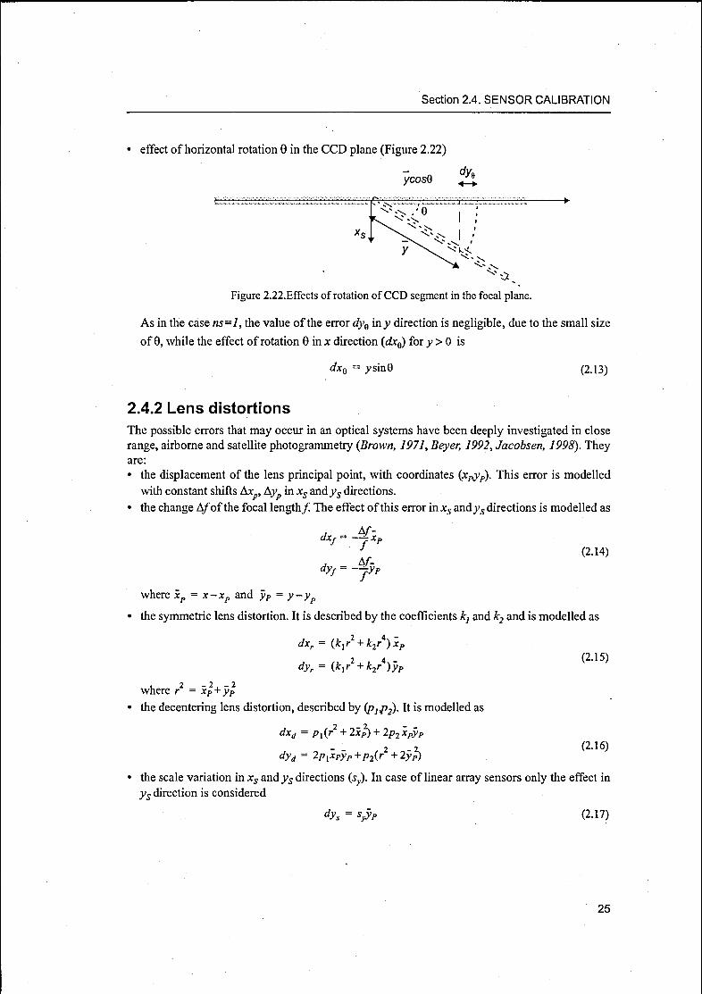
Section 2.4. SENSOR CALIBRATION
effect of horizontal rotation 9 in the CCD plane (Figure 2.22)
ycosQ/e
Figure 2.22.Effects of rotation of CCD segment in the focal plane.
As in the case ns=l, the value of the error dye iny direction is negligible, due to the small size
of 9, while the effect of rotation 9 in x direction (dxQ) for y > 0 is
dxç =
y sind (2.13)
2.4.2 Lens distortions
The possible errors that may occur in an optical systems have been deeply investigated in close
range, airborne and satellite photogrammetry (Brown, 1971, Beyer, 1992, Jacobsen, 1998). Theyare:
• the displacement of the lens principal point, with coordinates (XpyP). This error is modelled
with constant shifts Axp, Ayp in xs andys directions.
• the change Ä/ofthe focal length/ The effect of this error in xs andys directions is modelled as
dxj- = —j xP
if (Z14)
dyf = -
jyP
where xp=
x-xp and yP=
y-yp
• the symmetric lens distortion. It is described by the coefficients kj and k2 and is modelled as
dxr = (kxr + k2r )xP
A tV2+ t S" (115)
dyr = (kxr +k2r )yP
2 2 2where r =
xP + yP
• the decentering lens distortion, described by (pjp2). It is modelled as
dxd= px(r2 + 2xp) + 2p2 xPyP
2-2 (2-16)tyd = ip\*pyp+Pi(r +iyp)
• the scale variation inxs andj>s directions (sy). In case of linear array sensors only the effect in
ys direction is considered
dys = Syjp (2.17)
25

Chapter 2. LINEAR CCD ARRAY SENSORS
2.4.3 Laboratory calibration
High precision photogrammetric cameras require high resolution geometric, spectral and radio¬
metric laboratory calibration. An inaccurate interior orientation would consequently lead to sys¬
tematic errors in the photogrammetric point determination as well as in all follow-up products.For this reason the purpose of geometry laboratory calibration is the precise measurement of
object side image angles for a sufficient number of sensor elements ofeach single CCD array.
In the following, two systems for the laboratory geometric calibration of pushbroom sensors are
briefly reported, one for a spaceborne sensor (MOMS-02) and one for an airborne sensor (Sta-rlmager).The first calibration facility is located at the Institute of Space Sensor Technology at DLR. It was
originally developed for the calibration of spaceborne sensors in the visible range and was latelyextended to the infrared spectrum. This system has been used for the calibration of spacebornesensors like MOMS-02/D2, MOMS-P2 (Kornus etal, 1996), HRSC (Ohlhofand Kornus, 1994),WAOSS-B (Schuster et al, 2002) and the airborne camera ADS40 (Schuster and Braunecker,
2000).The optical system to be calibrated is mounted on a tum-table with two orthogonal rotation axis;the calibration system includes a collimator support oriented along the third orthogonal axis. The
vertical x-axis is pointing in the flight direction and the horizontal jv-axis is directed along the
sensor lines. In an initial zero-position both axes are adjusted approximately perpendicularly to a
reference direction, defined by a Cassegrain collimator. In Figure 2.23 the calibration system for
MOMS-P2 is shown. In the initial zero-position the x-axis, the y-axis and the collimator axis
define an orthogonal cartesian coordinate system. Deviations from orthogonally introduce errors
in the image angle measurements. Referring to Figure 2.24, the errors that can occur are: the non-
orthogonality between x- andy- axes (angle j'), the non-orthogonality between v- and collimator
axes (angle v) and the non-orthogonality between x- and collimator axes (angle a). In order to
compensate for these errors the measurements are carried out in two sequences per set, firstly in
"normal" position, then in "reverse" position (the optical module is rotated 180° around the pr¬
axis and the_y-axis). The mean values of both sequences are free of errors ; and a. Since v is not
estimated in this way, the jc-axis must be carefully adjusted orthogonally to the collimator axis
prior to calibration and never be changed during the entire process. Then v can be determined
from the v-angles measured in normal and reverse position at azimuth angle equal to 0.
From these measurements the camera model parameters and the correction tables can be derived,
describing the relative location of each CCD array and the deviations of the single pixel location
from the camera model. The final values of the single pixel location (xy) are compared againstideal values, which assume a straight horizontal sensor line and constant distances between the
pixel centers. The deviations dx and dy are modelled with linear and parabolic functions depend¬ing on parameters that describe the sensor rotation and curvature, focal length and along-trackdisplacement. These calibration parameters are estimated and used to correct the nominal values
of the sensor rotation and curvature, focal length and along-track displacement. For more details
about this laboratory calibration see Kornus et al, 1996 and Kornus, 1996.
26

Section 2.4. SENSOR CALIBRATION
Turn Tabicß
Illumination
Optics
53
Azimuth
axis
> a
v
;
i
i
i
i
Collimator axis
•*-<x
Figure 2.23.Configuration of calibration equipment at Figure 2.24.Non-orthogonality of
DLR (Kornus et al, 1996). calibration equipment
(Kornus, 1996).
The second example of laboratory geometric calibration is the one for the three-line scanner Sta-
rlmager (SI), by Starlabo Corporation, Tokyo. The sensor optical system consists ofone lens and
9 or 10 CCD lines (depending on the SI version) in the focal plane for the forward, nadir and
backward viewing. The parameters of the interior orientation that are calibrated include the shift
of convergent stereo channels, the offsets of the multispectral line arrays, the focal length and the
lens distortions (Chen et al, 2003). The camera is mounted on the stage of the collimator at the
"zero position" and aligned with regard to the spatial fixed (camera) system with coordinates xy
(Figure 2.23); the center of the entrance pupil coincides with the center of rotation of the stageand the longitudinal axis of the nadir-looking CCD array is parallel to the v-axis and perpendicu¬lar to the x axis. The collimator ray from a pinhole target at the collimator focus passes throughthe TLS camera's lens center at angle a in the y direction and angle ß in the x direction, and is
deformed by lens distortion (Figure 2.24). The distortions Ax, Ay are measured and described bythree unknown parameters for each CCD line (offset of principal point and angle between the
CCD line and the j-axis) and six unknowns for the whole camera (focal length, three parametersfor symmetric distortion, two parameters for tangential distortion). Finally the tables containingthe correct values xy of the position of each detector ofeach CCD array are produced.
Figure 2.25.Geometry scheme for laboratory calibration Figure 2.26.Equipment for laboratory cali-
of Starlmager (Chen et al, 2003). bration of TLS (Chen et al,
2003).
27

Chapter 2. LINEAR CCD ARRAY SENSORS
2.5 STEREO ACQUISITION
CCD linear array sensors can acquire stereo images with two different configurations, across and
along the flight direction, as described in the following paragraphs.
2.5.1 Across-track
In across-track configuration, the CCD lines and the optical system are combined with a mirror
that rotates from one side of the sensor to the other across the flight direction (Figure 2.27). The
along-track angle is constant and close to zero (Figure 2.28). The across-track angle is usually upto 30°, but can reach larger values (for example 45° with Orbview-3). The number of strips is
equal to the number of channels (one for each CCD line), all looking in the same direction. At the
next satellite pass over the area of interest, the strips are acquired with a different viewing angle.
According to this configuration, the stereo images are collected from different orbits, with the
overlapping area across the flight direction (Figure 2.28). Considering a pair of images of the
same area acquired with viewing angles a7 and a2, the base over height ratio is
- = tana1-tana2 (2.18)
The most relevant consequence of this configuration is that the time interval between the acquisi¬tion of two stereo scenes can be in the order of days or more, therefore differences in the land
cover, due to natural events or human actions, and in the cloud distribution may occur.
Figure 2.27.Acquisition with across-track stereo viewing.
The High Resolution Visible (HRV), the High Resolution Visible InfraRed (HRVIR)and the High Resolution Geometric Resolution (HRG) sensors carried on the SPOT con¬
stellation are an example of across-track stereo scanners, with an oblique viewing capability upto ±27° relative to the vertical (Figure 2.27). Today the two HRV instruments are carried on
SPOT-2 (launched in January 1990), the two HRVIR (Figure 2.29) on SPOT-4 (launched in
March 1998), while two HRG are carried on SPOT-5 (launched in May 2002). They indepen¬dently image the Earth in either panchromatic or multispectral mode. In HRV and HRVIR sen¬
sors, the panchromatic channels use an array of6000 detectors, while the multispectral ones have
3000 detectors per spectral band. The nominal pixel size is of 10m in panchromatic images and
20m in multispectral images. In HRG, on the other hand, the panchromatic channels use two
staggered arrays of 12000 pixels each that produce images with an original ground resolution of
5m and 2.5m after postprocessing with Quincunx sampling, as already described in Section
28
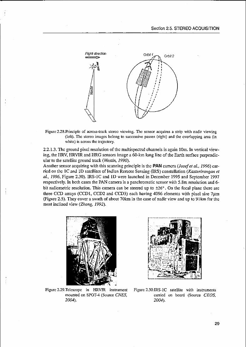
Section 2.5. STEREO ACQUISITION
Flight direction
Figure 2.28.Principle of across-track stereo viewing. The sensor acquires a strip with nadir viewing(left). The stereo images belong to successive passes (right) and the overlapping area (in
white) is across the trajectory.
2.2.1.3. The ground pixel resolution of the multispectral channels is again 10m. In vertical view¬
ing, the HRV, HRVIR and HRG sensors image a 60-km long line of the Earth surface perpendic¬ular to the satellite ground track (Westin, 1990).Another sensor acquiring with this scanning principle is the PAN camera (Josef et al, 1996) car¬
ried on the IC and ID satellites of Indian Remote Sensing (1RS) constellation (Kasturirangan et
al, 1996, Figure 2.30). IRS-1C and ID were launched in December 1995 and September 1997
respectively. In both cases the PAN camera is a panchromatic sensor with 5.8m resolution and 6-
bit radiometric resolution. This camera can be steered up to ±26°. On the focal plane there are
three CCD arrays (CCDl, CCD2 and CCD3) each having 4096 elements with pixel size 7um
(Figure 2.5). They cover a swath of about 70km in the case of nadir view and up to 91km for the
most inclined view (Zhong, 1992).
Figure 2.30.IRS-1C satellite with instruments
carried on board (Source CEOS,
2004).
Figure 2.29.Telescope in HRVIR instrument
mounted on SPOT-4 (Source CNES,
2004).
29

Chapter 2. LINEAR CCD ARRAY SENSORS
2.5.2 Along-track
In case of sensors with along-track stereo capability, the stereo images ofthe same area are taken
along the flight direction, with a time delay in the order of seconds (Figure 2.31). Images
acquired by successive orbits (satellite case) or flight path (airborne case) may have a small over¬
lapping in the across-track direction too. The main advantage of the along-track stereo acquisi¬tion in the same date over the across-track stereo acquisition in different dates is the reduction of
the radiometric image variations (temporal changes, sun illumination, etc.), thus the increase of
the correlation success rate in any image matching process.
This acquisition geometry can be achieved with two different sensor configurations: multi-line
sensors and single-line sensors with synchronous and asynchronous acquisition.
Figure 2.31.Principle of along-track stereo acquisition from multi-line sensors. Each point is scanned
by the n-lines at different times during the same orbit (for satellites, right). The time differ¬
ences between the acquisitions is smaller than with across-track stereo acquisition.
2.5.2.1 Multi-line sensors
A number ofCCD linear arrays view simultaneously in different looking angles along the trajec¬
tory. A point on the terrain is scanned by each line at a different time, as the platform moves. The
imaging system produces strips with overlapping areas along the flight direction. The most com¬
mon configuration is with three lines viewing simultaneously backward, nadir and forward the
viewing direction (Figure 2.32).A large number of three-line sensors for airborne and spaceborne applications have been
designed and developed in Germany, by Daimler-Benz Aerospace AG (DASA), formerly the
MBB GmbH, and by DLR (Deutsche Forschungsanstalt fur Luft- und Raumfahrt - German
Space Agency), often with the consulting by German Universities (University of Munich, Uni¬
versity of Stuttgard, etc.)One of the pioneer of this camera design was Otto Hofmann, who in the mid 70's experimentedto substitute the film-based data acquisition with linear CCDs. As a result, the pushbroom sensor
EOS (Electro-Optical System) was developed for experimental purposes. Then the technology
improved very quickly and new three-line pushbroom systems were soon available. The multi¬
line pushbroom sensors (the major part of them are three-line sensors) developed by DLR and
DASA are briefly described in the following and shown in Figure 2.33.
Digital Photogrammetric Assembly (DPA). It was constructed by DASA for image acqui¬sitions from airplane (Hofmann, 1986); the optical system consists of one lens for panchromaticscenes in three along-tack directions and additional four lenses for multi-spectral images in the
nadir direction. It has been mostly used for testing and applications at DLR and at the Universityof Stuttgard (Fritsch and Hobbie 1997).
30

Section 2.5. STEREO ACQUISITION
Figure 2.32.Geometry of three-line sensors (left) and their image acquisition (right). The overlap¬
ping areas are along the flight direction.
Monocular Electro-Optical Stereo Scanner (MEOSS). It was designed in the mid 80's byLanzl (Lanzl, 1986). MEOSS had a single lens with a focal length of 61.6mm and 3 CCD sensor
arrays. Each CCD array comprised 3236 sensor elements with 10.7um size. After some airborne
test flights, MEOSS was planned to circle the Earth on an Indian satellite. Unfortunately the
camera was lost in a launch failure in 1993. The photogrammetric processing of the data avail¬
able from the airborne test flight in 1986 and 1989 are reported in (Lehner and Gill, 1989),
(Kornus, 1989) and (Heipke et al, 1996).
Modular Optoelectronic Multispectral Scanner (MOMS). The first MOMS sensor
(MOMS-01) was built by DASA and was mounted on the Shuttle PAllet Satellite (SPAS). The
successor MOMS-02 was built by DASA under contract to the Deutsche Agentur für Raumfahr¬
tangelegenheiten (DARA) and DLR. Two versions of this sensor were built. One was flown on
STS-55 during the Spacelab D-2 Mission from April to May 1993 (MOMS-02/D2, Ackermann et
al, 1989, Seige, 1995, Ebner et al, 1992) and the other one on the Russian MIR station duringthe Priroda mission from May 1996 to March 2003 (MOMS-02/P or MOMS-P2, Seige et al,
1998). The optical system ofMOMS consists of 5 lenses, three for the panchromatic stereo view¬
ing (nadir, forward and backward) and two for the multispectral acquisition in nadir viewing. In
Section 6.2 more details about MOMS-02 will be described.
Wide-Angle Optoelectronic Stereo Scanner (WAOSS). It was developed by DLR for the
MARS mission in 1994 and now a new version of WAOSS (WAOSS-B) is carried on BIRD,which is a small satellite flying at a height of 570km over the Earth surface (Oertel et al, 1992).WAOSS-B is a three line sensor with a single-lens optical system and produces panchromatic ste¬
reo images with viewing angles of 0 and 25°. In the BIRD mission it provides images with a
ground resolution of 145m and a swath width of 753km (Schuster et al, 2002).
Wide-Angle Airborne Camera (WAAC). This sensor is the airplane version of WAOSS and
has the same geometry. It was built to test WAOSS before the MARS mission (Eckardt, 1995).
High Resolution Stereo Camera (HRSC). Together with WAOSS, HRSC was developed
by DLR for MARS-94 mission (HRSC, 2004). The design goal of HRSC was to provide highresolution imaging (10m at 250km altitude), high quality stereo imaging (panchromatic, triplestereo concept), multispectral imaging (four narrow band color channels) and multi-phase angle
imaging for photometric investigations (two additional panchromatic channels yielding images at
31

Chapter 2. LINEAR CCD ARRAY SENSORS
five different phase angles together with the nadir and stereo channels). Today a modified version
of the original HRSC is carried on the Mars Express payload developed by ESA. The modifica¬
tion process made the camera fully compliant with the Mars Express interface requirements (lowmass and power consumption). As in the original version, the camera acquires simultaneous
high-resolution panchromatic stereo images in three viewing direction, together with multi-color
and multi-phase imaging of the Martian surface. An additional Super Resolution Channel pro¬
vides frame images imbedded in the basic HRSC swath at five times greater resolution.
High Resolution Stereo Camera Airborne/Airborne Extended (HRSC-A/AX). As in
the case of WAAC, HRSC-A and -AX are the airborne versions of HRSC, designed for photo¬
grammetric and general remote sensing applications. They are very similar to HRSC, but with
smaller dimensions, lower mass, lower power consumption and a more robust design. The
HRSC-A is practically identical in its main structural features and electronics to the system
developed for Mars 96 with some additional peripheral electronics. The camera has been used byDLR for photogrammetric mapping (Wevel et al, 1999). The HRSC-AX is an optoelectronic dig¬ital airborne multispectral stereo scanner with high photogrammetric accuracy and very high spa¬
tial resolution (10cm from 2500m flight altitude). The HRSC-A and -AX systems are mounted
on a Carl Zeiss T-AS stabilizing platform in their in-flight configuration. Easy handling of opera¬
tions is provided by various automatic modes.
Airborne Digital Sensor 40 (ADS40). This airborne sensor has been built up by DLR in col¬
laboration with LH Systems. It acquires panchromatic and multispectral images using 7 CCD
lines mounted on a single focal plane (Sandau and Eckert, 1996). The instrument provides stripsin three viewing directions, which are not the same in all the versions built.
MOMS-02 DPA WAOSS-B
HRSC on Mars Express HRSC-A ADS40
Figure 2.33.Some of the linear array sensors developed at DLR: MOMS-02 (Source MOMS-02,
2004), DPA (Source Fritsch and Stallmann, 2000), WAOSS-B (Source Schuster et
al, 2002), HRSC on Mars Express (Source ESA Mars Express, 2004), HRSC-A
(Source DLR Berlin, 2004), ADS40 (Source LH-Systems, 2004).
32

Section 2.5. STEREO ACQUISITION
Another sensor based on the three-line stereo acquisition was developed in 2000 by Starlabo, in
collaboration with the University of Tokyo. The sensor is called Starlmager (SI), shown in Fig¬ure 2.34, and is normally carried on helicopter (Murai and Matsumoto, 2000). There are three
versions of this sensor: SI-100, SI-250 and SI-290. SI-100 consists of one-lens optical system
(Zeiss Distagon CD with focal length 60mm) and three CCD lines of 10,200 elements each (pixelsize 7pm), scanning in forward (+21.5°), nadir and backward (-21.5°) directions. There are two
configurations for image acquisition. The first one ensures the stereo imaging capability, in
which the three CCD arrays working in the green channels are read out with stereo angles of
21.5°. The second configuration uses the RGB CCD arrays in nadir direction to deliver color
imagery (Grün and Zhang, 2002a). The next version of STARIMAGER, called SI-250, was
manufactured in 2002 (Murai et al, 2003). With the same focal length of SI-100, it acquiresRGB strips with CCD lines of 14,400 detectors with size 5pm. The off-nadir viewing angles are
23° (forward) and -17° (backward). Additionaly, a NIR line acquires with off-nadir angle 17°
(Madani et al, 2004). The last version of Starlmager, SI-290, is similar to SI-250, but with focal
length of93mm and viewing angles of 15° (forward), -23° (backward) for the RGB and -12° for
the NIR (Kocaman, 2005).
Starlmager 3-DAS-1 ALOS-PRISM
Figure 2.34.0ther three-line sensors: Starlmager (Source Starlabo, 2004), 3-DAS-l (Source Wehrli et
al, 2004) and ALOS-PRISM (Source ALOS Project, 2004).
The three-line principle has also been adopted in the family of the 3-DAS-1 airborne cameras,
developed and manufactured by Wehrli Associates and Geosystem during the last decade. The
optical systems consist of three lenses viewing in forward (+26°), nadir and backward (-16°)directions, and the lenses are available in focal lengths of 35mm, 60mm and 100mm. On each
focal plane three sets of CCD lines acquire strips in RGB channels. The possible CCD lines
dimensions are: 3 x 6,000 pixels with size 12pm, 3 x 8,000 pixels with size 8pm and 3 x 14,400
pixels with size 5 urn (Wehrli et al, 2004).
The stereo principle based on simultaneous three-line scanning will be also used in future mis¬
sions. This is the case, for example, ofthe Panchromatic Remote-sensing Instrument for
Stereo Mapping (PRISM) on board the Japanese Advanced Land Observing Satellite (ALOS),that has been developed at the Japan Aerospace Exploration Agency (JAXA) and will be
launched in 2005 from the Japanese H-IIA vehicle (Tadono et al, 2003). The PRISM sensor,
designed and manufactured at Goodrich (Goodrich, 2004), is supposed to acquire triplets with a
ground resolution of 2.5m in panchromatic model, using three separate lenses with viewing
angles 0° and ±24° (Figure 2.34).
Multi-line scanners with a number of lines different from three also exist and are currently oper¬
ational.
33

Chapter 2. LINEAR CCD ARRAY SENSORS
High Resolution Stereoscopy (HRS). This sensor (Figure 2.35a) from CNES is carried on
the latest satellite of SPOT constellation (SPOT-5) and acquires simultaneously two stereo strips,backward and forward the flight direction. Each CCD array contains 12000 detectors, with
ground resolution of 10m (resampled at 5m in along track direction). More details about HRS
and the results obtained by the georeferencing of its imagery will be presented in Section 6.3.
Visible and Near Infrared (VNIR). This instrument (Figure 2.35b) is a component of the
Advanced Spaceborne Thermal Emission and Radiation Radiometer (ASTER), built by NASAand currently mounted on EOS-AMI. Similar to SPOT-5/HRS, the VNIR subsystem consists of
two independent telescopes viewing nadir and backward (-15°) the satellite trajectory(Yamaguchi et al, 1998). The focal plane of the backward looking telescope contains only a sin¬
gle detector array (band 3B). The focal plane of the nadir telescope contains 3 line arrays (bands1,2 and 3N) and uses a dichroic prism and interference filters for spectral separation allowing all
three bands to view the same area simultaneously (ASTER, 2004). The channels 3N and 3B
acquire stereo images in the near infrared. The results obtained by the georeferencing of a ste-
reopair from ASTER-VNIR imagery will be presented in Section 6.4.
Multi-Angle Imaging SpectroRadiometer (MISR). Together with ASTER, MISR is car¬
ried on EOS-AMI platform and acquires images in four different channels (blue, green, red and
near infrared) along nine different symmetric viewing directions, using 36 linear arrays (Figure
2.35c). The spatial resolution is 275m (all channels in nadir direction and red channel in all off-
nadir directions) and 1100m (blue, green and near infrared channels in off-nadir directions), as
described in Diner et al, 1998b. The results obtained by the georeferencing of MISR imagerywill be presented in Section 6.5.
Airborne Multi-angle Imaging SpectroRadiometer (AirMISR). It was derived from the
MISR concept and used for testing before the MISR launch (Figure 2.35d). Today it is used byNASA for photogrammetric mapping (Diner et al, 1998a).
(b) ASTER-VNIR (AirMISR, 2004).
34

Section 2.5. STEREO ACQUISITION
2.5.2.2 Single-line sensors
Single line sensors have the optical system consisting of one lens and acquire one strip using a
single CCD line. They have the ability to rotate on command around their cameras axes and scan
the terrain with specific viewing angles. The acquisition of stereo images of a particular area of
interest is programmed in advance. Thanks to their flexibility, these sensors can be programmedto acquire stereo scenes both across- and along- the flight direction, in two different methods:
synchronously or asynchronously.
Synchronous acquisition mode
The acquisition mode is synchronous if the satellite speed and the scanning speed are equal.Therefore each image line is acquired with the same viewing angle (Figure 2.36a). Sensors that
follow this principles are:
IKONOS-2. IKONOS-1 and IKONOS-2 (Figure 2.37a) are two very high resolution sensors
developed by Spacelmaging, with KODAK telescopes. After the launch failure of IKONOS-1 on
27 April 1999, IKONOS-2 was successfully launched on 24 September 1999 and is still opera¬
tional. IKONOS scenes cover a squared area of 121km2 with a ground resolution of lm (pan¬chromatic) and 4m (multispectral). The large pointing capability (off-nadir viewing up to 60° in
any azimuth) enables the generation of across-track stereoscopy from two different orbits (suchas with SPOT-4/HRV), as well as along-track stereoscopy from the same orbit (such as with
SPOT-5/HRS).
QuickBird-2. QuickBird-2 (Figure 2.37b) is a very high resolution sensor launched by Digital-Globe in October 2001 (Digital Globe et al, 2003). The sensor, developed by Ball Aerospace
(Ball Aerospace, 2004), provides scenes covering squared area of 262km2 with a ground resolu¬
tion of 0.7m (panchromatic) and 3.4m (multispectral). The CCD line contains 27,000 pixels,obtained with a combination of three linear arrays, each of 9,000 pixels. The QuickBird Basic
Stereo Product includes two stereo images collected along-track on the same pass, generally at
30° off-nadir (forward - backward) and within 10° across the ground track, which provides a base
to height ratio of 0.6 to 2.0, with most collections between 0.9 and 1.2.
Orbview-3. Orbview-3 (Figure 2.37c), manufactured by Orbital Sciences Corporation (OSC)
and operated by Orbimage, was launched on 26th June 2003. The sensor provides both one-meter
panchromatic imagery and four-meter multispectral imagery with a swath width of 8km. The sat¬
ellite is operating in a sun-synchronous, near-polar orbit with an orbital inclination of 97.3° at an
altitude of 470km and revisits each location on Earth in less than three days with an ability to
turn from side-to-side up to 45°. The stereo images are acquired along the flight direction.
Rocsat-2. The Taiwanese ROCSAT-2 satellite (Figure 2.37d) developed by the National Space
Programme Office ofTaiwan (NSPO, 2004), was successfully launched on 20 May 2004 and has
the main objective of acquiring images over Taiwan for civilian and scientific purposes. The sat¬
ellite carries on board the Remote Sensing Instrument (RSI), that provides images with a swath
width 24km and a ground resolution of2m in panchromatic mode and 8m in multispectral mode
(RGB and NIR). The satellite's agility enables very rapid pointing (up to ±45°) both along and
across track (Chen and Wu, 2000).
Asynchronous acquisition mode
The acquisition mode is asynchronous if the scanning velocity and the platform velocity are not
the same (Figure 2.36). An example ofpushbroom sensor with asynchronous mode is the Earth
35

Chapter 2. LINEAR CCD ARRAY SENSORS
Resources Observation Satellite (EROS-A), launched by in December 2000 (Figure2.3 7d). The EROS project has been developed by ImageSat International, with the cooperation of
Elop's Elbit (Elop's Elbit, 2004) for the telescope construction. The satellite moves in a faster
ground speed than its rate of imaging, ensuring a longer dwell time to allow more light to reach
the CCD linear array sensor of the imager and therefore to improve the quality of the image. The
sensor bends backwards to take its images in an almost constant, predetermined angular speed,
providing a forward-backward pointing; at the same time it employes the across track pointing
capability (Chen and Teo, 2002). The maximum off-nadir angle is 45° both in along-track and
across-track directions. Each line of the images is acquired with a different viewing angle (Figure
2.37e).
Flight direction Flight direction
(a) (b)
Figure 2.36.Principle of along-track stereo viewing with single lines: (a) synchronous; (b) asynchronous.
2.6 PLATFORMS
CCD linear array sensors can be mounted on terrestrial, airborne and spaceborne platforms. In
this context, airborne and spaceborne platforms are taken into account.
Today a large part of sensors used for Earth observation and production of imagery for mappinguse pushbroom sensors.
Among the airborne acquisitions, the portion occupied by linear scanners is not as large as for
space-based pushbroom scanners, because other acquisition instruments (film cameras, digitalframe cameras, laser scanner) represent an alternative method for airborne photogrammetric
acquisitions. Nevertheless, in the last years airborne pushbroom scanners have been reaching an
operational and production status.
In the next sections, the characteristics of satellite and airborne platforms that will be taken into
account for the sensor modelling are described.
2.6.1 Satellite platformsWith the launch of SPUTNIK-1 on October 4, 1957 the space age began, but it took about 15
years to launch a satellite dedicated to civil spaceborne Earth surface imaging: the ERTS (EarthResources Technology Satellite) spacecraft, later renamed to Landsat-1. The CCD line detector
technology was introduced with MSU-E (Multispectral Scanning Unit-Electronic), that was first
flown on Meteor-Priroda-5 in 1980 and provided a spatial resolution of28m and a swath width of
28km. The spaceborne stereoscopic along-track imaging was introduced by MOMS-02 (ModularOptoelectronic Multispectral Scanner), that was flown in 1993 on the Shuttle STS-55 and in
1996 on the MIR station during Priroda mission (Sandau, 2004).
36

Section 2.6. PLATFORMS
Figure 2.37.Single-hne pushbroom sensors: (a) Ikonos-2 (Source Spacelmaging), (b) Quickbird-2
(Source Ball Aerospace), (c) Orbview-3 (Source Novosti-Kosmonavtiki, 2004), (d) Roc-
sat-2 (Source EADS Astrium, 2004) (e) EROS-Al (Source ImageSat International,
2005).
Today hundreds of satellites fly for Earth observation. Among them, we will provide information
on those satellite platforms that carry linear array sensors for photogrammetric applications.
According to their dimension, the satellites can be classified in small satellites, standard satellites
and space stations.
Standard satellites are some meters large and fly at a height between 400 and 700km on the Earth
surface. If constructed by private companies, they usually carry one instrument only, while if
they are financed by national space agencies, they carry different sensors for specific observa¬
tions. Small satellites are smaller and lighter with a shorter expected life. An example of a small
satellite carrying pushbroom sensors is the Bi-Spectral Infra-Red Detection BIRD by DLR
(Schuster et al, 2002), with three instruments for Earth observations on board: the three-line ste¬
reo camera WAOSS-B (Wide Angle Optoelectronic Stereo Scanner), the optional sensor HORUS
(High Optical Resolution Utility Sensor) for verification tasks and HSRS (Hot Spot Recognition
Sensor) for middle and thermal infrared imagery. For an overview on small satellites see Small
Satellites, 2004. A space station is a manned satellite designed to revolve in a fixed orbit and to
serve as a base for scientific observation and experiments, for refueling spacecraft or for launch¬
ing satellites and missiles. One of the most successful space station was the MIR, launched bythe Soviets on 20* February 1986 and destroyed in March 2001. The station had six docking
37

Chapter 2. LINEAR CCD ARRAY SENSORS
ports for cargo transports, visiting manned spacecraft and expansion modules, designed to be
used as research laboratories and living quarters. Among the sensors carried on board, MOMS-
02/P was one of the first digital satellite sensors to provide continuos stereo-panchromatic and
multispectral imagery for DEM generation and orthophoto production (Müller et al, 2001).Satellite sensors can also be classified according to their operators: large public space agencies,large aerospace companies, space nations. Table 2.1 shows the classification proposed byDenore, 2000.
In general commercial satellites developed by private companies are designed to meet the users'
requirements, in terms of resolution, ready-to-use products and temporal coverage. They usually
provide high or very high resolution imagery for terrain mapping, orthophoto generation and
object extraction. The along-track or across-track stereo acquisition of a particular region of
interest is planned in advance and the satellite can be manoeuvred in order to satisfy as much as
possible the users' stereo requirements. The missions planned by large public space agencies, on
the other hand, have the main objective to provide the users with useful tools for land planningand resource mapping and monitoring. Small satellites, which are cheaper, are usually built by
companies or agencies with a more limited budget and try to fulfill specific requirements (price,
coverage, etc.) which make them competitive with respect to the other image providers.
Table 2.1. Earth resource satellite observing systems (Denore, 2000).
OPERATORSATELLITE
SYSTEM TYPEOBJECTIVE EXAMPLES
Large public spaceagencies
High resolution land
resources
Resource mapping SPOT, Landsat,IRS-1C
Large aerospace
companiesVery high resolution Detailed mapping IKONOS, Quickbird,
EROS-A1
Emerging spacenations, Universitystart-up companies,SME's, etc.
Small-satellites,
medium-high resolu¬
tion
Science
Technology develop¬ment
Industrial policyNational pride, etc.
SunSat, Kitsat, BIRD
2.6.1.1 Orbit characteristics
Satellite orbits have several unique characteristics which are particularly useful for photogram¬metric mapping of the Earth's surface. An orbit cycle is completed when the satellite retraces its
path, passing over the same point on the Earth's surface directly below the satellite (at nadir) for
a second time. The exact length of time of the orbital cycle is called orbital period.Satellite orbits differ in terms of altitude and orientation and rotation relative to the Earth and are
matched to the capability and objectives of the sensor(s) they carry.
For example meteorological and communication satellites have geostationary orbits (Figure2.38) at very high altitudes, approximately 36,000km and revolve at speeds which match the
rotation of the Earth, so they observe and collect information continuously over specific areas.
Due to their high altitude, the geostationary satellites can monitor weather and cloud patterns
covering an entire hemisphere of the Earth.
Usually the platforms that carry pushbroom sensors for photogrammetric mappings fly at lower
heights (300-850km) along near-polar orbits (Figure 2.38). They are designed to follow an orbit
(basically North-South) which, in conjunction with the Earth's rotation (West-East), allows the
sensors to cover most of the Earth's surface over a certain period oftime. A complete coverage of
the Earth's surface is completed after one cycle of orbits. As an example of satellite coverage, in
38

Section 2.6. PLATFORMS
Figure 2.39 the ground track of SPOT constellation is shown.
Apart of near-polar orbits with an inclination near 90°, tilted orbits (inclinations less than 90°)are also possible, but not very frequent (MOMS-02 on MIR platform), because the correspondingEarth coverage is small (Figure 2.38).Most satellite orbits are sun-synchronous such that they cover each area of the world at a con¬
stant local time ofday (local sun time). Therefore at any given latitude, the position of the sun in
the sky as the satellite passes overhead is the same within the same season. As a consequence,
consistent illumination conditions when acquiring images in a specific season over successive
years, or over a particular area over a series of days are ensured. This is an important characteris¬
tic for monitoring changes between multi-temporal image series or for mosaicking adjacent
images together, as they do not have to be corrected for different illumination conditions.
Concerning the physical properties of the orbits, a detailed description will be given in Section
Figure 2.38.Different satellite orbits: a) near-polar; Figure 2.39.Ground track of SPOT orbit with
b) non polar (tilted); c) geostationary. ground receiving stations.
2.6.1.2 List of satellite platforms
Table 2.2 summarizes some information (agency, status, launch date, sensors on board) of the
satellite platforms carrying pushbroom sensors for photogrammetric mapping, together with their
orbit characteristics (height, orbital period, inclination).
39

Chapter 2. LINEAR CCD ARRAY SENSORS
Table 2.2. Main characteristics of satellite platforms. In column STATUS, the following abbreviations
have been used: O for operational, P for not operational, F for future.
SATELLITE AGENCYLAUNCH
DATESTATUS HEIGHT
ORBITAL
PERIOD
(min)
INCLINA¬
TION
(deg)SENSORS
ALOS JAXA end 2005 F 692 99 98.3 AVNIR-2
PALSAR
PRISM
BIRD DLR 22.10.2001 O 570 96 97.8 HORUS
HSRS
WAOSS-B
EOS-AM 1 NASA 18.12.1999 O 705 98.9 98.2 ASTER
CERES
MISR
MODIS
MOPITT
EROS-A1 ImageSatInt
5.12.2000 O 480 94-96 97.3 EROS-A1
IKONOS-2 SpaceImaging
24.9.1999 O 680 98 98.1 lkonos-2
IRS-1C
IRS-1D
ISRO 28.12.1995
29.9.1997
O
O
817
817
101
101
98.6
98.6
PAN
LISS-3
WiFS
J-ERS NASDAa 11.2.1992 O 568 96 97.7 SAR
OPS
MIR DLR 20.2.1986 P 400 89 51.6 MOMS-P2
Orbview-3 Orbimage 26.6.2003 F 480 92.5 97.3 Orbview-3
QuickBird-2 Earth
Watch
18.10.2001 O 450 93.6 97.2 QuickBird-2
Rocsat-2 NSPO of
Taiwan
20.5.2004 O 891 102.8 98.9 RSI
ISUAL
SPOT-1
SPOT-2
SPOT-3
CNES
22.1.1990
P
0
p
832
832
832
101
101
101
98.7
98.7
98.7
2xHRV
Vegetation
SPOT-4 CNES 24.3.1998 0 832 101 98.7 2xHRVIR
Vegetation
SPOT-5 CNES 4.5.2002 o 832 101 98.7 2xHRG
HRS
Vegetation-2
a.now JAXA
40

Section 2.6. PLATFORMS
2.6.2 Airborne and helicopter platformsIn the last decade a large progress in the development of airborne linear array sensors has been
made. These sensors can provide very high resolution and repeated temporal, multispectral and
hyperspectral image data for mapping and GIS applications (Grün et al, 2003b).
Among the pushbroom digital systems used for airborne mapping application we can list: the
MEOSS (Lanzl, 1986), DPA (Müller et al, 1994), the WAAC (Sandau and Eckert, 1996) and the
HRSC-A/AX (Wevel et al, 1999), developed by DLR. As already mentioned, some airborne sen¬
sors were originally designed for simulation of the corresponding satellite-based sensors (for
example WAAC, HRSC-A and AirMISR). Nowadays two commercial airborne sensors are on
the market: the ADS40, by LH-Systems and the Starlmager, by Starlabo. Both systems acquirestrips along three different directions.
Contrary to pushbroom sensors carried on satellite, in the airborne case some sensors have fixed
configurations (for example Starlmager, Figure 2.40) and some others have CCD array configu¬rations different for each camera exemplar, according to the customers requirements. This is the
case ofADS40. Two configurations of this sensor are shown in Figure 2.41.
Viwtfio.-ntheU-s
Flight Di.eßi(M
SÛ&CTi
Figure 2.40.CCD line configuration on Starlmager (Grün and Zhang, 2002b).
+28 »16 0-2 -14 +28 +16 +14 0 -14
II I \ \PANF RGB PANN NIR PANB
/ /\ \ \PANF PANF NIR RGB PANB
Figure 2.41.Two CCD line configurations of ADS40. The numbers represent the viewing angles in
degrees of the corresponding lines below. PANF = panchromatic forward viewing; PANN= panchromatic nadir viewing; PANB = panchromatic backward viewing; NIR = near
infrared; RGB = red-green-blue (Pateraki et al, 2004).
41

Chapter 2. LINEAR CCD ARRAY SENSORS
As airplanes and helicopters do not fly along an accurately predictable trajectory, for the photo¬grammetric point determination the direct measurement of the sensor position and attitude is
required. Therefore GPS and INS instruments are always carried on board. Their observations
are post-processed in order to provide the accurate sensor position and attitude of each imageline. This topic will be investigated in Section 3.1.
Due to the platform instability and vibrations, the original images may be highly disturbed. As
shown in Figure 2.42, the image lines stored one after the other produce straight lines that appear
bent. In this case the sensor position and attitude for each image line are used for the rectification
of the raw images through a projection to a ground plane at a user-specified elevation. The effect
of the rectification is shown in Figure 2.42)
Figure 2.42.Airborne pushbroom imagery before (left) and after (right) rectification. Example with
ADS40 backward images (-14°) over Yokohama, October 2003 (Courtesy of PASCO Corp.).
In case of Starlmager, the pushbroom imaging instruments are mounted together with a stabilizer
to maintain a trajectory with no abrupt changes in position or orientation. In Figure 2.43 the
advantage ofusing a stabilizer is shown.
Figure 2.43.EfTect of stabilizer on pushbroom imagery (Madani et al, 2004).
42

Section 2.7. IMAGE CHARACTERISTICS
2.7 IMAGE CHARACTERISTICS
In the following, the main properties ofthe images acquired by pushbroom sensors are described.
2.7.1 Spatial resolution
The spatial resolution refers to the area on the ground that an imaging system can distinguish. It
is measured as the size of a pixel on the ground, when the image is displayed at full resolution
(CCRS Tutorial, 2004).The ground resolution of satellite imagery is classified as very high (<lm), high (between lm
and 5m), mean (between 5m and 20m), low (between 20m and 50m) and very low (larger than
50m). In the last years this classification has been continuously changing according to the tech¬
nology development. With the successful launch of the EROS-Al, IKONOS-2 and SPOT-5,
imagery with resolution smaller than 5m could be provided for the first time. Quickbird can even
acquire images with less than lm resolution. In the next future, satellite missions carrying very
high and high resolution satellites are planned (Table 2.3).The spatial resolution of passive sensors depends primarily on their Instantaneous Field ofView
(IFOV). The IFOV is the angular cone of visibility of the sensor and determines the area on the
Earth's surface which is 'seen' from a given altitude at one particular moment in time. In the cur¬
rent airborne scanning systems, the IFOV is generally equal to 1.0 ~ 2.0 milliradiants, while in
spaceborne scanning systems the IFOV is smaller than 0.1 milliradiants. Using the IFOV (indi¬cated with the letter a) and according to the geometry shown in Figure 2.44, the length of a pixelon the ground in the CCD line direction (ay) can be calculated with the following formula (Wang,
1990,p.524)
a = = - (2.19)cos g (cosß)
where R is the inclined distance between the object and the sensor, His the flight height and Q is
the scanning angle.The size of a pixel in the flight direction (ax) is usually equal to ay and can be calculated as
a-H (2.20)x
cosg
As expected, the ground pixel size is directly proportional to the platform flying height and to the
IFOV.
For a wider analysis of the relationship between the instrument geometric parameters and the
imagery ground resolution, the orbit characteristics and other factors must be taken into account.
The following formula
ë= tl = ti (2.21)
/ Py Px
shows the dependency of the ground resolution (ax and ay) on the pixel size (px andpy), the focal
length/and the flight height H. By fixing the minimum pixel size to 6 urn, the ground pixel size
is directly proportional to H and inversely proportional tof. This means that for high resolution
sensors (small ax and ay) low orbits and high focal lengths are recommended. Anyway, physicalconstraints for the focal lengths exist and low trajectories have a small swath width, which can be
improved by using more imaging elements in each line or multiple segments in one line. More¬
over if lines with more CCD elements are used, a small ground pixel size cannot be guaranteedalong the full image line (effect of a). The satellite systems combine these parameters in order to
43
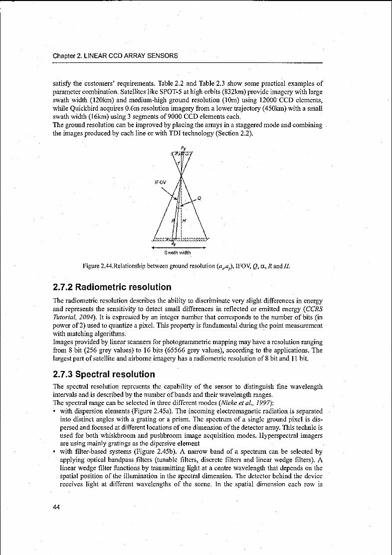
Chapter 2. LINEAR CCD ARRAY SENSORS
satisfy the customers' requirements. Table 2.2 and Table 2.3 show some practical examples of
parameter combination. Satellites like SPOT-5 at high orbits (832km) provide imagery with largeswath width (120km) and medium-high ground resolution (10m) using 12000 CCD elements,while Quickbird acquires 0.6m resolution imagery from a lower trajectory (450km) with a small
swath width (16km) using 3 segments of 9000 CCD elements each.
The ground resolution can be improved by placing the arrays in a staggered mode and combiningthe images produced by each line or with TDI technology (Section 2.2).
Svrath
Figure 2.44.Relationship between ground resolution (a^a^, IFOV, g, a, R and H.
2.7.2 Radiometric resolution
The radiometric resolution describes the ability to discriminate very slight differences in energy
and represents the sensitivity to detect small differences in reflected or emitted energy (CCRSTutorial, 2004). It is expressed by an integer number that corresponds to the number of bits (in
power of 2) used to quantize a pixel. This property is fundamental during the point measurementwith matching algorithms.
Images provided by linear scanners for photogrammetric mapping may have a resolution rangingfrom 8 bit (256 grey values) to 16 bits (65566 grey values), according to the applications. The
largest part of satellite and airborne imagery has a radiometric resolution of 8 bit and 11 bit.
2.7.3 Spectral resolution
The spectral resolution represents the capability of the sensor to distinguish fine wavelengthintervals and is described by the number ofbands and their wavelength ranges.
The spectral range can be selected in three different modes (Nieke et al, 1997):• with dispersion elements (Figure 2.45a). The incoming electromagnetic radiation is separated
into distinct angles with a grating or a prism. The spectrum of a single ground pixel is dis¬
persed and focused at different locations ofone dimension ofthe detector array. This technic is
used for both whiskbroom and pushbroom image acquisition modes. Hyperspectral imagersare using mainly gratings as the dipersive element
• with filter-based systems (Figure 2.45b). A narrow band of a spectrum can be selected by
applying optical bandpass filters (tunable filters, discrete filters and linear wedge filters). A
linear wedge filter functions by transmitting light at a centre wavelength that depends on the
spatial position of the illumination in the spectral dimension. The detector behind the device
receives light at different wavelengths of the scene. In the spatial dimension each row is
44

Section 2.7. IMAGE CHARACTERISTICS
detected by the same wavelength• with Fourier Transform Spectrometers (FTS, Figure 2.45c). Spatial Domain Fourier Trans¬
form Spectrometers use the principle of the monolithic Sagnac interferometer. But unlike a
conventional FTS the spectrometer for Earth observation operates with fixed mirrors. The
optical design distributes the interferogram (spectrum) in one dimension of the detector. The
other dimension of the area array detector corresponds with the swath width.
The most common spectral selection mode for pushbroom sensors is the filter-based one.
Figure 2.45.Three different modes for spectral selection, (a) dispersion element; (b) filter-based sys¬
tems; (c) Fourier Transform Spectrometers (Source Nieke et al, 1997).
CCD linear sensors usually acquire images in panchromatic mode or in multispectral mode (Fig¬ures 2.46 and 2.47). In Table 2.3 the wavelength ranges of the spectral channels used on satellite
and airborne pushbroom sensors are listed.
Advanced multi-spectral sensors for remote sensing applications are the hyperspectral sensors,
which detect hundreds of very narrow spectral bands throughout the visible, near-infrared, and
mid-infrared portions of the electromagnetic spectrum. Their very high spectral resolution facili¬
tates fine discrimination between different targets based on their spectral response in each of the
narrow bands (CCRS Tutorial, 2004).In general the CCD lines corresponding to each channel are placed one parallel to each other in
the focal planes and provide separate strips. The strips for each channel and for each viewingdirections are stored separately. Successively, the user may combine the channels of interest for
specific analysis.In some cases the users are not interested in the single channels, but in the resulting image in true
or false color. In this case the strips, one for each channel, are combined according to different
principles. For example, in case of ADS40 true-color images, during the flight the red, blue and
green arrays are directly optically superimposed in order to generate a color line. This is accom¬
plished with dichroic mirrors, which divide a single light ray into its three color componentswithout significant energy loss, followed by narrow-band filtering to increase the channel separa¬
tion. The great advantage of this approach is that the color image is band registered without sig¬nificant post-processing and thus results instantly in an attractive color picture. In case of
airborne pushbroom imagery, without dichroic mirror arrangement, a high-quality compositefrom three lines with different nadir-offsets would only become available after rectification usinga surface model (Tempelmann et al, 2000).
45

Chapter 2. LINEAR CCD ARRAY SENSORS
Figure 2.46.Multispectral and panchro- Figure 2.47.Multispectral acquisition of MISR sensor,
matic (black lines) acquisi- For each of the nine directions, 4 CCD
tion of ADS40 (Source lines for RGB and NIR channels are stag-
LH-Systems, 2004). gered on the focal plane of the lens lookingin this direction (Source MISR, 2004).
2.7 .4 Temporal resolution
The concept of temporal resolution is usually applied for imagery acquired by satellite systemsinstead of airborne systems. It is linked to the concept of revisit period, which refers to the lengthof time needed by a satellite to complete one entire orbit cycle. The revisit period of a satellite
sensor is usually several days. The absolute temporal resolution of a remote sensing system is the
interval time between two successive acquisitions of the exact same area. In near-polar orbits
(Section 2.6.1.1), areas at high latitudes will be imaged more frequently than the equatorial zone
due to the increasing overlap in adjacent swaths as the orbit paths come closer together near the
poles. Some satellite systems can be manoeuvred and pointed to the target area to reduce the
revisit period. Thus, the actual temporal resolution of a sensor depends on a variety of factors,
including the satellite/sensor capabilities, the swath overlap and the latitude (CCRS Tutorial,
2004).The ability to collect imagery of the same area of the Earth's surface at different periods of time
is one of the most important characteristics of the remote sensors. Spectral characteristics of fea¬
tures may change over time and these changes can be detected by collecting and comparingmulti-temporal imagery. By imaging on a continuing basis at different times we are able to mon¬
itor the changes that take place on the Earth's surface, whether they are naturally occurring (suchas changes in natural vegetation cover or flooding) or induced by humans (such as urban devel¬
opment or deforestation).For photogrammetric mapping applications, a high temporal resolution (small time interval) is
recommended, in order to have small variations between the stereo images. Even with some tens
of seconds delay the cloud cover may quickly change and occlude some parts of the images, as
shown in Figure 2.48.
46

Section 2.8. PROCESSING LEVELS
channel 6 channel 7
Figure 2.48.Example of scene variation due to cloud movement within 40 seconds interval (MOMS-02/P).
2.8 PROCESSING LEVELS
Satellite and airborne images are provided at different processing levels.
Taking into account that each image provider uses a different notation and processing level defi¬
nitions, a general classification of the processing levels is proposed:• Level 0: original data, without radiometric nor geometric processing• Level 1A: radiometrically corrected images. The radiometric calibration coefficients are nec¬
essary for this correction. Usually they are calculated before the flight in laboratory experi¬ments and then systematically in special calibration experiments during the flight period
• Level IB: radiometrically and geometrically corrected images with geometric resampling
(projection on a reference Ellipsoid or on a horizontal plane)• Level 2: ortho-rectified scenes
• Further levels: specific products, according to which applications the sensor is designed for.
For sensors used for photogrammetric mapping these products include the DEM; for other
Earth observation sensors, other products are available; for example, for MISR the MISR 2TC
(MISR Top of atmosphere Cloud retrievals), the MISR 2AS (MISR Aerosol/Surface retriev¬
als) are produced.Usually the pushbroom imagery are available on the market in one of the previous processinglevels. An exception is made by IKONOS scenes, that are not available at the original (raw)level. IKONOS stereo images are distributed in a quasi-epipolar geometry reference where onlythe elevation parallax in the scanner direction remains. For along-track stereoscopy with the
IKONOS orbit, it corresponds roughly to a north-south track, with a few degrees in azimuth
depending upon the across-track component of the total collection angle.For the topic of this research, level 1A images will be used. These scenes have been only radio¬
metrically but not geometrically corrected, therefore a rigorous model that describes their acqui¬sition geometry can be applied for their georeferencing. As a consequence, images like IKONOS
not available at level 1A, can not be oriented with our model.
2.9 LIST OF LINEAR ARRAY SENSORS
The main characteristics of a large number of linear array sensors carried on space- and aircrafts
are summarized in Table 2.3 and Table 2.4 respectively.
47

Chapter 2. LINEAR CCD ARRAY SENSORS
CD CD a> CD CD o CD CD
XI XI X) X> .O T- J3 .a
CO CD <a ro CO CO (0
B/H 1« L_ 'c i_ "C i_ t_
CO JO JO JO JO JO JO> > > > > > >
o o o O o oo ooooo CDo o o o o oo ooooo ro
o in o o CO oo ooooo o
# PIXELS/ csico co CM r- CO-*
CNt-CN CD CD CD CO ^
LINE XCN
CD ,_ 00 ** rr om O oT— T~ CN ^— I^CO CO c~
SWATH
WIDTH (km)
cd •<* *r * * T- >* t T t T-'t'*rf t CN CO CO CO CO 00 in rooog CD
OCNCMCNCN T— CN mT" *"- T_ CN
GROUND CN
RESOLUTIONin
(m)
ooooo ooooo ooooo OOOOO o o OOOOO oOCNOC50 OCOv-CMOO ocMOcno ocNOcno o I-- o)T-cooiio mOJIOCOCDO ojiocor-co otwcdcooj cnmcocoo o> i*- CD CD CD oo r- c-
WAVE- OOOOO ooooo oooino ooooo o o ooooV O
LENGHT (nm)in m cm co co inmtMts m mcMCMco mmcNcocD o CN G)0)t-0)0 o
<*^mcos y^intos ^-"S-m co r-~ t^-iniDN m m * t CD h-COm
m
ZU1ZOK ZIUZOK ZUJZOE ZUJZQüi •7 2 ZZQQiCt: 7
Oujuj^ Oujuj^ <ZDWUJ^ <3WUJ^ < <û.luq;z>
<u. a. LL
cûq; cûq; coq; Cûq; q: w
CHANNELS o CD Ü CD CD
O o m m m ot h- CDCO CD * * •* SI CN CN+l -H +i +i +i +i +1
STEREOo o Q o o o O
ANGLES (deg)a.
3
a.
3
a.3
Q.3
Q.3
Q.
3Q.3
n TO (0
STEREO _l -J Ü
13o _i Ü o
# VIEWING
DIRECTIONSV- CO
FOCAL
LENGHT (mm)
OoCOCO
oooo
oCM00
CN
CDC500
CN
o
oin
CO
oooCN
CNCO
O
CNCO
en
# CAMERAS - - - - - CO - -
Z<
CO a O a.
au
Ö
o
'5
CO
oz
O'>.Q
a:
raV)o
O
<
co
Off
CO
C£a.
co
O
is
o0-
Q
O
co
a O tt UJ < co
48

Section 2.9. LIST OF LINEAR ARRAY SENSORS
B/H 0.5-1.1 0.5-1.1 0.5-1.1 0.5-1.1 1
w
O
-<tco
Ö
CD
dCO
dCO
d
# PIXELS/
LINE
ooooooooooooCO CD CD CD
Ooo
CO
ooo
CN
ooom
TfCOONcocnCOIN
CO
o"3-
*co
m
SWATH
WIDTH (km)
OCD
oCO
oCN
oCO
CD CO CO CO CO COcocommmm
m CO
m
GROUND
RESOLUTION
(m)
OOOOT-CNCNCN
ooooot-CMCMCNCN
ooooo in CO CO CO 00 CO 00 *CNXoo
m
WAVE-
LENGHT (nm)510-730 500-590 610-680 790-890 610-680 500-590 610-680 780-890 1580-1750 490-690 490-610 610-680 790-890 1580-1750 520-600 630-690 760-860
ooininoo(DIOOSCOt-NMnmcoco
i i i i i
oooomoCNCMtCOI-t^lomtmioN
520-600 630-690 760-960 1600-1700 2000-2400 840-900 600-670 840-900
CHANNELS
PAN GREEN RED NIR PAN GREEN RED NIR SWIR PAN GREEN RED NIR SWIR GREEN RED NIR ZZU1ZQCC<C<aujLU5
a. a. _i uj ce"^
mceCD
visible visible NIR NIR NIR ZZZ
Q-Q-Q.
STEREO
ANGLES (deg)
CN
O*-»
ex3
i-~
CN
O*-•
Q.3
oCN+l
o" SId
o-*oooo
CN+1
CO
in
+io"
oinmCM CM+
STEREO o o _l _l _l _j _j
# VIEWINGDIRECTIONS
- T- CN CN CO CM CO
FOCAL
LENGHT (mm)
CNCOo
CMCOO
oCOm
enCNCO
ooooooCD CM CN CN CN CNCDCNCNCNCNCN
m
CM CN
# CAMERAS T— T— CM CM m v- -
X
Si
O0.
CO
cet
1X
Oa.
CO
COa.X
in
Oa.
CO
01
Z
LUV-CO
<
CNa.
co
Sos
COa.
O
toa:LU
m
COCO
O
1
49

Olo
*r—
m> z.
Or-
m73m~
$=tfc
r-2
zXmp ço
O > m co
°.o
3^
3,
71<
Ofn
Oz
co
COH m m O
oço
mrn
co^i
,-^m
Q-O
CD
ta
X > z z m i—
co
H H^
^rn
3'
3,
3ROUND SOLUTION(m)
m ^Hi1
E0S-AM1/MISR
959
9L
0BLUE
GREEN
RED
NIR
443
275-1100
376/1504
Variable
59
±26.1
555
275-1100
376/1504
73
±45.6
670
275
360
1504
95
±60.0
865
275-1100
376/1504
124
±70.5
a.th
isone-lenssensorhastheabilitytorotateandac
quir
estereoimages
up
toacertainoff-nadiran
gle
b.afterresampling
O 3-
CJ
ro
m > 71
O O o > 73 1 03m C/3
O ^303

Section 2.9. LIST OF LINEAR ARRAY SENSORS
D o O CD o •t oooO o o 00 o O oooO * "=r T— o m ooo
# PIXELS/ CN * «t m CM
3
co
COCO CMX Xt-
LINE COCO Xi-COO i_
o
(1)CD 1 CD CD CD CD
C c C C c
CO a.a.
ro co co co
Q. o Q. CL CL CL
PLATFORM< eu
X
o
"5X
< '< < '<
Eo
Eo
<;z
Eo
oo p«to.o
como
r-x§t-r-N
Eo
* o o o ooo o
a13
GROUND
RES.
oCN
0)
m
@in
m
CM
©
COCN
@
m
®CD
(m) CNo
o
o .— *-• o
do. O o
<l>
E
x> O <r <r mincor-o ommo coioomai cocoe»i"~cM co cm oo en * wi-~co
<3 CD z. ^. r-^^mh-o c~mcoco tt mcooo
(3 WAVE- m inin-^dsT moooO
T3LENGHT (nm) CD
•«t00OC0CNOmcoTti^-CM m-a-cor-
"EO
co cf. rrr zuizoo: zco luzdd: UJZDT* z
+
m
z+
m
<3LULU5q._iujq:
<5 IJlULU^-Jince^
3UJLUo + CL -jUJE
a CHANNELS Z CQq: cqq: coq;
Set O
o:CD CD CD CD
oo
co o 00 o> r- OT-coom CD
STEREO 03 co"co
co+i
co+i
coinoocntcoi--
CM
cd"3 i_ CM CM o
o+l +l +i +i
P.
O
CA
O
ANGLES
(deg)§ f- m
i
d
CD
O STEREO < < < < < < <
u
,g # VIEWING
2 DIRECTIONS CO CO CO co C*5 CT> co
TT
CM
FOCAL oS
LENGHT OCO
oco
co
o
mOOC0T
cnencomS mco"co i_y
H (mm) °b
# CAMERAS - - - - - en co
~-co
F §ÊCOMPANY eu
CO>»
co
o
CO
oXI
J2ce ai
<co
CO CO
X_l
(0
Û3co
55_l
Q_i
Q<Z
a> $ a>
5<o
o3 ce
•t o o oco CO
coa
m
CNo
CMt
coce cf s
k.
<
< CO CO X a < eo
co
51

Chapter 2. LINEAR CCD ARRAY SENSORS
2.10 CONCLUSIONS
In this Chapter the geometric acquisition of pushbroom sensors has been investigated. For the
development of a rigorous orientation model for these sensors, these aspects must be taken into
account are:
• the optical system (single or multi-lens) and the lens distortion
• the CCD line design and systematic errors (rotations, shifts and bending in the focal plane)• the integration of internal orientation parameters measured with laboratory calibration
• the platform and therefore the approaches for the external orientation modelling (including the
integration of GPS and INS measurements).
On the market a large variety of imagery at different spatial, temporal, spectral and radiometric
resolutions are potentially available for the users.
The choice of the imagery, including the processing level, depends on different factors:
• applications. This is the main issue. As Figure 2.49 shows, the combination of spatial and
spectral resolutions may provide images with characteristics suitable for specific applications• costs. In general the higher the resolution is, the higher the price is. Additionally, imagery pro¬
vided by private companies are more expensive that imagery provided by national space agen¬
cies
• software availability. For the orientation of pushbroom images suitable algorithms must be
implemented. An alternative is to use commercial software available on the market
• experience.
«3EarthReso irces
beu
a.
AgricultureFoiBstry
o
c>i
X IM Environin2&
rise
"5
S"3
'S
0)
c
C/) s
u
£ak_
u
cTO
a.
^nn/^vsNJJrban
irtationVXy
TopographicMapping
100 m °-1 mo . .
Spatial
10 m
Resolution0J01 m 1m
Figure 2.49.Combination of spectral and spatial resolution for the specific applications (Source
LH-Systems, 2004).
52

3
DIRECT GEOREFERENCING
As seen in Chapter 2, each image acquired by CCD linear array sensors consists of lines indepen¬dently acquired at different times and with a different sensor external orientation (position, atti¬
tude). Today geopositioning systems provide the direct measurement of the sensor position and
attitude at certain instants of time, then accurate interpolation techniques allow the calculation of
the corresponding data at any time and for each image line. Furthermore the satellite trajectoriescan be predicted or simulated by using the physical properties of the satellite orbits. This infor¬
mation, together with suitable interpolating techniques, may be used to calculate the sensor posi¬tion and attitude for the particular instants of acquisition and apply a direct georeferencing.The principle of direct georeferencing is to estimate the ground coordinates of the homologouspoints measured in the images through a forward intersection using as internal orientation the
results of laboratory calibrations (Section 2.4) and as external orientation the data provided bythe geopositioning systems carried on the platform, or the trajectory calculated by mathematical
formulas (only for satellite-based sensors). This approach does not require any ground control
points, except for final checking, and does not estimate any additional parameters modeling the
interior and exterior orientation. For this reason, the effectiveness and reliability of this method
depend on the accuracy of the internal and external orientation data. The alternative approach,called indirect georeferencing and based on the estimation of the sensor orientation through a
bundle adjustment, is treated in Chapter 4.
The sensor model developed for the orientation of pushbroom imagery includes both the direct
and indirect georeferencing approaches. The former is investigated in this Chapter. After the
description of the methods used for the direct measurement of the sensor external orientation
(GPS/INS instruments in Section 3.1 and the analysis of satellite orbits in Section 3.2), the math¬
ematical model for direct georeferencing is presented in Section 3.3. A special attention is paid to
the integration of GPS and INS data into the photogrammetric model (Section 3.4). Finally Sec¬
tion 3.6 will summarize the conclusions on the direct georeferencing approach.
53

Chapter 3. DIRECT GEOREFERENCING
3.1 EXTERNAL ORIENTATION FROM GPS/INS
3.1.1 BackgroundThe traditional way for the georeferencing of spaceborne and airborne imagery is to use groundcontrol points, which represents a big cost for photogrammetric projects. The determination of
the external orientation has always constituted an important topic of the photogrammetric pro¬
cessing. It was Seb. Finsterwalder who, about 90 years ago, called it the fundamental problem of
aerophotogrammetry (Ackermann, 1986). Many attempts have been made in the past to measure
and record the external orientation elements, mostly in aerial photogrammetry applications.Those efforts, however, were not or only partly successful, as the tools were either not accurate
enough or too expensive. Remarkable exception are the statoscope and the APR (Airborne Pro¬
file Recorder), which succeeded in providing accurate vertical camera position or terrain eleva¬
tion data (Ackermann, 1986). Today differential kinematic GPS positioning is a standard tool for
determining the camera exposure centres not only for aerial triangulation (Heipke et al, 2002),but also for satellite positioning. Tests conducted in the last few years demonstrated the quasitotal reduction of GCPs for aerial triangulation, if accurate GPS and INS observations are avail¬
able. The OEEPE test in 2001 showed that direct georeferencing is a serious alternative to classi¬
cal and GPS-assisted bundle adjustment and currently allows for the generation of orthophotosand other products with less stringent accuracy requirements. Few GCPs are essentially only nec¬
essary for calibration, for detecting and eliminating GPS errors such as cycle slips, for reliability
purposes and possibly for datum transformations (see OEEPE test results in 2001, described byHeipke et al, 2001).The importance ofmeasurement systems like GPS and INS is even stronger in case of the georef¬erencing of imagery acquired by pushbroom sensors. In fact with these sensors a bundle adjust¬ment is unrealistic, because the number ofunknown external orientation parameters (six for each
image line!) would be too large. Moreover in case of airborne pushbroom sensors, the aircraft
trajectory cannot be predicted and modelled, as in the satellite case. Therefore the direct mea¬
surement ofthe sensor position and attitude is indispensable.In the next paragraphs, the main principles of the direct measurement of the camera external ori¬
entation with GPS and INS systems are presented.
3.1.2 GPS system2The GPS (Global Positioning System), officially also known as NAVSTAR (Navigation and Sat¬
ellite Timing and Ranging), is part of a satellite-based navigation system developed by the U.S.
Department ofDefense (DoD) and is operational since 27th April 1995.
GPS provides two levels of service: the Standard Positioning Service (SPS) and the Precise Posi¬
tioning Service (PPS). The SPS is a positioning and timing service which is available to all GPS
users on a continuous, worldwide basis with no direct charge, while the PPS is a highly accurate
military positioning, velocity and timing service which is available on a continuous, worldwide
basis to users authorized by the U.S.
The GPS consists of three major segments: space, control and user segment (U.S. Naval Observ¬
atory, 2004). The space segment is a set of satellites providing known locations for resection, the
ground segment is a set ofground control stations that communicate with the satellites and deter¬
mine their locations and the user segment includes all military and civilian users of the system.The segments work together to implement the positioning procedure: the control stations locate
the satellites precisely in space, each satellite generates radio signals that allow a receiver (user)
2. The main reference for this Section is Jekeli, 2001, Chapter 9.
54

Section 3.1. EXTERNAL ORIENTATION FROM GPS/INS
to estimate the satellite location and the distance between the satellite and the receiver; then the
receiver uses those measurements to calculate where on the Earth the user is located.
The space segment consists of 24 operational satellites in six orbital planes (four satellites in
each plane). The orbits are circular with a radius of 20,200km, an inclination angle of 55° and a
period of 12 hour. The position is therefore the same at the same sidereal time each day, i.e. the
satellites appear 4 minutes earlier each day.The control segment consists of five Monitor Stations (Hawaii, Kwajalein, Ascension Island,
Diego Garcia, Colorado Springs), three Ground Antennas, (Ascension Island, Diego Garcia,
Kwajalein) and a Master Control Station (MCS) located at Schriever AFB in Colorado. The
monitor stations passively track all satellites in view, accumulating ranging data. This informa¬
tion is processed at the MCS to determine satellite orbits and to update each satellite's navigation
message. Updated information is transmitted to each satellite via the Ground Antennas.
The user segment consists ofantennas and receivers processors that provide positioning, velocityand precise timing to the user. The receivers contain an antenna that captures signals from visible
satellites, a clock that internally generates signals to synchronize with the incoming satellite sig¬nal and a hardware and software system that process the signals and calculate the receiver's loca¬
tion. The receivers characteristics that can impact the accuracy are: the frequency (single vs.
dual), the number of channels available to track satellites (i.e. how many satellites can be tracked
simultaneously), whether they are differential-ready and whether they use carrier signals in some
fashion. Other receivers characteristics that may influence the choice ofa system with respect to
another one include: the size, the cost, the battery life and the interoperability with other systemslike personal computers.
3.1.2.1 GPS signal
The signal transmitted by the GPS satellites is a carrier wave (sinusoidal) modulated in phase by
binary codes. Mathematically, the signal S(t) (or one component of it) may be represented by
S(t) = AC(t)D(t)cos(2nft) C3-1)
A and/are the amplitude and the frequency of the signal, C(t) is the code sequence, a step func¬
tion having values (1, -1), also known as chips or bits. D(t) represents a data message.
The total GPS signal includes two microwave carrier signals (LI and L2), two code sequences
(C/A and P) and the data message D(t). LI and L2 have frequencies/7 = 1575.42 MHz and,/} =
1227.6 MHz. LI carries the navigation message and the SPS code signals, while L2 is used to
measure the ionospheric delay by PPS equipped receivers.
The two codes that are applied on the microwave carrier signals are (Dana, 2004):• the C/A Code (Coarse Acquisition). It is a repeating 1 MHz Pseudo Random Noise (PRN)Code that modulates the LI carrier signal, "spreading" the spectrum over a 1 MHz bandwidth.
There is a different C/A code PRN for each station vehicle
• the P-Code (Precise), that modulates both the LI and L2 carrier phases. This code is a very
long (seven days), 10 MHz PRN. In the Anti-Spoofing (AS) mode of operation, the P-Code is
encrypted into the Y-Code and requires cryptographic keys for use.
Finally, the Navigation Message (D(t)) modulates the Ll-C/A code signal. The Navigation Mes¬
sage is a 50 Hz signal consisting of data bits that describe the GPS satellite orbits, clock correc¬
tions and other system parameters.The total signal transmitted by a GPS satellite p results
Sp(t) = APPp(t)W"(t)Dp(t)cos(2Kflt)+ AcCp(t)Dp(t)sm(2nflt) + BPPp(t)Wp(t)Dp(t)cos(2nf2t)
55

Chapter 3. DIRECT GEOREFERENCING
C(t) and P(t) represent the C/A and P codes, Ap Ac, and Bp are their amplitudes, D(t) is the data
message and ^represents a special code which is used to decrypt a military code (Jekeli, 2001,
p.263). Due to the spread spectrum characteristic of the signals, the system provides a large mar¬
gin of resistance to interference. Each satellite transmits a navigation message containing its
orbital elements, clock behavior, system time and status messages. In addition, an almanac is also
provided which gives the approximate data for each active satellite. This allows the user set to
find all satellites once the first has been acquired (U.S. Naval Observatory, 2004).
3.1.2.2 GPS observables
At the user segment level, the antenna receives the signal coming from the satellites, recognizesthe satellite (through C/A code) and generates a signal copy. The correlation between the codes
of the incoming and outcoming signals is used for the analysis. The delay of the incoming satel¬
lite codes with respect to the identical codes generated by the receiver represents the time on
transit ofthe satellite codes from the satellite to the receiver. Multiplied by the speed of the light,the resulting distance is not the true range between receiver and satellite, but the pseudorange,because it includes the time lapses due to clock errors, the propagation medium effects, the mul-
tipath and receiver electronic delays. Disregarding these errors, the observed code delay is the
range between the satellite at the point in its orbit when it transmits the signal and the receiver at
the point on the rotating Earth when it receives the signal. The pseudorange is time-tagged by the
receiver clock.
The other type of observable available on all geodetic receivers is the difference between the
phase of the receiver-generated carrier signal at the time of reception and the phase of the satel¬
lite signal at the time of transmission (which arrives at the receiver unaltered except from the
propagation effects that similarly corrupt the code measurement). Since the phases are created bythe clocks, or frequency generators, of the receiver and satellite, the oscillator phase is equivalentto indicated (or tagged) time. As with the pseudoranges, the time interval of transit of the phasesis fraught with errors due to the atmospheric refraction, the multipath, the equipment delays and
the geometric offsets of the phase center from the geometric center of the receiver antenna and
the offset of the satellite antenna from the center of mass.
The largest error is due to the receiver clock. The next significant error source is the medium
where the signal travels: the Ionosphere (between 50 km and 1000 km), which has many free
electrons, and the Troposphere (between the Earth surface and 40 km), which is a non-dispersivemedium with mostly electrically neutral particles. Both effects can be described by suitable phys¬ical models. Other errors in GPS observables include the multipath error (the reflection of the
GPS signal from nearby objects prior to entering the antenna), the equipment delays and biases,the antenna eccentricities (phase center variations) and the thermal noise of the receiver (Jekeli,2001,p.270).
3.1.2.3 Position estimation
The basic principle for position estimation is the measurement of distance between the receiver
and the satellites using a combination of pseudorange and carrier phase observations in order to
remove the constant errors contained in the observations. Some of these errors do not change in
time, such as clock biases and the phase ambiguity, other change more slowly and other have a
long correlation time, such as tropospheric delays. In addition, there are some error terms com¬
mon to different observations that correspond to different receiver-satellite combinations. Usingsimultaneous observations ofpseudorange and carrier phases from several different satellites it is
possible to solve for these and other unknown error terms using an optimal estimation technique,such as a least-squares adjustment. This procedure is known as absolute (point) positioning, since
56

Section 3.1. EXTERNAL ORIENTATION FROM GPS/INS
the position vector of the observer is to be determined from GPS observations independent of
any other point. A more accurate method uses differences between simultaneous observations
from different receivers, thus cancelling the common mode terms and greatly reducing the effect
of some slowly varying error terms. This procedure is known as relative positioning, or differen¬
tial positioning, and yields only the difference in coordinates between two points. If the absolute
coordinates of one point are known, then the relative positioning also yields subsequently the
absolute coordinates of the other point. It is also important to distinguish between static position¬ing and kinematic positioning. As the name implies, static positioning involves placing the
receiver at a fixed location on the Earth and determining the position of that point. Kinematic
positioning, on the other hand, refers to determining the position of a vehicle or platform that is
moving continually with respect to the Earth. This could be attempted either in real time or usu¬
ally with higher accuracy in a post-mission mode. There is an intermediate mode ofpositioning,known as semi-kinematic positioning, whereby the moving receiver (or antenna) is temporarilybrought to rest at those points to be positioned, before moving to the next point, at all times main¬
taining signal lock.
In our case, as the GPS antenna moves with the platform (aircraft or satellite), the processingused for the estimation of the position is a post-mission differential kinematic positioning, also
indicated with the acronym DGPS (Differential GPS).
3.1.3 INS system3The Inertial4 Navigation System (INS) is an instrument for the measurement of linear rates and
linear changes in rates (accelerations) along a given axis. The basic INS consists of an Inertial
Measurement Unit (IMU) or Inertial Reference Unit (IRU), a navigation computer and a clock.
The IMU contains a cluster of sensors (gyroscopes and accelerometers), that are mounted to a
common base to maintain the same relative orientations.
Gyroscopes are instruments that sense angular rate and are used to give the orientation of an
object (angles of roll, pitch and yaw). Rate gyroscopes measure rotation rates, while displace¬ment gyroscopes (also called whole-angle gyroscopes) measure rotation angles.Accelerometers sense a linear change in rate (acceleration) along a given axis. However, theycannot measure gravitational acceleration, that is an accelerometer in free fall or in orbit has no
detectable input. The input axis ofan inertial sensor defines which vector component it measures.
The IMU uses a combination of gyroscopes and accelerometers to maintain an estimate of the
position, velocity, attitude and attitude rates of the vehicle in or on which the INS is carried.
In a typical inertial navigation system, there are three mutually orthogonal gyros and three mutu¬
ally orthogonal accelerometers. This configuration gives three orthogonal acceleration compo¬
nents which can be vectorially summed. Combining the gyro-sensed orientation information with
the summed accelerometer outputs yields the IMU's total acceleration in 3D space. At each time-
step of the system's clock, the navigation computer time integrates this quantity once to get the
body's velocity vector. The velocity vector is then time integrated, yielding the position vector.
These steps are continuously iterated throughout the navigation process.
The inertial navigation systems are classified into two main groups: the gimbaled and the strap-down systems (Figure 3.1). In a gimbaled system the accelerometer triad is rigidly mounted on
the inner gimbal of three gyros. The inner gimbal is isolated from the vehicle rotations and its
3.The main reference for this Section is Grewal et al, 2001, Chapters 2 and 6.
4.Inertia is the propensity of bodies to maintain constant translational and rotational velocity, unless dis¬
turbed by forces or torques, respectively (Newton's first law of motion). An inertial reference frame is a
coordinate frame in which Newton's laws of motion are valid. Inertial reference frames are neither rotatingnor accelerating (Grewal et al, 2001, p.U).
57

Chapter 3. DIRECT GEOREFERENCING
attitude remains constant in a desired orientation in space during the motion of the system. The
gyroscopes on the stable platform are used to sense any rotation ofthe platform and their outputsare used in servo feedback loops with gimbal pivot torque actuators to control the gimbals such
that the platform remains stable. These systems are very accurate, because the sensors can be
designed for very precise measurements in a small measurement range.
A strapdown inertial navigation system uses orthogonal accelerometers and gyro triads rigidlyfixed to the axes of the moving vehicle. The angular motion of the system is continuously mea¬sured using the rate sensors. The accelerometers do not remain stable in space, but follow the
motion of the vehicle.
PIVOTS
SENSOR CLUSTER OF
3 ACCELEROMETERS
3 GYROSCOPES
STABLE
ELEMENT
MOUNTED ON COMMON
RIGID BASE ATTACHED
TO HOST VEHICLE GIMBAL
RINGS
(a) Strapdown (b) Gimbaled
Figure 3.1. Inertial measurement units: strapdown (a) and gimbaled (b) systems (Grewal et al,
2001, p.l2).
As the accuracy concerns, both gyroscopes and accelerometers measurements may contain
errors. The common error sources for gyroscopes are: the output bias, the input axis misalign¬ments, the combined (clustered) three-gyroscope compensation, the input/output non-linearityand the acceleration sensitivity. The main error sources for accelerometers are: the biases, the
parameter instabilities (i.e. turn-on and drift), the centrifugal acceleration effects due to highrotation rates, the center ofpercussion and the angular accelerometer sensitivity.Since there is no single, standard design for an INS, the system-level error sources vary very
much. General error sources can be classified as:
• initialization errors, coming from initial estimates of position and velocity• alignment errors, for the initial alignment of gimbals or attitude direction cosines (for strap-down systems) with respect to navigation axes
• sensor compensation errors, due to the change in the initial sensor calibration over the time
• gravity model errors, that is, the influence of the unknown gravity modeling errors on vehicle
dynamics.
3.1.4 GPS/INS integration5Table 3.1 summarizes the main characteristics of the data provided by GPS and INS systems.GPS offers the possibility to determine position and velocity information at a very high absolute
5. The main reference for this Section is Skaloud, 1999, Chapter 2 and Jekeli, 2001, Chapter 10.3.
58

Section 3.1. EXTERNAL ORIENTATION FROM GPS/INS
accuracy. The accuracy level is dependent on the processing approach (absolute, relative), the
type of observable (pseudorange, doppler, phase measurements) and the actual satellite geome¬
try. To obtain highest accuracy the differential phase observations are used. Solving the ambigu¬ities correctly and assuming a reasonable satellite geometry, a positioning accuracy up to 10cm is
possible for airborne kinematic environments with remote-master receiver separation below
30km. The typical accuracy for the velocity determination is at the level of a few cm/s (Cramer,1999). In contrast to this, inertial systems provide very high relative accuracy for position, veloc¬
ity and attitude information, but the absolute accuracy decreases dependent on runtime if the sys¬
tem is working in stand-alone mode and no external update measurements are available.
Table 3.1. Main characteristics of GPS and INS as precision positioning devices (Jekeli, 2001, p.308).
GPS INS
measurement principle distances from time delays inertial accelerations
system operation reliance on space segment autonomous
output variables positions, time positions, orientation angles
long-wavelength errors low high
short-wavelength errors high low
data rate low (less than 1Hz) high (larger than 25Hz)
instrument cost low ($20,000, geodetic quality) high ($100,000, med/high accuracy)
These contrasting characteristics make GPS and INS systems complementary, rather than com¬
petitive and motivate their integration for precise positioning applications. An optimal integra¬tion allows fully exterior orientation determination with improved overall accuracy and at higherreliability compared to stand-alone units (Cramer et al, 2000b). In fact INS provides directly the
dynamics of the motion between GPS epoch at high temporal resolution, complements the dis¬
crete nature of GPS and aids the positioning solution in the events of cycle slips or losses in the
signal. Table 3.2 summarizes the benefits of GPS/INS integration.
Table 3.2. Benefits ofINS/GPS integration (Skaloud, 1999, p.32).
GPS INS DGPS/INS
high position velocity accu¬
racy over the long term
high position velocity accu¬
racy over the short termhigh position and velocityaccuracy
noisy attitude information
(multiple antenna arrays)accurate attitude information precise attitude determination
uniform accuracy, indepen¬dent oftime
accuracy decreasing with time
low measurement output rate high measurement output rate high data rate
non-autonomous autonomous navigational output duringGPS signal outages
cycle slip and loss of lock no signal outages cycle slip detection and cor¬
rection
not sensitive to gravity affected by gravity gravity vector determination
59

Chapter 3. DIRECT GEOREFERENCING
There are different strategies for the integration ofGPS and INS measurements.
A first distinction is between open and close loops, according as the estimated sensor errors are
fed back to correct the measurements or not. Then the types of integration can be categorized in
two ways:
1. by the extent to which the data from each component aid the other's function (mechanization,architecture of the system). The mechanization is generally related to the concept ofcoupling,that is the degree to which software components/modules depend upon each other (no cou¬
pling implies no data feedback from either instrument to the other for the purpose of improv¬ing its performance). The degree to which components are linked defines whether they
operate in a tightly coupled relationship or in a loosely coupled relationship. Tight coupling is
a form of integration in which each component has knowledge of the other component. The
resulting data are produced simultaneously and optimally and used to enhance the function of
individual sensor components, where possible. Thereby a change in one object will affect the
other object. In loose coupling, one component does not have knowledge of the other and
thereby is insulated from changes in the other. The processed data from one instrument are fed
back in an aiding capacity to improve the utility of the other instruments' performance, but
each instrument still has its own individual data processing algorithm (Hattori et al, 2000). In
case of GPS/INS integration, the real-time feedback of INS velocities to the GPS receiver
enables an accurate prediction of GPS pseudorange and phase at next epoch, thus allowing a
smaller bandwidth of the receiver tracking loop in a high-dynamic environment with a subse¬
quent increase in accuracy. Conversely, inertial navigation improves if the GPS solution func¬
tions as an update in a Kaiman filter estimation of the systematic errors in the inertial sensors.
Similarly, GPS positions and velocities may be used to aid the INS solution in a high-dynamicsituation by providing a better reference for propagating error states based on the linear
approximation.2. by the method of combining or fusing the data to obtain position accuracy. The processing
algorithms for the data combination or fusion may be classified as centralized and decentral¬
ized. Centralized processing are usually associated to tight coupling system integration,because the raw sensor data are combined optimally using one central processor (e.g. Kaiman
filter or smoother) to obtain a position solution. Decentralized processing is a sequentialapproach to processing, where processors of individual systems provide solutions that subse¬
quently are combined with various degrees of optimality by a master processor. In principle,if the statistics of the errors are correctly propagated, the optimal decentralized and central¬
ized methods should yield identical solutions. In some certain cases, such as system fault
detection, isolation and correction capability, the relative computational simplicity makes the
decentralized approach more favorable. As navigation and positioning applications concern,
the centralized approach is considered to yield the best performance, especially since error
statistics can be more rigorously modeled and propagated within the single Kaiman filter
(smoother).
Table 3.3. gives an overview of the advantages and disadvantages of four combined methods for
GPS and INS integration (open loops, closed loops, decentralized loosely coupled and central¬
ized tightly coupled).If properly designed, the closed-loop implementation generally has better performance and is
therefore the preferred implementation when using a strapdown INS. The loosely-coupled filter¬
ing approach has been highly popular due to its modularity and smaller filter size. Although the
arguments for choosing either form of the implementation have been very balanced, the tightly-coupled approach is currently gaining more weight mainly due to the rapid increase in computa¬tional power.
60

Section 3.1. EXTERNAL ORIENTATION FROM GPS/INS
In conclusion, the performance of an integrated INS/DGPS is a complex process depending on a
variety ofparameters including the quality and type of inertial sensors, the baseline length, someoperational aspects, the validity of error models and the estimation algorithm. The improvementsin trajectory determination are usually sought in the development ofbetter models and estimation
algorithms. With the rapid increase of computational power, the trend of finding the most suit¬
able error model for a specific system and specific conditions is being replaced by using a multi-
model approach in conjunction with some type of adaptive estimation. Another limiting factor is
the band frequency. In the lower frequencies, the INS/DGPS integration reduces the overall error
and in the high frequencies, the overall error is not reduced.
Table 3.3. Different forms of Kaiman Filter (KF) implementation (Skaloud, 1999, p.34).
IMPLEMENTATION ADVANTAGES DISADVANTAGES
Open loop • KF may be run external to
INS, suitable for platform INS
• used when only navigationsolution from INS is available
• Non-linear error model due to largesecond-order effect
• Extended KF needed Closed loop
Closed loop • Inertial system errors, linear
model is sufficient
• Suitable for integration at soft¬
ware level
• More complex processing• Blunders in GPS may affect INS
performance
Loosely coupled(decentralized)
• Flexible, modular combination
• Small KF, faster processing• Suitable for parallel process¬
ing
• Sub-optimal performance• Unrealistic covariance
• Four satellites needed for a stable
solution
• INS data not used for ambiguityestimation
Tightly coupled(centralized)
• One error state model
• Optimal solution
• GPS can be used with less
than 4 satellites
• Direct INS aiding throughoutGPS outages
• Faster ambiguity estimation
• Large size of error state model
• More complex processing
3.1.5 Commercial systems
Nowadays different commercial systems are available for the acquisition and integration ofGPSand INS data. They provide the time, position and attitude of the instruments at each time expo¬
sures. Among these systems, the POS/AV by Applanix and the AEROcontrol by IGI mbH (Inge¬nieur-Gesellschaft für Interfaces mbH) are the most used. The potentials of these systems for
direct georeferencing have been also investigated during the OEEPE test "Integrated Sensor Ori¬
entation" (Heipke et al, 2002).
Applanix. Applanix is the company leader in this sector. Its POS/AV system is one of the most
used positioning instrument for photogrammetric applications. According to the data provided in
Applanix, 2004, the accuracy that can be reached with high bandwidth is 0.005° for pitch and
roll, 0.008° in heading (POS/AV 510 - post-processed) and 5-10cm sensor positioning (post-pro¬cessed) at 200Hz data rates. The system is compact, with a lightweight IMU and flexible (differ¬ent post-processing operations can be done in real-time, like differential GPS, time alignment of
airborne sensors and stabilized platforms). For more information, see Applanix, 2004.
61

Chapter 3. DIRECT GEOREFERENCING
AEROcontrol. This system consists of a fibre-optic gyro based IMU and a computer with an
integrated 12-channel L1/L2 GPS receiver.
Depending on GPS constellation and distance from GPS Base/Monitor Station, a positioning
accuracy better than 10cm RMSE and attitude accuracy of 0.01° RMSE for heading and of
0.005° RMSE for roll and pitch can be reached in post-processing. The airborne computer of the
AEROcontrol system is used for data recording of IMU raw data, i.e. angular and acceleration
increments at 64Hz, 128Hz or 256Hz and GPS raw data, i.e. positions and velocities, at 1Hz or
2Hz. For more details, see IGI, 2004.
(a) (b)
Figure 3.2. Two commercial systems for the direct measurement of the position and attitude with GPS
and INS: Applanix POS/AV (left, source Applanix, 2004) and IGI mbH AEROcontrol
(right, source IGI, 2004).
3.2 EXTERNAL ORIENTATION FROM EPHEMERIS
For the imagery acquired by pushbroom sensors carried on satellite, the sensor external orienta¬
tion can be computed from the physical properties of the orbits, through the Keplerian elements,or from the state vectors contained in the ephemeris. In the following paragraphs the calculation
of an approximative sensor external orientation according to two different approaches is
described.
Before going into details, we introduce some reference systems that will be mentioned in the
text: the orbital plane system, the orbit system, the ECl and the ECR.
The orbital plane system (Section B.9) is a two dimensional frame with origin in the focus of the
orbit occupied by the Earth; jc-axis lies on the semi-major axis and points towards the perigee,while they-axis lies in the orbital plane and is perpendicular to x-axis (Figure 3.7).The orbit system (Section B.8), indicated with O, is a right-hand coordinate system with its ori¬
gin at the spacecraft's center ofmass. The z-axis is aligned with the spacecraft-to-Earth pointingvector. The x-axis points along the satellite trajectory, therefore in the direction of the spacecraftvelocity vector. The v-axis is defined by the cross product of the z-axis and the x-axis (Figure3.3).The Earth Centered Inertial system (ECl, Section B.4, Figure 3.4) has the origin in the centre of
gravity of the Earth. The Z-axis points toward the North Pole, the X-axis lies in the equatorialplane and is directed toward the vernal equinox (JR2000), while the Y-axis completes a righthanded orthogonal system (Figure 3.6b).The Earth Centered Reference system (ECR, Section B.5, Figure 3.5) is fixed with respect to the
Earth. The origin is in the centre of gravity of the Earth, the Z-axis points toward the North Pole,the X-axis is the intersection of the plane defined by the prime meridian (Greenwich) and the
equatorial plane and the l^axis completes a right handed orthogonal system.
62

Section 3.2. EXTERNAL ORIENTATION FROM EPHEMERIS
Vernal Equinox
Orbit system*o (0)
*- Y,
Inertial Geocentric
system (I)
Figure 3.3. Orbit system and ECl system.
Greenwich
Meridian
Vernal
equinox
Figure 3.4. ECl system. Figure 3.5. ECR system.
3.2.1 Orientation with Keplerian elements
As mentioned in Section 2.6.1.1, the satellites move along an orbit, whose shape can be
described using the well-known Keplerian elements. According to Keplerian laws, satellites
move in a plane describing an elliptic orbit which can be identified with a set of six orbital
parameters, called snapshot.These six parameters are:
• a (semi-major axis): distance between perigee (point where the satellite is nearest the Earth)and apogee (point where the satellite is furthest from the Earth)
• / (inclination): the angle between the orbital plane and the equatorial plane. By convention,inclination is a number between 0° and 180°
• (0 (argument of perigee): the angle between the nodal line and the semi-major axis, measured
from the ascending node to the perigee. The nodal line is the intersection line between the
orbital plane and the equatorial plane• e (eccentricity): a number between 0 and 1 describing the "shape" of the ellipse: when e is
equal to 0, the ellipse is a circle, when e is very near 1, the ellipse is very long and skinny. It is
calculated as the ratio between the focal distance and the major axis
• F (true anomaly): angle measured in the centre of the ellipse between the perigee and the posi-
63
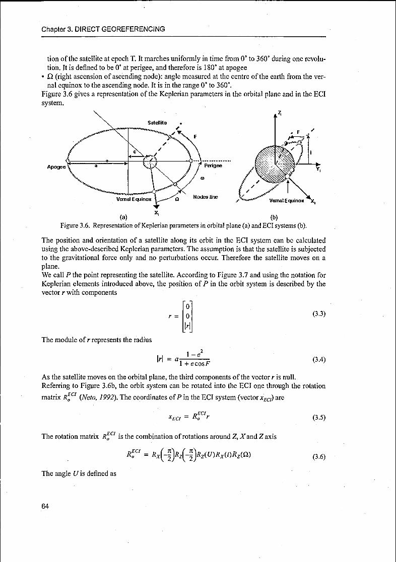
Chapter 3. DIRECT GEOREFERENCING
tion of the satellite at epoch T. It marches uniformly in time from 0° to 360° during one revolu¬
tion. It is defined to be 0° at perigee, and therefore is 180° at apogee• Q (right ascension of ascending node): angle measured at the centre of the earth from the ver¬
nal equinox to the ascending node. It is in the range 0° to 360°.
Figure 3.6 gives a representation of the Keplerian parameters in the orbital plane and in the ECl
system.
Apogee
(a)'
(b)
Figure 3.6. Representation ofKeplerian parameters in orbital plane (a) and ECl systems (b).
The position and orientation of a satellite along its orbit in the ECl system can be calculated
using the above-described Keplerian parameters. The assumption is that the satellite is subjectedto the gravitational force only and no perturbations occur. Therefore the satellite moves on a
plane.We call P the point representing the satellite. According to Figure 3.7 and using the notation for
Keplerian elements introduced above, the position ofP in the orbit system is described by the
vector r with components
r =
The module of r represents the radius
M =a
\-eL
(3.3)
1 +ecosF(3.4)
As the satellite moves on the orbital plane, the third components of the vector r is null.
Referring to Figure 3.6b, the orbit system can be rotated into the ECl one through the rotation
-EClmatrix R0 (Neto, 1992). The coordinates ofP in the ECl system (vector xECI) are
DECI(3.5)
~£C/The rotation matrix R0 is the combination of rotations around Z, Xand Z axis
Ri" = Rx(~)Rz{~)Rz(U)Rx(i)Rz(Çi) (3.6)
The angle Uis defined as
64

Section 3.2. EXTERNAL ORIENTATION FROM EPHEMERIS
U = co + F (3.7)
The complete rotation matrix results
*f'=-sint/-cosQ-sinQ cos/cosf/ -sinQ- sin/
-sinQ -sinU +cosU cosß cos/ sin/ • cosß
sin/- cost/ -cos/
cos £/ • cosß + sinß • cos i • sin U
-sinco -cost/- cosß • cos/ • sinU
-sin/ • sinß
(3.8)
In reality the orbit deviates from the elliptic form due to disturbing non-central forces, that can be
modelled as linear angular changes of F and Q. with time. The principal component of these
forces is the 2nd degree zonal component J2 of the Earth gravitational potential. The first order
perturbations caused by J2 are given by (Kaula, 1966) and are described by
3 J2-n-Reß'= ^ 5--cos(/) + v
2 a -(1-e )
3 J-) • n • R, ?
w'= - - -^ ~ [ 1 - 5 • cos(/)2]
•s2
M'=
4 a2-(1-e2)
3-J2-nR,-(3-cos(i)-l)
~a 2~7I 2.3/24- a (1 -e )
(3.9)
where Re is the Earth's semi-major axis, v is the Earth rotation, n is the mean motion of the satel¬
lite and Mis the mean anomaly.
Satellite
Figure 3.7. Orbital plane system. F is the true anomaly, c the focal distance and r the position vector..
3.2.2 Orientation from state vectors
The ephemeris contain information that varies from one space agency to the other. In general, a
state vector is a set of position, velocity and attitude values for a particular time. The number of
state vectors, the time interval between the observations and the reference systems used are also
varying according to the space agency.
The position, velocity and attitude are usually measured with instruments carried on board. The
star trackers, for example, take an image a region of the sky using a CCD-like optical camera,
and compare successive images to determine how much the orientation of the satellite has
drifted. This information is used by the spacecraft pointing system to determine the actual point¬ing direction of the satellite at any instant. In other satellites, this information is sent to an atti¬
tude control system which then corrects for the drift by using on-board thrusters or other motion-
generating devices to maintain the correct satellite pointing (Image, 2004).
65

Chapter 3. DIRECT GEOREFERENCING
The position and velocity vectors of the satellite contained in the ephemeris are used to calculate
the orientation of the orbital system with respect to the ECl and ECR systems. The difference
between the two frames is that ECl is an inertial system, therefore it does not rotate and is fixed
with respect to the celestial frame. On the other hand, the ECR is fixed with respect to the Earth
frame and is synchronized with the Earth's rotation. In both systems the X- and Y- axes lay on the
equatorial plane and Z is directed along the Earth rotation axis, but in case of ECl system X is
directed toward the vernal equinox (fixed in the celestial frame), while in case ofECR system X
is directed toward the Greenwich meridian (solid for the Earth's rotation). The transformation
between ECl and ECR frames is the following rotation around the Z-axis
= Äz(9)
ECR
(3.10)
ECl
The rotation angle, called 9, is the angle between the meridian of the point P and the meridian
passing by the vernal equinox, or the longitude of P with respect to the vernal equinox. It is
called local sidereal time.
Due to the terrestrial rotation, 9 is time-dependent. According to Figure 3.8, the function 9(/) is
equal to the sum of 9G (longitude of Greenwich meridian with respect to the vernal equinox, or
Greenwich sidereal time) and the latitude \ ofP. It results
Q = QG(t) + XP (3.11)
XP is a constant value, while 9G(r) is a time-dependent function. 9G at time / is calculated adding
the value of 9G at 0h (midnight) of the day of interest and the angular rotation of the Earth
between 0h and t of the day of interest (At). This angular rotation is obtained by multiplying the
Earth's rotation rate (o = 7.29x 10"5 rad/sec with the time Ar in UTC (Coordinated Universal Time)
system. In formulas, it yields
ec(o = ec(o*) + a>,Af (3.12)
6G(0 ) is calculated as
6G(0A) = 24110.54841+8640184.812866-r„ +0.093104-r2-6.2-10"6-r^ (3.13)
where Tu = dJZ6525 and du is the number of days of Universal Time elapsed since JD (Julian
Date) 2451545.0, corresponding to 1st January 2000,12h UT1 (JR2000).After these transformations, the position of the satellite at time t is known in ECR system.
Greenwich
ECl
Figure 3.8. Rotation angles between ECR and ECl systems.
EClThe rotation matrix from the orbit system and the ECl system, indicated with R0 ,
is calculated
66

Section 3.2. EXTERNAL ORIENTATION FROM EPHEMERIS
as (Jovanovic et al, 1999a)
RoCI = [^1^1^] (3.14)
Calling Xj and v7 the position and velocity vectors of the satellite in ECl system (Figure 3.9a), the
vectors r& rç and r^ are calculated with the cross-products of vectors x{ and v7 in this order
(3.15)
rKINI
r<9 =rKxv,
IKxv/1
ro = r<fXrK
^ECR
rK INI
r9 =rK*VG
\h*vG\\
>"<0 = r<?*>*
The same procedure can be applied to calculate the rotation matrix Ra from the orbit system to
the ECR one, using the position and velocity vectors in the ECR system (xG and vG, Figure 3.9b).
Equation 3.15 is modified in
(3.16)
The angles co, cp and K that rotate the orbit system into the ECR system around X, Y and Z can be
calculated by imposing
RE0CR= Rz(k) RY(<?) Rx((o)=
COS9COS& coscosinÂ:+ sin co sin9 cos A: sincusin£-coscusincpcos£
-cosçsinÂr coscocos£- sincosincpsinÂ: sincocosÂ:+ coscosinçsinA: (3-17)
sin9 -sin co cos9 cos ©cos9
with the formulas
co = atan(-—J
(p = asin(rI3) (3,18)
Jt=atan(-^where rtJ is the element ofthe rotation matrix R0CR in row i and columny (Kraus, 1993).
3.2.3 Interpolation between reference lines
In the previous Section we have seen that from the data contained in the ephemeris the values for
the sensor external orientation at particular instants of time can be calculated. The next step is to
interpolate the position and attitude values for the time of acquisition of each line in order to getthe complete set of external orientation parameters for the images. First of all the acquisition time
of each image line is calculated, then the external orientation values are interpolated with cubic
splines.
67

Chapter 3. DIRECT GEOREFERENCING
(a) (b)
Figure 3.9. Calculation of rotation matrix from orbit system to ECl system (a) and ECR system (b).
3.2.3.1 Determination of line time
In general the time of acquisition t, of line i is calculated with a linear interpolation through
Equation 3.19 using the time of acquisition of a line of reference (indicated by the subscript 0)and the integration time (Ats), that is, the time required by the optical system to scan one line on
the ground. In formulas
tt = t0 + (ui-u0)Ats (3.19)
where ut and u0 stand for the row numbers of lines / and 0 in the image and t0 is the time of acqui¬sition of the reference line.
If the integration time Ats is not available, it can be derived using the acquisition time tj and t2 of
two generic lines 1 and 2 in row position ut and u2
3.2.3.2 Interpolation
For the interpolation of the position and attitude, cubic splines are used. The spline functions
belong to the finite elements interpolation methods, which are local (they work step by step on a
single part of the observed data) and very flexible (Crippa and Forlani, 1990). They are defined
on the whole real axis, usually continuos with a suitable (small) number of derivatives, and are
based on simple functions that fit the data points. In particular in cubic splines a series ofuniquecubic polynomials are fitted between each of the data points, with the condition that the curve
obtained is continuous and appear smooth (Figure 3.10). In our application, splines interpolateequally spaced data points, although a more robust form could encompass unequally spacedpoints.The fundamental idea behind cubic spline interpolation is based on the engineer's tool used to
draw smooth curves through a number of points. It consists of weights attached to a flat surface
at the points to be connected. A flexible strip is then bent across each of these weights, resultingin a pleasingly smooth curve. The mathematical spline which is used for the interpolation of theexternal orientation between reference lines is similar in principle. The points, in this case, are
numerical data. The weights are the coefficients on the cubic polynomials used to interpolate the
data. The coefficients "bend" the line so that it passes through each of the data points without any
68

Section 3.2. EXTERNAL ORIENTATION FROM EPHEMERIS
erratic behavior or breaks in continuity. The essential idea is to fit a piecewise function of the
form
S(x) = •
si(x) if xl+x<x2
s2(x) if x2 + x < x3 (3.21)
sn(x) ifxn-l+x<xn
where n is the number ofnumerical data to fit and s, is a third degree polynomial defined by
st(x) = at(x-xt) +bt(x-xt) +cl(x-xl) + di (3.22)
for i=l, 2,..., n-\. The first and second derivatives (s\ and s"t) are
s\ = 3a,(x - x,)2 + 2bt(x - xt) + ct (3.23)
s"i = 6al(x-xl) + 2bi
for i=l, 2,..., «-1.
In order to estimate the coefficients at, bt and ct, the cubic splines must conform to the followingconditions:
1. the piecewise function S(x) interpolates all points2. S(x) is continuos on the interval (jci5 xn)3. S'(x) is continuos on the interval (x}, xn)4. S"(x) is continuos on the interval (xlt x„).
By imposing these conditions on n points and using the notation
y, = S(x,)
Mt = s",(Xi)
h= jrj-x/_j= const
(3.24)
we obtain the matrix equation
1 4 1 0'
00 00
0 14 1 '0000
00 1 4'
0000
0 0 0 0'4 1 0 0
0 0 0 0' 1410
0 0 0 0' 141
Ml
M2
M3
MA
M,B-3
M,n-2
M,n-\
Mm
yx-2y2 + y3
y2-2y3 + y4
ys-iyA+ys
y„-4-2yn_} + yn_2
yn-i-2yn-2 + yn-\
yn-2-2yn-\ + yn
(3.25)
This system with dimension (n-2, n) is under-determined. In order to generate a unique cubic
spline, two other conditions must be imposed upon the system.This leads to the definition of three main types of splines:1. Natural Splines. The second derivative is set equal to zero at the endpoints: Mx = Mn= 0
2. Parabolic Runout Splines. The second derivative at the endpoints M, and Mn, is imposed to be
equal to M2 andM„_j, respectively: Mx - M2andMn = Mn_l.
3. Cubic Runout spline. This type of spline has the most extreme endpoint behavior. It assigns
69

Chapter 3. DIRECT GEOREFERENCING
Mj to be a combination ofM2 and M3 and Mn to be the same combination for Mn_j and Mn_2:
Mi = 2M2-M3 and Mn = 2M„_l-M„_2. This causes the curve to degrade to a single cubic
curve over the last two intervals, rather than two separate functions.
Once all the conditions have been set, the unique solution (polynomial coefficients) can be calcu¬
lated. In all three forms, the cubic splines are especially practical, because the set of equationsimposed not only are linear, but also tridiagonal. Each Mt is coupled only to the nearest neighborsat i 1, therefore the equations can be sol>ed in 0(N) operations (De Boor, 1978).In our case the interpolation of the position and attitude vectors for all the acquisition times is
carried out using natural splines.
Figure 3.1 O.Interpolation with cubic splines (Crippa and Forlani,
3.3 DIRECT GEOREFERENCING
Using the sensor external orientation estimated for each line and any internal orientation parame¬
ters available from laboratory calibration (Section 2.4), the image coordinates of homologouspoints can be transformed in the object system through a forward intersection (direct georefer¬encing). In frame photogrammetry each image is acquired from a separate perspective center and
is therefore the result of a central perspective. On the other hand, in images acquired by pushb¬room sensors, each image line is independently scanned while the sensor is moving along its tra¬
jectory. As a consequence, the perspective projection and the collinearity equations are not valid
for the full image, but in each CCD line direction only.Like in frame photogrammetry, the points are measured in the image and transformed in this
order:
1. from image to camera system, through an affine transformation
2. from camera to object system, based on the collinearity equations.In the second transformation the points must be observed in at least two images and their objectcoordinates are estimated with forward intersection in two steps. In the first one the approxima¬tion of the ground coordinates are calculated by forward intersection of the two most external
images, because the base over height ratio is bigger and the stereoscopy is more favorable (Fig¬ure 3.11a). Once the approximate ground coordinates are known, they are refined with a least
squares solution in the second step, using all the available lines (Figure 3.1 lb).In the next sections, the mentioned reference systems and transformations are described.
3.3.1 From image to camera coordinates
The image system is a 2D system in image space with origin in the top upper-left image pixel andtwo orthogonal axis oriented along the image rows (v) and columns (u), as described in Section
B.l and Figure 3.12a. The image coordinates (u,v) are transformed into the scanline system (indi¬cated with S). This system is defined for each image line and is centered in the mean pixel of the
line, wifhj^ axis parallel to the image line and;c, axis perpendicular toy^, close to the flight direc¬
tion (Section B.2 and Figure 3.12b).Assuming an ideal case without lens distortions and geometric errors ofthe CCD line in the focal
70

Section 3.3. DIRECT GEOREFERENCING
Image 1 Image 3 Image 3
(a) (b)Figure 3.11.Steps of direct georeferencing algorithm for three-line sensors: a) intersection of two
homologous rays and b) refinement with three rays.
plane, the coordinate^ can be calculated with the transformation
*-(v-£>, (3.26)
where py is the pixel dimension iny^ direction and A^, is the number of pixels in each line. The
coordinate xs is fixed equal to zero.
If the pre-flight laboratory calibration results are available, the given exact position of each CCD
line in the focal plane are used as xs andy^ values.
The camera system (indicated with letter C) is a 3D system centered in the perspective center
(PC) of each lens (Section B.3 and Figure 3.12c). The axis xc andyc are parallel to xs andyr The
z-axis zc is upwards directed and completes a right-hand coordinate system. The value of zc is
equal to the lens focal length. The transformation between scanline and camera systems is
y*
-f
(3.27)
Due to the characteristics of the imagery from linear scanners, we cannot define a single camera
system for the full image but we need to suppose one camera system for each line.
0,0
N,R
rows
v At,
columns
Nn
-y.
Flight direction
i
(a) (b)
Figure 3.12.(a) Image system; (b) Scanline system; (c) Camera system.
(c)
71

Chapter 3. DIRECT GEOREFERENCING
3.3.2 From camera to ground coordinates
As each image line is acquired through a central perspective, the relationship between camera
and ground (or object) coordinates can be described by the collinearity principle. This relation¬
ships is valid for each image line.
The object system used for the georeferencing are the local tangential system (Section B.7) for
airborne sensors and the ECR systems (Section B.5) for spaceborne sensors.
For each point observed in the images, the general relationship between camera and ground coor¬
dinates is described by the following equation
(3.28)
where
[X, Y, Z]: point coordinates in the ground system
[Xc, Yc, Zc]: PC position in the ground system
[xc, yc] : point coordinates in the camera system
[xP, yP] : principal point coordinates in the camera system
/: focal length;m: scale factor
i?fcoc?9C)Kc): rotation matrix from camera to ground system.
If the principal point correction is already included in the calibration values, the following equa¬tion is used
X Xc xc xpY = Yc + mR(ac,(pc,Kc) yc-yPZ .Zc_ l-fl
X Xc
Y = YC
z .Zc_
+ 771/?(C0C,CPC,KC)
xc
yc
l-f.
(3.29)
Later or we consider the principal point not included in the calibration values.
Equation 3.28 describes a rototranslation with a scale factor. As shown in Figure 3.14, the vector
[Xc, Yc, Zc] represents the translation from the origin ofthe ground system to the camera PC and
.r?fco09c,Kc) rotates the camera system into a system parallel to the ground one. i?Cco09c,Kc) is
obtained combining three rotations around X, Y and Z, with the attitude angles (cû09c,kc). The
rotation is described by
R((üc, <p0 kc)= Rz(kc) • RY(<pc) Rx(v>c)=
cos9ccoskc coscocsinKc+sincocsin9ccosKc sincucsinKc - coscocsin9ccosKc
-cos9csinKc coscocoskc-sincocsin9csinKc sincocCOSKc + coscocsin9csinKc
sin9c -sincoccos9c coscoccos9c
(3.30)
The external orientation parameters \XC, Yc, Zc, coc, <pc, kc] are different for each image line and
are calculated by GPS/INS measurements or from ephemeris, as described in Sections 3.1 and
3.2.
For sensors whose optical systems consist of more lenses, additional geometric parameters
describing the relative position and attitude of each lens with respect to the nadir one are
imported in the collinearity equations (Ebner et al, 1992). The parameters d , dyJ, dzj represent
72

Section 3.3. DIRECT GEOREFERENCING
the relative position and oc,-, ßy, jj the relative attitude of each lensy with respect to the reference
one (Figure 3.13).
J.'. i
S'A!f['PC,
\ : ^^^rA; °\ d, y°
PC lïc U*J
XrJf A
Figure 3.13.Relative orientation parameters between central line and offnadir line /.
Calling xpj andy^,- the principal point position andfj the focal length of lensy, Equation 4.4 is
extended to
X xc
Y = Yc
A \zc_+ R((ùc, 9C, kc)
xj
yj+ kS((üc, 9C, kc, <Xj, ßy, yj) y-ypj
V-fj\
(3.31)
where
M(Oj, ßy, yj: rotation from camera system of the off-nadir lensy* to camera system of the cen¬
tral lens
R((ù0<p0Kc): rotation from camera system of the central lens to ground frame.
Î = R((£>c, 9C, kc) • M(a,j, ßy, yf;. complete rotation from camera system of the off-nadir lensy
to ground system.
If the relative orientation parameters are equal to zero (nadir case), Equation 3.28 is obtained
from Equation 3.31.
The algorithms that will be presented have been developed both for one-lens and multi-lens CCD
linear sensors. For simplicity, in this Chapter only the formulas for single-lens systems are
reported.
/ZW
Figure 3.14.Transformation from camera to ground systems.
73

Chapter 3. DIRECT GEOREFERENCING
3.3.3 Estimation of approximate ground coordinates
A linear forward intersection of two homologous rays is performed in order to estimate the
ground coordinates that will be used as initial approximations for the least-squares refinement.
It is assumed that the position and the attitude of the sensor projection center is known for each
image line.
The mathematical model is based on Equation 3.28. Calling
~cr
ycr= R((üc, 9c, Kc) (3.32)
Equation 3.28 can be also written as
r ~i p -,
X Xc xcr
Y = Yc + m ycr
z?c_ _Zcr
(3.33)
If point P is measured in two stereo images, we can impose the intersection of the two homolo¬
gous rays (Figure 3.15, yielding
(3.34)
X Xc xcr Xc xcr
Y = Yc + m. ycr= Yc + m2 yCr
Z Zcl zcr Zc 2 zcr
where mt and m2 are the scale factors for the two images. It gives the system
XC\ + m\xcri = XC2 + m2xcr2
Yci+"*iycri = YC2 + m2ycr2
Zcl + mxzcrX = ZC2 + m2zcr2
In matrix notation, we have
xcr\ xcr2m\
Xc2 -Xci
ycn -ycr2*
m-,
— Yc2 ~Yc\
zcr\ ~zcr2_L. -J ZC2 -Zcx
(3.35)
(3.36)
that can be written as
Am = b + e
being e the observation error.
This linear system is solved with linear least squares, with unique solution
T — 1 T
m = (A A) Ab
(3.37)
(3.38)
Substituting the two scale factors contained in vector m into Equation 3.33 for both images, two
different points are indentified in object space. The mean point is taken as approximation (X°, Y
°, Z°) of the ground coordinates ofpoint P.
74

Section 3.3. DIRECT GEOREFERENCING
te*pc,r-«
ac
ïr
w
27PKW
Figure 3.15.Forward intersection with two
3.3.4 Refinement
The ground coordinates (X°, Y°, Z°) are refined using all the available stereo images. The mathe¬
matical model is based on the collinearity equations
ru(X-Xc) + r2l(Y-Yc) + r3l(Z-Zc)= N,Xc J'rn(X-Xc)+r2i(Y-Yc) + r33(Z-Zc) J'D
r2l(X-Xc) + r22(Y-Yc) + r32(Z-Zc)= N^y° J'rn(X-Xc) + r23(Y-Yc) + r3i(Z-Zc) JD
(3.39)
which are obtained solving Equation 3.29 with respect to m. Assuming that point P is observed in
« images, a system containing Equations 3.39 written for each image is formed. The resulting
system contains 2 • n observation equations and three unknown parameters (ground coordinates
of the observed point). The system, which is non-linear with respect to the unknown groundcoordinates, is linearized according to first-order Taylor decomposition using the derivatives:
dx, f ^ = -X(D.12-Vl3)
ox. f ^ = _x(Dr22_V23)
àxe f ,
dÉ= ~^31-^33) || = _X(Dr32_^r33)
D(3.40)
In matrix notation, the linearized system is written as
v = Ad-l
where
(3.41)
A: design matrix, containing the first derivatives of the collinearity functions with respect to
75

Chapter 3. DIRECT GEOREFERENCING
the ground coordinates, evaluated in the approximations (X°, Y°, Z°)d: unknown vector (dX, dY, dZ)v. vector with residuals
/: vector containing the differences between the observed coordinates and the same coordi¬
nates evaluated substituting the approximations in the collinearity equations.
The matrix A is structured as shown in Figure 3.16.
iLSX
ELSX
(a) (b)
Figure 3.16.Structure ofA matrix (a) and derivatives contained in each block (b).
Calling IF the diagonal matrix containing the observation weights, the system is solved with the
solution
image 1
image i 2 rows pr——^i
image n 3 columns
Sx Sx
SY SZ
Sy sy
SY SZ
d = (ATWA) lATWl
The residuals are calculated as
v = Ad-l
and the a-posteriori sigma (ô0 ) is equal to
ao=vTWv
(3.42)
(3.43)
(3.44)
where r is the redundancy of the system (difference between number of equations and the num¬
ber ofunknowns), equal to 2«-3.
The iterations are repeated until all components ofvector d are smaller than a threshold, depend¬ing on the images ground resolution and the accuracy of the point measurement in the images.
3.4 SOME CONSIDERATIONS ON GPS/INS MEASUREMENTS
In case of direct georeferencing with airborne imagery, the ground system is a local tangentialsystem (indicated with letter L), centered at a point O in the study area. In order to use Equation3.28, the angles that rotates the camera system into the ground local system L are needed. Addi¬
tionally the vector containing the camera position from GPS measurement (in ECR system, indi¬
cated with letter G) must be transformed into the local ground system L. Using these systems, the
transformation from the camera system c to the ground local system L is described by
(3.45)
xL Xc xc
YL = Yc + mRLc yc
Zk Zc L-/J
The notation RA represents the rotation matrix from system A to system B. The vector [X0 Y0
Zc] is the camera position given by GPS and transformed in the local ground system L. As the
attitude concerns, the matrix that rotates the camera system in to the ground local one RLC is dif¬
ferent for each line and cannot be directly computed. Taking into account that the measurements
76

Section 3.4. SOME CONSIDERATIONS ON GPS/INS MEASUREMENTS
provided by INS give the rotation angles from the camera system to a local tangential system
(indicated with letter P) centered in the camera PC, Rc is described as the combination of three
rotations: 1. from the camera system c to a local system P (R^), 2. from the local system P to the
ECR one (RP) and 3. from the ECR to the ground local system (RG), as shown in Figure 3.17.
Camera system Platform system<P>
j* Ground local
X system (L)
Geocentric
system (G)
Camera systemy'
z. Platform system
(c) Pc\Ax' <p>
Giound local
y system (L)
* YG
Camera system \ J\ Platform system
Giound local
Cf xL system (L)
z. Platform system(P)
jfH Ground local
V y system (L)
(c) (d)
Figure 3.17.Representation oftransformations: (a) from camera to ground local systems; (b) from camei
to platform systems; (c) from platform to ECR system; (d) from ECR to ground local systei
The matrices are combined in this way
RLc(t) = RLG R°(t) RPc(t)
PC1 L.
Rc and RP are time-dependent, while RG is constant.
(3.46)
Rc is obtained by the rotations of roll (r), pitch (p) and yaw (/') angles (given by INS) around xc,
ycandzc
RPC=cosycosy -cospsiny sin/?
cosrsin/ + sinrsin/?cosy* cosrcosy-sinrsinpsiny -sinrcos/?
sinrsiny- cosrsinpcosy sinrcosy'+cosrsin/jsiny cosrcosp
(3.47)
RG is calculated as
4 = ^(90-9^-^(90-^)
where <pL and XL are the longitude and latitude of the origin ofL system.
(3.48)
77

Chapter 3. DIRECT GEOREFERENCING
C P
Finally, (RP) is the transpose (or inverse) of (RG), defined as
RGP = RPG= Rx(90-<?)-Rz(90-X) (3.49)
where cp and X are the longitude and latitude of the platform, calculated from the GPS measure¬
ments.
This approach is valid if the GPS and INS measurements refer to the camera PC, that is, if the
camera, the GPS and the INS systems are placed in the same position (theoretical case). In prac¬
tise during the georeferencing process, the location of the camera, the GPS and the INS systemsmust be taken into account (Skaloud and Schwarz, 2000, Forlani and Pinto, 2002). Thus we
introduce:
• the GPS local system: tangential local systems with origin in the GPS antenna
• the INS local system: tangential local systems with origin in the INS instrument.
Figure 3.18 shows the mentioned reference systems and their displacements. Using the same
notation as in Equation 3.45, the transformation from camera to ground local coordinates that
takes into account these additional systems, is described by
xL
YL -_
Xc
Yc + RGRpRmsD1NS
mRc
xc
yc
Zk Zc L-/J+ R
INS
GPS
AX,
AY,
AZ,
GPS
GPS
GPS
(3.50)
where
[X0 Ya Zc]: sensor position provided by GPS and transformed to ground local system L
[AXGPS, AYGPS AZGPS\: offset between GPS and camera system
,/MS
Rgps '• rotation matrix from GPS to INS system
RPNS : rotation matrix from INS to local system P.
RrcNS, that rotates the camera system into the INS system, is obtained by substituting the INS
observations into Equation 3.50. The rotation r'gps is calculated according to the angular mis¬
alignments between the GPS and INS systems. The angular and position displacement between
GPS, INS and camera systems should be measured with pre-flight surveying techniques.
GPS SYSTEM
4> ^J^,""*'\p^
<»ns
Figure 3.18.Reference systems used in direct georeferencing with GPS and INS observations.
78

Section 3.5. ACCURACY EVALUATION
3.5 ACCURACY EVALUATION
For the evaluation of the accuracy of the method a sufficient number of Check Points (CPs) are
required. The CPs are measured in the images and in the object space. After applying the direct
georeferencing, the estimated ground coordinates \X Y Z\ of the CPs are compared to the correct
ones [Xcon, Ycorr> Zcorr] and the RMSE are calculated as
Y,(X - XC0J *£{Y- Ycorr) ^(z - ZcoJRMSEX=1-^ RMSEv2 = '-±± RMSE* = ii! (3-51)
n _Cpy
N_CP n_cp
where N CP is the number of CPs.
3.6 CONCLUSIONS
In this Chapter the mathematical formulation of the direct model for the georeferencing of CCD
linear array sensors has been described. The model is based on the forward intersection oftwo or
more homologous rays. The sensor internal orientation must be known, for example from labora¬
tory calibration. For the sensor external orientation, the position and attitude are calculated from
the metadata files of the images and interpolated for each image line with cubic splines. The
accuracy of the method is evaluated throght the RMSE of the check points.For the orientation of pushbroom imagery, the approach based on direct georeferencing is very
powerful because in theory it allows the determination of the ground coordinates of the pointsmeasured in the images without the use ofGCPs, with a considerable reduction of the processingtime, costs and efforts. It is a very useful tool for the evaluation of the accuracy that can be
achieved in the object space using only the information provided by lavoratory calibration and
positioning systems carried on the air- or spacecraft.Other applications based on this approach have also been investigated. For example the algo¬rithm presented in this Chapter has been used for the determination of the ground coordinates of
points measured in Meteosat scenes (Seiz et al, 2004).The results may not be satisfying if the interior orientation parameters, given by pre-flight labo¬
ratory calibration and the exterior orientation measurements are not enough accurate. Anyway,even when those data are available at very high degree of accuracy, additional factors must be
taken into account. For example, if GPS and INS observations are used, the values of the mis¬
alignments and shifts between the positioning and imaging instruments must be known, which is
not always the case. Then few GCPs are needed for the bias corrections, as shown in Poli, 2001.
79

Chapter 3. DIRECT GEOREFERENCING
80

4
INDIRECT GEOREFERENCING
In the previous Chapter we have seen that a possible method for the georeferencing of pushb¬room imagery is to apply a forward intersection using as internal orientation the parameters esti¬
mated in the laboratory calibration and as external orientation the GPS/INS measurements or the
values calculated from the ephemeris (satellite case). We have concluded that the results dependon the accuracy of the point measurements and of the available internal and external orientation.
The alternative method, the indirect georeferencing approach, is used if the sensor internal and
external orientations are not available or not accurate enough for high-precision photogrammet¬ric mapping. According to this approach, the sensor external and internal orientation are esti¬
mated with suitable parameterized functions, together with the ground coordinates of Tie Points
(TPs). The solution is calculated through a bundle adjustment using well distributed GCPs.
In this Chapter the indirect georeferencing model is presented. After the overview of the model
(Section 4.1), the external orientation modelling (Section 4.3), the self-calibration (Section 4.4),the generation of the final observation system (Section 4.5), the solution estimation (Section 4.6)and the accuracy tests (Section 4.7) are explained in details.
4.1 ALGORITHM OVERVIEW
For the georeferencing of CCD linear array sensors the basic collinearity equations represent the
relationship between camera and object systems through a central projection in each image line.
In their standard definition, they are too coarse as mathematical models and cannot describe the
complexity of the pushbroom acquisition geometry. Therefore refinements and extensions of the
equations are required.In order to improve the physical description of the process to be modelled, additional parametersare introduced in the equations and will be determined as part ofthe total adjustment. The choice
ofthe additional parameters must fulfill some requirements. First of all the new parameters must
81

Chapter 4. INDIRECT GEOREFERENCING
not depend on existing parameters to be estimated in the adjustment. Furthermore, if the func¬
tions introduced are polynomials, the degree of the polynomials themselves cannot be too high,in order to avoid the uncontrolled behavior ofhigher degree terms. Statistical methods are useful
to judge how far the individual additional parameters contribute significantly to the modelling.Figure 4.1 shows the development of the proposed algorithm. After extending the collinearity
equations to multi-lens sensors (Section 4.2), the external orientation modelling functions are
introduced and any available GPS/INS information are taken into account (Section 4.3). The sys¬
tematic errors due to the lens and CCD lines distortions are included in the model through a self-
calibration (Section 4.4). Then the resulting system is solved with least-squares adjustment.
COLLINEARITY EQUATIONS FOR ONE-LEN3 SENSORS
EXTENSION TO
MULTI-LENS SENSORS
EXTERNAL ORIENTATION MODELLING
EXTENSION TO GPS/INS
OBSERVATIONS
SELF-CALIBRATION
INTEGRATION IN COLLINEARITY ES.
LEAST SQUARES ADJUSTMENT
Figure 4.1. Scheme of algorithm development.
4.2 EXTENTION TO MULTI-LENS SENSORS
As seen in Chapter 3, for each observed point, the relationship between camera and ground coor¬
dinates (Figure 3.14) is described by
x — xp — —J
y-yP = -f-
rn(X-Xc) + r2X(Y-Yc) + r3X(Z-Zc)
ru(X-Xc) + r23(Y-Yc) + r32(Z-Zc)r2X(X-Xc) + r22(Y-Yc)+r32(Z-Zc)
ru(X-Xc)+r23(Y-Yc)+r33(Z-Zc)
(4.1)
where
[X, Y, Z]: point coordinates in the ground system;
[Xc, Yc, Zc]: PC position in the ground system;
[x, y] : point coordinates in the camera system, wherey is calculated by Equation 3.26 and a: is
equal to zero;
[xp, yP] : principal point coordinates in the camera system;
f: focal length;i?fC0c,cpc'Kc^:rotanori matrix from camera to ground system, with the attitude angles ûJc,<p0Kc-
82
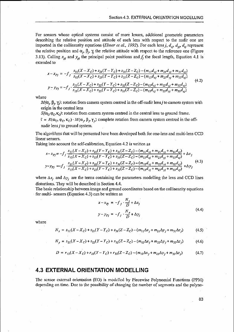
Section 4.3. EXTERNAL ORIENTATION MODELLING
For sensors whose optical systems consist of more lenses, additional geometric parameters
describing the relative position and attitude of each lens with respect to the nadir one are
imported in the collinearity equations (Ebner et al, 1992). For each lensy, dxJ, dyJ, dzj represent
the relative position and a-, ßy, ^ the relative attitude with respect to the reference one (Figure
3.13). Calling xpj and ypj the principal point positions and fj the focal length, Equation 4.1 is
extended to
X-Xp =~fj
sxx(X -Xc) + s2X(Y -Yc) + s3X(Z-Zc)-(mxxdxj + m2xdy) + m3Xdzj)pJ JJ sx3(X-Xc) + s23(Y-Yc) + s33(Z-Zc)-(ml3dxJ + m23dyj + m33dzj)
__,s2X(X- Xc) + s22( Y - Yc) + s32(Z - Zc) - (mX2dxj + m22dvj + m32dzj)
y ypj~ Jj' sX3(X-Xc) + s23(Y- Yc) + s33(Z-Zc)-(mx3dxj + m23dyj + m33dzJ)
(4.2)
where
Mfctj, ßj, yj: rotation from camera system centred in the off-nadir lensy to camera system with
origin in the central lens
S((û0 <Pc>Kc^ rotation from camera system centred in the central lens to ground frame.
? = R((oc, 9C> Kc) " M(aj> ß;> Yp- complete rotation from camera system centred in the off-
nadir lensy to ground system.
The algorithms that will be presented have been developed both for one-lens and multi-lens CCD
linear sensors.
Taking into account the self-calibration, Equation 4.2 is written as
__, sn(X-Xc)+s2X(Y-Yc)+s3X(Z-Zc)-(mxxdXJ+m2Xdvj + m3Xdzj)X XpJ JJ'sx3(X-Xc)+s23(Y-Yc) + s33(Z-Zc)-(mX3dXJ+m23dyJ + m33dzj)
*'
s2X(X- Xc) + s22( Y - Yc) + s32(Z - Zc) - (ml2dxj + m22dvj + m32dzj)(4-3)
y ïpJ JJ 'sx3(X-Xc) + s23(Y-Yc)+s33(Z-Zc)-(mX3dxJ + m23dyJ + m33dZJ)+ y*
where Axj and Ayj are the terms containing the parameters modelling the lens and CCD lines
distortions. They will be described in Section 4.4.
The basic relationship between image and ground coordinates based on the collinearity equationsfor multi- sensors (Equation 4.3) can be written as
x-xpj = -fr — + AXjN
~D
N
y-yPJ = -fj '•£ + Av;(4.4)
where
Nx = sxx(X-Xc) + s2x(Y-Yc) + s3l(Z-Zc)-(mlxAxj + m2XAyj + m3XAzj) (4.5)
Ny = s2X(X-Xc) + s22(Y- Yc) + s32(Z- Zc) - (mx2Axj + m22Ayj + m32Azj) (4.6)
D = rx3(X-Xc)+r23(Y-Yc) + r33(Z-Zc)-(ml3AXj + m23Ayj + m33AZj) (4.7)
4.3 EXTERNAL ORIENTATION MODELLING
The sensor external orientation (EO) is modelled by Piecewise Polynomial Functions (PPM)depending on time. Due to the possibility of changing the number of segments and the polyno-
83

Chapter 4. INDIRECT GEOREFERENCING
mial degree, this function results quite flexible and applicable to both satellite and airplanes tra¬
jectories, as shown in Kratky, 1989, Valadan Zoej and Foomani, 1999 and Grün and Zhang,2002a. Ifone segment only is used, the PPM becomes a parabolic function (Figure 4.2).The platform trajectory is divided into segments according to the number and distribution of
available GCPs and TPs. For each segment **, with time extremes fj^and tlfîn, the variable 1 is
defined as
t =
t-t,
in l
J i (4.8)
lfin~linl
where t is the time ofacquisition of a generic image line.
Then in each segment the sensor external orientation [Xc, Y0 Zc, gjc, cp0 kc] is modelled with
second-order polynomials depending on I
Xc(t) = xl0 + x[t+x2t2
Yc(t) = Yi0 + Y[t + Yi2t2
Zc(t) = z'0 + Z[t+Z2t2
(ùc(t) = coô + (ù[t + (al2t2
9c(0 = 9Ô + (Pi? + <p2?2
Kc(t) = Ki0 + K[t+Ki2t2
[X0, Xj, X2,..., K0, Kj, k2]' are the parameters modelling the external orientation in segment /. At
the points of conjunction between adjacent segments, constraints on the zero, first and second
order continuity are imposed on the trajectory functions: we force that the values of the functions
and their first and second derivatives computed in two neighboring segments are equal at the seg¬
ments boundaries (Section 4.3.2).
Function to be modelled
Segment 1 Segment /' Segment n
lfin
-> time
Figure 4.2. Trajectory modelling with piecewise polynomials.
4.3.1 Integration of GPS/INS observations
In Chapter 4 we have seen that in case ofpushbroom sensors carried on airplane the direct mea¬
surement of the sensor position and attitude with GPS and INS instruments is required, because
the trajectory is not completely predictable.We have also concluded that the observations provided by GPS and INS and filtered with Kai¬
man filter may not be optimal for high-precision direct georeferencing. First of all the observa¬
tions refer to the GPS antenna and the INS instrument, not to the sensor perspective center (asrequired in the collinearity conditions); the offsets and boresight angles between the GPS, INS
and camera systems, if not known or not accurate enough, should be imported in the collinearity
84

Section 4.3. EXTERNAL ORIENTATION MODELLING
equations, estimated and removed from the observations. Another important aspect to take into
account is that the observations may contain residual systematic errors that were not eliminated
in the filtering procedures. For these reasons the external orientation modelling must be extended
in order to integrate and correct the GPS and INS observations. The PPM is suitable for this
extension, as already proved in Grün and Zhang, 2002a. In fact the constant terms (parameters in
Equation 4.9 indicated with subscript 0) can be used for the description of the constant misalign¬ment and boresight angles between the GPS, INS and camera systems, while the first and second
order terms (parameters in Equation 4.9 indicated with subscribes 1 and 2 respectively) may
model other systematic errors occurring in the observations.
The trajectory is again divided into segments and for each segment /, with time extremes t\ni and
tßn, the variable t is defined as
-
_
t-hnt (4-10)
tfiirhm
where t is the time of acquisition ofeach processed line. Ifthe sensor position and attitude obser¬
vations are provided for each line, the line number can be used instead of the time
t =
ini (4.11)
lfln lini
where /Jn<and fß„ are the line extremes of segment /.
The sensor attitude and position of each image line / belonging to segment /, indicated with [Xc,
Yc, Z0 <û0 9c> Kcl/> are modelled as the sum of the measured position and attitude data for that
line [Xinst* Yinst» zinst* «W <(W ^instrl Plus the second order polynomial functions depending on
7, resulting in
xc(t) = xi„str + xi+x[i + xi2i2
Yc(i) = Y^+Y^+Yit + Y^t2
zc(t) = zinslr + zi0 + z[t+zi2t2i t- i-2 (4.12)
<Pc(0 = <IW + <l>o + 9i'" + <p2r'2
*c(0 = K^r + Krj + KlF + K^2
[X0,Xj,X2,..., K0, K/s k2]' are the 18 parameters modelling the misalignment and systematic errors
contained in the observations in segment /. The constant terms [X0, Y0, Z0, co0, q>0, k0](- compensatethe shifts and angular drifts between the image system and the GPS and INS systems, while the
linear and quadratic terms [Xt, Y,, Z;, co/s (p;, K7] and [X2, Y2, Z2, (ü2, (p2, kJ(. model the additional
systematic errors contained in the GPS and INS measurements.
At the points ofconjunction between adjacent segments, constraints for the zero, first and second
order continuity are imposed on the trajectory functions: we force that the values ofthe functions
and their first and second derivatives computed in two neighboring segments are equal at the seg¬
ments boundaries.
85

Chapter 4. INDIRECT GEOREFERENCING
4.3.2 Function continuityThe continuity of the external orientation functions, together with their first and second order
derivatives, are imposed at the points ofjunction between segments.
4.3.2.1 Zero-order continuity
At the point on the border between segment i and i+1, t = 1 in segment i and t = 0 in segment
i+1. Applying the zero order continuity for Xc function, we impose
X'c\ = Xlcl\ (4.13)H( = i
c l/ = o
According to Equation 4.9, we obtain
Xi + X'j+Xit2] =Xi0+l + Xix+lt+x'2+li2\ (4.14)0 1 2
17 = 1° * 2 I? = 0
It yields to
Xi0 + x[+Xt2 = Xi0+l (4-15)
For all the external orientation functions it results
X0 + Xx + X2 = X0
n+ri+^ = z^+i
^n + Zi + Z.^ — Zn
col + 0)', + CO, = coÂ+1
9o + 9i + 92 = 9Ô+1
K0 + Kj + K2 = K0
(4.16)
In case of GPS/INS integration, according to Equation 4.12, we introduce x{l"tr for l'ß„ and
x'"Jstr for l'M. Equation 4.15 becomes
xttr +A +A+X^xZl +X^ (4.17)
As xß",r = X'toltr, the two terms can be cancelled and Equation 4.16 can be used also in case of
GPS/INS observations.
4.3.2.2 First order continuity
We impose that the value of the first derivative of each function at the end of segment i (t = 1 )is equal to the value of the first derivative of the same function at the beginning of segment i+1
(t = 0). In case ofX,-( 7 )
8X'fdt
that is
sxc+1
,- = ,5<
(4.18)
? = o
86

Section 4.3. EXTERNAL ORIENTATION MODELLING
X[ + 2X2t I = x!+1 + 2X2M 11
After substituting t, we obtain'
X[ + 2X2 = X[+ 1
Extending to the other external orientation functions, it yields
X\ + 2X2 = X\+i
y'x + 2Y'2 = y[+1
Z\ + 2Z2 = Z[+1
co1! + 2co2 = cûi+'
9i + 2cp2 = 9i+1
k'1 + 2k2 = k'1+1
(4.19)
(4.20)
(4.21)
Equations 4.21 are also valid in case of GPS and INS integration, because the terms [Xlt
Zinst,-> <*W «Pub». k<«J/ are constant with null derivatives.
Y-
4.3.2.3 Second order continuity
The continuity of the second derivative between adjacent segments is imposed. For function Xc,between segments i and i+1 we have
s2xc
5F2
S2Xc+1
i = ier
7 = 0
(4.22)
that is
2Xi\17 = 1
= 2X.i+\\
17 = 0(4.23)
After substituting t, we get
/Vi — .At (4.24)
Extending to the other external orientation functions, we obtain
vi_
vi+l.A 2
—-" 2
vl-
vi+l
I2- I2
7i _
7i+l
Z2-
z.2
I i+1
C02 = co2
i i+\
92 = 92
-<+l
(4.25)
TC^ — tQ'y
Similar to the first order continuity constraints, Equations 4.25 are valid also in case of GPS and
INS integration, because the constant terms [Ximtl, Yinst„ Zinst„ (ùinstl, q>teû, Kinslr], have null deriva¬
tives.
87

Chapter 4. INDIRECT GEOREFERENCING
4.3.3 Reduction of polynomial order
The degree ofthe polynomial functions modelling the external orientation can be reduced. In fact
all the PPM parameters can be fixed to suitable values. An interesting application is that by fix¬
ing the 2nd order parameters to zero, the polynomial degree is reduced to 1 and linear functions,instead of quadratic functions, are obtained.
This option allows the modeling ofthe sensor position and/or attitude in the segments with 2nd or
1st order polynomials, according to the characteristics of the trajectory.
4.4 SELF-CALIBRATION
The self-calibration is used to correct the observations from systematic errors due to the imaginginstrument. In Section 2.4 we have seen that various errors may occur in the geometry of the
CCD arrays and in the optical system. The most significant errors are modelled with suitable
functions depending on the so-called additional parameters (APs). Further investigation on the
parameters' determinability will indicate which parameters can be estimated. The APs are intro¬
duced in the basic collinearity equations (Equation 4.2) through the Ax and Ay terms (Equation4.3).For the mathematical description of Ax and Av two cases are distinguished: single-lens opticalsystems and multi-lens optical systems.
Single-lens optical systems. We have one lens, one principal point with coordinates (xpyP)in the camera system, one focal plane and NJLINES linear arrays placed on the focal plane. In
this configuration we model the distortion of one lens and the displacement of NJLINES linear
arrays. The additional parameters introduced are:
• Axc and Avc (one set for each CCD line): the displacement ofeach line in the focal plane (Fig¬
ures 2.16 and 2.17)• kj, k2 andpj,p2: the symmetric radial and decentering lens distortions, which are modelled with
Equations 2.15 and 2.16
•
sy: scale factor in y direction, modelled with Equation 2.17
• angle 9 (one for each CCD line): CCD line rotation in the focal plane (Figure 2.18). For small
angles the effect in v direction is neglectable and the one in x direction is modelled with Equa¬tion 2.8.
The total number ofadditional parameters is equal to 5 + NJLINES x 3. The contribution of each
additional parameter is summed. Finally for each liney, the equations that describe the internal
errors are
Axj = AxCJ—jrXP+(kxr +k2r )xP+ px(r + 2xp) + 2p2xPyP+ xPsmQ
Av; = AyCj--LyP + (kxr2 + k2r4)yP + 2plxPJyP + p2(r2 + 2yPl) + syyP
— 2—2—2where xp = x-xp,yP =
y-yp and r = xP + yP.
Multi-lens optical systems. We have NJLENS lenses and one set of CCD line in each focal
plane. In this configuration we model the distortions ofNJ.ENS lenses and the displacements of
NJLINES linear arrays. As we work with 8-bit images (one channel), we consider one CCD arrayin each focal plane, therefore NJLINES=NJLENS. Then the additional parameters modelling the
internal errors are:
88

Section 4.5. OBSERVATION EQUATIONS
• Axp and AyP (one set for each lens): the displacement of the lens principal point. These param¬
eters are perfectly correlated with the displacement of the CCD line in the focal plane (Axc and
Ayc) and include their effect
• kj, k2 andp[,p2 (one set for each lens): the symmetric radial and decentering lens distortion,
which are modelled with Equations 2.15 and 2.16
•
sy (one for each lens): scale factor in y direction, modelled with Equation 2.17
• angle 6 (one for each CCD line): CCD line rotation in the focal plane (Figure 2.18). As for the
single-lens case for small angles, the effect in y direction is neglectable and the one in x direc¬
tion is modelled with Equation 2.8.
The total number of additional parameters is equal to NJLENS x 8. By summing the contribu¬
tions of the additional parameters, we obtain for each lensy
Axj = AxP]- -jxpj+ (kXJr2 + k2jr))xpJ + pXJ(r) + 2xpj) + 2p2jxpj yPJ+ xpJ sinG
Af 2 4 2 2<4-27>
Ayj =
AyPJ~-jr yPJ + (kXjrj + k2Jrf)yP} + 2pXJxpjyPJ + p2j(rj + 2yp.) + syJyPj
where xpj = x-xpJ,yPj = y- ypj and r = xPJ + yPJ.
4.5 OBSERVATION EQUATIONS
In this Section, the observation equations that will form the final system are listed and described.
In the following Equations the observed quantities are overlined and the adjusted orientation val¬
ues are not overlined.
4.5.1 Image coordinates
The coordinates of the GCPs and TPs are measured (=observed) in the images. Their observation
equations are the collinearity equations (Equation 4.4), which describe the relationship between
the observed image coordinates x and y, together with their corrections vx and Vy, and the sensor
external and internal orientation parameters and the ground coordinates of the points
Nxx + vx = x = xPj -fj • — + Ax
N(4-28)
y + vy= y = ypj-fj.-J! + Ay
These equations are not linear. Their linearisation for the adjustment will be treated in Section
4.6.2. The weights given to these observation depend on the accuracy of the measurements,
according to Equation 4.42.
4.5.2 External orientation parameters
Two groups of observations are written for the external orientation parameters. The first group
contains the constraints on the continuity of the PPM functions. To the second group belong the
weighted observations that fix the initial approximations of the PPM parameters to suitable
(observed) quantities.
89

Chapter 4. INDIRECT GEOREFERENCING
4.5.2.1 Continuity constraints
The constraints on the continuity of the PPM functions and their first and second derivatives,described in Section 4.5.2.1, are imported in the equation system as pseudo-observations with
very high weight. As the functions continuity concerns, Equations 4.16,4.21 and 4.25 become
(4 + jri + 4-4+1) + vXco= x'0 + x[+x2-x
i+1
0
(Yi0+Yix + Yi2-Yi0+1)+vïco=Yi0+Y[ + Yi2-Yi0+1
(Z*0 + Z\ +Z'2-Z\;l) + vz =Z'0 + Z[ + Z2 - Z'0+1 (4.29)co
i+1
(COq + (ü\ + C02 - (û'0+ ') + VMco= COQ + CO', + C02 - COq
(9o + 9i + 92-9Ô+1) + v(Pco= 9Ô + 9i + 92-9o+1
(Kq + Ki + K2 - 4+1
) + VKco= K0 + KX + K2 - Kq+
'
For the first order continuity, we have
(X\ + 2X\ - X\+ ') + vXci= X\ + 2X'2 - X[+1
(Y'x + 2Y'2- Y\+1) + vycx= Y[ + 272- y'/1
(Z\ + 2Zl2 - Z\+'
) + v, = Z\ + 2Z'2 - Z[+1 (4.30)
(coj + 2co2 - eu'/x) + va = co, + 2co2 - coî+!
(9! + 292 - 9i+ ') + v9ci= 9i + 292 - 9*i+
'
,i ~ i i + K
"
i ~ i i + 1
(Kl+2K2-Kl ) + VKci= K1+2k2-K1
and for the second order derivative
(4-*2+1) + v. = x'2-Xi2+1i+K
.
„i „i+1
(Y'2-Y2+1) + v¥_ = Y'-Y
(Z2 - Z2 ) + vz =Z2-Z2 (4.31)
,i i+1, i i
(co2-co2 ) + v =co2-co2i+1
, i i+ K i i+1
(92-92 ) + V(pc2= 92-92
(K2-K2+1) + VKc2= K2-K2+1
The weights of the corresponding pseudo-observations are set at very high values (~1020).
4.5.2.2 Observations for the external orientation parameters
The initial values of the PPM parameters are treated as pseudo-observations. In each segment the
following equations are written for the external orientation parameters
90

Section 4.5. OBSERVATION EQUATIONS
X0 + vx = X0
x[ + vx= Xx
X-, + vx= X,
vx,~ ^2
®0 + va = <°o
co,+
v,0]= co,Jl T v(a,
CO-> + V„ = CO
YQ + Vy = Y0 zo + vz0= Z0
Y~i+vY = Yi Zx + vz= Zx
Y~2 + Vy = Y2 Z2 + VZ = Z2
% + vç„= 9o *0 + VK = K0
9Ï + V= 9i KX+VK= Ki
% + v9ï= 92 K2 + VK= K2
(4.32)
(4.33)
If the degree of the polynomials of any external orientation functions is reduced to 1 or 0 (Sec¬
tion 4.3.3), the initial values of the corresponding 2nd and 1st order parameters are put equal to 0
and the weights of the corresponding pseudo-observations are set at very high values (~1020).
4.5.3 Self-calibration parameters
In case the parameters modelling the internal orientation are known from laboratory calibration,the measurements can be treated as weighted observations.
For the lensy the observation equations for the internal orientation parameters are
Ajc7> + VA^=: AXp
4» + vAyp=: AyP
Af + vAf= àf
k\ + vk = kl
k2 + vk = k2
¥l+Vp = Pi
P2 + VP = P2
7y + \= sy
ë + vfl= e
(4.34)
The weights are inversely proportional to the variances of the calibration results.
4.5.4 Ground control pointsThe ground coordinates of the GCPs are not treated as fixed parameters in a refined adjustment.As they are themselves derived from measurements, they have an accuracy quantified by a stan¬
dard deviation and must be treated as observations. The observation equations for the groundcoordinates of the GCPs results
X + vx= X
Y + v= Y
Z + vz=Z
(4.35)
91

Chapter 4. INDIRECT GEOREFERENCING
4.6 LEAST SQUARES ADJUSTMENT
4.6.1 Theory of least squares adjustmentWe consider the set of linear equations
n
'/ = zLi aijxj (4.36)i= 0
j = 0
where
ay-, coefficients of design matrix/I
/,: observations
Xj'. unknown parameter
n: number of observations
u: number ofunknowns
If the number of observations and unknowns is the same, the solution of the system I = Ax is
unique and can be calculated as x = A'xl. However, if there are more observations than
unknowns, the solution will be estimated under the condition that the sum of the squares of the
corrections v of the observations is a minimum. In this case the system I = Axis rewritten in the
form ofobservation equations
v = Ax-l (4-37)
The unknown vector x can then be determined from the minimum condition
T Tv v = min = (Ax-I) (Ax-I) (4.38)
with solution
S(v v) _.r j .-,r
. n
„„=2x A A-21 A = 0
8* (4.39)
x= (ATA)~XATlT
where (A A) is the normal equation matrix.
In case ofa non-linear system of equations
I, = f(xt) (4.40)
the equations must be linearized: the non-linear equations are replaced by an approximation con¬
sisting in the first terms ofa Taylor series expansion with the initial values x°.
The unknown vector x now represents the corrections that must be applied to the initial values of
the parameters (x°). The design matrix contains the partial derivatives of the system functions
with respect to the unknown parameters and expressed numerically by substituting the approxi¬
mations x°. Now the vector / is the difference between the observation / and the value calculated
from the non-linear equations using the approximations x°
l = J-f(x°) (4.41)
For a correct solution of the system, two extensions of the method are required.The first extension regards the concept of groups of observations with different accuracies. The
92

Section 4.6. LEAST SQUARES ADJUSTMENT
accuracy is expressed by the standard deviations ofan observation ct, or by the variance a2. It is
introduced into an adjustment in the form of/?,- in a weight matrix Pu. The weights pt are calcu¬
lated as
2
Pi =
—2 (4.42)
where a0 is the a-priori variance of unit weight. In order to calculate suitable values for more
groups of observations, the following rule has been followed. Considering two groups of obser¬
vations A and B and calling aA and cB the standard deviations of the measurements and pA and
pQ the corresponding weights, the Equation
„
2
*= 22-2 (4.43)
Pb oa2
describes the relationship between oA,aB,pA andpB.
Therefore, once the weightpA is set, the weight of any other group of observations B can be cal¬
culated as
Pa 2
Pb =
—2• ga (4.44)
°~B
We assume that the observations are independent; therefore Pu is a diagonal matrix. The mini¬
mum condition v v = min then becomes vTPv = min, which leads to the solution
x = (ATP„A)'lATPlll (4.45)
Introducing the normal matrix N and the vector z, defined as
N = ATPUA <4-46)
z = ATPnl (4-47>
Equation 4.45 can now be seen as the linear system
x = N'xz (4.48)
By inserting Jc in Equation 4.37, the corrections v for all observations / are calculated. The esti¬
mated vector x is used to update the vector containing the current parameters values X. At itera¬
tion 1 the values of the parameters are the initial approximations (Section 4.6.2.2). For the
iteration i
Xi+i = x' + x (4.49)
At iteration i+1, the design matrix A and the vector / are recomputed using the new values X'+!
from Equation 4.49 and a new solution is estimated.
The iterative process stops when absolute tests on the values of vector x are satisfied. The thresh¬
olds are different for each group of unknowns and are decided by the operator, according to the
single case study.
93

Chapter 4. INDIRECT GEOREFERENCING
4.6.2 Linearization
The collinearity equations are not linear with respect to the unknowns and must be linearized.
According to the Taylor decomposition until the first derivative, a non linear function
f((xx) xn) with n variables, can be approximated by
f(xx,...,xn) = f(xx */.)o + 57 8x, +... +
^-Sx„
8x„ (4.50)
The same rule is followed for the linearization ofthe equations used in the model. In the next sec¬
tions the computation of the derivatives are reported.
4.6.2.1 Derivatives of collinearity equations
Referring to Equation 4.3 for the collinearity equations and to Equation 4.9 and Equation 4.12
for the external orientation modelling, the derivatives ofx with respect to the external orientation
parameters are calculated in this way
5x_
dx SXC ox_
5x SXC sx=
8X SXC
)X2 SXC'
SX2>Xn SXC SX0 $XX SXC SXX
8x=
5* 5ycSY. ÖTr"öTn
&c SYCSx
Sy, SYC SYX
Sx=
Sx Src
sr2 8>Vôr2
Sx_
Sx 8ZCÔZn 5Zr 8Za
Sx_ _
dx 8ZC
ôZi ôZc 8Zi
Sx_
Sx 8ZCSZ-, 8Z/- &Z-,
Sx_
Sx 8coc
5cûn 5cOr 8cOn
Sx_
Sx Scoç
S(X>i ôcoc Scûi
Sx_
Sx Scoç
ôco2 ôcoc 6co2
Sx_ _
Sx Scpç
ôcp0 ô(pc Ô9o
Sx_
Sx 89
s9i~
s9c s9i
Sx_
Sx Scpç
892 8çc Ô92
Sx ôjc 8kc
ÔK0 ÔKC Sk0
Sx 8kcSx
ÔK! ÔKC 8Kj_Ô£ _
Sx 8kc
ÔK2 ÔKC 8K2(4.51)
and the same logic is followed for y
Sy_
5y SXC Sy_
8y SXC
5X0~
SXC'
SX0 iXx~
SXC'
SXXSy
_
Sy SXC
5X,~
SXr'
SX-,
Sy_
Sy 8rc
87n SYr SYt0
Sy_
Sy 87c
8^1~
SYC' SYXSy
_
Sy SYC
sy2~
8rc'sr2
8y_
Sy SZC
SZ0 8ZC 8Z0Sy
_
Sy SZC
8Z1 SZC SZ}Sy
_
8y 8ZC8Z-, SZr SZ-,
Sy_
Sy 8coc
SC0n SCO,- SC0n
Sy_
Sy 8o>c
SCO, 8coc SCO,8y
_
Sy ScoçSco2 8coc Sco2
94

Section 4.6. LEAST SQUARES ADJUSTMENT
Sy_
Sy 89c Sy_
Sy 89 Sy_
8y 89c
59o~"
s9c 890 89, 89c 89, 892 89c 892
5y_
Sy 8kc Sy_
Sy 8kc Sy -iL 8kc(4.52)
8k0 8kc 8k0 8k, 8kc 8kj 8k2 Skc Sk2
The partial derivatives are
SXC Syc 5ZC 8œc 89c Skc1
SX0 SYQ 8Z0 Sco0 89o 8k0
SXC SFC 8ZC 8coc 89c 8kct
SXX SYX SZX 8cOj 891 SK!
SXC SYC SZC Scoc 89c 8kc 72
sx2 Sy2 5Z2 8co2 892 8k2t
(4.53)
The derivatives with respect the sensor position and attitude are
itc =
-^nNr-sxxD)= aux
d*_ _f_(
dYc rf
— = -J-idZc d
2V-0- x
2(S23iVx-521£)) = «1,2
(s33Nx-s3XD) = aXt3
è - ^*-*c&V-rcfë-V-Zc^-«-xJj&<X-T*Ss2
Sco,
-<z-z°>ë ="
k - i[«-*<%c+V-*^-«-z<^-«-x^-**Ss3
-(Z-Zo)8^ f =fl«.
v8*211~(Z-Z0h
5r~= -~ä^rnzy-ri3N) = a2,l
7^c N
ï>y_
/
lYr N-2(r23Zy-r22N) = a
2,2
êc = -£lr*Zy-r*W = ««
95

Chapter 4. INDIRECT GEOREFERENCING
^ = Ü[(Y-Y0)r33-(Z-Z0)r23]^-(Y-Y0)r32-(Z-Z0)r22\ = a2,
ft = ^[^^^-(Z^inK^ + NcosK^ =*2,S
3Kr ATö2,9 (4-54)
The coefficients atJ refer to the position in the matrices AGCP and ATP (Section 4.6.3). The deriva¬
tives of Equation 4.3 with respect to the ground coordinates of the GCPs and TPs are
di= rf(Dsn-Nxsn~) = hi
dx= -^Dsa-NySl3) = b2A
D
dx f
dY=
~^Ds^~N^= hi
Û = ~^2(£>531-^33) = *1.3
D
3^ D
& = -7-2(^22-^3) = 62,2
% = —2(^2-^33) = »2,3 (4.55)
The coefficients btj refer to the position in the matrices BGCP and BTP (Section 4.6.3). Regarding
the self-calibration unknowns, all the parameters except 9 are linear. For 8 the derivatives are cal¬
culated from Equation 4.27, resulting
dx_ Q
^=
ypCosG= äIi5 u—*. (4.56)
The coefficients s^- refer to the position in the matrix S (Section 4.6.3). The values of stj for the
parameters Axp, Ayp, Ax0 Ayc, c, k]t k2,p1,p2, sy are listed in Table 4.1.
Table 4.1. Coefficients ofAx^ Ayp, Ax0 Ay0 c, k„ k2, p}, p2 and sy for x andy and position in matrix S.
Parameter X y
AxP 1 Ji.i 0 S2,\
AyP 0 ^1,2 1 ^1,2
Axc 1 Ki 0 52,1
Ayc 0 S\,2 1 52,2
c1_
-c*p Sl,3i_
-cyp 52,3
*i2_
r xP S1A2_
r yP *2,4
k24_
r xP Slfi4_
r yP 52,5
PiT-2 ,
2
2xp + r Slfi 2xPyP 52,6
P2 2xPyP sl,l1-2 .
2
2yP + r S2,7
sy 0 ^1,8 Pp •^2,8
96

Section 4.6. LEAST SQUARES ADJUSTMENT
4.6.2.2 Initial values
In order to calculate the derivatives and run the iterative bundle adjustment, the initial approxi¬mations for all the unknown parameters are required.The approximative values of the parameters modelling the sensor external orientation are calcu¬
lated by additional information on the platform trajectory.In case of sensors carried on satellite, the sensor position and attitude in the ECR system are
computed from the ephemeris, as described in Section 3.2. Then the initial approximations for
the PPM parameters [X0, Xh X2,..., k0, k,, k2] of each segment are calculated with discrete math¬
ematics methods. Considering the segment i with time extremes ^„,-and tfln and the function
X(j(i), the values of Xc are interpolated with cubic splines (Section 3.2.3) for time t'ini,
r' -I
t'mid= t'tni + fln9'"'
ana* tfi„, then the first and second derivatives are computed as
dx =
X(tfJ-X(tlini)(4 5?)
tfln — tint
2-X(timid)-X(tiini)-X(tifin)
(tfln-
tint)
Taking into account that
d2 =VB"a/
n,|,?~^J**' (4.58)
(tfln-
ti„i)
A. (j== -^0 1 '/*2
sxc— = XX + 2X2t (4 59)
8 Xc_
- y
for t = 1 and X0 = Xjniwe have
Imposing
Xfin ~ Xini + Xx + X2
sxr
-^£= XX + 2X2 (4.60)
8 Xc_ 0 v
IF 2
sxc
,S2Xc
for each segment we can compute X2 as
andXi as
(4.61)
x2 = x\' (4-62)
Xx = dx-2X2 (4.63)
97

Chapter 4. INDIRECT GEOREFERENCING
The same calculations are used for the estimation of the initial approximations for the PPM
parameters modelling Y& Zc, coc, cpc an^ Kp.
As sensors carried on aircraft are concerned, the initial (approximate) parameters modelling the
sensor external orientation are set equal to zero, that is, in the first iteration the sensor external
orientation ofeach line is equal to the corresponding GPS and INS observations.
The approximate ground coordinates of the TPs are estimated with forward intersection
(described in Section 3.3), using as sensor external orientation the values calculated from the
approximate parameters.
Finally, the initial parameters modeling the self-calibration are set equal to the laboratory calibra¬
tion values, if available, otherwise to zero.
4.6.3 Design matrix construction
In this paragraph the blocks constituting the complete design matrix are described and their struc¬
ture is visualized in simple drawings. The following symbols will be used for the blocks dimen¬
sions: NJGCP for the number of GCPs, NJTP for the number of TPs and NJS for the number of
PPM segments used in the adjustment, NJLINES for the number of linear arrays and NJLENS for
the number of lenses.
4.6.3.1 Collinearity equations for GCPs and TPs
After the linearization, the design matrices for the GCPs and TPs are filled with the derivatives of
the collinearity equations with respect to the unknown parameters, computed in the approximatevalues of the parameters themselves.
For the GCPs the generated matrices are:
• AGCP> with the derivatives with respect to the external orientation unknowns (Equations 4.54)• BGCP> containing the derivatives with respect to the ground coordinates (Equations 4.55)• SGCP> containing the coefficients for the self-calibration parameters (Equations 4.56).The TPs fill the following matrices:
• ATP> with the derivatives with respect to the external orientation unknowns (Equations 4.54)• BTP> containing the derivatives with respect to ground coordinates (Equations 4.55)• STP> containing the coefficients for the self-calibration parameters (Equations 4.56).
AGCP and ATP are block matrices (Figure 4.3), where each block has dimension (2,18) (Figure
4.4). AGCP has dimension [2xN_LINESxN_GCP, 18xN_S], while ATP has dimension
[2xN_LINESxN_TP, 18xN_S].
segmenti segment 2 segmenti segment N_B
Figure 4.3.Structure of matrix A for GCP and TP.
98
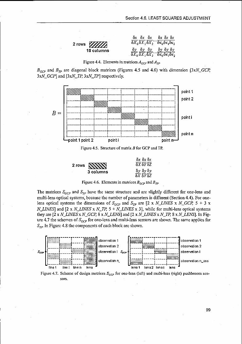
Section 4.6. LEAST SQUARES ADJUSTMENT
2 rows mm18 columns
Sx Sx Sx Sx Sx Sx
SX0SX i SX2' '
8k0SkiSk2
Sy 8y Sy Sy Sy Sy
SX0 SXX SX2 '"Sk08ki8k2
Figure 4.4. Elements in matrices ACCP and ATP
BGCP and BTP are diagonal block matrices (Figures 4.5 and 4.6) with dimension [3xN_GCP,
3xN_GCP] and [3x2V_77? 3xN_TP] respectively.
B
1—point 1 point 2 point i point n-
Figure 4.5. Structure of matrix B for GCP and TP.
point 1
point 2
point i
point n
2 rows H3 columns
Sx Sx Sx
sxsysz
Sy SySyS^fSTSZ
Figure 4.6. Elements in matrices Bççp and BTP.
The matrices SGCP and STP have the same structure and are slightly different for one-lens and
multi-lens optical systems, because the number ofparameters is different (Section 4.4). For one-
lens optical systems the dimensions of SGCP and STP are [2 x NJLINES x NjGCP, 5 + 3 x
N_LINES] and [2 x NJLINES x NJTP, 5 + NJLINES x 3], while for multi-lens optical systems
they are [2 x NJLINES x NJGCP, 8 x NJLENS] and [2 x NJLINES x NJTP, 8 x NJLENS]. In Fig¬ure 4.7 the schemes ofSGCP for one-lens and multi-lens sensors are shown. The same applies for
STP In Figure 4.8 the components of each block are shown.
wrjrp:
>:i
I"""
r~-"t.--.---.-*
| taaïiiliiiiii SIIS
line 1 line i linen lens
observation 1
observation 2
observation i
observation n
observation 1
observation 2
observation i
observation n oss
lensl lens2 lensi lens
Figure 4.7. Scheme of design matrices SCCP for one-lens (left) and multi-lens (right) pushbroom sen¬
sors.
99

Chapter 4. INDIRECT GEOREFERENCING
2 rows
3 columns
2 rows
5*c S*c S*
8AxP/c SAyP/c 60
8^ ^c 8y
8Axp/c bAyp/c 89
8x 8x 5x 8x 8x 8x
8/ Skx Sk2 8px Sp2 8s
Sy Sy_ 5y _8y_ 8y_ 8y_6 columns 8/ 8kx 5À:2 8pj 5p2 8sy
Figure 4.8. Elements in matrices SCCP and STP
4.6.3.2 External orientation constraints
The design matrices describing the constraints on the polynomials' continuity are called C„, with
n=0, 1,2, according to the degree ofthe derivatives. They are obtained from Equations 4.29,4.30and 4.31. The size of the matrices is [6 x (N_S-1), 18 xN_S].The structure of matrix C0 that describes the constraint on the continuity of the functions is
shown in Figures 4.9 and 4.10. The design matrix describing the first order constraint, called Cj,and the design matrix describing the second order constraint, called C2, are shown in Figures
4.11,4.12,4.13 and 4.14.
4.6.3.3 Initial values of PPM parameters
The unknown PPM parameters are fixed to the initial values by means of pseudo-observations.The design matrix describing the pseudo-observations for the PPM parameters is called F.
According to the formulas introduced in Section 4.5.2.2, the matrix F is a unit diagonal matrix,with dimension equal to the number ofPPM parameters [lSxNJS, lBxNJS],
4.6.3.4 Initial values of APs
The matrix that describes the pseudo-observations on the self-calibration parameters (AxP, AyP,
kj, k2, pj, p2, sy and 9) is a unit diagonal matrix, called S, with dimension [dimJS, dim_S]. As
shown in Section 4.4, the dimension dim_S is: NJLENS x 8 (multi-lens case) and 5+3 x NJLINES
(single-lens case).
4.6.3.5 Initial values of GCP coordinates
The ground coordinates of the GCPs are introduced in the model as pseudo-observations. The
observation matrix, indicated with letter E, is a diagonal matrix with dimension [3 x NJ3CP, 3 x
N_GCP].
4.6.3.6 Final matrix
The single blocks are positioned into the final design matrix (indicated with letter A), taking into
account the structure of the vector x, containing the unknown parameters of the model. In details,vector x contains:
•
xEO: PPM parameters (18 x N_S)•
xTP: TPs ground coordinates (3 x NJTP)•
xGCP: GCP ground coordinates (3 x NjGCP)•
xsc: self-calibration parameters (5+3 x NJLINES for single-lens optical systems and 8 x
NJLENS for multi-lens optical systems).
100

Section 4.6. LEAST SQUARES ADJUSTMENT
c0=
segment 1 segment 2 segment i
Figure 4.9.Structure of matrix C0.
T-_aï8BS»
segment N_B
— =111 —s.100
Figure 4.10.Single blocks in matrix C0.
segmenti segment 2 segmenti
Figure 4.11.Structure ofmatrix Cx.
segment N_B
_ =012 — =0-10
Figure 4.12.Single blocks in matrix Cx.
C,
segmenti segment 2 segmenti segment N_B
Figure 4.13. Structure of matrix C2.
_ =001 — =00-1
Figure 4.14.Single blocks in matrix C2.
Equations 4.64 and 4.65 and Figure 4.15 show the components ofvector x and design matrix A.
KEO
\.TP
XCCP
xsc
(4.64) A =
AGCP
Slj-p
Co
Cx
C,
B
Sgcp
TP STP
(4.65)
101

Chapter 4. INDIRECT GEOREFERENCING
The final observation system results
VGCP~
vTP=
VC0=
vCl =
VC2=
VF=
V£=
^GCPxEO + Sqcpxsc
^tpxeo + BTPxTp +SGCPxsc
Cqxeo
CxxEO
C2xE0
FxEO
Ex,
-lTP >P<
-lTP ;P
GCP
TP
-lco >PCO
CI
C2
GCP
-lex 'A
~^C2 A,
-IF 'Af
~h '^E
~'s >Ps
(4.66)
The matrices Pxx are the weight matrices of the single observations groups. They form the com¬
plete weight matrix Pu, a diagonal matrix with structure
Pn =
GCP
TP
CO
CI
C2
EO
(4.67)
Calling « the number of observations and u the number ofunknowns, the dimensions ofx, A and
Pn are [u, 1], [n, u] and [n,n] respectively.The resulting normal matrix N, obtained by Equation 4.46, has dimensions [u, u], is symmetricand sparse.
18xN_S
3xN_TP
3xN_GCP
dim_S
VE0
HP
HSCP
vsc
18xN_S 3xN_TP 3xN_GCP dim_S
2xN_LINES
xN_GCP
Agcp i r1 "GCP Sgcp
2xN_LINES
xN_TP
Ajp
Co
BTP"
j STP
6x(N_S-1)
6x(N_S-1) c,
6x(N_S-1) c2
18xN_S F
3xN_GCP
dim_S
1 E j*SSSSS«S$«f
w-„g——,
Figure 4.15.Structure of design matrix (right) and unknown vector (left).
102

Section 4.6. LEAST SQUARES ADJUSTMENT
4.6.4 Solution of linear system
Now the system
Nx = z (4.68)
must be solved with respect to x.
The normal matrix N is composed by blocks with different design: diagonal, hyperdiagonal, null
and sparse matrices. It is a complex structure with a variable number of submatrices, dependingon the parameters to be modelled. Such a structure needs to be treated with suitable algorithms,in order to reduce the storage and the computing efforts. The success of the methods depends on
the degree with which, in the reduction, the filling with non-zero elements can be limited, on the
extend to which the zero elements can be kept out of the numerical process and on the use of sim¬
ple and fast routines for the computation of the solution.
The main methods used for the solution of general least squares problems are based on LU fac¬
torization, Cholesky factorization and QR factorization. In all three methods a matrix is decom¬
posed into the product of two matrices with specific characteristics that render the calculation of
the solution more simple. In literature different publications can be found about the comparisonof the three methods (Choi et al, 1994, Dongarra, 1995, Hairer and Wanner, 1996).In our model the normal matrix is solved with the LU decomposition. According to this method,the normal matrix AT is written as the product oftwo matrices
N = LU (4.69)
where L is lower triangular (with elements a;/- only on the diagonal and below) and Uis upper tri¬
angular (with elements ß,y only on the diagonal and above). For the case of a [n,n] matrix, Equa¬tion 4.69 becomes
"11 "12 • "In
"12 "22 • "2n=
"41 "43 • «4«
au 0 0 o]a21 a22 0 0
0
cx„, an2 ... «J
ßll ßl2 - ßl„
0 ß22 - ß2„
0 0
o o 0 ß„n
(4.70)
Using this decomposition, the linear set
Nx = (LU)x = L(Ux) = z
is solved by first solving for the vectory such that
Ly = z
and then solving
Ux = y
(4.71)
(4.72)
(4.73)
The advantage of breaking up one linear set into two successive ones is that the solution of a tri¬
angular set of equations is quite trivial. Thus, Equation 4.72 can be solved by forward substitu¬
tion as follows
* =
Wi
yt = — +1
a,,-
i-i(4.74)
i = 2,3, ...,n
while Equation 4.73 can then be solved by back-substitution
103

Chapter 4. INDIRECT GEOREFERENCING
x =A
"
Vnn
yr 2 M;. y=l+l
(4.75)
i = n — 1,71-2, ...,1
For the stability of the method, pivoting is essential. Pivoting consists of the selection of a advan¬
tageous pivot element for the divisions required during the processing. The pivot element is cho¬
sen as the largest element on the diagonal. Only partial pivoting (interchange of rows) can be
implemented efficiently. However this is enough to make the method stable. This means, inci¬
dentally, that a row-wise permutation ofN, not actually N, is decomposed into LU form.
Equations 4.74 and 4.75 total (for each right-hand side z) n2 executions of an inner loop contain¬
ing one multiply and one add. If we have « right-hand sides which are the unit column vectors
(which is the case when we are inverting a matrix), then taking into account the leading zeros
reduces the total execution count of Equation 4.74 from 1/2 n3 to 1/6 n6, while Equation 4.75 is
unchanged at 1/2 n3. Once the LU decomposition in applied on N, all the desired right-hand sides
can be solved, one at a time (Press et al, 1992, pp. 43-44).
4.7 ANALYSIS OF RESULTS
When the bundle adjustment is completed, the internal and external accuracy of the ground coor¬
dinates of the observed points are analyzed. The correlations between the unknown parametersare studied in order to remove any over-parameterization. A blunder detection is also performed.These topics are described in details in the following paragraphs.
4.7.1 Internal accuracy
Sigma naught (indicated with ô0 ) is the a-posteriori standard deviation of unit weight. It is cal¬
culated using the vector v, computed with Equation 4.37, and the system redundancy (differencebetween number of equations and number ofunknown parameters)
(4.76)yn-u
Using the matrix Q^ defined as
ô0 =
\vTPv*\n-u
Qxx = N~l
Kxx = Oo Qxx
(4.77)
the covariance matrix K„ is calculated as
(4.78)
Ka is symmetric. The general diagonal element
àkt = àojq^t (4.79)
represents the mean-square errors of the individual unknown xk. The non-diagonal elements
occupying the position (ij) represent the covariances between the unknowns xt and xP
The planimetric and height precision of the ground coordinates of GCPs and TPs are calculated
separately as follows
104

Section 4.7. ANALYSIS OF RESULTS
2 tr(Kxx) 2 tr(Kyxx) , /*•(*„) (4.80)
gy
S S
where
o~x, rj^, and oz : standard deviation in X, Yand Z coordinates
Kxxx, Kxx and Kzxx: parts of^.corresponding toX, YandZ coordinates ofGCPs (or TPs)
g: number of points.
4.7.2 RMSE calculations
The TPs with known ground coordinates are used as Check Points (CPs). The estimated ground
coordinates [x Y Zj are compared to the correct ones [Xcort, Ycoir, Zcorr] and the RMSE are calcu¬
lated as
M CP N_CP AffP2
^(X-XC0J ^Y-Ycorr) )^(Z-Zcorr)RMSEX='-^ RMSE2 = '-^ RMSE2 = '-^ (4.81)
NJOP NJOP N_CP
where NJCP is the number of CPs.
4.7.3 Correlations
An investigation of the determinability of the additional parameters is also required in order to
avoid over-parameterization. For this task the correlations otJ between the parameters are calcu¬
lated as
Py = -tM= (4.82)daii
'
Ijj
where q^ are the elements of the matrix defined in Equation 4.77 in position (ij). Absolute values
of p,y close to 1 indicates high correlation between parameter x,. and Xj. If highly correlated
parameters are found, one of the two is manually fixed to constant values using pseudo-observa¬tions (Section 4.5.2 and Section 4.5.3).
4.7.4 Blunder detection
As the true errors vx and vy of the adjustment system (Equation 4.28) are not available, the imagecoordinates observations are tested for blunders using Griin's approach for photogrammetricblock adjustment proposed in (Grün, 1982). This approach is based on Baarda's data snoopingtechnique. According to the test, for each observation i the value wt
G(4.83)
is computed, with ôv = à0Jqvv, where Jqvv is the /-th element of the matrix QvV> defined as
ßvv = Pu'1 - A(ATPnA)XAT (4.84)
105

Chapter 4. INDIRECT GEOREFERENCING
If the null-hypothesis
Hv0i: E(vt) = 0 (4.85)
is true, wt is i-distributed. If the redundancy of the system is large enough, the % distribution can
be replaced by the Student distribution, which is far easier to handle.
The blunder detection is run at the end of the adjustment. The observations that are detected as
blunders are manually removed and the adjustment is repeated.
4.8 FORWARD INTERSECTION
Once the parameters modelling the internal and external orientation are estimated, it is possibleto calculate the ground coordinates of any point measured in the images. The algorithm for the
forward intersection is based on the principles described in Section 3.3. For each lensy', the pointcoordinates in the camera systems are projected into the ground system with
X Xc dxjY = Yc + R(a>c,<pc,Kc) dyjZ Zc_ w
kS((Oc, tpc, Kc> «y> ß;. 7;)
x - xPj + Axj
y-yPJ+Axj (4.86)
where
[X, Y, Z\: point coordinates in the ground system;
[Xc, Yc, Zc]: PC position in the ground system
[x, y] : point coordinates in the camera system
[xPj; yPJ] : principal point coordinates of lensy in the camera system
[Axy, Ayj\'. terms containing self-calibration parameters for lensy
/: focal lengthh scale factor
dxj, dyp dzj: relative position of each lensy* with respect to the central one
0Cy, ß-, jf. relative attitude of each lensy with respect to the central one
i?(C0c,(pc>Ko': rotation from camera system of the central lens to ground frame
? = R((oc, 9C, kc) • M(a.j, ßy, Yj): complete rotation from camera system ofthe off-nadir lensy
to ground system
M(ajt ßy, Y)'- rotation from camera system of the off-nadir lensy to camera system of the cen¬
tral lens.
Imposing the intersection of two homologous rays, the ground coordinates of the points mea¬
sured in two or more images can be estimated through a forward intersection.
In Equation 4.86 the external orientation parameters are calculated introducing the estimated EO
parameters in Equation 4.9 or Equation 4.12, if GPS and INS observations are used. In the same
way [Axy, Ayf\ are computed with Equation 4.26 (one-lens system) or Equation 4.27 (multi-lens
systems). The solution is estimated in two steps, using the algorithm described in Section 3.3.
This algorithm is used not only for the calculation of the ground coordinates of the check points,but also for the generation ofDSM and DTM. In fact if a large number of points are matched in
the images, using the forward intersection a 3D point cloud is automatically created in the ground
system. By mean of suitable interpolation algorithms, a regular surface (DSM) is created.
106

Section 4.9. SUMMARY AND COMMENTS
4.9 SUMMARY AND COMMENTS
In this Chapter the mathematical formulation of the indirect model for the georeferencing of
CCD linear array sensors has been described.
The model is based on the collinearity equations, which are extended in order to include the sen¬
sor internal and external orientation modelling. The internal orientation is improved by takinginto account the lens distortions and the displacements and rotations of the CCD lines in the focal
plane. The external orientation is modelled with second order piecewise polynomials (PPM)depending on time or image-line number. According to this approach, the trajectory is divided
into a suitable number of segments and for each segment it is modelled with parabolic functions.
Additionally, the GPS and INS measurements, which are indispensable for pushbroom sensors
earned on airplane or helicopter, can be integrated in the adjustment and corrected from system¬atic enors (shifts and misalignments, first and second order errors). The number of segments is
decided in each case study according to the trajectory length and smoothness. In general, for sat¬
ellite orbits, 2 segments are sufficient, but for sensors carried on airplane or helicopter a largernumber of segments is recommended, as the trajectory is less smooth. The system is solved with
a least-squares adjustment, using a suitable number of ground control points. The weights for the
observations (collinearity, pseudo-observations for the unknowns) are calculated according to the
accuracy of the corresponding measurements.
As mentioned in the Introduction, nowadays many models with different complexity and rigorexist. Few ofthem include the self-calibration, which is recommended ifthe instrument's labora¬
tory calibration is not available. Concerning the sensor position and attitude modelling, Lagrangepolynomials or second order polynomials are often used; in some cases linear functions are pre¬
ferred for satellite trajectories. This option is also included in our model, because the second
order parameters in the PPM can be fixed to zero using highly weighted pseudo-observations.Taking into account the rigorous models presented in literature, few of them can be used for any
pushbroom sensor carried on satellite and even fewer can be used for airborne sensors too. Our
model, on the other hand, has been designed in order to be as flexible as possible for the georef¬erencing of a wide class of pushbroom sensors. In fact it uses a quite flexible function for the
external orientation modelling and takes into account systematic errors due to lens distortions
and CCD lines displacements that may occur during the image acquisition. In the design phase,the main idea was to create a model that could describe the image acquisition ofpushbroom sen¬
sors with different characteristics, and then, according to the specific case study, to estimate onlythe parameters of interest. For example, the number of segments is decided according to the plat¬form (satellite, airplane or helicopter), the length of the trajectory and the distribution of groundcontrol and tie points (at least one tie point in each segment). The estimation of only the parame¬
ters of interest is possible thanks to the use of pseudo-observations. In fact any parameter can be
fixed to constant values using highly weighted pseudo-observations. This option may overcome
the risk of over-parameterization. In order to select the parameters of interest, the analysis of the
significance of each parameters and the correlation with the other unknowns are fundamental. In
our software this selection is made manually.Due to the fact that for each case study the number ofparameters is different, the minimum num¬
ber of ground control points required in the bundle adjustment is not unique. In general the num¬
ber ofunknowns depends on the number of segments in the PPM, the degree of the functions and
which self-calibration parameters are estimated (Figure 4.15). Considering a simple case with
two-line sensor carried on satellite, the trajectory modelled with two second order polynomialsand no tie points, the number of unknowns is 36. As the constraints for the PPM continuity give18 equations and each GCP give 4 observation equations, at least five GCPs are required for the
solution of the system. In order to increase the redundancy, a minimum of six GCPs are recom-
107

Chapter 4. INDIRECT GEOREFERENCING
mended. Of course the distribution of the GCPs may influence the number of GCPs required.Concerning the flexibility ofthe model, new cameras can be easily integrated. In fact the requiredsensor information (number of linear arrays, number of lenses, focal length, number of detector
elements in each line, viewing angles) are accessible in literature as well as in the web. If no
information on the sensor internal orientation is available, the model supposes that the CCD lines
are parallel to each other in the focal plane and perpendicular to the flight direction and estimates
the systematic errors through the self-calibration. Concerning the external orientation, in case of
spaceborne sensors the satellite's position and velocity vectors, usually contained in the ephem¬eris, are required in order to compute the initial approximations for the PPM parameters. If this
information is not available, the Keplerian elements can be used to estimate the nominal trajec¬tory. For pushbroom scanners carried on airplane or helicopter the GPS and INS measurements
are indispensable, due to the unpredictability of the trajectory.
108

Section 4.9. SUMMARY AND COMMENTS
109

Chapter 4. INDIRECT GEOREFERENCING
110

5
PREPROCESSING
Before applying the algorithms for the georeferencing of the images, some operations are
required in order to prepare the input data. The pre-processing includes both the analysis of the
metadata files for the extraction of the required information and the radiometric improvement of
the images in order to facilitate the points measurement, which is usually performed with least-
squares template matching.
5.1 METADATA FILES FORMATS
In order to extract the information regarding the sensor geometry, the image characteristics and
the initial approximations of the external orientation, the metadata files must be analyzed. Due to
the variety of formats, only the metadata files of the data used in this work will be taken into
account. The information required for the image georeferencing with the developed sensor
model are summarized in Table 5.1. Usually one metadata file is associated to each satellite
scene. In case ofMISR the same file contains the scenes and the image characteristics only. Theinformation on the camera geometry are contained in the Camera Geometric Model (CGM) file,downloadable from NASA, while the ephemeris must be requested at the JPL NASA center in
Pasadena, California, USA.
The metadata files are quite different from one satellite to the other. Apart of the file format (text,HDF -Hierarchical Data Formatfile-, XML -Extensible Markup Language-, ...), the kind of data
contained and the reference systems used are not standard.
For ASTER the sensor position and velocity and the acquisition time are given for a defined
number of so-called lattice points (Figure 5.1), whose number varies with the channels. In
Table 5.2 the number of lattice points in the across and along track directions for each channel is
given. The lattice grid covers an area which is larger than the scene in the along-track direction.
The position of the scene area in the lattice grid in the along-track direction (segment called ojf-
111

Chapter 5. PREPROCESSING
set in Figure 5.1) varies in each scene.
The pointing vectors in SPOT-5/HRS metadata files are described by the two angles \|/y and \|/x,
defined in the orbit system, as shown in Figure 5.2.
Table 5.1. Main characteristics ofmetadata files used in this work. Abbreviations: RS = reference system;
pos= position; vel = velocity; att = attitude.
Data EROS-A1 SPOT-5/HRS ASTER MOMS-P2 MISR
number of files 1 1 1 1 more
format text (76 lines) DIMAP HDF TEXT HDF
acquisitiontime format
UTC UTC UTC UTC UTC
acquisitiontime density
first and last
linescenter line lattice points
first and last
lines every line
integrationtime yes yes yes no no
state vector
formattime, position,velocity
time, position,velocity
time, position,velocity
time, position,velocity
time, position,velocity
state vector
RSECl ECR ECR ECR ECl
state vector
density every 10 lines
every 30s
(pos, vel),every second
(att)
lattice pointsevery second
(pos), everyline (att)
every 1.024s
focal length no no yes yes yes
pixel size no no no no yes
calibration noyes, pointingvectors
no yes yes
viewing angles yes (initial andfinal) yes yes no yes
0
Across-track Lattice Points
2 n-1 n
offsett
1
**?tS* "S*!*ïîï^| «$£! •*-.-* «WNN \ ts-fc, **J£ S-
Along-track 2Lattice Points
m-1
m
^«*- «i i
-, ^ , „ *u._.
Defined Scene Area
Figure 5.1. Lattice points structure in ASTER scenes.
m and n are lattice points counters.
Table 5.2. Number of lattice points for
ASTER.
BAND n across m along
VNIR
1,2,3N
10 11
VNIR3B 10 14
SWIR 103 105
TIR 10 10
112

Section 5.2. INFORMATION EXTRACTION FROM METADATA FILES
5.2 INFORMATION EXTRACTION FROM METADATA FILES
The metadata files are indispensable to extract the information on:
• external orientation
• camera geometry• acquisition time
• internal orientation
External orientation. For the dataset used in this work, two approaches have been used to cal¬
culate the sensor external orientation. In case of MOMS-P2, DLR provided the sensor positionmeasured with GPS and the sensor attitude measured with INS. The data have been interpolatedfor each line using cubic splines (Section 3.2.3) and used to compute the initial approximation of
the external orientation parameters, according to Equations 4.62 and 4.63.
In the other cases, the state vectors containing the platform position and velocity at some instants
of time have been used to calculate the sensor attitude as described in Section 3.2.2. Again, the
values have been interpolated for all the image lines.
As an example, the calculation of the external orientation in case of the MISR test is described.
For simplicity, 10 state vectors of the original 256 are reported.From the ephemeris for EOS-AMI where MISR is mounted, the position is extracted in ECl sys¬
tem (Section B.4)272025550.435975015
272025551.459975004
272025552.483975053
272025553.507975042
272025554.531975031
272025555.555975020
272025556.579975009
272025557.603974998
272025558.627975047
272025559.651975036
-2803974.875
-2807005.250
-2810032.500
-2813056.375
-2816076.875
-2819094.125
-2822108.125
-2825118.750
-2828126.000
-2831130.000
2758826.875
2764557.625
2770285.000
2776009.125
2781730.125
2787447.750
2793162.000
2798873.125
2804580.875
2810285.375
5879809.000
5875679.250
5871542.625
5867399.125
5863248.625
5859091.250
5854927.000
5850755.750
5846577.625
5842392.625
The format is time in seconds, X, Y, Z in meters. After the conversion to ECR system (SectionB.5), the position (X, Y, Z) is
3850830.658387
3857340.029129
3863844.738769
3870344.752453
3876840.173866
3883330.863947
3889816.822402
3896298.187611
3902774.751231
3909246.686285
805468.538465
804526.237219
803582.237730
802636.263701
801688.246829
800738.430798
799786.816653
798833.162750
797877.608784
796920.190498
5879445.414008
5875315.261130
5871178.233657
5867034.331620
5862883.430020
5858725.653841
5854561.003084
5850389.352762
5846210.827878
5842025.428415
During this transformation a rotation around Z-axis has been applied. The effect ofthe rotation is
evident if the geographic coordinates (latitude and longitude in degrees, height in meters) are
considered, In fact the longitude changes during the transformation, while the latitude and heightremain stable:
position in ECl system56.377077 135.465010 710944.027149
56.317018 135.436511 710931.008990
56.256951 135.408105 710918.052712
56.196878 135.379786 710905.108090
56.136798 135.351553 710892.120211
56.076710 135.323410 710879.144796
position in ECR system56.371794 11.814085 710942.203262
56.311737 11.781295 710929.184354
56.251673 11.748597 710916.227333
56.191602 11.715987 710903.281974
56.131524 11.683463 710890.293368
56.071439 11.651029 710877.317231
113

Chapter 5. PREPROCESSING
56.016616 135.295356 710866.181697
55.956514 135.267387 710853.176009
55.896405 135.239504 710840.133110
55.836289 135.211708 710827.152052
56.011347 11.618684 710864.353418
55.951247 11.586424 710851.347022
55.891141 11.554250 710838.303423
55.831027 11.522163 710825.321673
The attitude is calculated using the position and velocity vectors in ECR systems, according to
Equations 3.16, 3.17 and 3.18, and results in
-0.136150
-0.136087
-0.136024
-0.135960
-0.135897
-0.135833
-0.135769
-0.135704
-0.135640
-0.135575
.575604
.576701
.577797
.578894
,579990
.581087
.582184
-0.583280
-0.584377
-0.585473
The same attitude in ECl system is
-0.438708 -0.407550
-0.439777 -0.408016
-0.440847 -0.408482
-0.441917 -0.408947
-0.442987 -0.409412
-0.444058 -0.409877
-0.445129 -0.410341
-0.446201 -0.410805
-0.447273 -0.411268
-0.448346 -0.411731
The external orientation values in ECl system are:
X1=2803974.875
CO^-0.44
and in ECR system they are:
Xr=3850830.658
CO =-0.14
Yr=2758827.875
<pr=-0.41
Yr=805468.538
«V=-0.57
-0.047969
-0.048126
-0.048283
-0.048441
-0.048599
-0.048756
-0.048914
-0.049072
-0.049230
-0.049389
-1.127126
-1.127550
-1.127974
-1.128399
-1.128824
-1.129250
-1.129677
-1.130105
-1.130533
-1.130961
Zr=5879809.000
K= -1.13
Zr=5879445.414K= 0.05
Camera data. For the direct and indirect georeferencing models, the information about the
instruments required are: number of lenses, number of linear arrays for each lens, number of
detectors in each line, viewing angle and focal length ofeach lens. Usually these information are
available in the metadata files. Otherwise they are found in literature or in the web sites of the
corresponding space agencies or data distributors. For example, in case of SPOT-5/HRS the
(nominal) focal length of the sensor (580mm) was found in (Gleyzes et al, 2003), while the
viewing angle of each lens and the pixel size were calculated from the looking vectors (Figure5.2), which have component (\|fx, \j/v 1). Calling xj/x(i) and \|/Y(0 the values of \|/x and yY for the
pixel in position /, the off-nadir viewing angle of each lens (angle ß) was calculated as the aver¬
age of the along-track component of the looking vectors:
ß =
yx( 12000) -Vjf(l)12000
while the pixel size in across-track (p) directions was calculated as
Py = fx?y( 12000) -vj/,,(l)
12000
(5.1)
(5.2)
114

Section 5.2. INFORMATION EXTRACTION FROM METADATA FILES
Figure 5.2. Looking vectors for SPOT-5/HRS (SPOT Satellite Geometry Handbook 2002, p.29).
Acquisition time. Usually the acquisition time of the first line t0 and the integration time Atsare provided, therefore Equation 3.19 in Section 3.2.3 can be applied. This is the case of EROS-
Al and MOMS-P2. For MISR the exact acquisition time of each image line is already available
in the metadata file and for SPOT-5/HRS the acquisition time of the central line (line 6001) is
given together with the integration time Ats, therefore the acquisition time of any other line can
be estimated with Equation 3.19 using the center line as reference.
In case ofASTER the acquisition time of each image line is interpolated from the values in cor¬
respondence of the lattice points. Taking into account the VNIR 3N and 3B images used in this
work and later described in Section 6.4, the lattice grid covers an area of 4100x4800 pixels
(image 3N) and 5000x5600 pixels (image 3B). The lattice point «=0 is located at line 263 and
204 for 3N and 3B respectively (offsets of 263 and 204 lines). The acquisition time of imagelines 1 and 4200 (image 3N) and image lines 1 and 5400 (image 3B) are linearly interpolated as
,.
,
'-263 + 4800~ '-263,0/:,
, n
'»= '"*" + 48ÔÔ (263 + 1}
(5.3)t- 263 + 4800
~'-263,
for image 3N and
'4200 = '-2634300
-""(263 + 4200)
'-204 + 5600 *-204f2fH , x
h ~ '-204 + 56ÖÖ (204 +1'(5.4)
'5400 = '-204 + ,Zn "(204 + 5400)t- 204 + 5600 ~'-204,
4800
for image 3B.
Additional parameters. These parameters include the sensor laboratory calibration. In case of
MOMS-P2, a report contains the results obtained in the laboratory calibration as described in
Section 2.4.3. In case ofMISR, the parameters estimated in the on-flight calibration are reportedin an extra file, called CGM (Camera Geometric Model). The procedure is explained in
Jovanovic et al, 1999b. In case of SPOT-5/HRS the camera calibration consists of the pointingvectors ofeach pixel in the linear array (Figure 5.2).
115

Chapter 5. PREPROCESSING
5.3 RADIOMETRIC PREPROCESSING
In our processing chain 8-bit greyscale images are used. They are generated either from a singlecolor channel (for example red channel in case of MISR, near infrared channel for ASTER) or
from the panchromatic channels (as in case of EROS-Al, SPOT-5/HRS, MOMS-02). All the
original images used in this work have the radiometric resolution of 8-bit (usually 8-bit and 11-
bit images are supplied by the providers). If necessary, images with different radiometric resolu¬
tions may be reduced to 8-bit with a linear stretching between the minimum and maximum val¬
ues.
The radiometric characteristics of the images are closely dependent on the acquisition aspects,like the sensor view angle, the sun angle and shadowing, the seasons, the atmospheric conditions
and whether the scene is recorded in mono or stereo (Baltsavias et al. 2001). As there is limited
opportunity for the user to dictate specific imaging dates, times and weather conditions, the radi¬
ometric quality may be improved by analyzing the initial histogram and applying algorithms for
gamma correction, contrast enhancement, histogram equalization or a combination ofthem (Wal¬lis filter). The resulting histograms, obtained with Adobe Photoshop (Adobe Photoshop, 2004)are shown in Figure 5.4.
5.3.1 Standard algorithmsGamma correction. This is a nonlinear transformation that changes the brightness ofan imagein order to compensate for nonlinear responses in imaging sensors. The general form for gamma
correction is
i
imgnew(x,y) = img(x, v)Y (5.5)
Ify= 1.0, the correction is null. If 0 < y< 1.0, the conection creates exponential curves that dark¬
ens an image. Ify>1.0 the result is a logarithmic curve that brightens an image.
Contrast enhancement. The contrast enhancement increases the total contrast ofan image by
making the high grey values higher and the low grey values lower at the same time. It does this
by setting all the components below a specified lower bound to zero, and all components above a
specified upper bound to the maximum intensity (that is, 255). The radiometric values between
the upper and lower bounds are set to a linear ramp ofvalues between 0 and 255.
Histogram equalization. It is similar to the contrast enhancement, but the same number of
pixels is approximately assigned to each output grey value. It is one of the most important part of
the software for any image processing. The goal of histogram equalization is to obtain a uniform
histogram, by redistributing the intensity distributions. If the histogram of any image has many
peaks and valleys, it will still have peaks and valley after equalization, but peaks and valley will
be shifted.
Wallis filter. The Wallis filter combines the radiometric equalization and the contrast enhance¬
ment in an optimal way (Wallis, 1976, Baltsavias, 1991, Valadan Zoej and Foomani, 1999). It is
an adaptive, local filter, which has been extensively used at our Institute in image preprocessingfor matching of satellite (e.g. Baltsavias and Stallmann, 1993, Baltsavias et al 2001), airborne
(Baltsavias et al, 1996a) and close range images (Grün et al, 2003a).The filter is defined with the objective of forcing the mean and standard deviation of an image to
given target values. The filtered image (imgnew) is calculated from the original image (img) as
imgnew(x, y) = img(x, v) • r, + r0 (5.6)
116

Section 5.3. RADIOMETRIC PREPROCESSING
where
r = cSf
1
csg + (\-c)-sf (5/7)
r0 = bmf + (l-b-rl)-mg
(mg,sg) are the original mean and standard deviation ofeach block, (my sj) are the target mean and
standard deviation for every block, b (0<b<l) is the brightness forcing constant and c
(0 < c < 1 ) is the contrast expansion constant.
The filter works as follows. First the image is divided into rectangular blocks of given size and
defined distance between the block centers. Then the parameters r0 and rt are computed in each
block. Finally each pixel of the original image is transformed with r'0 and r\, which were bilin-
early interpolated from the r0 and r7 values of the 4 neighboring block centers. In areas with the
same grey values (e.g. saturated areas) the filter cannot create any texture, but in areas with weak
texture patterns the filtering strongly enhances the texture so that the images are optimized for
matching (Seiz, 2003). As example, the contrast enhancing effect of the Wallis filter on MOMS-
P2 scenes is shown in Figure 5.3.
Figure 5.3. Zoom in MOMS-P2 channel 7 before (a) and after (b) the radiometric equalization and
contrast enhancement by Wallis filter. For more details about the scenes, see Section 6 2.
5.3.2 Ad-hoc filters
In some cases special blurring effects require the implementation of specific filters to remove
them. In the following, two examples of special filters applied on images used in this work are
shown. In ASTER level 1A scenes, which are not radiometrically corrected, it is evident the pres¬
ence of vertical stripes. For their conection the coefficients contained in the HDF files are used.
These radiometric coefficients are generated in two steps. The first step is the off-line generationof radiometric coefficients at predefined reference temperature. These coefficients are effective
for a long time, depending on the instrument stability, and available in radiometric correction
data base files along with the temperature coefficients. Destriping parameters are generated from
the image data analyzing the image data obtained during the initial checkout operation period.The second step is an on-line process executed during level 1 product generation to correct the
radiometric coefficients for instrument conditions such as the detector temperature, which may
117

Chapter 5. PREPROCESSING
Mean 88 26 Level
J StdDev 24 54 Count
Median 87 Percentile
Pixels 144000000 Cache Level 1
I Mean 12498
StdDev 19 23
1 Median 126
f Pixels 360000
fe>**ta*N, « "US,
(a)
Level
Count
Percentile
Cache Level 2
(b)
Mean. 127.76 Level
StdDev. 73 74 Count
Median 126 Percentile
Pixels 144000000 Cache Level 1
Mean 124 88
StdDev 49 69
Median 117
Pixels 144000000
Level
Count
Percentile
Cache Level 1
(c) (d)
Figure 5.4. Companson of 8-bit histograms in the original SPOT-5/HRS level 1 image (a), after gamma
correction (y=1.5) (b), after histogram equalization (c) and after Wallis filter (d).
change for every observation. Considering an image line, the radiometric value of each pixel is
corrected with the following transformation (Abrams et al, 2002)
I = a- + dg
(5.8)
where v and / are the input and output values, a is a linear coefficient, g is the gain and d an off¬
set. These parameters are constant for all image lines. Figure 5.5 shows the positive effect of this
filter, before and after applying the radiometric enhancement.
The second filter has been applied on MOMS-02 scenes in order to reduce the saturation in
regions covered by clouds. In this case a template containing the standard saturation striping hasbeen used to detect the saturated areas in the images through cross-correlation. Then a median
filter was applied. The result in a zoomed region is shown in Figure 5.6.
118
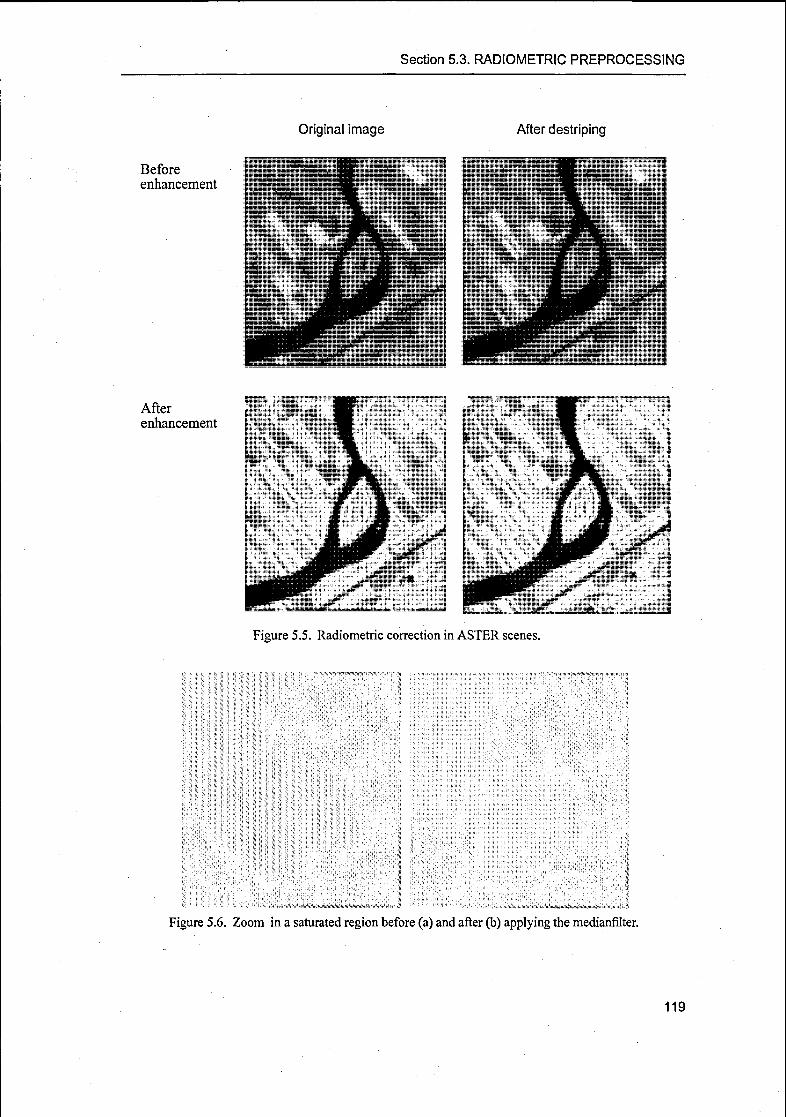
Section 5.3. RADIOMETRIC PREPROCESSING
Original image After destriping
Before
enhancement
After
enhancement
Figure 5.5. Radiometric correction in ASTER scenes.
wriM
^i^f^^Ä^i}ik*$öi!siidä&ä$$»!&^^ é
Figure 5.6. Zoom in a saturated region before (a) and after (b) applying the medianfilter.
119

Chapter 5. PREPROCESSING
120

6
APPLICATIONS
The sensor model presented in the previous Chapters has been used to orient images acquired by
pushbroom sensors with different geometric characteristics. In order to demonstrate the flexibil¬
ity of the model, images acquired with single- and multi- lens optical systems, synchronous and
asynchronous acquisition modes and different resolutions have been used, as reported in Table
6.1. Among the pushbroom sensors used for photogrammetric applications (Chapter 2), the
choice of the sensors to use for our tests depended exclusively on their availability. The MOMS-
02 dataset was available at our Institute, the MISR and ASTER ones was downloaded for free
(MISR) and at very low price (ASTER, 55$ per scene) by NASA, while the EROS-Al and
SPOT-5/HRS images came from external scientific collaborations.
In this Chapter the workflow followed in the data processing is summarized in Section 6.1, then
the results obtained with each dataset are described in the following Sections. For each dataset
the instruments and the data are described and the results obtained by the image orientation are
reported and commented. The results obtained using airborne sensors (SI-100) are described in
Poli, 2002b. Before the application with real data, the model was also tested on simulated data.
Part of these tests have been published in Poli, 2002a.
Table 6.1. Main characteristics of sensors analyzed in this Chapter.OPTICAL SYSTEM SYNCHRONOUS RESOLUTION SENSOR
one multi yes no high mean low
EROS-A1
SPOT-5/HRS
ASTER/VNIR
iMOMS-P2
MISR
121

Chapter 6. APPLICATIONS
6.1 WORKFLOW
For each sensor the analysis and processing of the data has been carried out following these
steps:1. Analysis of metadata files for the extraction of the acquisition time of each image line, the
sensor external and internal orientation (if available) and any additional information on the
images. These operations have been described in Section 5.2.
2. Radiometric preprocessing of the images in order to improve the radiometric quality and
facilitate the point measurement. This operation has been described in Section 5.3.
3. Measurement of object points. The image coordinates are usually estimated with templateleast-squares matching, while the ground coordinates are given by external providers (i.e.SPOT-5/HRS and EROS-Al cases) or are measured in topographic maps (i.e. MOMS-P2,ASTER and MISR cases), or in rectified scenes from other sensors (i.e. Landsat).
4. Preparation of input files for direct georeferencing. The required files are: sensor characteris¬
tics (number of lenses, number of viewing directions, number of CCD lines, viewing angles,
pixel size, focal length), image coordinates of tie points (row, columns) and external orienta¬
tion (position and attitude at certain time intervals). If the external orientation is not providedfor each image line but for a generic time interval (for example, the ephemeris observation
time), then for each image the file containing the acquisition time of each image line is
required. Thanks to this information, the external orientation for any line of interest is interpo¬lated with cubic splines for the corresponding acquisition time. The reference systems for the
external orientation accepted by the software are: the geocentric cartesian fixed system (ECR,Section B.5), the geographic system (Section B.6) and any local tangent systems (SectionB.7). An additional facultative file is the calibration file for each sensor (position of each
detector in the focal plane in the scanline system -Section B.2). More details about the format
of the input files are in Appendix C.
5. Direct georeferencing of the images. The ground coordinates of the tie points measured in the
images are estimated through a forward intersection using the available external and internal
orientation, as described in Chapter 3. The process accuracy is analyzed through the residuals
(RMSE) between the estimated and the correct ground coordinates of the points. In all the
case studies reported in this Chapter a sub-pixel accuracy in the RMSE could not be achieved
and the indirect georeferencing approach was used.
6. Preparation of input files for indirect georeferencing. The same input files used for the direct
georeferencing are needed. In addition the file containing the ground coordinates of the con¬
trol points is required. The reference systems accepted by the software are: the geocentric car¬
tesian fixed system (ECR, Section B.5), the geographic system (Section B.6) and any local
tangent systems (Section B.7).7. Indirect georeferencing of the images. A bundle adjustment is performed in order to estimate
the ground coordinates of the tie points, the piecewise polynomial model (PPM) parametersfor the external orientation and the self-calibration parameters, as explained in Chapter 4. The
program requires the number of ground control points (GCPs) and check points (CPs), the
accuracy of the image and ground measurements, the number of segments for the PPM func¬
tions, the PPM degree for each function and for each segment, the accuracy of the available
external orientation measurements, the self-calibration parameters to be estimated and the
maximum number of iterations. Different tests are performed varying the number and distri¬
bution of GCPs, the PPM parameters (number of segments, degree) and the number of self-
calibration parameters. In some cases the tests are limited by the small number of GCPs. The
adjustment is evaluated through both the internal accuracy (standard deviation of unit weighta posteriori, standard deviation of estimated parameters) and the external accuracy (RMSE of
122
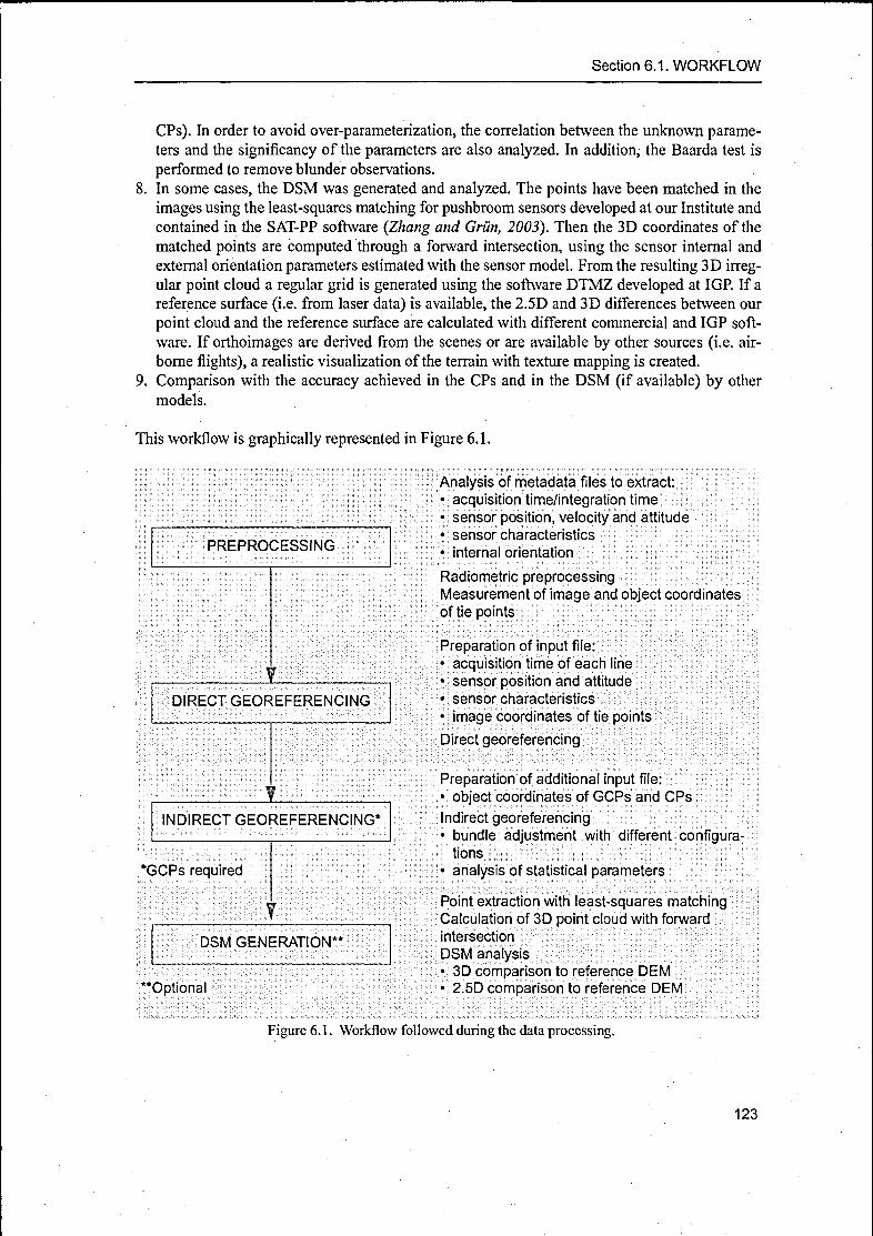
Section 6.1. WORKFLOW
CPs). In order to avoid over-parameterization, the correlation between the unknown parame¬
ters and the significancy of the parameters are also analyzed. In addition, the Baarda test is
performed to remove blunder observations.
8. In some cases, the DSM was generated and analyzed. The points have been matched in the
images using the least-squares matching for pushbroom sensors developed at our Institute and
contained in the SAT-PP software (Zhang and Grün, 2003). Then the 3D coordinates of the
matched points are computed through a forward intersection, using the sensor internal and
external orientation parameters estimated with the sensor model. From the resulting 3D irreg¬ular point cloud a regular grid is generated using the software DTMZ developed at IGP. If a
reference surface (i.e. from laser data) is available, the 2.5D and 3D differences between our
point cloud and the reference surface are calculated with different commercial and IGP soft¬
ware. If orthoimages are derived from the scenes or are available by other sources (i.e. air¬
borne flights), a realistic visualization of the terrain with texture mapping is created.
9. Comparison with the accuracy achieved in the CPs and in the DSM (if available) by other
models.
This workflow is graphically represented in Figure 6.1.
PREPROCESSING
DIRECT GEOREFERENCING
INDIRECT GEOREFERENCING*
*GCPs required
w
DSM GENERATION*
"Optional
Analysis of metadata files to extract:
• acquisition time/integration time
• sensor position, velocity and attitude
• sensor characteristics
• internal orientation
Radiometric preprocessingMeasurement of image and object coordinates
of tie points
Preparation of input file:• acquisition time of each line
• sensor position and attitude
• sensor characteristics
• image coordinates of tie points
Direct georeferencing
Preparation of additional input file:
• object coordinates of GCPs and CPs
Indirect georeferencing• bundle adjustment with different configura¬
tions
• analysis of statistical parameters
Point extraction with least-squares matchingCalculation of 3D point cloud with forward
intersection
DSM analysis• 3D comparison to reference DEM
• 2.5D comparison to reference DEM
Figure 6.1. Workflow followed during the data processing.
123

Chapter 6. APPLICATIONS
6.2 MOMS-02
The indirect georeferencing model was used to orient a stereopair acquired by the German
MOMS-02, mounted on the Russian MIR station during Priroda mission. The data were provided
by DLR.
6.2.1 Sensor descriptionThe Modular Optoelectronic Multispectral Stereo-scanner (MOMS-02) was developed by DLR
during the 80's. MOMS-02 is the first representative of a new along-track sensor generation,
designed for the combined stereo-photogrammetric and thematic mapping of the Earth's surface.
The history of MOMS starts from the early 70's, when the company Messerschmitt-Bölkow-
Blohm (MBB), now Daimler Benz Aerospace (DASA), carried flight experiments with the Elec¬
tro-Optical Scanner (EOS), built on the principle of the photo semiconductor sensors. Then the
first two-channel space sensor MOMS-01 was developed by MBB and flown successfully on two
Space Shuttle missions on the German "Shuttle Pallet Satellite" (SPAS, also developed by MBB)in 1983 and 1984. The further MOMS development was initiated and started under the supervi¬sion of the German Space Agency (DARA). MOMS-02 was first flown during the Second Ger¬
man Spacelab Mission D2 on Space Shuttle flight STS-55 and acquired data between the 26th
April and the 6th May 1993 (Seige, 1995). From April 1996 till March 2003, the MOMS-02
instrument was operational on the Priroda module of the Russian Space Station MIR, with the
name MOMS-2P (Seige et al, 1998). The station was flying along an orbit at a nominal height of
400km, with an inclination of 55° (Figure 6.2).
Figure 6.2. MIR orbit and coverage during D2 and Priroda missions (Source MOMS-02, 2004).
The major improvements of MOMS-2P compared with MOMS-02/D2 were: the long term
observation capability (more than one year), the coverage of higher latitude (between 51.6°), a
new high precision NAV (GPS and gyro) and a system multi-sensor approach in combination
with other Priroda sensors.
The MOMS-2P optical system consisted of five lenses, three ofwhich designated for the stereo¬
scopic panchromatic images and the other two for the multispectral images (Figure 6.3 and Fig¬ure 6.4). The central lens (channel 5), with a focal length of 660mm, formed the core of the
camera system. It allowed the high resolution imagery with a ground pixel size of 6x6m2 (flightaltitude 400km). In order to obtain a wide enough swath width in combination with this resolu¬
tion, two linear sensors were optically combined in the focal plane. In connection with the use of
124

Section 6.2. MOMS-02
the high resolution lens, there were two additional lenses, each with a focal length of237.2mm, a
ground resolution of 18m and an offnadir angle of +21.4° (channel 7) and -21.4° (channel 6)
respectively. In this configuration three-fold stereoscopic imagery was achieved (Figure 6.5). The
focal length of these lenses was chosen in a way to achieve an integral relationship between the
ground pixel sizes seen by the high resolution sense and the two inclined lenses by a ratio of 1: 3.
Two additional lenses, each with a focal length of 220 mm, enabled the multispectral imagingwith a total offour channels (channels 1, 2, 3,4). In order to simplify the image data analysis, the
ratio of the ground pixel size of the high resolution channel with that of these multispectral chan¬
nels was also selected to be 1:3. The detectors' size is 10u.m x 10p.m.
Figure 6.3. MOMS-02 sensor on its orbit Figure 6.4. MOMS-02 lenses (Source MOMS-02,
(Source MOMS-02, 2004). 2004).
Figure 6.5. MOMS-P2 acquisition geometry (Source MOMS-02, 2004).
The swath width for the high resolution channel is about 50km, depending on the recordingmode, and for the other channels, up to 105km. These values are relative to a nominal orbit alti¬
tude of 400km. The three viewing angles allow to image a strip on the Earth's surface, at three
different times and with the three different viewing angles (Figure 6.5). The fact that the three
images are recorded within only about 40 seconds makes it easy to correlate them, because of
their radiometric similarity.
125
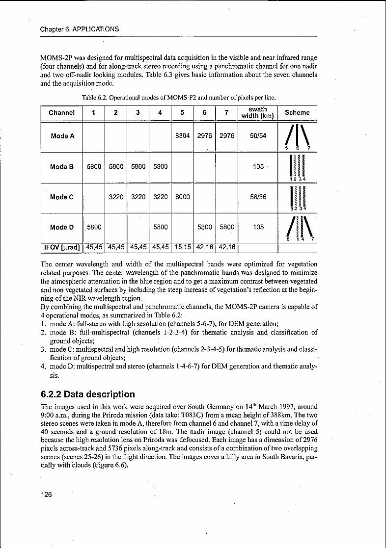
Chapter 6. APPLICATIONS
MOMS-2P was designed for multispectral data acquisition in the visible and near infrared range
(four channels) and for along-track stereo recording using a panchromatic channel for one nadir
and two off-nadir looking modules. Table 6.3 gives basic information about the seven channels
and the acquisition mode.
Table 6.2. Operational modes ofMOMS-P2 and number ofpixels per line.
Channel 1 2 3 4 5 6 7swath
width (km)Scheme
Mode A 8304 2976 2976 50/54 /l\5 6 7
Mode B 5800 5800 5800 5800 105 III12 34
ModeC 3220 3220 3220 6000 58/36111!I52 34
Mode D 5800 5800 5800 5800 105 /|l\6 14 7
IFOV [urad] 45,45 45,45 45,45 45,45 15,15 42,16 42,16
The center wavelength and width of the multispectral bands were optimized for vegetationrelated purposes. The center wavelength of the panchromatic bands was designed to minimize
the atmospheric attenuation in the blue region and to get a maximum contrast between vegetatedand non vegetated surfaces by including the steep increase of vegetation's reflection at the begin¬
ning of the NIR wavelength region.
By combining the multispectral and panchromatic channels, the MOMS-2P camera is capable of
4 operational modes, as summarized in Table 6.2:
1. mode A: full-stereo with high sesolution (channels 5-6-7), for DEM generation;2. mode B: full-multispectral (channels 1-2-3-4) for thematic analysis and classification of
ground objects;3. mode C: multispectral and high resolution (channels 2-3-4-5) for thematic analysis and classi¬
fication ofground objects;4. mode D: multispectral and stereo (channels 1-4-6-7) for DEM generation and thematic analy¬
sis.
6.2.2 Data description
The images used in this work were acquired over South Germany on 14th March 1997, around
9:00 a.m., during the Priroda mission (data take: T083C) from a mean height of 388km. The two
stereo scenes were taken in mode A, therefore from channel 6 and channel 7, with a time delay of
40 seconds and a ground resolution of 18m. The nadir image (channel 5) could not be used
because the high resolution lens on Priroda was defocused. Each image has a dimension of 2976
pixels across-track and 5736 pixels along-track and consists of a combination of two overlappingscenes (scenes 25-26) in the flight direction. The images cover a hilly area in South Bavaria, par¬
tially with clouds (Figure 6.6).
126

Section 6.2. MOMS-02
Table 6.3. Characteristics of MOMS-02 channels in D2 and Priroda missions (nominal flight altitude of
400km, MS = multispectral, HR = high resolution); the swath width is depending on the opera¬
tion mode
Channel Mode OrientationBand- Width
(nm)
Ground Pixel
(m) in
D2/Priroda
Swath Width
(km) in
D2/Priroda
1 MS Nadir 440 - 505 13.5 18 78/43 105
2 MS Nadir 530 - 575 13.5 18 78/43 105/58
3 MS Nadir 645 - 680 13.5 18 78/43 105/58
4 MS Nadir 770-810 13.5 18 78/43 105/58
5 HR Nadir 520 - 760 4.5 6 37/27 50/36
6 Stereo +21.4 520 - 760 13.5 18 78/43 105/54
7 Stereo -21.4 520 - 760 13.5 18 78/43 105/54
6.2.3 PreprocessingThe images from channels 6 and 7 were radiometrically improved with Wallis filter (Section
5.3.1). The initial approximations for the external orientation modelling were calculated usingthe ephemeris kindly provided by DLR. The data contained the MIR position in ECR systemmeasured by GPS and the three Eulerian rotation angles measured by gyro instruments. The time
interval between the observations was 1 sec for the position and 2.4msec for the attitude. As the
scanning integration time was 2.4msec, the cubic spline functions were used to interpolate the
position data and obtain the position and attitude for the times of interest. The output data were
then used to calculate the initial approximations for the external orientation, according to Equa¬tions 4.62 and 4.63.
29 object points in regions free from clouds were identified in the images and in a 1:50,000 digi¬tal topographic map in Gauss-Krüger coordinate system (CDROM Top 50 of Bavaria from Bay¬erische Vermessungsverwaltung, 2004). The accuracy of the ground coordinates measurements
was about 10m. For the image coordinates measurement, the points were manually selected in
the left image and transferred to the other one with semi-automatic template least squares match¬
ing developed at IGP (Baltsavias, 1991), as shown in Figure 6.7.
Figure 6.7. Measurement ofGCPs in channels 6 (a) and 7 (b) and identification in the map (c).
The distribution of the 29 object points and the spacecraft trajectory are represented in Figure6.8. The ground coordinates of the object points and the spacecraft position were transformed
into the geocentric Cartesian system (ECR). The accuracy of the ground coordinates measure¬
ment was about 9m in planimetry and 12m in height.
127
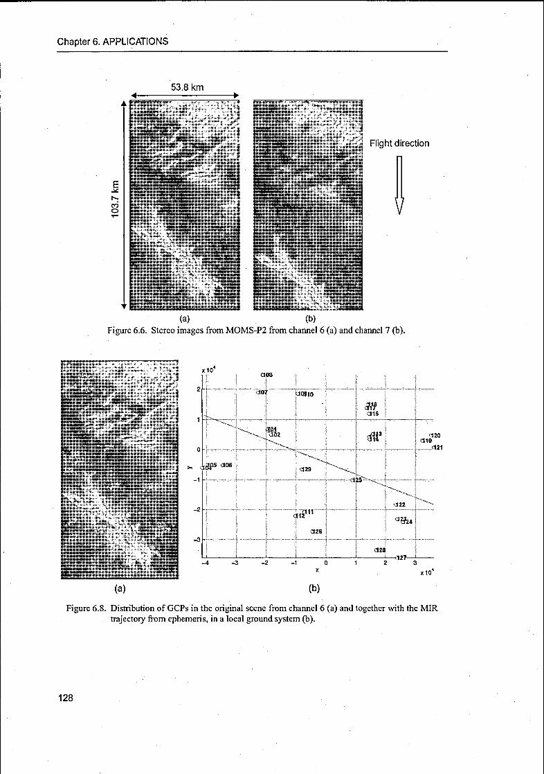
Chapter 6. APPLICATIONS
53.8 km
E
N.
COO
Flight direction
V
(a) (b)
Figure 6.6. Stereo images from MOMS-P2 from channel 6 (a) and channel 7 (b).
x10cioa
2«J07 <3<mo
1 *
016
m3
'
CM9
0 ' "-Ns^ -a
>• < ,jp5 J06C129 ~~^-~
-1 C(25^"^^K."^^
-2 -
di?11
a26
a22
a%4
"^**~^.
-3
i i ' i i
J28
-^12?—L
321
-2 -1 0
XX10
(b)
Figure 6.8. Distnbution of GCPs in the original scene from channel 6 (a) and together with the MIR
trajectory from ephemeris, in a local ground system (b).
128
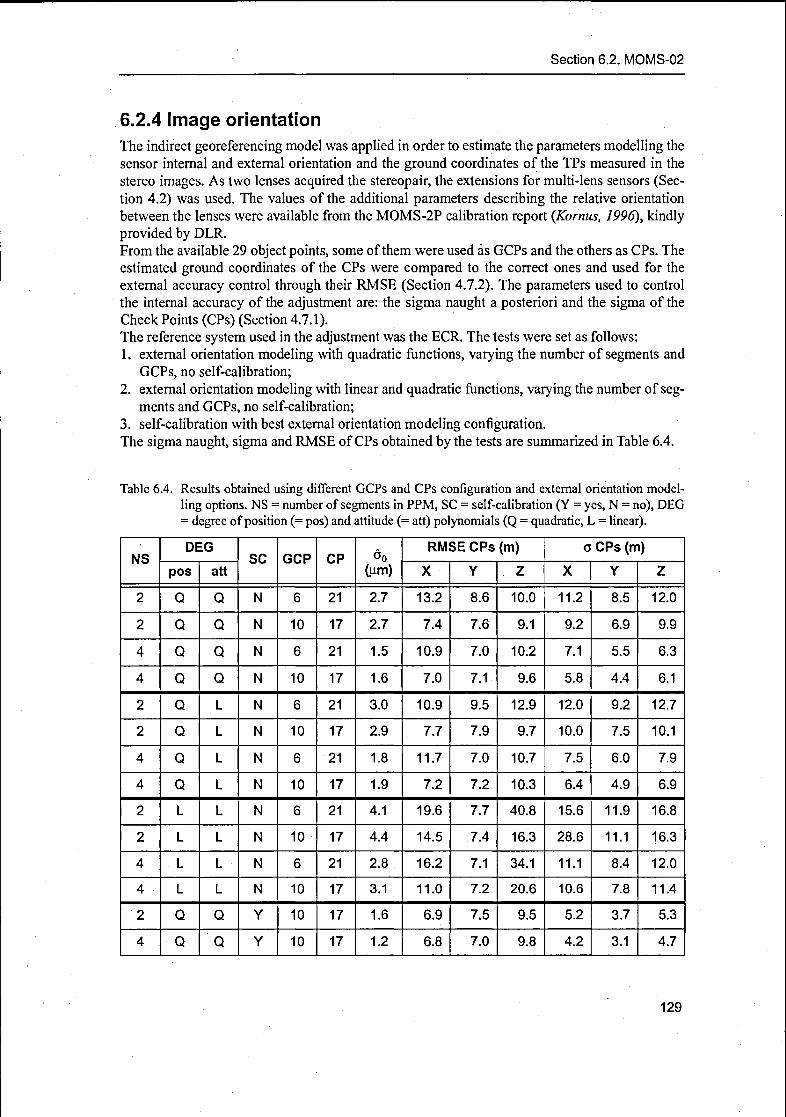
Section 6.2. MOMS-02
6.2.4 Image orientation
The indirect georeferencing model was applied in order to estimate the parameters modelling the
sensor internal and external orientation and the ground coordinates of the TPs measured in the
stereo images. As two lenses acquired the stereopair, the extensions for multi-lens sensors (Sec¬tion 4.2) was used. The values of the additional parameters describing the relative orientation
between the lenses were available from the MOMS-2P calibration report (Kornus, 1996), kindly
provided by DLR.
From the available 29 object points, some ofthem were used as GCPs and the others as CPs. The
estimated ground coordinates of the CPs were compared to the correct ones and used for the
external accuracy control through their RMSE (Section 4.7.2). The parameters used to control
the internal accuracy of the adjustment are: the sigma naught a posteriori and the sigma of the
Check Points (CPs) (Section 4.7.1).The reference system used in the adjustment was the ECR. The tests were set as follows:
1. external orientation modeling with quadratic functions, varying the number of segments and
GCPs, no self-calibration;2. external orientation modeling with linear and quadratic functions, varying the number of seg¬
ments and GCPs, no self-calibration;
3. self-calibration with best external orientation modeling configuration.The sigma naught, sigma and RMSE ofCPs obtained by the tests are summarized in Table 6.4.
Table 6.4. Results obtained using different GCPs and CPs configuration and external orientation model¬
ling options. NS = number of segments in PPM, SC = self-calibration (Y = yes, N= no), DEG
= degree of position (= pos) and attitude (= att) polynomials (Q = quadratic, L = linear).
NSDEG
sc GCP CP ô0(um)
RMSE CPs (m) a CPs (m)
pos att X Y Z X Y Z
2 Q Q N 6 21 2.7 13.2 8.6 10.0 11.2 8.5 12.0
2 Q Q N 10 17 2.7 7.4 7.6 9.1 9.2 6.9 9.9
4 Q Q N 6 21 1.5 10.9 7.0 10.2 7.1 5.5 6.3
4 Q Q N 10 17 1.6 7.0 7.1 9.6 5.8 4.4 6.1
2 Q L N 6 21 3.0 10.9 9.5 12.9 12.0 9.2 12.7
2 Q L N 10 17 2.9 7.7 7.9 9.7 10.0 7.5 10.1
4 Q L N 6 21 1.8 11.7 7.0 10.7 7.5 6.0 7.9
4 Q L N 10 17 1.9 7.2 7.2 10.3 6.4 4.9 6.9
2 L L N 6 21 4.1 19.6 7.7 40.8 15.6 11.9 16.8
2 L L N 10 17 4.4 14.5 7.4 16.3 28.6 11.1 16.3
4 L L N 6 21 2.8 16.2 7.1 34.1 11.1 8.4 12.0
4 L L N 10 17 3.1 11.0 7.2 20.6 10.6 7.8 11.4
2 Q Q Y 10 17 1.6 6.9 7.5 9.5 5.2 3.7 5.3
4 Q Q Y 10 17 1.2 6.8 7.0 9.8 4.2 3.1 4.7
129

Chapter 6. APPLICATIONS
As test 1 concerns, the spacecraft trajectory was divided into 2 and 4 segments (NS=2 and NS=4)ofthe same length, 6 and 10 points were used as GCPs. The corresponding results are reported in
the first four rows in Table 6.4.
We can observe that:
• in all cases RMSE and sigma of CPs are smaller than 1 pixel. The best RMSE in the CPs,achieved with 10 GCP and 4 segments, correspond to 0.4, 0.4 and 0.5 pixels in X, Y and Z
respectively• by increasing the number of segments, the external orientation functions can better fit the real
trajectory, improving the adjustment performance. This is demonstrated by the decrease of the
sigma naught a posteriori and the sigma of CPs. The difference in the CPs RMSE between 2
segments and 4 segments configurations is less than 0.5m, corresponding to 3% of the ground
pixel size
• by increasing the number of GCPs, sigma naught a posteriori remains approximately constant
and the sigma of the CPs decreases, because the system is more stable
• the distribution of the residuals in the GCPs and CPs in Figure 6.9 (a and b) shows that all the
systematic errors are removed.
Test 2 was performed in order to establish if the polynomial degree of the position or attitude
functions could be reduced. The indirect georeferencing model was run using again 6 and 10
GCPs and 2 and 4 segments for the PPM. For the external orientation modelling, quadratic func¬
tions for the position and linear functions for the attitude (pos = Q, att = L, second group ofrows
in Table 6.4) and linear functions for both position and attitude (pos = L, att = L, third group of
rows in Table 6.4) were tested. The comparison between the results achieved with quadratic and
linear functions show that the sigma naught a posteriori, the sigma and RMSE of CPs increase,
demonstrating that, at least with this particular dataset, quadratic functions for both position and
attitude are recommended, because they fit better the true trajectory and produce the best results.
Finally a self-calibration was applied using the configuration with 10 GCPs and 17CPs, 2 and 4
trajectory segments and quadratic external orientation functions (pos = Q, att = Q). The flexibil¬
ity of the software allows the user to fix any unknown parameters to the wished values with
pseudo-observations (Section 4.5.2.2). Due to the very high correlation between the internal and
external orientation, for each test with self-calibration the external orientation parameters were
fixed to the values estimated in the same configuration without self-calibration and only the self-
calibration parameters were estimated. In order to determine only the additional parameters
(APs) of interest, the tests were repeated with different self-calibration configurations. In the first
run all the self-calibration parameters were let free and their mean values, sigma and correlations
were analyzed. The unpredictable or correlated parameters were fixed to constant values. The
estimated APs were: 9 for each line, plt p2, kt and k2 for both lenses. Among them, 9 and k2resulted insignificant. The maximum effect of the other parameters for both lenses are computedfor the pixels on the border (u = 1488) according to the Equations in Section 4.4. The maximum
values are:
forPf. Ax= 0.010mm (1 pixel)for p2: Ay= 0.010mm ( 1 pixel)for k{. Ay= 0.020mm (2 pixels)
Comparing the values in Table 6.4 corresponding to NS = 2 and NS = 4, pos= Q, att = Q,
GCP=10, CP = 17, without (SC = N) and with self-calibration (SC = Y), it can be observed that
using self-calibration the system converges easier to the solution: the sigma a posteriori of the
full adjustment reduces considerably together with the sigma of the CPs. The RMSE differs few
130

Section 6.2. MOMS-02
centimeters, with smaller values inXand Fand larger values in Z (maximum 40cm). Consideringthe ground pixel size of 18.0m, these RMSE differences are not significant. The final RMSE dis¬
tribution with self-calibration is shown in Figure 6.9 (c and d).
Apart of the tests where both the position and attitude are modelled with quadratic functions, the
differences between the RMSE and the standard deviation of the CPs vary between 0.5m and 4m.
Even if these values represent a small fraction of the pixel size (0.45 of the pixel size), they show
that the theoretical (expected) accuracy is slightly better than the achieved one. This fact can be
explained with a wrong weight assignment to the image and ground coordinates of the objectpoints. In fact in our software the same weight is used for all the points. If a point is measured
with a different accuracy, it may negatively affect the adjustment process.
Residuals In XY «»* Residuals In Z
• Residuals In XY ,,„< Residuals In Z
Figure 6.9. Residuals distributions in XY (on the left side) and Z (on the right side) using quadratic func¬
tion for position and attitude (pos = Q, att = Q), NS = 2,10 GCPs (marked with triangles) and17 CPs (marcked with circles), before (top) and after (bottom) self-calibration.
131

Chapter 6. APPLICATIONS
6.2.5 Summary and conclusions
In this Section the processing of a MOMS-P2 stereopair has been presented. The work included
the data preparation (radiometric preprocessing, point measurement, external orientation analy¬sis) and the orientation with our rigorous sensor model. As the accuracy of the external orienta¬
tion was not accurate enough for high precision mapping, the indirect georeferencing model was
used in order to estimate the sensor orientation parameters and the ground coordinates of the tie
points (GCPs and TPs). The model was run in the ECR system. Different GCPs distributions and
PPM configurations (number ofsegments, polynomial degree) have been tested with and without
self-calibration. The correct parameters for the focal length and principal points displacementwere available from the laboratory calibration report (Kornus, 1996).The results obtained in the internal and external accuracy, summarized in Table 6.4, show that
using quadratic functions for the position and attitude modelling and a minimum of 6 GCPs sub-
pixel accuracy in the CPs can be achieved. By increasing the number ofGCPs to 10, residuals of
7.0m inX, 7.1m in Y and 9.6m in Z, corresponding to 0.4, 0.4 and 0.5 pixels respectively, can be
achieved in the CPs. Using self-calibration, the RMS values do not change significantly and the
standard deviations ofthe CP ground coordinates reduce ofabout 1.5m. We can conclude that for
this dataset if the focal length and principal point displacement values available from the labora¬
tory calibration are used, the self-calibration does not give a significant improvement of the final
results.
In order to evaluate the performance of our model, the same stereopair has been oriented usingSpotcheck+ software by Kratky Consulting (Kratky, 1989). According to Kratky's approach, the
satellite position is derived from known nominal orbit relations, while the attitude variations are
modelled by a simple polynomial model (linear or quadratic). For self-calibration two additional
parameters are added: the focal length and the principal point correction. The exterior orientation
and the additional parameters are determined in a general formulation by least-squares adjust¬ment. This model has been used for the orientation of SPOT (Baltsavias and Stallmann, 1992),MOMS-02/D2 (Baltsavias and Stallamann, 1996b), Landsat TM and JERS-1/OPS and was also
investigated and extended in Fritsch and Stallmann, 2000. Using 10 GCPs (the same points used
in our tests) and modelling the attitude with quadratic functions, the sigma naught a posterioriwas 2.2u.m and the residuals achieved in 19 CPs were 5.2m in East, 4.4m in North and 11.1m in
height in the Gauss-Kriiger coordinate system (Poli et al, 2000). The corresponding values
achieved with our model in Gauss-Kriiger system are 5.5m, 4.3m and 11.3m for East, North and
height. The results obtained by the two models are very similar; taking into account the groundresolution (18m), the differences are not significant. In both cases the modelling of the attitude
with quadratic functions gave better results and the correction of the internal orientation parame¬
ters (in particular the focal length and principal point position) using the laboratory calibration or
the self-calibration, is recommended.
At the Institute for Photogrammetry (IFP) of the University of Stuttgard, Spotcheck+ was used
for the orientation of other MOMS-P2 scenes acquired again on 14th March 1997 along the track
T083C few seconds after our scenes (scenes 27-30). Using 10 GCPs, RMS values of 11.2m,
11.4m and 13.7m were achieved in X, Yand Z for 24 CPs. The points were measured in 1:25,000scale digital topographic maps with an accuracy of 0.5 pixels in image space and 8.5m in object
space. Compared to these results, the accuracy achieved with our model is satisfying.In conclusion, we have shown that with sub-pixel accuracy can be achieved in the orientation of
MOMS-P2 with our rigorous model, in accordance with the performance of other commercial
software.
132

Section 6.3. SPOT-5/HRS
6.3 SPOT-5/HRS
In 2003 the Institute of Geodesy and Photogrammetry (IGP), ETH Zurich, joined the HRS Scien¬
tific Assessment Program (HRS-SAP), organized by CNES and ISPRS. This initiative,announced in Denver in 2002 at the ISPRS Commission I Symposium and concluded in Istanbul
at the XX ISPRS Congress, had the aim to investigate the potential of SPOT-5/HRS sensor for
DEM generation. The aim was to help CNES to improve its future Earth Observation systemsand all users to better know and trust the accuracy and quality of the HRS instrument and the
derived DEM. IGP joined the Initiative as Co-Investigator, that is, it processed the data provided
by one of the Principal Investigators, generated two DEMs with two different orientation meth¬
ods, compared them to the reference DEMs and produced a quality report. The dataset given to
IGP for the processing was the number 9, over the Chiemsee Lake, in Germany. For more infor¬
mation about the Initiative see Baudoin et al, 2004.
SPOT-5 is the latest satellite of SPOT (Satellite pour l'Observation de la Terre) constellation of
CNES, France. The SPOT system has been operational since 1986 when SPOT-1 was launched.
SPOT-2 was placed in orbit in January 1990, followed by SPOT-3 in September 1993, SPOT-4
in March 1998 and SPOT-5 in May 2002. At present three satellites are in orbit: SPOT-2, SPOT-
4 and SPOT-5, operated by Spotlmage. The SPOT system is designed to achieve optimum image
quality in terms of resolution and solar illumination and to respond quickly to the user requests.The satellites fly over the Earth at an altitude of 822km at the Equator. The orbit is circular and
near polar to maintain a constant resolution of any point on the globe and is phased, so that a sat¬
ellite passes over the same point every 26 days. The satellites thus repeat the same ground tracks
with the maximum distance at the Equator of 108 km. The instruments carried onboard the satel¬
lites acquire images at different resolution and spectral coverage and provide the users with a
large variety of products. The spectral bands and resolutions of the sensors carried on SPOT sat¬
ellites are summarized in Table 6.5.
Table 6.5.SPOT satellite spectral bands and resolutions.
Satellite Sensor Electromagnetic spectrum Pixel size (m) Spectral bands (u.m)
SPOT-5
HRS Panchromatic 10(5)a 0.49 - 0.69
HRG
Panchromatic 5 (2.5)a 0.48 - 0.71
B1: green 10 0.50 - 0.59
B2: red 10 0.61 - 0.68
B3: near infrared 10 0.78 - 0.89
B4: mid infrared (MIR) 20 1.58-1.75
SPOT-4 HRVIR
Panchromatic 10 0.61 - 0.68
B1: green 20 0.50 - 0.59
B2: red 20 0.61 - 0.68
B3: near infrared 20 0.78 - 0.89
B4: mid infrared (MIR) 20 1.58-1.75
SPOT-1
SPOT-2
SPOT-3
HRV
Panchromatic 10 0.51 - 0.73
B1: green 20 0.50 - 0.59
B2: red 20 0.61 - 0.68
B3: near infrared 20 0.78 - 0.89
a.after resampling
133

Chapter 6. APPLICATIONS
6.3.1 Sensor descriptionWithin the SPOT constellation, SPOT-5 is the most innovative satellite. The new HRG (HighResolution Geometry) instrument, derived from the HRVIR instrument on SPOT-4, offers up to
2.5m resolution in panchromatic mode in across-track direction. Moreover the new HRS (HighResolution Sensor), used in this work, allows the acquisition of stereo images in along-trackdirections, using two instruments pointing about 20° forward and backward the flight direction
(Figure 6.10). Each scene acquired by HRS has a field ofview of 120km, with a ground resolu¬
tion of 10m across and 5m along the flight direction. The 5m resolution is achieved after resam¬
pling. The technical data of the HRS instrument are summarized in Table 6.6.
Table 6.6 HRS technical data.
Mass 90kg
Power 128W
Dimensions 1m x 1.3m x 0.4m
Field of view 8°
Focal length 0.580m
Detectors per line 12,000
Detector size 5.7pm
Integration time per line 0.752ms
Forward/aft viewingangle relative to vertical
2tf
Spectral range (PAN) 0.49 pm - 0.69 um
Ground sampledistance:
-across track
-along track
10m
10m(5m)a
Signal-to-noise ratio >120
Figure 6.10 Acquisition of SPOT-5 HRS.
a after resampling
6.3.2 Data descriptionThe dataset number 9 provided during the ISPRS-CNES Initiative covered partly South of Ger¬
many and partly Austria. The following data have been received from CNES and DLR Berlin:
• Stereo images from SPOT-5/HRS acquired on 1st October 2002 in the morning over an area of
approximately 120km x 60km
• Metadata file for each scene. The files contain the time acquisition and image location, the sen¬
sor position and velocity measured by DORIS system every 30 seconds, the attitude and angu¬
lar speeds from star trackers and gyros at 12.5 seconds interval, with respect to the local orbital
coordinate frame, the sensor geometric (detectors looking angles) and radiometric calibration
• Description of exact position of 81 object points in Germany, measured with surveying meth¬
ods. The coordinates were given in Gauss-Kriiger system• 4 DEMs in Southern Bavaria (Prien, Gars, Peterskirchen, Taching) created from laser scanner
data with a pixel spacing of5m and an overall size ofabout 5km x 5km. The height accuracy is
134

Section 6.3. SPOT-5/HRS
better then 0.5m
• 2 DEMs in the area of Inzell (total: 10km x 10km, 25m spacing). The first one, called 5-1, was
derived from laser scanner data (northern part, height accuracy better then 0.5m) and the other
one, called 5-2, was derived from contour-lines 1:10,000 (southern part, height accuracy of
about 5m)• A large coarse DEM (area of Vilsbiburg, 50km x 30km) with 50m spacing and height accuracy
of about 2 meters, derived by conventional photogrammetric and geodetic methods; only a
small part of this DEM is covered in the scenes.
An overview of the characteristics ofthe reference DEMs and their location in the image area are
given in Table 6.7 and Figure 6.11.
The SPOT stereo scenes had a size of 12,000 pixels across the flight direction and 12,000 pixelsalong the flight direction, with a ground resolution of 10m (across-track) x 5m (along-track). The
time difference between their acquisition was 90s. The scenes were a level 1A product, with radi¬
ometric correction of the distortions due to differences in sensitivity of the elementary detectors
of the viewing instruments. In the next paragraphs the work applied on the SPOT scenes is
described. After the scene orientation, a DEM was generated and compared to the reference data.
Table 6.7.Main characteristics ofthe reference data sets.
DEM Location DEM
SpacingSource DEM
SizeHeight
Accuracy
1 Prien 5mx5m Laser Scanner 5km x 5km 0.5m
2 Gars 5mx5m Laser Scanner 5km x 5km 0.5m
3 Peterskirchen 5mx5m Laser Scanner 5km x 5km 0.5m
4 Taching 5mx5m Laser Scanner 5km x 5km 0.5m
5-1 Inzell-North 25m x 25m Laser Scanner 10km x 1.3km 0.5m
5-2 Inzell-Sourth 25m x 25m Contour lines 10km x 7.7km 5.0m
6 Vilsbiburg 50m x 50m Photogrammetry 50km x 30km 2.0m
6.3.3 PreprocessingThe images have been radiometrically enhanced with Wallis filter (Section 5.3.1). For each scene
the acquisition time of each image line was calculated from the acquisition time of the central
line and the scanning interval time contained in the metadata files, according to Equation 3.19.
The ground control points were measured in the images using the description files provided byDLR. From the 81 points, only 41 have been measured in the images. The other points were not
visible in the images or could not be recognized due to the resolution of the images. Figure 6.12
shows the point distribution in one of the two scenes. A digital map at 1:50,000 scale by Topo50
(Bayerische Vermessungsverwaltung, 2004) was used to recognize the main ground features
(streets, rivers, lakes, forests, ...) and locate the points. The accuracy of the object coordinates
was within few centimeters, as they were measured with topographic methods.
The exact image coordinates have been measured with sub-pixel accuracy with unconstrained
Multiphoto Least Squares Matching available at IGP (Baltsavias, 1991). We supposed a mea¬
surement accuracy of 0.5 pixels. Figure 6.13 shows an example of point measurement with
matching.
135
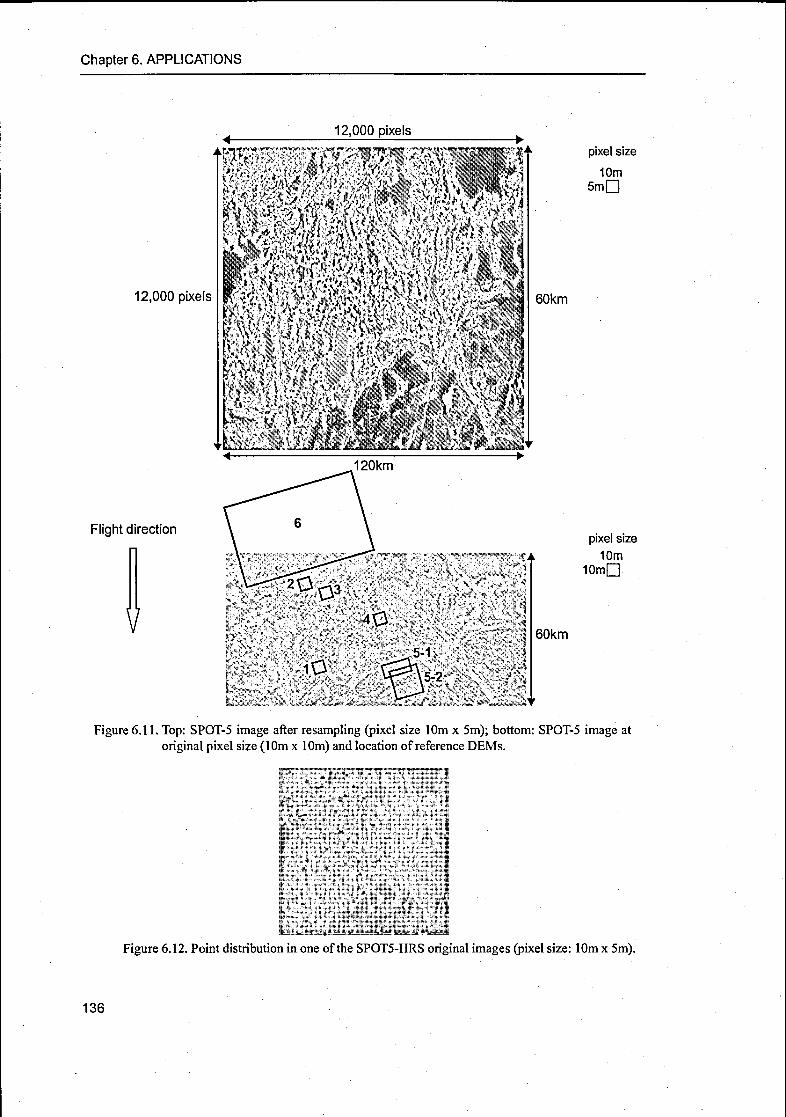
Chapter 6. APPLICATIONS
12,000 pixels
12,000 pixels
Flight direction
V
60km
pixel size
10m
5mD
pixel size
10m
lOmQ
60km
Figure 6.11. Top: SPOT-5 image after resampling (pixel size 10m x 5m); bottom: SPOT-5 image at
original pixel size (10m x 10m) and location of reference DEMs.
Figure 6.12. Point distribution in one ofthe SPOT5-HRS original images (pixel size: 10m x 5m).
136

Section 6.3. SPOT-5/HRS
iMiwauaiWM
Pli«* CMfKapMSt
4S01KIM D0BT4S« OK tWHOnm
8038 060 00
»SOt 80 11 (5 11
Figure 6.13. Identification of object points in SPOT-
5/HRS stereopairs: description file (left)and least-squares matching (right).
6.3.4 Image orientation
The direct georeferencing approach was used in order to test if the camera calibration and the
ephemeris available in the metadata files were accurate enough for high precision mapping. The
information on the internal orientation was given through the viewing angles of each detector
expressed within the sensor coordinate frame. From these data the position ofeach detector in the
focal plane was computed as explained in Section 5.2. The position and velocity vectors were
used for the estimation of the sensor attitude in the ECR system (Equation 3.16). Then the posi¬tion and attitude were interpolated with cubic splines for the acquisition times of the image lines.
A forward intersection was applied to calculate the ground coordinates of the object points. The
resulting coordinates were compared to the correct values and the RMSE were evaluated. The
results showed a large systematic error both in planimetry (2-3 pixels) and in height (~3 pixels).Therefore the indirect georeferencing model was required for the internal and external orienta¬
tion refinement.
The object coordinates were transformed into the ECR system, which was used as reference sys¬
tem for the geometric processing. From the available 41 points, a group of them was used as
GCPs and the remaining as CPs. The GCPs were chosen in order to have a good distribution. The
a priori standard deviation of the GCPs was 3m. The tests have been carried out with different
input configurations, in this order:
1. external orientation modeling with quadratic functions, varying the number of segments and
GCPs configurations, no self-calibration
2. external orientation modeling with linear and quadratic functions, best GCPs configurationand best trajectory segments, no self-calibration
3. self-calibration with best external orientation modeling configuration.
As already encountered with MOMS-02, the PPM gave better results with quadratic functions,
than with linear ones. Using linear functions, the RMS and standard deviation values were close
to 1 pixel. The RMSE and the sigma of the CPs and the sigma naught of the adjustment obtained
with quadratic functions without and with self-calibration are reported in Table 6.8.
137

Chapter 6. APPLICATIONS
Table 6.8. Results obtained using different GCPs and CPs configuration and external orientation model¬
ling options. X, Y and Z refer to ECR system. NS = number of segments in PPM, SC = self-cal¬
ibration (Y = yes, N= no).
NS SC GCP CP à0(um)
RMSE CPs (m) a CPs(m)
X Y Z X Y Z
2 N 6 35 2.7 5.6 8.7 9.4 5.2 8.5 3.7
2 N 12 29 2.9 5.5 7.2 9.2 4.0 7.2 3.1
4 N 6 35 2.6 5.5 8.5 9.2 5.2 8.4 3.6
4 N 12 29 2.8 5.4 7.1 9.0 4.0 7.2 3.1
2 Y 6 35 1.1 3.8 6.9 3.9 2.2 3.2 3.5
2 Y 12 29 1.2 3.7 6.1 3.5 1.7 2.4 2.6
4 Y 6 35 0.8 3.9 6.8 3.7 1.9 2.9 2.8
4 Y 12 29 0.9 3.7 6.0 3.3 1.5 2.3 2.5
Taking into account the results achieved without self-calibration (first 4 rows ofTable 6.8), it can
be seen that increasing the number ofPPM segments the adjustment converges better (smaller ô0and ct ofthe CPs) and the RMS values remain quite constant. As expected, the use ofmore GCPs
gives better solutions, in terms of internal and external accuracy. The RMSE sizes and distribu¬
tions in the object space evidence that if only the external orientation is modelled, the systematicerrors are not completely removed. In the top of Figure 6.14 an example of RMSE distribution
(12 GCPs and 29 CPs) is shown.
In the next step the self-calibrating bundle adjustment was used. Each adjustment with self-cali¬
bration was run with the external orientation parameters fixed to their values estimated without
self-calibration. The results are reported in the last 4 rows of Table 6.8 (SC = Y). By a visual
analysis, Figure 6.14 shows the reduction of the systematic behavior in the RMSE distribution.
Also the quantitative comparison between the RMSE and ct values of the CPs and the c0 before
and after the self-calibration confirms an improvement both in the internal and external accuracy
of the adjustment. The significant self-calibration parameters were the symmetric radial distor¬
tion (through kj) and the scale in y direction (sy), with the focal length fixed. These parameterswere different for each lens and their effect could not be compensated during the estimation of
the external orientation parameters only, which is unique for the entire system. The maximum
effects of the estimated parameters for each lens are calculated for the pixels on the image bor¬
ders (u = 6,000) with Equation 2.15 for kj and Equation 2.17 for sy They are reported in Table
6.9.
Table 6.9. Maximum errors in lenses 1 (forward) and 2 (backward) caused by lens distortion. The errors
are expressed in mm and in pixels.
Parameter Lens 1 Lens 2 Ay, (mm) Ay2 (mm) Ay, (pixels) Ay2 (pixels)
ki -5.7*10"7 -7.7*10'7 -0.020 -0.030 3.6 5.3
sy -5.1*10^ -4.8*10"4 -0.020 -0.020 3.6 3.6
138

Section 6.3. SPOT-5/HRS
«10S Residuals In XY
6345
'!
1J .! 5m I!
•- —
6.34
i'v1
\ t J
5.335
! .1.. »
•
! i' :
6.33'
- — - * - -t — -
1125
6.31i l
- v ;- -
• * -
t
8 315 " " ._.,... ï *
T
6.31
1303 • " i i /.
5.3
S 295 :- - - -
]
4 i
4.32 4SI 4 54 4 9S
«»' Residuals In XY
1345
6 34
1339
-
A
1 P
• •
S 33
«L„
•*-
6,325 «C -
532
6,316 . *,
•> «
.*-
^A (
5 31
6.306
"V"
> - - -
"' -\ - *^~*.
»
- \ .. p - .
i;
6.3
5.Z95
i
! •
A.
- • -
4 5 4 51 455 4 55
.«• Residuals In Z
1.345 - 4 i > i will-
5.34
6335
_..
A
•
4
t
t
t
Ài
•
- -
533 ... . -1-
-
'-
< •- - - » - '
6325 - ... *
i , Xï. -
!- . -
132 " *-- *•
*l 1 ..
6.31! -" ~ • _
«
f;
- ' - -
5 31•
i.•
*-
t •
5.305 • i- * f
•
•
13
5.295 •
t
* '
"
T.**•
t
!•
' *
«101 Residuals in Z
5.343
5.34
5.335
L*t
•
*
«
T•
- t
A
•
i
6.33 i"
^-
t • '
, f • >
5.3» i ..
"*. i* ..
5.32 i
A
•
**
J. !
5 316 — -
•
»•
[~
"I...
5.31*
t
• ; «
S 305 .„ ••• - ...
•
_ • — i »
•
î-
S-3
B195 ' . » u
•
A
T•
. t
\ •
t
r
i
4» 4.M
Figure 6.14. Residuals in planimetry and height (Gauss-Krüger system) for all object points in the con¬
figuration with 2 segments in the PPM and 8 GCPs (marked with triangles). On the top are
the results without self-calibration, on the bottom with self-calibration.
6.3.5 DEM generationFor the matching and DEM generation, algorithms and software packages developed in our
group for airborne or spaceborne linear array sensors (Grün et al, 2004, Zhang and Grün, 2003,Grün and Zhang, 2002a) have been used. The approach takes into account the characteristics of
the linear array image data for matching and automatic DEM extraction.
6.3.5.1 Image matching
The image matching used in this case study was implemented in SAT-PP software (Zhang and
Grün, 2003). The algorithm, based on the Multi-Photo Geometrically Constraint (MPGC)
matching (see Grün, 1985, Grün and Baltsavias, 1988, Baltsavias, 1991), is a combination of
feature point, edge and grid point matching and can achieve sub-pixel accuracy for all the
matched features. Figure 6.15 shows the matching process scheme.
139

Chapter 6. APPLICATIONS
Images and Orientation Data
Image Pre-processing & ImagePyramid Generation
Feature Point
Matching Edge MatchingGrid Point
Matching
GeometricallyConstrained
Candidate Search,
Adaptive MatchingParameter
Determination
DSM (intermediate)Viwmuinauwn or reature poims, gnu poioia emu
edges
1Modified Muäi-Image Geometrically
Constrained Matching (MPGC)
s *
Final DSM
Figure 6.15.Workflow ofthe image matching procedure (Zhang and Grün, 2003).
After the pre-processing of the imagery and production of the pyramids, the matches of three
kinds of features, i.e. feature points, grid points and edges, are found progressively in all pyramidlevels starting from the low-density features on the images with the lowest resolution. A Triangu¬lar Irregular Network (TIN) based DEM is constructed from the matched features on each level
of the pyramid and is used in turn in the subsequent pyramid level as approximation for the adap¬tive computation of the matching parameters. Finally the modified MPGC matching is used to
achieve more precise results for all the matched features on the original resolution level (level 0)and to identify some inaccurate and possible false matches. The raster DEMs are interpolatedfrom the original matching results using DTMZ software.
The main characteristics of the matching procedure are:
• It is a combination of feature point, edge and grid point matching. The grid point matching pro¬
cedure uses relaxation-based relational matching algorithm and can bridge-over the non- and
little-texture areas through the local smoothness constraints. The matched edges are introduced
to control the smoothness constraints and preserve the surface discontinuities.
• The adaptive determination of the matching parameters results in higher successful rate and
less false matches. These parameters include: the size of the matching window, the searchingdistance and the threshold values for cross-correlation and MPGC (Least Squares matching).For instance, the procedure uses a smaller matching window, larger search distance and a
smaller threshold value in rough terrain area and vice versa. The roughness ofthe terrain can be
computed from the approximate DEM on higher levels of image pyramid.• Object edges are important for preserving the surface discontinuities. A robust edge-matchingalgorithm, which uses the adaptive matching window determination through the analysis of the
image contents and local smoothness constraints along the edges, is combined into the proce¬
dure.
• Together with matched point features, edges (in 3D) are introduced as break-lines when a TIN-
based DEM is constructed. It provides a good approximate for matching on the next pyramid
140
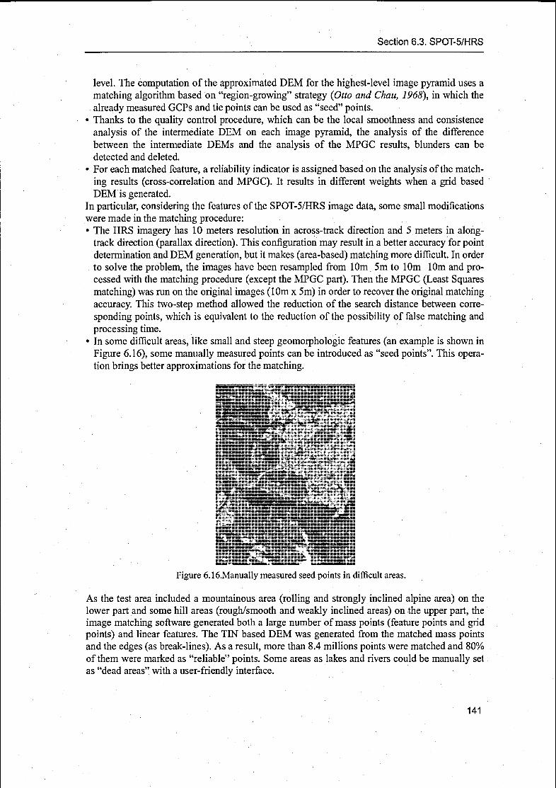
Section 6.3. SPOT-5/HRS
level. The computation of the approximated DEM for the highest-level image pyramid uses a
matching algorithm based on "region-growing" strategy (Otto and Chau, 1968), in which the
already measured GCPs and tie points can be used as "seed" points.• Thanks to the quality control procedure, which can be the local smoothness and consistence
analysis of the intermediate DEM on each image pyramid, the analysis of the difference
between the intermediate DEMs and the analysis of the MPGC results, blunders can be
detected and deleted.
• For each matched feature, a reliability indicator is assigned based on the analysis of the match¬
ing results (cross-correlation and MPGC). It results in different weights when a grid based
DEM is generated.In particular, considering the features of the SPOT-5/HRS image data, some small modifications
were made in the matching procedure:• The HRS imagery has 10 meters resolution in across-track direction and 5 meters in along-track direction (parallax direction). This configuration may result in a better accuracy for pointdetermination and DEM generation, but it makes (area-based) matching more difficult. In order
to solve the problem, the images have been resampled from 10m 5m to 10m 10m and pro¬
cessed with the matching procedure (except the MPGC part). Then the MPGC (Least Squares
matching) was run on the original images (10m x 5m) in order to recover the original matching
accuracy. This two-step method allowed the reduction of the search distance between corre¬
sponding points, which is equivalent to the reduction of the possibility of false matching and
processing time.
• In some difficult areas, like small and steep géomorphologie features (an example is shown in
Figure 6.16), some manually measured points can be introduced as "seed points". This opera¬
tion brings better approximations for the matching.
Figure 6.16.Manually measured seed points in difficult areas.
As the test area included a mountainous area (rolling and strongly inclined alpine area) on the
lower part and some hill areas (rough/smooth and weakly inclined areas) on the upper part, the
image matching software generated both a large number of mass points (feature points and grid
points) and linear features. The TIN based DEM was generated from the matched mass pointsand the edges (as break-lines). As a result, more than 8.4 millions points were matched and 80%
of them were marked as "reliable" points. Some areas as lakes and rivers could be manually set
as "dead areas" with a user-friendly interface.
141

Chapter 6. APPLICATIONS
6.3.5.2 DEM generation
The ground coordinates of the 8.4 millions points measured in the images were estimated using a
forward intersection algorithm (Section 4.8). The resulting coordinates, in the ECR Geocentric
system, were transformed into Gauss-Kriiger system in order to be compared to the reference
DEMs. The 3D point cloud was transformed into a regular grid with 20m x 20m grid space with
DTMZ software. In Figure 6.17 the generated DEM is shown.
6.3.6 Comparison
The generated DEM has been compared to the reference DEMs provided by the HRS-SAP. The
main characteristics (location, spacing, source, size and height accuracy) ofthe reference data are
shown in Table 6.7. The coordinate system used for the comparison is the Gauss-Kriiger systemZone 4 with Bessel-ellipsoid and Potsdam datum.
Two accuracy tests have been performed, in 2.5D and 3D respectively. In the first test the differ¬
ences between the heights ofthe reference DEMs and the corresponding height interpolated from
our DEMs have been computed (2.5D). The limit of this approach is that it is highly influenced
by the errors of the surface-modelling algorithm. Figure 6.18 illustrates the concept with a step
profile: even if the measurements (point P) are accurate, the modeled profile cannot follow the
true one. Consequently if the terrain height is compared, in presence of the step, a large differ¬
ence (Ah) may be measured. For that reason the computation of the 3D orthogonal distance
between the surfaces (distance d in Figure 6.18) is theoretically more correct. Therefore the sec¬
ond accuracy test is based on the evaluation of the normal distance (3D) between our measure¬
ments (3D point cloud) and the reference DEMs. This test is fundamental in this case studywhere steep mountains (like Alps) are present. The results of the two tests are reported in Tables
6.10 and 6.12.
Ah
\
\
\
yad
Figure 6.18. Modelling problems. The true profile is the full black line, the modelled profile is the
dashed line.
6.3.6.1 Accuracy tests on the terrain height (2.5D)
This analysis has been carried out using different tools developed at IGP. The results obtained
comparing all the points are reported in Table 6.10 (3rd to 6th column). It can be observed that the
accuracy of the measured DEM is more or less on 1-2 pixels level, depending on the terrain type.
As expected, a better accuracy is achieved in smooth and flat areas, while in the mountainous
area (DEMs 5-1 and 5-2) the RMSE are larger. In all datasets some blunders which failed to be
detected are still present. In the reference datasets 5-1 and 5-2 some blunders are even above
100m, with a bias up to 1.0 pixels. Apart from the results of reference DEM 6, all the biases are
negative, indicating that the generated DEM is higher than the reference ones. For further analy¬
sis, the frequency distribution of the height differences is shown in the second column of Table
6.11 (DEM 6 is missing because only a small portion was covered by the scenes). In the fre¬
quency distribution of the height differences two peaks occur, one located around value 0.0 and
142

Section 6.3. SPOT-5/HRS
Figure 6.17. DEM generated from 8.4 millions points with a forward intersection using the esti¬
mated internal and external orientations. The black holes represent "dead areas".
143

Chapter 6. APPLICATIONS
the other one around a negative value (ca. 8m). The relative frequency values could be correlated
to the percentage ofpresence of trees. In fact from a qualitative analysis of the error distribution,we noticed that the negative height difference (the green areas) have the same clustering of the
areas covered by trees, while the open areas have small height difference values. Then the bias
located at -8m could be mainly caused by the trees. This is a main problem for extracting a DEM
by using the optical imaging systems, as the light cannot penetrate the vegetation. In fact the gen¬
erated digital model does not represent the terrain (DEM or DTM), but the surface (DSM) visible
by an optical instrument, including houses, trees, bushes and so on. In order to verify that our
results where affected by the influence of the trees, the areas covered by trees have been manu¬
ally removed from the images and the accuracy tests have been repeated. The percentage of
removed points is 25, 26, 17, 28, 75 and 71 for DEM 1, 2, 3, 4, 5-1, 5-2 and 6 respectively. The
results obtained by the new accuracy tests are shown in Table 6.10 (last 4 columns). As expected,the negative bias was reduced. This is also graphically confirmed by the new frequency distribu¬
tion reported in the third column ofTable 6.11. The analysis of the frequency distributions shows
that in steep mountain areas (DEMs 5-1 and 5-2) there are positive height-difference values.
They are probably caused by the presence of blunders or by the local smoothness constraints
used in the matching algorithm. In fact these constraints smooth out some steep and small fea¬
tures of the mountain areas under the condition that there are not enough extracted and matched
linear features.
Table 6.10.2.5D comparison between reference and generated DEMs, with and without trees. For each
comparison, the maximum, minimum and mean difference and the RMSE are reported.
DEM
Name
N. of
Matched
Points
Max
(m)Min
(m)Mean
(m)RMSE
(m)Max
(m)Min
(m)Mean
(m)RMSE
(m)
with trees without trees
1 35448 22.1 -26.1 -4.0 6.2 13.8 -23.6 -3.0 5.4
2 32932 37.7 -37.1 -3.0 5.5 32.3 -31.2 -1.8 3.9
3 33450 19.7 -17.8 -1.9 4.0 19.6 -14.1 -2.3 3.4
4 32067 11.5 -21.7 -3.8 5.2 9.5 -17.1 -2.8 3.9
5-1 10327 27.1 -36.8 -6.7 9.5 16.1 -23.3 -3.4 5.3
5-2 71795 130.3 -86.1 -5.7 11.3 104.7 -55.5 -4.0 7.4
6 130558 22.7 -19.0 1.1 3.8 21.9 -14.6 -0.7 3.9
144

Section 6.3. SPOT-5/HRS
Table 6.11.DEM accuracy analysis, first column: Name of reference dataset; second column: frequencydistribution of the height-differences for all points; third column: frequency distribution of the
height-differences for points after trees removal.
DEM Histogram for all pointsHistogram without
points on trees
1
PIH2
HB3
n4
H^^^B^^B^^rAv' Vfl^^^H^B
5-1
MpHk ^RBB^nflaVb^b^b^b^bP I^b^b^bBI
5-2
B^B^Hffit; ^ \»bVbVbV
B^B^B^B^B^BT^^B^B^B^B^B^I
145

Chapter 6. APPLICATIONS
6.3.6.2 Accuracy tests based on the orthogonal distances
This analysis has been carried out with the commercial software Geomagic Studio v.4.1 by Rain¬
drop Geomatic (Geomagic Studio, 2004). This software can compare a 3D surface (in our case
generated from the reference DEMs) and a point cloud (in our case, our 3D point cloud). It calcu¬
lates the normal distance between each triangle ofa surface and the closest point ofthe cloud. As
output, the software gives the number of points compared («), the mean (u) and absolute maxi¬
mum distance and the standard deviation (a). The sign of the mean values has been changed to
be homogeneous with the 2.5D results previously shown. From these elements the RMSE is cal¬
culated as:
RMSE2 = —-a2 + p.2 (6.1)
The results are reported in Table 6.12. Comparing these results with those obtained in the 2.5D
comparison, it can be seen that both the mean distance and standard deviation are now reduced in
all datasets. This demonstrates that part of the errors estimated with the 2.5D accuracy tests may
be due to modelling errors or to the planimetric errors. Again, the larger errors have been found
in mountainous areas (DEM 5-2), while in flat terrains the accuracy of the generated DEMs is
very good. The mean values and RMSE obtained by the 2.5D and 3D tests are graphically sum¬
marized in Figure 6.19.
From both the 2.5D and 3D quality analysis the average error between the generated and the ref¬
erence DEMs is around 1-2 pixels (2.5D analysis) and up to slightly more than 1 pixel (3D anal¬
ysis), depending on the terrain type. The best results were achieved in smooth and flat areas,
while in mountain areas some blunders even exceeded 100 meters. In conclusion, this investiga¬tion demonstrated the possibility to apply the developed model on HRS scenes and the high
potential of the scenes themselves for DEM generation.
Table 6.12.3D comparison between generated and reference DSMs.
DEM
Maximum
Difference
(m)
Mean
Difference
(m)
Standard
deviation (m)RMSE(m)
1 16.9 -1.6 1.5 2.2
2 38.0 -1.8 1.8 2.6
3 22.3 -1.4 1.3 1.9
4 19.7 -1.5 1.4 2.1
5-1 26.2 -6.3 4.3 7.6
5-2 73.6 -6.8 5.8 8.9
6.3.7 Summary and conclusions
Within the ISPRS-CNES initiative for the investigation on the potentials of SPOT-5/HRS for
DEM generation (HRS-SAP), our rigorous model was used for the orientation of two HRS
scenes (dataset number 9) and for the generation of a 3D point cloud. The work also included the
radiometric preprocessing ofthe images, the measurement ofthe object points and the analysis of
the information on the camera system and on the sensor external orientation contained in the
metadata file.
146

Section 6.3. SPOT-5/HRS
Comparison of mean values
5
1 2 3 4 5-1 5-2
n2 5D all points -4 -3 -19 -3 8 -6 7 -5 7
s2 5D no trees -3 -18 -2 3 -2 8 -34 -4
m 3D all points -16 -1 8 -14 -1 5 -6 3 -6 8
DEM
Comparison of RMSE
m 2 5D all points
u 2 5D no trees
3D all points
1 2 3 4 5-1 5-2
0 2 5D all points 62 55 4 52 94 11 2
a 2 5D no trees 54 39 34 39 53 74
3D all points 22 26 1 9 21 76 89
n 2 5D all points
a 2 5D no trees
3D all points
DEM
Figure 6.19. Comparison of mean values
and RMSE using 2.5D analysis and 3D analysis.
At first the direct georeferencing algorithm was applied in order to calculate the 3D ground coor¬
dinates of the points measured in the images through a forward intersection without GCPs. The
residuals in the CPs were not satisfying for high accurate mapping, therefore the images were
oriented with the indirect georeferencing model; the sensor external and internal orientation were
estimated using a minimum number of 6 GCPs. The self-calibration was useful for the compen¬
sation of systematic errors due to the lens distortion. The parameters estimated for the two lenses
had significant differences and could not be compensated by the external orientation modelling,which is unique for the full system.The orientation of SPOT-5/HRS stereo scenes has also been investigated in many other research
institutes that were involved in the HRS-SAP. The results achieved for the dataset number 9 are
reported and compared to the performances of our model.
At the Institute ofGeodesy and Photogrammetry (IGP) another approach based on Rational Poly¬nomial Coefficients (RPC) was used to orient the images. This algorithm is implemented in the
SAT-PP software, developed at IGP (Grün et al, 2005). For each scene the strict image-to-ground transformation described in SPOTSatellite Geometry Handbook 2002 was implementedand used to generate three point grids in the object space at three different pre-defined heights.For this operation the position and attitude data and the look direction table for the 12,000 pixelscontained in the metadata files were used. Then a set of RPC was derived for each scene. These
147

Chapter 6. APPLICATIONS
coefficients describe the relationship between image (row, column) and object coordinates (usu¬ally in the geographic coordinate system) through the ratio of 3rd order polynomials. Once the
two sets ofRPC are generated (one set for each scene), a block adjustment is performed in order
to estimate six parameters describing additional constant systematic errors (shifts and misalign¬ment in the position and attitude, residual internal orientation errors, on-board drifts errors). The
minimum number of GCPs required is 4. In case of SPOT-5/HRS the images were orientated
with 4 GCPs, with residuals of 5.6m, 4.0m and 2.4m in East, North and height (Gauss-Kriigersystem). The RMSE obtained with our rigorous model in the Gauss-Kriiger system are: 5.9m,
4.2m and 3.5m. The difference between the two methods are not very significant. Anyway it
must be taken into account that in general the rigorous models are sensitive to the GCPs distribu¬
tion in the images and in our case the GCPs were located in the left part ofthe image only. On the
other hand, the RPC were derived from the strict model designed for the full scene and the use of
a block adjustment could compensate additional systematic errors. The differences in the orienta¬
tion performance are of course present in the DSMs too, with values in the order of 5% of the
pixel size (Poli et al, 2004a).Among the Investigators and Co-Investigators who oriented the SPOT-5/HRS scenes of the
dataset number 9, the results achieved by DLR (Reinartz et al, 2004) demonstrated that a mean
terrain height differences in the order of 5m to 9m can be achieved in the CPs without usingGCPs, with standard deviation ofabout 2m to 4m for single points and 4m to 7m for the interpo¬lated DEMs in comparison to the reference DEM. The object space coordinates were calculated
with forward intersection using the external and internal orientation contained in the metadata
files and the strict model described in the SPOTSatellite Geometry Handbook, 2002. The sensor
position and attitude for each image line was calculated with Lagrange and linear interpolationrespectively.Using our direct georeferencing model the residuals in the height was between 2 and 3 pixels.This is probably due to the fact that we did not use all the information contained in the metadata
file, but only the position and velocity information (in order to calculate the attitude) and the
pixel looking vectors (transformed into the pixel positions in the focal plane). The other informa¬
tion referred to additional systems adopted for HRS that can not be transformed in our systems.As the strict model contained in the SPOT Satellite Geometry Handbook 2002 is designed for
SPOT-5/HRS, it allows the achievement ofmore accurate results.
In Reinartz et al, 2004 additional investigations on the orientation of the HRS scenes are
reported. The bundle adjustment software CLIC, developed by IPI Hannover (Konecny et al,
1997) was used for the estimation of the focal length, the principal point position and the viewingangle of each lens and the CCD line rotations in the focal plane. Then the height differences
between a variable number of CPs and the reference DEMs were computed. The mean values
ranged from -8.4m to 6.0m with a standard deviation of 2.0m-4.8m.
More than 30 publications on the orientation ofHRS scenes within the HRS-SAP are available in
the Proceedings of the XX Congress ofthe International Society ofPhotogrammetry and Remote
Sensing in Istanbul, Turkey, in July 2004 (among them Jacobsen, 2004, Toutin et al, 2004,Michail and Dowman, 2004, Kaczynski andEwiak 2004).In particular, the results obtained by the HRS-SAP Principal Investigators and the Co-Investiga¬tors over the test area number 9 were compared with the same strategy and reported in Rudowski,
2004. In this analysis the DEMs generated at IGP using our sensor model (PI) and the RPC
model (P2) and by other two investigators (II and 12) have been evaluated through the 2.5D
height difference with the reference terrain models. The maximal and minimal values, the mean
and standard deviation for 98% ofthe compared points are reported in Table 6.13. The mean and
sigma values are visually represented in Figure 6.20. The results achieved by II are obtained
without GCPs (Reinartz et al, 2004), while the orientation procedure used by 12 was the
148
<

Section 6.3. SPOT-5/HRS
BLASPO software developed by IPI Hannover (Jacobsen, 2004). The comparison showed that
the best mean and RMSE values have been achieved in about all the reference areas by PI and
P2. The differences between PI and P2 have already been commented. The comparison confirais
that for this dataset our sensor model can achieve an accuracy both in the CPs and in the interpo¬lated points in the same order or even better than the one obtained using other software and
approaches.
Table 6.13.DEM accuracy analysis for HRS-SAP (test area number 9). The shaded cells refer to the results
achieved with our sensors model. The values are in meters (Rudowski, 2004).
DEM Investigator min max mean RMSE
1
P1 -6 14 4.0 3.5
P2 -7 14 2.6 3.7
11 0 31 10.0 5.9
12 -9 41 8.0 7.9
2
P1 -6 19 3.4 4.3
P2 -7 18 1.5 4.5
11 -1 40 10.4 7.5
12 -15 31 5.4 8.2
3
P1 -4 11 2.9 2.8
P2 -6 10 0.5 2.9
11 0 24 7.0 4.3
12 -15 27 3.1 6.6
4
P1 -4 14 4.1 3.3
P2 -5 14 2.8 3.6
11 -4 28 8.6 5.9
12 -12 32 4.6 8.4
5-1
P1 -12 24 6.7 6.4
P2 -9 20 5.8 5.7
11 -82 58 10.1 18.7
I2 -51 38 12.2 12.9
5-2
P1 -26 31 59 7.9
P2 -20 28 4.4 6.9
11 -191 58 8.5 24.4
12 -109 44 88 15.1
1 r-
1*::ïi m-.i 1 1
5-1 5-2
DEM
30
25
P1 ?n
nP7b.
su E15
HI2 </> 10
5
0
1 ^
ïrlr1-ïffrr;-r5-1 5-2
DEM
Figure 6.20. Comparison ofmean values (right)and sigma (left) between 4 investigators.
149

Chapter 6. APPLICATIONS
6.4 ASTER
The Advanced Spaceborne Thermal Emission and Reflection Radiometer (ASTER) is one of the
instruments flying on TERRA, a satellite belonging to the NASA's Earth Observing System
(EOS). The purpose of the mission is to study the ecology and climate of the Earth through the
acquisition of systematic and global multi-angle imagery in reflected sunlight.The Terra spacecraft was launched on 18th December 1999 and is still in orbit. The baseline orbit
is sun-synchronous, with an inclination of 98.2°. The orbit period of 5,933sec (98.88min) and
procession rate of 0.9867day imply a ground repeat cycle of the spacecraft nadir point of exactly16 days. The orbit is 705km high, although the altitude varies from a minimum of about 704km
to a maximum of 730km. The equatorial crossing is at 10:33 a.m.
Together with ASTER, the instruments carried on EOS are: the Multi-Angle Imaging SpectroRa¬diometer (MISR), the Moderate-Resolution Imaging Spectroradiometer (MODIS), the Clouds
and the Earth's Radiant Energy System (CERES) and the Measurements Of Pollution In The
Troposphere (MOPITT).ASTER is a cooperative effort between NASA and Japan's Ministry of Economy Trade and
Industry (METI) formerly known as Ministry of International Trade and Industry (MITI), with
the collaboration of scientific and industrial organizations in both countries.
ASTER covers a wide spectral region with 14 bands from the visible to the thermal infrared with
different spatial, spectral and radiometric resolution. An additional backward looking near-infra¬
red band provides stereo coverage.
The ASTER instrument consists of 3 downlooking sub-systems: the Visible and Near-infrared
(VNIR), the ShortWave Infrared (SWIR) and the Thermal InfraRed (TIR). VNIR has three bands
in the visual and near infrared range, covering the wavelength range 0.52-0.86pm, with a spatialresolution of 15m; SWIR has 6 bands in the range 1.6-2.4um, with a spatial resolution of 30m;TIR has 5 bands in the range 8.1-11.3um, with a ground resolution of 90m. Each subsystem wasbuilt by a different Japanese company. The spatial and spectral resolution of each instrument are
summarized in Table 6.14. The scenes can be bought at a very low price (55$ for a 60km x 60km
area) and contain all the channels.
Table 6.14.Spatial and spectral resolutions ofASTER instruments (Abrams et al, 2002).
Instrument Channel Wavelength(urn)
Spatialresolution (m)
Spectralresolution (bit)
VNIRte,eSC°Pe1
1 0.52-0.60
15 82 0.63-0.69
3N 0.78-0.86
telescope 2 3B 0.78-0.86
SWIR
4 1.60-1.70
30 8
5 2.14-2.18
6 2.18-2.22
7 2.23-2.28
8 2.29-2.36
9 2.36-2.43
TIR
10 8.12-8.47
90 12
11 8.47-8.82
12 8.92-9.27
13 10.25-10.95
14 10.95-11.65
150

Section 6.4. ASTER
6.4.1 Sensor descriptionThe instrument used for our test is the VNIR, the only one of ASTER with stereo capability. It
consists of two independent telescopes, one looking nadir and one backward, with an angle of
27.6°. The focal plane of the backward looking telescope contains only a single detector array
(channel 3B) and uses an interference filter for wavelength discrimination. The focal plane of the
nadir telescope contains 3 line arrays (channels 1,2 and 3N) and uses a dichroic prism and inter¬
ference filters for spectral separation allowing all three bands to view the same area simulta¬
neously. Channels 3N and 3B acquire in the same spectral range.
The detectors for each band consist of 5,000 CCDs, but not all of them are used at any one time.
As during the time lag between the acquisition of the backward image and the nadir image the
Earth rotation displaces the image center, the VNIR subsystem automatically extracts the correct
4,100 pixels based on orbit position information supplied by the EOS platform. The size of the
CCD is different in the two telescopes. In the nadir one the size is 7.0um x 7.0um, while in the
backward one it is 6.1um x 6.1 urn.
The ASTER scenes are available at different processing levels, as described in Abrams et al,
2002. For our purposes, level 1A is used, because it is not georeferenced and represents the orig¬inal acquisition geometry.
6.4.2 Data description
The scene used in our work was acquired on 25th June 1999 at about 10:40 a.m. over Switzerland
(orbit 18714, path 195, row 27). The scene center is located at latitude 47°09'43"N and longitude7°42'28"N. The images corresponding to 3N and 3B channels, originally in HDF format, have
been extracted in IDL environment. They had a size of 4,100 x 4,200 pixels (3N) and 5,000 x
5,400 pixels (3B) and cover an area of61.5km x 63km and 61.5km x 81km, with a spatial resolu¬
tion of 15m (Figure 6.21).In the images mountainous, hilly and flat terrains are visible, together with lakes, rivers and
urban areas. The cloud cover in the overlapping areas is approximately 0% both in 3N and 3B
images. The HDF file contained the spacecraft position and velocity in the ECR system and the
acquisition time of the lattice points, as explained in Section 5.1. As reference data, the DEM at
25m grid space (called DHM25) ofSwisstopo (Swisstopo, 2004) has been used. The height accu¬
racy ofthis product is around 2m (3m in the Alps). For more details about DHM25, see the infor¬
mation available at Swisstopo-DHM25, 2004.
6.4.3 PreprocessingThe images have been radiometrically corrected using the coefficients contained in the HDF file
(Section 5.3.2). Then a radiometric enhancement was applied to facilitate the point matching(Figure 5.5). 46 points have been measured in the images with least-squares template matching
(Baltsavias, 1991), using the nadir channel for the template selection, and their object coordi¬
nates have been manually read on 1:25,000 scale maps. Their location is shown in Figure 6.22.
The acquisition time for each image line has been linearly interpolated with Equations 5.3 and
5.4, assuming a constant scanning time. Using the position and velocity vectors, the attitude in
the ECR system has been computed according to Equation 3.16. Then the sensor position and
attitude were interpolated for the lines of interest with cubic splines (Section 3.2.3) and the initial
approximations for the PPM coefficients were calculated according to the formulas in Section
4.6.3.3.
151

Chapter 6. APPLICATIONS
61km
61km
siy*5
France fe#tffttt
.é'àS-A-fe*^ usai
#'^f Bern f"i^gk^S3^aPPj
Figure 6.21. ASTER images: 3N on the left, 3B on the nght. The arrow indicates the flight direction.
Column
0 500 1000 1500 2000 2500 3000 3500 4000
'IS i i«25
'
500
•16 «0 •19 «24 «6
•M*15 •17«1 •22
1000 - *
«9
•10
.'8
1
« -
1500
•12
•11«13
•29
•23•27
•91 -
2000
2500a
•4
h
•3
7
•5•S
'•30•28
•37m
3000 -
•32•35
- -
3500•35
«4 '
•33
•40. -13 «4
45
•46 ' -
4000•39
•41
•42
i
Figure 6.22. Distnbution of object points in the 3N image.
152

Section 6.4. ASTER
6.4.4 Images orientation
The stereopair formed by the 3N and 3B images has been oriented using the indirect georeferenc¬
ing model. The software has been adapted in order to treat stereo images, like these ones, with
different size and CCD detectors dimensions. The same procedure used for MOMS-P2 (Section6.2.4) has been followed. From the available object points, a part ofthem was used as GCPs and
the remaining as tie points for final check (CPs). The a priori standard deviation of the groundcoordinates was 10m.
In the first tests the external orientation only was estimated, using different distributions ofGCPs
and CPs (8 and 12 GCPs) and 2 and 4 segments for the PPM. For each test the internal and exter¬
nal accuracy of the system have been analyzed through the sigma naught a posteriori, the stan¬
dard deviation and the RMSE of the CPs.
Using the blunder detection included in the model (Section 4.7.4) with a threshold of 3.0 (criticalvalue of the t-Srudent distribution with infinite redundancy and a confidence interval of99.9%), 8
points have been identified as outliers and eliminated, because their w value was larger then the
threshold in almost all configurations.After the blunder removal, the indirect georeferencing model was re-applied with the same con¬
figurations above described. The RMSE of the CPs showed errors in the order of 1-2 pixels for
almost all configurations, with theoretic values (sigma) of about 1 pixel and sigma naught a pos¬
teriori of 3.5-3.7p:m. The bundle adjustment was repeated with self-calibration, fixing the exter¬
nal orientation to the values previously estimated without self-calibration and keeping the APs
free. Different tests have been run to check the correlation between the APs and the ground coor¬
dinates of CPs and decide which parameters had to be estimated. From this analysis, the most
significant parameters were: kx, k2,px,p2 and sy The maximum combined effect of these parame¬
ters (evaluated at the extremes of the image lines) was about 14p:m (2.0 pixels) for 3N and 13pm(2.1 pixels) for 3B. As expected, the conection of the internal orientation parameters improvedthe internal and external accuracy of the adjustment. The results obtained with 4 segments in the
PPM, with 8 and 12 GCPs and with/without self-calibration are reported in Table 6.15. The dis¬
tribution of the residuals is shown in Figure 6.23.
These results confirm that for this dataset the self-calibration was required in order to model
more accurately the acquisition geometry of the ASTER scenes.
Table 6.15.Results obtained using different GCPs and PPM configurations. X, Y and Z refer to the ECR
system. NS = number of segments in PPM, SC = self-calibration (Y = yes, N = no).
NS SC GCP CP ào(um)
RMSE CPs (m) c CPs(m)
X Y Z X Y Z
4 N 8 30 3.7 27.6 30.1 22.3 15.2 10.4 14.6
4 N 12 26 3.5 22.6 20.1 16.3 11.2 9.4 8.6
4 Y 8 30 1.1 13.6 14.8 14.4 7.0 3.5 5.8
4 Y 12 26 1.0 12.7 12.2 14.0 6.5 3.4 5.0
6.4.5 DEM generationFor image matching the algorithm described in Section 6.3.5 was used in unconstrained mode.
About 1,800,000 points have been extracted without any external or internal orientation informa¬
tion. The 2D image coordinates of the homologous points have been transformed in a 3D pointcloud in the ECR system by forward intersection, using the external and internal orientation
parameters estimated with the indirect georeferencing model. The geocentric coordinates have
153

Chapter 6. APPLICATIONS
.»' Residuals nXY
-
\
t«r
t!
•
r-•
' 1
• \i
r V
• -
"" -l_ #"
V
- *
-4»
A.
N
•
i-
i'
it
•
0
t i i . f ,
Residuals In Z-i
j-i 1 t 1—TOS—r_
T *
•>
* Tè
I'.. f •
T*
t'< *
'
i » 1T
4 27 4M 4 29 4.) 4 31 4.32 4 33 4.34
Figure 6 23. RMSE in planimetry and height for all object points in the configuration with 4 segmentsin the PPM and 8 GCPs (marked with triangles).
been transformed in the Swiss local system CHI903, for further analysis. Then a 50m regulargrid DEM (later on called ASTER-DEM) has been generated using the software DTMZ. The
DEM is shown in Figure 6.24.
North
~l*»*K4m
East
Figure 6.24. DEM displayed in grayscale coding mode.
154

Section 6.4. ASTER
6.4.6 Comparison with reference DEMs
The DHM25 product by Swisstopo has been used to evaluate the accuracy of the generatedDEMs. 20 blocks were overlapping the area covered by the ASTER scene, as shown in Figure6.25. Because of the great amount of data, among the 20 blocks, the 6 blocks called 1107,1108,
1127, 1128, 1147 and 1148, whose location is shown in Figure 6.26, have been used, because
they are fully covered by the images.
Figure 6.25. Location of the 20 blocks of DHM25 Figure 6.26. Location ofthe six reference DEM;
product overlapping the ASTER area.
The ASTER-DEM has been analyzed with the commercial software Geomagic Studio v.4.1 by
Raindrop Geomatic (Geomagic Studio, 2004) and ArcGIS 8.3 by ESRI, ArcGISESRI, 2004. The
3D comparison between the reference and measured DEMs has been made with Geomagic Stu¬
dio, as describe in Section 6.3.6.2. From each DHM25 block, provided as GRID files, a surface
has been generated and compared to the corresponding overlapping part of the ASTER pointcloud. As output, the software gives the number of points compared (N), the minimum, maxi¬
mum and mean distance (Min, Max, Mean) and the standard deviation (Stdev). From this data
the RMSE is computed. The results obtained from the comparison of each block with the mea¬
sured DEM are reported in Table 6.16 and the error distribution is visually represented in Figure6.27.
For the six blocks the mean values are smaller than 1 pixel, while the RMSE and standard devia¬
tions are slightly larger than 1 pixel. As expected, the frequency of the height differences follows
a Gaussian distribution, as shown in Figure 6.28. From the error distributions in Figure 6.27 it
can be seen that, as expected, the larger errors occur in mountainous areas. The slopes, calculated
in ArcGis environment, are up to 80°, as shown in Figure 6.30
It must also be taken into account that part of the errors may be caused by the presence of build¬
ings and trees. In fact the reference DEMs are produced by digitalization of the contour lines of
1:25,000 scale maps and refer to the terrain surface. On the other hand, the generated 3D pointcloud is produced by images acquired by optical sensors and represent the visible surface. If the
buldings and forest areas are removed, we expect a reduction ofthe mean differences and a slightimprovement in the standard deviations and RMSE, as already proved in Section 6.3.
In particular, in order to verify the influence of the trees in our results, the land use layer (vectordata at 1:200,000 scale by Swisstopo) was overlapped on the ASTER-DEM in GIS environment.
From Figure 6.29 it can be noticed that the areas classified as forest and the areas with positivedifferences between the two surfaces (i.e. ASTER-DEM higher than reference DEM) have the
same clustering.
155
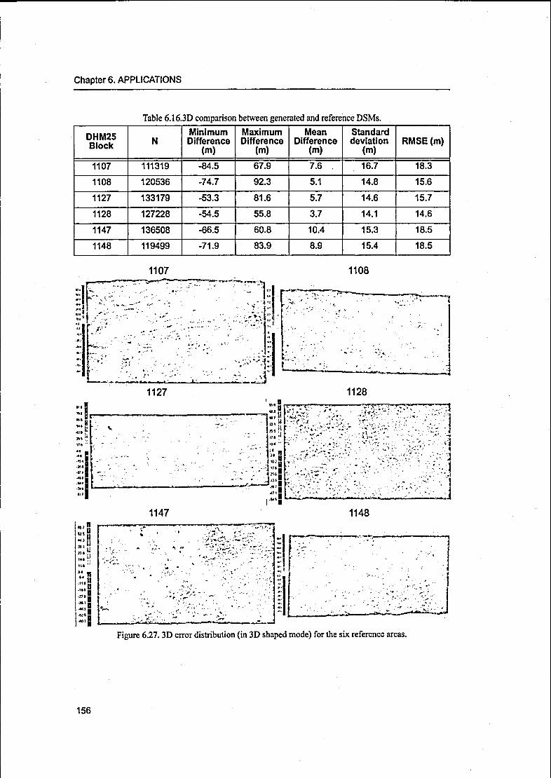
Chapter 6. APPLICATIONS
Table 6.16.3D comparison between generated and reference DSMs.
DHM25
BlockN
Minimum
Difference
(m)
Maximum
Difference
(m)
Mean
Difference
(m)
Standard
deviation
(m)RMSE (m)
1107 111319 -84.5 67.9 7.6 16.7 18.3
1108 120536 -74.7 92.3 5.1 14.8 15.6
1127 133179 -53.3 81.6 5.7 14.6 15.7
1128 127228 -54.5 55.8 3.7 14.1 14.6
1147 136508 -66.5 60.8 10.4 15.3 18.5
1148 119499 -71.9 83.9 8.9 15.4 18.5
1107 1108
Figure 6.27.3D error distribution (in 3D shaped mode) for the six reference areas.
156

Section 6.4. ASTER
1107 1127 1147
Figure 6.28.Histograms of the frequency ofthe height differences.
Figure 6.30.Slope ofthe generated DEM.
The presence of trees in areas with positive errors is also confirmed by the visual and qualitative
comparison with an orthophoto of the same area. The orthophotos were generated in 1998, with a
spatial resolution of0.5m. For this analysis the height profiles ofthe ASTER-DEM and the refer¬
ence DEM along a section have been plotted and compared. Figure 6.31 shows the location of
the section (orange line) in the orthoimage and the plot of the height profiles. It can be noticed
that the section segments where the ASTER-DEM profile is higher than the reference one corre¬
sponds to areas covered by trees in the orthoimage. In the rest of the section the fitting is quite
good.As further work, the ASTER-DEM has been imported in the commercial package Erdas Imagine8.7 (ERDASImagine, 2004) for 3D visualization. Erdas, and in particular Virtual GIS, allows the
management and visualization of geographic data, for interactive fly-through of user-defined
flight paths. For the photo-realistic visualization of the measured DEM, two products have been
used: an ASTER orthoimage and the airborne orthophotos by Swisstopo (Swisstopo, 2004), with
157

Chapter 6. APPLICATIONS
1107 1108
Figure 6.29.3D error distribution between ASTER-DEM and reference DEM and vegetation cover¬
age (dashed areas) for areas 1107,1108,1127,1128,1147 and 1148.
an accuracy of 0.5m. The ASTER othoimage has been generated with PCI Geomatica software
(PCI Geomatics, 2004), using as reference DEM the measured one and as original image a com¬
bination of the bands 1, 2 and 3N of the VNIR instrument (corresponding to the green, red and
near infrared channels). The resulting false color rectified image could be used for further land¬
scape and vegetation analysis. In this work, it was used for texture mapping. The ASTER-DEM
was imported in Erdas after the conversion in the internal file format (IMG). Afterwards, the air¬
borne orthoimages and the ASTER orthoimage have been overlapped to create two different 3D
texture model ofthe area (Figure 6.32 and Figure 6.33). In general, the fitting between the gener¬
ated DEM and the other layers (vegetation, orthoimage) is quite good, confirming the correctness
of the recovered DEM and its potential as terrain support for land cover analysis.
158

Section 6.4. ASTER
,. . ...» ., ^.
Vil' •
.
^
•"»U «#"•;„(
• 3% <.£::/•«y//
*« i.» i,' «).«•..«»
*** « XrLk-^'i
450 000
400 000
2500 5000 7500 10000
Prodi« Unght [m]
12500 15000
Figure 6.31. Analysis of a section profile in area 1128. Top: location of the section in the orthoimage;bottom: height profiles for the ASTER-DEM (green) and for the reference DEM (orange).
6.4.7 Summary and conclusions
The work described in this Section has demonstrated that using our sensor model it is possible to
orient an ASTER stereopair (channels 3N and 3B) with a sub-pixel accuracy in the check points.The images cover a variegate areas in Switzerland, with flat, hilly and mountainous terrains
(slopes in Alpine region up to 80°), lakes, rivers and urban areas. The results achieved using 8
and 12 GCPs are slightly different, demonstrating the stability of the model. The use of self-cali¬
bration was fundamental. In fact the effects due to the radial and decentering lens distortions
could reach the values of 2.0 pixels for channel 3N and 2.1 pixels for channel 3B in the imageborders. After the orientation, a 3D point cloud has been produced using the estimated parame¬
ters for the sensor internal and external orientation and about 1,800,000 points matched with
least-squares matching. The accuracy of the resulting point cloud has been evaluated comparingthe 3D distance between each point of the measured point cloud and the surface generated from
the DHM25 product by Swisstopo (l-3m accuracy). For the analyzed test sites (six blocks with
size 17.5km x 12.0km) the mean values are smaller than 1 pixel, while the RMSE and standard
deviations are slightly larger than 1 pixel. Anyway the effect of the trees, which was proved with
further analysis, was not removed. A false color orthophoto was generated from the ASTER
images and mapped onto the DEM for 3D visualization.
The results achieved in the image orientation and in the DEM accuracy are within the specifica¬tions of the absolute DEM product (5-15m for the RMSE of GCPs and 7-30m for the DEM,
Hirano et al, 2003) and in accordance with the results obtained by other authors.
In 70«//« and Cheng, 2001 an ASTER stereopair over Drum Mountains, US, was orientated
159

Chapter 6. APPLICATIONS
Figure 6.32.3D texture model with airborne orthophotos in two zoomed areas.
160

Section 6.4. ASTER
Figure 6.33.3D texture model ofthe full area (top) and two zoomed areas (bottom).
using PCI Geomatica OrthoEngine software and 8 GCPs. The residuals in 6 CPs were 15.8m,
10.5m and 7.9m. The corresponding DEM was generated and compared with an USGS 7.5-
Minute DEM (30m grid spacing), with a 7.5m RMS error. The elevation difference had a mini¬
mum value of-109m, a maximum value of 155m, a mean value of 1.9m and a standard deviation
of 11.5m with an 85% level of coincidence.
In Hirano et al, 2003 four ASTER stereoscenes located in different mountainous areas have
been used for DEM generation with R-WEL DMS software, using from 5 to 12 GCPs. The
RMSE in height in the CPs was between 7.3m and 26.3m.

Chapter 6. APPLICATIONS
6.5 MISR
Together with ASTER, the Multi-Angle SpectroRadiometer (MISR) is a part of the Earth
Observing System (EOS) of NASA. The work on MISR scenes has been developed during the
EU Cloudmap2 project (Proposal No EVK2-2000-00547).
6.5.1 Sensor description
The MISR instrument consists of nine pushbroom cameras. One camera points toward the nadir
(designated An), one bank of four cameras points in the forward direction (designated Af, Bf, Cf,and Df in order of increasing off-nadir angle), and one bank of four cameras points in the after¬
ward direction (using the same convention but designated Aa, Ba, Ca, and Da). Images are
acquired with nominal viewing angles of 0°, 26.1°, 45.6°, 60.0° and 70.5 for An, Af/Aa, Bf/
Ba, Cf/Ca, and Df/Da, respectively (Figure 6.34). Each camera uses four CCD line anays in a
single focal plane for the acquisition in four different spectral channels with special filters. The
line arrays consist of 1504 detectors plus 8 light-shielded detectors per array, each with size
21pm x 18p.m.
Figure 6.34. Multiview and multispectral acquisition ofMISR sensor. For each ofthe nine direc¬
tions, four CCD lines acquire strips in RGB and NIR channels (MISR, 2004).
The spectral band shapes are nominally gaussian and centered at 446, 558, 672, and 866 nm.
The zonal overlap swath width of the MISR imaging data (that is, the swath seen in common byall nine cameras) is 360km, which provides global multi-angle coverage of the entire Earth in 9
days at the Equator and 2 days near the Poles. The across-track IFOV and sample spacing ofeach
pixel is 275m for all of the off-nadir cameras and 250m for the nadir camera. The along-trackIFOV depends on the viewing angle, ranging from 214m in the nadir to 707m at the most oblique
angle. Sample spacing in the along-track direction is 275m in all cameras.
MISR is capable of taking image data in two different spatial resolution modes. In Local Mode
(LM), selected targets 300km long are observed at the maximum resolution of 275 meters (pixelto pixel) in all cameras (250 meters across-track for the nadir camera). However, the data trans-
162

Section 6.5. MISR
mission rate would be excessive if the instrument worked continuously at this maximum resolu¬
tion. Therefore, away from these selected targets (there will typically be only 6 ofthese each day)the instrument operates in what is termed Global Mode (GM), where Earth is observed continu¬
ously at lower resolutions. This is achieved by averaging the adjacent samples in both the across-
track and along-track directions on the ground. This averaging can be either 4 x 4, 1 x 4, or 2 x 2
pixels, and can be individually selected for each camera and spectral band (MISR, 2004). For our
purposes, GM is used.
Different operational data products are available from MISR. They are described in (Lewicki et
al, 1999) and represented in the processing chain in Figure 6.35. In this tests MISR level 1B1
Radiometric Product is used. It contains the data numbers (DNs) radiometrically-scaled to radi¬
ances. Two types of processing are included in this product. Firstly, the Radiance Scaling opera¬
tion converts the camera's digital output to a measure of energy incident on the front opticalsurface. The measurement is expressed in units called radiance (energy per unit area, wavelength,and solid angle) as defined by the an international scale. Secondly, Radiance Conditioning modi¬
fies the radiances to remove instrument-dependent effects. Specifically, image sharpening is pro¬
vided and focal-plane scattering is removed. Additionally, all radiances are adjusted to remove
slight spectral sensitivity differences among the 1504 detector elements ofeach spectral band and
each camera. This product is not geometrically corrected and therefore it can be georeferencedwith a rigorous sensor model.
Level 2TC
Level 1A Level 1B1 Level 1B2
Reformattingand annota¬
tion
—
Radiance
scaling and
conditioning-
Geometric
rectification
and registra¬tion
Top-of-atmo-sphere cloud
retrievals
Aerosol/
surface
retrievals
Level 3
Level 2AS
Figure 6.35.MISR operational products (Bothwell et al, 2002).
6.5.2 Data description
The levellBl strip conesponding to path 195 and orbit 8826, acquired on 15th August 2001, was
downloaded for free from the NASA Langley Research Center (LARC, Nasa Langley, 2004).
Among all the available strips in the NASA archive, this one was chosen because it covers central
Europe and no clouds are present in this segment. The strips acquired by each camera were con¬
tained in separate files (called granules) in HDF format. From the nine viewing directions, the
An, Afand Ab lenses (central ones) were used for this work. Each file contained the radiometric
values for blue, green, red and near infrared channels in a matrix form.
A segment of 4804 lines over central Europe was cut in each of three red-channel strips and
transformed in TIFF format in IDL environment. The resulting images, with dimensions 1504 x
4808 pixels, are represented in Figure 6.36. The acquisition time difference between An and Af
and between An and Aa is about 45sec.
163

Chapter 6. APPLICATIONS
414km 376km^
414km< 4 *
Figure 6.36. MISR scenes cut from path 195, orbit 8826. Aa (left), An (center), Af (right).The two boxes show the area analyzed
6.5.3 PreprocessingThe ephemeris corresponding to path 195, orbit 8826 were kindly provided by LARC. They con¬
tained the position and velocity every second in ECl coordinate systems (Section B.4). The data
were transformed in ECR system and the sensor attitude was calculated, as explained in Section
5.2. The value of the focal length of each lens and the detector sizes were contained in the Cam¬
era Geometric Model (CGM) file, that can be downloaded from LARC. The scenes were trans¬
formed from 11 to 8 bit with Adobe Photoshop (Adobe Photoshop, 2004). Then, in order to
facilitate the matching, they were pre-processed with Wallis filter (Section 5.3.1).
6.5.3.1 GCPs measurement.
The identification of GCPs in the MISR scenes was quite problematic due to the low ground res¬
olution of the images (275m).At the NASA Jet Propulsion Laboratory (JPL) a MISR GCP database is available. It contains 120
individual points distributed across all latitudes, the majority of which are in the United States.
About 50 points are equally distributed across Russian, African and South American regions.
164

Section 6.5. MISR
The remaining points are located in the Australia and New Zealand region. The database con¬
struction involved two stages. First is the acquisition and production of terrain-corrected Landsat
Thematic Mapper (TM) scenes over the desired ground locations. The second is the extraction of
image chips from the TM imagery and update of the Global Change Program Office (GCPO)database. Once the Landsat TM scene is selected, the terrain-conected imagery is then used as
the input to a ray-casting simulation software. The software replicates MISR viewing geometry,
producing nine images (corresponding to nine MISR cameras) which are then used for the
extraction of smaller image chips. This warping of TM imagery is necessary in order to obtain
image chips with the best possible chances to be identified in the conesponding MISR imagery(Jovanovic et al, 2002). A single MISR ground control point is a collection of nine geolocated
image patches of a well-defined and easily identifiable ground feature. The corresponding geo¬
detic coordinates define the location of a particular ground feature. The accuracy of associated
ground coordinates is expected to be 30m.
As not a single of the 120 GCPs was in path 195, we had to follow other methods.
At first we compared the images and the cartographic maps (1:25,000 or 1:50,000) of the corre¬
sponding areas in order to recognize some well-defined features, like nvers, see costs and lake
borders (Figure 6.37), but this method was very time consuming and not very accurate.
Figure 6 37. Examples of points searching along natural features (nvers, lakes, see costs) in MISR
scenes.
The main problem was the identification of the features themselves in the images. For this reason
we searched for points using other images of the same area with higher resolution, following the
strategy adopted at JPL. Requirements for the new images were a ground resolution smaller than
50m and low costs. The Landsat 7 orthoproduct available in the Web for free (ESDI, 2004) was
165

Chapter 6. APPLICATIONS
suitable for our tasks. The Landsat Project is a joint initiative of the U.S. Geological Survey
(USGS) and NASA to gather Earth resource data using a series of satellites. NASA was respon¬
sible for developing and launching the spacecraft, while the USGS was responsible for flight
operations, maintenance and management of all ground data reception, processing, archiving,product generation and distribution. The Landsat Program is the longest running enterprise for
acquisition of imagery of the Earth from space. The first Landsat satellite was launched in 1972;the most recent, Landsat 7, was launched on 15th April 1999. The instruments on the Landsat sat¬
ellites have acquired millions of images, which are archived in the United States and at Landsat
receiving stations around the world and represent a unique resource for global change research
and applications in agriculture, geology, forestry, regional planning, education and national secu¬
rity (Landsat, 2004). Today Landsat 4 (launched in 1982), Landsat 5 (launched in 1984) and
Landsat 7 (launched in 1999) are operational.The product used in this work consists of orthoim¬
ages from Enhanced Thematic Mapper Plus (ETM+) carried on board of Landsat 7 (for details
see Table 6.17). This product is georectified, with planimetric coordinates in both geographic((p,À) and UTM systems (EJV). The ETM+ is a multispectral scanning radiometer that providesimage data from eight spectral bands. The spatial resolution is 30m for the visible and near-infra¬
red (bands 1-5 and 7). Resolution for the panchromatic (band 8) is 15m, and the thermal infrared
(band 6) is 60m (Table 6.18). The approximate scene size is 170km x 183km. Eight scenes from
paths 195 and 196 covering our area of interest were downloaded and pre-processed with radio¬
metric equalization and contrast enhancement, using Wallis filter. Then 3 level pyramid images
(reduce factor of 2) were generated, so that the lowest level resolution (240m) was in the same
range of the MISR scenes resolution (275m).Common points were identified in Landsat 3rd level pyramid images and in Aa, An and AfMISR
images and matched with template multi-photo least-squares matching (Baltsavias, 1991). The
coordinates of the points of interest in Landsat images were transformed from the 3rd level to the
original one and the corresponding geographic coordinates (9, X) were read in the Landsat origi¬nal orthoimages in PCI environment (PCI Geomatics, 2004). Once the planimetric coordinates
were known, the corresponding height was read in 1:25,000 and 1:50,000 scale topographic
maps of the areas of interest. Then the ground coordinates of the matched points were trans¬
formed into the ECR system (Section B.5). A sufficient number of points were measured in two
distinct areas in the scenes: the upper part (North of Germany) and the lower part (South of
France), as indicated in Figure 6.36. In each of these areas 6 points have been measured. In addi¬
tion, 20 tie points (10 for each area) have been identified with least-squares matching in the
image space. The accuracy of associated ground coordinates was about 30m.
Table6.17.CharacteristicsofLandsat-7. Table 6.18. Specification of ETM+ instrument on
Landsat-7.
Band Spectral resolution
(urn)Resolution
(m)
1 0.45-0.515 30
2 0.525 - 0.605 30
3 0.63 - 0.690 30
4 0.75 - 0.90 30
5 1.55-1.75 30
6 10.40-12.5 60
7 2.09-2.35 30
pan 0.52 - 0.90 15
Launch date 15th April 1999
Height 705 km
Repeat cycle 16 days
Swath Width 185 km
Inclination Polar (98.2°)
Orbit Sun-synchronous
166

Section 6.5. MISR
6.5.4 Image orientation
The sensor model was separately applied on the two regions where the object points were mea¬
sured. For each region the 6 object points were all used as GCPs and the additional points wereused as TPs. Unfortunately we could not use any point for final check (CPs).The position and the attitude derived by the ancillary data were used for the direct georeferenc¬
ing. From the Camera Calibration File (Version 7), only the focal length and the pixel size could
be extracted and used. The other parameters were referring to specific systems used at JPL for
the geolocation of the MISR images and could not be converted in the systems adopted in our
model. As a consequence, the influence of the systematic errors due to the distortions ofthe opti¬cal instruments (Section 2.4.1 and Section 2.4.2) could not be taken into account a-priori and the
RMSE for the GCPs were larger than 1 pixel.Therefore the indirect georeferencing model was used to improve the internal and external orien¬
tation. According to the tests performed on ASTER, which is carried on the same platform of
MISR, the sensor external orientation was modeled with quadratic functions and three segmentswere used for the PPM. The a priori standard deviation of the GCPs was 50m. The first tests
without self-calibration were not satisfying, both in the internal (sigma naught, sigma ofTPs) and
external accuracy (RMSE of GCPs). The presence of systematic errors that were not compen¬
sated in the external orientation modelling was evident. For this reason the self-calibration was
necessary. As initial values, the additional parameters were set equal to zero. Due to the small
number of available GCPs, the self-calibrating adjustment was run fixing the external orientation
parameters to the values estimated in the previous adjustment without self-calibration. In order to
determine the APs that could be estimated, different tests were carried out varying the fixed and
free parameters. The significancy of the parameters was analyzed through their mean values,standard deviations and correlations with the other unknown parameters (Section 4.7). Due to the
low number of available object points, only the internal accuracy of the bundle adjustment could
be evaluated. The standard deviation of the TPs was 150.6m inX, 160.2m in yand 210.6m in Z
in the French site and 250.3m inX, 201.5m in Y, and 198.6m in Z for the German site. The values
refer to X, Yand Z in the ECR system. In both cases, the sigma naught a posteriori was 2p.m. For
the GCPs, the residuals had maximum values in the order of half pixel.Concerning the APs, significant values have been obtained for the principal point displacement
(Axc and Ayc), with similar values in the French and German datasets. The values for Axc were
around 1 pixel for the forward viewing lens and -1 pixel for the nadir and backward viewinglenses. The values ofAvc were slightly less than one pixel for all lenses.
6.5.5 Summary and conclusions
The MISR sensor continuously acquires systematic, global, multiangle and multispectral imag¬
ery in order to improve studies of the ecology and climate of the Earth. Within the EU-projectCloudmap2 we oriented three scenes over Europe (processing level 1B1) using our sensor model.
For this dataset the Camera Geometric Model (CGM) file was available, together with the sensor
position and velocity measured with the Tracking and Data Relay Satellite System (TDRSS). The
accuracy of the position observations was about 50m. The specific calibration datasets contained
in the CGM were estimated through an in-flight calibration, as described in Jovanovic et al,
2002.
In our case the direct georeferencing algorithm did not give satisfying results, because the lens
distortions and CCD line rotations in the focal planes were not taken into account. In fact the
camera calibration parameters contained in the CGM referred to specific coordinated systemsused at JPL and the conversion to the reference system used in our model was not possible.Among the parameters contained in the CGM, only the focal length and the pixel size values
167

Chapter 6. APPLICATIONS
were used. Without the other camera calibration parameters (and therefore assuming that no dis¬
tortions in the optical systems occur), the RMSE in the GCPs were larger than one pixel.On the other hand, using our indirect georeferencing model with 6 GCPs, the standard deviations
of the tie points and the RMSE ofthe GCPs were smaller than one pixel. These results are prom¬
ising, but further work is required for the measurement ofa larger number ofpoints to be used for
checking. The accuracy of the point measurement should be improved. In fact, even if the accu¬
racy of the ground coordinates was quite good (about 30m), the identification of the points in the
images was quite difficult.
In general, although the lack of good object points limited the tests, this work was useful to getfamiliar with low resolution images and the difficulties in their processing (above all the object
points identification) and to explore the benefits given by the combination of different resolu¬
tions images (in this case, Landsat and MISR).We have not found any publication about the accuracy that can be achieved with the combination
ofthe MISR multi-view images for the 3D coordinate estimation.
168

Section 6.6. EROS-A1
6.6 EROS-A1
The work on EROS-Al imagery was possible thanks to the collaboration with the Department of
Georesources and Land (DIGET) at the Politecnico of Turin, Italy. Even if the results achieved in
the tests are not so accurate as those obtained with the other sensors, we want to include this
work because EROS-Al has asynchronous acquisition mode and today few rigorous models
have been successfully applied for its imagery orientation (Crespi et al, 2003, Baiocchi et al,
2004, Toutin, 2004).The EROS (Earth Resources Observation System) program conducted by ImageSat International
(ISI) intends to operate a constellation of eight commercial imaging satellites in LEO (Low Earth
Orbit). The first satellite, EROS-Al, was successfully launched from the Russian START-1 pay-
load on the 5th December 2000 and is presently (April 2005) successfully operating. The second
satellite, EROS-B1, was planned to be launched in 2004 (Bar-Lev et al, 2001, Chien and Teo,
2002). The main characteristics of EROS-Al and EROS-B1 satellites are summarized in Table
6.19.
Table 6.19.Main operational parameters of EROS-Al and EROS-B1 satellites (Bar-Lev et al, 2001).
Parameter EROS-A1 EROS-B1
Weight 250kg 350kg
Dimensions (Launch) DIAM1210*2235mm DIAM 1210*2255mm
Orbit altitude 480km 600km
Lifetime over 6 years over 10 years
Imaging sensor CCD line, >7000pixels CCD TDI, 32 stages,>15000pixels
Panchromatic Imaging
GSD at Nadir
Swath
Sampling Depth
1.8m
12km
11 bits
0.87m (@600km)
13km
10bits
Multispectral Imaging
GSD at Nadir
Swath
None 4bands
3.5m
13km
Video Transmission Rate 70Mbit/sec 280Mbit/sec
6.6.1 Sensor description
EROS-Al flies along a sun-synchronous near polar orbit at a height of 480km. The NA30 cam¬
era on EROS-Al is a high-resolution pushbroom sensor with 4 CCD anays resulting in 7490
CCD elements; the scanning mode is asynchronous, that is, the satellite ground speed is faster
than its rate of imaging, as described in Section 2.5.2.2. In Standard Mode EROS-Al producespanchromatic images in the band of 500nm - 900nm wavelength at 1.8m resolution, while the
B1-B5 satellites will provide both panchromatic and multispectral imagery with better than lm
resolution. ISI provides 3 different levels of images: 0A (raw scene), 1A (radiometrically cor¬
rected scene) and IB (radiometrically and geometrically corrected scene). For our purposes, level
1A was chosen, because it preserves the original geometry ofthe acquisition.
169
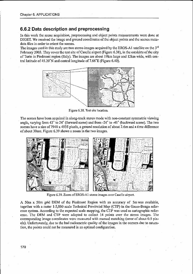
Chapter 6. APPLICATIONS
6.6.2 Data description and preprocessingIn this work the scene acquisition, preprocessing and object points measurements were done at
DIGET. We received the image and ground coordinates of the object points and the scenes meta¬
data files in order to orient the scenes.
The images used in this study are two stereo images acquired by the EROS-Al satellite on the 3rd
February 2003. They cover the test site of Caselle airport (Figure 6.38), in the outskirts ofthe cityof Turin in Piedmont region (Italy). The images are about 19km large and 12km wide, with cen¬
tral latitude of45.20°N and central longitude of 7.66°E (Figure 6.40).
Figure 6.38. Test site location.
The scenes have been acquired in along-track stereo mode with non-constant symmetric viewing
angle, varying from 43° to 24° (forward scene) and from -24° to -41° (backward scene). The two
scenes have a size of 7940 x 4935 pixels, a ground resolution of about 2.6m and a time difference
of about 30sec. Figure 6.39 shows a zoom in the two images.
Figure 6.39. Zoom ofEROS-Al stereo images over Caselle airport.
A 50m x 50m grid DEM of the Piedmont Region with an accuracy of 5m was available,
together with a raster 1:5,000 scale Technical Provincial Map (CTP) in the Gauss-Boaga refer¬
ence system. According to the expected scale mapping, the CTP was used as cartographic refer¬
ence. The DEM and CTP were adopted to collect 14 points over the stereo images. The
corresponding image coordinates were measured with manual matching (error of about 0.5 pix¬
els). Unfortunately, due to the bad radiometric quality of the images in the corners due to satura¬
tion, the points could not be measured in an optimal configuration.
170
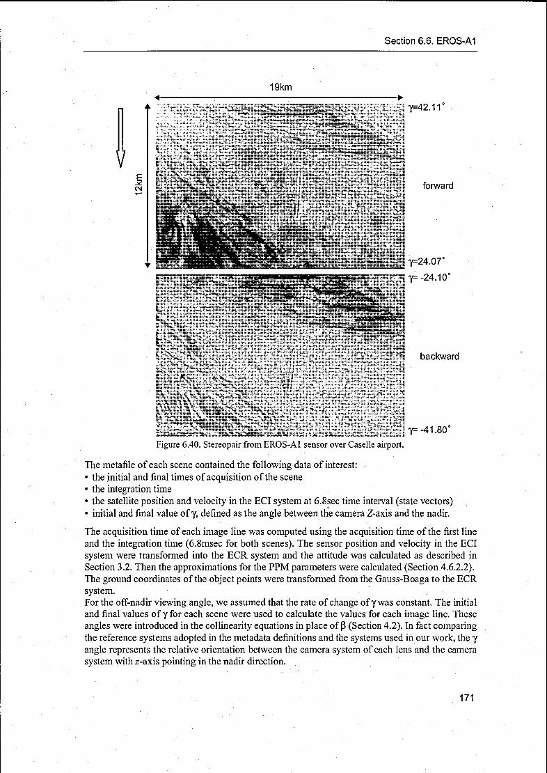
Section 6.6. EROS-A1
19km
4
Figure 6.40. Stereopair from EROS-Al sensor over Caselle airport.
The metafile of each scene contained the following data of interest:
• the initial and final times of acquisition of the scene
• the integration time• the satellite position and velocity in the ECl system at 6.8sec time interval (state vectors)• initial and final value of y, defined as the angle between the camera Z-axis and the nadir.
The acquisition time of each image line was computed using the acquisition time of the first line
and the integration time (6.8msec for both scenes). The sensor position and velocity in the ECl
system were transformed into the ECR system and the attitude was calculated as described in
Section 3.2. Then the approximations for the PPM parameters were calculated (Section 4.6.2.2).The ground coordinates of the object points were transformed from the Gauss-Boaga to the ECR
system.For the off-nadir viewing angle, we assumed that the rate of change ofy was constant. The initial
and final values of y for each scene were used to calculate the values for each image line. These
angles were introduced in the collinearity equations in place of ß (Section 4.2). In fact comparingthe reference systems adopted in the metadata definitions and the systems used in our work, the y
angle represents the relative orientation between the camera system of each lens and the camera
system with z-axis pointing in the nadir direction.
171

Chapter 6. APPLICATIONS
Points distribution
5000
4500
4000
3500
3000
2500
2000
1500
1000(
500
1 i I I i 1 1
- i .
•109
-
•103
•112'
110
•101
-
104
1 ' •1».,03-
'•111•114
- '
10?-
- •Î15•10S
j
Ï05• ' -
i I i ' '
107
1000 2000 3000 4000
Column
5000 6000 7000
Figure 6.41.Distribution of 13 object points in the image system.
The indirect georeferencing model, that was originally designed for fixed relative orientation
angles (a, ß, y), was adapted in order to read the relative orientation angles with linear variations.
6.6.3 Image orientation
The georeferencing was performed in the ECR system. A group of available points were used as
GCPs and the remaining as control (CPs). As the total number of object points was 14, 8 pointswere used as GCPs and 6 points as CPs. The a-priori standard deviation of the GCPs was lm.
Different tests were performed in order to decide the distribution of GCPs, the number of trajec¬
tory segments and the polynomial degree for the PPM and the additional parameters in the self-
calibration.
Each test consisted of a two-step processing. At first the external orientation only was estimated,then it was fixed to the estimated values and the adjustment was repeated with self-calibration,
varying the free APs. About the external orientation modelling, there was not a considerable dif¬
ference between using 2 or 4 segments for the piecewise functions, but the results were much
worse ifthe polynomial degree was decreased from 2 to 1. Therefore the external orientation was
modelled with 2 segments of 2nd order polynomials.The conelation between the APs, the external orientation parameters and the ground coordinates
of the CPs were analyzed in order to decide the APs that could be estimated. Finally the internal
orientation parameter that mostly affected the results was the scale in y direction, that is sy Using8 GCPs and 6 CPs, the internal orientation accuracy (sigma of CPs) achieved was 3.3m in X,2.6m in Y and 5.7m in Z (1.3, 1.0 and 2.2 pixels). Sigma naught a posteriori was 0.024mm (1.3pixels). The RMSE of CPs were 4.8m inX, 2.7m in Fand 5.9 in Z, corresponding to 1.8, 1.0 and
2.3 pixels. The differences between the RMSE and sigma values of the ground coordinates of the
CPs can be due to the wrong weight assignment fo the image and ground coordinates of the
GCPs and CPs or to the presence of additional errors that have not been compensated in the
model. Even if the accuracy achieved is larger than 1 pixel, the results are promising.The difficulties encountered with EROS imagery mostly related due to the understanding of all
the attitude parameters contained in the metadata files and in the modelling of the asynchronousacquisition. For example, we took the values for the off-nadir angles y reported in the metadata
172

Section 6.6. EROS-A1
file as the relative orientation angle ß for our system. Although this assumption was justified bythe reference systems description in the users' EROS documentation, it may not be completelycorrect. Another aspect to take into account is that, due to the lack of detailed information on the
acquisition geometry, we assumed that the rate of change ofy was constant. This may also intro¬
duce additional errors. Concerning the bundle adjustment, the non-optimal distribution of the
GCPs influenced its performance.
6.6.4 Summary and conclusions
Thanks to the collaboration with the Department of Georesources and Land of the Politecnico of
Turin (DIGET), who provided the dataset, we oriented a stereo pair acquired by EROS-Al with
our sensor model. Due to the lack of information on the sensor internal and external orientation,the self-calibrating bundle adjustment contained in the indirect georeferencing model was used,with 6 GCPs and 8 CPs. The accuracy achieved in the CPs was 3.3m inX, 2.6m in 7 and 5.7m in
Z (1.3, 1.0 and 2.2 pixels) for the standard deviation and 4.8m in X, 2.7m in 7and 5.9 in Z (1.8,1.0 and 2.3 pixels) for the RMSE. Sigma naught a posteriori was 0.024mm (1.3 pixels).We have also concluded that if more knowledge on the sensor geometry will be available, then
more correct parameters for the viewing angles could be calculated and the model performance
improved.The asynchronous acquisition of EROS-Al causes some difficulties in the rigorous modelling of
the images. Today few rigorous models have been applied for the georeferencing of EROS-Al
imagery and can be used for a validation ofour results.
The SISAR rigorous model, developed at the University ofRome, has been used for the orthorec¬
tification of 4 EROS-Al images with a ground resolution of 1.8m and acquired with different y
angle (Baiocchi et al, 2004). Using a minimum of 9 GCPs, the RMSE achieved in at least 40
CPs were 3.7m in East and 2.1m in North. Using the rigorous model and the RPC model in PCI
Geomatica similar results were obtained. In Toutin et al, 2002 the RMSE obtained with the rig¬orous model in PCI Geomatica and 10 GCPs was 3.9m in East and 3.5m in North (14 CPs,
ground resolution of 2m).
Again with this commercial software, an EROS-Al stereo pair acquired over Québec, Canada,
was oriented using 18 GCPs. The RMSE in the 112 CPs were 4.2m in East, 4.2m in North and
5.9m in height (ground resolution of 1.8m).From this analysis it can be concluded that the results achieved with our approach are close to
those obtained with other rigorous models available in commercial software. Anyway, we think
that the results can be improved if a deeper knowledge on the sensor geometry is available.
173

Chapter 6. APPLICATIONS
174

7
CONCLUSIONS AND OUTLOOK
7.1 CONCLUSIONS
In this thesis the geometric modelling ofpushbroom sensors has been investigated and the rigor¬ous model implemented for their orientation has been presented. The imagery acquired by this
kind of sensors has very high potential for photogrammetric mapping at different scales from air¬
borne and satellite platforms and its orientation is a fundamental step in the processing chain for
the generation of orthoimages and Digital Elevation Models (DEMs).As seen in the Introduction, today various models based on different approaches have been
developed, but few of them are rigorous and can be used for a wide class of pushbroom sensors.
On the other hand it has been demonstrated that the sensor model presented in this thesis can be
applied for the orientation of linear array scanners with different camera designs.In general a rigorous sensor model aims to describe the relationship between image and groundcoordinates, according to the physical properties of the image acquisition. In order to developsuch a model, the analysis of different aspects of pushbroom sensors (optical system, linear
arrays geometry, acquisition mode) and their imagery (resolutions, processing levels) were inves¬
tigated in Chapter 2.
The proposed model includes two different orientation approaches, described in Chapters 3 and
4. In the direct georeferencing model the ground coordinates of the homologous points measuredin the images are estimated through a forward intersection, using as external orientation the data
provided by geopositioning systems carried on board (GPS, INS, star trackers) or the trajectorycalculated by mathematical formulas describing the sensor trajectory (only for satellite-based
sensors). This approach does not require any ground control points, except for final checking,and does not estimate any additional parameters for the correction of the interior and exterior ori¬
entation. For this reason, the accuracy of this method depends on the accuracy ofthe external and
175

Chapter 7. CONCLUSIONS AND OUTLOOK
internal orientation data. Theoretically the use ofGPS and INS is very powerful, because it could
allow point positioning without ground information. The GPS and INS data must be transformed
into the camera reference system with the knowledge of the systems displacements and misalign¬ments. Moreover the measurements provided by these instruments may contain systematic errors
that must be modelled and compensated. Therefore in practice up to day the positioning systemscan only greatly reduce, but not completely eliminate the need for ground control. This is more
valid in case of airborne pushbroom sensors, because of the vibrations and the instability of the
platform's trajectory. Since the need for ground control points cannot be eliminated with the use
of GPS, the integration of positioning systems, that is the integration of GPS and INS observa¬
tions, into a bundle adjustment became a subject of research in this field.
The alternative orientation method, based on indirect georeferencing, is used if the sensor exter¬
nal and internal orientation is not available or not enough accurate for high-precision photogram¬metric mapping. This approach is a self-calibrating bundle adjustment, but modified according to
the pushbroom sensors' characteristics. The sensor position and attitude are modelled with 2nd
order piecewise polynomial functions (PPM) depending on time. Constraints on the segment bor¬
ders assure the continuity of the functions, together with their first and second derivatives. Using
pseudo-observations on the PPM parameters, the polynomial degree can be reduced to one (lin¬ear functions) or even to zero (constant functions). If GPS and INS are available, they are inte¬
grated in the PPM. In this case the constant terms are used to correct the data from the
misalignments between the GPS/INS systems and the camera frame, while the 1st and 2nd order
terms describe other systematic errors contained in the observations. For the self-calibration,additional parameters (APs) are used to model the lens internal parameters and distortions and
the linear arrays displacements in the focal plane.The parameters modelling the internal and external orientation, together with the ground coordi¬
nates ofthe tie points, are estimated through a least-squares bundle adjustment using well distrib¬
uted ground control points. The use ofpseudo-observations allows the user to run the adjustment
fixing any unknown parameters to certain values. This option is very useful not only for the
external orientation modelling, but also for the analysis of the single self-calibration parameters'influence. The weights for the observations and pseudo-observations are determined according to
the measurement accuracy.
A blunder detection procedure is integrated for the automatic detection of wrong image coordi¬
nate measurements. The false measurements removal is manual.
The adjustment results are analyzed in terms of internal and external accuracy. The APs to be
estimated are chosen according to their conelations with the other unknown parameters (groundcoordinates of tie points and PPM parameters).
The model has been developed under Unix environment in C language. The software reads files
with predefined formats and extensions, containing information on the camera geometric charac¬
teristics, the acquisition time of each image line, the external orientation data, any calibration
parameters and the image and ground coordinates of the tie points (Appendix C). The object ref¬
erence systems accepted are the fixed cartesian geocentric (ECR), the geographic system and any
local tangent systems. The algorithms for the coordinates transformation from one system to the
other have also been included.
Working with satellite imagery, the ECR system is used. In case of airborne imagery, the local
tangent systems are adopted as reference frame.
One fundamental requirement for this model was the flexibility, that is, the possibility to be used
for the orientation of a wide class of pushbroom sensors. In order to demonstrate it, the model
was tested on different pushbroom imagery. The results obtained from an airborne dataset, pre-
176

Section 7.2. OUTLOOK
sented in Poli, 2002b, demonstrated the need of modelling the systematic errors contained in the
GPS and INS measurements through a bundle adjustment.On the other hand, the results obtained from satellite imagery were reported in Chapter 6. The
sensors used in our tests were MOMS-P2, SPOT-5/HRS, ASTER, MISR and EROS-Al. It can be
noted that these sensors have different characteristics (single-lens and multi-lens optical systems,various number of linear arrays, synchronous and asynchronous acquisition modes), covering a
wide range of possible acquisition geometries.For each dataset both the direct and indirect models have been used and in all cases the direct
georeferencing was not accurate enough for high accurate mapping. The indirect model has been
applied with different ground control points distributions (when possible), varying the PPM con¬
figurations (number of segments, polynomials degree) and with and without self-calibration.
Excluding EROS-Al, all the imagery has been oriented with sub-pixels accuracy in the check
points using a minimum number of 6 ground control points. In case of EROS-Al, an accuracy in
the range of 1 to 2 pixels has been achieved, due the lack of information on the geometry of the
sensor asynchronous acquisition. The self-calibration is usually recommended.
New cameras can be easily integrated in the model. In fact the required sensor information (num¬ber of linear arrays, number of lenses, focal length, number of detector elements in each line,
viewing angles) are accessible in literature as well as in the web. If no information on the sensor
internal orientation is available, the model supposes that the CCD lines are parallel to each other
in the focal plane and perpendicular to the flight direction and estimates any systematic enor
through the self-calibration. Concerning the external orientation, in case of spaceborne sensors
the satellite's position and velocity vectors, usually contained in the ephemeris, are required in
order to compute the initial approximations for the PPM parameters. If this information is not
available, the orbit's Keplerian elements can be used to estimate the nominal trajectory. For push¬broom scanners carried on airplane or helicopter the GPS and INS measurements are indispens¬able, due to the unpredictability of the trajectory.In conclusion, in this thesis the rigorous sensor model for pushbroom sensors has been presentedand its flexibility demonstrated through a variety of tests.
7.2 OUTLOOK
Further investigations could be carried out in order to improve the sensor model's potentials.For the satellite sensors the calculation of the platform position based on the Keplerian elements
can be improved by taking into account the orbit oscillations. In fact the assumptions of the used
theory is that the satellite movement is caused by the gravity force only. In practise other forces
take part and cause secondary effects that can be modeled by combination of sinusoidal and poly¬nomial functions. The size of these effects must be investigated.Future work includes also a further study on the determinability ofthe additional parameters used
in the self-calibration. With the cunent software the user can analyze the correlation between the
parameters and choose which parameters must be fixed. This operation could be automated bymeans of determinability and significance tests at each iteration. The blunder detection and
removal could also be improved and made automatic.
Even ifthe model flexibility has been demonstrated, more tests are suggested in order to take into
account other acquisition geometries of pushbroom sensors. For example the sensors with
across-track stereo capability could be included in the model. In this case the number of trajecto¬ries to be modelled is two instead of one, as in the along-track stereo sensors, but constraints
between consecutive trajectories can be imposed according to the orbit's geometry (inclination,period).
177

Chapter 7. CONCLUSIONS AND OUTLOOK
Another possible development is the implementation of a user-friendly interface. This interface
should contain the following functions: selection of the input files containing the sensor charac¬
teristics, the calibration data and the external orientation data, definition of reference system for
object points and external orientation, choice of reference systems for bundle adjustment, intro¬
duction of initial values for self-calibration parameters, selection of external and internal orienta¬
tion parameters to be fixed, choice of number of iterations.
Now these information are introduced through a UNIX shell or by means of input files contain¬
ing the information themselves. A difficulty often encountered with satellite sensors is that the
metadata files containing information about the scenes (acquisition time, ephemeris, internal
geometry, etc.) have a different format for each sensor. In order to render the model more user-
friendly, the automatic extraction of the required information from the metadata files could be
implemented.
178

Appendix A
ACRONYMS
A.1 Sensors and Missions
AATSR: Advanced Along Track Scanning Radiometer
ADEOS: Advanced Earth Observation Satellite
ADS: Airborne Digital Sensor
AirMISR: Airborne Multi-Angle Imaging SpectroRadiometer
ALOS: Advanced Land Observation Satellite
ASTER: Advanced Spaceborne Thermal Emission and Radiation Radiometer
BIRD: Bispectral Infrared Detector
CASI: Compact Airborne Spectrographic Imager
CERES: Clouds and the Earth's Radiant Energy System
DPA: Digitales Photogrammetrisches Auswertesystem
EOS: Earth Observing System
EROS: Earth Resources Observation Satellite
ETM+: Enhanced Thermic Mapper Plus
GLI: Global Imager
HRG: High Resolution Geometry
HRSC: High Resolution Stereo Camera
HRV: High Resolution Visible
1RS: Indian Remote Sensing Satellite
MEOSS: Monocular Electro-Optical Stereo Scanner
MISR: Multi-Angle Imaging SpectroRadiometer
MODIS: Moderate-Resolution Imaging Spectroradiometer
MOMS-02: Modular Optoelectronic Multispectral Scanner
MOPITT: Measurements Of Pollution In The Troposphere
179

Appendix A. ACRONYMS
PRISM: Panchromatic Remote-sensing Instrument for Stereo Mapping
R21: Resource 21
SPOT: Système Pour l'Observation de la Terre
TLS: Three-Line Scanner
WAAC: Wide-Angle Airborne Camera
WAOSS: Wide-Angle Optoelectronic Stereo Scanner
A.2 Space Agencies and Remote Sensing Organizations
CCRS: Canada Centre for Remote Sensing
CEOS: Committee on Earth Observation Satellites
CNES: Centre National d'Etudes Spatiales
DARA: Deutsche Agentur für Raumfahrtangelegenheiten
DASA: Daimler Benz AeroSpace
DLR: Deutschen Zentrum für Luft- und Raumfahrt
JAXA: Japan Aerospace Exploration AgencyNASA: National Aeronautics and Space Administration
NASDA: National Space Development Agency of Japan
USGS: United States Geological Survey
A.3 Other acronyms
CCD: Charge Coupled Device
CMOS: Complementary Metal-Oxide Semiconductor
CP: Check Point
DGPS: Differential GPS
GCP: Ground Control Point
GPS: Global Positioning System
INS: Inertial Navigation System
LSM: Least Squares Matching
MPGC: Multi-Photo Geometrically Constraint
PC: Perspective Center
RMSE: Root Mean Square Error
TP: Tie Points
180

Appendix B
REFERENCE SYSTEMS
In the following Sections the reference systems used in this thesis are summarized.
B.1 Image coordinate system
It is a 2 dimensional system describing a point position in an image. The origin is at the centre of
the left top pixel; the pixel position is defined by its row (u) and column (v). The image dimen¬
sions are called with N„ (width, number of pixels contained in a row) and Nr (height, number of
column rows).
Nn
0,0
Nr
-> columns
i
rows
Figure B.l. Image system.
B.2 Scanline system
It is a 2D system defined for each image line. It is centered in the mean pixel of the line, with ys
axis parallel to the image line and xs axis perpendicular toys axis, close to the flight direction.
181

Appendix B. REFERENCE SYSTEMS
Assuming an ideal case without lens distortions and geometric errors in the CCD line, the coordi¬
nate^ can be calculated with the transformation
y< 44> (8.1)
where py is the pixel dimension inys direction and A^, is the number of pixels in each line. The
coordinate xs is fixed equal to zero.
If the pre-flight laboratory calibration results are available, the given exact position of each CCDline in the focal plane are used as xs andys values (Figure B.2).
Nn
ys
Figure B.2. Scanline system.
The time of acquisition t, of line i can be calculated using the time of acquisition of a line of ref¬
erence (indicated by the subscript 0, usually the first line) and the integration time (Af), that is,the time required by the optical system to scan one line on the ground
h = 'o + (M«-"o)A' (B.2)
«,- and uq stand for the row numbers of line i and 0 and tg is the time of acquisition of the refer¬
ence line.
B.3 Camera system
The camera system (indicated with letter C) is a 3D system centered in the perspective center
(PC) of each lens. The axis xc and_yc are parallel to xs and_ys. The z-axis zc is upwards directed
and completes a right-hand coordinate system. The value of zc is equal to the lens focal length.
Each lens consisting the optical system has its own camera reference system (example of three-
line sensor, Figure B3).
Flight direction
//
/
M
ft I v-
JU%
Focalptane
//
/
Flight direction
Figure B.3. Camera system in case of one lens (right) and more-lens (left) optical systems.
182

Section B.4. Geocentric inertial coordinate system (ECl)
B.4 Geocentric inertial coordinate system (ECl)
The origin is in the centre of gravity of the Earth, the Z-axis points toward the North Pole, the X-
axis lies in the equatorial plane and is directed toward the vernal equinox (JR2000), the i^axis
completes a right handed orthogonal system by a plane 90° east of the Z-axis and its intersection
with the Equator.
Figure B.4. Geocentric Cartesian Inertial coordinate system.
B.5 Geocentric fixed coordinate system (ECR)
The origin is in the centre of gravity of the Earth, the Z-axis points toward the North Pole, the X-
axis is defined by the intersection of the plane defined by the prime meridian (Greenwich) and
the equatorial plane, the J^-axis completes a right handed orthogonal system by a plane 90° East
of the X-axis and its intersection with the Equator.
Greenwich A
Figure B.5. Geocentric Cartesian coordinate system.
B.6 Geographic coordinates
They are described by latitude, longitude, height (<p, X, h). The Prime Meridian and the Equatorare the reference planes used to define latitude and longitude. The geographic latitude of a pointis the angle from the equatorial plane to the vertical direction of a line normal to the reference
ellipsoid. The geographic longitude ofa point is the angle between a reference plane and a planepassing through the point, both planes being perpendicular to the equatorial plane. The geodetic
183

Appendix B. REFERENCE SYSTEMS
height at a point is the distance from the reference ellipsoid to the point in a direction normal to
the ellipsoid.
EllipsoidSurface
Equator
Pole Geodetic Height of
Point P
Semi Minor Axis
\y\ Point P
Normal to j
Ellipsoid at^rPomtPj/\
S \ Tangent to Ellipse\ at Point P
——•«<••'***"
Geodetic4
Longitude af
Point P
Geodetic
Latitude at
Point PTHVtnWOM
Figure B.6.Geodetic coordinate system (Dana, 2004).
The transformation from (cp, X, h) Xo(X, Y,Z) is
X = (N + A) cos (p cos A
Y = (N + /i)cos(psinA
Z = [AT(l-e2)-r/z]sincp(B.3)
a-b1where e2 = -—-— is the eccentricity of the Earth ellipsoid (being a and b the major and minor
a
Earth radius) and N =
1 -(sin(p)
is the radius of curvature of a point with latitude (p in the
prime vertical.
B.7 Local coordinate system
A local coordinate system is a right-hand system centered at a chosen point P with X-axis tangentto the local parallel and looking toward East, i^axis tangent to the local meridian and lookingtoward North and Z-axis upwards directed.
Calling Xp, Yp, Zp the geocentric coordinates of the origin of the ground local system (point P)and (pP and ÀP its latitude and longitude, the transformation from the geocentric to the ground
local system is (Wang, 1999, p. 152)
Rx(90-<pp)R (90-Xp)
X-Xj
Y-Yf
Z-Zn
(B.4)
where (X, Y, Z) are the coordinates in the geocentric system, (Xi, Y^, Z{) in the ground local sys¬
tem.
184
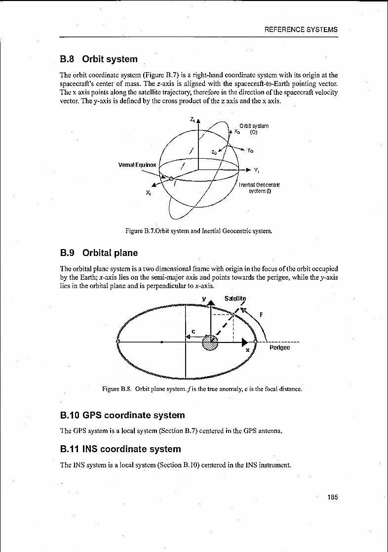
REFERENCE SYSTEMS
B.8 Orbit system
The orbit coordinate system (Figure B.7) is a right-hand coordinate system with its origin at the
spacecraft's center of mass. The z-axis is aligned with the spacecraft-to-Earth pointing vector.
The x axis points along the satellite trajectory, therefore in the direction of the spacecraft velocityvector. The y-axis is defined by the cross product of the z axis and the x axis.
Vernal Equinox
Orbit systemXo (0)
Inertial Geocentric
system (I)
Figure B.7.0rbit system and Inertial Geocentric system.
B.9 Orbital plane
The orbital plane system is a two dimensional frame with origin in the focus ofthe orbit occupiedby the Earth; jc-axis lies on the semi-major axis and points towards the perigee, while the j-axislies in the orbital plane and is perpendicular to A--axis.
SatelliteS
Figure B.8. Orbit plane system./is the true anomaly, c is the focal distance.
B.10 GPS coordinate system
The GPS system is a local system (Section B.7) centered in the GPS antenna.
B.11 INS coordinate system
The INS system is a local system (Section B.10) centered in the INS instrument.
185

Appendix B. REFERENCE SYSTEMS
186

Appendix C
SOFTWARE DESCRIPTION
The direct georeferencing software is called push_model_direct and the indirect georeferencingsoftware is called push_model_indirect. They have been developed in C language in Unix envi¬
ronment. The two programs follow the same logic for the input and output files.
In input, the programs ask a base. For semplicity, the base is usually the name ofthe sensor (forexample, misr, aster, hrs,...), but any name can be used. From the base, two files are automati¬
cally identified:
• base.data contains information about the sensor characteristics (number of lenses, number of
viewing directions, image dimension in pixels) and for each viewing direction: an integer num¬ber that identifies the viewing direction, the viewing angle in degrees, the focal length of the
corresponding lens (in mm) and the pixel size in the row and column direction (in mm). All
these data are easily accessible from the web, from literature or from the metadata files. New
sensors can be added to the model if the corresponding base.data files are available. Here is
misr.data file for MISR sensor:
9 9 /*nuitiber of lenses, number of viewing directions*/
4801 1504 /*image dimension (number of rows and columns)*/
/identifier, viewing angle, focal length, pixel size*/
1 -70.500 123.800 0.021 0.018
.018
0.018
.018
0.018
.018
.018
.018
.018
Ifthe images have different dimensions, like for ASTER, the code 99999 is used in place ofthe
image dimensions and the dimensions of each image are written at the end of the file.
2 -60 000 95.300 0.021 0
3 -45 600 73.400 0.021 0
4 -23 3186 59.025 0.021 0
5 -0 0314 58.944 0.021 0
6 23 2778 58.903 0.021 0
7 45 600 73.400 0.021 0
8 60 000 95.300 0.021 0
9 70 500 123.800 0.021 0
187

Appendix C. SOFTWARE DESCRIPTION
• base.ip contains the image coordinates of the points observed in the images. Each point can be
observed in a variable number of images. The image coordinates are given in format: name,
viewing direction number (same notation used in base.data), image coordinates (column, row)in pixels. In order to read the points automatically, the code 99999 is used to separate them.
Here is an example with 2 image points:2
l
4.
682.438000 48.438000
5 687.158000 16.763000
6 702.721000 9.298000
99999
2
4 731.625000 64.875000
5 740.982000 33.006000
6 751.608000 25.900000
99999
Then few questions are asked about the available external orientation (with or without GPS and
INS, reference system) and the calibration.
According to these answers, files with fixed suffix are found:
• base_pos.xxx and base_att.xxx: files with position and attitude data; we can have one file for
each viewing direction or one file for the aircraft or spacecraft position/attitude. According to
this format and the reference system (Geocentric, Geographic, local), the corresponding files
are read. For example, in case of one file for position and attitude in local system, the program
will search for files base.pos.loc and base.att.loc. Further questions are asked in order to distin¬
guish if the position and attitude are for each image-line or if the position and attitude are not
synchronised with the acquisition times (in this case cubic splines interpolate the data and the
value for the time of interest is calculated and additional files containing the time of acquisitionofeach image-lines are required)
• base_n.cal, where n is the line/lens number: files with calibration data, that is, position of each
pixel in the focal plane.
For the indirect georeferencing model the program also asks: the numbers of Ground Control
Points (GCPs), Tie Points (TPs) and Check Points (CPs), the maximum number of iterations, the
external and self-calibration parameters to estimate, the weights for the image observations, the
external and internal orientation approximations and the GCP coordinates, the number of seg¬
ments for the PPM and the thresholds to use to stop the adjustment.The GCPs are contained in:
• base__gcp.xxx: according to the reference system, the files that can be read are base_gcp.geocfor Geocentric system, base_gcp.geog for Geographic system, base_gcp.loc for local systems
In output, the solutions are stored files with pre-defined name.In case of direct georeferencing, we have:
• baseji.ground: file with forward intersection results (object coordinates of points in base.ip).
In case of indirect georeferencing, the output files are:
• base.eo: file with estimated external orientation parameters• base.sc: file with estimated self-calibration parameters• base.tp: file with estimated object coordinates of GCPs and TPs
• base.iter: file with statistics for each iteration
• base.sum: file with summary of input and output data and adjustment performances (sigmanaught a posteriori, sigma ofestimated parameters, RMSE of CPs).
188

BIBLIOGRAPHY
The references are listed in alphabetic order. The following abbreviations are used:
ACRS: Asian Conference of Remote SensingASPRS: American Society ofPhotogrammetry and Remote SensingEaRSeL: European Association of Remote Sensing Laboratories
IAPRS: International Archives ofPhotogrammetry and Remote SensingISPRS: International Society ofPhotogrammetry and Remote SensingPE&RS: Photogrammetric Engineering and Remote Sensing
Abrams, M., Hook, S., 2002. ASTER User HandBook. Available at http://asterweb.jpl.nasa.gov/documents/aster_user_guide_v2.pdf(last visited August 2004).
Ackermann, F., 1986. The use of camera orientation data in photogrammetry. IAPRS, Vol. 26,
Parti, pp. 93-99.
Ackermann, F., Bodechtel, J., Lanzl, F., Meissner, D., Seige, P., 1986. MOMS-02 ein multispek¬trales Stereo Bildaufnahmensystem für die zweite deutsche Spacelab Mission D2, Geo-Infor-mationssystem (GIS), 2(3), pp. 5-11.
AirMISR, 2004. http://www-misr.jpl.nasa.gov/mission/air.html (last visited June 2004)
Adobe Photoshop, 2004. http://www.adobe.com/products/photoshop/main.html (last visited
August 2004).
ALOS Project, 2004. http://alos.nasda.go.jp/main2e.html (last visited June 2004)
Ames Remote, 2004. http://www.amesremote.com (last visited March 2005)
Applanix, 2004. http://wvvw.applanix.com (last visited August 2004).
189

BIBLIOGRAPHY
ArcGIS ESRI, 2004. http://www.esri.com/software/arcgis (last visited November 2004).
ASTER, 2004. http://asterweb.jpl.nasa.gov (last visited August 2004).
Baiocchi, V., Crespi, M., De Vindictis, L., Giannone, F., 2004. A new rigorous model for the
orthorectification of synchronous and asynchronous high resolution imagery. EaRSeL, May2004. Proceedings on CDROM.
Ball Aerospace, 2004. http://www.ballaerospace.com (last visited June 2004)
Baltsavias, E. P., 1991. Multiphoto geometrically constrained matching. Ph. D. dissertation,Institute of Geodesy and Photogrammetry, ETH Zürich, Mitteilungen No. 49.
Baltsavias E. P., Stallmann D., 1992. Metric Information Extraction from SPOT Images and the
Role of Polynomial Mapping Functions. IAPRS, Vol. 29, Part B4, Washington, pp. 358 - 364.
Baltsavias E. P., Stallmann D., 1993. SPOT Stereo Matching for DTM Generation. Paper pre¬
sented at the Conference "Integrating Photogrammetric Techniques with Scene Analysis and
Machine Vision", 12. - 16. April, Orlando, USA. In Proc. of SPIE, Vol. 1944, pp. 152 -163.
Baltsavias E. P., Li H., Mason S., Stefanidis A., Sinning M., 1996: Comparison of Two Digital
Photogrammetric Systems with Emphasis on DTM Generation: Case Study Glacier Measure¬
ment. IAPRS, Vol. 31, Part B4, Vienna, pp. 104 - 109.
Baltsavias, E. P., Stallmann, D., 1996. Geometric potential ofMOMS-02/D2 data for point posi¬tioning, DTM and orthoimage. IAPRS, Vol. 31, Part B4, Vienna, pp. 110-116.
Baltsavias, E.P., 2000. Future ofphotogrammetric scanners and film scanning. GIM, Vol. 14, No.
3, pp. 36-39.
Baltsavias, E. P., Pateraki, M., Zhang, L., 2001. Radiometric and Geometric Evaluation of
IKONOS Geo Images and their use for 3D building modelling. Proceedings of ISPRS Work¬
shop "High resolution mapping from space 2001", 18-21 September, Hannover, Germany.
Proceedings on CDROM.
Bar-Lev, M., Shcherbina, L., Levin, V, 2001. EROS system- Satellite orbit and constellation
design. Proceedings of 22nd Asian Conference on Remote Sensing 2001, 5-9 September, Sin¬
gapore, Part 2, pp. 1153-1158.
Baudoin, A., Schroeder, M., Valorge, C, Bernard, M., Rudowski, V, 2004. The HRS-SAR Initia¬
tive: a scientific assessment of the High Resolution Stereoscopic instrument on board of
SPOT 5 by ISPRS Investigators. IAPRS, Vol. 35, Part Bl, Istanbul, pp. 372-378.
Beyer, H.A., 1992. Geometric and radiometric analysis of a CCD-Camera based photogrammet¬ric close-range system. PhD thesis, Institut fur Geodäsie und Photogrammetry, Nr. 51, ETH,
Zurich, May 1992.
Bayerische Vermessungsverwaltung, 2004. http://www.geodaten.bayern.de (last visited August2004).
190

BIBLIOGRAPHY
Blanc, N., 2001. CCD versus CMOS - has CCD imaging come to an end? Proceedings of Photo¬
grammetric Week 2001, Stuttgard. Proceedings on CDROM.
D.C. Brown, 1971. Close-range camera calibration. Photogrammetric Engineering. Vol.37, Nr. 8,
pp.855-866.
Bothwell, G. W, Hansen, E. G., Vargo, R. E., Miller, K. C, 2002. The Multi-angle ImagingSpectroRadiometer science data system, its products, tools and performance. IEEE Transac¬
tion on Geoscience and Remote Sensing, Vol. 40, No. 7, pp. 1467-1476.
Büyüksalih G., Jacobsen K., 2000. Geometric aspects ofMOMS-2P three-line imagery for map¬
ping applications. Annual Meeting of the Remote Sensing Society, Lancaster, UK.
CCRS Tutorial, 2004. http://www.ccrs.nrcan.gc.ca/ccrs/learn/tutorials/tutorials_e.html (last vis¬
ited August 2004).
CEOS, 2004. http://www.ceos.cnes.fr (last visited June 2004)
Chen, L., Wu, Y, 2000. Image Geometric Simulation And Orientation Modeling For Rocsat-2.
Proceedings ofACRS, Taipei, Taiwan, 4-8 December. Proceedings on CDROM.
Chen, L. C, Teo, T. A., 2002. Rigorous generation of digital orthophoto from EROS A high res¬
olution satellite images. IAPRS, Vol. 34, Part B4, Ottawa, pp. 620-625.
Chen, T., Shibasaki, R., Murai, S., 2003. Development and calibration of the airborne three-line
scanner (TLS) imaging system. PE&RS, Vol. 69, No. 1, January 2003, pp. 71-78.
Chien, L.C., Teo, T.-A., 2002. Rigorous generation ofdigital orthophotosfrom EROS 1 high res¬
olution satellite images. IAPRS, Vol. 34, Part B4, Ottawa, pp.620-625.
Choi, J., Dongarra, J. J., Ostrouchov L. S., Petitet, A. P., Walker, D. W., Whaley, R. C, 1994,The Design and Implementation of the ScaLAPACK LU, QR, and Cholesky Factorization
Routines. Department ofComputer Science, University ofTennessee, Mathematical Sciences
Section, September 1994. Available at http://www.netlib.org/utk/papers/factor/ftcover.html(last visited August 2004).
CNES, 2004. http://www.cnes.fr (last visited June 2004).
Cramer M., 1999. Direct Geocoding: is Aerial Triangulation Obsolete?. Photogrammetric Week
1999, Fritsch/Spiller (eds), Wichmann Verlag, Heidelberg, Germany, pp. 59-70, 1999.
Cramer, M., Stallmann, D., Haala, N., 2000b. Direct georeferencing using GPS/INS exterior ori¬
entations for photogrammetric applications. IAPRS, Vol. 33, Part B3, Amsterdam, pp. 198-
205.
Crespi, M., Baiocchi, V, De Vendictis, L., Lorenzon, F., Mezzapesa, M., 2003. Un modello rig¬oroso per l'ortorettificazione delle immagini del satellite EROS-Al. Proceedings of ASITA
2003 Conference, Verona, October 2003, Vol. I, pp. 849-856
191

BIBLIOGRAPHY
Crippa, B., Forlani, G., 1990. II calcolo con gli elementi finiti. Ricerche di Geodesia, Topografiae Fotogrammetria, Vol. 6., Citta'Studi ed., Milano, 1990.
Dana, P. H.„ 2004. http://www.pdana.com/PHDWWW.htm (last visited August 2004).
De Boor, C, 1912>. A practical guide to splines. Springier-Verlag ed., New York, 1978
Denore B. J., 2000. On how future low-cost remote sensing satellites could meet the information
needs of environmental managers. IAPRS, Vol. 33, Part Bl, Amsterdam, pp. 70-77.
Digital Globe, Hitachi Software, 2003. Quickbird Basic Stereo Pair. Product Guide. Available at
http://www.hgiis.com/order/documents/ QuickBirdBasicStereoPair_vl -2Asia.pdf (last visited
August 2004).
Diner, D. J., Barge, L. M., Bruegge, C. J., Chrien, T. G., Conel, J. E., Eastwood, M. L., Garcia, J.
D., Hernandez, M. A., Kurzweil, C. G., Ledeboer, W. C, Pignatano, N. D., Sartue, C. M.,
Smith, B. G., 1998. The Airborne Multi-angle Imaging SpectroRadiometer (AirMISR):instrument description and first results. IEEE Transactions on Geoscience and Remote Sens¬
ing, Vol. 36, N. 4, July 1998, pp. 1339-1348.
Diner, D. J., Beckert, J. C, Reilly, T. H., Bruegge, C. J., Conel, J. E., Kahn, R. A., Martonchik, J.
V, Ackermann, T. P., Davies, R., Gerstl, S. À. W, Gordon, H. R., Müller, J. P., Mynemi, R.
B., Sellers, P., J., Pinty, B., Verstraete, M. M., 1998. Multi-angle Imaging SpectroRadiometer
(MISR): instrument description and experiment overview. IEEE Transaction on Geoscience
and Remote Sensing, Vol. 36, N. 4, July 1998, pp. 1072-1085.
DLR Berlin, 2004. http://solarsystem.dlr.de/en_index.shtml (last visited June 2004)
Dongarra J. J., 1995. Performance of Various Computers Using Standard Linear Equations Soft¬
ware. Technical Report CS-89-85, University of Tennessee and Oak Ridge National Labora¬
tory, November 1995.
Dowman, I. J., Michalis, P., 2003. Generic rigorous model for along track stereo satellite sensors.
Proceedings ofISPRS Workshop "High Resolution Mapping from Space 2003", 4-6 October,
Hannover, Germany. Proceedings on CDROM.
EADS Astrium, 2004. http://www.space.eads.net/webl/liome/index.asp (last visited December
2004)
Ebner, H., Kornus, W., Ohlhof, T., 1992. A simulation study on point determination for the
MOMS-02/D2 space project using an extended functional model. IAPRS, Vol. 29, Part B4,
Washington D.C, pp. 458-464.
Eckardt, A., 1995. The performance of the new Wide Angle Airborne Camera (WAAC), Pro¬
ceedings of ISPRS Workshop "From Pixel to Sequences", IAPRS, Vol 30, Part 5W1, pp. 26-
29.
Eckardt, A., Sandau, R., 2003. 3D sensors based on line scan technology. Optical 3D Measure-
192

BIBLIOGRAPHY
ment Techniques, 22-25 September 2003, Zurich, Part I, pp. 40-47.
Eisenbeiss, H., Baltsavias, E., Pateraki, M., Zhang, L., 2004. Potential of Ikonos and Quickbird
imagery for accurate 3D point positioning, orthoimage and DSM generation. IAPRS, Vol. 35,
Part B3, Istanbul, pp. 522-528.
Elop's Elbit, 2004. http://www.el-op.co.il (last visited June 2004).
ERDAS Imagine, 2004. http://www.gis.leica-geosystems.com/Products/Imagine (last visited
November 2004).
ESA Mars Express, 2004. http://sci.esa.int/science-e/www/area/index.cfm?fareaid=9 (last visited
June 2004)
El-Manadili Y, Novak, K., 1996. Precision rectification of SPOT imagery using the direct linear
transformation model. PE&RS, Vol. 62, No. 1, pp. 67 72.
ESDI, 2004. http://glcfapp.umiacs.umd.edu:8080/glcf7esdi?command=home (last visited August
2004). -
Forlani G., Pinto L., 2002. Integrated INS/DGPS Systems: Calibration and Combined Block
Adjustment. OEEPE Integrated Sensor Orientation Test Report and Workshop Proceedings,Official Publication No. 43, July 2002, pp. 11-18.
Fraser, CS., Hanley, H.B., Yamakawa, T., 2001. Sub-metre geopositioning with IKONOS GEO
imagery. Proceedings of ISPRS Workshop "High resolution mapping from space 2001", 18-
21 September, Hannover, Germany. Proceedings on CDROM.
Fritsch, D., Hobbie, D., 1997. Experience with the airborne three-line camera system DPA. Pro¬
ceedings of"Photogrammetric Week 1997", Wichmann Verlag ed., Stuttgart, pp. 63-74.
Fritsch, D., Stallmann, D., 2000. Rigorous photogrammetric modelling processing of high resol-
tuion satellite imagery. IAPRS, Vol. 33, Part Bl, Amsterdam, pp.313-321.
Geomagic Studio, 2004. http://www.geomatic.com (last visited November 2004).
Gleyzes, J.-R, Meygret, A., Fratter, C, Panem, C, Baillarin, S., Valorge, C, 2003. SPOT5: Sys¬tem overview and image ground segment. IGARSS 2003, Toulouse, France. Proceedings on
CDROM.
GlobalSpec Webseite, 2004. http://www.globalspec.com (last visited August 2004).
Goodrich, 2004. http://www.goodrich.com/Main (last visited December 2004)
Greenspan, R. L., 1995. Inertial navigation technology from 1970-1995. Navigation, Journal of
The Institute ofNavigation, Vol. 42, No. 1, pp. 165-186.
Grewal, M. S., Weill L. R., Andrews A, P., 2001. Global Positioning Systems, Inertial Naviga¬tion, and Integration, John Wilhey & Son, Inc.
193

BIBLIOGRAPHY
Grodecki, J., Dial J., 2001. IKONOS Geometric Accuracy. Proceedings of ISPRS Workshop"High resolution mapping from space 2001", 18-21 September, Hannover, Germany. Pro¬
ceedings on CDROM.
Grodecki, J., Dial, G., 2003. Block Adjustment of High- Resolution Satellite Images Described
by Rational Functions. PE&RS, Vol. 69, No. 1, pp. 59-70.
Grün, A., 1982. The accuracy potential of the modern bundle block adjustment in aerial photo¬
grammetry. PE&RS, Vol. 48, No. 1, January, pp. 45-54.
Grün, A., 1985. Adaptive Least Squares Correlation: A powerful Image Matching Technique.South Africa Journal of Photogrammetry, Remote Sensing and Cartography, 14 (3), pp. 175-
187.
Grün, A., Baltsavias, E. P., 1988. Geometrically Constrained Multiphoto Matching. PE&RS, Vol.
54, No. 5, pp. 633-641.
Grün, A., Zhang, L., 2001. TLS Data Processing modules. Proceedings of 3rd International Sem¬
inar on New Developments in Digital Photogrammetry, Gifu, Japan, 24-27 September, pp. 69-
70.
Grün, A., Zhang L., 2002b. Sensor modeling for aerial mobile mapping with Three-Line-Scanner
(TLS) imagery. IAPRS, Vol. 34, Part 2, Xi'an, pp. 139-146.
Grün, A., Zhang L., 2002a. Automatic DTM Generation from Three-Line-Scanner (TLS)
images. IAPRS, Vol. 34, Part 2A, Graz, Austria, pp. 131-137.
Grün, A., Remondino, F., Zhang, L., 2003. Modeling and visualization of the Great Buddha
statue in Bamiyan, Afghanistan. IAPRS, Vol. 34 Part 5/W10, Tarasp-Vulpera, Switzerland.
Proceedings on CDROM.
Gruen A., Zhang L., Wang X., 2003. 3D City Modeling with TLS (Three Line Scanner) Data.
IAPRS, Vol. XXXIV-5/W10, Scuol-Tarasp, Switzerland.
Grün, A., Remondino, F., Zhang, L., 2004. The Bamiyan valley: landscape modelling for cultural
heritage visualization and documentation. IAPRS, Vol. 36. Part 5/W1. Proceedings on
CDROM.
Grün, A., Zhang, L., Eisenbeiss, H., 2005. 3D precision processing of high-resolution satellite
imagery. Proceedings of ASPRS Annual Meeting 2005, Baltimore, Maryland, USA, 7-11
March (to be published).
Gugan, D. J., Dowman, I. J., 1988. Accuracy and completeness of topographic mapping from
SPOT imagery. Photogrammetric Record, Vol. 12, No. 72, pp. 787-796.
Gupta, R., Hartley, R. I., 1997. Linear Pushbroom Cameras. IEEE Transactions on Pattern Anal¬
ysis and Machine Intelligence, Vol. 19, No 9, September 1997, pp. 963-975.
194

BIBLIOGRAPHY
Haala, N., Fritsch, D., Stallmann, D., Cramer, M., 2000. On the performance of digital airborne
pushbroom cameras for photogrammetric data processing: a case study. IAPRS, Vol. 33, Part
B4/1, Amsterdam, pp. 320-331.
Hairer, E., Wanner, G., 1996. Solving Ordinary Differential Equations II. Stiffand Differential-
Algebraic Problems. Comput. Math., Vol. 14, 2nd revised ed. (Springer, Berlin, 1996).
Hattori, S., Ono, T., Fraser, C. S., Hasegawa, H., 2000. Orientation of high-resolution satellite
images based on affine projection. IAPRS, Vol. 33, Part Bl, Amserdam, pp. 359-366.
Heipke, C, Kornus, W., Pfannenstein, A., 1996. The evaluation ofMEOSS Airborne Three-Line
Scanner Imagery: Processing Chain and Results. PE&RS, Vol. 62, No. 3, March 1996, pp.
292-299.
Heipke, C, Jacobsen, K., Wegmann, H., 2002. Test Goals and Test Set Up for the OEEPE Test:
Integrated Sensor Orientation,OEEPE Integrated Sensor Orientation Test Report and Work¬
shop Proceedings, Official Publication No. 43, pp. 11-18, July 2002.
Heipke C, Jacobsen K., Wegmann H., 2001. The OEEPE-Test on Integrated Sensor Orientation -
Analysis of Results, OEEPE-Workshop "Integrated Sensor Orientation", Institut für Photo-
grammetrie und Geolnformation, Universität Hannover. Proceedings on CD-ROM.
Hinz, A., 1999. The Z/I Imaging Digital Airborne Camera System. Proceedings of Photogram¬metric Week 1999, Stuttgard, pp. 109-115.
Hirano, A., Welch, R., Lang, H., 2003. Mapping from ASTER stereo image data: DEM valida¬
tion and accuracy assessment. ISPRS Journal of Photogrammetry and Remote Sensing,No.57, pp. 356-370.
Hofmann, O., 1986. Dynamische Photogrammetrie. Bildmessung und Luftbildwesen, 54(3), pp.
105-121.
HRSC, 2004. http://mars96.dlr.de/misc/hrsc.shtml (last visited August 2004).
Jacobsen, K., 1998. Geometric calibration of space remote sensing cameras for efficient process¬
ing. IAPRS, Vol. 32, Part 1, pp. 33-43.
Jacobsen, K., High Resolution Sensor Test Comparison with SPOT, KFA1000, KVR1000, IRS-
1C and DPA in Lower Saxony. IAPRS, Vol.32, Part 4, Stuttgart, pp. 260-269.
Jacobsen, K., Passini, R., 2003. Accuracy of digital orthophotos from high resolution space
imagery. Proceedings of ISPRS Workshop "High resolution mapping from Space 2003", 4-6
October, Hannover, Germany. Proceedings on CDROM.
Jacobsen, K. 2004. DEM Generation by SPOT HRSC. IAPRS. Vol. XXXV, Part Bl, Istanbul,
Turkey, p. 439-444.
Jekeli, C, 2001. Inertial Navigation Systems with Geodetic Applicatins. Walter de Gruyter ed.
195

BIBLIOGRAPHY
Josef, G., Iyengar, V. S., Nagachenchaiah, K., Kiran Kumar, A. S., Aradhye, B. V, Gupta, K. K.,
Samudraiah, D. R. M., 1996. Cameras of the Indian Remote Sensing satellite IRS-1C Current
Science, 70(7), pp. 510-515.
Jovanovic, V. M., Smyth, M. M., Zong, J., Ando, R., Bothwell, G. W, 1998. MISR Photogram¬metric Data Reduction for Geophysical Retrievals. IEEE Transactions on Geoscience and
Remote Sensing, Vol. 36, No. 4, July 1998, pp. 1290-1300.
Jovanovic, V. M., Lewicki, S. A., Smyth, M. M., Zong, J., Korechoff, R. P.,1999a. MISR Level 1
Georectification and Registration Algorithm Theoretical Basis. JPL report, code JPL D-
11532, Rev. D, 1999.
Jovanovic, V. M., Smyth, M. M., Zong, J., 1999b. MISR Level 1 In-flight Geometric Calibation
Algorithm Theoretical Basis. JPL report, code JPL D-13399, Rev. B, 1999.
Jovanovic, V. M., Bull, M. A., Smyth, M. M., Zong, J., 2002. MISR in-flight camera geometricmodel calibration and georectification performance. IEEE Transactions on Geoscience and
Remote Sensing, Vol. 40, No. 7, pp. 1512-1519.
Kaczynski, R., Ewiak, I., 2004. Accuracy of DTM generated from SPOT-4 and SPOT-5 HRS
data. IAPRS. Vol. XXXV, Part Bl, Istanbul, Turkey, p. 474-478.
Kasturirangan, K., Aravamudan, R., Deekshatulu, B. L., Joseph, G., 1996. Indian Remote Sens¬
ing satellite IRS-lC-the beginning of a new era. Current Science, 70(7), pp. 495-500.
Kaula, W. M.,1966. Theory ofSatellite Geodesy. Baisdell, Waltham, Mass.
Kocaman, S., 2003a. Self-calibrating triangulation with TLS Imagery. Internal Report, ETH Zur¬
ich, Institute of Geodesy and Photogrammetry.
Kocaman, S., 2003b. GPS and INS Integration with Kaiman Filteringfor Direct Georeferencing
ofAirborne Imagery. Internal Report, ETH Zurich, Institute ofGeodesy and Photogrammetry.
Kocaman, S., 2005. Investigations on the triangulation accuracy of Starimager imagery. Proceed¬
ings of ASPRS Annual Meeting 2005, Baltimore, Maryland, USA, 7-11 March (to be pub¬
lished).
Konecny G., Lohmann P., Engel H. and Kruck E, 1987. Evaluation of SPOT imagery on analyt¬ical Photogrammetric instrument, PE&RS, Vol. 53, No. 9, pp. 1223- 1230.
Kornus, W, 1989. Praktishce Untersuchung zur Punktbestimmung mit Bilddaten digitaler Drei-
zelenkameras. Diplona Thesis, Chair for Photogrammetry and Remote Sensing, Technical
University Munich.
Kornus, W., 1996. MOMS-2P Geometric Calibration Report. Results of laboratory calibration
(version 1.1). DLR, Insitute of Optoelectronic, November 1996.
Kornus, W, Lehner, M., Blechinger, F., Putz E., 1996. Geometric Calibration of the StereoscopicCCD Linescanner MOMS-2P. IAPRS, Vol. 31, Part Bl, Vienna, Austria, pp. 90-98.
196

BIBLIOGRAPHY
Kornus, W, Lehner, M., Schoeder, M., 1999a. Photogrammetric block adjustment using MOMS-2P imagery of the three intersecting stereo-strips. Proceedings of ISPRS Workshop "Inte¬
grated Sensor Calibration and Orientation", Portland, Maine, USA, June 16-17.
Kornus W, Lehner M., Schroeder M., 1999b. Geometric inflight calibration by block adjustmentusing MOMS 2P imagery of three intersecting stereo strips. Proceedings ofISPRS Workshop"Sensors and Mapping from Space", Hanover, September 27-30, 1999.
Kratky, V, 1971. Cartographic accuracy of ERTS. Proceedings ofASP-ACSM Fall Convention,San Fransico, Ca, September 7-11, (Falls Church, Va: ASP), pp. 481-514
Kratky, V, 1989. Rigorous photogrammetric processing of SPOT images at CCM Canada.
ISPRS Journal of Photogrammetry and Remote Sensing, No. 44, pp. 53-71.
Kraus, K., 1993. Photogrammetry, Volume 1- Fundamentals and Standard Processes. Ferd.
Dümmlers Verlag, Bonn, 1997.
IGI, 2004. http://www.igi-ccns.com/index.html (last visited August 2004).
ImageSat International, 2005. http://www.imagesatintl.com (last visited March 2005)
Image, 2004. http://image.gsfc.nasa.gov (last visited August 2004).
Lee, C, Theiss, H. J., Bethel, J.S., Mikhail, E.M., 2000. Rigorous mathematical modeling of air¬
borne pushbroom imaging systems. PE&RS, Vol. 66, No. 4, April 2000, pp. 385-392.
Landsat, 2004. http://geo.arc.nasa.gov/sge/landsat/landsat.html (last visited August 2004).
Lanzl, 1986. The monocular electro-optical stereo scanner (MEOSS) satellite experiment.IAPRS, Vol. 26, Part 1, Stuttgard, pp. 617-620.
Latry, C, Rouge, B., 2003. In flight commissioning of SPOT5 THR Quincunx sampling mode.
Proceedings of SPIE "Sensors, Systems, and Next-Generation Satellites VI", Vol. 4881
(2003), pp. 189-199.
Latry, C, Rougé, B., 2003. Super resolution : quincunx sampling and fusion processing. Pro¬
ceedings of IEEE IGARSS '03, Toulouse. Proceedings on CDROM.
Leberl, F., Perko, R., Grubel, M. A., Ponticelli, M., 2001. Noverl concepts for aerial digital cam¬eras. IAPRS, Vol. 34, Part Bl, Denver, pp. 126-131.
Lehner, M., Gill, R., 1989. Photogrammetric adjustment of triple stereoscopic imagery from an
airborne CCD scanner. Optical 3D Measurements Techniques, Wichmann, Vienna, pp. 123-
132.
Lewicki, S., Chafin, B., Crean, K., Gluck, S., Miller, K., Paradise, S., 1999. MISR data productsspecifications. Technical report, NASA JPL
197

BIBLIOGRAPHY
LH-Systems, 2004. http://www.leica-geosystems.com (last visited August 2004).
Li, R., Zhou, G., 1999. Experimental study on ground point determination from high resolution
airborne and satellite imagery. Proceedings ofASPRS Annual Conference, Portland, Oregon,USA, 17-21 May, pp. 88-97.
Litwiller, D., 2002. CCD vs. CMOS: Facts and Fiction. Photonics Spectra, January 2002.
Madani, M., Wang, Y, Tsuno, K., Monta, K., 2004. Stereo measurement on image station with
Starimager - airborne three-line scanner - imagery. IAPRS, Vol. 35, Part B2, Istanbul, pp.
223-228.
MISR, 2004. http://www-misr.jpl.nasa.gov/index.html (last visited August 2004).
Michail, P, Dowman, I, 2004. A rigorous model and DEM generation for Spot5/HRS, IAPRS,Vol. 35, Part Bl, Istanbul, pp. 410-415.
MOMS-02, 2004. http://www.nz.dlr.de/moms2p (last visited August 2004).
Müller, F., Hoffmann, O., Kaltenecker, A., 1994. Digital Photogrammetric Assembly Point
Determination using Airborne Three-line Camera Imagery - Practical Results. IAPRS, Vol. 31
Part 3, Munich, pp. 592-598
Müller, R., Lehner, M., Müller, R., 2001. Verification of Digital Elevation Models from MOMS-
2P Data. Proceedings of ISPRS Workshop "High resolution mapping from space 2001", 18-
21 September, Hannover, Germany. Proceedings on CDROM.
Murai, S., Matsumoto, Y, Li, X., 1995. Stereoscopic imagery with an airborne 3-line scanner
(TLS). IAPRS, Vol. 30, Part 5W1, Zurich, pp. 20-25.
Murai, S., Matsumoto, Y, 2000. The development ofairborne three line scanner with high accu¬
racy INS and GPS for analysing car velocity distribution. IAPRS, Vol. 33, Part B2, Amster¬
dam, pp. 416-421.
Murai, S., Murakami, M., Tsuno, K., Morita, K., Chen, T., 2003. Three-Line Scanner for large-scale mapping. Optical 3D Measurement Techniques, 22-25 September 2003, Zurich, Part I,
pp. 55-64.
Nasa Langley, 2004. http://eosweb.larc.nasa.gov (last visited August 2004).
Neto, F. A., 1992. A model for the orientation of along-track satellite stereopairs. IAPRS, Vol.
29, Part B4, Washington D.C, pp. 315-320.
Nieke, J., Schwarzer, H., Neumann, A., Zimmermann, G., 1997. Imaging spaceborne and air¬
borne sensro systems in the beginning of the next century. SPIE, Vol. 3221, San Diego, pp.
581-592.
Novosti-Kosmonavtiki, 2004. http://www.novosti-kosmonavtiki.ru (last visited December 2004).
198

BIBLIOGRAPHY
NSPO, 2004. http://www.nspo.org.tw (last visited December 2004).
Oertel, D., Reulke, P., Sandau, R., Scheele, M., Terzibaschian, T., 1992. A flexible digital wide-
angle optoelectronic stereo scanner. IAPRS, Vol. 29, Part Bl, Commission 1,1992, Washing¬ton, p. 44-49.
Olhof, T., Kornus, W., 1994. Geometric calibration of digital three-line CCD cameras. IAPRS,Vol. 30, Part 1, Como, pp. 71-81.
Olhof, T., 1995. Block triangulation using three-line images. Proceedings of "PhotogrammetricWeek 1995", Wichmann Verlag ed., Stuttgart, pp. 197-206.
Okamoto, A., 1981. Orientation and construction of models, Part III: Mathematical basis of the
orientation problem of onedimensional central-perspective photographs. PE&RS, Vol. 47,No. 12, December, pp. 1739-1752.
Okamoto, A., Fraser, C, Hattori, S., Hasegawa, H., Ono, T., 1998. An alternative approach to the
triangulation of SPOT imagery. IAPRS, Vol. 32, Part 4, pp. 457 462.
O'Neil M., Dowman I., 1991. A new camera model for the orientation of the SPOT data and its
application to the OEEPE test of triangulation of SPOT data. OEEPE Publication, Issue 26,
pp. 153-163.
Otto, G. P., Chau, T. K. W, 1988. A "Region-Growing" Algorithm for Matching of Terrain
Images. Proceedings of 4th Alvey Vision Club, University of Manchester, UK, 31 Aug.- 2
Sept.
Pateraki, M., Baltsavias, E. P., Recke, U., 2004. Experiences on Automatic Image Matching for
DSM Generation with ADS 40 Pushbroom Sensor Data. IAPRS, Vol. 35, Part B2, Istanbul,
pp. 402-407.
PCI Geomatics, 2004. http://www.pcigeomatics.com (last visited August 2004).
Pétrie, G., 2003. Airborne Digital Frame Cameras. The technology is really improving! GEO
Informatics, Vol. 6, No 5, October/November 2003, pp. 18-27.
Poli D., Seiz G., Baltsavias E. P., 2000. Cloud-top height estimation from satellite stereopairs for
weather forecasting and climate change analysis. IAPRS, Vol. 33, Part B7/3, Amsterdam,
pp.1162-1169.
Poli, D., 2001. Direct georeferencing of multi-line images with a general sensor model. Proceed¬
ings of ISPRS Workshop "High resolution mapping from space 2001", 18-21 September,Hannover, Germany. Proceedings on CDROM.
Poli, D., 2002a. Indirect georeferencing of airborne multi-line array sensors: a simulated case
study. IAPRS, Vol. 34, Part 3A, Graz, pp. 246-251.
Poli, D., 2002b. General model for airborne and spaceborne linear array sensors. IAPRS, Denver,
CO, Vol. 34, Part Bl, pp.177-182.
199

BIBLIOGRAPHY
Poli, D., Zhang, L., Grün, A., 2004. SPOT-5/HRS stereo images orientation and automated DSM
generation. IAPRS Vol. 34, Part Bl, Istanbul, pp. 421-432.
Poli, D., Remondino, F., Dolci, C, 2004. Use of satellite imagery for DEM extraction, landscapemodelling and GIS applications. IAPRS, Vol. 36. Proceedings on CDROM.
Press, W. H., Flannery, B. P., Teukolsky, S. A., Vetterling, W T., 1992. Numerical Recipes in C.
The art ofscientific computing. Cambridge University Press, ISBN 0-521-43108-5.
Reinartz, P., Lehner, M., Mueller, R., Schroeder, M., 2004. Accuracy analysis for DEM and
orthoimages derived from SPOT-HRS stereo data without using GCP. IAPRS, Vol. 34, part
Bl, Istanbul, pp. 433-438.
Rougé, B., 1994. Space-scale frequency representation and fixed chosen noise restoration. Pro¬
ceedings of IEEE-SP International Symposium on time-frequency and time-scale analysis.October 25-28, Philadelphia, USA. pp. 302-305.
Rudowski, V, 2004. Synthesis of studies relating to HRS DTM production. IAPRS, Vol. 35, Part
Bl, Istanbul, pp. 399-409.
Sandau, R., Eckert, A., 1996. The stereo camera family WAOS/WAAC for spaceborne / airborne
applications. IAPRS, Vol. 31, Part Bl, Vienna, pp. 170-175.
Sandau, R., 2004. High resolution mapping with small satellites. IAPRS, Vol. 35, Part Bl, Istan¬
bul, pp. 108-113.
Savopol F., Armenakis C, 1998. Modelling of the IRS-1C satellite PAN imagery using the DLT
approach. IAPRS, Vol. 32, Part 4, Stuttgart, pp. 511 514.
Schröder, M., Mooshuber, W, Müller, R., Reinartz, P., 2001. Resolution tests with a TDI - cam¬
era.
Schuster, R., Braunecker, B., 2000. Calibration of the LH-Systems ADS40 airborne digital sen¬
sor. IAPRS, Vol. 32, Part Bl, pp. 288-294.
Schuster, R., Walter, I., Hundertmark, D., Schrandt, F., 2002. Design and calibration of the Bird
Payload Platform. IAPRS, Vol. 34, Part Bl, pp. 200-205.
Seige, P., 1995. MOMS-02/D2 Mission. Proc. of the MOMS-02 Symposium, Cologne, Germany,EARSeL publication ISBN 2-908886-17-4, pp. 41-52.
Seige, P., Reinartz, P., Schroeder, M., 1998. The MOMS-2P Mission on the MIR-Station. IAPRS,
Vol. 32, Part 1, Bangalore, India, pp. 204-210.
Seiz, G., Baltsavias, E., 2001. Cloud mapping using ground-based imagersllth AMS Sympo¬sium on Meteorological Observations and Instrumentation, Albuquerque, 15-18 January2001. Proceedings, pp. 366-371.
200
BIBLIOGRAPHY
Seiz G., 2003. Ground- and satellite-based multi-view determination of 3D cloud geometry.
Ph.D. thesis, Institute of Geodesy and Photogrammetry, ETH Zurich, Switzerland, 2003. IGP
Mitteilungen Nr. 80.
Seiz, G., Gruen, A., Tjemkes, S., Davies, R., 2004. Multi-view cloud-top height and wind
retrieval with photogrammetric methods: application to Meteosat-8 HRV observations. 7th
International Winds Workshop, Helsinki, 14-17 June 2001. Proceedings on CDROM.
Skaloud J., 1999. Optimizing Georeferencing ofAirborne Survey Systems by INS/DGPS. Ph.D.
Thesis, The University of Calgary, Dept. of Geomatics Engineering, Calgary, Alberta, 1999.
Skaloud, J., Schwarz, K. P., 2000. Accurate orientation for airborne mapping systems. PE&RS,Vol. 66, No. 4, April 2000, pp. 393-401.
Small Satellites, 2004. http://centaur.sstl.co.uk/SSHP/index.html (last visited August 2004).
Spacelmaging, 2004. http://www.spaceimaging.com (last visited June 2004).
SPOT Satellite Geometry Handbook, 2002. Reference S-NT-73-12-SI, Edition 1, Revision 0,Date 2002-01-15.
Starlabo, 2004. http://www.starlabo.co.jp (last visited June 2004)
Swisstopo, 2004. http://www.swisstopo.ch (last visited August 2004).
Swisstopo-DHM25, 2004. http://www.swisstopo.ch/en/digital/dhm25.htm (last visited August
2004).
Tadono, T., Shimada, M., Watanabe, M., Hashimoto, T., Matsuoka, M., 2003. Preliminary studyfro evaluating geomtric accuracy of ALOS/PRISM. Proceedings of IEEE IGARSS '03, Tou¬
louse. Proceedings on CDROM.
Tempelmann, U., Boerner, A., Chaplin, B., Hinsken, L., Mykhalevych, B., Miller, S., Recke, U.,
Reulke, R., Uebbing, R., 2000. Photogrammetric software for the LH systems ADS40.
IAPRS, Vol. 33, Part B2, Amsterdam, pp. 552-559.
TLS at IGP-ETHZ, 2004. http://\vww.photogrammetry.ethz.ch/researcli/TLS/index.html (lastvisited August 2004).
Toth, C, 1999. Experience with frame CCD arrays and direct georeferencing. PhotogrammetricWeek '99, Stuttgard, pp. 95-108.
Toutin, 2002. Error tracking in IKONOS geometric processing using a 3D parametric model.
PE&RS, Vol. 69, No. 1, pp. 43-51.
Toutin, T., Chénier, R., Carbonneau, Y, 2002. 3D models for high resolution images: exampleswith Quickbird, Ikonos and Eros. IAPRS, Vol. 34, No. 4, Ottawa, Canada, pp. 547-551.
Toutin, 2004. Comparison of stereo-extracted DTM from different high-resolution sensors:
201

BIBLIOGRAPHY
SPOT-5, EROS-A, IKONOS-II, and Quickbird. IEEE Transactions on Geoscience and
Remote Sensing, Vol. 42, N. 10, pp. 2121-2129.
Toutin, T., Cheng, P., 2001. DEM generation with ASTER stereo data. Earth Observation Maga¬
zine, No. 10, pp. 10-13.
Toutin, T., 2004. Review Paper: Geometric processing of remote sensing images: models, algo¬rithms and methods. International Journal ofRemote Sensing, 25(10), pp. 1893-1924.
Toutin, T., Briand, P., Chénier, R., 2004. DTM generation from SPOT HRS in-track stereo
images. IAPRS, Vol. 35, Part Bl, Istanbul, pp. 416-420.
TU Munich, 1992. CLIC - Bundle Block Adjustment Program. Product Information and User's
Manual. Internal report at Technical University Munich, Germany.
U.S. Naval Observatory, 2004. http://www.usno.navy.mil (last visited August 2004).
Valadan Zoej, M. J. V, Foomani, M. J., 1999. Mathematical modelling and geometric accuracy
testing of IRS-1C stereo-pairs. Proceedings of ISPRS Workshop "High resolution mappingfrom space 2001", 18-21 September, Hannover, Germany. Proceedings on CDROM.
Vozikis, G., Fraser, C, Jansa, J., 2003. Alternative sensor orientation models for high resolution
satellite imagery. Band 12 "Publikationen der Deutschen Gesellschaft für Photogrammetrie,Fernerkundung und Geoinformation", Bochum (2003), pp. 179-186.
Wallis, R., 1976. An approach to the space variant restoration and enhancement of images. Proc.
of Symposium on Current Mathematical Problems in Image Science, Naval PostgraduateSchool, Monterey, California, USA.
Wang Y, 1999. Automated triangulation of linear scanner imagery, 1999. Veröffentlichungen desInstituts für Photogrammetrie und Ingenieurvermessungen, Universität Hannover, Nr. 18.
ISPRS Workshop "Sensors and Mapping from Space", Hanover, September 27-30. Proceed¬
ings on CDROM.
Wang Z., 1990. Principles ofPhotogrammetry (with Remote Sensing). Publishing House of Sur¬
veying and Mapping, Beijing, China.
Wehrli, H., Gayda, H., Gaydab, V., Wehrli, G., Bethelc, J., 2004. Introduction of the 3-DAS-l
digital aerial scanner. IAPRS Vol. 34, Part Bl, Istanbul, pp. 561-563.
Westin, T., 1990. Precision rectification of SPOT imagery. PE&RS, Vol. 56, No. 2, February1990, pp. 247-253.
Wewel, F., Schölten, F., Gwinner, K., 1999. High Resolution Stereo Camera (HRSC) - Multi¬
spectral Data Acquisition and Photogrammetric Data Processing. Fourth International Air¬
borne Remote Sensing Conference and Exhibition, Ottawa, pp. 263-272.
Wicks, D. E., Campos-Marquetti, R., 2003. Emerging trends in mapping using LIDAR and digi¬tal camera systems. Proceedings ofMap Asia 2003, Kuala Lampur, Malaysia, 13-15 October.
202

BIBLIOGRAPHY
Proceedings on CDROM.
Yamaguchi, Y, Kahle, A. B., Tsu, H., Kawakami, T., Pniel, M., 1998. Overview of Advanced
Spaceborne Thermal Emission and Reflection Radiometer (ASTER). IEEE Transactions on
Geoscience and Remote Sensing, Vol. 36, N. 4, July 1998, pp. 1062-1069.
Zhang, L., Feiner, J., Louy, O., Grün, A., Schmid, W., 2002. Photo-textured Digital Terrain Mod¬
els as a Basis for Regional and Local Planning. IAPRS, Vol. 34, Part 5/W3, Kunming, China,
pp..
Zhang, L., Grün, A., 2003. Automatic DSM Generation from Starlmager (SI) Data. Optical 3-D
Measurement Techniques, September 22-25, 2003 Zurich, pp. 93-105.
Zhong, Y, 1992. Analytical stereomapping using SPOT imagery. IAPRS, Vol. 29, Part B4,
Washington D.C, pp. 280-284.
203

BIBLIOGRAPHY
204

ACKNOWLEDGMENTS
I am very grateful to many people who made this Ph.D. possible and supported me.
First of all I would like to thank Prof. Armin Grün for giving me the opportunity to work at the
Institute of Geodesy and Photogrammetry (IGP) on this interesting topic, for supervising mywork and, last but not least, for financing our skiing weeks and travels!
I also would like to thank Prof. Ian Dowman for being my co-examiner, Dr. Manos Baltsavias for
his scientific suggestions and my ex-supervisor Prof. Luigi Mussio for his encouragement and
for introducing me to Prof. Grün.
My former and actual colleagues at IGP were also very important for the success ofmy work, not
only for their scientific cooperation, but also for their friendship, kindness and support. Above all
I would like to mention my (patient) office-mates Sultan Kocaman and Kirsten Wolff, my (very
patient) former office-mates Nicola D'Apuzzo and Marc Honikel, then Jana and Markus Nied-
eröst, Maria Pateraki, Devrim Akca, Andreas Roditakis, Jochen Willneff, Gabriela Seiz and Mar¬
tin Sauberbier. A special thank is due to Zhang Li, for his fruithfull help, and to Beat Ruedli, our
computer administrator, for his technical assistance.
I wish to thank my friends in Zurich for their support and in particular Claudia and Riccardo for
their constant presence and deep friendship.I also want to acknowledge from heart my family, who has always encouraged my professionalchoices and has always been close to me.
My final acknowledgment is directed to Fabio. He was very important in my private life with his
support, he shared the good moments and gave me strength and serenity in the difficult ones.
Thank you all sincerely!
205