Embed Size (px)
Citation preview
CBN Journal of Applied Statistics Vol. 7 No. 2 (December, 2016) 159
Modelling Volatility of the Exchange Rate of the Naira
to major Currencies
Reuben O. David1, Hussaini G. Dikko
2 and Shehu U. Gulumbe
3
The exchange rate between the Naira and other currencies has continued to
witness variability with depreciation. This variability makes it difficult to
predict returns. Against this background, this paper examines the naira
exchange rate vis-a-vis four other currencies. The impact of exogenous
variables in modelling volatility is considered using both the GARCH (1,1)
and its asymmetric variants. Three of the four returns series showed
heteroscedasticity. The results of the fitted models indicate that the majority of
the parameters are significant and that volatility is quite persistent.
Furthermore, the results of the asymmetric model indicate different impacts
for both negative and positive shocks and shows superior forecasting
performance to the symmetric GARCH.
Keywords: Exchange Rate, Volatility, Leverage Effects, Exogenous
Variables, Persistence, Heteroscedasticity.
JEL Classification: C52, C87, E44, E58, F31
1.0 Introduction
Exchange rate movements and fluctuations hold a numerous converse of
interest from academics, financial economists and decision makers, especially
since the fall of the Breton Woods consensus of pegged exchange rates among
major business nations (Suliman, 2012). Following the adoption of market
determined rates on the basis of demand and supply, there has been greater
variability in the prices of many financial indexes. The frequency of this
variability is difficult to measure as factors contributing to these, changes
from time to time and dependent on the structure dynamics associated with the
market. In Nigeria for instance, a unit of the US dollar that was exchanged for
between 0.6100 to 0.8938 Naira from 1981 to 1985, was exchanged for
between 2.0206 to 21.8861 Naira from 1986 to 1995, 21.8861 to 132.1470
1 Statistics Department, Ahmadu Bello University, Zaria, Nigeria.
[email protected], [email protected].
2 Statistics Department, Ahmadu Bello University, Zaria, Nigeria. [email protected]
3 Statistics Department, Usmanu Danfodiyo University, Sokoto, Nigeria.
160 Modelling the Exchange Rate Volatility of some major Currencies Relative to the Nigerian Naira Using Exogenous Variables David, Dikko and Gulumbe
Naira from 1996 to 2005, and 128.6516 to 157.3323 Naira from 2006 to 2013
(CBN, 2013).
In Nigeria, the transformation in the foreign exchange market has been
attributed to many a constituent such as those evolving example from
claiming global trade, regulate transforms in the economy and structural shifts
in production. Since the adoption of the Structural Adjustment Programme
(SAP) in 1986, several institutional framework and management strategies
have been practiced in a bid to achieve the objectives of the exchange rate
policy; from the Second tier Foreign Exchange Market (SFEM) to the Foreign
Exchange Market (FEM). Following continued instability over rates, further
changes were introduced. These include the Autonomous Foreign Exchange
Market (AFEM), Inter-bank Foreign Exchange Market (IFEM), Dutch
Auction System (DAS), the Wholesale Dutch Auction System (WDAS) and
currently the Retail Dutch Auction System (RDAS) which commenced in
October 2, 2013.
Despite some of these policies being employed to ensure exchange rate
stability, the Nigerian currency has continued to depreciate against the major
currency of the world. Previous modelling attempts had centred on the
predictable component of the series (Bakare and Olubokun, 2011). Later
attention shifted to the residual whereby it is assumed to be normally
distributed. In modelling exchange rate volatility, several authors in developed
nations have employed different specifications, ranging from the parametric
standard Autoregressive Conditional Heteroscedastic (ARCH) model and its
variants such as the GARCH, Exponential GARCH, Power ARCH, Threshold
ARCH, Fractional Integrated GARCH, etc. to its nonparametric counterparts;
Kernel’s, Fourier Series and Least Squares Regression.
In Nigeria however, the modelling of financial time series derivative like the
exchange rate has only gained a few literature. Some of these studies have
investigated the effect of exchange rate on trade as indicated by Aliyu, (2009);
Ogunleye, (2009); Ayodele, (2014) and others on modelling volatility with
emphasis on the empirical distribution of residuals (see Olowe, 2009; Adeoye
and Atanda, 2011; Nnamani and David, 2012; Bala and Asemota, 2013;
Musa, et al., 2014; Sule and Bashir, 2014). In the later, some of the authors
have assumed the distribution of the residuals to be normal: this is contrary to
the argument that many financial time series are non normal. Also, others
have specified the conditional variance as a function of only the previous
day’s shock and volatility.
CBN Journal of Applied Statistics Vol. 7 No. 2 (December, 2016) 161
Bera and Higgins (1993) opined that the adequate designation of the variance
equation is essential as the accuracy of forecast intervals depends on selecting
the variance function which correctly relates the later variances to the present
data set. Also, an incorrect functional form for the conditional variance can
leads to an inconsistent maximum likelihood estimates of the conditional
mean parameters.
In an attempt to bridge the gap in the specification of models and estimation
of parameters in modelling the exchange rate volatility of the Nigerian
currency, this paper, investigates the characteristics of exchange rate volatility
in Nigeria and models it with exogenous variables using the standard
symmetric GARCH model and four of its variants. The objectives are to (i)
measure the improvement or otherwise of the specified models and (ii)
determine the forecasting performance of the specified models. The currencies
considered are those of the major trading partners of Nigeria, i.e. the US
Dollar, Great Britain’s Pounds, Euro and the Japanese Yen. The major trading
partners are determined based on the volume of Nigeria’s trade with those
nations who own the currencies.
2.0 Literature Review
Financial time series exhibit certain characteristics such as heavy tails,
persistence, long memory, volatility and serial correlation, macroeconomic
variables and volatility, non-trading periods etc (Mandelbrot (1963); Fama
(1965); Black (1976); LeBaron (1992); and Glosten et al., (1993)). To capture
these characteristics, Engle (1982) proposed the ARCH model in which
variance is assumed to be a function of previous squared shocks. Despite the
success of Engle’s model, it has been criticised because of the difficulty
involved in estimating its coefficients in empirical applications (Rydberg,
2000). This challenge was subsequently addressed in the model by Bollerslev
et al., (1992). Since then, different specifications of the time varying
conditional variance have been conversed in the literature. For instance in
Nelson (1991), the conditional variance is specified as a function of both the
size and sign of the lagged innovations. Other asymmetric models that have
been proposed to capture other stylized facts of financial time series data not
captured by the ARCH and GARCH models include PARCH, STARCH,
TARCH, etc.
Several empirical studies have adopted these models since it was first used in
modelling exchange rate by Hsieh (1988). Hsieh (1989) investigated the daily

162 Modelling the Exchange Rate Volatility of some major Currencies Relative to the Nigerian Naira Using Exogenous Variables David, Dikko and Gulumbe
changes in five major foreign exchange rates contain nonlinearities. He
observed that GARCH models can explain a large part of the nonlinearities for
the five currency exchange rates observed and that the standardized residuals
from all the ARCH and GARCH models using the standard normal density
were fat tailed, and the standard GARCH (1,1) and EGARCH (1,1) removed
the conditional heteroscedasticity from daily exchange rate movements. In a
study on volatility, Lastrapes (1989), found persistence in volatility to be
overestimated when standard GARCH models were applied to a series with
underlying sudden changes in variance.
Similarly, the incorporation of significant events (exogenous variables) into
both the mean and variance equations in estimating volatility persistence has
received much attention in the scientific community. Studies like Lamoureux
and Lastrapes (1990), Gallo and Pacini (1998), Flannery and Protopapadakis
(2002) investigated the effects of these variables in the Stock and Foreign
Exchange Markets and showed that the introduction of exogenous explanatory
variables have the tendency of decreasing the estimated persistence in the
specified volatility models.
In a study on leverage effect, Engle and Patton (2001) opined that positive and
negative shocks are unlikely to have the same effect on volatility with regard
to equity returns. This effect they noted may be ascribed to a leverage effect
and a risk premium effect. To corroborate this argument, Longmore and
Robinson (2004) found the effects of shock in the exchange rate to be
asymmetric in modelling and forecasting exchange rate volatility dynamics in
Jamaica using asymmetric volatility models. The non linear GARCH models
were also found to be better than the linear models in terms of the explanatory
power.
In Nigeria, Olowe (2009) modelled the monthly Naira/Dollar exchange rate
volatility using the GARCH model and five (5) of its variants. With the
distribution of the residual as normal, he found volatility to be persistent and
the asymmetry models rejected the existence of leverage effect even though
all the coefficients of the variance equations were significant. The asymmetric
models TS GARCH and APARCH were also found to be the best models.
Adeoye and Atanda (2011) in assessing the volatility of the Naira/Dollar
exchange rate using the Purchasing Power Parity model found non
consistency in the nominal and real exchange rates for Naira/Dollar currency
thereby suggesting the relevance of long term shocks in understanding the

CBN Journal of Applied Statistics Vol. 7 No. 2 (December, 2016) 163
movement in the rates. Also, using the volatility model, they found
persistency of volatility in the nominal and real exchange rate for
Naira/Dollar.
However, Laurent et al., (2011), Erdemlioglu et al., (2012) asserted that in
contrast to results in equity markets, foreign exchange returns usually exhibit
symmetric volatility, that is past positive and negative shocks have similar
effects on volatility.
In an independent study, Nnamani and David (2012) employed the symmetric
and asymmetric volatility models to study the variability in the weekly
exchange rate of the Naira and that of eight other currencies. With the
distribution of the residual specified as normal, volatility was found to be
quite persistent in seven of the series while it is explosive in one. The
asymmetrical model provided no evidence of leverage effect for all the
currencies.
Bala and Asemota (2013) used monthly data on Nigeria Naira exchange rate
with that of three major currencies (US dollar, European Union’s Euro and the
British Pounds). In their study, they specified the mean equation as a constant
and a dummy variable and the variance equation as standard model with the
same dummy variable. The result of the fitted models showed reduction in
persistence level in majority of the models.
Musa et al., (2014) and Sule and Bashir (2014) independently modelled the
daily Naira/Dollar exchange rate using some symmetric and asymmetric
models. The two studies specified the mean equation as a constant and the
variance equation as the standard model. They both found the asymmetric
models; GJR-GARCH(1,1) and TGARCH(1,1) to show the existence of
statistically significant asymmetry effect and volatility persistence to be
explosive.
Unlike Bala and Asemota (2013), this study uses high frequency observations,
other exogenous variables: On-Net Returns, Irregular Trading Days and
Policy Change Dates in both the mean and variance equations and, in addition
considers the Japanese Yen; a strong international currency.

164 Modelling the Exchange Rate Volatility of some major Currencies Relative to the Nigerian Naira Using Exogenous Variables David, Dikko and Gulumbe
3.0 Methodology
3.1 Data
Weekly data on the Nigerian Naira exchange rate against that of four major
currencies; US dollar, European Union’s Euro, the British Pound and the
Japanese Yen made available by the Central Bank of Nigeria at
www.cenbank.org were used. The data used covers the period January, 2002
to May, 2015. The exchange rate series of the naira to the US dollar, euro and
yen have 647 observations while to the Pound sterling has 645 observations.
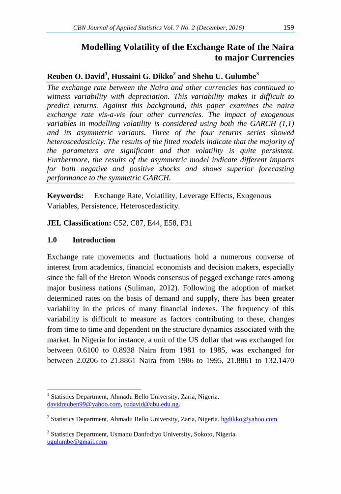
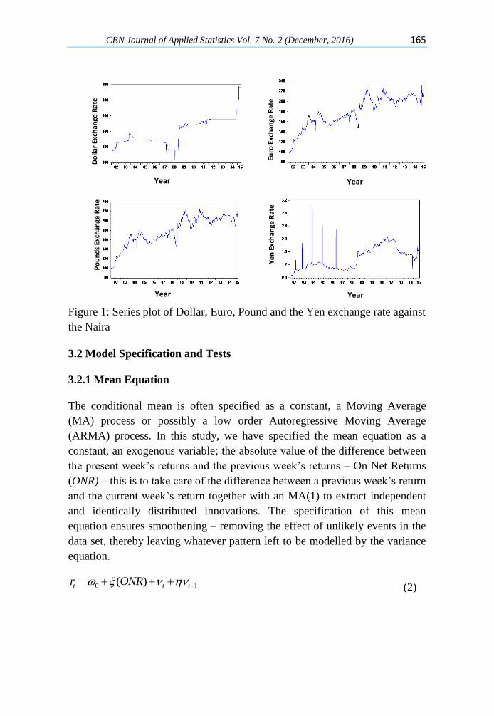
Figure 1 presents the time plots of the exchange rate of the naira. According to
Gujarati (2004) and Christoffersen (2012), unstable series such as these
cannot be used for further statistical inferences because of their implications.
This nonstationarity necessitates the transformation of the series.
3.1.1 Transformation
The exchange rate of each series was transformed to returns. In returns
estimation, there are both theoretical and empirical reasons for preferring
logarithmic returns. According to Strong (1992), theoretically, logarithmic
returns are analytically more tractable when linking together sub-period
returns to form returns over long intervals. Empirically, logarithmic returns
have much better statistical properties i.e. are more likely to be normally
distributed (Christoffersen, 2012). The weekly return is defined as:
1
ln tt
t
ya
y (1)
where at is the exchange rate return in period t and yt is the exchange rate in
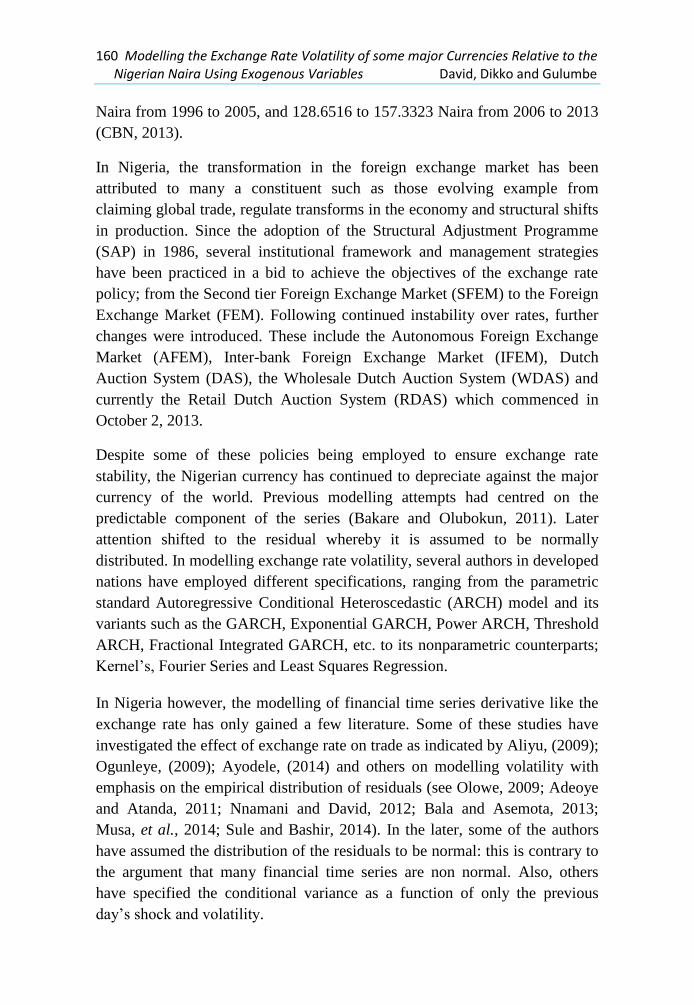
period t. The plot of the returns as shown in Figure 2 displays such
characteristic such as influential observations, volatility clustering and the
time varying pattern of the shocks.
CBN Journal of Applied Statistics Vol. 7 No. 2 (December, 2016) 165
Do
llar
Exch
ange
Rat
e
Euro
Exc
han
ge R
ate
Po
un
ds
Exch
ange
Rat
e
Ye
n E
xch
ange
Rat
e
Year Year
Year Year
Figure 1: Series plot of Dollar, Euro, Pound and the Yen exchange rate against
the Naira
3.2 Model Specification and Tests
3.2.1 Mean Equation
The conditional mean is often specified as a constant, a Moving Average
(MA) process or possibly a low order Autoregressive Moving Average
(ARMA) process. In this study, we have specified the mean equation as a
constant, an exogenous variable; the absolute value of the difference between
the present week’s returns and the previous week’s returns – On Net Returns
(ONR) – this is to take care of the difference between a previous week’s return
and the current week’s return together with an MA(1) to extract independent
and identically distributed innovations. The specification of this mean
equation ensures smoothening – removing the effect of unlikely events in the
data set, thereby leaving whatever pattern left to be modelled by the variance
equation.
0 1( )t t tr ONR (2)

166 Modelling the Exchange Rate Volatility of some major Currencies Relative to the Nigerian Naira Using Exogenous Variables David, Dikko and Gulumbe
Do
llar
Re
turn
s
Euro
Re
turn
s
Po
un
d R
etu
rns
Ye
n R
etu
rns
Year Year
Year Year
Figure 2: Stationary plot of Dollar, Euro, Pound and Yen Returns against the
Naira
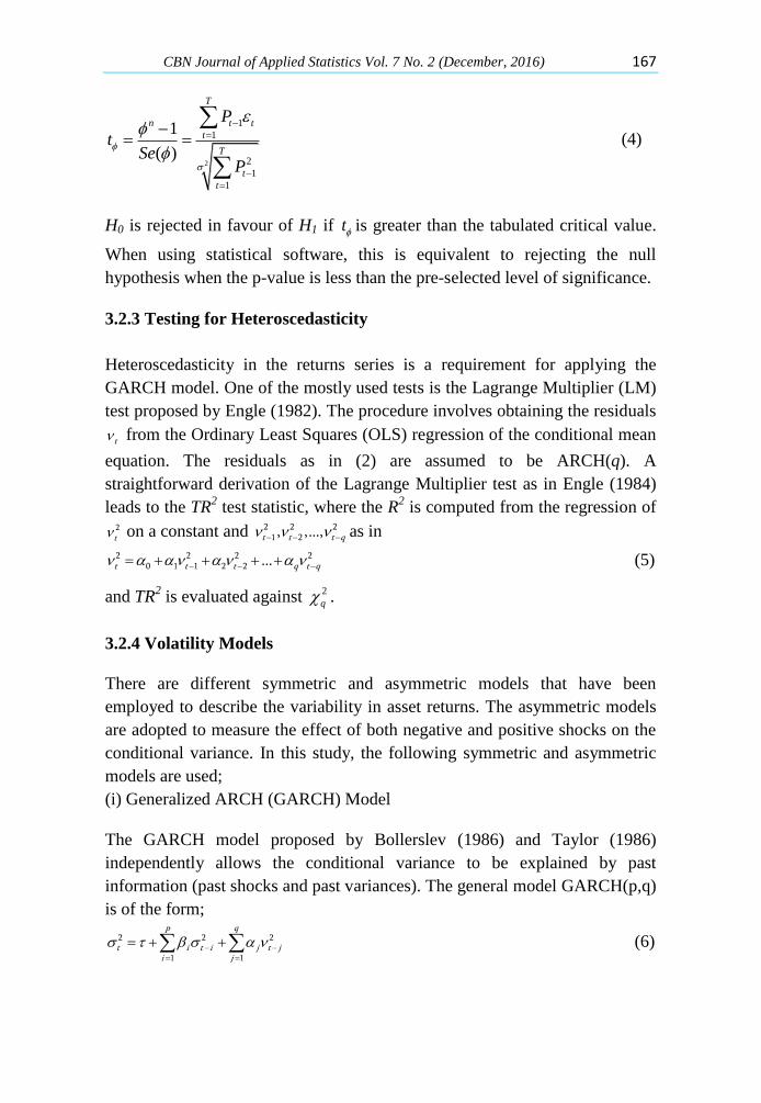
3.2.2 Stationarity Test
Achieving stationarity is a basic condition that must be satisfied before a
model can be selected. The Augmented Dickey Fuller (ADF) test used for
testing the presence of a unit root involves adding an unknown number of
lagged first differences of the dependent variable to capture autocorrelated
omitted variables that would otherwise, by default, enter the error term as in
the regression; '
1 1 1 2 2 ...t t t t t p t p ty y x y y y v (3)
where 1t t ty y y and '
tx are exogenous regressors. The approach tests the
hypotheses
0 : 1H (a series is nonstationary) against 1 : 1H (a series is stationary)
The hypothesis is evaluated using the t statistic for
CBN Journal of Applied Statistics Vol. 7 No. 2 (December, 2016) 167
2
1
1
2
1
1
1
( )
T
n t t
t
T
t
t
P
tSe
P
(4)
H0 is rejected in favour of H1 if t is greater than the tabulated critical value.
When using statistical software, this is equivalent to rejecting the null
hypothesis when the p-value is less than the pre-selected level of significance.
3.2.3 Testing for Heteroscedasticity
Heteroscedasticity in the returns series is a requirement for applying the
GARCH model. One of the mostly used tests is the Lagrange Multiplier (LM)
test proposed by Engle (1982). The procedure involves obtaining the residuals
t from the Ordinary Least Squares (OLS) regression of the conditional mean
equation. The residuals as in (2) are assumed to be ARCH(q). A
straightforward derivation of the Lagrange Multiplier test as in Engle (1984)
leads to the TR2 test statistic, where the R
2 is computed from the regression of
2t on a constant and
2 2 21 2, ,...,t t t q as in
2 2 2 20 1 1 2 2 ...t t t q t q (5)
and TR2 is evaluated against 2
q .
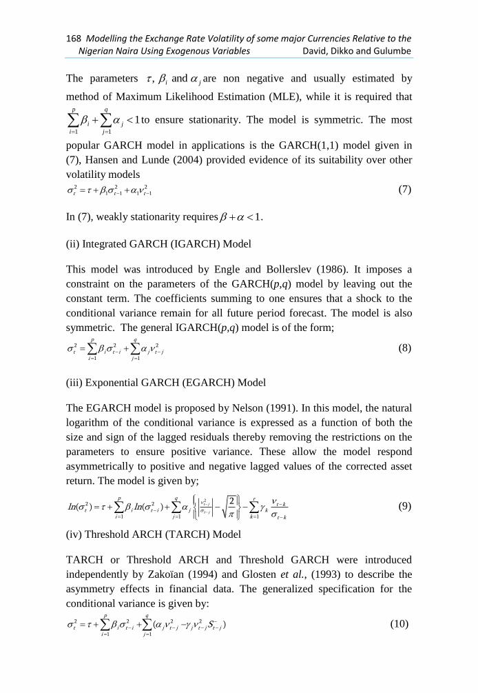
3.2.4 Volatility Models
There are different symmetric and asymmetric models that have been
employed to describe the variability in asset returns. The asymmetric models
are adopted to measure the effect of both negative and positive shocks on the
conditional variance. In this study, the following symmetric and asymmetric
models are used;
(i) Generalized ARCH (GARCH) Model
The GARCH model proposed by Bollerslev (1986) and Taylor (1986)
independently allows the conditional variance to be explained by past
information (past shocks and past variances). The general model GARCH(p,q)
is of the form;
2 2 2
1 1
p q
t i t i j t ji j
(6)
168 Modelling the Exchange Rate Volatility of some major Currencies Relative to the Nigerian Naira Using Exogenous Variables David, Dikko and Gulumbe
The parameters , and i j are non negative and usually estimated by
method of Maximum Likelihood Estimation (MLE), while it is required that
1 1
1p q
i j
i j
to ensure stationarity. The model is symmetric. The most
popular GARCH model in applications is the GARCH(1,1) model given in
(7), Hansen and Lunde (2004) provided evidence of its suitability over other
volatility models
2 2 21 1 1 1t t t (7)
In (7), weakly stationarity requires 1 .
(ii) Integrated GARCH (IGARCH) Model
This model was introduced by Engle and Bollerslev (1986). It imposes a
constraint on the parameters of the GARCH(p,q) model by leaving out the
constant term. The coefficients summing to one ensures that a shock to the
conditional variance remain for all future period forecast. The model is also
symmetric. The general IGARCH(p,q) model is of the form;
2 2 2
1 1
p q
t i t i j t ji j
(8)
(iii) Exponential GARCH (EGARCH) Model
The EGARCH model is proposed by Nelson (1991). In this model, the natural
logarithm of the conditional variance is expressed as a function of both the
size and sign of the lagged residuals thereby removing the restrictions on the
parameters to ensure positive variance. These allow the model respond
asymmetrically to positive and negative lagged values of the corrected asset
return. The model is given by;
22 2
1 1 1
2( ) ( ) t j
t j
p q rt k
t i t i j ki j k t k
ln ln (9)
(iv) Threshold ARCH (TARCH) Model
TARCH or Threshold ARCH and Threshold GARCH were introduced
independently by Zakoïan (1994) and Glosten et al., (1993) to describe the
asymmetry effects in financial data. The generalized specification for the
conditional variance is given by:
2 2 2 2
1 1
( )p q
t i t i j t j j t j t ji j
S (10)
CBN Journal of Applied Statistics Vol. 7 No. 2 (December, 2016) 169
where S is a dummy variable that is equal to 1 when 0t j and zero
otherwise. In this form of the model, good news 0t i has an effect of j on
volatility while bad news 0t i has an effect of ( )j j provided the
estimated parameter 0j . Eqn. (10) reduces to the GARCH model when
0t iS
.
(v) Power ARCH (PARCH) Model
This model introduced by Taylor (1986) and Schwert (1989) estimate the
parameter of the conditional volatility. The general specification of the model
is of the form;
1 1
( ) ( )p q
t i t i j t j j t ji j
(11)
where 0 , 1 1j . The estimation of the parameter rather than it
been imposed ensures the specification of the true distribution of the volatility
(Longmore and Robinson, 2004).
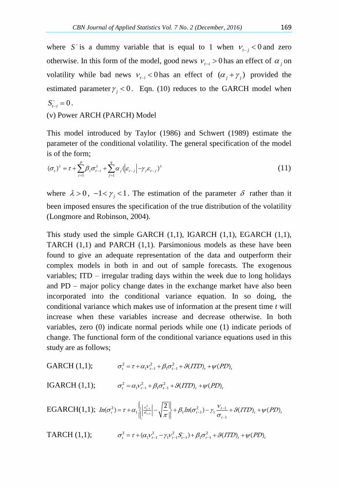
This study used the simple GARCH (1,1), IGARCH (1,1), EGARCH (1,1),
TARCH (1,1) and PARCH (1,1). Parsimonious models as these have been
found to give an adequate representation of the data and outperform their
complex models in both in and out of sample forecasts. The exogenous
variables; ITD – irregular trading days within the week due to long holidays
and PD – major policy change dates in the exchange market have also been
incorporated into the conditional variance equation. In so doing, the
conditional variance which makes use of information at the present time t will
increase when these variables increase and decrease otherwise. In both
variables, zero (0) indicate normal periods while one (1) indicate periods of
change. The functional form of the conditional variance equations used in this
study are as follows;
GARCH (1,1); 2 2 21 1 1 1 ( ) ( )t t t t tITD PD
IGARCH (1,1); 2 2 21 1 1 1 ( ) ( )t t t t tITD PD
EGARCH(1,1);
21
1
2 2 11 1 1 1
1
2( ) ( ) ( ) ( )t
t
tt t t t
t
ln ln ITD PD
TARCH (1,1);
2 2 2 21 1 1 1 1 1 1( ) ( ) ( )t t t t t t tS ITD PD

170 Modelling the Exchange Rate Volatility of some major Currencies Relative to the Nigerian Naira Using Exogenous Variables David, Dikko and Gulumbe
PARCH (1,1); 1 1 1 1 1 1( ) ( ) ( ) ( )t t t t t tITD PD
3.3 Estimation
GARCH models parameters are estimated by maximizing the likelihood
function constructed under the distribution of the residual term. The different
distributions that have been assumed for this innovation are the normal
(Gaussian) distribution, Student’s t-distribution, and the Generalized Error
Distribution (GED). The normal log-likelihood of parameter vector
( , , , , , , )T is
22
21 1
1 1( ) ( ) ( ln 2 ln )
2 2 2
T Tt
t t
t t t
L l
(12)
The maximization of (12) involves specifying the initial values of the
innovation (2
t ) and the conditional variance (2
t ). In this study, the
conditional distribution of the innovation has been specified as a Generalized
Error Distribution to capture all of the leptokurtosis present in the returns. The
functional form of this distribution is
1
2
( 1)( ; )
2 (1/ )
sx
X ss
sef x s
s
, where
1/ 22/2 (1/ )
(3/ )
s s
s
(13)
and the shape parameter s > 0. This distribution is a standard normal
distribution if s = 2 and fat-tailed if s < 2. The log likelihood function of (13)
is given by
1 2
1
1 1( ) log 1 log 2 log (1/ ) log
2 2
sn
tn t
t q t
sl s s
(14)
3.4 Model Selection
Standard selection criteria are the Akaike and Schwarz information criteria.
These criteria determine the size of the errors by evaluating the log-likelihood,
but also penalizes over fitting of models by including a penalty term (usually
twice the number of parameters used).
This study examined the Akaike Information Criteria with the form
CBN Journal of Applied Statistics Vol. 7 No. 2 (December, 2016) 171
2 lnRSS
AIC kn
(15)
where k = number of parameters fitted in the model, RSS = Residuals Sum of
Squares and n = number of observations in the series.
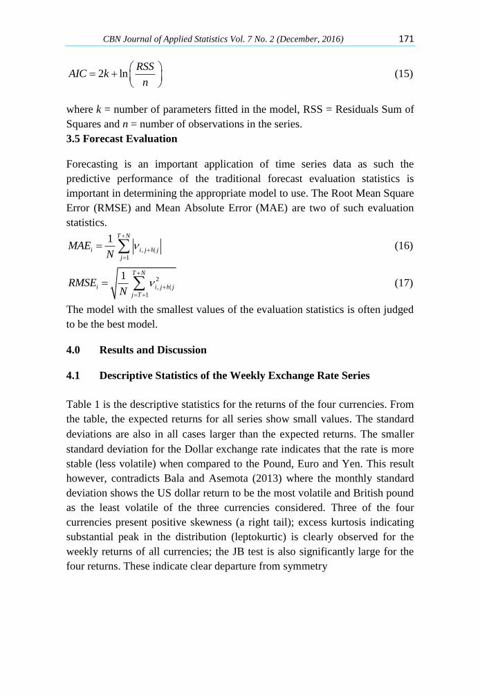
3.5 Forecast Evaluation
Forecasting is an important application of time series data as such the
predictive performance of the traditional forecast evaluation statistics is
important in determining the appropriate model to use. The Root Mean Square
Error (RMSE) and Mean Absolute Error (MAE) are two of such evaluation
statistics.
, |
1
1 T N
i i j h j
j
MAEN
(16)
2
, |
1
1 T N
i i j h j
j T
RMSEN
(17)
The model with the smallest values of the evaluation statistics is often judged
to be the best model.
4.0 Results and Discussion
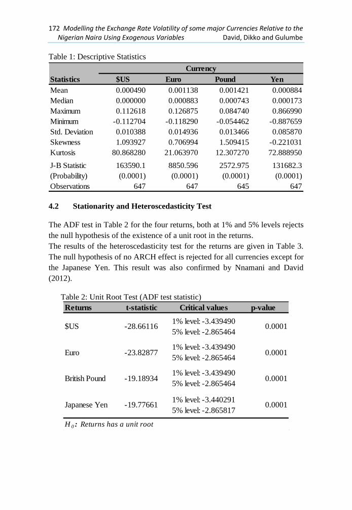
4.1 Descriptive Statistics of the Weekly Exchange Rate Series
Table 1 is the descriptive statistics for the returns of the four currencies. From
the table, the expected returns for all series show small values. The standard
deviations are also in all cases larger than the expected returns. The smaller
standard deviation for the Dollar exchange rate indicates that the rate is more
stable (less volatile) when compared to the Pound, Euro and Yen. This result
however, contradicts Bala and Asemota (2013) where the monthly standard
deviation shows the US dollar return to be the most volatile and British pound
as the least volatile of the three currencies considered. Three of the four
currencies present positive skewness (a right tail); excess kurtosis indicating
substantial peak in the distribution (leptokurtic) is clearly observed for the
weekly returns of all currencies; the JB test is also significantly large for the
four returns. These indicate clear departure from symmetry
172 Modelling the Exchange Rate Volatility of some major Currencies Relative to the Nigerian Naira Using Exogenous Variables David, Dikko and Gulumbe
Table 1: Descriptive Statistics
$US Euro Pound Yen
Mean 0.000490 0.001138 0.001421 0.000884
Median 0.000000 0.000883 0.000743 0.000173
Maximum 0.112618 0.126875 0.084740 0.866990
Minimum -0.112704 -0.118290 -0.054462 -0.887659
Std. Deviation 0.010388 0.014936 0.013466 0.085870
Skewness 1.093927 0.706994 1.509415 -0.221031
Kurtosis 80.868280 21.063970 12.307270 72.888950
J-B Statistic
(Probability)
163590.1
(0.0001)
8850.596
(0.0001)
2572.975
(0.0001)
131682.3
(0.0001)
Observations 647 647 645 647
Statistics
Currency
4.2 Stationarity and Heteroscedasticity Test
The ADF test in Table 2 for the four returns, both at 1% and 5% levels rejects
the null hypothesis of the existence of a unit root in the returns.
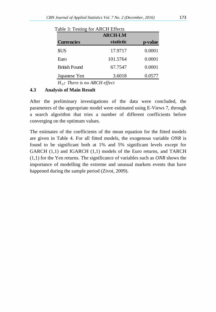
The results of the heteroscedasticity test for the returns are given in Table 3.
The null hypothesis of no ARCH effect is rejected for all currencies except for
the Japanese Yen. This result was also confirmed by Nnamani and David
(2012).
Table 2: Unit Root Test (ADF test statistic)
Returns t-statistic Critical values p-value
$US -28.661161% level: -3.439490
5% level: -2.8654640.0001
Euro -23.828771% level: -3.439490
5% level: -2.8654640.0001
British Pound -19.189341% level: -3.439490
5% level: -2.8654640.0001
Japanese Yen -19.776611% level: -3.440291
5% level: -2.8658170.0001
H 0 : Returns has a unit root
CBN Journal of Applied Statistics Vol. 7 No. 2 (December, 2016) 173
Table 3: Testing for ARCH Effects
Currencies
ARCH-LM
statistic p-value
$US 17.9717 0.0001
Euro 101.5764 0.0001
British Pound 67.7547 0.0001
Japanese Yen 3.6018 0.0577
H 0 : There is no ARCH effect 4.3 Analysis of Main Result
After the preliminary investigations of the data were concluded, the
parameters of the appropriate model were estimated using E-Views 7, through
a search algorithm that tries a number of different coefficients before
converging on the optimum values.
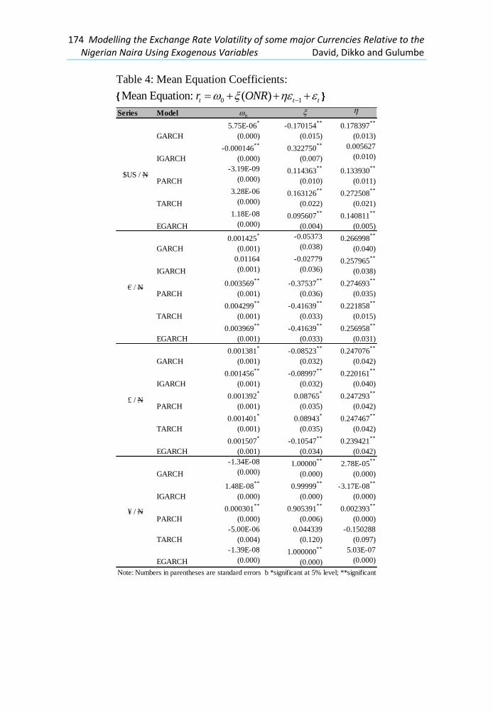
The estimates of the coefficients of the mean equation for the fitted models
are given in Table 4. For all fitted models, the exogenous variable ONR is
found to be significant both at 1% and 5% significant levels except for
GARCH (1,1) and IGARCH (1,1) models of the Euro returns, and TARCH
(1,1) for the Yen returns. The significance of variables such as ONR shows the
importance of modelling the extreme and unusual markets events that have
happened during the sample period (Zivot, 2009).
174 Modelling the Exchange Rate Volatility of some major Currencies Relative to the Nigerian Naira Using Exogenous Variables David, Dikko and Gulumbe
Table 4: Mean Equation Coefficients:
{ 0 1Mean Equation: ( )t t tr ONR }
Series Model
GARCH
5.75E-06*
(0.000)
-0.170154**
(0.015)
0.178397**
(0.013)
IGARCH
-0.000146**
(0.000)
0.322750**
(0.007)
0.005627
(0.010)
PARCH
-3.19E-09
(0.000)0.114363
**
(0.010)
0.133930**
(0.011)
TARCH
3.28E-06
(0.000)0.163126
**
(0.022)
0.272508**
(0.021)
EGARCH
1.18E-08
(0.000)0.095607
**
(0.004)
0.140811**
(0.005)
GARCH
0.001425*
(0.001)
-0.05373
(0.038)0.266998
**
(0.040)
IGARCH
0.01164
(0.001)
-0.02779
(0.036)0.257965
**
(0.038)
PARCH
0.003569**
(0.001)
-0.37537**
(0.036)
0.274693**
(0.035)
TARCH
0.004299**
(0.001)
-0.41639**
(0.033)
0.221858**
(0.015)
EGARCH
0.003969**
(0.001)
-0.41639**
(0.033)
0.256958**
(0.031)
GARCH
0.001381*
(0.001)
-0.08523**
(0.032)
0.247076**
(0.042)
IGARCH
0.001456**
(0.001)
-0.08997**
(0.032)
0.220161**
(0.040)
PARCH
0.001392*
(0.001)
0.08765*
(0.035)
0.247293**
(0.042)
TARCH
0.001401*
(0.001)
0.08943*
(0.035)
0.247467**
(0.042)
EGARCH
0.001507*
(0.001)
-0.10547**
(0.034)
0.239421**
(0.042)
GARCH
-1.34E-08
(0.000)1.00000
**
(0.000)
2.78E-05**
(0.000)
IGARCH
1.48E-08**
(0.000)
0.99999**
(0.000)
-3.17E-08**
(0.000)
PARCH
0.000301**
(0.000)
0.905391**
(0.006)
0.002393**
(0.000)
TARCH
-5.00E-06
(0.004)
0.044339
(0.120)
-0.150288
(0.097)
EGARCH
-1.39E-08
(0.000)1.000000
**
(0.000)
5.03E-07
(0.000)
Note: Numbers in parentheses are standard errors b *significant at 5% level; **significant at 1% level.
$US / N
€ / N
£ / N
¥ / N
0

CBN Journal of Applied Statistics Vol. 7 No. 2 (December, 2016) 175
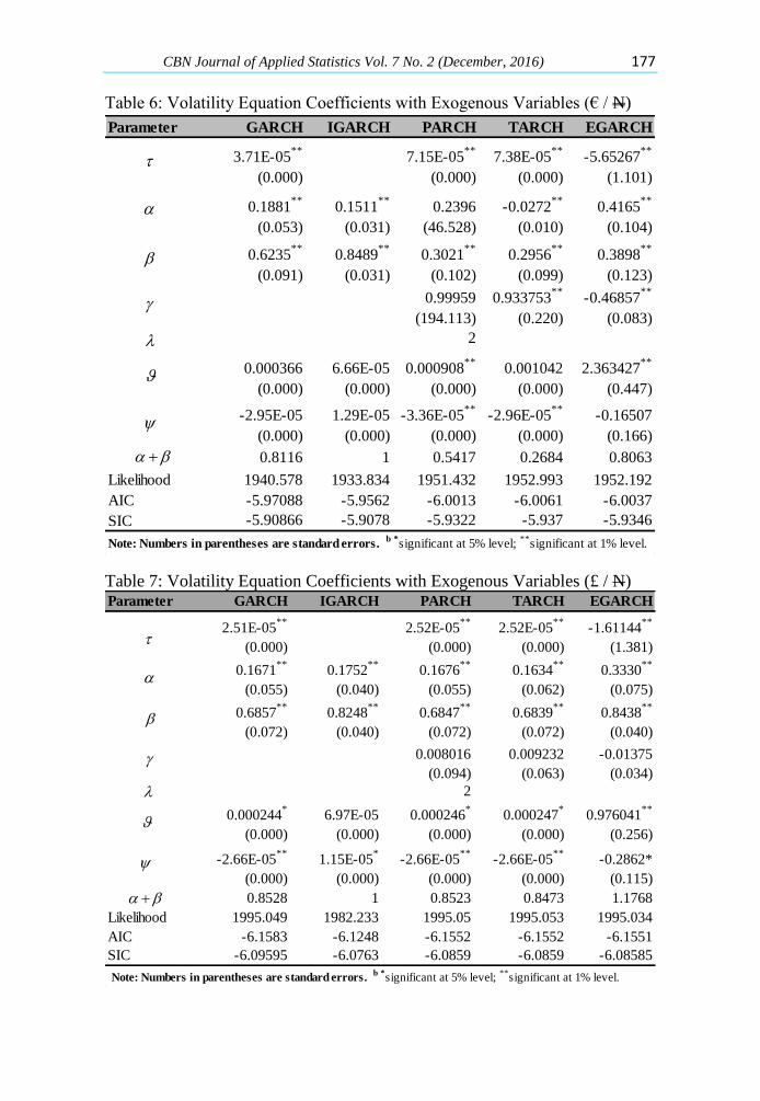
In Tables 5, 6, and 7 are the estimates of the parameters for the three
currencies’ returns.
From these tables, it can be concluded that the coefficients (constant), α
(ARCH) and β (GARCH) are statistically significant at both 1% and 5%
levels of significance for the Dollar, Euro and Pounds with expected sign for
all return series. The only notable exception is the ARCH term (α) of the
PARCH (1,1) model for the Euro series which is statistically insignificant
even at the 5% level. Similar result was obtained by Olowe (2009) for the
$US/N return for fixed and managed float regime. This is in contrast with
Insah (2013) where negative and positive significant values were obtained for
α and β respectively.
The significance of both α and β indicates that, news about volatility (i.e.,
fluctuation) from the previous periods have an explanatory power on current
volatility. According to Longmore and Robinson (2004), positive values for
these coefficients suggests that as the market approaches expected future rate,
volatility will tend to increase. In some of the models, the coefficients of α
and β were high while at other times they are low. The high value of β
indicates that shocks to the conditional variance are persistent while high
value of α indicates that volatility adjusts quickly to changes in the market.
The leverage coefficient , is significant for the PARCH (1,1), TARCH (1,1),
and EGARCH (1,1) in the Dollar returns, EGARCH (1,1) in Euro returns and
EGARCH (1,1) in Pound returns with expected sign and positive in TARCH
(1,1) in Euro returns. The negative sign and significance of indicates that
negative shock causes volatility to rise more than if a positive shock with the
same magnitude had occurred.
The parameters of the incorporated explanatory variables and for
irregular trading days and policy change dates respectively are found to be
statistically significant for majority of the fitted models for the three returns.
While the estimates of are positive, the estimates of are mostly negative.
This is consistent with the study of Bala and Asemota (2013) where they
found estimates of to be negative and responsible for reduction in
persistence
The estimated persistence coefficient (α + β) for the GARCH (1,1) model is
calculated for all the time series. The persistence coefficient for the Euro and
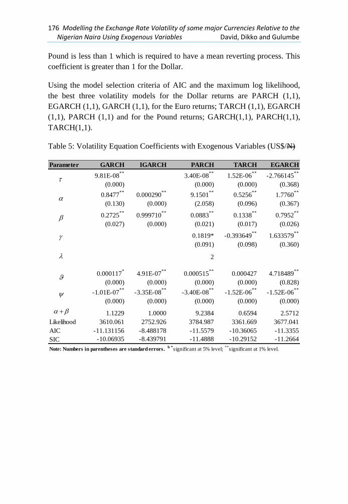
176 Modelling the Exchange Rate Volatility of some major Currencies Relative to the Nigerian Naira Using Exogenous Variables David, Dikko and Gulumbe
Pound is less than 1 which is required to have a mean reverting process. This
coefficient is greater than 1 for the Dollar.
Using the model selection criteria of AIC and the maximum log likelihood,
the best three volatility models for the Dollar returns are PARCH (1,1),
EGARCH (1,1), GARCH (1,1), for the Euro returns; TARCH (1,1), EGARCH
(1,1), PARCH (1,1) and for the Pound returns; GARCH(1,1), PARCH(1,1),
TARCH(1,1).
Table 5: Volatility Equation Coefficients with Exogenous Variables (US$/N)
Parameter GARCH IGARCH PARCH TARCH EGARCH
9.81E-08**
(0.000)
3.40E-08**
(0.000)
1.52E-06**
(0.000)
-2.766145**
(0.368)
0.8477**
(0.130)
0.000290**
(0.000)
9.1501**
(2.058)
0.5256**
(0.096)
1.7760**
(0.367)
Likelihood 3610.061 2752.926 3784.987 3361.669 3677.041
AIC -11.131156 -8.488178 -11.5579 -10.36065 -11.3355
SIC -10.06935 -8.439791 -11.4888 -10.29152 -11.2664
Note: Numbers in parentheses are standard errors. b *significant at 5% level;
**significant at 1% level.
0.2725**
(0.027)
0.999710**
(0.000)
0.0883**
(0.021)
0.1338**
(0.017)
0.7952**
(0.026)
0.1819*
(0.091)
-0.393649**
(0.098)
1.633579**
(0.360)
2
0.000117*
(0.000)
4.91E-07**
(0.000)
0.000515**
(0.000)
0.000427
(0.000)
4.718489**
(0.828)
-1.01E-07**
(0.000)
-3.35E-08**
(0.000)
-3.40E-08**
(0.000)
-1.52E-06**
(0.000)
-1.52E-06**
(0.000)
1.1229 1.0000 9.2384 0.6594 2.5712
CBN Journal of Applied Statistics Vol. 7 No. 2 (December, 2016) 177
Table 6: Volatility Equation Coefficients with Exogenous Variables (€ / N)
Parameter GARCH IGARCH PARCH TARCH EGARCH
3.71E-05**
(0.000)
7.15E-05**
(0.000)
7.38E-05**
(0.000)
-5.65267**
(1.101)
0.1881**
(0.053)
0.1511**
(0.031)
0.2396
(46.528)
-0.0272**
(0.010)
0.4165**
(0.104)
0.6235**
(0.091)
0.8489**
(0.031)
0.3021**
(0.102)
0.2956**
(0.099)
0.3898**
(0.123)
0.99959
(194.113)
0.933753**
(0.220)
-0.46857**
(0.083)
2
0.000366
(0.000)
6.66E-05
(0.000)
0.000908**
(0.000)
0.001042
(0.000)
2.363427**
(0.447)
-2.95E-05
(0.000)
1.29E-05
(0.000)
-3.36E-05**
(0.000)
-2.96E-05**
(0.000)
-0.16507
(0.166)
0.8116 1 0.5417 0.2684 0.8063
Likelihood 1940.578 1933.834 1951.432 1952.993 1952.192
AIC -5.97088 -5.9562 -6.0013 -6.0061 -6.0037
SIC -5.90866 -5.9078 -5.9322 -5.937 -5.9346
Note: Numbers in parentheses are standard errors. b *significant at 5% level;
**significant at 1% level.
Table 7: Volatility Equation Coefficients with Exogenous Variables (£ / N) Parameter GARCH IGARCH PARCH TARCH EGARCH
2.51E-05**
(0.000)
2.52E-05**
(0.000)
2.52E-05**
(0.000)
-1.61144**
(1.381)
0.1671**
(0.055)
0.1752**
(0.040)
0.1676**
(0.055)
0.1634**
(0.062)
0.3330**
(0.075)
Likelihood 1995.049 1982.233 1995.05 1995.053 1995.034
AIC -6.1583 -6.1248 -6.1552 -6.1552 -6.1551
SIC -6.09595 -6.0763 -6.0859 -6.0859 -6.08585
Note: Numbers in parentheses are standard errors. b *significant at 5% level;
**significant at 1% level.
0.6857**
(0.072)
0.8248**
(0.040)
0.6847**
(0.072)
0.6839**
(0.072)
0.8438**
(0.040)
0.008016
(0.094)
0.009232
(0.063)
-0.01375
(0.034)
2
0.000244*
(0.000)
6.97E-05
(0.000)
0.000246*
(0.000)
0.000247*
(0.000)
0.976041**
(0.256)
-2.66E-05**
(0.000)
1.15E-05*
(0.000)
-2.66E-05**
(0.000)
-2.66E-05**
(0.000)
-0.2862*
(0.115)
0.8528 1 0.8523 0.8473 1.1768
178 Modelling the Exchange Rate Volatility of some major Currencies Relative to the Nigerian Naira Using Exogenous Variables David, Dikko and Gulumbe
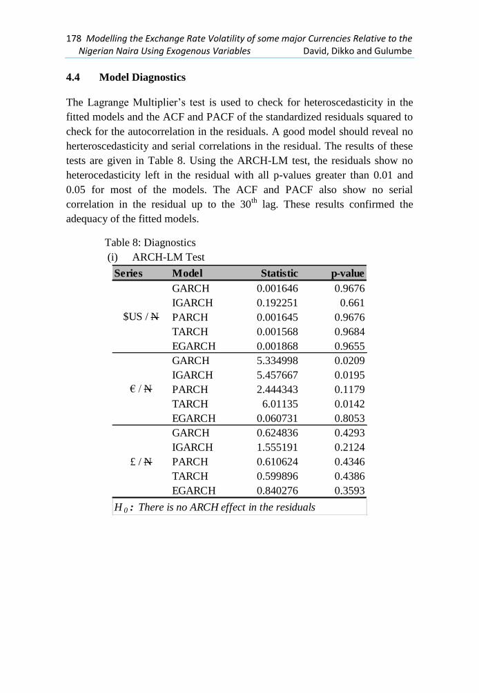
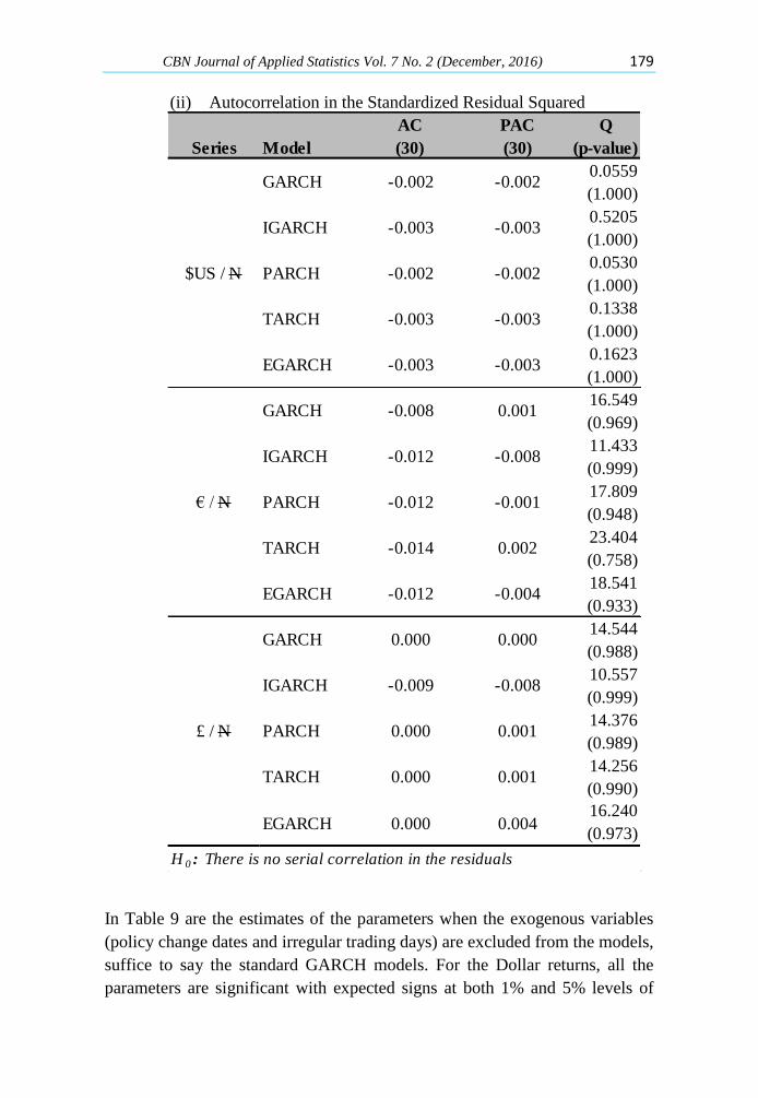
4.4 Model Diagnostics
The Lagrange Multiplier’s test is used to check for heteroscedasticity in the
fitted models and the ACF and PACF of the standardized residuals squared to
check for the autocorrelation in the residuals. A good model should reveal no
herteroscedasticity and serial correlations in the residual. The results of these
tests are given in Table 8. Using the ARCH-LM test, the residuals show no
heterocedasticity left in the residual with all p-values greater than 0.01 and
0.05 for most of the models. The ACF and PACF also show no serial
correlation in the residual up to the 30th
lag. These results confirmed the
adequacy of the fitted models.
Table 8: Diagnostics
(i) ARCH-LM Test
Series Model Statistic p-value
GARCH 0.001646 0.9676
IGARCH 0.192251 0.661
PARCH 0.001645 0.9676
TARCH 0.001568 0.9684
EGARCH 0.001868 0.9655
GARCH 5.334998 0.0209
IGARCH 5.457667 0.0195
PARCH 2.444343 0.1179
TARCH 6.01135 0.0142
EGARCH 0.060731 0.8053
GARCH 0.624836 0.4293
IGARCH 1.555191 0.2124
PARCH 0.610624 0.4346
TARCH 0.599896 0.4386
EGARCH 0.840276 0.3593
H 0 : There is no ARCH effect in the residuals
$US / N
€ / N
£ / N
CBN Journal of Applied Statistics Vol. 7 No. 2 (December, 2016) 179
(ii) Autocorrelation in the Standardized Residual Squared
GARCH -0.002 -0.0020.0559
(1.000)
IGARCH -0.003 -0.0030.5205
(1.000)
PARCH -0.002 -0.0020.0530
(1.000)
TARCH -0.003 -0.0030.1338
(1.000)
EGARCH -0.003 -0.0030.1623
(1.000)
GARCH -0.008 0.00116.549
(0.969)
IGARCH -0.012 -0.00811.433
(0.999)
PARCH -0.012 -0.00117.809
(0.948)
TARCH -0.014 0.00223.404
(0.758)
EGARCH -0.012 -0.00418.541
(0.933)
GARCH 0.000 0.00014.544
(0.988)
IGARCH -0.009 -0.00810.557
(0.999)
PARCH 0.000 0.00114.376
(0.989)
TARCH 0.000 0.00114.256
(0.990)
EGARCH 0.000 0.00416.240
(0.973)
H 0 : There is no serial correlation in the residuals
PAC
(30)
Q
(p-value)
$US / N
€ / N
£ / N
AC
(30)Series Model
In Table 9 are the estimates of the parameters when the exogenous variables
(policy change dates and irregular trading days) are excluded from the models,
suffice to say the standard GARCH models. For the Dollar returns, all the
parameters are significant with expected signs at both 1% and 5% levels of
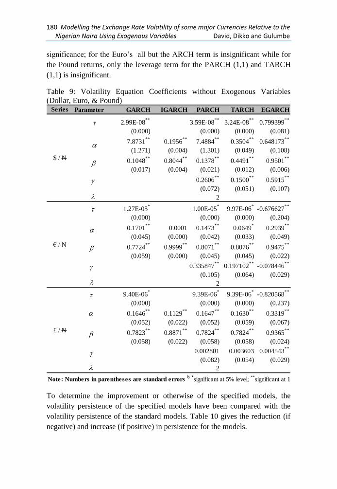
180 Modelling the Exchange Rate Volatility of some major Currencies Relative to the Nigerian Naira Using Exogenous Variables David, Dikko and Gulumbe
significance; for the Euro’s all but the ARCH term is insignificant while for
the Pound returns, only the leverage term for the PARCH (1,1) and TARCH
(1,1) is insignificant.
Table 9: Volatility Equation Coefficients without Exogenous Variables
(Dollar, Euro, & Pound) Series Parameter GARCH IGARCH PARCH TARCH EGARCH
2.99E-08**
(0.000)
3.59E-08**
(0.000)
3.24E-08**
(0.000)
0.799399**
(0.081)
0.1048**
(0.017)
0.8044**
(0.004)
0.1378**
(0.021)
0.4491**
(0.012)
0.9501**
(0.006)
0.2606**
(0.072)
0.1500**
(0.051)
0.5915**
(0.107)
2
1.27E-05*
(0.000)
1.00E-05*
(0.000)
9.97E-06*
(0.000)
-0.676627**
(0.204)
0.7724**
(0.059)
0.9999**
(0.000)
0.8071**
(0.045)
0.8076**
(0.045)
0.9475**
(0.022)
0.335847**
(0.105)
0.197102**
(0.064)
-0.078446**
(0.029)
2
9.40E-06*
(0.000)
9.39E-06*
(0.000)
9.39E-06*
(0.000)
-0.820568**
(0.237)
0.7823**
(0.058)
0.8871**
(0.022)
0.7824**
(0.058)
0.7824**
(0.058)
0.9365**
(0.024)
0.002801
(0.082)
0.003603
(0.054)
0.004543**
(0.029)
2
Note: Numbers in parentheses are standard errors b *significant at 5% level;
**significant at 1% level.
7.8731**
(1.271)
0.1956**
(0.004)
7.4884**
(1.301)
0.3504**
(0.049)
0.648173**
(0.108)
€ / N
0.1701**
(0.045)
0.0001
(0.000)
0.1473**
(0.042)
0.0649*
(0.033)
0.2939**
(0.049)
$ / N
0.3319**
(0.067)
£ / N
0.1646**
(0.052)
0.1129**
(0.022)
0.1647**
(0.052)
0.1630**
(0.059)
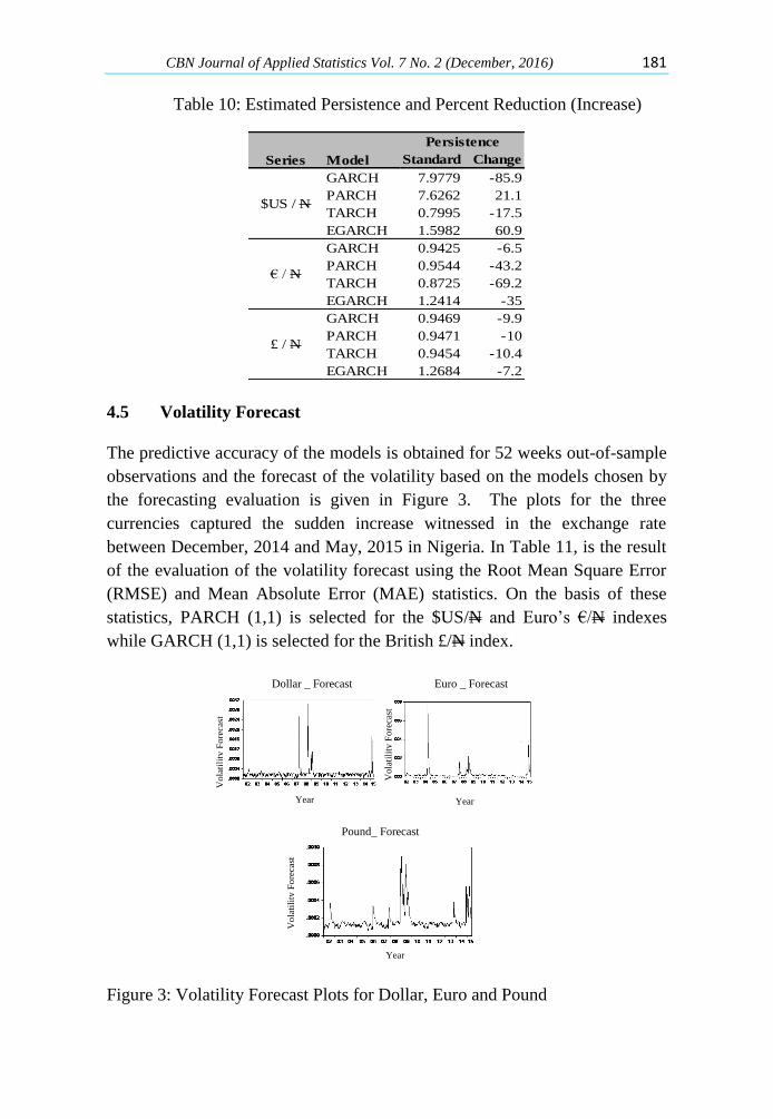
To determine the improvement or otherwise of the specified models, the
volatility persistence of the specified models have been compared with the
volatility persistence of the standard models. Table 10 gives the reduction (if
negative) and increase (if positive) in persistence for the models.
CBN Journal of Applied Statistics Vol. 7 No. 2 (December, 2016) 181
Table 10: Estimated Persistence and Percent Reduction (Increase)
Standard Change
GARCH 7.9779 -85.9
PARCH 7.6262 21.1
TARCH 0.7995 -17.5
EGARCH 1.5982 60.9
GARCH 0.9425 -6.5
PARCH 0.9544 -43.2
TARCH 0.8725 -69.2
EGARCH 1.2414 -35
GARCH 0.9469 -9.9
PARCH 0.9471 -10
TARCH 0.9454 -10.4
EGARCH 1.2684 -7.2
Series Model
Persistence
$US / N
€ / N
£ / N
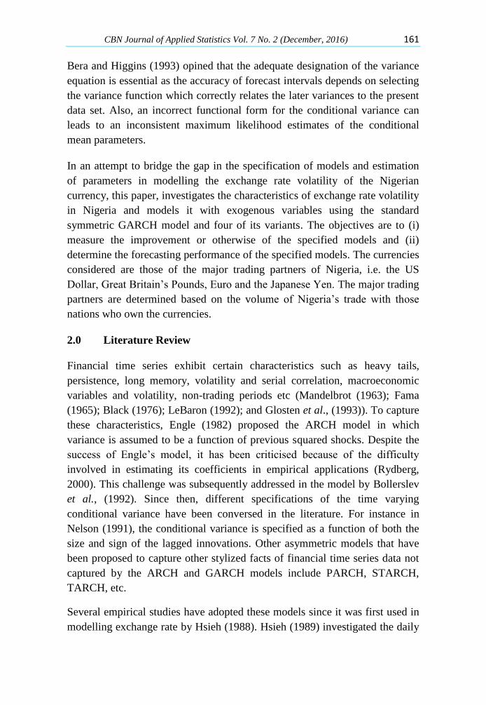
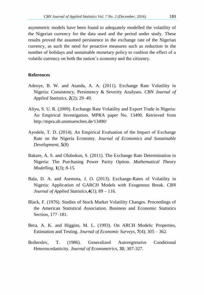
4.5 Volatility Forecast
The predictive accuracy of the models is obtained for 52 weeks out-of-sample
observations and the forecast of the volatility based on the models chosen by
the forecasting evaluation is given in Figure 3. The plots for the three
currencies captured the sudden increase witnessed in the exchange rate
between December, 2014 and May, 2015 in Nigeria. In Table 11, is the result
of the evaluation of the volatility forecast using the Root Mean Square Error
(RMSE) and Mean Absolute Error (MAE) statistics. On the basis of these
statistics, PARCH (1,1) is selected for the $US/N and Euro’s €/N indexes
while GARCH (1,1) is selected for the British £/N index.
Year
Po
un
d F
ore
cast
Vo
lati
lity
Fo
reca
st
Vo
lati
lity
Fo
reca
st
Vo
lati
lity
Fo
reca
st
Dollar _ Forecast Euro _ Forecast
Pound_ Forecast
Year Year
Year
Figure 3: Volatility Forecast Plots for Dollar, Euro and Pound

182 Modelling the Exchange Rate Volatility of some major Currencies Relative to the Nigerian Naira Using Exogenous Variables David, Dikko and Gulumbe
Table 11: Volatility Forecasting Evaluation
Series Model RMSE MAE
PARCH 0.01681 0.00472
EGARCH 0.01695 0.00473
GARCH 0.01957 0.00551
TARCH 0.0277 0.01503
EGARCH 0.02796 0.01504
PARCH 0.02724 0.01456
GARCH 0.02259 0.01198
PARCH 0.02261 0.01198
TARCH 0.02263 0.01198
$US / N
€ / N
£ / N
5.0 Conclusion
This study examined the symmetric GARCH (1,1) model and its asymmetric
variants to investigates the volatility of the Nigerian currency vis-à-vis the
currency of its major trading partners. We used weekly data for the exchange
rate of the four currencies; $US against N, the European € against N, the
British £ against N, and the Japanese Yen (¥) against N. The special feature of
the models used in this study is that the series volatility has been modelled as
a function of the standard GARCH parameters and two exogenous variables.
The fitted models remove the serial correlation and heteroscedasticity in the
residual. The results also showed that the conditional variance is an explosive
process for the Dollar currency ( > 1) while it is quite persistent (
< 1) for the Pound and Euro currencies. The explosive volatility observed in
the Dollar currency could be attributed to it being the dominant reserve
currency in financial markets. This result is in consonance with those of other
developing markets where significant persistence of volatility is observed for
the US Dollar.
For the exogenous variables used in this study, while ITD tends to increase the
volatility of the Naira, PD leads to a reduction in the estimated volatility
persistence. This imply that the greater the number of non – trading days in a
week, the more volatile the exchange rate between the Naira and the Dollar,
Euro and Pound currencies. Also, the different policy change dates of the
government resulted in lower volatility of the exchange rate. The forecasting
performance of the fitted model in both in-sample and out-sample showed the
PARCH (1,1) to have a better predictive performance for the Dollar’s and
Euro’s series while GARCH (1,1) is chosen for the Pound’s series. The
CBN Journal of Applied Statistics Vol. 7 No. 2 (December, 2016) 183
asymmetric models have been found to adequately modelled the volatility of
the Nigerian currency for the data used and the period under study. These
results proved the assumed persistence in the exchange rate of the Nigerian
currency, as such the need for proactive measures such as reduction in the
number of holidays and sustainable monetary policy to cushion the effect of a
volatile currency on both the nation’s economy and the citizenry.
References
Adeoye, B. W. and Atanda, A. A. (2011). Exchange Rate Volatility in
Nigeria: Consistency, Persistency & Severity Analyses. CBN Journal of
Applied Statistics, 2(2); 29–49.
Aliyu, S. U. R. (2009). Exchange Rate Volatility and Export Trade in Nigeria:
An Empirical Investigation. MPRA paper No. 13490. Retrieved from
http://mpra.ub.unimuenchen.de/13490/
Ayodele, T. D. (2014). An Empirical Evaluation of the Impact of Exchange
Rate on the Nigeria Economy. Journal of Economics and Sustainable
Development, 5(8)
Bakare, A. S. and Olubokun, S. (2011). The Exchange Rate Determination in
Nigeria: The Purchasing Power Parity Option. Mathematical Theory
Modelling, 1(3); 8-15.
Bala, D. A. and Asemota, J. O. (2013). Exchange-Rates of Volatility in
Nigeria: Application of GARCH Models with Exogenous Break. CBN
Journal of Applied Statistics,4(1); 89 – 116.
Black, F. (1976). Studies of Stock Market Volatility Changes. Proceedings of
the American Statistical Association. Business and Economic Statistics
Section, 177–181.
Bera, A. K. and Higgins, M. L. (1993). On ARCH Models: Properties,
Estimation and Testing. Journal of Economic Surveys, 7(4); 305 – 362.
Bollerslev, T. (1986). Generalized Autoregressive Conditional
Heteroscedasticity. Journal of Econometrics, 31; 307-327.
184 Modelling the Exchange Rate Volatility of some major Currencies Relative to the Nigerian Naira Using Exogenous Variables David, Dikko and Gulumbe
Bollerslev, T., Chou, R. Y. and Kroner, K. F. (1992). ARCH Modeling in
Finance: A Review of the Theory and Empirical Evidence. Journal of
Econometrics, (52); 5-59.
Central Bank of Nigeria (2013). Statistical Bulletin, 24; 221-230
Christoffersen, P. F. (2012). Elements of Financial Risk Management. Oxford.
Elsevier, Inc.
Cont, R. (2001). “Empirical Properties of Asset Returns: Stylized Facts and
Statistical Issues”. Quantitative Finance, 1(2); 223-236.
Engle, R. F. (1982). “Autoregressive Conditional Heteroscedasticity with
Estimates of the Variance of the United Kingdom Inflation”,
Econometrica, 5; 987-1008.
Engle, R. F. and Patton, A. J. (2001). What good is a Volatility Model?
Quantitative Finance, 1(2); 237 – 245.
Erdemlioglu, D., Laurent, S. and Neely, C. J. (2012). Econometric Modelling
of Exchange Rate Volatility and Jumps. Working Paper 2012-008A.
Fama, E. F. (1965). The Behavior of Stock Market Prices. Journal of
Business, 38; 34–105.
Flannery, M. and Protopapadakis, A. (2002). Macroeconomic Factors Do
Influence Aggregate Stock Returns. The Review of Financial Studies, 15;
751-782.
Gallo, G. M. and Pacini, B. (1998). Early News is Good News: The Effects of
Market Opening on Market Volatility. Studies in Nonlinear Dynamics and
Econometrics, Quarterly Journal, 2(4); 115 – 131.
Glosten, L. R., Jagannathan, R. and Runkle, D. E. (1993).On the Relation
between the Expected Value and the Volatility of the Nominal Excess
Returns on Stocks. Journal of Finance, 48(5); 1779-1791.
Gujarati, D. N. (2004) Basic Econometrics. New, Delhi. Tata McGraw Hill
Publishing Company Limited.
CBN Journal of Applied Statistics Vol. 7 No. 2 (December, 2016) 185
Hansen, P. and Lunde, A. (2004). A Forecast Comparison of Volatility
Models: Does Anything Beat a GARCH(1,1) Model? Journal of Applied
Econometrics 20; 873-889.
Hsieh, D. A. (1988). The Statistical Properties of Daily Foreign Exchange
Rates: 1974 – 1983. Journal of International Economics, 24(1-2); 129 –
145.
Hsieh D. A. (1989). Modeling Heteroscedasticity in Daily Foreign-Exchange
Rates. Journal of Business and Economic Statistics, 7; 307-317.
Insah, B. (2013). Modelling Real Exchange Rate Volatility in a Developing
Country. Journal of Economics and Sustainable Development, 4(6); 61-69.
Lamoureux, C. G. and Lastrapes, W. D. (1990). Heteroskedasticity in Stock
Return Data: Volume versus GARCH effects. The Journal of Finance, 45;
221–229.
Laurent, S., Rombouts, J. and Violante F. (2011). On the Forecsating
Accuracy of Multivariate GARCH Models, forthcoming in Journal of
Applied Econometrics.
Lastrapes, W. D. (1989). Exchange Rate Volatility and U.S. Monetary Policy:
An ARCH Application. Journal of Money, Credit Banking, 21; 66-77.
LeBaron, B. (1992). Some Relations between Volatility and Serial Correlation
in Stock Market Returns. Journal of Business, 65; 199-220.
Longmore, R. and Robinson, W. (2004). Modelling and Forecasting Exchange
Rate Dynamics: An Application of Asymmetric Volatility Models. Bank of
Jamaica. Working Paper WP2004/03.
Mandelbrot, B. (1963). The Variation of certain Speculative Prices. Journal of
Business, 36; 394-414.
Musa, Y. and Abubakar, B. (2014). Investigating Daily/Dollar Exchange Rate
Volatility: A Modelling Using GARCH and Asymmetric Models. IOSR
Journal of Mathematics, 10(2); 139 -148.
Musa, Y., Tasi’u, M. and Abubakar, B. (2014). Forecasting of Exchange Rate
Volatility between Naira and US Dollar Using GARCH Models.
International Journal of Academic Research in Business and Social
Sciences, 4(7); 369 – 381.
186 Modelling the Exchange Rate Volatility of some major Currencies Relative to the Nigerian Naira Using Exogenous Variables David, Dikko and Gulumbe
Nelson, D. B. (1991). Conditional Heteroscedasticity in Asset Returns: A New
Approach. Econometrica, 59; 347–370.
Nnamani, C. N. and David, R. O. (2012). Modelling Exchange Rate
Volatility: The Nigerian Foreign Exchange Market Experience. LAP
Lambert Academic Publishers, AV Akademikerverlag GmbH & Co,
Germany.
Ogunleye, E. R. (2009). Exchange Rate Volatility and Foreign Direct
Investment in Sub-Saharan Africa: Evidence from Nigeria and South
Africa.
In. Adeola Adenikinju, Dipo Busari and Sam Olofin (ed.) Applied
Econometrics and Macroeconomic Modelling in Nigeria. Ibadan
University Press.
Olowe, R. A. (2009). Modelling Naira/Dollar Exchange Rate Volatility:
Application of GARCH and Asymmetric Models. International Review of
Business Research Papers, 5(3); 377 – 398.
Rydberg, T. H. (2000). Realistic Statistical Modelling of Financial Data.
International Statistical Review, 68(3); 233 – 258.
Schwert, W. (1989). Stock Volatility and Crash of ’87. Review of Financial
Studies, 3; 77–102.
Strong, N. (1992). Modelling Abnormal Returns: A Review Article. Journal
of Business Finance and Accounting, 19(4); 533–553.
Sule, A. A. and Bashir, A. M. (2014). Volatility Modelling of Daily Exchange
Rate between the United States Dollar and Nigeria Naira. Annual
Conference Proceedings of the Nigerian Statistical Association, 54 – 64.
Suliman, Z. S. A. (2012). Modelling Exchange Rate Volatility using GARCH
Models: Empirical Evidence from Arab countries. International Journal of
Economics and Finance, 4; 216-229.
Taylor, S. J. (1986). Modelling Financial Time Series. New York. John Wiley
and Sons Inc.
Zakoïan, J. M. (1994). Threshold Heteroskedastic Models, Journal of
Economic Dynamics and Control, 18; 931-944.

CBN Journal of Applied Statistics Vol. 7 No. 2 (December, 2016) 187
Zivot, E. (2009). Practical Issues in the Analysis of Univariate GARCH
Models.
In Andersen, T.G., Davis, R.A., Kreiss, J-P. and Mikosch, T. (ed):
Handbook of Financial Time Series. 113 – 153.