Financial Econometrics Lecture 5: Modelling Volatility and ... · Financial Econometrics Lecture 5: Modelling Volatility and Correlation Dayong Zhang Research Institute of Economics

Motivations of Using ARCHARCH Models

GARCH ModelsMultivariate GARCH models

Financial Econometrics

Lecture 5: Modelling Volatility and Correlation

Dayong ZhangResearch Institute of Economics and Management

Autumn, 2011

Southwestern University of Finance and Economics Financial Econometrics Lecture Notes 5: Volatility



Learning Outcomes

◮ Discuss the special features of financial data, motivate the useof ARCH models

◮ Test for ARCH effect in time series data

◮ Contrast various models from the GARCH family

◮ Maximum likelihood estimation

◮ Construct multivariate conditional volatility models




Financial Regularities

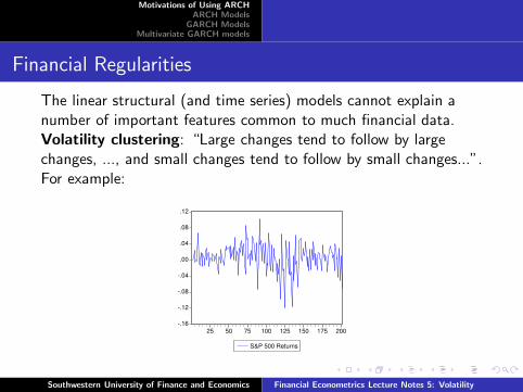
The linear structural (and time series) models cannot explain anumber of important features common to much financial data.Volatility clustering: “Large changes tend to follow by largechanges, ..., and small changes tend to follow by small changes...”.For example:

-.16

-.12

-.08

-.04

.00

.04

.08

.12

25 50 75 100 125 150 175 200

S&P 500 Returns




Financial Regularities Cont’d

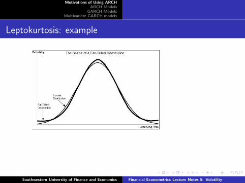
Leptokurtosis: fat tails or thick tails. Kurtosis measures thepeakedness or flatness of the distribution of the series. Kurtosis iscomputed as

K =1

N

N∑

i=1

(

yi − y

σ

)4

(1)

It equals 3 for a normal distribution and above 3 for leptokurtosis,where the distribution is peaked relative to the normal distribution.




Leptokurtosis: example




Financial Regularities Cont’d

Leverage effects: that is changes in stock prices tend to benegatively correlated with changes in volatility, first noted by Black(1976). A firm with debt and equity outstanding typically becomesmore highly leveraged when the value of the firm falls. This raisesequity returns volatility if the returns on the firm as a whole areconstant.

Co-movements in volatilities: volatility changes are not onlyclosely linked across asset within a market, but also across markets.




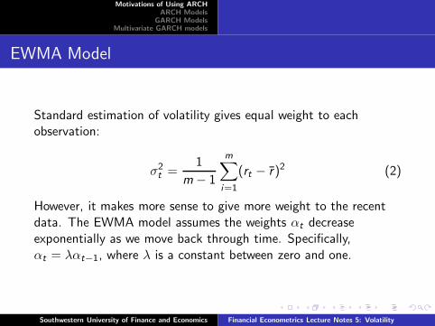
EWMA Model

Standard estimation of volatility gives equal weight to eachobservation:

σ2t =

1

m − 1

m∑

i=1

(rt − r)2 (2)

However, it makes more sense to give more weight to the recentdata. The EWMA model assumes the weights αt decreaseexponentially as we move back through time. Specifically,αt = λαt−1, where λ is a constant between zero and one.




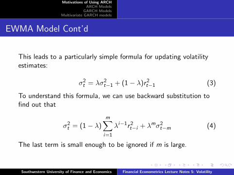
EWMA Model Cont’d

This leads to a particularly simple formula for updating volatilityestimates:

σ2t = λσ2

t−1 + (1 − λ)r2t−1 (3)

To understand this formula, we can use backward substitution tofind out that

σ2t = (1 − λ)

m∑

i=1

λi−1r2t−i + λmσ2

t−m (4)

The last term is small enough to be ignored if m is large.




EWMA Model Cont’d

EWMA is attractive in that only relatively little data is required. Itis designed to track changes in the volatility.

The RiskMetrices database, which was created by J.P. Morgan andmade publicly available in 1994, uses EWMA with λ = 0.94 forupdating daily volatility estimates.




Definition of ARCH ModelsTesting for ARCH Effects

Definition

The autoregressive conditional heteroskedastic (ARCH) class ofmodels was introduced by Engle (1982). Arising from the use ofconditional versus unconditional mean, the key insight offered bythe ARCH model lies in the distinction between conditional andthe unconditional second moments.

While the unconditional covariance matrix for the variables ofinterest may be time invariant, the conditional variances andcovariances often depend non-trivially on the past states of theworld.





Definition Cont’d

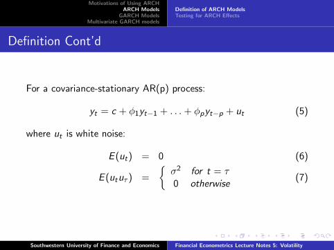
For a covariance-stationary AR(p) process:

yt = c + φ1yt−1 + . . . + φpyt−p + ut (5)

where ut is white noise:

E (ut) = 0 (6)

E (utuτ ) =

{

σ2 for t = τ0 otherwise

(7)





Conditional Vs. Unconditional Mean

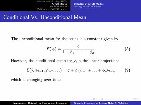
The unconditional mean for the series is a constant given by

E (yt) =c

1 − φ1 − . . . − φp

(8)

However, the conditional mean for yt is the linear projection:

E (yt |yt−1, yt−2, . . .) = c + φ1yt−1 + . . . + φpyt−p (9)

which is changing over time.





ARCH Process

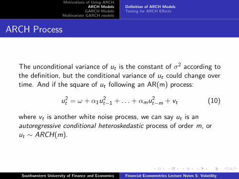
The unconditional variance of ut is the constant of σ2 according tothe definition, but the conditional variance of ut could change overtime. And if the square of ut following an AR(m) process:

u2t = ω + α1u

2t−1 + . . . + αmu2

t−m + vt (10)

where vt is another white noise process, we can say ut is anautoregressive conditional heteroskedastic process of order m, orut ∼ ARCH(m).





Another Way

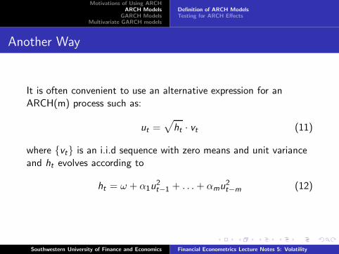
It is often convenient to use an alternative expression for anARCH(m) process such as:

ut =√

ht · vt (11)

where {vt} is an i.i.d sequence with zero means and unit varianceand ht evolves according to

ht = ω + α1u2t−1 + . . . + αmu2

t−m (12)





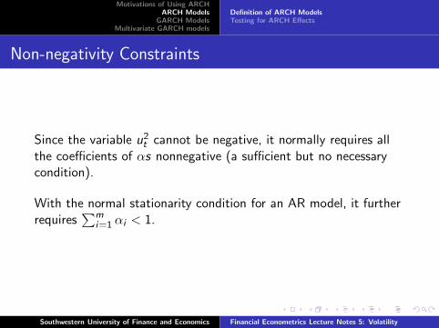
Non-negativity Constraints

Since the variable u2t cannot be negative, it normally requires all

the coefficients of αs nonnegative (a sufficient but no necessarycondition).

With the normal stationarity condition for an AR model, it furtherrequires

∑mi=1 αi < 1.





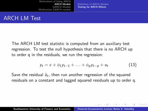
ARCH LM Test

The ARCH LM test statistic is computed from an auxiliary testregression. To test the null hypothesis that there is no ARCH upto order q in the residuals, we run the regression:

yt = c + φ1yt−1 + . . . + φpyt−p + ut (13)

Save the residual ut , then run another regression of the squaredresiduals on a constant and lagged squared residuals up to order q.





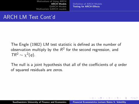
ARCH LM Test Cont’d

The Engle (1982) LM test statistic is defined as the number ofobservation multiply by the R2 for the second regression, andTR2 ∼ χ2(q).

The null is a joint hypothesis that all of the coefficients of q orderof squared residuals are zeros.




the GARCH ModelsEstimation of GARCH ModelsExtensions to GARCH Family

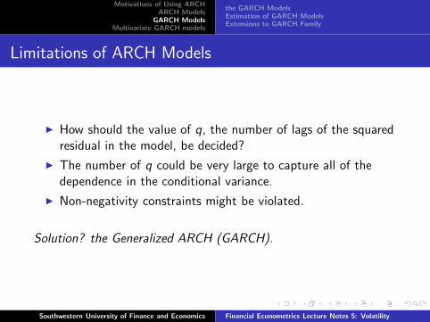
Limitations of ARCH Models

◮ How should the value of q, the number of lags of the squaredresidual in the model, be decided?

◮ The number of q could be very large to capture all of thedependence in the conditional variance.

◮ Non-negativity constraints might be violated.

Solution? the Generalized ARCH (GARCH).





GARCH Model

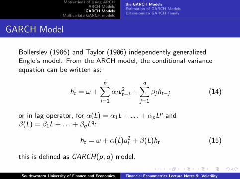
Bollerslev (1986) and Taylor (1986) independently generalizedEngle’s model. From the ARCH model, the conditional varianceequation can be written as:

ht = ω +

p∑

i=1

αiu2t−i +

q∑

j=1

βjht−j (14)

or in lag operator, for α(L) = α1L + . . . + αpLp and

β(L) = β1L + . . . + βqLq:

ht = ω + α(L)u2t + β(L)ht (15)

this is defined as GARCH(p, q) model.





the Benefits of GARCH

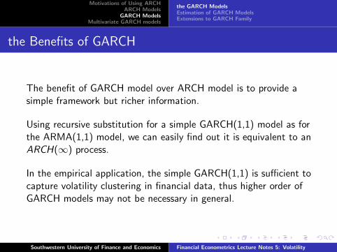
The benefit of GARCH model over ARCH model is to provide asimple framework but richer information.

Using recursive substitution for a simple GARCH(1,1) model as forthe ARMA(1,1) model, we can easily find out it is equivalent to anARCH(∞) process.

In the empirical application, the simple GARCH(1,1) is sufficient tocapture volatility clustering in financial data, thus higher order ofGARCH models may not be necessary in general.





Recursive Substitution

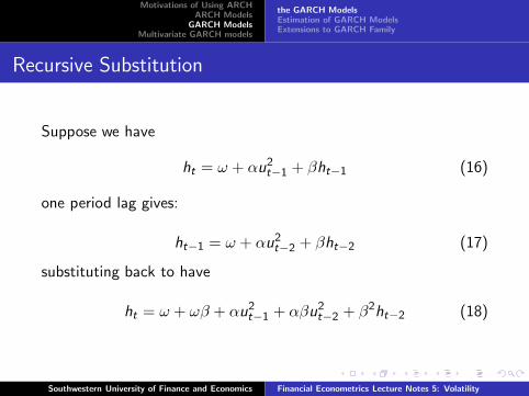
Suppose we have

ht = ω + αu2t−1 + βht−1 (16)

one period lag gives:

ht−1 = ω + αu2t−2 + βht−2 (17)

substituting back to have

ht = ω + ωβ + αu2t−1 + αβu2

t−2 + β2ht−2 (18)





Recursive Substitution Cont’d

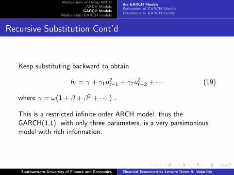
Keep substituting backward to obtain

ht = γ + γ1u2t−1 + γ2u

2t−2 + · · · (19)

where γ = ω(1 + β + β2 + · · · ) .

This is a restricted infinite order ARCH model, thus theGARCH(1,1), with only three parameters, is a very parsimoniousmodel with rich information.





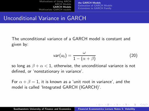
Unconditional Variance in GARCH

The unconditional variance of a GARCH model is constant andgiven by:

var(ut) =ω

1 − (α + β)(20)

so long as β + α < 1, otherwise, the unconditional variance is notdefined, or ‘nonstationary in variance’.

For α + β = 1, it is known as a ‘unit root in variance’, and themodel is called ‘Integrated GARCH (IGARCH)’.





Estimation of GARCH Models

◮ Since the model is no longer of the usual linear form, wecannot use OLS.

◮ Another technique known as maximum likelihood is employed.

◮ The method works by finding the most likely values of theparameters given the actual data.

◮ More specifically, a log-likelihood function is formed and thevalues of the parameters that maximise it are sought.





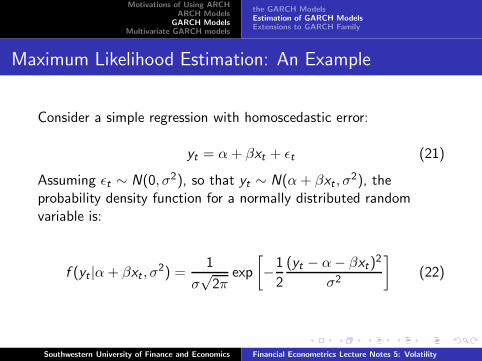
Maximum Likelihood Estimation: An Example

Consider a simple regression with homoscedastic error:

yt = α + βxt + ǫt (21)

Assuming ǫt ∼ N(0, σ2), so that yt ∼ N(α + βxt , σ2), the

probability density function for a normally distributed randomvariable is:

f (yt |α + βxt , σ2) =

1

σ√

2πexp

[

−1

2

(yt − α − βxt)2

σ2

]

(22)





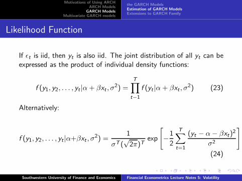
Likelihood Function

If ǫt is iid, then yt is also iid. The joint distribution of all yt can beexpressed as the product of individual density functions:

f (y1, y2, . . . , yt |α + βxt , σ2) =

T∏

t−1

f (yt |α + βxt , σ2) (23)

Alternatively:

f (y1, y2, . . . , yt |α+βxt , σ2) =

1

σT (√

2π)Texp

[

−1

2

T∑

t=1


σ2

]

(24)





Log Likelihood Function

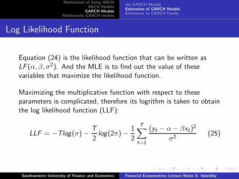
Equation (24) is the likelihood function that can be written asLF (α, β, σ2). And the MLE is to find out the value of thesevariables that maximize the likelihood function.

Maximizing the multiplicative function with respect to theseparameters is complicated, therefore its logrithm is taken to obtainthe log likelihood function (LLF):

LLF = −Tlog(σ) − T

2log(2π) − 1

2

T∑

t=1


σ2(25)





Maximum Likelihood Estimation: solution

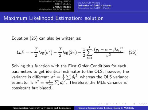
Equation (25) can also be written as:

LLF = −T

2log(σ2) − T

2log(2π) − 1

2

T∑

t=1


σ2(26)

Solving this function with the First Order Conditions for eachparameters to get identical estimator to the OLS, however, thevariance is different: σ2 = 1

T

∑

ut2, whereas the OLS variance

estimator is σ2 = 1T−k

∑

ut2. Therefore, the MLE variance is

consistant but biased.





Estimate GARCH Model with MLE

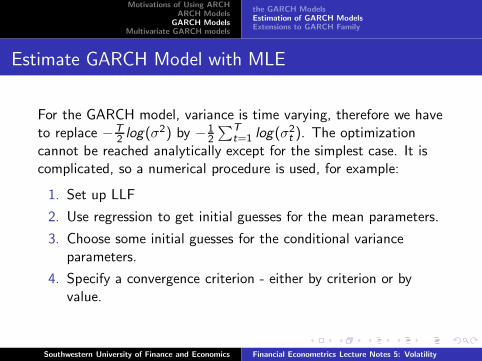
For the GARCH model, variance is time varying, therefore we haveto replace −T

2 log(σ2) by −12

∑Tt=1 log(σ2

t ). The optimizationcannot be reached analytically except for the simplest case. It iscomplicated, so a numerical procedure is used, for example:

1. Set up LLF

2. Use regression to get initial guesses for the mean parameters.

3. Choose some initial guesses for the conditional varianceparameters.

4. Specify a convergence criterion - either by criterion or byvalue.





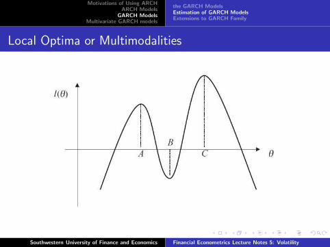
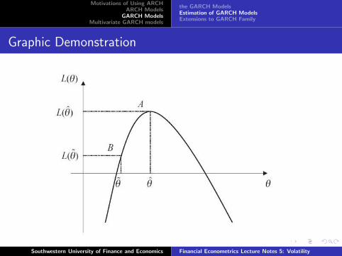
Local Optima or Multimodalities





the ‘Trinity’ of tests

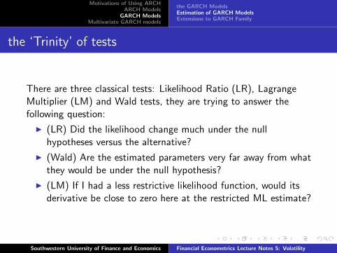
There are three classical tests: Likelihood Ratio (LR), LagrangeMultiplier (LM) and Wald tests, they are trying to answer thefollowing question:

◮ (LR) Did the likelihood change much under the nullhypotheses versus the alternative?

◮ (Wald) Are the estimated parameters very far away from whatthey would be under the null hypothesis?

◮ (LM) If I had a less restrictive likelihood function, would itsderivative be close to zero here at the restricted ML estimate?





Likelihood Ratio Test

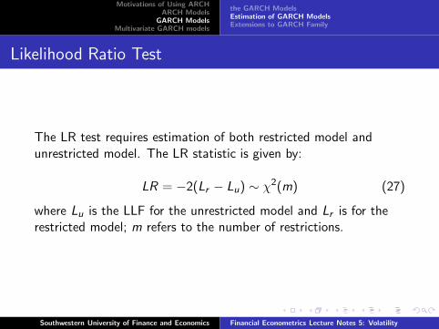
The LR test requires estimation of both restricted model andunrestricted model. The LR statistic is given by:

LR = −2(Lr − Lu) ∼ χ2(m) (27)

where Lu is the LLF for the unrestricted model and Lr is for therestricted model; m refers to the number of restrictions.





Lagrange Multiplier Test

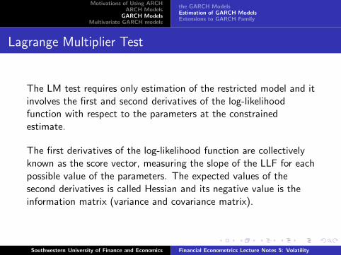
The LM test requires only estimation of the restricted model and itinvolves the first and second derivatives of the log-likelihoodfunction with respect to the parameters at the constrainedestimate.

The first derivatives of the log-likelihood function are collectivelyknown as the score vector, measuring the slope of the LLF for eachpossible value of the parameters. The expected values of thesecond derivatives is called Hessian and its negative value is theinformation matrix (variance and covariance matrix).





Wald Test

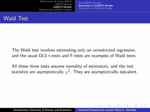
The Wald test involves estimating only an unrestricted regression,and the usual OLS t-tests and F-tests are examples of Wald tests.

All these three tests assume nomality of estimators, and the teststatistics are asymptotically χ2. They are asymptotically eqivalent.





Graphic Demonstration





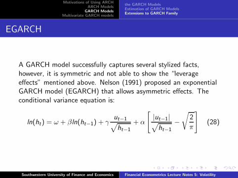
EGARCH

A GARCH model successfully captures several stylized facts,however, it is symmetric and not able to show the “leverageeffects” mentioned above. Nelson (1991) proposed an exponentialGARCH model (EGARCH) that allows asymmetric effects. Theconditional variance equation is:

ln(ht) = ω + βln(ht−1) + γut−1

√

ht−1

+ α

[

|ut−1|√

ht−1

−√

2

π

]

(28)





EGARCH cont’d

The benefits of such parameterizations is no need for furthernonnegative restrictions for the parameters since nature logarithmis been applied, furthermore, if there is indeed asymmetric effectswhere negative shock cause larger volatility, γ will be negative.

An additional notes about EGARCH is that Nelson (1991)proposed using the Generalized error distribution (GED)normalized to have zero mean and unit variance rather thannormal distribution for the ML estimation.





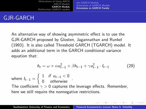
GJR-GARCH

An alternative way of showing asymmetric effect is to use theGJR-GARCH proposed by Glosten, Jagannathan and Runkel(1993). It is also called Threshold GARCH (TGARCH) model. Itadds an additional term in the GARCH conditional varianceequation that:

ht = ω + αu2t−1 + βht−1 + γu2

t−1 · It−1 (29)

where It−1 =

{

1 if ut−1 < 00 otherwise

.

The coefficient γ > 0 captures the leverage effects. Remember,here we still require the nonnegative restrictions.





Tests for Asymmtries

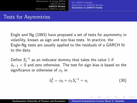
Engle and Ng (1993) have proposed a set of tests for asymmetry involatility, known as sign and size bias tests. In practice, theEngle-Ng tests are usually applied to the residuals of a GARCH fitto the data.

Define S−1t as an indicator dummy that takes the value 1 if

ut−1 < 0 and zero otherwise. The test for sign bias is based on thesignificance or otherwise of φ1 in

u2t = φ0 + φ1S

−1t + vt (30)





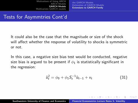
Tests for Asymmtries Cont’d

It could also be the case that the magnitude or size of the shockwill affect whether the response of volatility to shocks is symmetricor not.

In this case, a negative size bias test would be conducted, negativesize bias is argued to be present if φ1 is statistically significant inthe regression:

u2t = φ0 + φ1S

−1t ut−1 + vt (31)





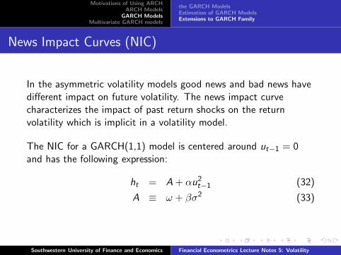
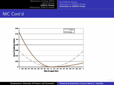
News Impact Curves (NIC)

In the asymmetric volatility models good news and bad news havedifferent impact on future volatility. The news impact curvecharacterizes the impact of past return shocks on the returnvolatility which is implicit in a volatility model.

The NIC for a GARCH(1,1) model is centered around ut−1 = 0and has the following expression:

ht = A + αu2t−1 (32)

A ≡ ω + βσ2 (33)





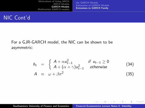
NIC Cont’d

For a GJR-GARCH model, the NIC can be shown to beasymmetric:

ht =

{

A + αu2t−1 if ut−1 ≥ 0

A + (α + γ)u2t−1 otherwise

(34)

A ≡ ω + βσ2 (35)





NIC Cont’d





GARCH in Mean

It is normally agreed that an asset with a higher risk would pay ahigher return. The conditional covariance with an appropriatelydefined benchmark portfolio often serves to price the assets.

For example, according to the traditional capital asset pricingmodel (CAPM) the excess returns on all risky assets areproportional to the non-diversifiable risk as measured by thecovariances with the market portfolio.





GARCH in Mean Cont’d

The GARCH in mean (GARCH-M) model proposed by Engle,Lilien and Robins (1987) are defined as:

yt = µ + δg(ht−1) + ut (36)

ht = ω + αu2t−1 + βht−1 (37)

where g(·) is a function of conditional variance, which can be thelevel, the square roots or natural logarithm.




Covariance and CorrelationApplication: Dynamic Hedge Ratio

Estimate Covariance and Correlation

Covariance or correlation between two series can be calculated inthe standard way using a set of historical data.

It can also be estimated using EWMA specificaiton:

σ(x , y)t = (1 − λ)

m∑

i=0

λixt−iyt−i (38)

Multivariate GARCH models are used to estimate and to forecastcovariances and correlations to allow for the time-varying nature.





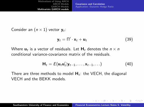
Consider an (n × 1) vector yt :

yt = Π′ · xt + ut (39)

Where ut is a vector of residuals. Let Ht denotes the n × nconditional variance-covariance matrix of the residuals.

Ht = E (utu′

t |yt−1, . . . , xt−1, . . .) (40)

There are three methods to model Ht : the VECH, the diagonalVECH and the BEKK models.





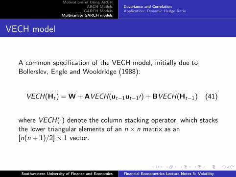
VECH model

A common specification of the VECH model, initially due toBollerslev, Engle and Wooldridge (1988):

VECH(Ht) = W + AVECH(ut−1ut−1′) + BVECH(Ht−1) (41)

where VECH(·) denote the column stacking operator, which stacksthe lower triangular elements of an n × n matrix as an[n(n + 1)/2] × 1 vector.





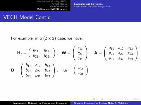
VECH Model Cont’d

For example, in a (2 × 2) case, we have:

Ht =

(

h11t h12t

h21t h22t

)

, W =

c11

c21

c31

, A =

a11 a12 a13

a21 a22 a23

a31 a32 a33

B =

b11 b12 b13

b21 b22 b23

b31 b32 b33

, ut =

(

u1t

u2t

)





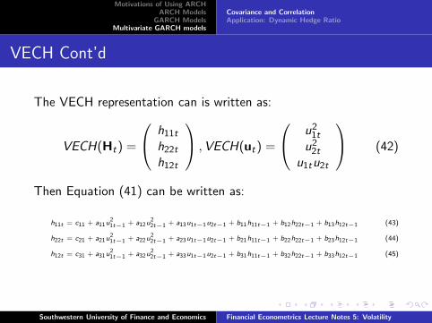
VECH Cont’d

The VECH representation can is written as:

VECH(Ht) =

h11t

h22t

h12t

,VECH(ut) =

u21t

u22t

u1tu2t

(42)

Then Equation (41) can be written as:

h11t = c11 + a11u21t−1 + a12u

22t−1 + a13u1t−1u2t−1 + b11h11t−1 + b12h22t−1 + b13h12t−1 (43)

h22t = c21 + a21u21t−1 + a22u


h12t = c31 + a31u21t−1 + a32u






Diagonal VECH

Bollerslev et al. (1988) suggest that the coefficient matrix A andB to be diagonal. Which means the (i , j)th elements of Ht onlydepend on the corresponding (i , j)th elements of Ht−1 andut−1u

′

t−1.

Diagonal VECH model does not allow for causality in variance,co-persistence in variance, or asymmetries. Furthermore, the modelmay not guarantee a positive definite conditional covariance matrix.





BEKK Model

An alternative model proposed by Engle and Kroner (1995) is theBEKK model that have:

Ht = V′V + A′Ht−1A + B′ut−1ut−1B (46)

which guaranteed for the conditional covariance matrix to bepositive definite due to the quadratic nature of the terms on theRHS of equations.





Hedging

The simplest and perhaps the most widely used method forreducing and managing risk is hedging with futures contracts.

A hedge is achieved by taking opposite positions in spot andfutures markets simultaneously, so that any loss sustained from anadverse price movement in one market should to some degree beoffset by a favourable price movement in the other.





Hedge Ratio

The ratio of the number of units of the futures asset that arepurchased relative to the number of units of the spot asset isknown as the hedge ratio.

The optimal hedge ratio is to choose a ratio which minimises thevariance of the returns of a portfolio containing the spot andfutures position.





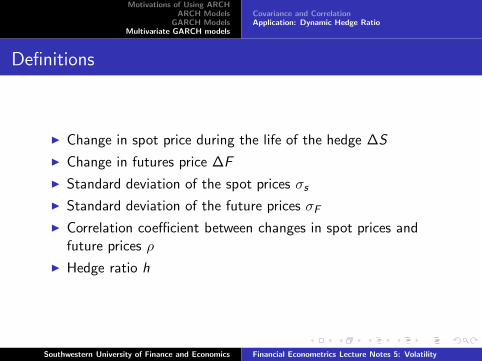
Definitions

◮ Change in spot price during the life of the hedge ∆S

◮ Change in futures price ∆F

◮ Standard deviation of the spot prices σs

◮ Standard deviation of the future prices σF

◮ Correlation coefficient between changes in spot prices andfuture prices ρ

◮ Hedge ratio h





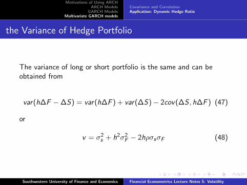
the Variance of Hedge Portfolio

The variance of long or short portfolio is the same and can beobtained from

var(h∆F − ∆S) = var(h∆F ) + var(∆S) − 2cov(∆S , h∆F ) (47)

or

v = σ2s + h2σ2

F − 2hρσsσF (48)





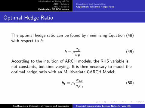
Optimal Hedge Ratio

The optimal hedge ratio can be found by minimizing Equation (48)with respect to h:

h = ρσs

σF

(49)

According to the intuition of ARCH models, the RHS variable isnot constants, but time-varying. It is then necessary to model theoptimal hedge ratio with an Multivariate GARCH Model:

ht = ρt

σs,t

σF ,t

(50)





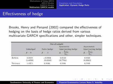
Effectiveness of hedge

Brooks, Henry and Persand (2002) compared the effectiveness ofhedging on the basis of hedge ratios derived from variousmultivariate GARCH specifications and other, simpler techniques.


Documents

Financial Econometrics Lecture 5: Modelling Volatility and ... · Financial Econometrics Lecture 5: Modelling Volatility and Correlation Dayong Zhang Research Institute of Economics