Embed Size (px)
Citation preview
Johnson, et al. Supporting Information
S1
Supporting Information for:
Continuous Liquid Vapor Reactions Part 1: Design and Characterization of a Reactor for
Asymmetric Hydroformylation
Martin D. Johnson,†,* Scott A. May,
† Joel R. Calvin,
† Gordon R. Lambertus,
† Prashant B. Kokitkar
† Clark R.
Landis‡, Bradley R. Jones
‡, Leigh Abrams
‡, James R. Stout
#
†Small Molecule Design and Development, Eli Lilly and Company, Indianapolis, Indiana 46285, Unites States
‡ Department of Chemistry, University of Wisconsin—Madison, 1101 University Avenue, Madison Wisconsin 53706, United States
#D&M Continuous Solutions, LLC, Greenwood, IN 46143, United States
1. Measurement of vapor/liquid mass transfer rates in small diameter tubing..................................................... 2
2.Quantifying axial dispersion and mean residence time in continuous reactor via nonreactive solvent tracer
runs ................................................................................................................................................................. 6
3.Reactor modeling and quantifying rate constants. ........................................................................................ 12
4. Pressure and gas flow control in second and third generation continuous reactors. ....................................... 14
5. Custom automated sampling/dilution/parking system used for On-line HPLC. ............................................ 22
Johnson, et al. Supporting Information
S2
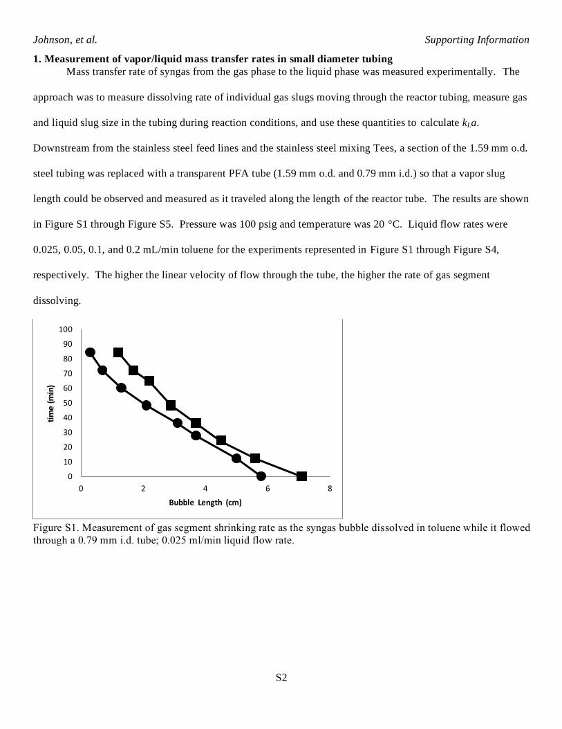
1. Measurement of vapor/liquid mass transfer rates in small diameter tubing
Mass transfer rate of syngas from the gas phase to the liquid phase was measured experimentally. The
approach was to measure dissolving rate of individual gas slugs moving through the reactor tubing, measure gas
and liquid slug size in the tubing during reaction conditions, and use these quantities to calculate kLa.
Downstream from the stainless steel feed lines and the stainless steel mixing Tees, a section of the 1.59 mm o.d.
steel tubing was replaced with a transparent PFA tube (1.59 mm o.d. and 0.79 mm i.d.) so that a vapor slug
length could be observed and measured as it traveled along the length of the reactor tube. The results are shown
in Figure S1 through Figure S5. Pressure was 100 psig and temperature was 20 °C. Liquid flow rates were
0.025, 0.05, 0.1, and 0.2 mL/min toluene for the experiments represented in Figure S1 through Figure S4,
respectively. The higher the linear velocity of flow through the tube, the higher the rate of gas segment
dissolving.
Figure S1. Measurement of gas segment shrinking rate as the syngas bubble dissolved in toluene while it flowed
through a 0.79 mm i.d. tube; 0.025 ml/min liquid flow rate.
0
10
20
30
40
50
60
70
80
90
100
0 2 4 6 8
tim
e (m
in)
Bubble Length (cm)
Johnson, et al. Supporting Information
S3
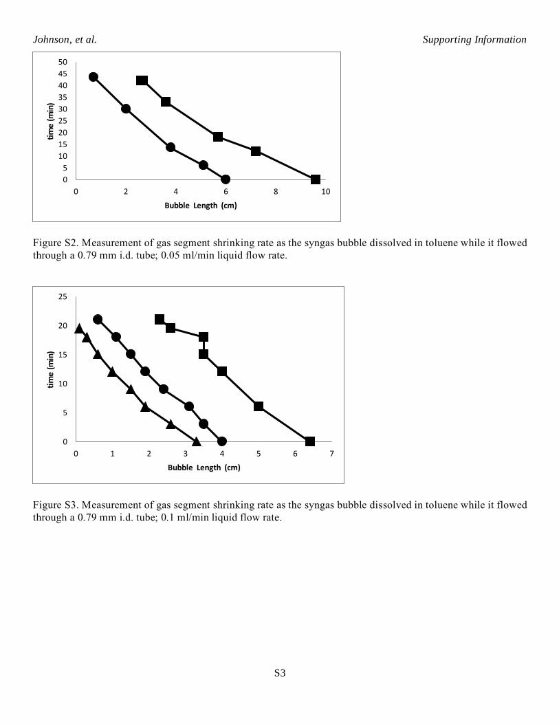
Figure S2. Measurement of gas segment shrinking rate as the syngas bubble dissolved in toluene while it flowed
through a 0.79 mm i.d. tube; 0.05 ml/min liquid flow rate.
Figure S3. Measurement of gas segment shrinking rate as the syngas bubble dissolved in toluene while it flowed
through a 0.79 mm i.d. tube; 0.1 ml/min liquid flow rate.
0
5
10
15
20
25
30
35
40
45
50
0 2 4 6 8 10
tim
e (m
in)
Bubble Length (cm)
0
5
10
15
20
25
0 1 2 3 4 5 6 7
tim
e (m
in)
Bubble Length (cm)
Johnson, et al. Supporting Information
S4
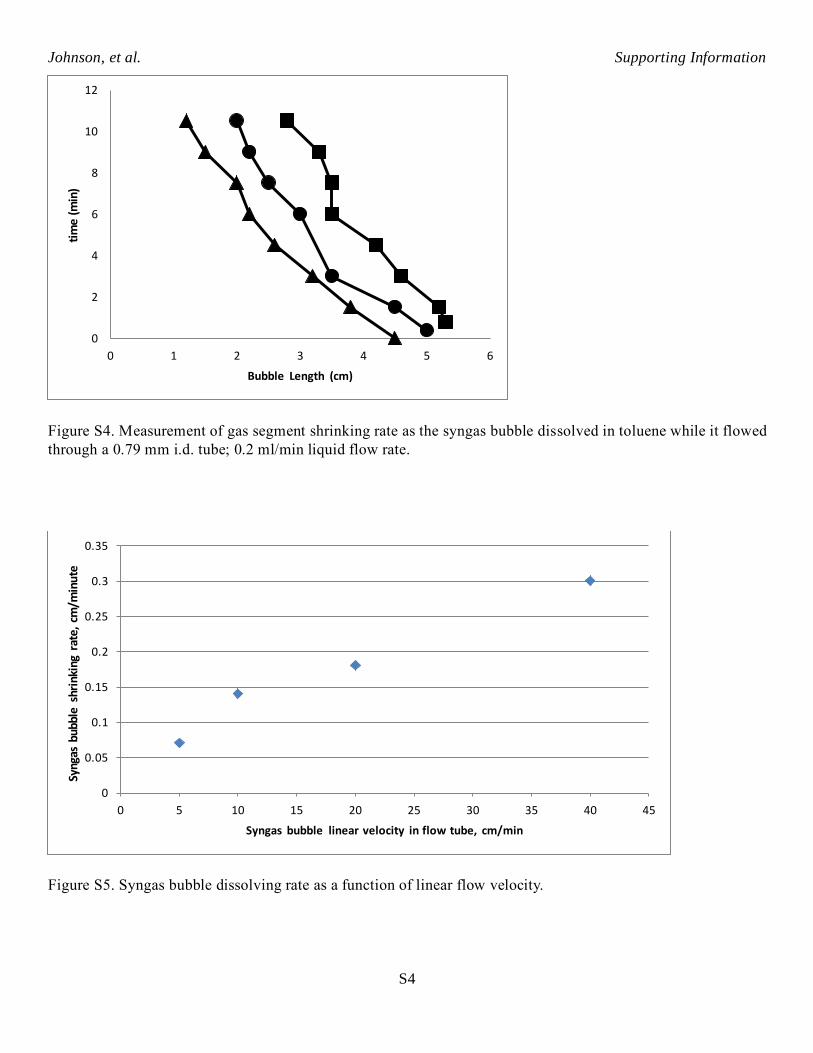
Figure S4. Measurement of gas segment shrinking rate as the syngas bubble dissolved in toluene while it flowed
through a 0.79 mm i.d. tube; 0.2 ml/min liquid flow rate.
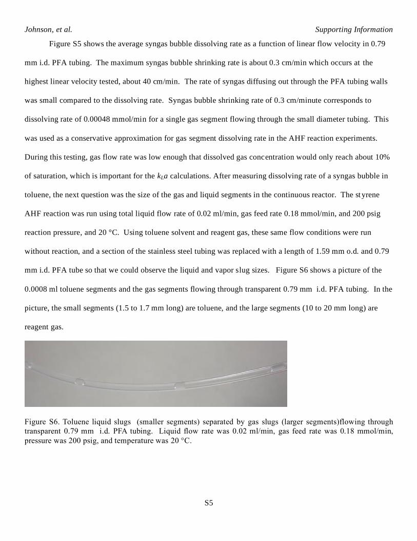
Figure S5. Syngas bubble dissolving rate as a function of linear flow velocity.
0
2
4
6
8
10
12
0 1 2 3 4 5 6
tim
e (m
in)
Bubble Length (cm)
0
0.05
0.1
0.15
0.2
0.25
0.3
0.35
0 5 10 15 20 25 30 35 40 45
Syng
as b
ubbl
e sh
rink
ing
rate
, cm
/min
ute
Syngas bubble linear velocity in flow tube, cm/min
Johnson, et al. Supporting Information
S5
Figure S5 shows the average syngas bubble dissolving rate as a function of linear flow velocity in 0.79
mm i.d. PFA tubing. The maximum syngas bubble shrinking rate is about 0.3 cm/min which occurs at the
highest linear velocity tested, about 40 cm/min. The rate of syngas diffusing out through the PFA tubing walls
was small compared to the dissolving rate. Syngas bubble shrinking rate of 0.3 cm/minute corresponds to
dissolving rate of 0.00048 mmol/min for a single gas segment flowing through the small diameter tubing. This
was used as a conservative approximation for gas segment dissolving rate in the AHF reaction experiments.
During this testing, gas flow rate was low enough that dissolved gas concentration would only reach about 10%
of saturation, which is important for the kLa calculations. After measuring dissolving rate of a syngas bubble in
toluene, the next question was the size of the gas and liquid segments in the continuous reactor. The styrene
AHF reaction was run using total liquid flow rate of 0.02 ml/min, gas feed rate 0.18 mmol/min, and 200 psig
reaction pressure, and 20 °C. Using toluene solvent and reagent gas, these same flow conditions were run
without reaction, and a section of the stainless steel tubing was replaced with a length of 1.59 mm o.d. and 0.79
mm i.d. PFA tube so that we could observe the liquid and vapor slug sizes. Figure S6 shows a picture of the
0.0008 ml toluene segments and the gas segments flowing through transparent 0.79 mm i.d. PFA tubing. In the
picture, the small segments (1.5 to 1.7 mm long) are toluene, and the large segments (10 to 20 mm long) are
reagent gas.
Figure S6. Toluene liquid slugs (smaller segments) separated by gas slugs (larger segments)flowing through
transparent 0.79 mm i.d. PFA tubing. Liquid flow rate was 0.02 ml/min, gas feed rate was 0.18 mmol/min,
pressure was 200 psig, and temperature was 20 °C.
Johnson, et al. Supporting Information
S6
The measured gas dissolving rate and liquid slug size were used to calculate kLa, as shown in Table S1.
The first row in the table lists the conservative estimate for gas slug dissolving rate to reach 10% of saturation,
0.00048 mmol/min for each individual gas slug. At reaction conditions, gas dissolving rate for each vapor slug
would actually be higher, because linear velocity in the tubing was 4X higher, pressure was 2X higher, and
temperature was 50 °C higher for the reaction compared to the bubble dissolving rate test. Therefore kLa = 0.1
s-1
is a low estimate.
Table S1. Calculation of kLa in 0.56 mm i.d. tube.
Conservative estimated of gas slug dissolving rate for each individual bubble,
until liquid reaches 10% of saturation 0.00048 mmol/min
Liquid slug volume 0.0008 ml
Total liquid volumetric feed rate liquid 0.02 ml/min
pressure 200 psig
gas feed rate 0.18 mmol/min
linear velocity in 0.56 mm i.d. tubing at mixing Tee 150-160 cm/min
predicted saturated gas concentration 0.09 mmol/ml
calculated time to 10% of saturation 0.9 second
Calculated kLa 0.11 sec-1
2.Quantifying axial dispersion and mean residence time in continuous reactor via nonreactive solvent
tracer runs
Real reactors are not ideal and do not have ideal plug flow behavior. Dispersion in the axial direction
causes some fluid elements to travel through the reactor faster than others. Axial dispersion must be quantified
so that it can be used in the non-ideal reactor models to calculate time to a given %conversion. If we know
axial dispersion and reaction kinetics for a positive order reaction, then this information is used to quantify how
much more time will be required for a given % conversion in a real flow reactor compared to an ideal PFR or a
batch reactor. Alternatively, if we know axial dispersion and we measure conversion versus distance in a
continuous reactor, then we can use the information to model the reactor numerically and calculate the real
reaction rate constants, which was done in this study.
Levenspiel showed that the vessel dispersion number (D/uL) can be used to quantify the extent of
dispersion in a given vessel under a set of operating conditions, where D is the Taylor longitudinal dispersion
Johnson, et al. Supporting Information
S7
coefficient that incorporates the effect of both diffusion and convection, u is average flow velocity and L is
vessel lengthi. As axial dispersion increases, so does the reaction time required for a given conversion. Plotting
C/Cf versus t/τ after a step change in non-reactive tracer flowing into a tube produces an s-shaped curve (for
example see Figure S7), where C is nonreactive tracer concentration at exit and Cf is tracer concentration once
steady state is achieved after the change. Dankwerts defined this as the F-curve.ii These transition curves were
measured experimentally and the data was modeled by two methods: The plug flow with dispersion reactor
(PFDR) method and the CSTRs in series method.
Using the PFDR model, D/uL can be calculated by fitting experimental F-curve data to the basic
differential equation representing dispersion by numerically solving for D/uL and θ as shown in the following
equation:
𝜕𝐶
𝜕𝜃= (
𝑫
𝑢𝐿)𝜕2𝐶
𝜕𝑧2−𝜕𝐶
𝜕𝑧
D/uL = vessel dispersion number
θ = dimensionless time (t/τ)
Z = dimensionless length (x/L)
See chemical engineering textbooks for details on the methods and analysesiii
. For small extents of dispersion,
D/uL < 0.01, the equation can be solved analytically to give the following symmetrical C-curve:
𝐶 =1
2√𝜋(𝑫
𝑢𝐿)
exp[−(1 − 𝜃)2
4(𝑫
𝑢𝐿)
]
This equation was used to quantify D/uL and θ for the experimental F-curves. The experimental F-curve data
was also fit to the CSTRs-in-series reactor model. Theoretically an ideal PFR is the same as an infinite number
of CSTRs in series each with infinitesimally small volume. A PFDR with axial dispersion number about 0.015
has about the same residence time distribution (RTD) as 36 equal volume CSTRs in series. The process fluid
volume in each theoretical CSTR unit is total reactor volume divided by 36. The E-curve represents the spread
of non-reactive tracer as it moves along the reactor. The E-curve of CSTRs in series is mathematically equal
toiv
:
Johnson, et al. Supporting Information
S8
𝐸(𝑡) =𝑒−𝑡/𝜏
𝜏(𝑛 − 1)!(𝑛𝑡
𝜏)𝑛−1
Where n = number of CSTRs in series of equal .
The F-curve can be generated because it is the time integral of the E-curve:
𝐹(𝑡) = ∫ 𝐸(𝑡)𝑑𝑡𝑡
0
For each axial dispersion experiment, the F-curve was obtained by making a step change from THF + toluene to
THF + xylenes flowing into the tube, or vice versa, and monitoring the concentration of toluene and xylenes in
the reactor effluent. Samples were collected by an on-line auto-sampler described in the experimental section.
When measuring F-curves in this manner it is important to note that the curve may change shape by more than
5% while it is being measured if D/uL > 0.01. The experimental F-curves along with PFDR and CSTRs-in-
series model fits are show in Figure S7 through Figure S14. The CSTRs in series model fit the RTD profile
better than the PFDR model. This is not surprising given that each of the 20 vertical pipes was well -mixed by
the gas bubbling and likely had the RTD of a CSTR, and the vertical pipe “CSTRs” dominated the RTD. Model
fit showed greater than the equivalent of 20 CSTRs in series, which is not surprising because the reactor was
actually composed of 20 CSTRs separated by 20 PFRs.
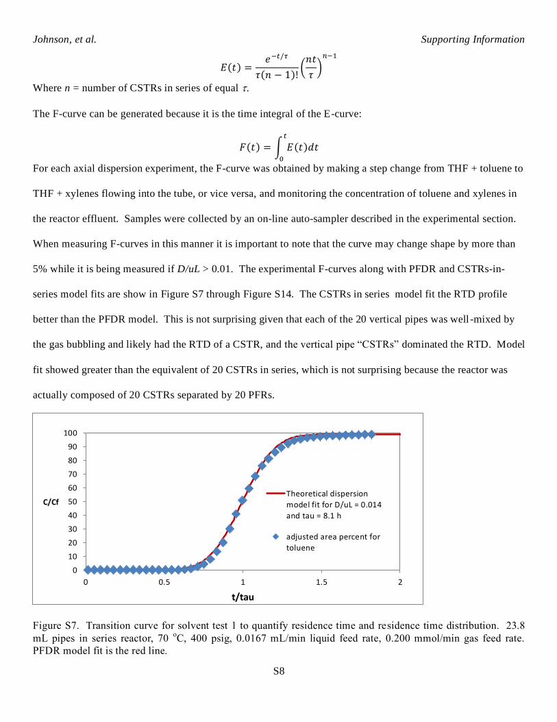
Figure S7. Transition curve for solvent test 1 to quantify residence time and residence time distribution. 23.8
mL pipes in series reactor, 70 oC, 400 psig, 0.0167 mL/min liquid feed rate, 0.200 mmol/min gas feed rate.
PFDR model fit is the red line.
0
10
20
30
40
50
60
70
80
90
100
0 0.5 1 1.5 2
C/Cf
t/tau
Theoretical dispersion
model fit for D/uL = 0.014
and tau = 8.1 h
adjusted area percent for
toluene
Johnson, et al. Supporting Information
S9
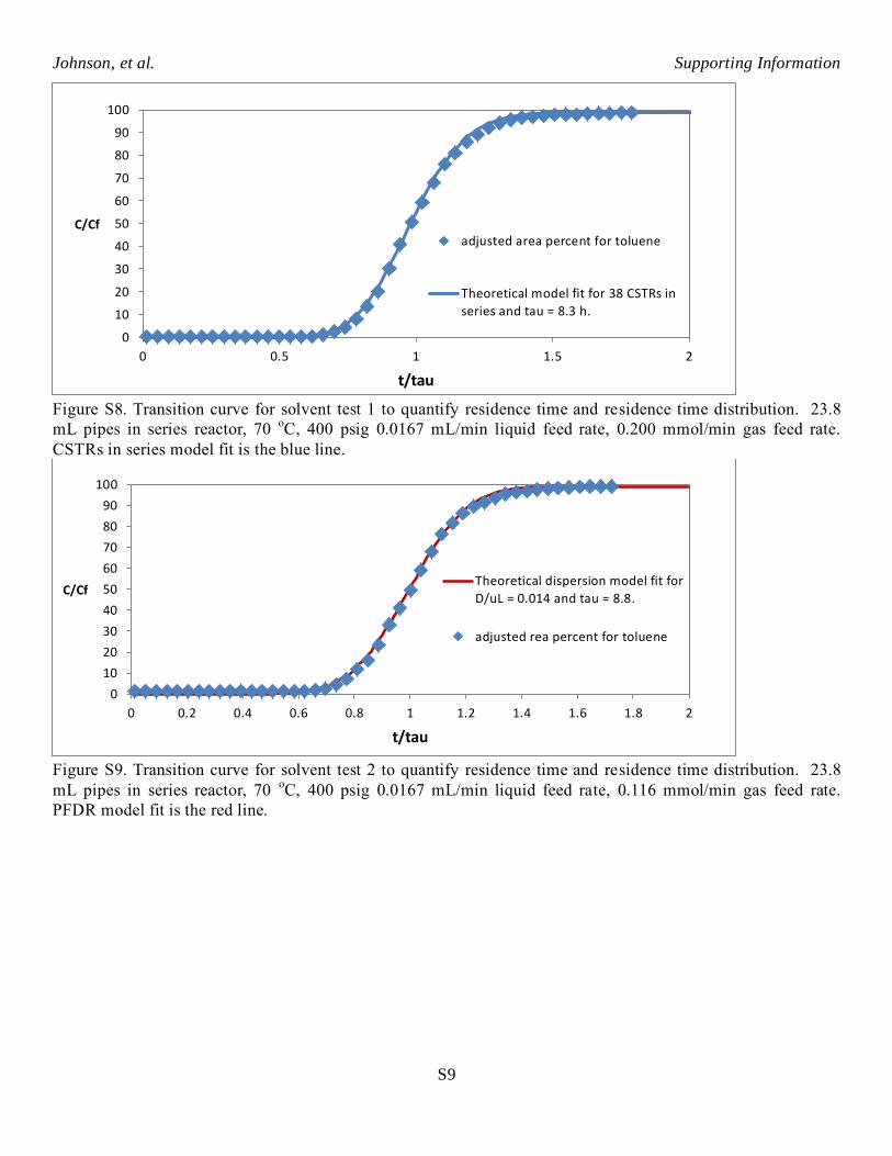
Figure S8. Transition curve for solvent test 1 to quantify residence time and residence time distribution. 23.8
mL pipes in series reactor, 70 oC, 400 psig 0.0167 mL/min liquid feed rate, 0.200 mmol/min gas feed rate.
CSTRs in series model fit is the blue line.
Figure S9. Transition curve for solvent test 2 to quantify residence time and residence time distribution. 23.8
mL pipes in series reactor, 70 oC, 400 psig 0.0167 mL/min liquid feed rate, 0.116 mmol/min gas feed rate.
PFDR model fit is the red line.
0
10
20
30
40
50
60
70
80
90
100
0 0.5 1 1.5 2
C/Cf
t/tau
adjusted area percent for toluene
Theoretical model fit for 38 CSTRs in
series and tau = 8.3 h.
0
10
20
30
40
50
60
70
80
90
100
0 0.2 0.4 0.6 0.8 1 1.2 1.4 1.6 1.8 2
C/Cf
t/tau
Theoretical dispersion model fit for
D/uL = 0.014 and tau = 8.8.
adjusted rea percent for toluene
Johnson, et al. Supporting Information
S10
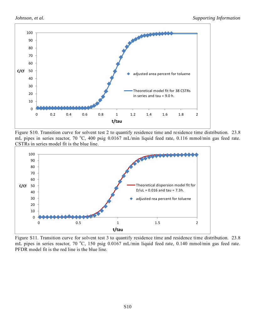
Figure S10. Transition curve for solvent test 2 to quantify residence time and residence time distribution. 23.8
mL pipes in series reactor, 70 oC, 400 psig 0.0167 mL/min liquid feed rate, 0.116 mmol/min gas feed rate.
CSTRs in series model fit is the blue line.
Figure S11. Transition curve for solvent test 3 to quantify residence time and residence time distribution. 23.8
mL pipes in series reactor, 70 oC, 150 psig 0.0167 mL/min liquid feed rate, 0.140 mmol/min gas feed rate.
PFDR model fit is the red line is the blue line.
0
10
20
30
40
50
60
70
80
90
100
0 0.2 0.4 0.6 0.8 1 1.2 1.4 1.6 1.8 2
C/Cf
t/tau
adjusted area percent for toluene
Theoretical model fit for 38 CSTRs
in series and tau = 9.0 h.
0
10
20
30
40
50
60
70
80
90
100
0 0.5 1 1.5 2
C/Cf
t/tau
Theoretical dispersion model fit for
D/uL = 0.016 and tau = 7.3h.
adjusted rea percent for toluene
Johnson, et al. Supporting Information
S11
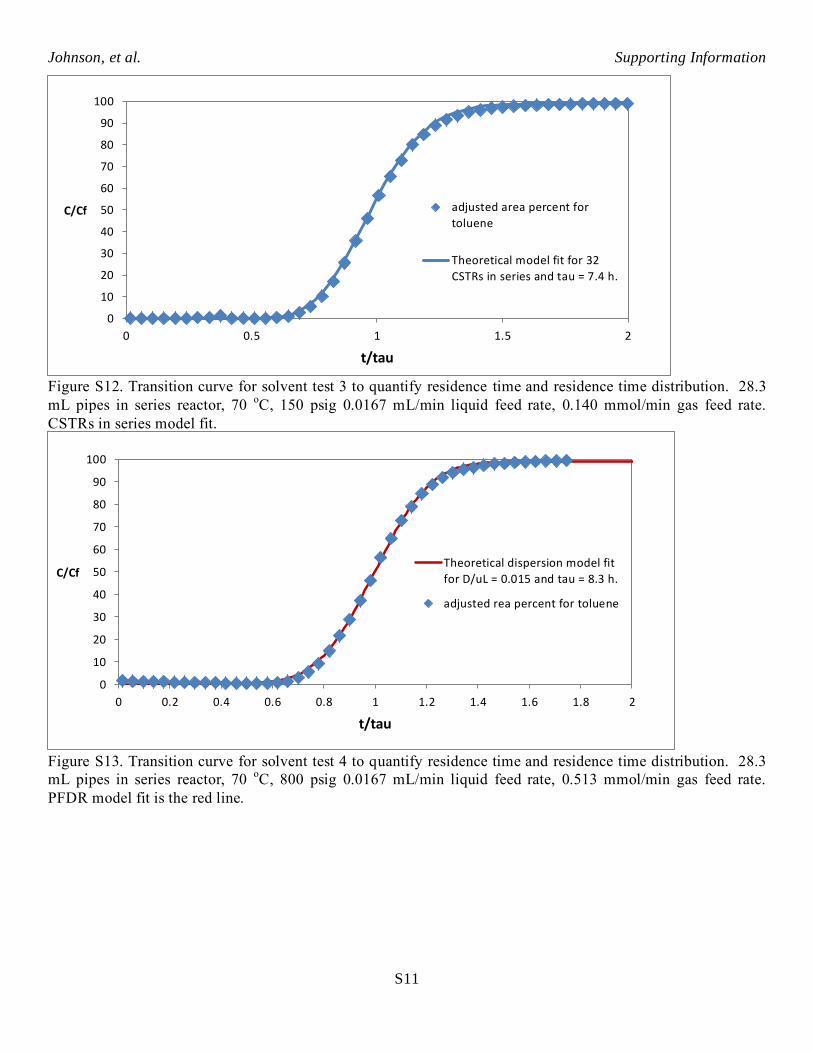
Figure S12. Transition curve for solvent test 3 to quantify residence time and residence time distribution. 28.3
mL pipes in series reactor, 70 oC, 150 psig 0.0167 mL/min liquid feed rate, 0.140 mmol/min gas feed rate.
CSTRs in series model fit.
Figure S13. Transition curve for solvent test 4 to quantify residence time and residence time distribution. 28.3
mL pipes in series reactor, 70 oC, 800 psig 0.0167 mL/min liquid feed rate, 0.513 mmol/min gas feed rate.
PFDR model fit is the red line.
0
10
20
30
40
50
60
70
80
90
100
0 0.5 1 1.5 2
C/Cf
t/tau
adjusted area percent for
toluene
Theoretical model fit for 32
CSTRs in series and tau = 7.4 h.
0
10
20
30
40
50
60
70
80
90
100
0 0.2 0.4 0.6 0.8 1 1.2 1.4 1.6 1.8 2
C/Cf
t/tau
Theoretical dispersion model fit
for D/uL = 0.015 and tau = 8.3 h.
adjusted rea percent for toluene
Johnson, et al. Supporting Information
S12
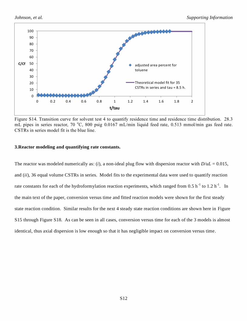
Figure S14. Transition curve for solvent test 4 to quantify residence time and residence time distribution. 28.3
mL pipes in series reactor, 70 oC, 800 psig 0.0167 mL/min liquid feed rate, 0.513 mmol/min gas feed rate.
CSTRs in series model fit is the blue line.
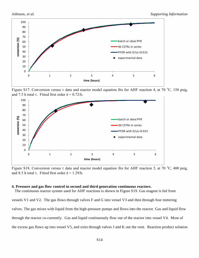
3.Reactor modeling and quantifying rate constants.
The reactor was modeled numerically as: (i), a non-ideal plug flow with dispersion reactor with D/uL = 0.015,
and (ii), 36 equal volume CSTRs in series. Model fits to the experimental data were used to quantify reaction
rate constants for each of the hydroformylation reaction experiments, which ranged from 0.5 h-1
to 1.2 h-1
. In
the main text of the paper, conversion versus time and fitted reaction models were shown for the first steady
state reaction condition. Similar results for the next 4 steady state reaction conditions are shown here in Figure
S15 through Figure S18. As can be seen in all cases, conversion versus time for each of the 3 models is almost
identical, thus axial dispersion is low enough so that it has negligible impact on conversion versus time.
0
10
20
30
40
50
60
70
80
90
100
0 0.2 0.4 0.6 0.8 1 1.2 1.4 1.6 1.8 2
C/Cf
t/tau
adjusted area percent for
toluene
Theoretical model fit for 35
CSTRs in series and tau = 8.5 h.
Johnson, et al. Supporting Information
S13
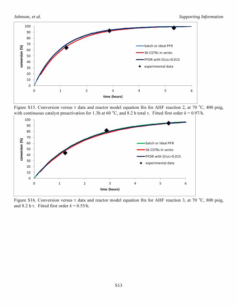
Figure S15. Conversion versus data and reactor model equation fits for AHF reaction 2, at 70
oC, 400 psig,
with continuous catalyst preactivation for 1.3h at 60 oC, and 8.2 h total . Fitted first order k = 0.97/h.
Figure S16. Conversion versus data and reactor model equation fits for AHF reaction 3, at 70
oC, 800 psig,
and 8.2 h . Fitted first order k = 0.55/h.
0
10
20
30
40
50
60
70
80
90
100
0 1 2 3 4 5 6
conv
ersi
on
(%)
time (hours)
batch or ideal PFR
36 CSTRs in series
PFDR with D/uL=0.015
experimental data
0
10
20
30
40
50
60
70
80
90
100
0 1 2 3 4 5 6
conv
ersi
on
(%)
time (hours)
batch or ideal PFR
36 CSTRs in series
PFDR with D/uL=0.015
experimental data
Johnson, et al. Supporting Information
S14
Figure S17. Conversion versus data and reactor model equation fits for AHF reaction 4, at 70
oC, 150 psig,
and 7.5 h total . Fitted first order k = 0.72/h.
Figure S18. Conversion versus data and reactor model equation fits for AHF reaction 5, at 70
oC, 400 psig,
and 8.5 h total . Fitted first order k = 1.29/h.
4. Pressure and gas flow control in second and third generation continuous reactors.
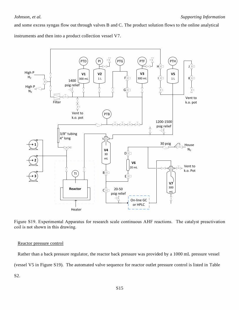
The continuous reactor system used for AHF reactions is shown in Figure S19. Gas reagent is fed from
vessels V1 and V2. The gas flows through valves F and G into vessel V3 and then through four metering
valves. The gas mixes with liquid from the high-pressure pumps and flows into the reactor. Gas and liquid flow
through the reactor co-currently. Gas and liquid continuously flow out of the reactor into vessel V4. Most of
the excess gas flows up into vessel V5, and exits through valves J and K out the vent. Reaction product solution
0
10
20
30
40
50
60
70
80
90
100
0 1 2 3 4 5 6
conv
ersi
on
(%)
time (hours)
batch or ideal PFR
36 CSTRs in series
PFDR with D/uL=0.015
experimental data
0
10
20
30
40
50
60
70
80
90
100
0 1 2 3 4 5 6
conv
ersi
on
(%)
time (hours)
batch or ideal PFR
36 CSTRs in series
PFDR with D/uL=0.015
experimental data
Johnson, et al. Supporting Information
S15
and some excess syngas flow out through valves B and C. The product solution flows to the online analytical
instruments and then into a product collection vessel V7.
Reactor 20-50 psig relief
1200-1500 psig relief
B
C
High P N2
High P H2
V7300
mL
V1300 mL
V21 L
V3300 mL
V51 L
Filter
Vent to k.o. pot
3/8" tubing4" long
J
K H
I
D
E
V620 mL
On-line GCor HPLC
Vent tok.o. pot
Heater
F
G
30 psig House N2
1400 psig relief
PTD PI PTG PTF
PTB
PTH
Vent to k.o. Pot
1
2
3TI
V430
mL
Figure S19. Experimental Apparatus for research scale continuous AHF reactions. The catalyst preactivation
coil is not shown in this drawing.
Reactor pressure control
Rather than a back pressure regulator, the reactor back pressure was provided by a 1000 mL pressure vessel
(vessel V5 in Figure S19). The automated valve sequence for reactor outlet pressure control is listed in Table
S2.
Johnson, et al. Supporting Information
S16
Table S2. Automated valve sequence for control of reactor pressure.
Refer to Figure S19.
Example for keeping reactor outlet pressure between 399.5 psig and 400.5 psig.
It PTH reads > or = 400.5, then valve J opens for 5 seconds, then it closes. This equalizes pressure
between reactor and JK zone.
Valve K opens for 5 seconds, then it closes.
It PTH reads < or = 399.5, then valve H opens for 5 seconds, then it closes.
Valve I opens for 5 seconds, then it closes. This equalizes pressure between reactor and IJ zone.
Repeat.
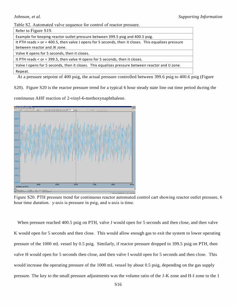
At a pressure setpoint of 400 psig, the actual pressure controlled between 399.6 psig to 400.6 psig (Figure
S20). Figure S20 is the reactor pressure trend for a typical 6 hour steady state line out time period during the
continuous AHF reaction of 2-vinyl-6-methoxynaphthalene.
Figure S20. PTH pressure trend for continuous reactor automated control cart showing reactor outlet pressure, 6
hour time duration. y-axis is pressure in psig, and x-axis is time.
When pressure reached 400.5 psig on PTH, valve J would open for 5 seconds and then close, and then valve
K would open for 5 seconds and then close. This would allow enough gas to exit the system to lower operating
pressure of the 1000 mL vessel by 0.5 psig. Similarly, if reactor pressure dropped to 399.5 psig on PTH, then
valve H would open for 5 seconds then close, and then valve I would open for 5 seconds and then close. This
would increase the operating pressure of the 1000 mL vessel by about 0.5 psig, depending on the gas supply
pressure. The key to the small pressure adjustments was the volume ratio of the J-K zone and H-I zone to the 1
Johnson, et al. Supporting Information
S17
liter vessel V5. The consistent and constant control of reactor pressure enabled the syngas molar gas feed rate
to be controlled more steadily.
Gas feed rate control
The redesign of the molar gas feed rate control used no regulators, no mass flow controller, no mass flow
meters, and no mechanical pumping. Instead, the design concept was to use sequenced automated block valves,
finite volume gas chambers including a large dampening chamber downstream from the automated valves, and
pressure transmitters. Refer to Figure S19. Gas flowed into the reactor through the four metering valves after
V3. The pressure setpoint for 300 mL vessel V3 was automatically adjusted to achieve a desired molar flowrate
of gas through the four metering valves. The automated valve sequence for control of reagent gas molar flow
rate is listed in Table S3. One of the main benefits of controlling gas molar feed rate by this method is that it
works for any gas, or gas mixture, regardless of average gas molecular weight.
Table S3. Automated valve sequence for control of reagent gas molar flow rate.
Refer to Figure S19.
If PTF is less than or equal to “PTF setpoint” (for example 411.4 psig), then valve F opens for 5
seconds, then valve F closes. This equalizes pressure between the gas feed vessel V1 and FG zone.
Valve G opens for 5 seconds, then valve G closes.
Wait “TIME1” seconds.
Calculate mmol/min gas flow rate by using the difference between PTD and PTF , and the current
total sequence time using “TIME1”. Program adjusts “PTF setpoint” to adjust mmol/min gas feed rate toward target.
Repeat.
Each time pressure transmitter PTF would drop below the set point value, automated valves F and G would
cycle through sequence to add more syngas into the 300 mL dampening chamber V3. As such, this would
replenish the gas that flowed into the continuous reactor. The molar gas flow rate was calculated by the known
volume between valve F and valve G, the measured pressure difference between pressure transmitter PTD and
pressure transmitter PTF, and the total time between sequencing. If calculated mass flow rate was higher than
setpoint, then the pressure setpoint for PTF was lowered automatically according to the gain. Likewise, if the
calculated molar gas flow rate was too low, then the pressure setpoint for PTF was automatically increased.
The reagent gas was fed from the 300 mL vessel V1. At higher gas flow rates, both V1 and V2 could be opened
Johnson, et al. Supporting Information
S18
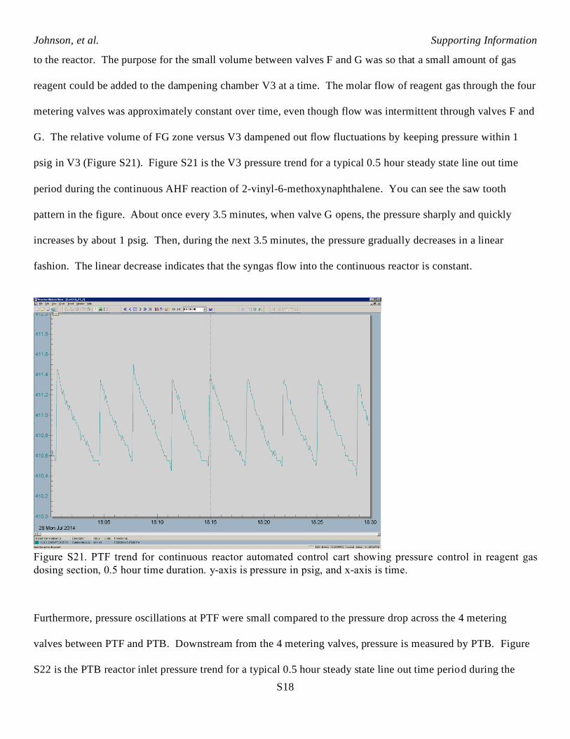
to the reactor. The purpose for the small volume between valves F and G was so that a small amount of gas
reagent could be added to the dampening chamber V3 at a time. The molar flow of reagent gas through the four
metering valves was approximately constant over time, even though flow was intermittent through valves F and
G. The relative volume of FG zone versus V3 dampened out flow fluctuations by keeping pressure within 1
psig in V3 (Figure S21). Figure S21 is the V3 pressure trend for a typical 0.5 hour steady state line out time
period during the continuous AHF reaction of 2-vinyl-6-methoxynaphthalene. You can see the saw tooth
pattern in the figure. About once every 3.5 minutes, when valve G opens, the pressure sharply and quickly
increases by about 1 psig. Then, during the next 3.5 minutes, the pressure gradually decreases in a linear
fashion. The linear decrease indicates that the syngas flow into the continuous reactor is constant.
Figure S21. PTF trend for continuous reactor automated control cart showing pressure control in reagent gas
dosing section, 0.5 hour time duration. y-axis is pressure in psig, and x-axis is time.
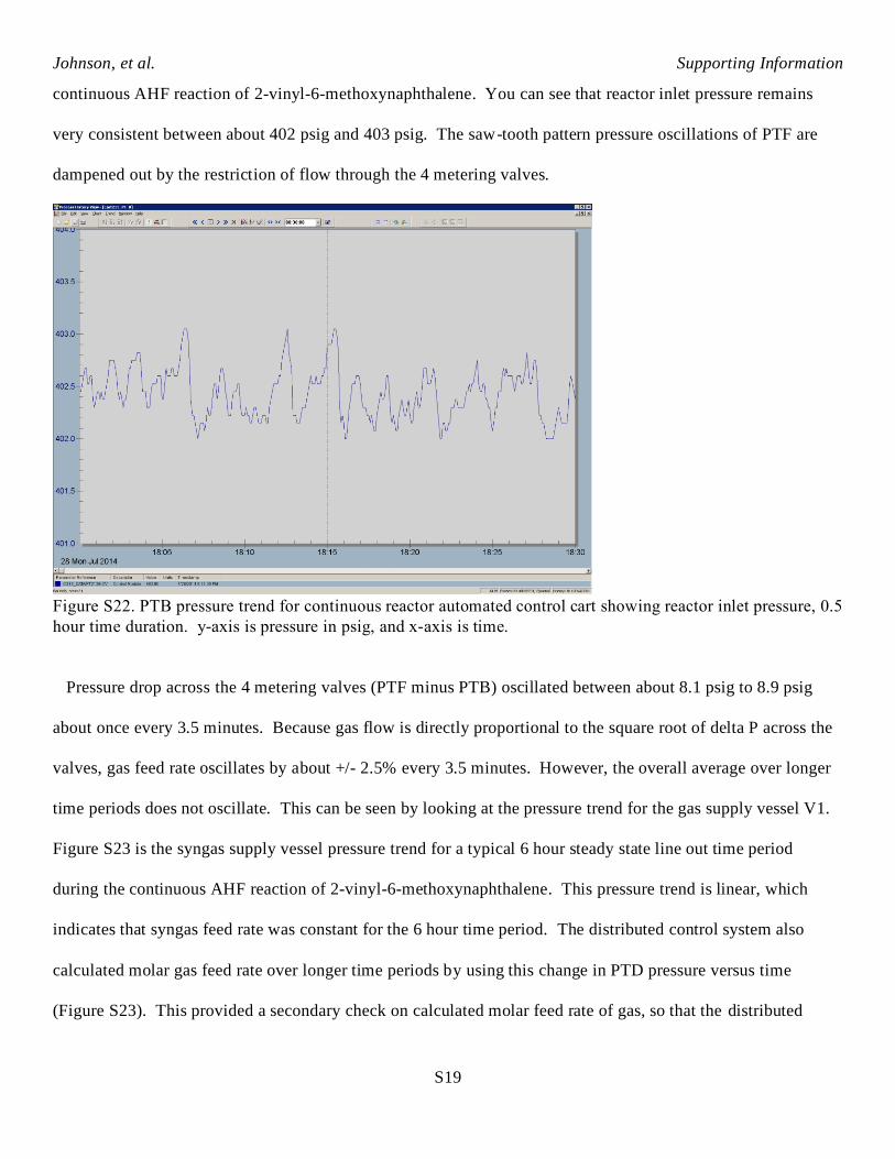
Furthermore, pressure oscillations at PTF were small compared to the pressure drop across the 4 metering
valves between PTF and PTB. Downstream from the 4 metering valves, pressure is measured by PTB. Figure
S22 is the PTB reactor inlet pressure trend for a typical 0.5 hour steady state line out time period during the
Johnson, et al. Supporting Information
S19
continuous AHF reaction of 2-vinyl-6-methoxynaphthalene. You can see that reactor inlet pressure remains
very consistent between about 402 psig and 403 psig. The saw-tooth pattern pressure oscillations of PTF are
dampened out by the restriction of flow through the 4 metering valves.
Figure S22. PTB pressure trend for continuous reactor automated control cart showing reactor inlet pressure, 0.5
hour time duration. y-axis is pressure in psig, and x-axis is time.
Pressure drop across the 4 metering valves (PTF minus PTB) oscillated between about 8.1 psig to 8.9 psig
about once every 3.5 minutes. Because gas flow is directly proportional to the square root of delta P across the
valves, gas feed rate oscillates by about +/- 2.5% every 3.5 minutes. However, the overall average over longer
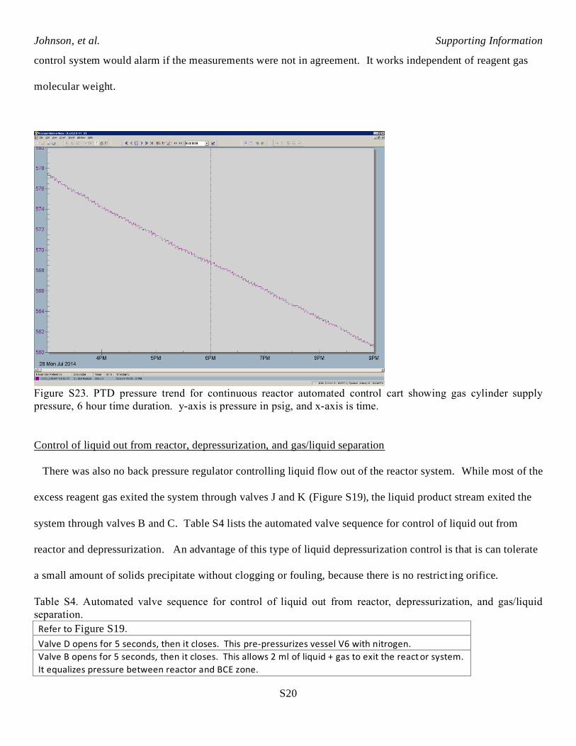
time periods does not oscillate. This can be seen by looking at the pressure trend for the gas supply vessel V1.
Figure S23 is the syngas supply vessel pressure trend for a typical 6 hour steady state line out time period
during the continuous AHF reaction of 2-vinyl-6-methoxynaphthalene. This pressure trend is linear, which
indicates that syngas feed rate was constant for the 6 hour time period. The distributed control system also
calculated molar gas feed rate over longer time periods by using this change in PTD pressure versus time
(Figure S23). This provided a secondary check on calculated molar feed rate of gas, so that the distributed
Johnson, et al. Supporting Information
S20
control system would alarm if the measurements were not in agreement. It works independent of reagent gas
molecular weight.
Figure S23. PTD pressure trend for continuous reactor automated control cart showing gas cylinder supply
pressure, 6 hour time duration. y-axis is pressure in psig, and x-axis is time.
Control of liquid out from reactor, depressurization, and gas/liquid separation
There was also no back pressure regulator controlling liquid flow out of the reactor system. While most of the
excess reagent gas exited the system through valves J and K (Figure S19), the liquid product stream exited the
system through valves B and C. Table S4 lists the automated valve sequence for control of liquid out from
reactor and depressurization. An advantage of this type of liquid depressurization control is that is can tolerate
a small amount of solids precipitate without clogging or fouling, because there is no restrict ing orifice.
Table S4. Automated valve sequence for control of liquid out from reactor, depressurization, and gas/liquid
separation.
Refer to Figure S19.
Valve D opens for 5 seconds, then it closes. This pre-pressurizes vessel V6 with nitrogen.
Valve B opens for 5 seconds, then it closes. This allows 2 ml of liquid + gas to exit the react or system.
It equalizes pressure between reactor and BCE zone.
Johnson, et al. Supporting Information
S21
Valve C opens for 5 seconds, then it remains open. This allows the compressed gas to push liquid out
toward on-line analytical and reaction product collection vessel.
Valve E opens for 20 seconds, then it closes. This pushes liquid toward product collection vessel with nitrogen.
Valve C closes.
Wait time (example 10 minutes)
Repeat.
During normal operation, liquid exiting the reactor continuously collected in the 30 mL vessel V4. About
once every 10 minutes, the liquid was emptied from V4 through valve B. The automated sequence is described
in Table S4. The trapped nitrogen from the 20 mL vessel V6 pushed the liquid sample out through valve C and
over to the online automated sampling and dilution system for online analysis. The liquid flowed from the
online sampling system into a product collection vessel. You can gain an understanding of how this sequence
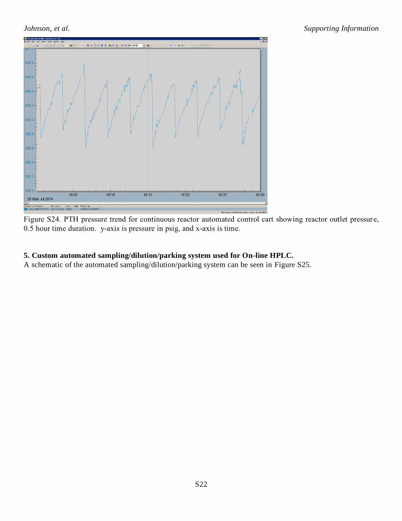
impacted reactor outlet pressure by looking at the pressure trend for PTH. Figure S24 is the reactor outlet
pressure trend for a typical 0.5 hour steady state line out time period during the continuous AHF reaction of 2-
vinyl-6-methoxynaphthalene. You can see the typical sawtooth pressure pattern. Each time valve B opened to
let liquid out of the bottom of V4, reactor outlet pressure suddenly dropped by about 0.9 psig. Thus, reactor
pressure dropped by about 0.2% each time liquid intermittently flowed out of the system, thus pressure deviated
+/- 0.1% from the mean. About every third or fourth sudden pressure decrease was due to valve B opening to
let liquid out of V4. The other downward pressure spikes are due to J opening to let gas out of V5.
Johnson, et al. Supporting Information
S22
Figure S24. PTH pressure trend for continuous reactor automated control cart showing reactor outlet pressure,
0.5 hour time duration. y-axis is pressure in psig, and x-axis is time.
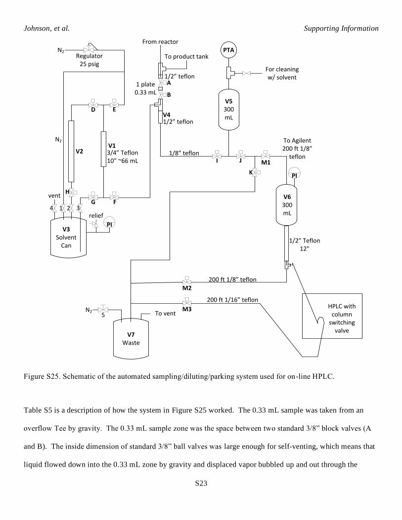
5. Custom automated sampling/dilution/parking system used for On-line HPLC.
A schematic of the automated sampling/dilution/parking system can be seen in Figure S25.
Johnson, et al. Supporting Information
S23
1
A
B
From reactor
1 plate 0.33 mL
D
K
H
E
M1
M2
M3
V5300 mL
V3Solvent
Can
V7Waste
1/2” teflon
To product tank
1/2” teflon
1/2” Teflon12"
G
F
N2
3/4” Teflon10" ~66 mL
I
J
1/8” teflon
HPLC with column
switching valve
200 ft 1/16” teflon
200 ft 1/8” teflon
To Agilent200 ft 1/8”
teflon
To vent
For cleaning w/ solvent
V6300 mL
PI
Regulator 25 psig
2 34
vent
N2
PI
relief
5N2
PTA
V1V2
V4
Figure S25. Schematic of the automated sampling/diluting/parking system used for on-line HPLC.
Table S5 is a description of how the system in Figure S25 worked. The 0.33 mL sample was taken from an
overflow Tee by gravity. The 0.33 mL sample zone was the space between two standard 3/8” block valves (A
and B). The inside dimension of standard 3/8” ball valves was large enough for self-venting, which means that
liquid flowed down into the 0.33 mL zone by gravity and displaced vapor bubbled up and out through the
Johnson, et al. Supporting Information
S24
overflow Tee. The fittings and tubing directly below valve B were 1/2” with no smaller internal restrictions, so
that the 0.33 mL sample would gravity flow down out of the sample zone into vessel V4 when valve B opened.
The vertical dilution solvent measure out zone V1 filled from bottom up, and emptied from top down. This
ensured that it was completely liquid filled, and that it subsequently completely emptied, with only a few
surface drops remaining. It was important to flow in and out of the bottom of the mixing chamber V5. The
nitrogen bubbling action into the bottom of the mixing chamber mixed the diluted sample. The nitrogen
bubbling happened after all of the sample and dilution solvent had been pushed into mixing chamber V5, and
the nitrogen continued to blow through valves E, F, I to pressure up V5. This nitrogen pressure in the mixing
chamber subsequently served to push the diluted sample to V6 near the on-line HPLC through 1.75 mm i.d.
tubing. After mixing, J and M1 valves opened. The vapor/liquid separator vessel V6 served to make sure there
was no gas bubble flowing through the HPLC sample injection loop. Valve M3 opened for a period of time to
flush enough new diluted solution through the HPLC sample injection loop. Then valve M2 opened to push any
excess material to a waste container, and M1 and M2 closed to keep positive pressure on the vapor liquid
separator V6 at all times. Valve K opened to release remaining pressure in the mixing chamber V5 and solvent
measure out zones V1 and V2. The sample was injected on column from the loop by switching valve. The
repeating sequence for the automated valves for the sampling/diluting/parking cart is listed in more detail in
Table S5.
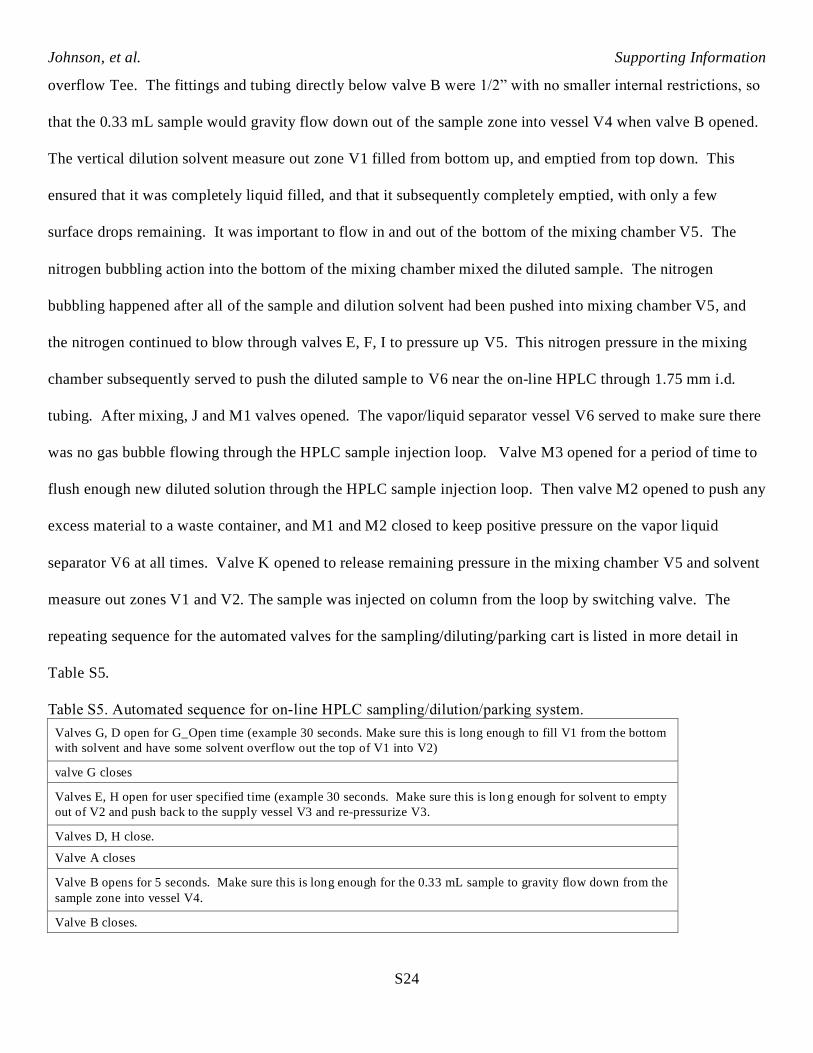
Table S5. Automated sequence for on-line HPLC sampling/dilution/parking system.
Valves G, D open for G_Open time (example 30 seconds. Make sure this is long enough to fill V1 from the bottom
with solvent and have some solvent overflow out the top of V1 into V2)
valve G closes
Valves E, H open for user specified time (example 30 seconds. Make sure this is lon g enough for solvent to empty
out of V2 and push back to the supply vessel V3 and re-pressurize V3.
Valves D, H close.
Valve A closes
Valve B opens for 5 seconds. Make sure this is long enough for the 0.33 mL sample to gravity flow down from the
sample zone into vessel V4.
Valve B closes.
Johnson, et al. Supporting Information
S25
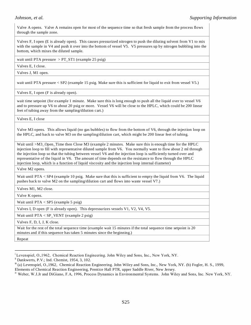
Valve A opens. Valve A remains open for most of the sequence time so that fresh sample from the process flows
through the sample zone.
Valves F, I open (E is already open). This causes pressurized nitrogen to push the diluting solvent from V1 to mix
with the sample in V4 and push it over into the bottom of vessel V5. V5 pressures up by nitrogen bubbling into the
bottom, which mixes the diluted sample.
wait until PTA pressure > PT_ST1 (example 25 psig)
Valves E, I close.
Valves J, M1 open.
wait until PTA pressure < SP2 (example 15 psig. Make sure this is sufficient for liquid to exit from vessel V5.)
Valves E, I open (F is already open).
wait time setpoint (for example 1 minute. Make sure this is long enough to push all the liquid over to vessel V6
and to pressure up V6 to about 20 psig or more. Vessel V6 will be close to the HPLC, which could be 200 linear
feet of tubing away from the sampling/dilution cart.)
Valves E, I close
Valve M3 opens. This allows liquid (no gas bubbles) to flow from the bottom of V6, through the injection loop on
the HPLC, and back to valve M3 on the sampling/dilution cart, which might be 200 linear feet of tubing.
Wait until >M3_Open_Time then Close M3 (example 2 minutes. Make sure this is enough time for the HPLC
injection loop to fill with representative diluted sample from V6. You normally want to flow about 2 ml through
the injection loop so that the tubing between vessel V6 and the injection loop is sufficiently turned over and
representative of the liquid in V6. The amount of time depends on the resistance to flow through the HPLC
injection loop, which is a function of liquid viscosity and the injection loop internal d iameter)
Valve M2 opens.
Wait until PTA < SP4 (example 10 psig. Make sure that this is sufficient to empty the liquid from V6. The liquid
pushes back to valve M2 on the sampling/dilution cart and flows into waste vessel V7.)
Valves M1, M2 close.
Valve K opens.
Wait until PTA < SP5 (example 5 psig)
Valves I, D open (F is already open). This depressurizes vessels V1, V2, V4, V5.
Wait until PTA < SP_VENT (example 2 psig)
Valves F, D, I, J, K close.
Wait for the rest of the total sequence time (example wait 15 minutes if the total sequence time setpoint is 20
minutes and if this sequence has taken 5 minutes since the beginning.)
Repeat
i Levenspiel, O.,1962, Chemical Reaction Engineering. John Wiley and Sons, Inc., New York, NY. ii Dankwerts, P.V.; Ind. Chemist, 1954, 3, 102.
iii (a) Levenspiel, O.,1962, Chemical Reaction Engineering. John Wiley and Sons, Inc., New York, NY. (b) Fogler, H. S., 1999,
Elements of Chemical Reaction Engineering, Prentice Hall PTR, upper Saddle River, New Jersey. iv Weber, W.J.Jr and DiGiano, F.A, 1996, Process Dynamics in Environmental Systems. John Wiley and Sons, Inc. New York, NY.