Modelling the Uncertainty of Slope Estimation from A …gse.vsb.cz/2013/LIX-2013-2-25-39.pdf · MODELLING THE UNCERTAINTY OF SLOPE ESTIMATION FROM A LIDAR-DERIVED ... typically made

25

GeoScience Engineering Volume LIX (2013), No.2

http://gse.vsb.cz p. 25-39, ISSN 1802-5420

MODELLING THE UNCERTAINTY OF SLOPE ESTIMATION FROM A LIDAR-DERIVED DEM: A CASE STUDY FROM A

LARGE-SCALE AREA IN THE CZECH REPUBLIC

MODELOVANIE NEISTOTY VO VÝPOČTE SKLONOV Z LIDAR-OVÝCH DMR; PRÍPADOVÁ ŠTÚDIA VYBRANÉHO MALÉHO

ÚZEMIA V ČR

Ivan MUDRON1, Michal PODHORANYI

2,3, Juraj CIRBUS

1, Branislav DEVEČKA

1, Ladislav BAKAY

4

1 Institute of Geoinformatics, Faculty of Mining and Geology, VSB-TU OSTRAVA, 17.listopadu

15/2172, 70833, Ostrava, Czech Republic

[email protected], [email protected], [email protected]

2 IT4Inovation Centre of Excellence VSB-TU OSTRAVA, 17.listopadu 15/2172, 708 33, Ostrava,

Czech Republic

[email protected]

3 Department of Physical Geography and Geology, Faculty of Science, University of Ostrva,

Chittussiho 10, 710 00, Ostrava, Czech Republic

4 Department of Garden and Landscape Design, Slovak university of Agriculture, Trieda A. Hlinku 2,

949 76, Nitra, Slovak Republic

[email protected]

Abstract

This paper summarizes the methods and results of error modelling and propagation analyses in the Olše

and Stonávka confluence area. In terrain analyses, the outputs of the aforementioned analysis are always a

function of input. Two approaches according to the input data were used to generate field elevation errors which

subsequently entered the error propagation analysis. The main goal solved in this research was to show the

importance of input data in slope estimation and to estimate the elevation error propagation as well as to identify

DEM errors and their consequences. Dependencies were investigated as well to achieve a better prediction of

slope errors. Four different digital elevation model (DEM) resolutions (0.5, 1, 5 and 10 meters) were examined

with the Root Mean Square Error (RMSE) rating up to 0.317 meters (10 m DEM). They all originated from a

LIDAR survey. In the analyses, a stochastic Monte Carlo simulation was performed with 250 iterations. The

article focuses on the error propagation in a large-scale area using high quality input DEM and Monte Carlo

methods. The DEM uncertainty (RMSE) was obtained by sampling and ground research (RTK GPS) and from

subtraction of two DEMs. According to empirical error distribution a semivariogram was used to model spatially

autocorrelated uncertainty in elevation. The second procedure modelled the uncertainty without autocorrelation

using a random N(0,RMSE) error generator. Statistical summaries were drawn to investigate the expected

hypothesis. As expected, the error in slopes increases with the increasing vertical error in the input DEM.

According to similar studies the use of different DEM input data, high quality LIDAR input data decreases the

output uncertainty. Errors modelled without spatial autocorrelation do not result in a greater variance in the

resulting slope error. In this case, although the slope error results (comparing random uncorrelated and empirical

autocorrelated error fields) did not show any statistical significant difference, the input elevation error pattern

was not normally distributed and therefore the random error generator realization is not a suitable interpretation

of the true state of elevation errors. The normal distribution was rejected because of the high kurtosis and

extreme values (outliners). On the other hand, it can show an important insight into the expected elevation and

slope errors. Geology does not influence the slope error in the study area.

26



Abstrakt

Táto práca zhŕňa metódu a výsledky modelovania chýb a analýzu šírenia chýb vo výpočte sklonov

z DMR získaných LIDAR-om v skúmanej lokalite okolia sútoku riek Olše a Stonávka. V terénnych analýzach

výstupy uvedenej analýzy sú vždy funkciou vstupu. Na generovania pola výškových chýb boli použité dve

rozdielne metódy podľa vstupných dát. Modelované chyby v nadmorských výškach následne vstupovali do

analýzy šírenia chýb. Hlavným cieľom práce bolo tak ako aj poukázanie na význam kvality vstupných dát vo

výpočte sklonov a odhad šírenej chyby z nadmorských výšok v sklonoch tak aj identifikácia chýb v DMR a ich

dopad. Závislosti chýb boli vyhodnotené hlavne pre lepší odhad chyby v sklonoch. V simuláciách boli použité 4

vstupné DMR s rozlíšením 0.5, 1, 5 a 10 metrov s RMSE chybou do 0.317 metra (10 m DMR). Všetky DMR

boli získané z mračna bodov získaných LIDAR metódou zberu dát. Šírenie chýb bolo modelované pomocou

stochastickej simulácie Monte Carlo s 250 iteráciami. Článok sa zameriava na šírenie chýb z vysoko presných

vstupných dát na malom území. RMSE chyba bola získaná v prvom prípade z dát získaných terénnym

prieskumom (RTK GPS) a v druhom prípade z porovnania dvoch kvalitatívne rozdielnych DMR. V prvom

prípade sa vypočítali chyby vo výškach pomocou náhodného generátora chýb bez autokorelácie chýb. V druhom

prípade sa s pomocou semivariogramu namodelovalo autokorelované pole chýb vo výškach. Použitím vhodných

štatistík boli odvodené výsledky simulácie a overené stanovené hypotézy. Tak ako sa očakávalo chyby

v sklonoch sú vyššie s zvyšujúcou sa chybou v nadmorských výškach. Tiež závislosti chýb od vypočítaných

sklonov boli preskúmané, kde sa potvrdila závislosť chýb na sklonoch. Na druhej strane geológia nemala žiaden

vplyv na chybu v sklonoch. Chyby namodelované bez autokorelácie nevedú vo väčšine prípadov k štatisticky

významnej odchýlke. Vzhľadom však k rozmiestneniu chýb v priestore (vysoká autokorelácia, zamietnutie

normálneho rozdelenia pre vysokú špicatosť a extrémne hodnoty) nie je táto metóda vhodná. Napriek tomu dáva

dobrú možnosť nahliadnutia do očakávanej chyby v sklonoch a nadmorských výškach.

Key words: Uncertainty, Error propagation, Monte Carlo simulation, LIDAR-derived DEM, Slope

estimation.

1 INTRODUCTION

Although many studies in the field of digital elevation model uncertainty and its error propagation were

carried out, still there are some unacceptable assumptions about the expected error. Firstly, the DEM error

disappears with more precise data acquisition and an optimal interpolation algorithm. Secondly, the DEM error

is thought to be as small as not affecting the outputs of the analyses using a DEM input. Last but not least, DEMs

are assumed and used as error-free models of reality, even though the existence of elevation uncertainty and

gross errors are widely recognized [38], [19]. In the last decades, geomorphometry based on fine topscale DEMs

have become popular in environmental science [35]. The accuracy of a digital elevation model is particularly

important with its intended use [35]. So the misjudgements increased the importance of solving DEMs

uncertainty and the error propagation problem. The awareness that uncertainty propagates through spatial

analyses and may produce poor results that lead to wrong decisions triggered a lot of research on spatial

accuracy assessment and data quality management in GIS (e.g. [33], [10] , [36], [2]) [34]. The information on the

uncertainties in results from Geographic Information Systems (GIS) is needed for effective decision-making.

Current GISs, however, do not provide this information [10], [14], [23]. Furthermore, there is the demand for

presenting a level of accuracy (precision) [23]. Thus the long term vision in the research in spatial data

uncertainty, accordingly DEM as well, was to develop a general purpose “error button” for generating

information systems (GIS) [2]. There are two main ideas how to implement this button. GIS could incorporate

the button into the product metadata [30] or in a more sophisticated solution the button is seen as user-dependent,

which offers various possibilities for refining the error model according to the user’s level of expertise [32]. The

first steps towards the vision became a reality with building a data uncertainty engine, which implements the

general framework for characterising uncertain environmental variables with probability models [34]. According

to the authors, many other research groups worked on the design of an ‘error-aware GIS’, but very few have

reached the operational stage. After the call for the development of geographical information systems that can

handle uncertain data lasting at least for twenty years, Heuvelink, developing the Data Uncertainty Engine

(DUE) engine, filled the gap [34]. Just the first step towards the solution of the error propagation problem was

made. The DUE must be further elaborated and improved. The sustained development of science and technology

brought and will bring new methods of data collection and processing. The DUE as another potential software

application, using different or the same approaches, has to adjust to the changes. The usage of massive high-

resolution DEMs based on the airborne light detection and ranging (LIDAR) renewed some assumptions. Two

important factors appear to explain the lack of scientific knowledge about the use of LIDAR DEMs in an

uncertain-aware terrain analysis. Firstly, it was commonly believed that the high quality of LIDAR DEMs [13],

[1], [20] will make the uncertainty-aware terrain analysis unnecessary. Secondly, uncertainty propagation studies

typically made use of simulation methods, such as simulated annealing and sequential Gaussian simulations [31],

27



that are unsuitable for massive data sets because of their poor scalability [38], [10]. The aim of this paper is to

analyse the aforementioned problems.

2 DEM ERRORS

Spatial uncertainty is defined as the difference between the contents of a spatial database and the

corresponding phenomena in the real world. Because all contents of spatial databases are representations of the

real world, it is inevitable that differences will exist between them and the real phenomena that they purport to

represent [27]. An error is defined as the difference between reality and a representation of reality. In practice,

errors are not exactly known. At best, the distribution of values is known. The chances that the error is positive

or negative are equal [12]. The paper follows the taxonomy in which an error is a measurable and well-defined

(no ambiguities and vagueness in data) part of uncertainty [25]. This is a justifiable choice because the semantics

of elevation do not suffer from conceptual ambiguities which are common in, for example, defining the error in

area-class maps [38]. The detailed process, by which the errors in a DEM are created, depends on the type of

DEM and how it was created. Whatever method is used, DEM estimates are affected by several error sources,

which can be grouped generally under three main classes: accuracy, density and distribution of data, surface

characteristics, and interpolation algorithms [11] [9]. Uncertainty in DEMs originates from two sources, errors in

the lattice (gross, systematic, random) and accuracy loss due to the lattice representation of the terrain [37].

There is a difference between positional and attribute uncertainty. The attribute uncertainty represents the

deviation from true state of height and the positional uncertainty the shift in the object’s position. Understanding

the uncertainty is essential to correct modelling. The most frequent error in standard DEM products is reported

as the Root Mean Squared Error (RMSE). Various methods have been used for estimating the RMSE. Most

recently it is supposed to be estimated by comparison of elevations between well located sites in survey of higher

accuracy with the elevation recorded in DEM at a minimum of 20 test points. The test points may be contour

lines, bench marks, or spot elevations [8]. RMSE is based on the following formula:

n

hzRMSE

2

(1)

where z is the elevation recorded in the DEM; h is the elevation measured with higher precision and n is

the total number of tested locations (at least 20). The Gaussian error model (a mean is the estimate of true values

and a standard deviation is a measure of the uncertainty) makes only the most general assumptions about the

processes by which the error accumulates. [15]. To achieve an improved estimate of the error for any particular

area, a set of measurements made with higher precision is required, at best having another DEM of the same area

with higher precision. In this case, it is possible to compare all values [9]. The spot heights and DEM or both

DEMs have to be constructed separately; the independence is strictly required. When additional information is

available about the structure of errors in the data set, the Gaussian model should be replaced with a substituting

more accurate pattern of error (non-stationary or stationary spatial dependent random error field). According to

previous studies (e.g. [7] [10] [15] [17] [24] [32] [36]), DEM errors are spatially correlated; autocorrelation is a

natural characteristic of the error data. Hunter distinguished three cases of spatial dependences. Case one is

spatial independence (r = 0). The elevation of each point is considered to be spatially independent of its

neighbours (r = 0). In other words, the knowledge of the error present at one point provides no information on

the errors present at neighbouring points, even though the elevation may have similar values. The elevation

realization h at a x, y location is achieved by disturbing each observed elevation z at the same location by an

independent disturbance term N (0, RMSE), which is a normally distributed random variable with a mean 0 and

standard deviation RMSE (Eq. 2):

),0(),(),( RMSENzh yxyx (2)

Case two is spatial dependence (limit r =1). At the other extreme, spatial autocorrelation reaches its

maximum. All errors are perfectly correlated, and there is only 1 degree of freedom in effect in the disturbance

field being applied to the DEM. It is unlikely that any DEM production process would generate a systematic

error in elevations. Case three is spatial dependence (0 < R < 1). The case of positive correlation less than 1 is

clearly most realistic [15] and the disturbance N(0,RMSE) is spatially correlated to a certain range following the

fitted error model. Exponential and Gaussian [38] spatial autocorrelation models were selected to represent the

correlation of the DEM error in the DEM uncertainty propagation studies. First exponential and later Gaussian

models were found to be realistic and suitable for topography [31]. The study investigates the type of the model,

range and the spatially independent random error pattern [10].

28



2.1 Error propagation analysis

There are two main approaches to the error propagation of a continuous variable: the analytical and the

numerical error propagation. The analytical error propagation method uses an explicit mathematical model to

describe the mechanisms of error propagation for a particular multi-criteria decision rule [6]. In numerical

methods, the calculations are not made with exact numbers. Numerically generated random data sets are used

instead of exact numbers. Usually they are generated on a computer in case of too complicated data or a physical

model for analytical approach. In this study, the simulation of error was made stochastically using a Monte Carlo

simulation. This method is further subdivided into unconditioned and conditioned models [5]. Unconditional

error simulation models are based on the number of realizations of random functions. At their most basic level,

they comprise an algorithm to select independent and uncorrelated values drawn from a normal distribution

which can be added to the original DEM. The problem with unconditioned simulations is that they still make the

assumption that the pattern of error is uniform over the study area or a wider region. Conditional error models

directly honour observations of error at the sample locations. Such observations might have been obtained by

comparison between the DEM and a higher accuracy reference data set collected from the same area [5]. In else,

the parameters of an error model vary depending on the specific location. Comparing the results of using

different methods of error modelling, the best method, which gives widely implementable and defensible results,

is that based on a conditional stochastic simulation [9]. The most common uncertainty propagation analysis

approach makes use of a Monte Carlo stochastic simulation [22]. The utilisation of a Monte Carlo simulation,

which is the most flexible method for investigating the propagation of uncertainty in terrain analysis, is time-

consuming [17]. Despite this drawback the unconditional Monte Carlo simulation was used to propagate the

error. Tab. 1 shows the computation time cost for one simulation [10] modelled by the software R.

Tab. 1 Computational time for modelling one error pattern

DEM resolution Number of points Elapsed Time

10 x 10 263 520 2 min 21 sec

5 x 5 1 051 997 40 min 57 sec

1 x 1 26 289 516 17 days 2 hrs

1 x 1 1275630 1 hr 1 min 38 sec

0.5 x 0.5 5051130 16 hrs 54 min 33 sec

Although the area is relatively small (11.26 km2 respectively 1.25 km

2) and the relative difference in

elevation less than 45 meters, the empirical error pattern was investigated to find out an anomaly or a trend

within. None of it was found in the error pattern. The outline of the Monte Carlo simulation is shown in Fig. 1

(used SW ArcGIS, own programming in C++ to calculate statistics). In simulations the initial DEM was used

(with a resolution of 0.5, 1, 5, 10 m). This DEM was considered as an error free representation of the true state of

elevation. Next the “error free slope” slope estimate was calculated. Then DEM error patterns were generated

according to the initial DEM and error model attributes. The initial DEM was perturbed with the generated

random error field (with and without autocorrelation). The resulting DEM had the essential properties of both the

error pattern and the initial raster. Thus 500 realizations of DEM (250 both with and without autocorrelation)

were generated and subsequently slope estimates were derived from alternative DEMs. The set of error patterns

in slopes was calculated as the difference between the error free slope and the particular alternative slope. Using

appropriate statistics the results of the simulation were derived. In some cases the absolute error value had to be

used instead of the error value [10].

29



Fig.1 Outline of Monte Carlo simulation, here 1) denotes input DEM, 2) SLOPE calculated from 1 3) generated

DEM ERROR, 4) Alternative DEM, 5) Alternative slope, 6) Error in slope, 7) Statistics.

2.2 Algorithm of slope computation

A variety of methods can be used to estimate the slope from DEM. Weighted least squares fit of a plane

to a 3x3 neighbourhood centred on each point is the most amenable to a mathematical analysis of error

propagation [15]. Most of the GIS SWs (including the most used ArcGIS) use this method to compute the slope

from a DEM. In this paper, we decided to follow the aforementioned method’s algorithm. The output slope

derivate can be calculated in degrees (angular unit Eq. 8) or percentage (Eq. 7). The chosen units were degrees.

The slope in degrees is calculated multiplying the slope in radians with 57.29578. The slope calculation (Fig. 2)

is based on the change of height (rise) in the direction of x and y direction (run) - mathematically the first partial

derivation of z in x and y axes. Thus the slope (Eq. 5) is determined by the rate of change (Beta) in both

horizontal (HD Eq. 3) and vertical (VD Eq. 4) directions from the centre cell (E).

x

zHD

(3)

y

zVD

(4)

The approximation of the partial derivatives was made by a third-order finite difference method (Eq. 5

and 6) [18]. The method uses the 3x3 neighbourhood (Fig. 3) of the elevation values obtained in the raster

around the centre cell. The distance between the elevation points denoted as wand represents also the cell (pixel)

size of raster [10].

Fig. 2 Left the 3x3 neighbourhood window of the centre cell E and right the rise, run and beta description.

30



w

GDAIFCHD

*8

22 (5)

w

IHGCBAVD

*8

22 (6)

22 VDHDS (7)

22arctan VDHD (8)

The influence of data precision on the derived slope is highly related to grid resolution. While using a

high-resolution DEM (e.g. 1 m grid resolution), the influence of data precision becomes quite significant. DEM

resolution determines the level of details of the surface being described. It naturally influences the accuracy of

derived surface parameters. On the other side, usually the DEM error caused by data precision level is quite

minimal, except in flat areas where the rounding errors could be significant [Zhou, Liu, 2004]. The precision

significance was investigated as well, to prove or reject. We tried to minimize the rounding error because of flat

areas [10].

3 STUDY AREA

The error propagation was carried out along a 5.9 km stretch of the Olše River and a 3.2 km stretch of the

Stonávka River. Both river sections are located in the northeast region of the Czech Republic near its border with

Poland [16].The area is located south of the town of Karviná in the north-eastern part of the Moravian-Silesian

Region. The area is 5.544 km in length and 2.281 km in width spaced. After the area affected with gross error

was eliminated, a total area of 11.262 km2

remained. Because of gross errors and uncertainty in the data

collection process caused by the atmosphere, three parts of the area (west) had to be clipped. Due the time-

consuming computational method the 1.250 km2 large study was used in case of a higher precision data input

(Fig. 3). The elevation of the area varied between 211 and 256 (respectively 216 to 227 for small area) meters

over the sea level. The slope varied from 0°to 85° (respectively 0 to 67 degrees). The average slope values (1.95°

to 3.9° respectively 3° to 3.5°) and the data histograms revealed flat characteristics of the surface with few steep

slopes [10].

Fig. 3 Study area and measurement point locations for RMSE computation

31



4 DATABASE CREATION

The GIS database comes from various sources, each having its own level of uncertainty, depending on the

specific technique used to acquire it [14]. The input data used to create the DEM in this study were obtained

using the LIDAR method (Light Detection and Ranging). The Swedish company TopEyeAB, working with the

MK-II laser system of its own design, carried out flights over the research area. The system consisted of a laser

scanner with a 50 kHz frequency, the Inertial Navigation System (INS) and the Global Positioning System (GPS)

systems. The optical portion of the scanner deviated the laser beam into circular traces. The system was equipped

with the Rollei digital air camera with a 16-megapixel resolution (4080 x 4076 pixels). The scanning was carried

out on the D-Hahn helicopter carrying the MKII-S/N 804 system at an altitude of 250 m [16]. The DEMs (0.5, 1,

5 and 10 m resolution) were computed independently of each other from a particular acquired LIDAR data point

cloud. The density of all data points was 19 points per square meter. The density of terrain points was 9 points

per square meter. The points were classified into three categories: terrain, vegetation under and over 3.5 meters

high. The RMSE in input data were calculated two times for every DEM to make the comparison of possible

inputs. First the error values were calculated subtracting the DEM from the DEM with higher precision

(resolution). The 0.2m resolution DEM was used for the 0.5m resolution DEM. Then the RMSE (0.317 for 10 m,

0.156 for 5 m, 0.04 for 1 m and 0.035 for 0.5 meter resolution) was calculated from the error values of the whole

area. This RMSE values were compared with the result of the second computation which was computed from 49

point measurements in the study area (Fig. 3). 22 of 49 points were created by CUZK (Land Survey Office of

Czech Republic) without any given information of the data gathering method and accuracy. The second RMSE

computation had a higher RMSE, which was effected by the location (sinking ground of mining area) of the 49

points. These are also not representative for the whole area and location. The 49 points were located often in

error prone surfaces (roadsides, river bank sides). The 10m resolution RMSE difference takes 5.7 cm (0.374 for

49 points and 0.317 for LIDAR), which is 17 % of the total value of the LIDAR RMSE. In other cases, it was

even worse (5 m – 14.1 cm, 1 and 0.5 m – 24.9 cm). It is necessary to mention that the LIDAR DEM of higher

accuracy showed a certain uncertainty too. LIDAR RMSE results were taken to fit the spatially uncorrelated

error pattern as a consequence of a better representation of the continuous empirical error pattern. The

autocorrelated error pattern was made by investigating the empirical elevation error (Chapter 5.1).

4.1 Simulation of random fields

The input error field was made by the investigation of the empirical error pattern obtained with the

aforementioned method (Chapter 2). The error propagation was modelled both with and without a spatially

autocorrelated error field. The real state of nature was other than the expected theoretical state. First, there is an

unjustified assumption that the mean error is zero [37]. The error mean statistics were close to zero, but all of

them were rejected as statistical zeroes using a t-test hypothesis test in the Statgraphics software (Tab. 2).

Tab. 2 DEM error statistics (Number of Elevation Points (samplings), Error Mean [meters], Standard Deviation

of Error [meters], and Maximum Absolute Error [meters])

DEM resolution NUMBER OF POINTS MEAN STD.

DEVIATION

MAX ABS ERROR

10 x 10 263 520 -3.2 10-2 0.692 11.942

5 x 5 1 051 997 -1.2 10-3 0.362 12.053

1 x 1 26 289 516 -2.3 10-3 0.085 9.567

0.5 x 0.5 83 963 724 1.0 10-5 0.008 1.597

The best fit of the elevation error pattern is to follow the empirical model [9]. If the difference between

the elevation in the DEM and the actual surface (which equals the error surface) is done, the error surface should

have a large positive autocorrelation [26] [28] [29] [30]. It is assumed that the RMSE over the study area is

constant or spatially autocorrelated, which was confuted in previous researches (Fisher, Oksanen etc.). Although

the total area is 11.262 km2 small and according to the terrain surface and the aforementioned research results

(RMSE should be constant), it was necessary to divide it into smaller subareas, where this statement was proved.

Any significant difference in parameters (range, partial sill and nugget) was not found. The area was searched for

trends. But none of them was found. The best fitted model was the Stable one. According to previous researches

the Exponential and Gaussian models were chosen to fit the pattern as well. The Gaussian and Spherical models

had almost the same results, but the Gaussian one better fitted the closest averaged values and that is why it was

chosen (Tab. 3, Fig. 4, Fig. 5). The appropriate shape of the model was not so critical as the computed

autocorrelation parameters.

32



Tab. 3 Gaussian error model parameters

DEM

resolution

Lag Size [m] Num. of Lags Nugget [m] Partial Sill [m] Range [m]

10 x 10 10 12 0.254 0.163 52.925

5 x 5 5 12 0.068 0.042 31.100

1 x 1 1 12 8.7 10-4 3.3 10-3 8.178

0.5 x 0.5 0.5 12 3.2 10-5 2.7 10-5 3.897

Fig. 4 Gaussian error model for 1x1m resolution DEM

Fig. 5 Gaussian error model for 0.5x0.5m resolution DEM

The theoretical Gaussian models were used to model the fields; Fig. 8 depicts the difference between the

spatially correlated and uncorrelated random fields (10 m DEM). The error fields were modelled 250 times for

each DEM to perform the Monte Carlo simulation. The outputs of the aforementioned stochastic error

propagation (Fig. 1) are mentioned in the following chapter results. The theoretical Gaussian error model of

0.5m resolution (Fig. 5) opens a question about the threshold; whether it is reasonable to use a spatially

autocorrelated model or just white noise [10].

33



Fig. 6 Left uncorrelated white noise (10x10_rndom1) and right spatially correlated random error field (10x10_1)

of 10 m DEM; randomness represented by granulation (left) and clustering of shades of grey (right) are

obviously different instances and also inputs of error propagation analyses.

5 RESULTS

The error propagation results are summarized in Tab. 4. For example, in case of 10x10 m DEM the error

input is expected to be 1.11° (respectively 0.66° without spatial autocorrelation) large slope error (the mean of

the means in column 5). For 5x5 m it is 1.08° (0.64°), 1x1 m 1.24° (0.78°) and for 0.5x0.5 m 2.18° (1.39°). The

greatest difference was in case of the 0.5x0.5m DEM resolution. The results are represented in absolute values.

The behaviour of the error when the value x and its opposite value –x represent the same deviation from the real

state of nature, made this representation possible. It is more natural to see the errors in positive values and it

enables better interpretations. The most representative number in the evaluation of errors, then it is the mean.

Fifty spot samples were randomly selected to prove the insignificant difference between the slope error result

derived from the inputs with and without autocorrelation [10] (Statgraphics SW).

Every spot sample has 250 alternative values which were used to compute a mean and standard deviation. Two

sample F test (standard deviation) and two sample t rest (mean) were used. The null hypothesis was set to: There

is no difference in the standard deviations (respectively a means) and the alternative hypothesis to: There is

statistically significant difference between the standard deviations (means). For example for the 1x1m resolution

we discovered that 46 in 50 cases for the mean, respectively 43 in 50 for the standard deviation do not differ

significantly. The errors without spatial autocorrelation do not result in a greater variance in the resulting slope

error (Oksanen got the same results). Although some statistically significant deviations (small values of slope

error means related to steeper surfaces and almost half of the values in case of 0.5x0.5m resolution) were found,

it is possible to state that majority of the results computed from the elevation field without autocorrelation is

slightly underestimated. Thus, it is possible that the use of less appropriate input data can lead to approximate the

estimation of slope error, which is slightly underestimated [10].

The outliners have to be also incorporated in the error model which was not done due to the lack of time. The

outliers were investigated only in the case of 10x10m resolution DEM (Fig. 9). They were connected with

specific land cover types – steep slopes of roadsides, dump sides and river banks. The RMSE of the modelled

elevation error pattern increased to 0.300 m by incorporating the outliners, which is close to the RMSE of the

empirical elevation error pattern (0.317). The average mean decreased from -3.2 10-2

to -2.9 10-3

. The outliers

were almost uniformly distributed with a mean value of -2.15 for the negative (respectively 2.06 for positive)

outliers. Incorporating the outliers increased the average error slope from 1.11° to 1.24° [10].

The influence of elevation error was investigated comparing the LIDAR DEM with the photogrammetric DEM

of the same 10x10m resolution and area. As expected the error in slopes increases with the vertical error in

elevation. Using the LIDAR input for the 10m DEM the average slope error decreased to 78.36 % of the

photogrammetric input [10].

34



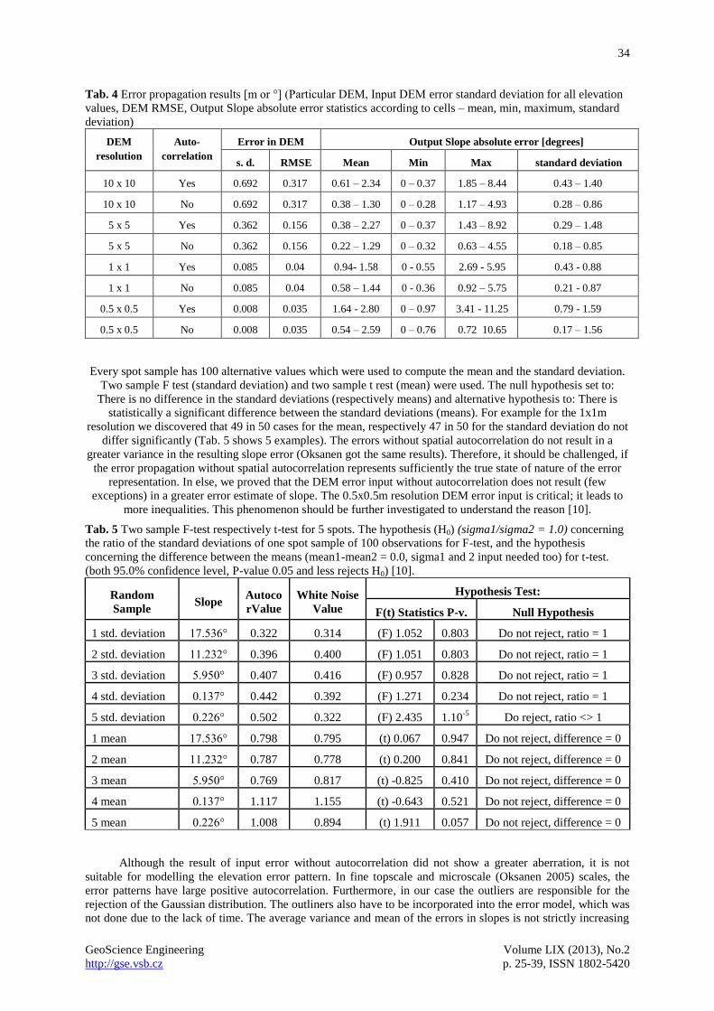
Tab. 4 Error propagation results [m or °] (Particular DEM, Input DEM error standard deviation for all elevation

values, DEM RMSE, Output Slope absolute error statistics according to cells – mean, min, maximum, standard

deviation)

DEM

resolution

Auto-

correlation

Error in DEM Output Slope absolute error [degrees]

s. d. RMSE Mean Min Max standard deviation

10 x 10 Yes 0.692 0.317 0.61 – 2.34 0 – 0.37 1.85 – 8.44 0.43 – 1.40

10 x 10 No 0.692 0.317 0.38 – 1.30 0 – 0.28 1.17 – 4.93 0.28 – 0.86

5 x 5 Yes 0.362 0.156 0.38 – 2.27 0 – 0.37 1.43 – 8.92 0.29 – 1.48

5 x 5 No 0.362 0.156 0.22 – 1.29 0 – 0.32 0.63 – 4.55 0.18 – 0.85

1 x 1 Yes 0.085 0.04 0.94- 1.58 0 - 0.55 2.69 - 5.95 0.43 - 0.88

1 x 1 No 0.085 0.04 0.58 – 1.44 0 - 0.36 0.92 – 5.75 0.21 - 0.87

0.5 x 0.5 Yes 0.008 0.035 1.64 - 2.80 0 – 0.97 3.41 - 11.25 0.79 - 1.59

0.5 x 0.5 No 0.008 0.035 0.54 – 2.59 0 – 0.76 0.72 10.65 0.17 – 1.56

Every spot sample has 100 alternative values which were used to compute the mean and the standard deviation.

Two sample F test (standard deviation) and two sample t rest (mean) were used. The null hypothesis set to:

There is no difference in the standard deviations (respectively means) and alternative hypothesis to: There is

statistically a significant difference between the standard deviations (means). For example for the 1x1m

resolution we discovered that 49 in 50 cases for the mean, respectively 47 in 50 for the standard deviation do not

differ significantly (Tab. 5 shows 5 examples). The errors without spatial autocorrelation do not result in a

greater variance in the resulting slope error (Oksanen got the same results). Therefore, it should be challenged, if

the error propagation without spatial autocorrelation represents sufficiently the true state of nature of the error

representation. In else, we proved that the DEM error input without autocorrelation does not result (few

exceptions) in a greater error estimate of slope. The 0.5x0.5m resolution DEM error input is critical; it leads to

more inequalities. This phenomenon should be further investigated to understand the reason [10].

Tab. 5 Two sample F-test respectively t-test for 5 spots. The hypothesis (H0) (sigma1/sigma2 = 1.0) concerning

the ratio of the standard deviations of one spot sample of 100 observations for F-test, and the hypothesis

concerning the difference between the means (mean1-mean2 = 0.0, sigma1 and 2 input needed too) for t-test.

(both 95.0% confidence level, P-value 0.05 and less rejects H0) [10].

Random

Sample Slope

Autoco

rValue

White Noise

Value

Hypothesis Test:

F(t) Statistics P-v. Null Hypothesis

1 std. deviation 17.536° 0.322 0.314 (F) 1.052 0.803 Do not reject, ratio = 1




5 std. deviation 0.226° 0.502 0.322 (F) 2.435 1.10-5

Do reject, ratio <> 1

1 mean 17.536° 0.798 0.795 (t) 0.067 0.947 Do not reject, difference = 0


3 mean 5.950° 0.769 0.817 (t) -0.825 0.410 Do not reject, difference = 0

4 mean 0.137° 1.117 1.155 (t) -0.643 0.521 Do not reject, difference = 0


Although the result of input error without autocorrelation did not show a greater aberration, it is not

suitable for modelling the elevation error pattern. In fine topscale and microscale (Oksanen 2005) scales, the

error patterns have large positive autocorrelation. Furthermore, in our case the outliers are responsible for the

rejection of the Gaussian distribution. The outliners also have to be incorporated into the error model, which was

not done due to the lack of time. The average variance and mean of the errors in slopes is not strictly increasing

35



with steepness of the slope (e.g. Fig. 7). This causality should be further investigated; one of the reasons is the

insufficient number of samples with a steeper slope. The prevailing spatial distribution of slopes in study is also

partially captured in the mean slope error (Fig. 7, Fig. 8). The input based on the empirical elevation error (AC)

describes better the error pattern and leads to a more realistic and accurate spatial distribution of slope errors

according to the slope in the study area. The white noise (WN) input error field is closest to AC in a minimum

slope error distribution. Linear planar surfaces (roads etc.) are inadequately propagated. Planar surface is the

most error prone type. According to similar studies (Fisher, Goodchild etc.) using different DEM input data, the

high quality LIDAR input data decreases the output uncertainty. In our case, the autocorrelated model fitted the

error surface with exception of its outliers. Extreme values are higher in case of the theoretical model with

autocorrelation; a random number generator produces smaller extreme values as well. Autocorrelation also

expands the standard deviation of extreme values. On the one side, the extreme elevation error values were found

to be clustered around the steepest slopes, on the other side, the steeper slopes has a smaller slope error result

with the same elevation error input. The range of the fitted empirical error model (49.6 for 10x10, 31.1 for 5x5,

13.8 for 1x1 and 3.9 for 0.5x0.5) was decreasing with a higher resolution. We do assume that there should be a

specific resolution limit value where the range is close to 0. Geostatistical modelling is very time consuming. We

had to decrease the extent for the 0.5x0.5 and 1x1 meter resolution inputs. To compute one 1x1meter DEM

resolution error pattern (21 983 304 values in 5964 rows and 3686 columns) took 12 days and 17 hours (using 30

GB RAM and 4 processors Intel(R) Core (TM2)2 Quad CPU Q9300, 2.5 GHz). This computation requires a

super-computer.

Fig. 7: Slope error dependent variable (vertical axis) vs. Slope independent variable (horizontal axis) (WN

randomly generated white noise, AC autocorrelation input according to empirical error pattern) showing the

decrease in slope error with increasing slope

Fig. 8 Left the slope estimate (5x5 LIDAR DEM) and right the stochastic Monte Carlo result of an average slope

error for cells in a 5x5m resolution. The flat plain areas are the most error prone surfaces and have black colour

in the slope error image

36



Fig. 9 The statistics important to reconstruct the slope error distribution - mean, a variance (var), minimum (min)

and maximum (max) for 10x10m slope errors calculated from the autocorrelated input (AC) and the white noise

input (WN); the darker the colour, the higher the slope error value and the more planar the surface (see fig. 6).

The distribution of errors is normally distributed with the mean and variance (resp. standard deviation) value,

outliers represent the maximum and minimum value. These inputs are necessary to the best description of the

possible error in the result.

5 DISCUSSION

Although a lot of research has been made in the uncertainty and error propagation field over the last

decades, still many questions left unanswered. In this study, we focused on clearing antagonistic results provided

by Oksanen and Fisher. Oksanen declared that slope errors modelled without autocorrelation do not show worse

results. In else, the slope derivate has not a maximum variation with a spatially uncorellated random error. On

the other side, Fisher declared that the slope derivate computed from the uncorrelated random error is a worse

result because of a poor input elevation error representation. We found out that Oksanen is right. Fisher is correct

about the poor representation and that the research area should be always investigated before analysed. We were

not able to completely ascertain the character of the pattern error. Definitely, the underlying error pattern was

found. Some irregular outliners appeared which have to be incorporated. The next step should be the

investigation of the outliners. The empirical error model and the modelled error model have to be subtracted and

the product investigated (external data may help too – underlying geology, terrain roughness, land use, etc.). The

resulting pattern is an addendum to the underlying error pattern. There can be more functions describing local

shapes of error pattern. Sum of all functions (patterns) gives the resulting error pattern. We found that there

should be a threshold value, which in case of high precision and resolution data do not require the usage of

autocorrelation in error surface (in case of the high precision LIDAR data input and a relatively small area).

It is true that any given input data carry an error value significant enough to change the resulting slope – even the

high precision micro-scale LIDAR DEM. The results obtained with DEM inputs of the same resolution and

acquired with other methods (photogrammetric) could be used for a better comparison and calculation of the

exact LIDAR improvement in slope error estimation. Other software tools should be used to prove the simulated

reality with gstat. Because of the time demanding computational process, less consuming processes should be

investigated for the error pattern simulation, e.g. a fuzzy approach. The software development and new

37



supercomputers could be another solution. There is still a doubt, pros and cons, whether the unconditional

Gaussian or sequential Gaussian simulation has to be used, how to model a non-stationary error field in larger

areas and what it is dependent on?

It is necessary to remember the main reason for dealing with the uncertainty: decreasing the risk that the

outcome will be incorrect and will lead to wrong decisions. This study was made as an error propagation

background to inundation area delineation with a GLUE method in the area. The processing of airborne

hyperspectral data introduces an uncertainty which is sufficient to change the product. To know the uncertainty

in the result is important in crisis management and other fields. Sometimes even one degree in slope can change

the situation and flooded area.

6 CONCLUSIONS

The main goals were fulfilled. Thus, the error assessment is an inevitable part of every result presentation.

The deviations or the uncertainty of outputs, which we have to be taken into account, should be presented.

Although there are high quality input data, they also introduce a certain uncertainty which can lead to a change

in decisions and have further consequences. So the use of high quality data does not make the uncertainty

analyses unnecessary.

Regarding to similar studies using different DEM input data, the high quality LIDAR input data decrease the

output uncertainty. The comparison with photogrammetric data input in our study area proved and emphasised

the statement that increased precision in input data decreases the uncertainty in result.

Although the result of input error without autocorrelation did not show a greater aberration, it does not interpret

and reflect the properties of real error pattern. In fine topscale and microscale scales, the error pattern has large

positive autocorrelation and its distribution is not the Gaussian one. In our case, the outliers (extreme values) are

responsible for the rejection of the Gaussian distribution. These outliers were investigated and reasoned. The

normal distribution was rejected because of the high kurtosis as well. Therefore, the realization of a random error

generator is not suitable interpretation of the true state of elevation errors. On the other side, it can show an

important insight into expected elevation and slope error. It is possible to improve the error result using

dependencies (in our case between slope error and slope, elevation error outliers and specific land use types) and

the fact that the error result (for random white noise input) is slightly underestimated. Geology does not

influence the slope error in the study area.

The underlying error pattern has to incorporate the outliers too. If there are any of them, then the sources of them

must be found. The simulated error pattern has to be as closest as possible to the empirical one. Error

propagation is irrelevant without a proper reconstruction of the empirical input error pattern. The research area

should be always investigated before analysed.

Acknowledgement

This paper was elaborated in the framework of the IT4Innovations Centre of Excellence project, reg. no.

CZ.1.05/1.1.00/02.0070 supported by the Operational Programme 'Research and Development for Innovations’

funded by the Structural Funds of the European Union and the state budget of the Czech Republic and the

research project SGS - SPP SV51122M1/2101 (Vliv extrémních přírodních jevů a rizik na ekonomickou činnost

člověka v krajině).

REFERENCES

[1] C.P. Barber, A. Shortage, Lidar elevation data for surface hydrologic modeling: Resolution and

representation issues, Cartography and Geographic Information Science, 2005, vol. 32 (4), pp. 401-410.

[2] S. Openshaw, M. Charlton, S. Carver, Error propagation: A Monte Carlo simulation in Masser, Longman

Scientific and Technical, London, 1991.

[3] W. Shi, P.F. Fisher, M.F. Goodchild, Spatial Data Quality, Taylor & Francis, London, 2002.

[4] S. Erdogan, Modelling the spatial distribution of DEM error with geographically weighted regression: An

experimental study, Computers & Geoscience, 2010, vol. 36, pp. 34 – 43.

[5] P.F. Fisher, N.J. Tate, Causes and consequences of error in digital elevation models, Progress in Physical

Geography, 2006, vol. 30 (4), pp. 467-489.

[6] J.R. Eastman, P.A.K. Kyem, J. Toledano, W. Jin, GIS and decision making, Explorations in Geographical

Information Systems Technology, 1993, vol. 4.

[7] P.F. Fisher, First experiments in viewshed uncertainty: the accuracy of the viewable area,

Photogrammetric Engineering and Remote Sensing, 1991, vol. 57, pp. 1321-1327.

[8] P.F. Fisher, First experiments in viewshed uncertainty: simulating fuzzy viewsheds, Photogrammetric

Engineering and Remote Sensing, 1992, vol. 58 (3), pp. 345-352.

38



[9] P.F. Fisher, Improved modeling of elevation error with geostatistics, Geoinformatica, 1998, vol. 2 (3), pp.

215-233.

[10] Mudron, I., Podhoranyi M., Cirbus J.: Modelling the Uncertainty of Slope Estimation from LIDAR -

derived DEM: A Case Study from Large-Scaled Area in Czech Republic in Sympozia GIS Ostrava 2012

Proceedings - Surface Models for Geoscience, Ostrava 23. - 25.1.2012, ISBN 978-80-248-2558-8

[11] J. Gong, L. Zhilin, Q. Zhu, H.G. Sui, Y. Zhou, Effect of various factors on the accuracy of DEMs: an

intensive experimental investigation, Photogrammetric Engineering and Remote Sensing, 2000, vol. 66

(9), pp. 1113–1117.

[12] G. B. M. Heuvelink, Error-Aware GIS at work: real-world applications of the data uncertainty engine,

Remote Sensing and Spatial Information Sciences, 2007, vol. 34.

[13] M.E. Hodgson, J. Jensen, G. Raber, J. Tullis, B.A. Davis, G. Thompson, K. Schuckman, An evaluation of

lidar-derived elevation and terrain slope in leaf-off conditions, Photogrammetric Engineering and Remote

Sensing, 2005, vol. 71 (7), pp. 817-823.

[14] D. Hwang, H.A. Karimi, D.W. Byun, Uncertainty analysis of environmental models within GIS

environments, Computers & Geosciences, 1998, vol. 24 (2), pp. 119-130.

[15] G.J. Hunter, M.F. Goodchild, Modelling the uncertainty of slope and aspect estimates derived from

spatial database, Geographical Analyses, 1997, vol. 29 (1), pp. 35-49.

[16] M. Podhoranyi, J. Unucka, P. Bobal, V. Rihova, Effects of Lidar DEM resolution in hydrodynamic

modelling: model sensitivity for cross-sections, International Journal of Digital Earth 2012.

[17] J. Oksanen, T. Sarjakoski: Non-stationary modelling and simulation of LIDAR DEM uncertainty in

Accuracy, in: 2010 Symposium, Leicester, UK, 2010

[18] A. K. Skidmore, A comparison of techniques for calculating gradient and aspect from a gridded digital

elevation model, International Journal of Geographical Information Systems, 1989, vol. 3, pp. 309 – 318.

[19] K. Trolegårt, A. Östman, R. Lindgren, A comparative test of photogrammetrically sampled digital

elevation models, Photogrammetria, 1986, vol. 41, pp. 1–16.

[20] J. Vaze, J. Teng, High resolution LIDAR DEM – How good is it?, Modelling and Simulation, 2007, pp.

692-698.

[21] Q. Zhou, X. Liu, Analysis of errors of derived slope and aspect related to DEM data properties,

Computers & Geosciences, 2004, vol. 30, pp. 369–378.

[22] J. Beekhuizen, G.B.M. Heuvelink, I. Reusen, J. Biesemans, J. Uncertainty Propagation Analysis of the

Airborne HyperspectralData Processing Chain, in: Hyperspectral Image and Signal Processing: Evolution

in Remote Sensing, Whispers, 2009.

[23] P.A. Burrough, Principles of Geographic Information Systems for Land Resources Assessment,

Clarendon Press, Oxford, 1993.

[24] J. Caers, Modeling Uncertainty in the Earth Science, John Wiley & Sons, Oxford, 2011.

[25] P.F. Fisher, Models of uncertainty in spatial data in Longley, John Wiley nad Sons, New York, 1999.

[26] M.F. Goodchild, Elements of Spatial Data Quality, Pergamon, Oxford, 1995.

[27] M.F. Goodchild, Imprecision and Spatial Uncertainty, Springer, 2007.

[28] G.B.M. Heuvelink, P.A. Burrough, A. Stein, Propagation of errors in spatial modelling with GIS,

International Journal of Geographical Information Systems, 1989, vol. 3, pp. 303 – 322.

[29] M.F. Goodchild, Spatial autocorrelation, Geo Books, Norwich, 1986.

[30] M.F.Goodchild, A.M. Shortridge, P. Fohl, Encapsulating simulation models with geospatial data sets in

Lowell, Ann Arbor Press, Chelsea, 2000.

[31] P. Goovaerts, Geostatistics for natural resources evaluation, Oxford University Press, New York, 1997.

[32] G.B.M. Heuvelink, Analysing uncertainty propagation in GIS: Why is it not so simple?, John Wiley and

Sons, Chichester, 2003.

[33] G.B.M. Heuvelink, Error Propagation in Environmental Modelling with GIS, Taylor & Francis, London,

1998.

[34] G.B.M. Heuvelink, J.D. Brown, Uncertain Environmental Variables in GIS, Springer, 2007.

39



[35] M. F. Hutchinson, J.C. Gallant, Digital elevation models and representation of terrain shape, Willey, New

York, 2000.

[36] J. Lee, P.K. Snyder, P.F. Fisher, Modeling the effect of data errors on features extraction from digital

elevation models, Photogrammetric Engineering and Remote Sensing, 1992, vol. 58 (10), pp. 1461–1467.

[37] Z. Li, On the measure of digital terrain model accuracy, Photogrammetric Record, 1998, vol. 12, pp. 873-

877.

[38] J. Oksanen, T. Sarjakoski, Error propagation of DEM-based surface derivates, Computers & Geoscience

2005, vol. 31, pp. 1015-1027.

RESUMÉ

Článok sa zaoberá šírením neistôt obsiahnutých vo výškových dátach. Na jednej strane článok

predstavuje významný zdroj informácií o teórii šírenia chýb a zákonitostí neistôt v nadmorských výškach. Na

druhej strane predstavuje významný zdroj informácií o skutočných odchýlkach v reálnych dátach na území

Českej Republiky. Práve na základe výsledkov je možné urobiť si úsudok o možných chybách vo výškových

dátach. Podobné informácie o presnosti dát sú veľmi dôležité a pritom sa bežne neuvádzajú ako vo svete tak aj

v dátach publikovaných v českom a slovenskom regióne. V teoretickej časti je možné nájsť spôsob ako

vypočítať neistotu a následne aj modelovať jej šírenie vo výpočte sklonov pomocou stochastickej metódy Monte

Carlo. Tá sa dá jednoducho prispôsobiť aj vo výpočte ostatných charakteristík odvodených z DMR jednoduchou

modifikáciou algoritmu. Výsledky tejto štúdie nemajú obdobu v regióne Česka a Slovenska (s výnimkou

publikácií tohto autorského kolektívu na konferenciách SDH v Bonne a Sympóziu GIS Ostrava), aj keď podobné

štúdie nie sú výnimočné vo svetovom meradle.

Documents

Modelling the Uncertainty of Slope Estimation from A …gse.vsb.cz/2013/LIX-2013-2-25-39.pdf · MODELLING THE UNCERTAINTY OF SLOPE ESTIMATION FROM A LIDAR-DERIVED ... typically made