Embed Size (px)
Citation preview

i
Modelling of Gas-Condensate Flow around Horizontal and
Deviated wells and Cleanup Efficiency of Hydraulically
Fractured Wells
By
Panteha Ghahri
Submitted for the degree of Doctor of Philosophy in
Petroleum Engineering
Heriot-Watt University
Institute of Petroleum Engineering
October 2010
The copyright in this thesis is owned by the author. Any quotation from the thesis or use
of any of the information contained in it must acknowledge this thesis as the source of
the quotation or information.

ii
ABSTRACT
Gas condensate reservoirs, when the pressure falls below dew point, are
characterised by the appearance of condensate bank and exhibiting a complex phase and
flow behaviour around the wellbore. The unique dependency of the gas and condensate
relative permeability (kr) on the velocity and interfacial tension (IFT) complicates the
well productivity calculations both in field simulation models and in simple engineering
calculations, especially for complex well geometries such as horizontal or deviated or
hydraulically fractured wells.
The current research work has two parts. The first part is devoted to study the flow
behaviour around horizontal wells (HWs) and deviated wells (DWs) in gas condensate
reservoirs. Here, several in-house simulators have been developed for single-phase and
two-phase gas condensate flows. The two phase in-house simulators accounts for the
phase change and the dependency of relative permeability to interfacial tension and
velocity, due to coupling (increase in kr by an increase in velocity or decrease in IFT)
and inertia (a decrease in kr by an increase in velocity). The integrity of the in-house
simulators has been verified by comparing some of its results with those obtained using
the fine grid option of the ECLIPSE300 commercial reservoir simulator under the same
flow conditions. Using the 3-D in-house simulator a large data bank has been generated
covering a wide range of variations of pertinent geometrical and flow parameters. Then
a general approach is proposed for estimation of an effective wellbore radius of an
equivalent open-hole (EOH) radial 1-D system replicating flow around the 3-D HW
system. The results of the proposed formulation, which benefits from suitable
dimensionless numbers, has been tested against the simulator results not used in its
development confirming the integrity of the approach. The proposed formulation, which
is simple and easy to use, correctly converts to that suitable for single-phase non-Darcy
(inertial) flow systems when total gas fractional flow (GTR) is unity. An extensive
sensitivity study has also been conduct to highlight the limitations of current geometric
skin formulations widely used in the petroleum industry for HW productivity
calculations. The in-house improved geometric skin formulation is more efficient
especially for anisotropy, partial penetration and location of HW in the vertical
direction.
The same exercises have been performed to study the flow behaviour around
deviated wells. That is, the corresponding proposed mechanical and flow skin factors

iii
are converted into an effective wellbore radius, before being applied in the pseudo-
pressure calculation of the equivalent open hole system. Here due to the similarity of
flow around HWs and DWs a simple relationship is proposed between the
corresponding skin factors of these two well geometries. Therefore, in the proposed
general method for modelling of the two-phase flow of gas and condensate around a
DW, effective wellbore radius estimated for the HW with the same well length is
converted to skin and then included in the proposed formulation before being converted
to the effective wellbore radius of the equivalent open hole model replicating flow
around 3-D flow geometry.
Hydraulic fracturing is one of the most important stimulation techniques especially
for tight gas reservoirs. The second part of this research work is devoted to conduct a
parametric study to evaluate the impact of the pertinent parameters on the cleanup
efficiency, as one of main reasons for poor performance of hydraulic fracturing
operation, of gas and gas condensate reservoirs. This study has two parts. In the first
part, a comprehensive sensitivity study conducted to evaluate the impact of pertinent
parameters on the cleanup efficiency of a hydraulically (gas or gas-condensate)
fractured well. Here the key parameters which have significant impact on the gas
production loss (GPL) are identified. A new method is proposed to simulate a more
realistic fracture fluid (FF) invasion into matrix and fracture, which proves to be one of
the main reasons of the contradictory results found in the literature. However since none
of such studies have embarked on a much needed extensive investigation of variation of
all pertinent parameters, the second part of study is concentrated on a much more
expanded study following statistical approaches. Here based on the results of the first
part, key parameters have been identified. A 2-level full factorial statistical
experimental design method has been used to sample a reasonably wide range of
variation of pertinent parameters covering many practical cases for a total of 16
parameters. Since over 130000 simulation runs have been required, to cover the range
of variation of all parameters the simulation process has been simplified and a computer
code, which automatically links different stages of these simulations, has been
developed. The analysis of the simulation runs using two response surface models (with
and without interaction parameters) demonstrates the relative importance of the
pertinent parameters after different periods.

iv
Acknowledgements
I would like to express my deepest gratitude and respect to my principal supervisor, Dr
Mahmoud Jamiolahmady. I have always benefited from his expertise supervision,
brilliant ideas, valuable advice and extensive knowledge. His careful editing contributed
enormously to the production of this thesis. I truly like my time working with him.
I am also most grateful to another supervisor, Dr Mehran Sohrabi, for his constructive
guidance, generous support and inspired suggestions on my work during the years.
I always feel so lucky to have worked with the two excellent supervisors over these
years.
I am also very grateful to my examiners, Dr Jim Somerville and Prof. Odd Steve Hustad
for taking their time to read my thesis and sharing their valuable comments and
suggestions, their role were very constructive. I did really enjoy my time during the
viva.
My special thanks go to my husband, Mr Hossein Moradpour who left his job to
accompany me for the years of this study. His infinite patients and invaluable support
towards the end of this thesis was very encouraging.
I would like to thank my lovely and beautiful son Parsa for his understanding and
patients during the time that I was not around him.
I also wish to express my warmest thanks to my colleague and friend, Mrs Farzaneh
Sedighi who encouraged and supported me throughout the years.
The financial support of the National Iranian Oil Company, Research and Technology
through the award of their full scholarship to conduct this work is sincerely
acknowledged.

v
Table of Contents
ABSTRACT ............................................................................................................................................... iii
List of Figures .......................................................................................................................................... viii
List of Tables ........................................................................................................................................... xvi
List of Symbols ...................................................................................................................................... xviii
Chapter 1 Introduction ..................................................................................................................... 1
Chapter 2 Gas Condensate Reservoirs ........................................................................................... 7
2.1 Introduction ....................................................................................................................................... 7
2.2 Condensate build-up .......................................................................................................................... 8
2.3 Gas Condensate Reservoir Fluid ....................................................................................................... 9
2.4 Gas Condensate Relative Permeability ........................................................................................... 11
2.5 Compositional Modeling of Gas Condensate Reservoirs ................................................................ 12
2.6 Horizontal and Deviated Wells........................................................................................................ 13
2.7 Cleanup Efficiency........................................................................................................................... 15
Chapter 3 Flow around Horizontal Wells .............................................................................................. 25
3.1 Introduction ..................................................................................................................................... 25
3.2 Literature Review ............................................................................................................................ 25
3.3 Gas Condensate HW Model, ECLIPSE300 ..................................................................................... 33 3.3.1 Effect of HW Length and Reservoir Thickness ....................................................................... 34 3.3.2 Effect of Inertia and Coupling ................................................................................................ 35
3.4 Single-Phase HW Model, Isotropic Formation .............................................................................. 38 3.4.1 In-House Mathematical Single-Phase HW Model ................................................................... 38 3.4.2 ECLIPSE Single-Phase HW Model ........................................................................................ 40
3.5 Single-Phase HW Model, Anistropic Formation ............................................................................. 41 3.5.1 In-House Simulator Versus ECLIPSE ..................................................................................... 41 3.5.2 In-House Simulator Versus Joshi (1985), Joshi-Economides (1991) and Borosiv (1984)
Equations ......................................................................................................................................... 43
3.6 Response Surface Methodologgy ..................................................................................................... 46
3.7 Single Phase Darcy Flow ................................................................................................................ 46
3.7.1 Geometric skin Correlation ...................................................................................................... 46 3.7.2 Verification of Mecanical Skin ................................................................................................ 49
3.7.3 Aplication of Geometric Skin Formulation ............................................................................. 50
3.7.4 Impact of Well Location in z Direction on Geometric Skin .................................................... 54
3.8 Single Phase Non-Darcy Flow ........................................................................................................ 56
3.8.1 Flow Skin, Effective Wellbore Raduis, Non-Darcy Flow ....................................................... 56 3.8.2 Impact of Inertia on the HW Productivity ............................................................................... 58
3.8.3 Flow Skin Correlation .............................................................................................................. 61
3.8.4 Iterative Procedure for Effective Wellbore Raduis Estimation ................................................ 62
3.8.5 Verification .............................................................................................................................. 63
3.9 Gas Condensate Flow...................................................................................................................... 64
3.9.1 In-House 3-D Two-Phase HW Model ..................................................................................... 64
3.9.2 ECLIPSE 3-D Two-Phase HW Model .................................................................................... 66
3.9.3 In-House 1-D Two-Phase Open-Hole Model .......................................................................... 67 3.9.4 Results of Two-Phase HW Models .......................................................................................... 67
3.9.5 Equivalent Effective Wellbore Raduis ..................................................................................... 69
3.9.6 Iterative Procedure for Effective EOH Wellbore Radius ......................................................... 74

vi
3.9.7 Verification .............................................................................................................................. 74
3.10 Pseudo Steady State Flow ............................................................................................................. 74
3.10.1 Mathematical Single-Phase Pseudo Steady State HW Model ............................................... 75
3.10.2 ECLIPSE Single-Phase Pseudo Steady State HW Model ...................................................... 78
3.10.3 Pseudo Steady State:Geometric skin HW Model................................................................... 78
3.10.4 Mathematical Two- Phase Pseudo Steady State HW Model ................................................. 80
3.10.5 ECLIPSE Two-Phase Pseudo Steady State HW Model ....................................................... 82
3.10.6 In-House Radial Two-Phase Open-Hole Well Model: Pseudo Steady State Condition ........ 83
3.10.7 The Effective Wellbore Radius for Pseudo Steady State Conditions .................................... 83
3.11 Summary and Conclusions ........................................................................................................... 85
Chapter 4 Flow around Deviated Wells ............................................................................................... 154
4.1 Introduction ................................................................................................................................... 154
4.2 Single-Phase DW Model: Isotropic Formation ............................................................................. 157 4.2.1 In-house Mathematical Single-Phase DW Model .................................................................. 158
4.2.2 ECLIPSE Single-Phase DW Model ....................................................................................... 159
4.3 Single-Phase DW Models:Anisotropic Formation ........................................................................ 160 4.3.1 In-house Simulator Versus ECLIPSE .................................................................................... 160
4.3.2 In-house Simulator Versus Cinco-Ley (1975), Besson (1990) and Rogers (1996) Equations
........................................................................................................................................................ 161
4.4 Geometric skin; Single-Phase Darcy Flow ................................................................................... 163
4.5 Single Phase Non-Darcy Flow ...................................................................................................... 168
4.5.1 Effective WellBore Raduis Calculation by In-House Simulator ........................................... 169
4.5.2 Flow Skin Correlation ............................................................................................................ 170
4.5.3 Verification ............................................................................................................................ 172
4.5.4 Application of Flow Skin ....................................................................................................... 172
4.6 Gas Condensate Flow.................................................................................................................... 174
4.6.1 In-House 3-D Two-Phase Deviated Well Model ................................................................... 174
4.6.2 ECLIPSE 3-D Two-Phase Deviated Well Model .................................................................. 176
4.6.3 In-House 1-D Two-Phase Open-Hole Well Model ................................................................ 177
4.6.4 Effective Wellbore Radius ..................................................................................................... 177
4.6.5 Application of Effective Wellbore Radius ............................................................................. 178
4.6 Summary and Conclusions ............................................................................................................ 181
Chapter 5 Cleanup Efficiency of Hydraulically Fractured Wells ...................................................... 213
5.1 Introduction ................................................................................................................................... 213
5.2 Fractured Well Model ................................................................................................................... 216
5.3 Results of Fractured Well Model ................................................................................................... 220
5.4 The Statistical Approach for Studying FF Damage ....................................................................... 229
5.4.1 Determination of Volume and Method of Injecting FF ......................................................... 230
5.4.2 Range and Number of Invistigated Variables ........................................................................ 233
5.4.3 Results ................................................................................................................................... 235
5.5 Summary and Conclusions ............................................................................................................ 238
Chapter 6 Conclusions and Recommendations ................................................................................... 268
6.1 Conclusions ................................................................................................................................... 269
6.2 Recommendations .......................................................................................................................... 277

vii
List of Figures
Figure 2. 1: A phase diagram of a multi component mixture (Danesh et al. 1998) .................................... 22
Figure 2. 2: The pressure profile around the wellbore in a gas condensate reservoir (Danesh et al. 1998) 22
Figure 2. 3: The phase diagram of two binary mixture reservoir fluids used in the present study, a) C1-
nC4 (C1-73.6%), tres=100 0f b) C1-nC10 (C1- 88%), tres=250 0f ................................................. 23
Figure 2. 4: The velocity effect on the gas relative permeability (Final Report of Gas Condensate
Research Group 1999-2002). ............................................................................................................ 24
Figure 3. 1: a) An ellipsoid drainage volume; b) Dividing 3-D problems into two 2D problems (vertical
and horizontal planes), Joshi (1988). .............................................................................................. 101
Figure 3. 2: The HW drainage area, a rectangular with two semi circles at the ends, used for semi
analytical solutions by Giger (1985) and Renarld and Dupuy (1991). ........................................... 102
Figure 3. 3: (a) Gas production rate and (b) Total gas production versus time for the horizontal wells with
length of 1550, 1150, 750, and 350 ft, and a vertical well, all in the reservoir with 50 ft thickness,
Model A of Table 3.1...................................................................................................................... 103
Figure 3. 4: Relative increase in cumulative gas production in horizontal wells compared to that of the
vertical well Pw<Pdew : a) horizontal well length= 350; ft b) horizontal well length= 1550 ft, Model
A of Table 3.2.. ............................................................................................................................... 104
Figure 3. 5: Total gas production vs. time, with and without considering coupling and inertial effects,
Model B (Table 3. 2), Texas Cream core properties, Lhw=100 ft. .................................................. 105
Figure 3. 6: Total gas production vs. time, with and without considering coupling and inertial effects,
Model B (Table 3.2), Lhw=300 ft, Texas Cream core properties..................................................... 105
Figure 3. 7: Total gas production vs. time, with and without considering coupling and inertial effects,
Model B (Table 3.2), Lhw=700 ft, Texas Cream core properties..................................................... 106
Figure 3. 8: Total gas production vs. time, with and without considering coupling and inertial effects,
Model B (Table 3.2), Lhw=900 ft, Texas Cream core properties..................................................... 106
Figure 3. 9: Total gas production vs. time, with and without considering coupling and inertial effects,
Model B (Table 3.2), Lhw=200 ft, Berea core properties. ............................................................... 107
Figure 3. 10: Total gas production vs. time, with and without considering coupling and inertial effects,
Model B (Table 3.2), Lhw=500 ft, Berea core properties.. .............................................................. 107
Figure 3. 11: Total gas production vs. time, with and without considering coupling and inertial effects,
Model B (Table 3.2), Lhw=100 ft, RC1b core properties. ............................................................... 108
Figure 3. 12: Total gas production vs. time, with and without considering coupling and inertial effects,
Model B (Table 3.2), Lhw=200 ft, RC1b core properties. ............................................................... 108
Figure 3. 13: The total gas production vs. time, , with and without considering coupling and inertial
effects, Model B (Table 3.2) ,Lhw=500 ft, RC1b core properties. ................................................... 109
Figure 3. 14: The total gas production vs. time, with and without considering coupling and inertial effects,
Model B (Table 3.2), Lhw=900 ft, RC1b core properties. ............................................................... 109
Figure 3. 15: 3-D Geometry of the horizontal well in this study. ............................................................. 110
Figure 3. 16: Triangular mesh element showing the longest side, shortest side, maximum interior angle
and the minimum interior angle, (Mesh quality tutorials (rocksceince)). ....................................... 110
Figure 3. 17: a) En example of the defined mesh the reservoir model (object) for one of the cases studied
here b) the refined and specified elements around the horizontal well. .......................................... 111

viii
Figure 3. 18: The mesh quality of the reservoir model of Figure 3.17.. ................................................... 112
Figure 3. 19: The pressure distribution around the HW for the selected model shown in Tables 3.17 and
3.18. ................................................................................................................................................ 112
Figure 3. 20: Comparison between the mass flow rates estimated using the in-house and ECLIPSE
simulators. ...................................................................................................................................... 113
Figure 3. 21: The productivity ratio (horizontal well to vertical well) versus the permeability anisotropy
index. .............................................................................................................................................. 114
Figure 3. 22: Absolute deviation error skin values calculated using a) Joshi„s and b) Borosiv„s equation
and those obtained by applying the calculated in-house simulator mass flow rates into Equation 3.8.
........................................................................................................................................................ 115
Figure 3. 23: : Comparison of the calculated skin using Joshi‟s and Joshi-Economides„s equations with
those obtained by applying the calculated in-house simulator mass flow rates into Equation 3.8,
anisotropic reservoir, kvkh= [0.6 0.4]. ............................................................................................. 116
Figure 3. 24: Comparison of the calculated skin using Joshi‟s and Joshi-Economides„s equations with
those obtained by applying the calculated in-house simulator mass flow rates into Equation 3.8,
anisotropic reservoir, kvkh= [0.1 0.01]. ........................................................................................... 117
Figure 3. 25: a) A schematic image of thin layer model; b) The pressure profile across the reservoir for
the extreme anisotropic case of kv=0. ............................................................................................. 118
Figure 3. 26: The schematic flow diagram of a fully penetrating HW in an isotropic reservoir. ............. 119
Figure 3. 27: Comparison of geometric skin values calculated using the proposed Sm correlation with
those obtained by applying the calculated HW in-house simulator mass flow rates into Equation 3.8.
........................................................................................................................................................ 120
Figure 3. 28: Comparison of the geometric skin values calculated using the author‟s proposed correlation
and the corresponding values from the in-house simulator, new data points not used in the
development of the correlation. ...................................................................................................... 121
Figure 3. 29: Comparison between geometric skin values calculated using the author„s proposed
correlation and the corresponding values using Joshi‟s (1991) and Borosiv‟s (1984) semi-analytical
equations. ....................................................................................................................................... 121
Figure 3. 30: Productivity ratios of a HW to a VW versus HW length, effect of reservoir thickness. ..... 122
Figure 3. 31: Productivity ratio of a HW to a VW versus length, effect of wellbore radius. ................... 122
Figure 3. 32: Productivity ratio of a HW to a VW versus length, effect of anisotropy. ........................... 123
Figure 3. 33: Flow pattern and pressure distribution of a fully horizontal well. ...................................... 123
Figure 3. 34: Flow pattern and pressure distribution of a partially horizontal well. ................................. 124
Figure 3. 35: Productivity ratio of partially to fully penetrating horizontal wells versus penetration ratio at
three different horizontal well lengths, rw=0.14 m, h=30 m. .......................................................... 124
Figure 3. 36: Variation of geometric skin with partial penetration ratio at three different horizontal well
lengths, h=30 m and rw=0.14 m. ..................................................................................................... 125
Figure 3. 37: Variation of Sm versus HW length for fully (fp) and partially (pp) penetrating HWs, rw=0.07
m and h=15 m. ................................................................................................................................ 126
Figure 3. 38: Variation of relative increase in geometric skin versus length to thickness ratio, rw=0.14 m.
........................................................................................................................................................ 127

ix
Figure 3. 39: The predicted Sm, including partial penetration effect using the author„s proposed correlation
(Equation 3.40 and 3.41), versus the corresponding values obtained using the in-house simulator, a)
1resX
L b) 8.0
resX
L . .......................................................................................................... 128
Figure 3. 40: Variation of geometric skin versus the HW length for a HW located a distance from the
formation centre, h/2, in the z direction. ......................................................................................... 129
Figure 3. 41: Comparing calculated by the author„s proposed correlation, Equation 3.45, against those
obtained by the HW in-house simulator. ........................................................................................ 130
Figure 3. 42: Comparison of mass flow rate of a HW calculated using in-house simulator with predicted
mass flow rate by the equivalent open hole (EOH) model, using the effective wellbore radius, HW-
1 data set of Table 3.6. .................................................................................................................... 130
Figure 3. 43: Comparison of mass flow rate calculated using the HW in-house simulator with predicted
mass flow rate by the equivalent open hole (EOH) model with the effective wellbore radius, HW-2
data set of Table 3.6. ....................................................................................................................... 131
Figure 3. 44: Isobar curves around a horizontal well a) without and b) with inertia (non-Darcy). .......... 132
Figure 3. 45: rk distribution for non-Darcy flow around a horizontal well. ........................................... 133
Figure 3. 46: Variation of the flow skin Sf versus horizontal well length at three different reservoir
thicknesses, HW-2 data set of Table 3.6, rw= 0.14 m. .................................................................... 133
Figure 3. 47: Variation of the flow skin Sf versus horizontal well length at three different wellbore radii,
HW-2 data set of Table 3.6, h= 15 m. ............................................................................................. 134
Figure 3. 48: Variation of the flow skin (Sf) versus velocity at different HW lengths to the reservoir
thickness, HW-1 data set of Table 3.6, h=45 m. ........................................................................... 134
Figure 3. 49: Variation of the flow skin Sf versus velocity at different HW lengths to the reservoir
thickness, HW-2 data set of Table 3.6, h=45 m. ............................................................................. 135
Figure 3. 50: Productivity ratio (horizontal to vertical well) versus velocity at four different HW lengths,
rw=0.14 m, h=15 m , Pw=1000 psi a) Berea b)Texas Cream core properties . ................................ 136
Figure 3. 51: Productivity ratio (horizontal to vertical well) versus horizontal well length for Darcy and
non Darcy flow regimes, rw=0.14 m, h=15 m, Pw=1000 psi and Pres= 6200 psi a) Berea b)Texas
Cream core properties. .................................................................................................................... 137
Figure 3. 52: Productivity ratio (horizontal to vertical well) versus velocity for three wellbore radii,
Lhw=90 m, h=15 m, Pw=1000 psi, a) Berea b) Texas Cream core properties. ................................. 138
Figure 3. 53: Productivity ratio (horizontal to vertical well) versus velocity, Lhw=90 m, h=15 m, Pw=1000
psi, rw=0.14 m for Berea and Texas Cream core properties. ........................................................... 139
Figure 3.54: Productivity ratio (Non Darcy to Darcy flow) versus velocity for the different HW lengths,
h=15 m, Pw=1000 psi, rw=0.14 m for Texas Cream core properties. .............................................. 139
Figure 3.55: The mass flow rate calculated using the author„s proposed effective equivalent wellbore
radius correlation based on the equivalent radius concept versus the corresponding values obtained
by the in-house simulator, Berea core properties. ........................................................................... 140
Figure 3.56: The mass flow rate calculated using the author„s proposed effective equivalent wellbore
radius correlation based on the equivalent radius concept versus the corresponding values obtained
by the in-house simulator, Texas Cream core properties. ............................................................... 140
x
Figure 3.57: Comparison of the results of ECLIPSE two-phase model (gas and condensate) with those of
the in-house simulator at three different pressure drops and fractional flow. ................................. 141
Figure 3.58: Productivity ratio (horizontal to vertical well) versus horizontal well length at three different
gas fractional flows, h= 15 m, Pres=1800 psi, Pw= 1300 psi, a) rw=0.14 m b) rw=0.21 m, Berea core
properties. ....................................................................................................................................... 142
Figure 3.59: Productivity ratio versus horizontal well length at the wellbore radii of 0.07 m, 0.14 m and
0.21 m, GTR=0.809, h= 15 m, Pres=1800 psi, Pw= 1300 psi. .......................................................... 143
Figure 3.60: Productivity ratio versus horizontal well length, rw=0.14 m, GTRw=0.941 & 0.809, h= 15 m,
Pw= 1300 psi, pressure drops of 200, 300 and 400 psi. ................................................................... 143
Figure 3.61: Productivity ratio versus horizontal well length at three different gas fractional flows, h= 15
m, Pres=1800 psi, Pw= 1300 psi, a) rw=0.14 m b) rw=0.21 m, Texas cream core properties. ........... 144
Figure 3.62: a) Iso-pressure map b) Iso-condensate saturation map around a HW. ................................. 145
Figure 3.63: Iso GTR map a) Short and b) long HW, HW-1 and HW-2 in Table 3.9, respectively. ....... 146
Figure 3.64: Iso-pressure map a) Short and b) Long HW, HW-1 and HW2 in Table 3.9, respectively. .. 147
Figure 3.65: Variation of affected (by coupling and inertia) gas relative permeability and base relative
permeability for EOH of a) HW-3 b) HW-4, listed in Table 3.9. ................................................... 148
Figure 3.66: Mass flow rates calculated using the proposed two-phase flow skin correlation based on the
equivalent radius concept versus the corresponding values obtained using the in-house simulator for
HWS-5-HWS-16, listed in Table 3.9. ............................................................................................. 149
Figure 3.67: Mass flow rates calculated using the proposed two-phase flow skin correlation, based on the
equivalent radius concept, versus the corresponding values obtained using the in-house simulator
for HWS-17-HWS-22, listed in Table 3.9. ..................................................................................... 149
Figure 3.68: Mass flow rate calculated using the proposed two-phase flow skin correlation, based on the
equivalent radius concept, versus the corresponding values obtained using the in-house simulator
for HWS-23-HWS-34, listed in Table 3.9 ...................................................................................... 150
Figure 3.69: Comparison between the average pressures estimated using the in-house simulator and
ECLIPSE simulators, both operating under pseudo steady state conditions, AD% 1. .................... 150
Figure 3.70: Geometric skin calculated by the HW pseudo steady and steady state in-house simulators
versus HW length a) h=15 m b) h=30 m. ....................................................................................... 151
Figure 3.71: Variation of error on the pseudo-steady state horizontal well productivity index (JD) obtained
by ignoring the last two terms in the denominator of JD, Equation 3.102, versus HW lengths. .... 152
Figure 3.72: The calculated average pressure at the pseudo steady condition versus timestep, obtained by
the in-house simulator (Comsol) and the model constructed by E300, Case A. ............................. 152
Figure 3.73: The calculated average pressure at the pseudo steady condition versus timestep obtained by
the in-house simulator (Comsol) and the model constructed by E300, Case B. ............................. 153
Figure 3.74: Comparing the flow skins calculated using PSS and SS HW in house simulators and EOH
for HW1 Table3.11. ........................................................................................................................ 153
Figure 4.1: A schematic diagram of the deviated well model in this study. ............................................. 187
Figure 4.2: Comparison of the results of ECLIPSE single phase deviated well models with deviation
angles of 450, 65
0, and 80
0 at three different pressure drops with those of the in-house simulator
under the same prevailing conditions. ............................................................................................ 187

xi
Figure 4.3a: Ratio of deviated to vertical well flow rates, for the same pressure drop, estimated by the in-
house and ECLIPSE single deviated well models, 450 well deviation angle. ................................. 188
Figure 4.3b: Ratio of deviated to vertical well flow rates, for the same pressure drop, estimated by the in-
house simulator (single phase deviated well model) and those obtained by the Cinco et. al, (1975),
Besson (1990) and Rogers et. al (1996) correlations versus formation anisotropy, 450 well deviation
angle. .............................................................................................................................................. 188
Figure 4.4: Pressure counter maps around two deviated wells; a) 045 ; b)
080 .. .................. 189
Figure 4.5: Pressure counter map around a horizontal well. .................................................................... 190
Figure 4.6: Geometric skin of deviated wells (with parameters described in Table 4.1), calculated using
Equation 4.24, versus the corresponding values obtained by applying the calculated in-house
simulator mass flow rates into Equation 4.19, isotropic formation. ............................................... 190
Figure 4.7a: Ratio of deviated to vertical well flow rates, for the same pressure drop, estimated by the in-
house simulator (single phase deviated well model) versus formation anisotropy for two deviation
angles of 450 and 80
0. ..................................................................................................................... 191
Figure 4.7b: A schematic diagram of the deviated well in the equivalent isotropic reservoir. ................. 191
Figure 4.8: Geometric skin of deviated wells (with parameters described in Table 4.1) calculated using
Equations 4.24 and 4.25 versus the corresponding values obtained by applying the calculated in-
house simulator mass flow rates into Equation 4.19, kv/kh>0.1. ..................................................... 192
Figure 4.9: Geometric skin of deviated wells (with parameters described in Table 4.1) calculated using
Equations 4.24 and 4.25 versus the corresponding values obtained by applying the calculated in-
house simulator mass flow rates into Equation 4.19, kv/kh=0.1. ..................................................... 192
Figure 4.10: Geometric skin of deviated wells (with parameters described in Table 4.1) calculated using
Equations 4.24 and 4.27 versus the corresponding values obtained by applying the calculated in-
house simulator mass flow rates into Equation 4.19, kv/kh>0.1. ..................................................... 193
Figure 4.11: Geometric skin of deviated wells (with parameters described in Table 4.1) calculated using
Equations 4.24 and 4.27 versus the corresponding values obtained by applying the calculated in-
house simulator mass flow rates into Equation 4.19, kv/kh=0.1. .................................................... 193
Figure 4.12: Geometric skin of deviated wells (with parameters described in Table 4.1) calculated using
Equations 4.24 and 4.27 versus the corresponding values obtained by applying the calculated in-
house simulator mass flow rates into Equation 4.19, kv/kh=0.01. ................................................... 194
Figure 4.13: Flow pattern around a deviated well in the reservoir with a zero vertical permeability, kv=0 .
........................................................................................................................................................ 194
Figure 4.14: Calculated mass flow rates using EOH model with equivalent radius versus the
corresponding values estimated by the DW-in house simulator, (a) Berea (b) Texas Cream core
properties (listed in Table 4.2). ....................................................................................................... 195
Figure 4.15: Isobar curves around a deviated well with a 450 angle a) without (Darcy flow) b) with inertia
(Non-Darcy flow) ........................................................................................................................... 196
Figure 4.16: Isobar curves around a horizontal well a) without (Darcy flow) and b) with inertia (Non-
Darcy flow). .................................................................................................................................... 197
Figure 4.17: profiles for non-Darcy (inertial) flow around a) horizontal well and b) deviated well (with
450 angles). ..................................................................................................................................... 198

xii
Figure 4.18: Variation of flow skin versus Theta ( ), the pressure drop across the flow domain is 200
psi, h=LDW=15 m, rw= 0.07 m. ........................................................................................................ 199
Figure 4.19: Mass flow rates calculated using the flow skin correlation based on the author„s proposed the
effective wellbore radius correlation versus the corresponding values obtained by the in-house
simulator, single-phase non-Darcy flow. ........................................................................................ 199
Figure 4.20: Productivity ratio (deviated to vertical well) (PR) versus velocity at different deviation
angles, rw=0.07 m, h=15 m , Pw=1000 psi a) Berea b)Texas Cream (core properties listed in Table
4.2). ................................................................................................................................................. 200
Figure 4.21: Comparison of PR versus velocity at different deviation angles, rw=0.07 m, h=15 m ,
Pw=1000 psi using two core properties, Berea and Texas Cream , (listed in Table 4.2). ................ 201
Figure 4.22: Productivity ratio (deviated to vertical well) versus velocity (at the DW surface) at three
wellbore radii, h=15 m, Pw=1000 psi, Teta= 600 a) LDW=15 m and b) LDW=45 m. ...................... 202
Figure 4.23: Productivity ratio (deviated to vertical well) versus the deviation angle for Darcy and non
Darcy flow regimes, rw=0.07 m, h=15 m, Pw=1000 psi and Pres= 4200 psi a) LDW=15 m b) LDW=45
m, Berea core properties, listed in Table 4.2. ................................................................................. 203
Figure 4.24: Productivity ratio (deviated to vertical well) versus velocity (at the DW surface) two
formation thicknesses, Pw=1000 psi, LDW=45 m a) Theta= 600 b) Theta= 84
0. .............................. 204
Figure 4.25: Productivity ratio (deviated to vertical well) versus velocity for two different reservoir
thickness values, Pw=1000 psi, LDW =h a) Theta= 600 b) Theta= 84
0. ............................................ 205
Figure 4.26: Comparison of the results of ECLIPSE two-phase deviated well models with deviation
angles of 800 and 45
0 with those of the in-house simulator at two different pressure drops of 200
and 400 psi. ..................................................................................................................................... 206
Figure 4.27: Mass flow rate calculated using the two phase flow skin correlation based on the author„s
proposed effective wellbore radius correlation versus the corresponding values obtained by the in-
house simulator. .............................................................................................................................. 206
Figure 4.28: Two-phase flow skin versus the deviation angle at three different GTRw.. The reservoir
thickness, wellbore length and the wellbore radius are 15, 15, and 0.07 m, respectively. .............. 207
Figure 4.29: Productivity ratio (deviated to vertical well) versus deviation angle at different gas fractional
flow (GTRw), 50p psi, Pw=1800 psi, LDW=15 m,rw=0.07 m and h=15 m. ....................... 207
Figure 4.30: Productivity ratio (deviated to vertical well) versus deviation angle at different wellbore
radii, GTRw=0.7, 50p psi, LDW=15 m, Pw=1800 psi, rw=0.07 m and h=15 m. ................ 208
Figure 4.31: Productivity ratio (deviated to vertical well) versus deviation angle for a deviated well at
three different reservoir thicknesses, GTRw=0.7, 50p psi, LDW=15 m, Pw=1800 psi, rw=0.07
m. .................................................................................................................................................... 208
Figure 4.32: Productivity ratio (deviated to vertical well) versus deviation angle at different the total gas
fractional flows (GTR), 200p psi, Pw=1565 psi, LDW=15 m, rw=0.07m and h=15 m. a) Texas
Cream, b) Berea properties ( listed in Table 4.2) ............................................................................ 209
Figure 4.33: Productivity ratio (deviated to vertical well) versus deviation angle at three pressure
drawdown values (dp) f 400, 200 and 100 psi and GTRw=0.7 a) Pw=1365 psi b) Pw=1450 psi. .... 210
Figure 4.34: Productivity ratio (deviated to vertical well) versus GTRw at different deviation angles,
LDW=15 m , h=15 m, Pw=1725 psi and Pres=1765 psi. .................................................................... 211

xiii
Figure 4.35: Productivity ratio versus deviation angle at different well lengths, GTRw=0.7, 50p psi,
Pw=1800 psi, rw=0.07 m and h=15 m. ......................................................................................... 211
Figure 4.36: Productivity ratio of a DW with deviation angle of 870 to a VW versus the length at different
GTRw, h=15 m, Pw=1725 psi and Pres=1765 psi. ............................................................................ 212
Figure 5.1: Capillary pressure curves used here. ..................................................................................... 250
Figure 5.2: Relative permeability curves used for the effect of hytestersis on cleanup efficiency. ......... 250
Figure 5.3: Condensate and (water based) fracturing fluid to gas and gas to condensate relative
permeability curves for (a) matrix and (b) fracture......................................................................... 251
Figure 5.4: GPL compared to 100% cleanup case for simulation runs indexed R1-R4 without Pcm at two
different FFvPs. .............................................................................................................................. 252
Figure 5.5: GPL compared to 100% cleanup for simulation runs indexed R5 (with 90% and 99% kmd) and
R2 (without kmd) both without Pcm. ............................................................................................... 252
Figure 5.6: GPL compared to 100% cleanup for simulation runs indexed R1-R4, the measured matrix
capillary pressure effect. ................................................................................................................. 253
Figure 5.7: GPL compared to 100% cleanup for simulation runs indexed R2-R4 with Pcm at two different
FFvPs. ............................................................................................................................................. 253
Figure 5.8: GPL compared to 100% cleanup for simulation runs indexed R5 (with 90% and 99% kmd) &
R2 (without kmd) both with and without Pcm. ................................................................................ 254
Figure 5.9: Gas production versus time for simulation runs indexed R5 with and without considering Pcmd
........................................................................................................................................................ 254
Figure 5.10: FF production versus time for simulation runs indexed R5 with and without considering Pcmd
........................................................................................................................................................ 255
Figure 5.11: GPL compared to 100% cleanup for simulation runs indexed R2-R4 with Pcm corrected for
Swi= 17.5%. ..................................................................................................................................... 255
Figure 5.12: GPL compared to 100% cleanup for simulation runs indexed R5 (with 90% and 99% kmd) &
R2 (without kmd), both with Pcm and Swi=17.5%. ............................................................................ 256
Figure 5.13: GPL compared to 100% cleanup for simulation runs indexed R2-R4 with Pcm, considering
two different FF kr curve. ............................................................................................................... 256
Figure 5.14: Gas production rate vs. times for two cases with Pcmd=Pcm and Pcmd=0. .............................. 257
Figure 5.15: Gas production versus time for simulations R1-R4 with gas and condensate flow. ........... 257
Figure 5.16: FF saturation map after injection of 1227 bbl of FF. ........................................................... 258
Figure 5.17: FF saturation in the first fracture grid block versus time. .................................................... 258
Figure 5.18: GPR versus time for the case R3 (without kfd) & R2 (kfd & Sffm). ....................................... 259
Figure 5.19: FF saturation in the first fracture grid block versus time with and without considering kfd
,FFv=10 cp, both cases with Sffm. ................................................................................................... 259
Figure 5.20: GPL compared to 100% cleanup for simulation runs indexed R2-R4, FFv=1 cp. ............... 260
Figure 5.21: GPL compared to 100% cleanup for simulation runs indexed R3-R5. ................................ 260
Figure 5.22: FF relative permeability curves versus gas saturation. ........................................................ 261
Figure 5.23: The gas production rate versus time with different FF relative permeability curves inside the
fracture. 261
Figure 5.24: The total FF production versus time for the fractured well model with four different FF
relative permeability curves inside the fracture during production time......................................... 262

xiv
Figure 5.25: Schematic of hydraulic fractured well model ...................................................................... 262
Figure 5.26: FF injected volume per fracture volume, FVR, versus fracture permeability. ..................... 263
Figure 5.27: Cumulative frequency of the percentage of the cases studied here for FVR=2 at different
production time versus GPL. .......................................................................................................... 263
Figure 5.28: The impact of scaled coefficients (ai/ (Intercept)), LRSM after 10 production days, FVR=2.
........................................................................................................................................................ 264
Figure 5.29: The impact of scaled coefficients (ai/ (Intercept)), LRSM after 30 production days, FVR=2.
........................................................................................................................................................ 264
Figure 5.30: The impact of scaled coefficients (ai/ (Intercept)), LRSM after 365 production days, FVR=2.
........................................................................................................................................................ 265
Figure 5.31: Comparison of the impact of scaled coefficients (ai/ (Intercept)), LRSM after 10 with 30 and
365 production days, FVR=2. ......................................................................................................... 265
Figure 5.32: Comparison of the impact of scaled coefficients (ai/ (Intercept)) of LRSM with IRSM after
30 and 365 production days, FVR=2. ............................................................................................. 266
Figure 5.33: Comparison of the impact of scaled coefficients (ai/ (Intercept)), LRSM after 30 and 365
production days for FVR=2 with that for FVR=5. ......................................................................... 266
Figure 5.34: Comparison of the impact of scaled coefficients (ai/ (Intercept)), LRSM after 10 production
days for FVR=2 with that for after 30 production days with FVR=5. ............................................ 267
Figure 5.35: Cumulative frequency of the percentage of the cases studied here for FVR=2 and FVR=5 at
different production time versus GPL............................................................................................. 267

xv
List of Tables
Table 2.1: Detailed composition data for a gas condensate fluid (Danesh 1998)....................................... 21
Table 3.1: Basic Core Properties. .............................................................................................................. 92
Table 3.2: Properties of the ECLIPSE 300 reservoir models constructed for sensitivity studies. ............. 92
Table 3.3: Parameters of the author‟s proposed geometric skin correlation, Equation 3.32, and the
corresponding range of variation of the scaled variables. ................................................................. 92
Table 3.4: Maximum and minimum values (scaling variables) of parameters of the author„s proposed
geometric skin correlation, Equation 3.32. ....................................................................................... 92
Table 3.5: Coefficients of the geometric skin correlation, Equation 3.32. ................................................ 93
Table 3.6: Parameters of the horizontal well model used to develop the flow skin, Sf. ............................. 93
Table 3.7: Fluid Properties of a natural gas ................................................................................................ 93
Table 3.8: Properties of the mixture C1-C4, %C1: 73.6%, Pdew=1865 psi. ................................................ 94
Table 3.9: Parameters of different HWs studied in this work. ................................................................... 95
Table 3.10: The initial reservoir conditions and mass flow rates for Two-Phase PSS HWs models studied
here. ................................................................................................................................................ 100
Table 3.11: The well geometries and initial reservoir conditions for two-phase PSS HWs models studied
here. ................................................................................................................................................ 100
Table 4.1: Parameters of deviated well models in this study. ................................................................. 186
Table 4.2: Basic core properties. .............................................................................................................. 186
Table 5.1: The prevailing conditions and loss of gas production due to the effect of Sffm and kfd for a
selected number of scenarios simulating the effect of hysteresis on the cleanup efficiency of the
hydraulically fractured single well model. ...................................................................................... 244
Table 5.2: Reservoir and fracture Properties, Holditch well model study (1979). .................................. 244
Table 5.3: Reproduction of Holditch Damage Effect- a) the original work–Holditch (1979) b)
Reproduced data. ............................................................................................................................ 244
Table 5.4: The basic input data for the cases A and B. ........................................................................... 244
Table 5.5. The ratio of injected FF per fracture volume for different fracture permeability used in this
study. .............................................................................................................................................. 245
Table 5.6: Uncertain parameters before treatment. .................................................................................. 246
Table 5.7: Uncertain parameters after treatment. ..................................................................................... 246
Table 5.8: The coefficients estimated for the linear response model of GPL by least square method ..... 247
Table 5.9: The coefficients of the main effects estimated for the linear interaction response model of GPL
by least square method.................................................................................................................... 244
Table 5.10: The scaled coefficients for interaction terms (IRSM) ........................................................... 248

xvi
List of Symbols
Nomenclature
a extension of drainage volume of horizontal well in x direction
ai coefficients of the equation
Bo oil formation factor
C constant in Equation 3.15
CL leakoff coefficient
ct total compressibility factor
h reservoir thickness
Iani
v
h
k
k
J productivity index
k absolute reservoir permeability
kd permeability after porosity blockage
kv vertical permeability
kh horizontal permeability
kr relative permeability
Kmax end point of the Corey relative permeability curve
L length
m. mass flow rate
ng exponent of the gas Corey relative permeability curve
nw exponent of the water Corey relative permeability curve
P pressure
Pc capillary pressure
Pd threshold pressure
p volumetric average pressure
q flow rate
r radius
'
wr effective wellbore radius
R flow resistance
Re Reynolds
R2 the coefficient of multiple determination
S skin factor

xvii
Sd damage skin factor
Sf flow skin factor
Sm geometric skin factor
S pseudo skin factor
Sw water saturation
Sz horizontal well location skin
t time
V velocity
Vrc relative volume
wf fracture width
ix variables of the equation
icx scaled coded parameters
xj mass fraction of component j in liquid phase
xf Half length of the fracture
Xres length of the reservoir
yj mass fraction of component j in vapour phase
Yres width of the reservoir
z z direction
zj mass fraction of component j in the mixture of liquid and vapour
Greek Letters:
d porosity after damage
undamaged porosity
viscosity
M mobility
density
inertia factor
Ψ pseudo pressure
deviation angle
pore size distribution index
d porosity after damage
Laplace operator

xviii
interfacial tension
v flow rate
Subscript
ave average
bhp bottom hole pressure
c condensat
d damage
dew Dew point
Darcy Darcy flow
DW deviated well
e external as in re.
eqphase Equivalent phase
f fracture
fp fully penetrating
g gas
h horizontal
HW horizontal well
i an index
j an index
m matrix
o oil
OH open-hole
pp partial penetrating
r residual
x x-direction
y y-direction
w refers to well-bore
Abbreviations
AD% absolute deviation (percentage)
AAD% average absolute deviation (percentage)
C1 methane
n-C4 normal butane
n-C10 normal decane
xix
CCD central composite design
CCE constant composition expansion
CPU computer science
CVD constant volume depletion
1-D one dimensional
2D two dimensional
3-D three dimensional
DW deviated well
EOH equivalent open-hole
EOS equation of state
FVR The ratio of injected fracture fluid to fracture volume
GTR gas total ratio (in flow)
IFTR interfacial tension ratio
HFW hydraulically fractured well
HW horizontal well
IFT interfacial tension
IPE institute of petroleum engineering
ILRM linear with interaction response surface model
krgtr relative permeability ratio
LRM linear response surface model
OH open-hole
PR productivity ratio
PR3 3 parameter peng robinson equation of state
PSS pseudo-steady state
SEE standard error of estimate
SS steady state
UFD universal fracture design
dra drainage
imb imbibition
FF fracture fluid
FFPT total fracturing fluid production
FFR fracture fluid residue
FFv fracture fluid viscosity
FFV fracture fluid volume
FFvP fracture fluid viscosity during production time

xx
FFVR the ratio of the fracture fluid to fracture volume
GCR Gas Condensate Research Group
HWU Heriot Watt University
GPL gas production loss
GPR gas production rate
IFT interfacial tension
kfd refers to the case with reduced fracture permeability
kmd refers to the case with reduced matrix permeability of FF invaded zone
n-krffg Corey exponent for fracturing fluid relative permeability curve
n-krgff Corey exponent for gas relative permeability curve
M mass mobility ratio
Pcmd refers to the case with increased capillary pressure of invaded zone
PDE partial differential equation
RSM response surface model
Sffm refers to the case with FF saturation in the matrix invaded zone
TGP total gas production
MLDO maximum liquid drop out
VW vertical well

Chapter 1: Introduction
1
INTRODUCTION
It is well documented that flow behaviour of gas condensate reservoir differs from
the conventional oil gas system (Jamiolahmady et al 2000). The reduction of the well
productivity due to the accumulation of the condensate bank around the wellbore when
the pressure falls below the dew point is the main issue for development of many gas
condensate reservoirs. The dependency of relative permeability of such low IFT systems
to interfacial tension (IFT) (Bardon and Longeron 1980, Asar and Handy 1988) and
velocity (Danesh et. al, 1994, Henderson et. al 1995, Ali et. al 1997, Bloom et. al 1997)
complicates the negative impact of condensate banking on well productivity.
In the last two decades, drilling horizontal (HWs) and deviated (DWs) wells has
become a common practice around the world. An accurate estimation of productivity of
such flow geometries for gas condensate systems using a numerical simulator is a
challenging task. This is mainly because the 3-D simulation of flow requires fine grid to
capture the abrupt variations of fluid and flow parameters around the wellbore. This can
be cumbersome and impractical for field applications. The main body of this research
work is devoted to review the available techniques for the estimation of the well
productivity of horizontal (HWs) and deviated (DWs) wells both in field simulation
models and in simple engineering calculations and propose a practical methodology for
the flow calculations of such complex geometries in gas condensate reservoirs.
Hydraulic fracturing is one of the most important stimulation techniques especially
for tight gas reservoirs. Over the last 60 years, there have been many reports on the poor
performance of some of the hydraulically fractured wells albeit conflicting reports about
the main causes. The second part of this research work is devoted to conduct a
parametric study to evaluate the impact of the pertinent parameters on the cleanup
efficiency, as one of main reasons for such poor performance, of gas and gas condensate
reservoirs.
Chapter 2 of this thesis presents a brief description of the key features of gas
condensate reservoirs. The condensate build up around the wellbore which is the main
characteristic of such reservoirs will be discussed in the separate section. Next the gas
condensate fluid composition, fluid properties and phase behaviour will be described.
The phase diagram and fluid description of gas condensate fluids used in this study will

Chapter 1: Introduction
2
be also shown. Here the two most common PVT tests conducted on gas condensate
fluids, at the reservoir temperature in the petroleum industry (i.e. the constant
composition expansion (CCE) and the constant volume depletion (CVD)) will be briefly
reviewed. In Sections 4 the dependency of the relative permeability (kr) of gas
condensate system on IFT (Interfacial tension) and velocity will be discussed. The
generalize correlation (Jamiolahmady et al. 2009) used in this study expressing the
simultaneous impact of coupling (increase in kr by an increase in velocity or decrease in
IFT ) and inertia (a decrease in kr by an increase in velocity ) will be also described.
The compositional modelling of gas condensate fluid will be explained in Section 5 of
this chapter. The last two sections of Chapter 2 are devoted to provide a short
description of horizontal and deviated wells and cleanup efficiency of the hydraulically
fractured wells. These sections also review previously published works in these two
areas.
Chapter 3 focuses on the study of the single phase and two-phase flow (gas
condensate) behaviour around horizontal wells. This chapter starts with the statement of
the problem followed by a number of examples of the numerical simulation of such
wells using the ECLIPSE300 commercial reservoir simulator. The results of a series of
sensitivity analyses evaluating the impact of pertinent parameters, including reservoir
thickness, layering, anisotropy, fluid richness, condensate liquid drop out, coupling and
inertia on the efficiency of a single HW model will be also presented here. The single
phase 3-D HW in-house simulator has been developed to simulate the flow of a single-
phase around a HW will be described next. Finite element based Comsol mathematical
package was used in this exercise. The details of governing equations and mathematical
solution technique will be presented in section 3. In section 4, the effect of anisotropy
on the HWs performance will be investigated comprehensively. The productivity of a
HW calculated by the in-house simulator with that estimated by the model constructed
using ECLIPSE and those predicted by widely used equations in the literature are
compared in the next section. Based on the results of the in-house simulator a geometric
skin has been driven using statistical tools response surface model in section 7. The
impact of partial penetration and the horizontal wellbore location has been also studied
in the separates sections and different skin formulations have been proposed using the
data of the developed in-house simulators. Non-Darcy flow, where flow performance is
adversely affected by the inertia at high velocities, around HWs is discussed next. Here
it will be discussed the most appropriate approach for such well productivity
calculations is to adopt the concept of effective wellbore radius, rather than skin, in the

Chapter 1: Introduction
3
1-D open hole radial model. This gives more reliable representation of the 3-D nature of
the actual flow pattern. The proposed effective wellbore radius equation benefits from
suitable dimensionless numbers which express the impact of pertinent parameters, i.e.
velocity and geometric parameters. A methodology will be presented here for efficient
implementation of the proposed formulation that depends on velocity.
To the best of the author„s knowledge, the formulations available in the literature are
for single phase Darcy flow. In gas condensate reservoirs, the flow behaviour around
HWs is more complex due to the combined effects of coupling and inertia. Therefore,
section 8 of this chapter is devoted to study two-phase flow of gas condensate around
the HWs. 3-D and 1-D two-phase compositional HW and VW in-house simulators have
been developed for this purpose. Here the proposed formulation for calculation of the
effective wellbore radius for single phase non-Darcy flow is extended for two-phase
flow of gas condensate. The validation of the proposed procedure and formulation will
then be demonstrated over a wide range of the variation of the pertinent parameters. The
last part of this chapter examines the application of the proposed general formulation
(which extends to single-phase flow conditions when gas fractional flow is unity) and
methodology developed for steady state conditions to pseudo steady state conditions for
both single-phase and two-phase flow of gas and condensate.
In Chapter 4, which is devoted to the study of flow behaviour around the DWs, starts
with a review of the published works including the problem statement. Similarly to the
HWs study, first the structure of an in-house simulator developed to simulate the flow
behaviour of single phase around a DW is presented. The results of the in-house
simulator with those of a similar model constructed using ECLIPSE will be compared to
demonstrate the integrity of the in-house model. The results of the in-house simulator
are also compared with those of ECLIPSE and the predicted values using the available
formulations in the literature with an emphasis on isotropic formations, as described in
section 3. This exercise highlights the limitations of application of these formulations.
Next, the proposed formulations for calculation of mechanical and single-phase non-
Darcy flow skins for such well geometries which were developed based on the results of
the developed in-house simulators, are presented. Similarly to the approach proposed
for HWs in the previous chapter, the skin is converted into an effective wellbore radius,
before being applied in the pseudo-pressure calculation of the equivalent open hole
system. Since all available equations in the literature are only applicable for the single
phase flow, the single-phase mathematical modelling approach has been extended to
two-phase flow of gas and condensate by developing a 3-D two phase compositional in-

Chapter 1: Introduction
4
house simulator as described in section 6 of this chapter. Here the governing equations,
structure and solution method will be discussed separately. The results of two phase
DW in-house simulator with those of the same DW model constructed using
ECLIPSE300 will be compared next. This study covers a range of the variation of the
flow parameters for DWs with different deviation angles. A general method for
modelling of the two-phase flow of gas and condensate around DWs has also been
proposed using an equivalent open hole approach, which will be described in section 6
of chapter 4. The results of a comprehensive sensitivity study conducted to evaluate the
impact of pertinent parameters including inertia and coupling on the performance of
such wells will be presented before summarising the main conclusions of this study.
The last part of this research work focuses on the study of the cleanup efficiency of
hydraulically fractured wells in gas and gas condensate reservoirs, which will be
discussed in Chapter 5. The first section of this chapter is dedicated to stating the
problem and exploring the research objectives. This study has two parts. In the first part,
the results of a comprehensive sensitivity study conducted to evaluate the impact of
pertinent parameters e.g. fracture permeability reduction due to fracture fluid residue
and reservoir conditions (closure pressure and reservoir temperature) (kfd), the
fracturing fluid (FF) viscosity variation during cleanup, matrix capillary pressure (Pcm),
FF invasion into matrix (i.e., the saturation of FF into the matrix, Sffm), a reduction of
permeability of the matrix invaded zone (kmd), an increase in capillary pressure of the
matrix invaded zone (Pcmd), initial water saturation, hysteresis, FF relative permeability
and pressure drawdown on the cleanup efficiency of a hydraulically (gas or gas-
condensate) fractured well. Here the key parameters which have significant impact on
the gas production loss (GPL) are identified. The conflicting reports in literature on this
subject will be discussed. A new method will be presented to simulate a more realistic
FF invasion into matrix and fracture, which proves to be one of the main reasons of the
contradictory results found in the literature. None of these studies have embarked on a
much needed extensive investigation of variation of all pertinent parameters. Section 4
of this chapter presents the finding of the second part of this study. Here based on the
results of the first part, key parameters have been identified. A 2-level full factorial
statistical experimental design method has been used to sample a reasonably wide range
of variation of pertinent parameters covering many practical cases for a total of 16
parameters. The impact of fracture permeability (kf), pressure drawdown, matrix
permeability, pore size distribution index, threshold pressure, interfacial tension,
porosity, residual gas saturation and the exponents and end points of Corey type relative

Chapter 1: Introduction
5
permeability curve for gas and FF in the matrix and fracture have been studied for two
separate FF volumes. Since over 130000 simulation runs have been required, to cover
the range of variation of all parameters the simulation process has been simplified and a
computer code, which automatically links different stages of these simulations, has been
developed. The structure and details of this code will be described separately in this
section. The results of another exercise, which evaluates the validity of the simplified
method for injection of FF introduced in this part, will also be discussed. The analysis
of the simulation runs using two response surface models (with and without interaction
parameters) will be discussed in the last part of this section. The relative importance of
the pertinent parameters after different periods will be presented here.
The main conclusions of this thesis will be found in chapter 7. This chapter also
includes some recommendations for further investigations of the research areas
discussed in this work.
Chapter 1: Introduction
6
References
Ali J.K., McGauley P.J., and Wilson C.J., Oct. 1997: The Effects of High Velocity Flow
and PVT Changes near the Wellbore on Condensate Well Performance, SPE 38923,
Proc. of SPE Annual Technical Conference and Exhibition, Texas, pp. 823-838.
Asar H. and Handy L.L., Feb 1988: Influence of Interfacial Tension on Gas/Oil Relative
in a Gas-Condensate System, SPE 11740, SPERE 3(1), 264-275.
Bardon C. and Longeron D.G., Oct 1980: Influence of Very Low Interfacial Tension on
Relative Permeability, SPEJ 20(3), 391-401.
Blom S.M.P, Hagoort J. and Seotekouw D.P.N., Oct. 1997: Relative Permeability near
the Wellbore Conditions, SPE 38935, Proc. of SPE Annual Technical Conference and
Exhibition, Texas, pp. 957-967.
Danesh A., Khazem M., Henderson G.D., Tehrani D.H. and Peden J.M., June 1994: As
Condensate Recovery Studies, Proc. of DTI Oil Recovery and Research Dissemination
Seminar London.
Henderson G.D., Danesh A., Tehrani D.H., Al-Shaidi, S. and Peden J.M., Oct 22-25
1995: Measurement and Correlation of Gas Condensate Relative Permeability by the
Steady State Method, SPE paper presented at the 1995 SPE annual Technical
Conference and Exhibition, Dallas, Texas, USA.
Jamiolahmady M., Danesh A., Tehrani D.H. and Duncan D.B., 1999: A Mechanistic
Model of Gas Condensate Flow in Pores, Trans Porous Media 41(1), 17-46.
Jamiolahmady M., Sohrabi M., Ireland S., and Ghahri P. , 2009: A Generalized
Correlation for Predicting Gas-Condensate Relative Permeability at near the Wellbore
Conditions, Journal of Petroleum Science and Engineering.

Chapter 2: Gas Condensate Reservoirs
7
GAS CONDENSATE RESERVOIRS
2.1 INTRODUCTION
In recent years, Gas Condensate reservoirs are becoming more popular as
development and operational technologies are being extended to greater depths and
higher pressure formations.
Figure 2.1 shows a classic phase envelope diagram of a multi component mixture.
The critical and cricondentherm points are also shown in this phase envelope diagram.
The critical point is the point where the bubble and dew point lines meet, while the
cricondentherm is the maximum temperature at which the two-phase gas and oil coexist.
A reservoir with a temperature falling in between critical and cricondentherm points is
characterized as a gas condensate reservoir.
In gas condensate reservoirs unlike gas reservoirs, two hydrocarbon phases (gas and
condensate) can exit under reservoir conditions. This makes the phase and flow
behaviour totally different from those for dry gas reservoirs. Also, it is well documented
that fluid flow behaviour of near critical gas condensate systems is different from that of
conventional oil gas systems, especially around the wellbore, a region, which
significantly affects the well productivity. That is, gas condensate systems are
characterized by very low interfacial tension. Thus, the relative permeability of gas
condensate systems has a unique dependency on interfacial tension (Bardon and
Longeron 1980, Asar and Handy 1988) and velocity (Danesh et. al, 1994, Henderson et.
al 1995, Ali et. al 1997, Bloom et. al 1997), as will be explained later in this chapter.
The condensate phase can cause severe loss in gas production and recovery. For gas
condensate reservoirs the composition of the well stream during the depletion process
changes with time and also differs from the reservoir fluid. Therefore, an accurate and
highly sophisticated prediction of the performance and recovery of such systems
depends on a comprehensive understanding of their phase and flow behaviours.
Generally speaking, hydrocarbons in a gas condensate reservoir are single-phase
during the time of discovery. Under the isothermal depletion process, once the pressure
falls below the fluid dew-point pressure, retrograde condensation will commence in the
reservoir and condensate saturation will increase as depletion continues. However, it
will reach a maximum value, referred to as maximum liquid dropout (MLDO), after
which condensate saturation will decrease and may it be vaporized, if depletion
continues to a certain pressure in the fluid phase envelope. Apart from the gas produced,

Chapter 2: Gas Condensate Reservoirs
8
retrograde condensate adds economic value for the total fluid recovery (if and only if we
are able to ensure as much condensation process as possible at the surface instead of in
the reservoir).
The main challenge in gas condensate reservoir development, therefore, is how to
maximize fluid recovery with the minimum retrograde condensation at reservoir
conditions. Reservoir condensation is undesirable due to the fact that the valuable
retrograde liquid can be lost in the reservoir or most likely, will not be recovered, under
the natural depletion process. Furthermore, reservoir condensation can cause a potential
loss of well deliverability due to the liquid accumulation around the wellbore region
(known as condensate banking or blockage), which reduces the gas relative
permeability. The well performance in gas condensate systems also strongly depends on
the dependency of their relative permeability on interfacial tension and velocity as well
as phase behaviour. Accordingly, a reservoir simulator must take into account these
effects in order to make a sufficiently accurate prediction of their performance.
In the forthcoming sections, a brief description of gas condensate reservoirs which is
available in the literature as well as the work of the Gas Condensate Research Group at
Heriot Watt University (GCR-HWU) will be discussed and related to the main body of
the author„s research.
2.2 CONDENSATE BUILD UP
The main characteristic of a gas condensate system is the appearance of retrograde
condensate, which considerably affects the well productivity. First, the condensate
liquid accumulates around the wellbore where bottom hole pressure is below dew point,
Figure 2.1. The condensate bank will propagate away from the wellbore as the pressure
drops below dew point across the reservoir, Figure 2.1. This process creates two regions
across the reservoir. The first region is a two-phase region where both gas and
condensate exist and flow to the wellbore. While away from the wellbore, a second
region contains a single-phase gas only.
Several investigators (Saeidi and Handy 1974, Gravier et al. 1983, Asar and Handy
1988) have reported that condensate in the first region will be immobile until it reaches
a critical condensate saturation, at which point it can flow. These studies reported very
high critical condensate saturation. (Danesh et. al 1991) demonstrated experimentally by
micro models that the critical condensate saturation is equal to or very close to zero.
They also showed that condensate flows through the pores with the gas but that relative

Chapter 2: Gas Condensate Reservoirs
9
permeability of the condensate is very small compared to that of the relative
permeability of gas. Thus, the system around the wellbore reaches a steady state
condition after a certain period of production. That is, condensate will accumulate
around the wellbore due to the very small magnitude of its relative permeability until
the flow towards the wellbore becomes equal to outflow from the well.
Since 1986, many studies on two phase flow of gas and condensate have been
conducted experimentally and theoretically in GCR-HWU. These results cover a wide
range of velocity and IFT. These experiments were conducted under steady state
conditions to mimic the flow conditions in the near-wellbore region. The results
indicated that the time required to reach steady state condition is different depending on
the rock pore structure and characteristics. This time increases for tight rocks, where the
pressure drop across the core is high. As will be discussed later in this chapter, this data
bank of relative permeability curves measurements has been used to develop a
generalized correlation (Jamiolahmady et al. 2009) for relative permeability prediction
in the near wellbore region.
2.3 GAS CONDENSATE RESERVOIR FLUID
Hydrocarbon reservoir fluids are divided into five groups (black oil, volatile oil, gas
condensate, wet gas and dry gas), according to their phase behaviour. These groups are
described as specified regions in the phase envelope diagram, Figure 2.1. It should be
noticed that wet gas is gaseous in the reservoir condition that contains heavy
components which are condensable when it brought up to the surface, while gas
condensate is both gaseous and liquid in the reservoir conditions. From production data
analysis, a reservoir which produces gas and oil with ratio between 8000 and 70000
Scf/bbl is considered as a gas condensate reservoir.
A typical gas condensate reservoir fluid is a multi-component mixture. Table 2.1
shows the composition of such a typical reservoir fluid. Generally, composition data are
used to predict the fluid phase behaviour and physical properties. These data can be
obtained by flashing the reservoir fluid at atmospheric pressure and measuring the
composition of the gas and liquid phases (Danesh et al. 1998). The phase behaviour of
the gas condensate system is very sensitive to the amount of heavy components. The
PVT tests are conducted to simulate the flow behaviour in the reservoirs and also
provide reliable composition and volumetric data. The two most common PVT tests
conducted at the reservoir temperature in the petroleum industry are the constant

Chapter 2: Gas Condensate Reservoirs
10
composition expansion (CCE) and the constant volume depletion (CVD). In the
constant composition test, a required amount of gas condensate at a pressure above the
initial reservoir pressure is injected into the visual cell, and then the cell pressure is
reduced in a stepwise manner and the volume of gas and condensate at each pressure
step are recorded. In the constant volume depletion test the cell is originally loaded with
reservoir fluid and expanded in several steps. The equilibrium gas phase at each step is
released in such a way that the volume of the cell is kept constant.
One of the most important properties being measured during both these tests is the
relative volume of condensate, known also as the maximum liquid dropout (MLDO),
defined using the following equations:
d
crc
V
VV
or
t
crc
V
VV
The difference between these two definitions is the relative volume in the
denominators of these two equations. Equation one is the relative volume to the volume
at the dew point pressure, while equation two is the relative volume to the total volume
of gas and condensate volume. This relative volume or (MLDO) is often used to
represent the richness-degree of the fluid. Note that this fluid richness increases as the
amount of heavy components increase in the mixture. The potential for hydrocarbon
condensation also increases as the reservoir fluid richness increases.
As explained by Danesh et al. (1998), the phase behaviour of multi compound fluids
is usually close to that of binary mixture systems. In this study, a binary mixture of two
compounds of C1 (methane) and n-C10 (normal decane) and C1 and n-C4 (normal
butane) were used to describe the gas condensate reservoir fluid. For the first set of the
binary mixture (C1 and n-C10), three gas condensate models with 95, 91.8 and 88 % of
C1 (methane) were used. Figure 2.3 shows the phase diagrams for C1-nC4 and rich C1-
nC10 (88 % of C1). However, it should be noted that the phase diagram of the reservoir
fluid changes according to the fluid composition. The corresponding maximum liquid
drop and dew point pressures of these models are 6, 15 and 30 % and 4325, 5089, and
5404 psi at the reservoir temperatures 2500F. The molar composition of C1 in the binary
mixture C1-nC4 was 73.6%. The corresponding values for the dew point and maximum
liquid drop of this fluid system are 1917 psi and 27%. It should be noted that for C1-
nC4 these values are the reported experimental data from the gas condensate laboratory.

Chapter 2: Gas Condensate Reservoirs
11
However, for the set of the binary mixture (C1-n-C10) they were obtained by simulating
these fluid systems using PVTi option of ECLIPSE simulator.
2.4 GAS CONDENSATE RELATIVE PERMEABILITY
For multiphase systems, relative permeability plays an important role in defining the
well productivity. The flow behaviour of gas condensate systems is further complicated
by the unique dependency of near wellbore relative permeability on velocity and
interfacial tension. The reduction of effective permeability at high velocities due to
negative inertia (non- Darcy flow) was first introduced by Forchhiemer (1914). The
dependency of relative permeability of low IFT systems on interfacial tension was first
reported by Bardon (1980). The improvement of relative permeability of gas and
condensate fluids due to an increase in velocity was first reported experimentally by
GCR-HWU (Danesh et al. 1994, Henderson et al. 1996). The positive coupling effect,
which refers to the improvement of relative permeability as velocity increases and/or
IFT decreases, has been proven theoretically and experimentally to be due to the
simultaneous coupled flow of the gas and condensate phases with intermittent opening
and closure of gas passage by the condensate at the pore level (Jamiolahmady et al.
2000, 2003). His micro models showed that both gas and condensate were following
through the pores, as condensate had filled some of pores. At some places, the
condensate phase was evolving to form a bridge at a pore throat blocking the way for
the gas flow. At this stage, the pressure of the gas behind the condensate bridge seems
to build up gradually pushing the condensate out until it overcame the resistance to
flow, and opened its way through the liquid bridge (Jamiolahmady et al. 2000).
Experimental work conducted by Henderson et al. (2000) shows that inertia is
dominant for a saturated core with 100% gas. However as the condensate forms, the
impact of inertia reduces. They showed that increasing velocity in high condensate
saturation improves the gas relative permeability due to coupling but for low condensate
saturation, the same velocity alteration will decrease the gas relative permeability due to
inertia, Figure 2.4.
In fact, the importance of positive coupling and negative inertial effect on the gas
condensate relative permeability is a complex function of many parameters such as rock
properties, fluid properties (density, viscosity, fluid richness, interfacial tension) and
pore velocity. In reality, these two opposite effects are always in competition.
Many empirical correlations have been developed to predict the dependency of
relative permeability on velocity and IFT (positive coupling and negative inertia).

Chapter 2: Gas Condensate Reservoirs
12
Comprehensive literature reviews on this subject as well as details of these empirical
correlations are available elsewhere (Jamiolahmady et al. 2009). It should be stated that
the saturation-based correlations available in the literature account for inertia and
coupling effects separately. Hence, both gas and condensate relative permeability are
interpolated between a base curve and a miscible curve to account for positive coupling
effects only. Negative inertial effect is then estimated, using a separate formula, in order
to correct the interpolated gas and condensate relative permeability curves. Furthermore,
in order to use these correlations we need to measure core specific constants which are a
function of rock pore structure. Thus, using these correlations to study the impact of
coupling and inertia for a wide range of IFT, velocity, and rock types would be a
cumbersome process if not technically infeasible.
In this work, the author used a generalized correlation developed by Jamiolahmady
et al. 2009. The main advantages of this correlation compared to the aforementioned
ones are that it uses either universal parameters or those parameters that can be
estimated from readily available petrophysical data and it also accounts for the
combined effect of inertia and coupling.
In this correlation, gas relative permeability is interpolated between a base curve and
a miscible curve, both corrected for the effect of inertia, using a generalised
interpolation function. The correlation is based on the relative permeability ratio (krgtr =
krg / krg+krc) as the main variable, which is closely related to fractional flow. The
condensate relative permeability is calculated using the definition of relative
permeability ratio. It should be noted that in gas/condensate systems, fractional flow is
directly related to fluid composition and pressure at the steady-state conditions
generally prevailing near the wellbore, hence, making it much more attractive
practically compared to saturation, which depends on core characteristics.
2.5 COMPOSITIONAL MODELING OF GAS CONDENSATE RESERVOIRS
A good understanding of fluid flow through a porous medium requires a good
prediction of physical properties and the fluid phase behaviour. A typical representative
gas condensate fluid consists of many components which are distributed between the
vapour and liquid phase under equilibrium phase changes. The phase behaviour and
fluid properties of such systems depend on the pressure and also on fluid composition at
the reservoir temperature. For that reason, the study of flow behaviour in these systems
requires a compositional model to adequately describe the fluid phase behaviour and

Chapter 2: Gas Condensate Reservoirs
13
properties. A compositional model uses equations of state (EOS) to estimate the phase
behaviour and physical properties of the fluid. An equation of state presents a
theoretical relationship between pressure, volume and temperature. The Peng-Robinson
and Soave-Redlich-Knowng equations of state are commonly used in the petroleum
industry. The phase composition is determined by flashing the fluid over a wide range
of pressures. The equations which need to be solved by compositional simulation are
the mass balance equation for each component, the sum of all phases saturations to 1.0,
and the phase behaviour which has to be consistent with temperature, pressure and
composition in each cell. The number of these equations that the simulation should
solve increases as the number of components increases. Nowadays, with the rapid
advancements in computing techniques, a fully compositional simulation is becoming
more feasible; however for multi-millions of cells it is still impractical.
2.6 HORIZONTAL AND DEVIATED WELLS
A horizontal well generally is a well drilled parallel to the horizontal reservoir plane.
The main advantages of horizontal wells over vertical wells are:
1) Large drain volume
2) A higher production rate specially from thin layer reservoirs
3) Minimizing water and gas coning problems
4) Significantly reducing the velocity near the wellbore of the gas reservoir to
minimize the negative impact of inertia
5) Increasing the chance of the intersection of a large number of fractures for
wells in naturally fractured reservoirs
6) Providing better well injectivity for injection wells in the EOR purposes
The main disadvantages of horizontal wells are the added cost and overcoming the
problems that occur during drilling. The horizontal well drilling techniques depend on
the turning radius, which is the radius required to bend from a vertical well to a
horizontal well. Horizontal wells can also be classified into three groups according to
their turning radius; short-radius, medium-radius, and long-radius. The horizontal well
length that can be drilled depending on the variation of the turning radius between 100
to 4000 ft (Joshi 1991).
The flow behaviour around horizontal wells is more complicated than that for the
vertical wells due to 3-D flow geometry. The flow regime is a combination of linear and
radial flow. Many authors have proposed a formulation for horizontal well productivity

Chapter 2: Gas Condensate Reservoirs
14
for steady state and pseudo steady conditions (Borosive 1984, Joshi 1985, Giger 1985,
Ronal and Dupuy 1991, Permadi 1995, Shedid 1996, Economides 1996, Helmy and
Wattenbarger 1998, Lu 2001, Furui 2003, Tiab 2007, Helmy, and Wattenbarger 1998,
Babu-Odeh 1989 and Goode 1991). However, these equations are only applicable for
single phase, Darcy flow conditions. Furthermore there are limitations on the range of
applicability of these formulations especially for anisotropic reservoirs as highlighted in
Chapter 3.
For gas condensate reservoirs the flow behaviour is very complex, due to phase
change, inertia and coupling. An accurate estimation of productivity of such systems
using a numerical simulator is a challenging task, because this 3-D compositional
simulation requires a fine grid exercise to capture the abrupt variation of fluid and flow
parameters around the wellbore. This is cumbersome and impractical for field
applications. The first part of this study is devoted to studying flow behaviour around a
horizontal well by developing a 3-D horizontal well single-phase and two-phase
compositional (gas condensate) mathematical simulator under steady state conditions,
and proposing a practical approach and formulation to calculate horizontal well
productivity. In this approach, using the results of developed 3-D in-house simulators,
an effective wellbore radius is defined for an equivalent 1-D open hole radial system
replicating two phase of gas and condensate around horizontal well. The application of
the proposed approach and formulation has also been validated for pseudo steady state
conditions as described in Chapter 3.
In most practical cases, the wells are not horizontal and they are deviated from the
vertical plane. Furthermore the productivity of HWs is significantly affected by the
reservoir anisotropy. For many cases, drilling deviated and highly deviated wells is
more attractive than HWs. The formulations, which are available in the literature for
estimating deviated well productivity, are only applicable for single-phase, Darcy flow.
They are also limited in application for deviated wells where the deviation angle less
than 750. Chapter 4 of this study is dedicated to studying the flow behaviour around
deviated wells. A procedure similar to that described for horizontal wells is followed.
That is, based on the results of 3-D and 1-D in-house simulators a general formulation
for calculation of effective wellbore radius of an open hole system is proposed, which is
applicable to both single-phase and two-phase flow systems. Here the impact of
deviation angle is included in the formulation proposed for horizontal wells to ensure an
efficient and practically attractive formulation.

Chapter 2: Gas Condensate Reservoirs
15
2.7 CLEAN UP EFFICIENCY
Hydraulic fracturing is one of the most important stimulation techniques, especially
for tight gas reservoirs. Over the last 60 years, there have been many reports on the poor
performance of some of the hydraulically fractured wells. Poor cleanup efficiency of the
injected fracture fluid (FF) has been considered as one of the factors contributing to the
low productivity of such wells. Fracturing fluid (FF) impairs the gas production,
through various mechanisms, by invasion into the matrix and fracture. A number of
parametric studies have been conducted, evaluating the impact of a number of pertinent
parameters affecting the FF cleanup efficiency (Cooke (1973, 1975), Holditch 1979,
Voneiff 1996, Gdanski et al. 2005, Friedel 2006, Barati 2008 and Wang 2009). There
are conflicting reports in some of these studies mainly due to the assumptions made
when simulating this process (e.g., Bennion et al., 2000, Gdanski et al., 2005). A
comprehensive literature review on this subject is available in the chapter 5. In the
present research work, study has been conducted to evaluate the impact of pertinent
parameters on the clean up efficiency in gas and gas condensate reservoir using the
ECLIPSE commercial reservoir simulator. The material this chapter consists of two
sections, in the first part, by conducting a series of sensitivities the impact of the
pertinent parameters are highlighted including the source of conflicting reports found in
the literature simulating this process. It seems that the presence of fracture fluid (FF) in
the damage zone influences the gas recovery by reducing the gas relative permeability.
It can increase gas production loss (GPL) significantly, if FF invasion was simulated
more realistically, as was performed here by allowing the FF to invade all fracture
blocks. In the second part, the author embarks on a much more extensive simulation
exercise by conducting over 130000 simulations covering the range of variation of
pertinent parameters over their range of practical applications. A computer code has
also been developed, which links different stages of this process reducing the required
CPU time as described in Chapter 5. The analysis of data using the statistical tools,
linear response surface model (with and without interaction terms) indicated that the
impact of fracture permeability on GPL is most. The other important parameters which
influence GPL are FF exponent and end point of Corey type relative permeability curve
in the fracture, gas exponent of Corey type relative permeability curve in fracture and
matrix, differential pressure across the reservoir, interfacial tension, pore size
distribution index, matrix permeability, the end points of Corey type relative
permeability curve in the matrix, residual gas saturation in the matrix and porosity.

Chapter 2: Gas Condensate Reservoirs
16
These results also showed that the relative importance of the parameters decreases as
the FF injection volume increases.

Chapter 2: Gas Condensate Reservoirs
17
References
Ali J.K., McGauley P.J. and Wilson C.J., Oct. 1997: The Effects of High Velocity Flow
and PVT Changes near the Wellbore on Condensate Well Performance, SPE 38923,
Proc. of SPE Annual Technical Conference and Exhibition, Texas, pp. 823-838.
Asar H. and Handy L.L. , Feb 1988: Influence of Interfacial Tension on Gas/Oil
Relative in a Gas-Condensate System, SPE 11740, SPERE 3(1), 264-275.
Bardon C. and Longeron D.G. ,Oct 1980: Influence of Very Low Interfacial Tension on
Relative Permeability, SPEJ 20(3), 391-401.
Babu D.K. and Odeh A.S. , Nov. 1989: Productivity of a Horizontal well, SPE
Reservoir Engineering, 4(4), 417-421.
Barati R., Hutchins R.D., Friedel T., Ayoub J.A., Dessinges M. and England K.W. ,
13–15 February 2008: Impact of Yield Stress and Fracture-Face Damage on Production
Using a Three-Phase, 2D Model, SPE 111457.
Bennion D. B., Thomas F. B. and Ma T., 12-15 March 2001: Recent Advances in
Laboratory Test Protocols to Evaluate Optimum Drilling, Completion and Stimulation
Practices for Low Permeability Gas Reservoirs, SPE 60324.
Blom S.M.P, Hagoort J. and Seotekouw D.P.N., Oct. 1997: Relative Permeability near
the Wellbore Conditions, SPE 38935, Proc. of SPE Annual Technical Conference and
Exhibition, Texas, pp. 957-967.
Borisov Ju. P., 1984: Oil Production Using Horizontal and Multiple Deviation Wells,
Nedra, Moscowfl 964, Translated by J.Strauss, S. D. Joshi (ed.) Phillips Petroleum Co.,
the R&D library translation, Bartlesville.
Cooke C.E., Sep 1973: Conductivity of Fracture Proppants in Multiple Layers, SPE
4117, JPT.
Cooke C.E., October 1975: Effect of fracturing fluids on fracture conductivity, JPT, pp.
1273-83, Trans., AIME, 259.
Danesh, A., Henderson, G.D. and Peden J.M. , Aug. 1991: Experimental investigation
of critical condensate saturation and its dependence on connate saturation in water wet
rocks, SPE 19695, SPE Journal of Reservoir Engineering, pp.336-342.
Danesh, A., Khazam, M., Henderson G.D., Tehrani, D.H. and Peden J.M., June 1994:
Gas condensate recovery studies, presented at Proceedings of the UK DTI Improved Oil
Recovery and Research Dissemination Seminar, London.
Danesh A., 1998: PVT and phase behaviour of petroleum reservoir fluids, Elsevier
Science B.V., Amsterdam, Netherland.

Chapter 2: Gas Condensate Reservoirs
18
Economides, M.J., Brand, C.W. and Frick, T.P., Dec. 1996: Well Configurations in
Anisotropic Reservoirs, SPEFE, 257-262. (Also Paper SPE 27980, 1994.).
Forchheimer, P., 1914: Hydraulik, Chapter15, pp. 116-8, Leipzik and Berlin.
K. Furui, D. Zhu and A.D. Hill, 5-8 Oct 2003: A Comprehensive Model of Horizontal
Well Completion Performance, SPE 84401-MS.
Friedel T., Mtchedlishvili G., Behr A., Voigt H-D. and Hafner F. , 30 May-1 June
2007: Comparative Analysis of Damage Mechanism in Fractured Gas Wells, SPE
107662.
Gdanski, R., Weaver, J., Slabaugh, B., Walters H. and Parker M., May 2005: Fracture
Face Damage-It Matters, SPE 94649.
Gravier, J.F., Lemouzy, P., Barroux, C. and Abed A.F., 1983: Determination of Gas
Condensate Relative Permeability on Whole Cores under Reservoir Conditions, SPE
11493-PA.
Giger F., May 1983: Reduction du nombre de puits pm I‟tilisation de forages
horizontals, Reveue de L‟institute Gancais du Petrole, 38.
Giger, FM., Reiss, L.H. and Jourdan, A.P., Sep 1984: The Reservoir Engineering
Aspects of Horizontal Drilling, SPE 13024, presented at the 1984 meeting SPE Annual
Technical Conference and Exhibition, Houston.
Goode, P.A., and Kuchuk F.J., Aug 1991: Inflow Performance of Horizontal Wells,
SPE Reservoir Engineering, p 319-323.
Helmy, M. W. and Wattenbarger, R.A., Sep. 1998: Simplified Productivity Equations
for Horizontal Wells Producing at Constant Rate and Constant Pressure, SPE 49090,
Presented at the 1998 Annual Technical Conference and Exhibition, New Orleans,
Louisiana.
Henderson G.D., Danesh A., Tehrani D.H., Al-Shaidi, S. and Peden J.M., 1995: The
Effect of Velocity and Interfacial Tension on the Relative Permeability of Gas
Condensate Fluid in the Wellbore Region, 8th
IOR Symposium, Vienna.
Henderson G.D., Danesh A., Tehrani D.H. and Al-Shaidi S., June 1996: Measurement
and Correlation of Gas Condensate Relative Permeability by the Steady State Method,
SPE Journal, 191-201.
Henderson, G.D., Danesh, A., Tehrani, D.H. and Badr Al-kharusi, 3-6 Oct. 2000: The
Relative Significance Of Positive Coupling And Inertial Effects On Gas Condensate
Relative Permeabilities At High Velocity, SPE 62933, Proceedings of the SPE Annual
Technical Conference and Exhibition, Dallas, 193-202.

Chapter 2: Gas Condensate Reservoirs
19
Holditch, S. A., Dec 1979: Factors Affecting Water Blocking and Gas Flow from
Hydraulically Fractured Gas Wells, JPT 1515-1524.
Lu J. and Tiab D. , 31 March-3 April 2007: A Simple Productivity Equation for a
Horizontal Well in Pseudo Steady State in a Closed Anisotropic Box-Shaped Reservoir,
SPE 106970, Presented at the 2007 SPE Production and Operations Symposium held in
Oklahoma, U.S.A.
Lu J., Oct 2001: New Productivity Formulae of Horizontal Wells, Journal of .Canadian
Petroleum Technology, 40(10):55-67.
Jamiolahmady M., Danesh A., Tehrani D.H., Duncan D.B., 2000: A Mechanistic Model
of Gas Condensate Flow in Pores, Trans Porous Media 41(1), 17-46.
Jamiolahmady M., Danesh A, Henderson G.D. and Tehrani D.H., September 2003:
Variations of Gas Condensate Relative Permeability with Production Rate at Near
Wellbore Conditions: A general Correlation, SPE 83960, presented at SPE offshore
Europe Conference, Aberdeen, UK.
Jamiolahmady M., Sohrabi M., Ireland S. and Ghahri P., 2009: A Generalized
Correlation for Predicting Gas-Condensate Relative Permeability at near the Wellbore
Conditions, Journal of Petroleum Science and Engineering.
Permadi p., 20-22 March 1995: practical Methods to Forecast Production Performance
of Horizontal Wells, SPE paper presented at the Asia Pacific Oil and Gas Conference,
held in Kuala Lumpur, Malaysia.
Renard G. and Dupuy J.M., 1991: Formation Damage Effects on Horizontal-Well Flow
Efficiency (includes associated papers 23526 and 23833 and 23839), SPE 19414-PA.
Saeidi A. and Handy L.L. , 4-5 April 1974: Flow and Phase Behaviour of Gas
Condensate and Volatile Oils in Porous Media, paper SPE 4891 presented at the 1974
SPE California Regional Meeting, San Francisco.
Shedid, S. A., Osisanyia, S. and Tiab D. ,1996: A Simple Productivity Equation for
Horizontal Wells Based Upon Drainage Area Concept, SPE 35713 paper presented at
the Western Regional Meeting held in Anchorage, Alaska.
Voneiff G.W., Robinson B.M. and Holditch S.A., Nov 1996: The Effects of Unbroken
Fracture Fluid on Gas well Performance, SPE-26664.
Wang J.Y., Holditch S.A. and MacVay D. , Jan 2009: Modelling Fracture Fluid
Cleanup in Tight Gas Wells, SPE-119624.
Gas Condensate Recovery Project (1999-2002) Final Report, 2002, IPE, Heriot Watt
University, UK.

Chapter 2: Gas Condensate Reservoirs
20
Gas Condensate Recovery Project (2002-2005) Final Report, 2005, IPE, Heriot Watt
University, UK.
Gas Condensate Recovery Project (2005-2008) Final Report, 2008, IPE, Heriot Watt
University, UK.
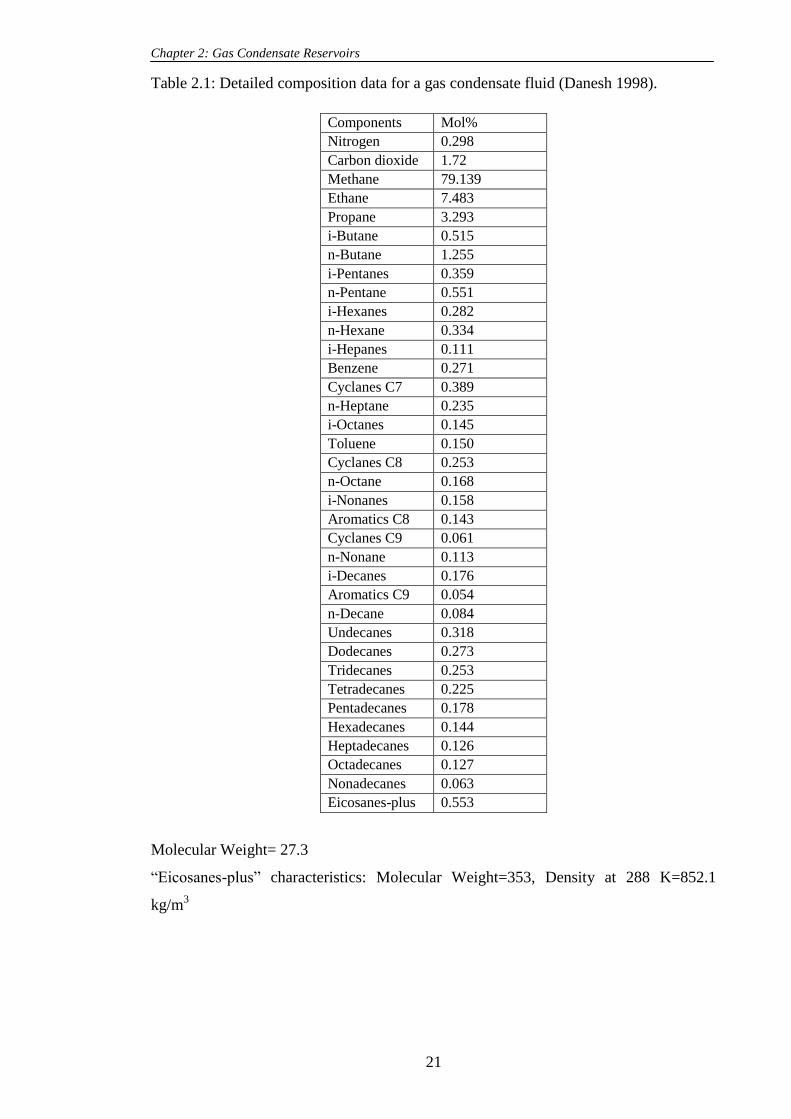
Chapter 2: Gas Condensate Reservoirs
21
Table 2.1: Detailed composition data for a gas condensate fluid (Danesh 1998).
Components Mol%
Nitrogen 0.298
Carbon dioxide 1.72
Methane 79.139
Ethane 7.483
Propane 3.293
i-Butane 0.515
n-Butane 1.255
i-Pentanes 0.359
n-Pentane 0.551
i-Hexanes 0.282
n-Hexane 0.334
i-Hepanes 0.111
Benzene 0.271
Cyclanes C7 0.389
n-Heptane 0.235
i-Octanes 0.145
Toluene 0.150
Cyclanes C8 0.253
n-Octane 0.168
i-Nonanes 0.158
Aromatics C8 0.143
Cyclanes C9 0.061
n-Nonane 0.113
i-Decanes 0.176
Aromatics C9 0.054
n-Decane 0.084
Undecanes 0.318
Dodecanes 0.273
Tridecanes 0.253
Tetradecanes 0.225
Pentadecanes 0.178
Hexadecanes 0.144
Heptadecanes 0.126
Octadecanes 0.127
Nonadecanes 0.063
Eicosanes-plus 0.553
Molecular Weight= 27.3
“Eicosanes-plus” characteristics: Molecular Weight=353, Density at 288 K=852.1
kg/m3

Chapter 2: Gas Condensate Reservoirs
22
Figure 2.1: A phase diagram of a multi component mixture (Danesh et al. 1998).
Figure 2.2: The pressure profile around the wellbore in a gas condensate reservoir
(Danesh et al. 1998).
Black Oil Gas
Gas Condensate

Chapter 2: Gas Condensate Reservoirs
23
(a)
(b)_
Figure 2.3: The phase diagram of two binary mixture reservoir fluids used in the present
study, a) C1-nC4 (C1 73.6%), tres=100 0f b) C1-nC10 (C1 88%), tres=250
0f

Chapter 2: Gas Condensate Reservoirs
24
Figure 2.4: The velocity effect on the gas relative permeability (Final Report of Gas
Condensate Research Group 1999-2002).
Chapter 3: Flow around Horizontal Wells
25
FLOW AROUND HORIZONTAL WELLS
3.1 INTRODUCTION
Over the last few years, many horizontal wells (HWs) have been drilled around the
world. The major purpose of a HW is to enhance reservoir contact and thereby enhance
well productivity. Often, the productivity index of a HW is 3 to 4 times that of a vertical
well (VW) in the same reservoir; as a result several VWs can be replaced by one HW.
However, the main disadvantage of a HW is the cost of drilling and operational risk
which is much more than that for a VW.
The flow behavior around the horizontal wells is more complicated than that for the
vertical wells due to 3-D flow geometry. The flow regime is a combination of linear and
radial flow. Simulating such a complex 3-D flow using numerical commercial
simulators requires the fine grid approach, which is very impractical and cumbersome.
This is especially important for gas condensate reservoirs where the phase change and
velocity dependencies of their relative permeability further complicates the flow
calculation. In gas condensate reservoirs, as the pressure falls below dew point, a bank
of condensate forms around the wellbore, which is affecting the well productivity and
flow behaviour around the wellbore. The flow behaviour is further complicated by the
variation of relative permeability due to the coupling (increase in kr by an increase in
velocity or decrease in IFT) and inertial (a decrease in kr by an increase in velocity)
effects.
This study aims to propose new methodologies to include the impact of geometrical
and flow parameters affecting the performance of a HW in gas condensate reservoirs.
The approach is based on proposing an appropriate expression of skin (or effective
wellbore radius) for an equivalent open hole system of a VW.
3.2 LITERATURE REVIEW
Due to the popularity of drilling HWs, many studies have been conducted to propose
an accurate formulation for productivity of such wells at steady state (SS) or pseudo
steady state (PSS) conditions. However, these are only applicable for single phase
conditions. (Borosiv 1984; Joshi 1985; Giger, 1985, Ronal and Dupuy, 1991, Permadi
1995, Shedid 1996, Economides 1996, Helmy,.and Wattenbarger 1998, Jin Lu 2001,
Furui 2003, Lu and Taib 2007, Helmy, and Wattenbarger 1998, Babu-Odeh 1989 and

Chapter 3: Flow around Horizontal Wells
26
Goode 1991). Theses equations were obtained using semi-mathematical methods and
some simplifying assumptions. Here in this section, the author reviews comprehensively
the previously published works and also the limitation on the application of theses
equations is given.
First equation for HWs productivity calculation at steady state conditions was
presented by Borosiv in 1984. He used potential flow theory to obtain his equation
based on assuming an elliptical shape for a HW drainage area as follows:
w
e
ooHW
r
h
L
h
L
r
Bp
kh
q
2ln
4ln
2
(3.1)
where kh, q and P are the reservoir permeability, flow rate and pressure drawdown in
the reservoir, rw, ehr , L , and h are the wellbore radius, reservoir external radius,
horizontal well length, and reservoir thickness, respectively. o is oil viscosity and oB
is the oil formation volume factor.
It should be noted that the above equation is only applicable for isotropic
formations.
Joshi (1985) developed another equation to calculate the productivity of HWs at
steady state conditions, which is very popular in the petroleum industry. He assumed
that the HW was located in the centre of an elliptical drainage area, Figure 3.1a. He
divided a three-dimensional (3-D) problem into two two-dimensional (2-D) problems,
Figure 3.1b. The 2-D flow of horizontal and vertical planes was calculated using
potential flow theory and an electrical analogy concept. The derived equation is based
on the uniform flux distribution along the wellbore. Joshi‟s equation is expressed as
follows:
w
ooHW
r
h
L
h
L
Laa
Bp
kh
q
2ln
2
2ln
2
2
2
, (3.2)
where
4
5.0
1
4
1
2
1
2
er
L
La . (3.3)

Chapter 3: Flow around Horizontal Wells
27
The above equation is also only applicable for calculation of HW productivity in an
isotropic formation. For an anisotropic formation, he adapted Muskat‟s vertical axis
transformation (v
h
kk
hz ' ) and proposed a different equation as follows:
v
h
kk
hz ' , (3.4)
w
aniani
ooHW
r
hI
L
hI
L
Laa
Bp
kh
q
2ln
2
2ln
2
2
2
. (3.5)
where
v
hani k
kI . (3.6)
where vk and hk are vertical and horizontal well permeability.
It should be noted that Joshi ignored the effect of the vertical z-direction
transformation on the wellbore radius.
He also developed the following equation to account for the effect of the wellbore
location in the perpendicular axis (Z) using Muskat‟s off-centred wells formulation:
w
ooHW
r
lh
L
h
L
Laa
Bp
kh
q
2
2ln
2
2ln
2
22
2
2
. (3.7)
l is the distance of the HW wellbore from middle of the reservoir thickness.
The HW productivity can also be expressed using the VW productivity with a
geometric skin factor.
m
w
e
HW
Sr
r
Pkhq
ln
2
(3.8)
Sm is the geometric skin and re is the exterior radius of the reservoir model, which
for a square drainage area can be calculated as follows:
res
e
Xr . (3.9)
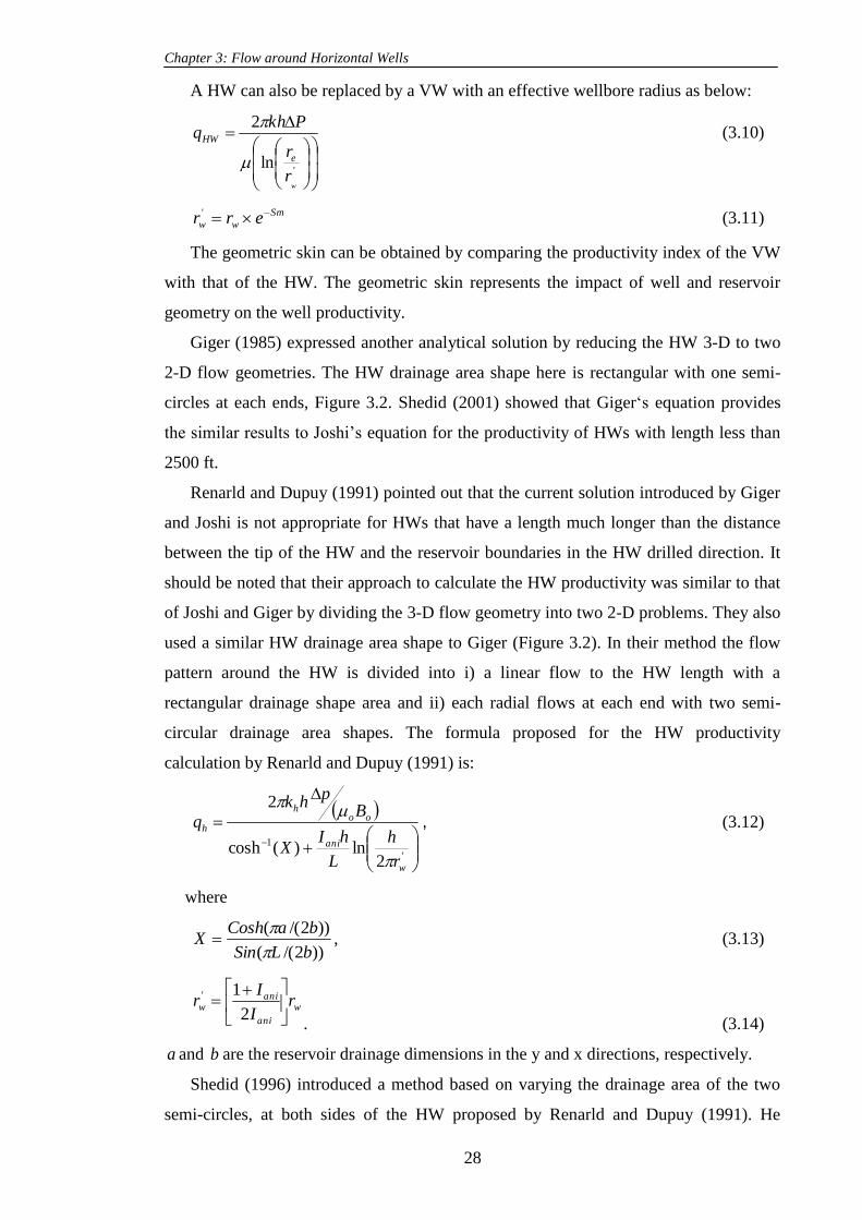
Chapter 3: Flow around Horizontal Wells
28
A HW can also be replaced by a VW with an effective wellbore radius as below:
'ln
2
wr
r
Pkhq
e
HW
(3.10)
Sm
ww err ' (3.11)
The geometric skin can be obtained by comparing the productivity index of the VW
with that of the HW. The geometric skin represents the impact of well and reservoir
geometry on the well productivity.
Giger (1985) expressed another analytical solution by reducing the HW 3-D to two
2-D flow geometries. The HW drainage area shape here is rectangular with one semi-
circles at each ends, Figure 3.2. Shedid (2001) showed that Giger„s equation provides
the similar results to Joshi‟s equation for the productivity of HWs with length less than
2500 ft.
Renarld and Dupuy (1991) pointed out that the current solution introduced by Giger
and Joshi is not appropriate for HWs that have a length much longer than the distance
between the tip of the HW and the reservoir boundaries in the HW drilled direction. It
should be noted that their approach to calculate the HW productivity was similar to that
of Joshi and Giger by dividing the 3-D flow geometry into two 2-D problems. They also
used a similar HW drainage area shape to Giger (Figure 3.2). In their method the flow
pattern around the HW is divided into i) a linear flow to the HW length with a
rectangular drainage shape area and ii) each radial flows at each end with two semi-
circular drainage area shapes. The formula proposed for the HW productivity
calculation by Renarld and Dupuy (1991) is:
'
1
2ln)(cosh
2
w
ani
ooh
h
r
h
L
hIX
Bp
hk
q
, (3.12)
where
))2/((
))2/((
bLSin
baCoshX
, (3.13)
w
ani
aniw r
I
Ir
2
1'
. (3.14)
a and b are the reservoir drainage dimensions in the y and x directions, respectively.
Shedid (1996) introduced a method based on varying the drainage area of the two
semi-circles, at both sides of the HW proposed by Renarld and Dupuy (1991). He

Chapter 3: Flow around Horizontal Wells
29
divided the HW‟s drainage area into three parts, i) a rectangular area with length L ii) a
small rectangle of length rL/C at the heel side, constant C is calculated by matching the
results of the flow rates calculated for the heel-end of HW and the corresponding values
of Borosiv and Joshi‟s equation and iii) a semi-circle of radius r at the toe-end. The
analogy between Darcy and Ohm‟s equation was used to obtain the flow resistance for
each part. His formula is expressed as follows:
hrL
C
hL
rh
Bp
hk
q
w
w
ooh
h21
25.02ln
2
. (3.15)
His formulation is only valid for calculating the HW productivity in isotropic
formations.
It was well documented that the HWs productivity decreases significantly by
decreasing anisotropy. As mentioned earlier, above equations were obtained based on
assumption of the isotropic formation and then as explained before they adopted for
anisotropic formation. That is, the application of these equations in the anisotropic
formations is always questionable. It will be discussed later this was a topic of many
researchers which their work was to give a better formulation for the HWs productivity
in the anisotropic formations.
Later a simulator based on finite volume was developed by Economides et al. (1996)
to study the well productivity of HWs in anisotropic reservoirs. They used local grid
refinement to capture the complexity of flow around HWs. They also compared their
simulation results with the corresponding values obtained using Joshi‟s equation. They
reported a significant difference between these two results. They also concluded that
Joshi‟s equation may not predict HW productivity accurately specially for anisotropic
reservoirs. They applied the effect of anisotropy on the wellbore radius and on the
reservoir thickness using the Peaceman‟s equation and Muskat‟s transformation on
Joshi‟s equation (3.2) as follows:
)1(ln
2
2ln
2
2
2
aniw
aniani
ooh
Ir
hI
L
hI
L
Laa
Bp
kh
q
. (3.16)
As was discussed by Sheng (2007), the solution for an anisotropic problem can not
be obtained directly by transforming it into an isotropic system. The flow geometry

Chapter 3: Flow around Horizontal Wells
30
around the wellbore is highly complex and there are a lot of factors which may need to
be taken into account.
Lu (2001) developed an equation based on a solution to this 3-D problem obtained
using fluid potential theory. This approach was similar to that followed by Joshi and
Giger but assumed that the HW is in a very large drainage area, so the pressure
distribution has not met the reservoir boundary during production time. He
demonstrated that there are significant differences between the results obtained using
this equation and Joshi and Borosiv‟s equations for some cases.
In 2003, Furi et al. developed a semi-analytical model to evaluate the formation
damage around the HW including reservoir anisotropy and damage heterogeneity. He
also derived an inflow equation for HW based on dividing the flow into two regions.
The first flow region has a cylindrical shape around the HW, i.e. it is a radial flow
pattern with a radius of2
2h . The linear flow region, the second region, starts from the
end of the first region and continues to the reservoir boundary. The formula for pressure
drop is expressed as summation of the pressure drop in these two regions.
Wange et al. (2007) presented another equation to predict the productivity of the
HW. In his model, the flow geometry around the HW is described by dividing the
reservoir thickness into three parts. These parts consist of three rectangular box- shaped
sections with a thickness of wrh
2, wr2 and wr
h 2
. It was assumed that the flow to the
second part is purely horizontal while the first and third parts have horizontal and
vertical elements. Their proposed formula for HW productivity includes the wellbore
eccentric (location) effects. They concluded that Joshi‟s equation does not apply to
HWs which are not located at the mid point.
Shedid (2001) conducted a series of sensitivity studies to estimate the flow rate for
HWs using steady state equations proposed by other investigators mentioned above
(Joshi, Giger, Borosiv, Renarld and Dupuy, Permadi and Shedid (1996)). He concluded
that these equations provided similar values for HW productivity for a HW length less
than 1000 ft. For the HWs with the length of over 1000 ft, Joshi and Borosiv„s
equations still provided similar results. However the productivity of HWs calculated
using the rest of equations of the other researchers were significantly different. His
results also confirmed that the relative advantages of HWs to VWs are decreased as the
reservoir thickness increases. Thus the use of HWs is predominantly recommended for
reservoirs with thin formations. Humberto (2008) also conducted a series of similar
sensitive studies and came to the same conclusion. He also proposed another equation,

Chapter 3: Flow around Horizontal Wells
31
which is a combination of the Joshi and Renarld„s equations using some weight
coefficients, which were determined using a trial and error procedure by comparing
them with his numerical simulation results.
The aforementioned equations can be applied for a single-phase flow,
incompressible fluid at steady state conditions.
Many investigators (Economides 1996, Helmy and Wattenbarger 1998, Lu, and
Tiab 2007) studied the HW single phase productivity index (PI) under pseudo steady
state (PSS) conditions. In the case of PSS flow, where the pressure gradient within the
reservoir, with constant pressure at the outer boundary, drops at the same rate, it is
necessary to solve the diffusivity equation. Solving the diffusivity equation for the 3-D
HW geometry analytically is a complex task; therefore there are a number of
oversimplifying assumptions for the HW flow geometry in these approaches. Among
them, the HW PI equations introduced by Babu-Odeh (1989) and Goode (1991) are
more popular than others. These equations were derived by developing a semi analytical
solution to the PSS pressure drop of a HW in the centre of a box shaped drainage area.
The PSS model presented by Babu -Odeh (1989) used the uniform flux distribution
assumption along the wellbore (constant rate), whilst Goode (1991) made the
assumption of uniform (constant pressure) wellbore pressure along the wellbore. These
equations are quite complicated and require intensive calculations, which can be
facilitated partly by developing an appropriate computer code. The former, Babu-Odeh
„s equation, is easier to use than the latter, which involves more complex infinite series
in the HW PI expression, but it is less accurate. Economides (1996) pointed out that
there are differences between the predicted HW productivity indexes using these
equations. However, these differences decrease as the partial penetration increases.
Kamkom and Zhu (2006) presented the IPR (Inflow Performance Relationship)
equation for horizontal gas wells. Their equation was obtained simply by converting the
IPR equation for oil wells to gas wells by using Boyles Law. However this is limited to
a single phase and is not applicable to gas condensate reservoirs.
There are only a few sensitivity studies, which have discussed the application and
productivity of the HWs in gas condensate reservoirs. Hashemi et al. (2005) conducted
a series of sensitivity studies to compare the well productivity of horizontal,
hydraulically fractured and VWs in a lean gas condensate reservoir. Their results
showed that the HW improve productivity significantly when the bottom hole pressure
is below dew point. Numerical simulations (Dehane 2000, Boualem 2006 and
Jamiolahmady et al. 2007) conducted on the HWs have mainly been focused on the

Chapter 3: Flow around Horizontal Wells
32
sensitivity of pertinent parameters on the performance of such wells. Therefore an
equation and a methodology for estimation of well productivity of HWs in gas
condensate reservoirs are required, as proposed in this study.
This study is divided into three parts. The first part is devoted to conducting a series
of sensitivity analyses evaluating the impact of pertinent parameters, including reservoir
thickness, layering, anisotropy, fluid richness, condensate liquid drop out, coupling and
inertia on the efficiency of a single HW model using ECLIPSE300. Difficulties faced
with using the commercial reservoir simulators will be also discussed during this
exercise. This is one of the reasons that the author developed in-house simulators to
study the flow behaviour around HWs in gas condensate reservoirs.
In the second part, in a systematic mathematical modelling approach, the flow of a
single-phase around a HW has been simulated. The integrity of the simulator has been
confirmed by comparing some of its results with those of the ECLIPSE. It is
demonstrated that the anisotropy has a significant effect on HW productivity, when
kv/kh is less than 0.6. To capture the anisotropy effect accurately, a very fine grid is
required using commercial reservoir simulators. The limitations of Joshi, Joshi-
Economides semi-analytical skin expressions for anisotropic formation are also
examined.
Next, based on the results of the in-house simulator, a geometric skin correlation
developed for an undamaged formation penetrated by a HW is presented. In this
exercise the efficient statistical response surface method has been used. This approach
will be briefly described in a separate section (section 6).
The accuracy of the geometric skin formulation has also been confirmed by
comparing its prediction for the data points not used in its development and also the
predictions of some of the semi-analytical formulations described above.
The effect of partial penetration on the productivity ratio (PR) and geometric skin
have also been studied extensively.
For the non-Darcy flow system, where the flow performance at high velocity is
negatively affected by the inertia, an effective wellbore radius formulation has been
developed, based on the results of the developed simulator. The proposed equation
benefits from suitable dimensionless numbers which express the impact of pertinent
parameters, i.e. velocity and geometric parameters.
As discussed earlier, the formulations available in the literature are for single phase
Darcy flow. In gas condensate reservoirs, the flow behaviour around HWs is more
complex due to the combined effect of coupling and inertia. Gas condensate fluid also
Chapter 3: Flow around Horizontal Wells
33
involves complex thermodynamic behaviour, due to fluid compositions. A fully
compositional modelling is required to predict accurately the well performance of HWs
in gas condensate reservoirs. Therefore, in line with the objectives of this study, this
part is devoted to mathematical modelling of gas condensate flow around the HWs. A
two phase compositional simulator has been developed, which incorporates new
generalised krgtr correlation (Jamiolahmady et al. 2009). This correlation accounts for
the combined effect of inertia and coupling with universal parameters. The integrity of
the simulator has been confirmed by comparing its results with the results of the
ECLIPSE commercial reservoir simulator under the same flowing conditions. Next, a
comprehensive sensitive study has also been conducted to evaluate the impact of
pertinent parameters on the performance of HWs in gas condensate reservoirs.
The second part of this study is devoted to developing a methodology for prediction
of the well productivity of HWs in gas condensate reservoirs. Here the effective
wellbore radius approach mentioned above is extended from single phase non-Darcy
flow to a two-phase flow of gas and condensate. The integrity of the proposed method
has been confirmed by comparing the results of the developed 1-D open hole
compositional in-house simulator with the effective wellbore radius with the
corresponding values obtained using the 3-D HW compositional simulator.
Finally, an in-house simulator is introduced that has been developed to study the
flow behaviour of single phase gas around HWs at pseudo steady state conditions. The
results of the in-house simulator are shown to be in good agreement with the
corresponding values obtained for a fine grid model created using ECLIPSE. The
applicability of the methodology, initially proposed for steady state conditions, to
pseudo steady state conditions has been investigated comprehensively. This study
demonstrates that the proposed methodology is general and can be used as a standard
technique for steady state, pseudo steady state and transient state conditions. An
equivalent phase approach has also been proposed to model two phase flow of gas
condensate for pseudo steady condition. A two phase 3-D HW and 1-D EOH in-house
simulator has been developed to verify the accuracy of the proposed formulation and
approach for pseudo steady conditions.
3.3 GAS-CONDENSATE HW MODEL, ECLIPSE 300
In this part of the study, the single well model constructed in ECLIPSE300 is used
to evaluate the impact of pertinent parameters including the HW length and the

Chapter 3: Flow around Horizontal Wells
34
reservoir thickness on the gas condensate HW productivity. The model will then be
used to examine the effects of inertia and coupling.
3.3.1 Effect of HW Length and Reservoir Thickness
The aim of this exercise is to quantify the impact of the HW length and reservoir
thickness on the total gas production of a gas condensate HW.
Reservoir Modelling
Here, a single well model was constructed using ECLIPSE300 with a 3-D Cartesian
fine grid system. The reservoir model is a homogenous reservoir model. The core
properties are those of Texas Cream core used in the laboratory of a research gas
condensate project. The basic properties of the core samples used in this study are found
in Table 3.1. The core specific constants of the velocity dependent relative permeability
correlations in ECLIPSE 300 were those experimentally measured on these cores in this
laboratory. The pseudo-pressure option of ECLIPSE 300 has been used to account for
positive coupling and negative inertial effects around the wellbore. The reservoir
dimensions for a set of sensitivity studies are those listed in Table 3.2 for a model
referred to as model A. The initial reservoir pressure was above dew point of the
reservoir fluid. However the bottom hole pressure was kept below the reservoir fluid
dew point, which created a two phase gas and condensate region around the wellbore.
The initial gas production plateau rate is maintained at 50 Mscf for all runs till the
bottom hole pressure approaches 4400 psi, which is below the dew point. For all
models used here the effect of pressure drop inside the HWs due to the friction on the
HW productivity was ignored.
Fluid Properties
Three C1-nC10 gas condensate binary model fluids with 7, 16 and 30% v/v,
maximum liquid dropout (MLDO) in the constant composition expansion (CCE) test at
the reservoir temperature of 250oF were used in this study. The corresponding dew
point pressure values were 4132, 5180 and 5405 psia, respectively. In ECLIPSE 300 the
Lorentz Bray Clark viscosity correlation and Peng Robinson equation of the state were
used to estimate the corresponding fluid properties. In the majority of the simulations
conducted here, a fluid system with intermediate richness was used unless otherwise
stated.

Chapter 3: Flow around Horizontal Wells
35
Results & Discussion:
Many simulation runs were performed for different HW lengths varying from 700 to
3100 ft in a reservoir with the thickness of 50, 100, and 200 ft. As the model is
symmetrical in a Cartesian system, in order to reduce computing time for these
simulations, only half of the model has been selected.
As expected, increasing the length of the HW improved well productivity, although
as the length increased, the extra benefit diminished. For example, a 35% increase in the
length (from 1150 to 1550 ft) would increase the total production by only 0.48 %, while
increasing the HW length from 350 to 472 ft (35% increase in the length) increases the
total production by 1.5%, Figure 3.3. It is also noted that the gas recovery is always
achieved faster using the HW compared to that of the VW in the reservoir.
Figure 3.4 shows the relative increase in cumulative gas production for the HW
compared to that of the VW versus time for three reservoir models with a thickness of
50, 100 and 200 ft. In the case of a HW length of 350 ft, the relative increase in
cumulative gas production amounts to maxima of 33%, 18%, and 11% for the reservoir
with 50, 100, and 200 ft thickness while the corresponding values for the HW length of
1550 ft are 95%, 52%, and 27%, respectively. It is concluded that increasing the
thickness of the reservoir decreases the relative gain in the total gas production
compared to that of a VW. Increasing the length of the horizontal section from 350 to
1550 ft in the reservoir 50 ft thick increased the relative gain in the total gas production
compared to that of a VW from 33% to 95%, while the corresponding value in the
reservoir 200 ft thick increased only from 11% to 27%. It is concluded that the effect of
the length of the horizontal section on the total gas productivity is more pronounced in
the case of the reservoirs with smaller thicknesses.
3.3.2 Effect of Inertia and Coupling
This part of the study attempts to quantify the effect of inertia and coupling, fluid
richness and rock properties on gas condensate HW performance.
Reservoir Modelling
The reservoir dimensions are those listed in Table 3.2 for a case referred to as Model
B. All runs were made for a period of one years‟ production with the bottom hole
pressure at 4000 psi and the initial reservoir pressure at 7500 psi. The single layer
reservoir model properties were described by Texas Cream properties, Table 3.1.

Chapter 3: Flow around Horizontal Wells
36
Fluid Properties
The reservoir fluid is a binary mixture of C1-C10 with maximum liquid dropout
16% (moderate condensate).
Results & Discussion
Figure 3.5 compares the total gas production for a HW with a length of 100 ft for the
case with and without the inertial and coupling effects and also with only the inertial
effect being active. It should be noted that when velocity effects (i.e. both coupling and
inertia) are ignored for the HW with 100 ft, there is minimal difference in total gas
production, compared to the case where velocity effects are considered, Figure 3.5.
However the total gas production decreased considerably if only the inertial effect is
applied on the model. This demonstrates that the positive coupling effect compensates
the negative impact of inertia on the gas production. The effect of coupling becomes
even more pronounced as the length of HW increased, Figures 3.6 to 3.8. It is important
to point out that the negative inertial effect reduced due to decreasing velocity. It is also
worth mentioning that decreasing or increasing the bottom hole pressure resulted in a lot
of numerical convergence problems for many cases, which could not be removed
despite the considerable efforts of the author.
From Figures 3.9 and 3.10, the same conclusion can be drawn for the reservoir
model described by the Berea core properties, Table 3.1. It should be noted that all the
reservoir model characteristics here e.g. reservoir fluid, grid cells sizes, HW length,
wellbore radius and the pressure drop across the reservoir model were the same as those
used for the former one. However, many convergence problems were experienced for
the HW longer than 500 ft, which is why the reported results here are only for the HWs
with a length less than 500 ft.
For the last series of simulations, the reservoir model properties were described by
RC1b properties, Table 3.1. As the inertial effect reduces due to the decreased velocity
of this tight rock, the coupling effect becomes more dominant, improving the gas
production significantly, Figures 3.11 to 3.14. It is obvious that the velocity and IFT
determine the impact of coupling or inertia.
It should be pointed out that drilling of a HW in a gas condensate reservoir,
similarly to that in a dry gas reservoir, decreases the negative impact of the inertia, due
to decreasing the velocity. However, the pronounced effect of the coupling in the former
also improves the total gas production.

Chapter 3: Flow around Horizontal Wells
37
It is important to note that due to numerical instability problems, none of the above
runs converged when the reservoir fluid is a rich gas.
In summary, as mentioned previously, the main difficulty in modelling gas
condensate flow around HWs is the complexity of the flow behaviour around the
wellbore for these low IFT systems. Significant effort was directed to simulate gas
condensate flow around HWs using ECLIPSE 300 under different flow conditions. The
results of this exercise concluded that:
1) The flow around HWs is very complex and requires a full 3-D compositional
approach to describe it accurately. However, it does not provide accurate
results around the wellbore unless an extremely fine grid is used, which is
costly and cumbersome.
2) Furthermore, performing this exercise using commercial compositional
simulators results in convergence problems due to numerical instability. An
increase in the length of HW increases numerical convergence problems.
The problem of convergences is more severe in the cases of using moderate
and rich gas condensate fluid systems. It should be noticed that the reservoir
fluid here was a binary mixture (C1-C10), but in reality the number of
components of the typical gas condensate reservoir is much greater than two.
This makes the calculation procedure more complicated for most practical
cases. Furthermore the implicit computing and iteration nature of the
calculations require much longer CPU times.
3) The velocity dependent kr formulations (Henderson et al. 2000) are available
in ECLIPSE not the new more efficient generalised kr correlation
(Jamiolahmady et al. 2009). The former has separate formulae to take
account of the effects of inertia and coupling requiring core specific
constants. This correlation would not be able to acknowledge the impact of
coupling and inertia for a wide range of velocity and IFT.
To this end, a reliable approach, which tackles all uncertainty associated with the
well performance of gas condensate HWs is desirable. The author therefore embarked
on a modelling approach, different from that using the commercial simulators, and
developed different mathematical simulators using Comsol multi-physics mathematical
package, which is based on finite-element methods. In a systematic approach, first the
flow of a single-phase around a HW was simulated. Then it was extended to two phase
flow of the gas and condensate fluids as described below.

Chapter 3: Flow around Horizontal Wells
38
3.4 SINGLE PHASE HW MODEL, ISOTROPIC FORMATION
At this stage of the study, the flow of a single-phase compressible fluid around the
wellbore of a HW has been simulated. As mentioned earlier, the main objective of this
study is to expand the mathematical modelling approach to two phase flow of gas
condensate fluids.
It should be noticed that the current developed single phase flow in-house simulator
has an option to account for the change in fluid properties with pressure and the effects
of inertia. Initially, these effects have been ignored to develop a geometric skin for
HWs, which is independent of flow rate and fluid properties. Next flow skin, which
accounts for the effects of a change in fluid properties with pressure and non-Darcy
flow, is studied.
This part of the study consists of two sections. The first section describes the in-
house simulator. Next the integrity of the 3-D HW in-house simulator is confirmed by
comparing some of its results with those of the same HW constructed by the ECLIPSE
simulator.
3.4.1 In-House Mathematical Single Phase HW Model
The main aim of the present study is to develop a 3-D simulator that can be used for
creating a large bank of data for HWs with different lengths and wellbore radii in a
reservoir with different dimensions and thicknesses.
The 3-D system considered in this study consists of a HW with radius of rw and
length of L, in a single layer cubic reservoir, as shown in Figure 3.15. This homogenous
porous medium has an absolute permeability k and formation thickness of h. The length
of the reservoir in the x and y directions is assumed to be 2.5 times the length of the
HW. Later in this chapter, it will be shown that the impact of partial penetration on the
productivity of HWs and geometric skin for Xres/L>1.5 is negligible.
Due to the existing symmetry only a quarter of the model has been considered in
this study. This saves the computation time and reduces the complexity of having a high
quality mesh. This later point is discussed further in the next section.
Governing Equations
The equations employed in this study are similar to those described for gas
condensate flow in a perforated region (Jamiolahmady et al. 2006). These equations are:
1) Continuity equation for a compressible fluid
0. v . (3.17)

Chapter 3: Flow around Horizontal Wells
39
2) The 3-D form of the Forchheimer equation is:
VVVk
P
. (3.18)
Combining continuity and the 3-D form of the Forchheimer equation, after some
mathematical manipulation, gives:
0
411
.2.2
Pk
Pk
. (3.19)
Mathematical Solution Technique
The governing non-linear partial differential equation (PDE), Equation 3.19, is
solved using Comsol multi-physic software (version 3.4, 2007), which uses the finite
element method. The main dependent variable in this equation is P (pressure).
The boundary conditions applied to this system are:
1) Infinite conductivity for the wellbore (the pressure gradient in the wellbore has
been ignored),
2) The pressure at outer boundary (external radius) is known,
3) The pressure at the inner boundary (wellbore radius) is known.
Initially an attempt was made to construct a full 3-D single HW in a rectangular
reservoir model using options available in the composite toolbar of Comsol user
interface. It should be mentioned that there is a significant difference in the dimensions
of different parts of the reservoir models, e.g. the wellbore radius, the HW length and
the reservoir dimensions. This caused considerable difficulties when creating the mesh
geometry, in some cases, it was even impossible. Significant efforts were dedicated to
improving the procedure. It was concluded that the construction of such a 3-D object is
not feasible for most cases considered. It is well known that creating 2-D or 1-D
geometry is simpler than 3-D geometry. Therefore, the author has benefited from the
symmetry of the system and initially created a 2-D geometry which was then extruded
to a complete 3-D system. This method proved very efficient in removing all the
problems associated with directly constructing the 3-D HW model. The important point
here is that adding and subtracting regions to create the complicated geometry under
study has been performed in the 2-D plane of the geometry.
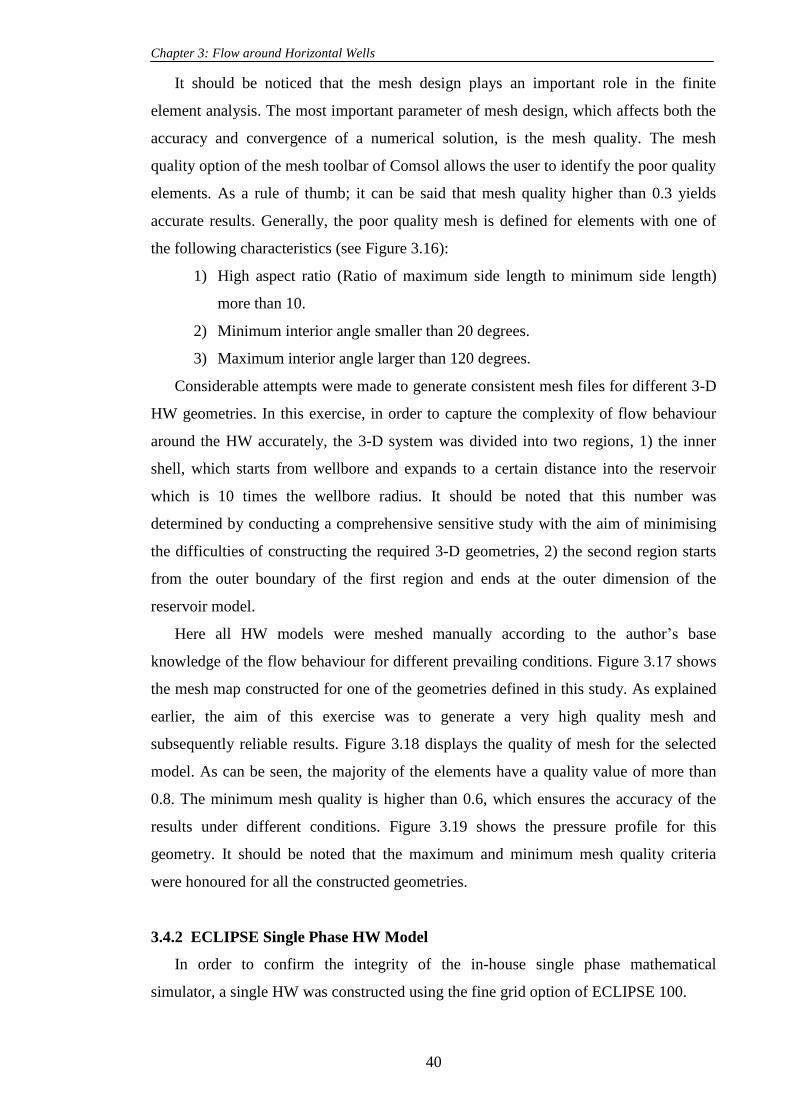
Chapter 3: Flow around Horizontal Wells
40
It should be noticed that the mesh design plays an important role in the finite
element analysis. The most important parameter of mesh design, which affects both the
accuracy and convergence of a numerical solution, is the mesh quality. The mesh
quality option of the mesh toolbar of Comsol allows the user to identify the poor quality
elements. As a rule of thumb; it can be said that mesh quality higher than 0.3 yields
accurate results. Generally, the poor quality mesh is defined for elements with one of
the following characteristics (see Figure 3.16):
1) High aspect ratio (Ratio of maximum side length to minimum side length)
more than 10.
2) Minimum interior angle smaller than 20 degrees.
3) Maximum interior angle larger than 120 degrees.
Considerable attempts were made to generate consistent mesh files for different 3-D
HW geometries. In this exercise, in order to capture the complexity of flow behaviour
around the HW accurately, the 3-D system was divided into two regions, 1) the inner
shell, which starts from wellbore and expands to a certain distance into the reservoir
which is 10 times the wellbore radius. It should be noted that this number was
determined by conducting a comprehensive sensitive study with the aim of minimising
the difficulties of constructing the required 3-D geometries, 2) the second region starts
from the outer boundary of the first region and ends at the outer dimension of the
reservoir model.
Here all HW models were meshed manually according to the author‟s base
knowledge of the flow behaviour for different prevailing conditions. Figure 3.17 shows
the mesh map constructed for one of the geometries defined in this study. As explained
earlier, the aim of this exercise was to generate a very high quality mesh and
subsequently reliable results. Figure 3.18 displays the quality of mesh for the selected
model. As can be seen, the majority of the elements have a quality value of more than
0.8. The minimum mesh quality is higher than 0.6, which ensures the accuracy of the
results under different conditions. Figure 3.19 shows the pressure profile for this
geometry. It should be noted that the maximum and minimum mesh quality criteria
were honoured for all the constructed geometries.
3.4.2 ECLIPSE Single Phase HW Model
In order to confirm the integrity of the in-house single phase mathematical
simulator, a single HW was constructed using the fine grid option of ECLIPSE 100.

Chapter 3: Flow around Horizontal Wells
41
The core properties of Texas Cream (Table 3.1) with porosity 0.21 and permeability
11.1 mD were used to describe the reservoir in this model. The PVT tables were set up
based on information from the study of flow around perforated region by Jamiolahmady
et al. (2007). That is, single phase gas with specific gravity of 0.7, viscosity of 0.0352
cp and the formation volume factor of 0.0103 Rm3/Sm
3. The reservoir was 250 m in the
x and 125 m in y directions and 16 m in the Z direction. The length of HW was 100 m.
The reservoir pressure was 82.737 bar and the HW was producing with a controlled
bottom hole pressure of 68.9476 bar. Fine grids were used to capture the complexity
flow near the wellbore.
Forty injection wells were located in the boundary of the reservoir to make the
reservoir pressure at the drainage boundary constant.
The results of the in-house mathematical simulator were compared with those of
similar simulations conducted using the ECLIPSE simulator. Figure 3.20 shows the
good agreement between the two results. The arithmetic average absolute percentage
deviations (AAD%) of the predicted mass flow rates values by the ECLIPSE simulator
compared to those estimated by the HW simulator was 1.43 % for the simulation with a
constant pressure drop (P) of 1300 psi maintained over the drainage area. The
corresponding values for a constant pressure drop (P) of 200 and 100 psi were 1.39%
and 0.23%, respectively.
3.5 SINGLE PHASE HW MODEL: ANISTROPIC FORMATION
This study is aimed at investigating the effect of anisotropy on the well performance
of HWs. First the author‟s attempts to refine the ECLIPSE model to improve the
accuracy of the results are discussed. Next, these results are compared with the in-house
simulator outcomes, followed by a comparison between the results of the in-house
simulator and those of Joshi‟s semi-analytical equation. The author has also extended
the study for a high anisotropic case, in which vertical permeability is equal to zero.
This last section includes the simulation of HWs in a thin layer flow model with a
thickness equal to that of the wellbore diameter.
3.5.1 In-house Simulator Versus ECLIPSE
The ECLIPSE model used in this study was the same as the one described in Section
3.3.2 (in terms of the well dimension and reservoir properties). The permeability
anisotropy can be considered in ECLIPSE using the multiplier factor in transmissibility
of grid blocks. When the permeability anisotropy index decreases; a sharp pressure drop

Chapter 3: Flow around Horizontal Wells
42
occurs around the wellbore region in the vertical flow direction. Consequently, a very
fine grid in the perpendicular direction is required to properly model the pressure
distribution around the wellbore.
Figure 3.21 shows the productivity ratio (ratio of flow rates of HW to VW) versus
anisotropy values for the ECLIPSE model using different grid sizes. The results using
three grid sizes show a reduction in estimated flow rate, which is an indication in the
improvement of the accuracy, as the grid is refined. As discussed by Jamiolahmady et
al. (2007), studying flow around a perforated region, an inadequate number of grids and
refinement resulting in an overestimation of flow rate is something also observed here
for coarser grids. An important point noted was that refining more the ECLIPSE model
was not achievable here, due to the high CPU required. It is clear that noticeable
differences between ECLIPSE productivity values from normal and fine grids models
and those calculated by in-house simulator are observed particularly for low anisotropy
values. The extremely fine-grid ECLIPSE model and in-house simulator (with linear
Lagrange element) match very well over a wide range of anisotropy values, although a
clear deviation exists for anisotropy values below than 0.1. The in-house simulator is
more accurate as will be discussed later. It is well known that the strength of the finite
element method technology is its robustness, modularity and reliability (Hughes 1987).
The finite element method is very flexible to cope with complex geometries with
various inner and outer boundary conditions. The finite element method is used to find
an approximation function for the response by dividing domain into finite smaller
subdomains called elements. The shape of the function inside the elements is
determined using an interpolation scheme. The function inside the elements is used to
find an approximation solution for the main domain. This function could be a linear,
quadratic or cubic polynomial. It should be mentioned that there are two techniques
which can be used to enhance the accuracy of the solution. The first, which has been
used in this study, is to keep the polynomial order of element shape function low or
constant, while the mesh is refined by increasing the number of elements. The second
method is to keep the mesh fixed and increase the order of polynomial element function
resulting in the refinement of the solution to obtain the desired convergence and
accuracy (Babus ka et al. 1981, Hughes 1987, Babus ka, and Suri 1990 and Szabo and
Babus ka 1991). Considerable effort was directed to improve the accuracy of the in-
house simulator using a combination of these two major techniques. Mesh refining was
performed, which increased the computational time significantly. It should be noted that
decreasing the anisotropy ratio significantly changes the flow behaviour around the

Chapter 3: Flow around Horizontal Wells
43
HW. It affects the pressure profile counters, making the counter closer near to the
wellbore, i.e. the pressure changes very sharply near the wellbore. Note that the
polynomial shape function element was initially linear. Using higher polynomial order
element shape function (quadratic Lagrange element) and mesh refinement proved to be
effective and efficient to capture these effects for anisotropy values between 0.01 and 1.
However, it was noted that for anisotropies less than 0.01, capturing the sharp changes
in the pressure very close to the wellbore in the z direction proved very difficult. This
was mainly because the large number of mesh elements required for the z-direction
could not be generated. Therefore a new feature (z-scale) was utilised, which allows the
user to generate anisotropic meshes, i.e. more elements lie in the z direction than the
other two directions (x and y). It should be noted that scaling in the z direction for
isotropic formations reduced the accuracy, i.e. the calculated mass flow rates were
overestimated by 9%. Therefore, this was only applied for anisotropic formations. As a
rule of thumb, the z-scale less than 5 can satisfy the required accuracy of the results.
3.5.2 In-house Simulator Versus Joshi (1985), Joshi-Economides (1991) and
Borosiv (1984) Equations
Isotropic Formation
As mentioned previously, many equations have been developed to estimate steady
state flow rate in HWs. Among them, two equations, Equation 3.2 (Joshi 1985) and
Equation 3.1 (Borosiv 1984) are widely used in the petroleum industry.
If these two equations are compared with Equation 3.8 the following geometric skin
expressions are obtained:
w
eh
w
ehm
r
r
r
h
L
h
L
rS ln
2ln
4ln
(3.20)
w
e
w
mr
r
r
h
L
h
L
Laa
S ln2
ln
2
2ln
2
2
(3.21)
Principally, these analytical equations were obtained by simplifying the 3-D system
to two 2-D problems. This assumption is only appropriate if the thickness of the
reservoir model is small compared to the length of HW, that is, the flow is mainly
provided by the HW length compared to the reservoir thickness. Figure 3.22 (a) presents
absolute deviation in percentage (AD%) between the calculated skin values using
Joshi‟s equation (Equation 3.21) and those of the in-house simulator, which were

Chapter 3: Flow around Horizontal Wells
44
calculated using Equation 3.8, and the estimated flow rates by the in-house simulator. It
is noted that when the length of the HW is equal to the thickness of the reservoir, the
gas productivity prediction is poor, using Equation 3.20. However, with increasing
length of the HW, AD% decreases drastically. It seems that Joshi‟s equation provides an
accurate result if L/h is more than 8 for an isotropic formation. In addition, a
comparison of the results of Borosiv‟s Equation (Equation 3.20) with the in-house skin
values shows that Borosiv„s equation gives better results for lower values of L/h
compared to Joshi‟s equation. However, the calculated skin is still significantly
underestimated when L/h is less than 3 (Figure 3.22 (b)).
Anisotropic Formation
The effect of anisotropy on the skin values calculated by the in-house simulator and
those by Joshi (1985) and Joshi-Economides (1996) semi-analytical expressions has
also been examined as described here.
As mentioned earlier, Joshi modified his equation by transforming h to v
h
k
kh to
take into account the reservoir anisotropy (Equation 3.5).
If this equation is compared with radial flow for a VW it gives a geometric skin
formulation expressed by Equation 3.22.
w
e
w
anianim
r
r
r
hI
L
hI
L
Laa
S ln2
ln
2
2ln
2
2
. (3.22)
As mentioned earlier, Economides et al. (1996) modified Joshi‟s equation. If their
proposed formulation (Equation 3.15) is compared with that of radial flow for a VW it
gives a geometric skin formulation expressed by Equation 3.23.
w
e
aniw
anianim
r
r
Ir
hI
L
hI
L
Laa
S ln)1(
ln
2
2ln
2
2
(3.23)
Figure 3.23 and 3.24 compare the calculated skin, for anisotropic formations, using
Joshi‟s (Equation 3.22) and Joshi-Economides‟s (Equation 3.23) equations with the
corresponding values obtained by applying the calculated in-house simulator mass flow

Chapter 3: Flow around Horizontal Wells
45
rates into Equation 3.8. The latter values were calculated using Equation 3.8 and flow
rates estimated by the in-house simulator.
There is a noticeable deviation between the calculated skin values using Joshi and
Joshi-Economides equations with those obtained using Equation 3.8 and flow rates
estimated by the in-house simulator, especially for lower kv/kh and L/h values. When
kv/kh is 0.6, the result of the in-house simulator converges with Joshi (1985) and Joshi-
Economides (1996)„s equations for L/h above 12 (see Figure 3.23 (a)). As discussed
earlier, these semi-analytical equations were developed by dividing the 3-D solution
into two 2-D solutions, which is only valid for the long HWs. It is noted that a decrease
of the anisotropy ratio from 0.6 to 0.4 increases the error between the calculated skin
values using their semi-analytical equations (Joshi and Joshi-Economides) and those of
the in-house simulator (see Figure 3.23 (b)). Figure 3.24 shows that the overestimated
flow rates from these two equations are more pronounced at a lower kvkh of 0.1 and
0.01. However, the skin values from these two Equations and the in-house simulator
results converge for L/h above 25. In summary, the deviations are more pronounced at
lower L/h and lower kv/kh values. In general, it is concluded that the use of these
equations is appropriate for L/h greater than 25. In the next section, the performance of
the in-house simulator when 0vk is compared with a thin layer flow HW model to
further verify the integrity of the in-house simulator.
Thin Layer Flow HW Model
A new model was developed to study flow around HWs when 0vk . In this model
the thickness of the layer is the same as diameter of the wellbore. Figure 3.25a shows a
schematic diagram of the thin layer HW flow model simulated using Comsol. The rock
properties and PVT tables were those used for the HW in-house simulator in Section
3.3.2. The pressure drop across the reservoir drainage area was 100 psi. The thin layer
model can represent one of the HW models described in Section 3.3.2 if kv =0. The
calculated mass flow rate for the thin layer model and that of 3-D model were 0.0068,
and 0.0076 kg/s, respectively. The standard and absolute deviation errors between these
two values are 0.0008 and 10, which confirms the accuracy of HWs in-house simulator.
It should be noted that even with scaling for the HWs in-house simulator, the number of
elements of the thin layer model (557051) is still significantly higher than that of the
HWs in-house simulator with 27386. Figure 3.25b shows the pressure profile across the
HWs in-house simulator. As can be seen, the 3-D HWs in-house simulator with kv=0,
has predicted a pressure profile similar to that of the thin layer model, i.e. fluid flows

Chapter 3: Flow around Horizontal Wells
46
horizontally in a plate with thickness equal to the HW diameter. It was mentioned
previously that z-scale and quadratic Lagrange significantly improved the results of the
in-house simulator especially for anisotropy values above 0.001, Figures 3.21 (b) to
3.25, considering that it is unlikely to drill a HW in the formation with kv=0. The use of
results of the in-house simulator for development of a new and more efficient geometric
skin has been limited to formations with anisotropy values varying between 0.001-1.0.
It should also be mentioned that the equations widely used in the petroleum industry
incorrectly predict zero flow rates for the kv=0 condition according to their .
3.6 RESPONSE SURFACE METHODOLOGY
To develop a more general skin formulation, the author used the response surface
method. It was introduced by Myers and Montgomery (1995) as a statistical tool to
simulate a physical phenomenon in the range of its pertinent parameters. In this method,
the response (quality characteristic or performance measure) is usually a nonlinear
function of several input variables. Typically, the approximation function that relates
structural responses and design variables (important factors which affect the response),
is a polynomial. The most used polynomial approximation surface fit is a quadratic
multidimensional polynomial. The response surface for such cases is described as
follows:
iiiijiijii xaxxaxaay 0 (3.24)
The least square method is used to estimate the constant and coefficients of this
function at certain sample points. In this statistical method, each variable is scaled such
that it varies between 0 and 1. The distribution of a scaled variable is carefully defined
within its maximum and minimum values by a number of nodes and based on a design
criterion. Various techniques, referred to as experimental designs, have been developed
to select sample points. The common experimental design is 2-level factorial, which
includes the upper and lower limits for the variables involved. For this experimental
design, 2k runs are needed, where k is the number of variables or factors. The sampling
points are selected in the r range, where r& are the vectors of mean and
standard variation of the variables, respectively.
3.7 SINGLE PHASE DARCY FLOW
3.7.1 Geometric skin Correlation

Chapter 3: Flow around Horizontal Wells
47
In this part of the study a correlation for a geometric skin is proposed. The
geometric skin, which accounts for the impact of HW geometry on the flow, is
employed in an open-hole VW productivity equation ,giving the same flow rate as that
of the HW as expressed by Equation 3.8. The in-house simulator was used to create a
large bank of experimental data. Using these data, the coefficients of the skin
formulation are determined through a multi-regression exercise.
The main geometrical parameters that influence Sm of HWs are thickness of the
reservoir, radius of the well, length of the HW. To obtain the relevant dimensionless
numbers to be included in the formulations, the author looked at a special case for
which a mathematical expression can be derived as described below.
As can be seen in Figure 3.26, the flow behaviour around a fully penetrating HW is
similar to that around a VW with a circular drainage area and radius h/2. Consequently,
the flow rate of a fully penetrating HW with length of L can be written as follows:
)2/(
2
w
hrhLn
pkLQ
(3.25)
Comparing Equations 3.25 and 3.8 gives the Sm formulation for this system as
expressed by Equation 3.26.
)()2
(w
e
w
mr
rLn
r
hLn
L
hS . (3.26)
Therefore, it is suggested that geometric skin in an isotropic reservoir could be a
linear function of )2
(wr
hLn
L
h, )
2(
wr
hLn and )(
w
e
r
rLn parameters.
))2
(),(),2
((ww
e
w
mr
hLn
r
rLn
r
hLn
L
hfS . (3.27)
As discussed earlier, the well productivity of HWs is greatly affected by anisotropy.
Thus, for an anisotropic reservoir, one can write:
)),2
(),(),2
(( '
aniI
r
hLn
r
rLn
r
hLn
L
hfS
ww
e
w
m .
h
v
k
kI
ani' , (3.28)
where vk and hk are vertical and horizontal permeability, respectively.
Furthermore, to account for the anisotropy effect, according to Muskat„s
transformation, the vertical axis can be modified by:
'
aniI
hh , (3.29)

Chapter 3: Flow around Horizontal Wells
48
Thus the first parameter in Equation 3.28 is replaced by:
)2
ln(''
1
anianiIr
h
IL
hx
w
. (3.30)
Further sensitivity analysis showed that transformation of the vertical axis for the
third parameter decreased the accuracy of the fitting model and using natural log of Iani
rather than Iani proved to give a better fit. Therefore, Sm has been suggested to be a
function of )2
ln(''
anianiIr
h
IL
h
w
, )ln(w
e
r
r, )
2ln(
wr
h and )ln( '
aniI .
))ln(),2
ln(),ln(),2
ln(( '
'' ani
aniani
Ir
h
r
r
Ir
h
IL
hfS
ww
e
w
m . (3.31)
Selection of these dimensionless numbers proved suitable in obtaining an efficient
skin formulation. It is also worth noting that LX res 5.2 and the effect of partial
penetration is discussed separately in the following sections.
The quadratic Response Surface model was chosen as described by Equation 3.32.
4
1
4
1
4
1
24
1
0
i ij
jiij
i
iii
i
iim xxaxaxaaS . (3.32)
More than 600 simulations runs were performed to ensure adequate resolution of
pertinent parameters, based on the 2k factorial experimental design criterion. The
proposed dimensionless numbers were scaled according to the following equation:
minmax
minmax )2(
ii
iii
icxx
xxxx
, (3.33)
where icx is the scaled coded parameter (expressing the impact of reservoir and well
parameters) and maxix and minix are the maximum and minimum of each parameters,
respectively. The maximum and minimum values of the parameters were selected based
on the parameter distribution within their practical range of applications. The
corresponding variables and their range of variations in this study, representing these
three parameters, are shown in Tables 3.3 and 3.4.
Table 3.5 gives the coefficients, upper and lower limits and standard error of the
coefficients of Equation 3.32. The standard error coefficient is used to determine how a
selected parameter is statistically significant. As a rule of thumb, if the value of the
coefficient and its standard error are in the same order of magnitude, the estimated
parameter is not statistically considerable. Here, the results in Table 3.5 indicate that the
chosen parameters are appropriate. Generally the coefficient of multiple determination
(R2) is used to evaluate the accuracy of the fitted model. If the coefficient of multiple

Chapter 3: Flow around Horizontal Wells
49
determination is 1, it provides an excellent response to the input parameters and if the
residual error increases, the multiple determination coefficient reduces in the range of 1
to 0. For the fitted model, the coefficient of multiple determination was 0.9996, which is
satisfactory.
3.7.2 Verification of Geometric skin Formulation
Comparison with Results of In-house Simulator
Figure 3.27 presents a comparison between the Sm values obtained by applying the
in-house simulator mass flow rates into Equation 3.8 and those values predicted using
the developed correlation. The average absolute deviation (AAD %) error for these data
points which have been used for the development of the geometric skin is 2.7%. This
low AAD% value indicates that the accuracy of the correlation is good. The results of
Sm predicted by the correlation have also been compared with new data points not used
in its development. In this exercise about 57 data points that have been obtained from
the in-house simulator and cover a broad range of variation of input parameters were
compared with the corresponding values predicted by the correlation as shown in Figure
3.28. The AAD% for this data set is 0.6%. As can be seen, an excellent agreement
between predicted geometric skin using the Sm correlation and outcome of the in-house
simulator has been established.
Comparison with the Joshi (1985) and Borosiv (1984) Equations
Here the results obtained using the proposed correlations are compared with those
using Joshi‟s and Borosiv‟s equations. As discussed earlier in section 3.4, these
equations should be applied within their range of applications, considering the
simplifying assumption made for their development, otherwise the results could be
highly erroneous, something which was honoured in this exercise.
Figure 3.29 shows the predicted geometric skin using the correlation and the
corresponding values using Joshi‟s (1985) and Borosiv‟s (1984) equations. In this study,
the length of HWs, reservoir thickness, and wellbore radius varied between 180-400
(m), 15-30 (m), and 0.07-0.12 (m), respectively. The comparison, depicted in Figure
3.29, is for three different HWs in isotropic reservoirs producing at steady state
conditions. It can be seen that the results are in a very good agreement.
The above results indicate that the correlation is very reliable for a wide range of
variation of pertinent parameters, i.e., reservoir thickness, anisotropy, wellbore radius,
and length of HW.

Chapter 3: Flow around Horizontal Wells
50
3.7.3 Application of Geometric Skin Formulation
It was demonstrated earlier, in Section 3.4, that all equations available in the
literature may not predict the well productivity of HWs properly in an anisotropic
reservoir. Moreover a sensitivity study performed by Shedid (2001) showed that the
productivity values of HWs predicted using different steady state equations are not
reliable when L is more than 300 m, especially in thinner reservoirs. This was later
confirmed by Humberto (2008). The new equation provides a reliable prediction for the
productivity of HWs over a wide range of L, h and Iani.
A sensitivity analysis was conducted using the new skin formulation to evaluate the
impact of important parameters on the productivity ratio (PR), as described below. PR is
defined as the ratio of flow rate of a HW to that of a VW, both operating under the same
pressure drop. PR in terms of skin can be obtained by noting that the Darcy Law for the
flow around a VW can be written as:
)/(
2
we
vrrLn
pkhq
. (3.34)
The corresponding flow equation for a HW under the same P is:
mwe
hSrrLn
pkhq
)/(
2. (3.35)
Comparing Equations 3.34 and 3.35 gives:
v
h
we
mv
h
J
J
rrLnSq
qPR
)/(1
1. (3.36)
It should be noticed that the geometric skin accounts for geometrical parameters and
anisotropy, and is calculated using Equation 3.32, with its parameters given in Table
3.5.
Effect of Reservoir Thickness and HW Length
Figure 3.30 compares PR for different reservoir thicknesses in an isotropic reservoir
versus the HW length (L). As can be seen, PR increases considerably with increasing L.
Furthermore, the extent of this increase is more pronounced for shorter L. Moreover, PR
is always higher for reservoirs with a thinner pay zone: that is, the contact area for flow
compared to drainage volume in a thin reservoir with a HW is much greater than that in
a thick one. However, as L increases the difference between PRs decreases

Chapter 3: Flow around Horizontal Wells
51
substantially. For example, when L=1120 m, the difference between PRs of 45 and 15
m thick formation is nearly 0.5 whereas the corresponding value is 1.3 at L=120 m.
Effect of Wellbore Radius
From Figure 3.31, it is clear that the effect of wellbore radius on the productivity
ratio is not significant. Decreasing the wellbore radius from 0.14 to 0.07 m improved
PR slightly. This minimal impact is mainly due to the presence of the wellbore radius in
the log term of the denominator of Equation 3.36.
Effect of Anisotropy
Figure 3.32 presents a comparison of PR versus the HW length (L) for different
anisotropy levels. As discussed above, an increase in L increases the total gas
production in an isotropic formation. As can be seen, decreasing vertical permeability
decreases PR considerably. This decrease is more pronounced at lower anisotropy
values, i.e. most pronounced at kv/kh=0.001. It should be noticed that the incremental
improvement in PR by increasing L is more gradual at lower kv/kh. In other words for
the reservoir with lower anisotropy values the advantage of the relative increase in HW
length is decreased.
Partial Penetration
For all the results presented above, the extent of the square drainage area in x (Xres)
and y (Yres) directions has been considered 2.5 times HW length (L), i.e. L/Xres=0.4. A
comprehensive sensitivity study was conducted to evaluate the effect of partial
penetration (PP) for other ratios of Xres (or Yres) to L on the well performance of the HW
(HW) and geometric skin (Sm).
Figure 3.33 and 3.34 illustrate the flow pattern of a fully and partially penetrating
HW, respectively. As can be seen in Figure 3.34, in the case of PP HW, when the flow
approaches the end of wellbore, an extra pressure drop is required around the wellbore
as flow converges in that area. This is not observed in Figure 3.33. This extra pressure
drop decreases the productivity of the HW. Hence, the effect of PP on the HW
productivity and then on Sm are investigated.
Using Equations 3.35 and 3.36, the ratio of productivity of a partially to a fully
penetrating HW for the same pressure drawdown can be defined by:
ppmwe
fpmwe
fp
pp
fpppSrrLn
SrrLn
q
qPR
)(
)(. (3.37)

Chapter 3: Flow around Horizontal Wells
52
whereppmS and
fpmS are geometric skin for a partially and a fully penetrating HW,
respectively.
It should be noted that the external reservoir radius er is calculated using Equation
3.9.
Figure 3.35 presents the productivity ratio of a partially to a fully penetrating HW
versus partial penetration ratio (L/Xres) for three different L values. The data on the y-
axis of this Figure has been obtained by dividing the flow rates calculated using the in-
house simulator for partially and fully penetrating HWs. For the set of sensitivity
studies presented here the well radius and reservoir thickness are 0.14 and 30 m,
respectively. It is clear that decreasing PP (by increasing Xres of L/Xres in this figure)
decreases the well performance of partially penetrating HWs compared to that of fully
penetrating ones. This is mainly due to increasing )( we rrLn , Equation 3.37, resulting in
an increase in the flow resistance. Looking at the results in Figure 3.35, it also indicates
that an incremental gain in productivity ratio increases as L decreases.
Figure 3.36 shows the effect of PP on Smpp. It is interesting to note that if
L/Xres<=0.7, geometric skin is almost independent of the extent of PP. However at
larger L/Xres values (all the way up to L/Xres=1) the geometric skin decreases, i.e., there
is slightly better flow performance. It is also noticed that this relative decrease between
calculated geometric skins for a partially and fully penetrating HW diminishes at larger
L. This is due to a decrease in the contribution of the flow convergence around partially
penetrating HWs on the overall total pressure drop at higher L values. It should be noted
that the effect of PP on Smpp for short HWs is significant, Figure 3.37. This can be
observed more closely by looking at the data of Figure 3.37 b.
The effect of partial penetration can be looked at from a different angle: that is, the
effect of PP on Smpp can be expressed in terms of a partial penetration skin, ppS . As
mentioned before, in this study geometric skin has been formulated for partially
penetrating HWs with L/Xres=0.4. Consequently, Smpp can be expressed as follows:
ppmfpmpp SSS . (3.38)
By rearranging Equation 3.38 ppS can be obtained as follows:
mfpmpppp SSS . (3.39)
Figure 3.38 shows the ( ppS /ppmS ) ratio versus L/h at two different reservoir
thickness values (h). To obtain the data on the y-axis of this Figure, first Smpp and Smfp
have been calculated by Equation 3.35, using the flow rates obtained from the in-house

Chapter 3: Flow around Horizontal Wells
53
simulator for the partially (with L/Xres=0.4) and fully penetrating (L/Xres=1) HW
models, respectively. Then Spp is calculated by Equation 3.39 before being divided by
Smpp. It is noted that at low L/h, an increase in L decreases ppS /ppmS ratio significantly.
The corresponding value of ppS /ppmS at L/h greater than 12 is almost constant,
decreases slightly with increasing h and is negligible, i.e. Spp is less than 0.05.
Based on these results it can be concluded that the partial penetration ratio (L/Xres)
does not have a significant impact on the geometric skin unless one works at L/Xres >0.7
and low L values or at L/h<12 and low h values.
As discussed above, as the HW length increases the impact of PP on the geometric
skin decreases significantly. However if it is ignored for short HWs, the predicted
values for the HW productivity could be erroneous. Therefore, for such conditions and
based on the results of the in-house simulator, a partial penetrating skin formulation has
been developed. For such geometries, geometric skin can be written as follows:
ppmmpp SSS , (3.40)
A sensitivity analysis indicated that the key parameters, which have considerable
impact on the geometric skin, were the HW length, reservoir thickness and partial
penetrating ratio. A further analysis of data shows that the partial penetrating skin can
be approximately expressed as below:
b
res
ppX
L
hL
aS
. (3.41)
Many simulation runs were performed with different penetration ratios. The
parameters were varied as follows:
1) L (m): 15,30,60,90,120,180,360,540,720,900,1260,1380,1440,1500
2) resX
L: 1 , 1.25, 1.5, 2.0, 2.5
3) h (m):15,30,45.
4) rw (m):0.07,0.14,0.21.
The constant values a and b are -0.67 and 8, respectively, and were obtained by
minimising the errors between the values predicted by Equation 3.41 and the skin
obtained by applying the calculated in-house simulator mass flow rates into Equation
3.35, using a multi-regression exercise analysis.
Figure 3.39 confirmed the integrity of the correlation by comparing the geometric
skin calculated using Equations 3.40 and 3.41 versus the corresponding values obtained
by applying the calculated in-house simulator mass flow rates into Equation 3.35, the
Chapter 3: Flow around Horizontal Wells
54
in-house simulator for partial penetrating ratio 1 and 0.8. The average absolute deviation
error for 200 data points is only 2%. Note that ppS approaches zero for long HWs and
also for HWs with a partial penetrating ratio less than 0.7.
3.7.4 Impact of Well Location in z Direction on Geometric Skin
For all the results presented here, HW has been assumed to be located in the centre
of the box shaped reservoir drainage area. This assumption makes the application of the
proposed geometric skin formulation for scenarios where the flow is not symmetrical
questionable. That is, if the well is not centred in the z-direction, there will be an
additional resistance, due to the close proximity to one of the two no-flow boundary
conditions at the top and bottom of the producing formation. Therefore, the geometric
skin and consequently HW productivity will be different in these scenarios. This section
is aimed at determining the impact of HW location in the z-direction on the geometric
skin and productivity. For each case, different scenarios have been studied by changing
the HW location in the z coordinate.
In such systems, the distance from the centre of formation in the z direction, HW
length and the reservoir thickness are the important parameters affecting the well
productivity. Thus, the well location effect can be expressed as a positive skin by the
following equation:
zmt SSS , (3.42)
where mS and zS are the geometric skin and the HW location skin.
Figure 3.40 shows the variation of geometric skin versus the HW length for different
well locations. It should be noted that the HW geometric parameters e.g., wellbore
radius, HW length, the reservoir drainage volume, are the same for these results.
Reservoir thickness ( h ) and the well bore radius are 30 m, and 0.14 m. The results
show that if HW is located up to 6
h from the centre of the formation (h/2) to the top or
bottom, the impact of well location in the z direction on the HW productivity and
geometric skin is negligible. It should be noted that since the impact of gravity in this
study has been neglected, the distance from the formation centre in both directions has
similar effects.
However, when HW is located closer to the no-flow boundaries (top or bottom), the
geometric skin increases gradually. This effect is more pronounced for short HWs
where the contribution of asymmetrical flow around the wellbore is greater compared to
that of long HWs.

Chapter 3: Flow around Horizontal Wells
55
As discussed earlier, zS , HW location skin is a function of L
hand HWz , where HWz
is the distance of HW from the centre in the z direction. It was shown that the effect of
HW location in the z direction on the geometric skin for a HW located 6
h away from
the centre is negligible. Thus, a dimensionless number has been introduced to account
for the effect of distance of HW from the centre as follows:
HW
HWz
h
zd 6 , (3.43)
),(L
hzdfS HWz , (3.44)
The contribution of this dimensionless number increases as HW becomes closer to
the (top or bottom) boundaries. Many simulation runs were performed with different
well locations. The parameters were varied as follows:
1) L (m):15,30,45,60,90,180,270,360,450,630,690,720,750
2) HWz :6
h,10
3h,
4
3h
3) h=30 m.
The results of the simulations were correlated to the two pertinent dimensionless
parameters (L
hzdHW , ) to obtain the corresponding expression for zS as described by
Equation 3.45.
L
hzdS HW
z 12
. (3.45)
Figure 3.41 shows that the total skin calculated by the Equation 3.45 versus the skin
obtained by applying the calculated in-house simulator mass flow rates into Equation
3.35, confirms the integrity of the proposed approach and the correlations developed. It
should be noted that the above correlation is consistent with the earlier results
demonstrating that zS decreases for longer HWs. However, ignoring zS for short HWs
could cause overestimation in the well productivity, sometimes as much as 100%.
It has to be noted that for anisotropic reservoirs the impact of the well location in the
z direction on the geometric skin decreases as the vertical flow contribution decreases,
by increasing anisotropy.

Chapter 3: Flow around Horizontal Wells
56
3.8 SINGLE PHASE NON-DARCY FLOW
According to the Darcy law, Equation 3.46, the pressure drop inside a porous media
is a linear function of velocity.
Pk
V
. (3.46)
However, this linear function is not valid for high volumetric flow rates.
Forchheimer (1914) added a quadratic term to the Darcy flow equation to express
nonlinear flow nature at higher velocities, given by:
vvVk
P
, (3.47)
Comparing Equations 3.49 and 3.50, the inertial effect could be defined by a relative
permeability term, in the Darcy equation, which depends on the Reynolds number as
follows:
Vkk
PR
kre
r
1
1, (3.48)
kVRe . (3.49)
As noted earlier the flow of a HW can be defined by the flow equation of a VW with
a geometric skin, Equation 3.8. In the case of non-Darcy flow, Equation 3.8 can be
replaced by Equation 3.50 (Jamiolahmady et al. 2005):
t
w
e Sr
rLn
khm
2, (3.50)
where is the pseudo pressure and St is the total skin effect, which can be
mathematically expressed as follows:
dpkr
(3.51)
fmt SSS . (3.52)
In this equation, Sm and Sf are the mechanical and flow skin, respectively. For Darcy
flow, the effect of inertia is ignored, therefore the flow skin is zero. Unlike Sm, in the
case of Darcy flow, Sf depends on the fluid properties and flow rates, in addition to
geometrical parameters. As and Sf are both functions of the volumetric flow rate and
fluid properties, obtaining Sf is not a straightforward task.
3.8.1 Flow Skin, Effective Wellbore Radius, Non-Darcy Flow

Chapter 3: Flow around Horizontal Wells
57
The objective is to have a 1-D model, which generates the same flow performance
as that of the 3-D HW model. Therefore a 1-D open hole simulator similar to the 3-D
model has been developed, which simulates the steady state single phase flow around a
single VW in an isotropic reservoir model with constant pressure boundary conditions
at the same external and wellbore radii as those of the 3-D model of a HW. Here, the
author proposal is to convert St to the effective wellbore radius, which can be given by:
tS
ww err
' , (3.53)
The rearrangement of Equation 3.50 using the effective wellbore radius can be
written as follows:
'
2
w
e
r
rLn
khm
. (3.54)
Because and '
wr (Sf) are both functions of the volumetric flow rate and fluid
properties, '
wr is unknown and its estimation requires an iterative procedure as described
below:
1. The mass flow rate of the HW model (mhw) is known from the 3-D in-house
simulator for the case under study.
2. Sm is calculated using Equation 3.32.
3. An initial guess for '
wr , is obtained based on Sm, as follows:
mS
wmw err
' . (3.55)
4. With this '
wr , the pressure profile and mass flow rate of the equivalent open hole
system (mEOH) is estimated by the 1-D in-house simulator. It should be noted that
this calculation is conducted based on a pseudo pressure calculation (Equation 3.50),
which is a function of velocity; therefore, another round of iteration is required to
estimate the pressure profile and mass flow rate.
5. Absolute deviation (%) between mhw and mEOH is calculated by:
100
EOH
EOHhw
m
mmAD . (3.56)
6. If the AD% is less than the error tolerance threshold, defined value 0.001, then
the effective well bore radius is used to estimate the flow skin, Sf, using Equation
3.57. Otherwise, the programme adjusts the effective wellbore radius using the
following equations:
'
w
e
EOH
EOHhw
f r
rLn
m
mmS , (3.57)

Chapter 3: Flow around Horizontal Wells
58
ffmfm S
m
'
w
SS
w
)SS(
w
'
w ereererr
. (3.58)
Using the new value of the effective wellbore radius, the programme goes back to step 4
to re-calculate the pressure profile around the wellbore and mEOH.
A wide range of variation of pertinent parameters, model geometries and velocities,
were considered in this exercise, as shown in Table 3.6, to generate the large data bank
required to develop a general flow skin correlation. The physical properties of Texas
Cream and Berea cores, with permeability of 11 and 110 mD, respectively, were used to
describe the reservoir rock model in this study.
Figures 3.42 and 3.43 confirm the integrity of this approach by comparing the mass
flow rates calculated using the EOH 1-D in-house simulator with '
wr and those of the
HW 3-D in-house simulator. For 1500 data points, AAD% is only 0.2. These '
wr values
were used to develop a general formulation for the effective wellbore radius of the 1-D
equivalent open hole system, as described in the next section.
3.8.2 Impact of the inertia on the HW productivity
Figures 3.44a and 3.44b show iso-pressure contour maps for a HW model with 15 m
length and wellbore radius of 0.14 m with (non-Darcy flow) and without (Darcy flow)
considering inertia. Here, the reservoir thickness was 15 m and the pressure drop across
the reservoir was 2700 psi. The reservoir fluid properties are listed in Table 3.7. As
expected, due to the effect of inertia on the gas production the iso- pressure curves for
this case are closer and more elliptical than those for the case without considering
inertia. Figure 3.45 presents kr (Equation 3.48) distribution around the HW-1. As can be
seen, kr decreased considerably around the wellbore. However, away from the wellbore,
inside the reservoir, where the velocity is significantly reduced and Darcy flow prevails,
kr is 1.
As noted in the previous section a large data bank was generated using the 3-D HW
and 1-D EOH in-house simulators. This data bank was used to map all important
parameters on the effective well bore radius and consequently the flow skin.
Figures 3.46 and 3.47 show the flow skin versus horizontal well length at different
reservoir thickness and wellbore radius values, respectively. For the set of simulation
runs shown in these two figures, the pressure drop across the reservoir models was 5200
psi. The reservoir properties are similar to those for HW-2 shown in Table 3.6. Figure
3.46 compares the calculated flow skin versus L at three different values of h. It is clear
that, for the same pressure drop, the flow skin increases as h increases due to an increase

Chapter 3: Flow around Horizontal Wells
59
in the inertial effect at higher flow rates. Figure 3.47 displays the effect of rw variation
on the flow skin versus L. As expected, decreasing rw, which increases the flow velocity
due to reduced flow area, increases Sf. Another important point which can be concluded
is that as the HW length increases, flow skins approach zero for all cases considered
here.
As discussed in the pervious section, in the proposed approach, the HW productivity
is calculated using the VW productivity formulation representing the effect of geometric
and flow parameters as a skin or based on '
wr . To obtain a suitable expression for
calculation of Sf, a number of dimensionless numbers are considered. The first
parameter that significantly affects the flow performance is the dimensionless number
L/h, the HW length to the reservoir thickness ratio. The effect of non-Darcy flow on the
HW productivity deceases as the length increases because velocity around the HW
decreases at higher HW lengths. However, it increases as the reservoir thickness
increases, because of increased flow rate for the same pressure drop.
Figures 3.48 and 3.49 show the variation of Sf versus velocity for different L/h at the
same constant pressure drop of 5200 psi. The velocity has been calculated by dividing
the flow rate by the surface area of the HW. Note that the flow skin increases gradually
as the velocity increases. For constant velocity, it also decreases sharply as HW length
increases. In Figure 3.48, Sf is negligible for L/h>= 12, whilst the corresponding limit in
Figure 3.49 is L/h>=16. It should be noted that the study conducted here covers a wide
range of velocity. Therefore, it is suggested that when L/h>=20, the effective wellbore
radius to be calculated using Equation 3.55, which is based on geometric skin, as the
flow skin is negligible. That is, the performance of 1-D EOH, based on the geometric
skin is the same as that of the 3-D HW.
Figure 3.50 shows productivity ratio (PR) (Equation 3.59) versus velocity for HW
lengths of 90, 120, 180, and 360 m.
v
h
v
h
m
m
J
JPR . (3.59)
In these simulations, the same pressure drop of 5200 psi was applied in the 1-D
openhole radial VW and 3-D HW models. The wellbore radius was 0.14 m and
formation thickness was 15 m. Two cores, Berea and Texas Cream, with properties
listed in Table 3.1, were used to describe the reservoir model properties. The fluid
properties for both models are those listed in Table 3.7. Velocities have been calculated
by dividing the volumetric flow rate by the area of the HW. The data in this figure
demonstrates that PR increases gradually as the velocity increases, which is more

Chapter 3: Flow around Horizontal Wells
60
pronounced at higher HW length. At lower L values, the non-Darcy flow decreases the
performance of a HW and VW almost to the same extent. However, at higher L values,
the negative impact of inertia on a VW is more pronounced than that on a HW.
Figure 3.51 compares the non-Darcy flow productivity ratio of a HW to a VW with
the corresponding values calculated based on the Darcy flow equation in both the VW
and HW. Here, the pressure drop, reservoir thickness and wellbore radius were the same
as those in Figure 3.50. It should be noted that the productivity ratios corresponding to
non-Darcy flow cases are always higher than those obtained for Darcy flow cases. This
is because of the more pronounced adverse effect of inertia on the VW performance
compared to that on the HW performance. It should be noted that the difference
between these two plots is small at lower L values but increases at higher L values and
reaches a plateau at very large L values. Moreover, the difference between these two
curves (PR based on non-Darcy and Darcy flow regimes) is less, Figure 3.51b, when
using lower permeability Texas Cream, which reduces the velocities, rather than higher
permeability [Berea] core properties, for the reservoir model description.
The effect of the wellbore radius on PR is shown in Figures 3.52 a and b, which
show, similarly to the previous figures, PR improves as the velocity increases.
However, the level of improvement for the case with the wellbore radius of 0.07 m is
higher compared to those with the wellbore radii of 0.14 and 0.21 m at velocity values
of less than 1000 m/day. At velocity values of more than 1000 m/day, the trend is
changed and as wellbore radius increases, PR increases. In the case of the lower velocity
than 1000 m/day, increasing the wellbore radius decreases the negative impact of inertia
in the VW simulation to a greater extent compared to HW, i.e. PR decreases. However,
in the cases which range of velocity variation is higher than 1000 m/day, it increases the
flow area of the HW more, hence, improving the HW flow performance to a greater
extent, i.e. PR increases.
Figure 3.53 highlight that the rock properties could influence the PR significantly.
The HW length, wellbore radius and the reservoir thickness are 90, 0.14 and 15 m,
respectively. Texas Cream and Berea core samples have different permeability and
single-phase inertia factor . The corresponding values of the k product for Texas
Cream and Berea, which affect the Reynolds number calculation (Equation 3.49), are
3.57E+10 and 2.04E+10, respectively. The higher values of k for Texas Cream are
resulting in higher inertial effect for the corresponding VWs and PR is higher compared
to the case with Berea core properties. This is consistent with what was demonstrated
above, i.e. drilling a HW is more beneficial when the impact of inertia is more

Chapter 3: Flow around Horizontal Wells
61
pronounced, or in other words for the same production rate the benefits of having a HW
is greater for a Texas Cream core.
Figure 3.54 presents the PR of a HW (with or without inertia) versus velocity. For
all these cases, the pressure drop across the system was the same. It should be noted that
there is a strong dependency between the inertial effect and the HW length, i.e., the
impact of inertia is more pronounced at lower L values and higher velocities, decreasing
the PR.
The above discussion indicates that the HW performance under a non-Darcy flow
regime strongly depends on the velocity, as well as the HW geometrical parameters.
3.8.3 Flow Skin Correlation
As was discussed earlier, HW productivity can be calculated by using an equivalent
open hole (EOH) system with an effective wellbore radius, which is derived based on
total (mechanical plus flow) skin factor. It was shown that for many cases, the HW
productivity can be predicted accurately by the EOH approach with an effective
wellbore radius calculated based on the geometric skin, i.e. the flow area around HWs,
which is affected by inertia, is also very small. Therefore, an EOH with a wellbore
radius defined based on geometric skin (Equation 3.55) used to represent the HW
system is a good approximation. In such a case, the velocity effect on the well
productivity of both systems, the HW and EOH, would likely be approximately the
same, i.e. the flow behaviour around the HW is the same as that of the EOH. This would
not be the case if the geometric skin and the actual wellbore radius are included in the
well calculation. This was checked by conducting many simulation runs and two-phase
pseudo pressure calculations. In other words, the computation of the two-phase pseudo
pressure function depends strongly on the wellbore radius and the calculation which is
based on effective wellbore radius acknowledges properly the relative permeabilities
and physical properties locally across the reservoir drainage area. A similar observation
was made for flow around perforated completions (Jamiolahmady et al. 2009).
However, for short to medium HW length, where the flow is less symmetrical and
the velocity is higher, the EOH approach with an effective wellbore radius calculated
based on the geometric skin would not be a good approximation, because the effect of
inertia is significant. The above discussion indicates the need for a more general and
effective approach for prediction of the HW productivity.
As discussed earlier, the inertial effect is defined as a single-phase relative
permeability (Equation 3.48). For very long HWs, as the velocity decreases, the single-

Chapter 3: Flow around Horizontal Wells
62
phase relative permeability approaches 1. However, for predicting the well productivity
of short to medium HWs, where the inertia reduces the gas production significantly, kr
is less than one and the effective well bore radius should be corrected to account for the
high velocity inertial effect.
The magnitude of inertial effect can be expressed by single-phase relative
permeability as:
e
rR
k
1
1, (3.60)
kVRe . (3.61)
It is proposed that a combination of geometric skin, the two dimensionless numbers,
defined in Equations 3.62 and 3.63, and the single-phase inertial factor express the
impact of all pertinent parameters.
h
LLD (3.62)
w
Dr
hh (3.63)
Further analysis showed that Equation 3.64 can represent this relationship.
b
D
D
Sm
ww
L
ha
err
Re1
' (3.64)
The above equation is very simple and easy to use, i.e. there are only two
coefficients (a and b) that need to be estimated. Here, two sets of the data bank which
was generated based on the basic physical properties of two different rocks were used to
confirm the integrity of the proposed formulation. The effective wellbore radius varies
substantially when the reservoir permeability is varied from 11 to 110 mD for the same
pressure drop, as the velocity is significantly higher for the latter. The coefficients a and
b were estimated as 0.04 and 0.6, respectively, using one of these sets of data; the set
data referred to HW-2 in Table 3.6. The other data set, referred to as HW-1 in Table 3.6,
was used to verify the reliability of the correlation as described in Section 3.8.5.
3.8.4 Iterative Procedure for Effective Wellbore Radius Estimation
As noted in the previous section, the above effective wellbore radius formulation
depends on the velocity. Thus, the calculation of the effective wellbore radius needs an
iterative procedure, as described below:

Chapter 3: Flow around Horizontal Wells
63
1) An initial guess for '
wr , is obtained based on Sm, as follows:
mS
ww err
1
'
. (3.65)
2) With this '
wr , the pressure profile and mass flow rate of the equivalent open hole
system (mEOH) are estimated by the 1-D in-house simulator. It should be noticed
that this calculation is conducted based on the pseudo pressure calculation
(Equation 3.50), which is a function of velocity; therefore, another round of
iteration is required to estimate the pressure profile and mass flow rate.
3) The new effective wellbore radius is estimated using Equation 3.64.
4) Absolute deviation (%) between the new effective well bore radius and the
previous one is calculated by:
100%1
'
1
'
2
'
w
ww
r
rrAD . (3.66)
5) If the AD% is greater than the error tolerance threshold, defined as 0.01, then,
with the new value of the effective wellbore radius, the programme goes back to
step 2 to re-calculate the pressure profile around the wellbore Otherwise the
iterations stop and the effective wellbore radius and mass flow rate is reported.
It is important to point out that the iterative procedure is converged rapidly.
Furthermore, increasing L/h decreases the number of iterations. In the majority of cases
the solution converges after 2-3 iterations highlighting the integrity of the approach.
3.8.5 Verification
Figure 3.55 confirms the accuracy of the developed flow skin equation by
comparing the calculated mass flow rate obtained using the EOH 1-D simulator, in
which the developed '
wr formulation, Equation 3.64, and the iterative procedure
described previously have been incorporated, with those of the HW 3-D in-house
simulator. The reservoir models and the range of velocities are those listed in Table 3.6,
the HW-2 data set. The AAD% (average absolute deviation error) for 270 data points in
this study is only 2%.
The accuracy of this developed formulation for flow skin was further verified by
applying the proposed method to another reservoir model, with different permeability
and velocity. Here, Texas Cream core properties with permeability 11 mD describe the
reservoir model. A wide range of variation of HW length, wellbore radius, and
thickness of the reservoir were covered for the 220 data points in this data set, as shown
in Table 3.6, the HW-1 data set. Figure 3.56 compares the calculated mass flow rate

Chapter 3: Flow around Horizontal Wells
64
using the EOH 1-D simulator, incorporating the flow skin formulation and the
corresponding proposed iterative procedure, with that of the HW 3-D in-house
simulator. This figure shows the accuracy of the developed formulation and proposed
method is acceptable, with average absolute deviation of 2%.
3.9 GAS CONDENSATE FLOW
As noted earlier, the flow behaviour around HWs is complex, considering the 3-D
flow geometry around the wellbore. That is, it is very difficult to obtain a 3-D analytical
solution to forecast accurately the HW productivity. All available semi analytical
equations in the literature are applicable only to single phase Darcy flow, and
incompressible fluids. In gas condensate reservoirs, as the pressure falls below dew
point, a bank of condensate forms around the wellbore, which affects the well
productivity and flow behaviour around the wellbore. Fine grid compositional
numerical simulation, similar to that of the in-house simulator, is usually required to
predict gas-condensate well productivity to account for high velocity phenomena, which
result in variation of relative permeability due to the coupling and inertial effects. A
simple and reliable method for the HW productivity calculation in gas and condensate
reservoirs is very desirable, as the above procedure is computationally very expensive
and cumbersome.
To this end, the main aim of the study is to extend the mathematical modelling
approach discussed previously to study two-phase flow around HWs in gas condensate
reservoirs. To achieve this objective, an in-house simulator has been developed,
simulating steady state flow of gas and condensate around a single HW. In the
simulator, the generalised relative permeability correlation developed by Jamiolahmady
et al. (2009) with universal parameters was employed, which accounts for the combined
effects of positive coupling and negative inertia on kr. To confirm the integrity of the
structure of the simulator, limited numbers of simulations were also conducted using
ECLIPSE 300 commercial software. Next an extensive bank of data was generated
using the in-house simulator. The data bank was employed to find a general practical
method for simulating the two-phase flow of gas and condensate around HWs.
3.9.1 In-house 3-D Two-Phase HW Model

Chapter 3: Flow around Horizontal Wells
65
The 3-D geometry which is used to model the gas condensate flow around a HW is
the same as that for the single-phase flow case, Figure 3.15. However, the governing
equations solved for this flow domain are different, as described below.
Governing Equations
The equations describing the two-phase flow of gas and condensate around a HW
are those used by Jamiolahmady et al. (2005) in the study of flow behaviour around
perforations:
1) The continuity equation for gas and condensate flow at steady state
conditions
0. cg vv , (3.67)
where g and c represent the gas and condensate phase respectively.
2) The flow equation for each phase:
Pkk
vi
ri
i
. i=g,c (3.68)
Combining continuity and flow equations, after some mathematical manipulation, gives:
0.
Pk
kk
c
r
g
r
. (3.69)
The total fluid composition (zj) is constant as the fluid flows through the porous
media. However, for each component, there is mass transfer between two phases as
expressed by the following equation:
.)1(
)1(cons
GTRGTR
GTRxGTRyz
cg
jcjg
j
, (3.70)
where GTR is the total gas fraction ratio defined by Equation 3.71.
g
c
rc
rgcg
g
k
kQQ
QGTR
1
1. (3.71)
where Q is the volumetric flow rate and g and c refer to gas and condensate.
In Equation 3.69, relative permeability which varies with interfacial tension (i.e.
pressure for a given fluid composition) and velocity is estimated using the correlation
by Jamiolahmady et al. (2009). In this correlation, gas relative permeability is
interpolated between a base curve and a miscible curve, both corrected for the effect of
inertia, using a generalised interpolation function. The correlation has either universal
parameters or those parameters that can be estimated from readily available

Chapter 3: Flow around Horizontal Wells
66
petrophysical data. The correlation is based on the relative permeability ratio
(krgtr=krg/krg+krc) as the main variable, which is closely related to fractional flow. The
condensate relative permeability is calculated using the definition of relative
permeability ratio. It should be noted that in gas/condensate systems, fractional flow is
directly related to fluid composition and pressure at steady-state, which is generally
prevailing near the wellbore, hence making it much more attractive practically,
compared to saturation, which depends on core characteristics.
The composition and fluid properties of equilibrated phases of a fixed overall
composition depend only on the pressure for a given temperature. A binary mixture of
C1 (methane) and n-C4 (normal butane) was used as a model gas-condensate fluid. The
C1-nC4 mixtures are those measured in the gas condensate group laboratory as well as
literature data (Sage et al., 1940; SUPERTRAPP User‟s Guide, 1992; Weinaug and
Katz, 1943) at 311 K over a wide pressure range, which were implemented in the model
in a tabular form, Table 3.8.
Mathematical Solution Technique
Similarly to the single phase modelling approach, the governing non-linear partial
differential equation (PDE), Equation 3.69, is solved using Comsol multi-physic
software (Version 3.5, 2008), which uses the finite element method. The main variable
in this equation is P (pressure). However, the equations are solved for both P and GTR.
The boundary conditions applied to this system are:
1) The pressure at outer boundary (external radius) is known.
2) The pressure at the inner boundary (wellbore radius) is known.
3) The pressure gradient in the wellbore has been ignored, i.e. infinite conductivity
for the HW bore.
4) As noted earlier, the total composition is constant, so either the GTR or the total
fluid composition is known.
3.9.2 ECLIPSE 3-D Two Phase HW Model
The accuracy of the two-phase mathematical in-house simulator was confirmed by
comparing some of its results with those of ECLIPSE300 at the same prevailing
conditions.
The reservoir model in this exercise had the core properties of Texas Cream with
porosity 0.21 and permeability 9.1 mD. The reservoir fluid was a binary mixture of C1

Chapter 3: Flow around Horizontal Wells
67
(methane) and n-C4 (normal butane) described in the previous section. The reservoir
was 38 m in x and y directions and 4 m in z direction. The HW length was 15 m. Many
different cases were simulated using the ECLIPSE300 and in-house simulators, over a
wide range of velocity. The fractional flow at average reservoir pressure was the same
in both simulators. The very fine grid was used to capture the abrupt changes in flow
parameters near the wellbore. As the kr correlations used in these two models (i.e.
Comsol & ECLIPSE300 models) are different, the base curve relative permeability was
used to describe flow around the HW. This is the relative permeability curve measured
at a high IFT (above which kr is independent of coupling) and low velocity (below
which kr is independent of coupling and inertial effects).
In ECLIPSE 300, seventy injection wells were placed at the boundary of the
reservoir to keep the reservoir pressure at the drainage boundary constant.
Figure 3.57 shows the good agreement between the two results. The arithmetic
average absolute percentage deviation (AAD%) of the predicted flow rate values by the
ECLIPSE simulator compared to those estimated by the HW simulator was 2.9 %.
3.9.3 In-house 1-D Two-Phase Open-Hole Well Model
Since the proposed approach is similar to that used for single phase flow, a 1-D two-
phase open hole in-house simulator was also developed, simulating the steady state two-
phase flow of gas and condensate around a single VW. The structure of this simulator is
similar to that of the single-phase flow simulator (described in Section 3.7.1) but the
flow equations governing the two-phase flow of gas and condensate, as described
above, are solved.
3.9.4 Results of Two-Phase HW Models
As it was mentioned previously, the objective of this exercise is to generate a large
data bank required for proposing a technique for modelling two-phase flow around HW
in gas condensate reservoirs. Here, two rock properties, i.e. those of Texas Cream and
Berea, were chosen to describe the reservoir rock characteristics. The reservoir and
wellbore pressures were changed to between 1800 to 700 psi and 1750 to 400 psi,
respectively. The reservoir models are those used for the single-phase flow system, as
shown in Table 3.3. The length of the HW was varied from 15 m to 1500 m, the
reservoir thicknesses were 15, 30 and 45 m. The total composition of C1 of the binary
mixture was varied from 0.55 to 0.2. In addition, the gas fractional flow was changed
from 0.80 to 0.999.

Chapter 3: Flow around Horizontal Wells
68
Figure 3.58 presents productivity ratio (PR, horizontal to vertical well) versus HW
length at rw of (a) 0.14 m and (b) 0.21 m. The reservoir pressure was 1800 psi; the
pressure drop across the drainage area was maintained at 500 psi. The reservoir rock
properties were those of Berea sample core properties, Table 3.1. The total gas
fractional flows (GTR) were 0.941, 0.907, and 0.809. The corresponding velocity values
of the HW changed from 4 to 970 m/day. These values were estimated by dividing the
total flow rate (gas and condensate) by the HW area. For all cases considered here, as
expected, an increase in the HW length (L) increases PR. Furthermore, as the total gas
fractional flow decreases the PR increases. It should be noted that at these low flow
velocities and low GTR values, the positive coupling effect is more dominant in HW
compared to that in VW, resulting in an increase in PR as GTR is reduced. At higher
GTR, the impact of positive coupling is less pronounced in the HW, whilst inertia is still
dominant in the VW system. Furthermore, for HWs with lower L, the absolute variation
of PR as GTR is varied is less pronounced. This is mainly due to the fact that there is
little difference between the velocity in VWs and HWs at such flow conditions.
Figure 3.59 shows PR versus the HW length at three different wellbore radii and
GTRw=0.809. The PR of the smallest wellbore radius (0.07 m) is slightly higher than
the corresponding values for the wellbore radii of 0.14 m and 0.21 m. This is mainly
due to the more pronounced negative impact of inertia (high velocity non-Darcy flow)
on the flow of the corresponding VW for the low rw values.
The effect of velocity on PR is shown in Figure 3.60. For this part of the study, three
different pressure drops of 200 psi, 300 psi, and 400 psi and two GTRw of 0.941 and
0.809 were studied. Furthermore, the wellbore pressure was 1300 psi. The actual
velocity in these simulations at P of 400, 300, 200 psi and GTRw of 0.81 and 0.94, as
HW length was varied, from 3, 2, 1, 8.4, 5.6, and 3.5 to 197, 125, 72, 496, 296, and 166
m/day, respectively. These values were obtained by dividing the flow rate by the flow
area of the HW wellbore. At each GTRw, as can be seen, decreasing the pressure drop,
slightly improves PR because of the more pronounced effect of coupling in the HW
system. Furthermore, the negative effect of inertia is more pronounced at a higher
GTRw of 0.941 for the VW: hence, the PR values are lower at this GTRw. In other
words, at the lower GTRw value of 0.809, the positive coupling effect is more dominant
for HWs. This results in an improved PR at lower GTRw compared to that at higher
GTRw. At each GTRw and lower HW lengths, the impact of velocity on the flow
performance of HWs and VWs does not vary with the variation of P, i.e. PR is
independent of the applied P. The similarity between the variation of velocity in HWs

Chapter 3: Flow around Horizontal Wells
69
and VWs for these low L values also explains the small difference observed between the
PR values corresponding to these two GTRw values.
The same exercises were repeated by changing the reservoir properties. Here, Texas
Cream(TC) core properties were used in the reservoir model. It should be noted that the
core properties of these two rocks are different, i.e. permeability, porosity, pore size
distribution and base curve relative permeability. The velocity varied from 1 to 98
m/day in these simulations. The velocity values for TC are substantially lower than the
corresponding values for the reservoir model with Berea core properties. This results in
decreasing the velocity effect on both HWs and VWs. Figure 3.61 compares PR versus
HW length at three GTR of 0.941, 0.907, and 0.809. It is noted that decreasing the GTR
does not alter the PR. That is, a low value of velocity in both HW and VW decreases the
effect of negative inertia and positive coupling on the relative permeability.
3.9.5 Equivalent Effective Wellbore Radius
As noted earlier tS total skin, in Equation 3.53 is the summation of geometric skin
and flow skin, neglecting damaged skin. mS depends on the geometrical parameters and
anisotropy. fS is the flow skin and is defined as the difference between the effect of
fluid properties and velocities around HW and EOH systems. Here the objective is to
introduce an EOH system, which produces the same flow performance, gas and
condensate production rate, as that of a HW system as follows:
'
0
2
w
e
Pe
Pw g
rgg
l
rll
r
rLn
dpkk
kh
m
, (3.72)
where '
wr is the effective wellbore radius calculated by Equation 3.53.
An approach similar to that followed for the single-phase flow system described in
Sections 3.8.1 to 3.8.3 has been followed. That is, the mass flow rates of the 1-D two
phase open hole simulator and that of 3-D two phase HW in-house simulators were
matched iteratively by varying '
wr . '
wr is then converted to Sf using Equation 3.58.
A large bank of data, over 1375 data points, was generated to evaluate two-phase
flow skin for different conditions. For this part of study, the Texas Cream described the
reservoir rock properties. The reservoir and wellbore pressures were varied to 1800 psi
and 1750 psi and to 700 psi and 400 psi, respectively. GTR was changed from 0.846 to

Chapter 3: Flow around Horizontal Wells
70
0.999. The characters of the reservoir model are those listed in Table 3.9. These
conditions cover a wide range of actual velocity varying from 0.06 to 841 m/day.
In Section 3.8.3, a flow skin factor correlation for high velocity non-Darcy flow of a
single-phase fluid is presented. However, the results also demonstrated that for many
cases, the single phase single phase flow skin was negligible if an equivalent well bore
radius was calculated based on geometric skin. For a gas condensate system the flow
regime is controlled by coupling, operating at moderate to high velocities, and inertia,
operating at high velocities. These two act in opposite directions, i.e. the former
improves the flow performance whilst the latter reduces the flow efficiency. With these
in mind, it is expected that the two phase skin values would be smaller than those of the
single-phase flow, i.e. the two-phase flow skin would be negligible, as was reported for
gas condensate flow in perforated regions (Final Report, 2005-2008). Below, the author
verifies this for a wide range of variations of flow parameters.
Figure 3.63 shows pressure and condensate saturation distribution maps in a
drainage area of a HW. As discussed earlier, the new generalized kr correlation
(Jamiolahmady et al. 2009) was employed in the two-phase HW in-house simulator. In
this correlation, which generates kr at different velocity and IFT, the main independent
variable is the relative permeability ratio (krgtr=krg/(krg+krc)) rather than local saturation.
However ,the values of saturation as a function of krgtr are known for the base kr curve.
Considering that saturation values do not enter into the pseudo-pressure calculation,
these saturation values are assigned to the corresponding krgtr at any time and location:
that is, the saturation map across the reservoir could be calculated by knowing krgtr
across the reservoir. The HW length is 15 m in a reservoir with 4 m thickness. The
wellbore radius is 0.14 m. It is clear that the shapes of condensate and pressure profile
distributions are similar.
Figures 3.64 (a and b) compare GTR and pressure contour profiles for a short and
long HW, referred to as HW-1 and HW-2 respectively in Table 3.9. It should be noted
that the iso pressure counter map for the long HW are closer compared to those for the
short HW. For the short HW the lines are almost circular, whilst those for the long HW
length are elliptical. The shape of the pressure profile determines the extension of the
condensate bank around the wellbore deep into the reservoir drainage area. The above
discussion indicates that the flow behaviour around the long and short HWs are totally
different and the method used for long HWs can not be applied for shorter ones. Thus,
as will be described later in the next section, a general formulation has been developed
for the calculation of the effective wellbore radius of an equivalent open hole system

Chapter 3: Flow around Horizontal Wells
71
(EOH) for gas condensate HWs, which accounts for the inertia and coupling effects
applicable to both short and long HWs.
In a sensitivity study it was noted that is similar to single-phase non-Darcy flow, for
a long HW, the effective wellbore radius can be calculated based on the geometric skin,
Equation 3.55.
The other important parameters, which could affect well productivity, are the
density over viscosity ratio of each flowing (gas and condensate) phase. Here a single
factor, mass mobility, expressed by Equation 3.73, is used to express the effect of three
important parameters on the effective wellbore radius.
c
rcc
g
rgg
r
kkM
, (3.73)
where g
rggk
and
c
rcck
are absolute mass mobility for gas and condensate,
respectively.
As noted earlier, the effective wellbore radius is a function of the two-phase mass
mobility. Thus, an effective multiplication factor has been proposed to use in Equation
3.64, that accounts for the mass mobility effects on the HW productivity. This term is
defined as the ratio of (two-phase gas and condensate) mass mobility of the actual flow
to that of the base case, without coupling and inertia. For this latter special case, the
base relative permeability is used in Equation 3.64. Hence, Equation 3.64 can be
rewritten by the following equation:
aveDarcyrEOH
rEOH
D
D
Sm
w
aveDarcyrHW
rEOH
D
D
Sm
ww
M
M
L
ha
er
M
M
L
ha
err
Re1
Re1
' ,(3.74)
where rEOHM and DarcyrEOHM are the average mass mobility for EOH with and without
considering the velocity effects, respectively. Or in another form, Equation 3.74 can be
rewritten as:

Chapter 3: Flow around Horizontal Wells
72
aveEOHc
rcbc
g
rgbg
EOHc
rcc
g
rgg
b
D
D
Sm
w
aveDarcyEOHc
rcc
g
rgg
EOHc
rcc
g
rgg
b
D
D
Sm
ww
kk
kk
L
ha
er
kk
kk
L
ha
err
Re1
Re1
'
(3.75)
This formula can be used to predict the effective EOH wellbore radius for two-
phase flow of gas and condensate. The average mobility ratio term depends on the fluid
properties and relative permeability across the reservoir drainage area. It is important to
point out that the above formulation includes the gas and condensate relative
permeability and hence, the impact of velocity and IFT in the form of coupling and
inertial effects has been included. This formula expresses the HW performance
accurately, but it is possible to make it simpler for practical purposes.
Based on a pseudo-pressure calculation approach, the condensate relative
permeability can be estimated by the definition of fractional flow using the following
equation (Jamiolahmady et. al. 2006):
g
crgrc
GTR
GTRkk
1, (3.76)
where GTR , c and g are the total gas fraction, condensate and gas viscosity,
respectively. Substituting above equation into equation 3.75 results in:
aveEOH
cg
g
rgb
aveEOH
cg
g
rg
b
D
D
Sm
ww
GTR
GTRk
GTR
GTRk
L
ha
err
1
1
Re1
'
, (3.77)
Rearranging Equation 3.77 gives:
ave
EOHcg
g
rgb
ave
EOHcg
g
rg
b
D
D
Sm
ww
GTRGTRGTR
k
GTRGTRGTR
k
L
ha
err
)1(
)1(
Re1
'
, (3.78)
or

Chapter 3: Flow around Horizontal Wells
73
ave
EOHave
g
rgb
ave
EOHave
g
rg
b
D
D
Sm
ww
GTR
k
GTR
k
L
ha
err
Re1
' , (3.79)
where ave is the volumetric average density of two-phase gas and condensate which is
defined by:
)1( GTRGTR cgave , (3.80)
The fluid properties and GTR variation in the reservoir depend on the pressure
profile. It should be noted that, due to the velocity effects, the pressure and GTR profile
distribution in the reservoir for the base EOH (without the coupling and inertial effect)
is different from that considering the velocity and IFT effect. However, the pressures
and GTR values are the same at the wellbore and exterior boundaries. This implies that
the effect of fluid properties would be minimal. This simplifying assumption implies
that the mobility ratio can be approximately estimated by the following equation:
aveEOHrgb
aveEOHrg
ave
EOHave
g
rgb
ave
EOHave
g
rg
k
k
GTR
k
GTR
k
, (3.81)
Figure 3.65 shows the base and affected (by coupling and inertia) gas relative
permeability for EOH of HW-3 and HW-4. As can be seen, the gas relative permeability
(krg) values have changed mostly around the wellbore, where the velocity is high and
the two important parameters, coupling and inertia, control the HW productivity. Far
away from the wellbore, the difference between these two curves, krgb and krg, is almost
constant. Thus
aveEOHrgb
aveEOHrg
k
k could be approximately predicted by an average value
corresponding to that around the wellbore. Therefore the following equation can be used
to estimate approximately the effective EOH wellbore radius:
rgb
rg
b
D
D
Sm
ww
k
k
L
ha
err
Re1
' . (3.82)
It should be noted that Equation 3.82 and 3.74 can be applied for both single- and
two-phase, gas and condensate, flow cases. That is, for the single-phase flow case,
kr=1.0 and Equation 3.82 converts to Equation 3.64.

Chapter 3: Flow around Horizontal Wells
74
3.9.6 Iterative Procedure for Effective EOH Wellbore Radius
As noted earlier, the effective EOH wellbore radius is a function of the fluid
properties, coupling and inertial effects. These parameters are determined by the
pressure profile distribution into the reservoir during the well production. Therefore, a
similar iterative method, which was introduced for the single phase non-Darcy flow
case, can be applied here to evaluate the effective EOH wellbore radius of gas
condensate systems:
1) First the effective wellbore radius is estimated based on the geometric skin:
Sm
ww err ' . (3.83)
2) Based on the effective well bore radius, the pressure profile and flow rate are
calculated using Equation 3.72. It should be noticed that the pseudo pressure
calculation is a function of relative permeability or in other words of velocity;
therefore an iterative procedure is required to estimate the pressure profile and
the mass flow rate.
3) Using Equation 3.74, the effective wellbore radius is calculated.
4) If the difference between the new effective EOH wellbore radius calculated and
the previous one is not negligible, the calculation is repeated from step 2,
otherwise the calculated effective well bore radius and mass flow rate are
reported.
3.9.7 Verification
Figures 3.66, 3.67 and 3.68 confirm the accuracy of the proposed approach by
comparing the calculated mass flow rates obtained using the EOH 1-D simulator, in
which the developed effective wellbore radius, Equation 3.74, and the iterative
procedure described in the previous section, have been used, with those of the HW 3-D
in-house simulator. The reservoir models and the range of the variables are those listed
in Table 3.9. The average absolute deviation error, AAD%, for 700 data points in this
study is only 4%.
3.10 PSEUDO STEADY STATE FLOW
As noted earlier, when a well commences to produce at a constant rate or pressure,
the first flow regime which develops in the reservoir is transient flow. For a system with
no flow across the exterior boundaries, a transient flow is changed to PSS flow. At
pseudo steady state conditions, the derivate of pressure with time through the reservoir

Chapter 3: Flow around Horizontal Wells
75
drainage area remains constant. In other words, the difference between the well bore
pressure and average pressure in the reservoir drainage area stays constant.
In Section 3.7, a geometric skin has been developed to account for the effect of
geometric parameters and anisotropy on the HW productivity for single phase steady
state conditions. This part of study is devoted to investigate the application of this
geometric skin formulation for pseudo steady state conditions. A HW pseudo steady in-
house simulator has been developed for this part of the study, which will be described
first. To confirm the integrity of the in-house simulator, its results have been compared
with those of the ECLIPSE commercial simulator for the same prevailing flow
conditions. Then the results of the pseudo steady state and steady state in-house
simulators are compared. Similarly to the steady state study, the main objective of this
study is to extend the proposed approach for the single-phase to two- phase flow (gas
and condensate) systems under pseudo steady state conditions, which will be discussed
afterwards.
3.10.1 Mathematical Single Phase Pseudo Steady State HW Model
Here the 3-D HW geometry, which was developed using the Comsol mathematical
package for studying the flow behaviour at steady state conditions, was used in this
study, Figure 3.15. However, the governing equations are those for pseudo-steady state
conditions, as described in the next section.
Governing Equations
The equations employed in this study are:
1) The continuity equation for a compressible fluid:
t
v
)(.
. (3.84)
in which and are fluid density and rock porosity.
2) The flow equation is the Forchheimer equation:
vvvk
P
. (3.85)
Combining the continuity and 3-D form of the Forchheimer equation, after some
mathematical manipulation, gives:

Chapter 3: Flow around Horizontal Wells
76
tP
k
Pk
)(
411
.2.2
, (3.86)
Manipulating the right hand Equation 3.86, using the chain rule of differentiation
gives:
t
p
pt
, (3.87)
Substituting Equation 3.87 back into Equation 3.86 gives:
t
p
pP
k
Pk
2
411
.2. , (3.88)
where the term
p
can be can be expanded to:
ppppp
11, (3.89)
The term
pp
11 on the left hand side of Equation 3.89 can be considered
as a total compressibility, tc Equation 3.89 becomes as follows:
tc
p
, (3.90)
Thus, the following equation by substituting the above equation back into Equation
3.88 can be obtained.
t
pc
Pk
Pkt
2
411
.2. (3.91)
As pointed out earlier, for PSS conditions, the pressure derivative with time across
the reservoir becomes constant. This can be expressed mathematically as follows:
.const
P
t
P
(3.92)
p is the volumetric average pressure defined by:

Chapter 3: Flow around Horizontal Wells
77
V
pdVp
(3.93)
where V and p are the volume and pressure , respectively.
The compressibility, tc , is defined by Equation 3.94 .
p
V
Vct
1 (3.94)
In PSS conditions, producing a total constant flow rate, one can write:
VpVct (3.95)
Differentiating the above Equation to time results in the following equation:
t
V
t
pVct
(3.96)
For PSS conditions one can write:
wqt
V
. (3.97)
Combining Equations 3.95 and 3.94 and after some manipulations, the pressure
derivative to time can be related to wq as follows:
Vc
q
t
p
t
w
(3.98)
Note that V is the pore volume defined by Equation 3.99.
tVV (3.99)
Combining Equation 3.99 and 3.98 and substituting this in Equation 3.91 results in
the following equation:
t
ww
V
q
Pk
Pk
2
411
.2. . (3.100)
Mathematical Solution Technique
The governing non-linear partial differential equation (PDE), Equation 3.89, is
solved using Comsol multi-physic software (Version 3.5, 2008). The main dependent
variable in this equation is P (pressure).
The boundary conditions applied to this system are:
1) Infinite conductivity for flow within the wellbore (the pressure gradient in the
wellbore has been ignored),

Chapter 3: Flow around Horizontal Wells
78
2) At the outer boundary (external radius) there are no flow boundaries:
0
x
P, (3.101)
0
y
P,
0
z
P.
3) The flow rate at the inner boundary (wellbore radius) is known, wq .
3.10.2 ECLIPSE Single-Phase Pseudo Steady State HW Model
The accuracy of the pseudo steady state HW in-house simulator was confirmed by
comparing its results with those of a similar model constructed using ECLIPSE. The
core properties of Texas Cream, with porosity 0.21 and permeability 9.1 mD, were used
to describe the reservoir in this model. The PVT tables were similar to those of the
steady state model described in Section 3.3.2. The reservoir is 250 m in the x and 125 m
in y directions and 16 m in the z direction. The length of HW is 100 m. The initial
reservoir pressure is 82.737 bar. In ECLIPSE, to simulate pseudo steady state condition,
the inflow at the outer boundary of the steady state model described in Sections was set
to zero. The flow rate at the wellbore was kept constant during production time. In
ECLIPSE simulations, the volumetric average pressure derivative with time was
monitored and when it stabilised, Equation 3.92, it was concluded that the pseudo
steady state conditions had been achieved. For each time step, the wellbore pressure,
and then the volumetric average reservoir pressure, Equation 3.93, were calculated and
compared. Moreover, the fine grid has been used to capture the abrupt changes in the
flow parameters near the wellbore.
The average pressures calculated by the in-house mathematical simulator were
compared with those of similar simulations conducted using the ECLIPSE simulator.
Figure 3.69 shows the good agreement between the two results. The arithmetic average
absolute percentage deviation (AAD %) of the predicted PR values by the ECLIPSE
simulator compared to those estimated by the HW simulator was 1 %.
3.10.3 Pseudo Steady State: Geometric skin
As discussed previously, the HW productivity can be expressed by the VW
productivity equation considering the geometric parameters as a geometric skin. The

Chapter 3: Flow around Horizontal Wells
79
PSS VW productivity index is (Heriot Watt Lecture Notes of Reservoir Engineering
2002) expressed by:
4
r
2
r
4
3
r
rln
1
PP
q
kh2J
4
wD
2
wD
'
w
ew
D
, (3.102)
where '
wr and rwD are the effective well-bore radius and the dimensionless effective well-
bore radius, respectively.
e
wwD
r
rr
'
(3.103)
It should be noted that in most practical applications, the third and fourth terms in
the denominator of Equation 3.102 are ignored. This will be addressed later in this
section.
A study was conducted to evaluate the applicability of the effective wellbore radius
approach, based on the geometric skin formulation proposed for SS conditions for PSS
conditions. Using HWs in-house simulators, many simulation runs were performed for
SS and PSS conditions and the calculated geometric skin values were compared. The SS
geometric skin was calculated as described previously in Section 3.4.2, using Equation
3.8, and the estimated flow rates by the SS 3-D HW in-house simulator. The
corresponding PSS geometric skin was calculated using Equations 3.102 and 3.103 and
the average volumetric pressure calculated using the PSS 3-D HW in-house simulator.
Figure 3.70 shows the variation of SS and PSS geometric skins calculated using PSS
and SS HW in-house simulators versus HW length. The reservoir thicknesses are 15 and
30 m and the HW length is varied from 15 to 1500 m. The data show that the
differences between the geometric skins of these two flow regimes are minimal. Here
the average deviation error for 51 data points is only 4%, which validates the
applicability to PSS conditions of the proposed geometric skin originally developed for
SS conditions.
The impact of ignoring the third and fourth terms in the dominator of the
productivity index formulation (Equation 3.102) has also been studied. Many simulation
runs using the PSS HWs in-simulator were performed. The ranges of variation of the
parameters were:
1) L (m): 15,30,60,90,120,180,360,540,720,900,1260,1380,1440,1500
2) L
X res : 1 , 1.25, 1.5, 2.5
3) h (m):15,

Chapter 3: Flow around Horizontal Wells
80
4) rw (m):0.07,0.14,0.21.
The results indicate that ignoring these two terms on the PI can produce highly
erroneous results for the productivity of HWs with partial penetration ratios below 1.5.
Figure 3.71 shows the variation of overestimation of the well productivity index by
neglecting the third and fourth terms of Equation 3.93 versus the HW length for the
HWs with partial penetration ratios of 1.5. It seems that neglecting these two terms in
the well productivity index has little effect on the well productivity of a short HW;
however, as the HW length increases, the effect increases gradually and reaches a
plateau for very long HWs.
3.10.4 Mathematical Two-Phase Pseudo Steady State HW Model
At PSS conditions the fluid composition and properties could vary with time and
location. This suggests that for the two-phase flow conditions, the saturation equation
needs to be solved. This further complicates an already complex set of calculations for
these low IFT fluid systems. Therefore the author proposes a new approach, which is
based on the definition of an equivalent phase to facilitate the gas condensate flow
modelling around such complex flow geometries under PSS conditions. In this approach
there is a fixed total composition over the whole reservoir at any time during run. It
should be noted that the total fluid composition varies with respect to time. The
equivalent single-phase fluid properties are weighted based on the fractional flow of the
two flowing phases. The fractional flow of gas and condensate is changing with respect
to the time and also through the reservoir drainage area.
A mathematical simulator was constructed to verify the integrity of this approach.
The 3-D geometry, which is used in this section, is the same as that for the single- phase
flow case, Figure 3.15. The HW is producing at a constant total flow rate (gas and
condensate).
Governing Equations
The equations describing the two-phase flow of gas and condensate around
horizontal well are:
1) The continuity equation for the equivalent phase is:
dt
dv
eqphase
eqphase
)(.
, (3.104)
where the equivalent phase density is defined as follows:

Chapter 3: Flow around Horizontal Wells
81
cg
c
cg
g
cgeqphasevv
v
vv
vGTR1GTR
, (3.105)
cgcgeqphaseeqphase vvvvv , (3.106)
Substituting from Equation 3.106 into Equation 3.104 gives:
dt
dvv
eqphase
cg
)(.
, (3.107)
where g and c represent the gas and condensate phase respectively.
2) The flow equation for each phase is:
Pkk
vi
ri
i
. i=g,c, (3.108)
Combining continuity and flow equations, after some mathematical manipulation,
gives:
dt
dPk
kk eqphase
c
r
g
r)(
.
. (3.109)
Similarly to what was mentioned for the single-phase flow conditions, at PSS
conditions, the pressure derivative to the time across the reservoir is constant (Equation
3.87). Following the procedure described in Section 3.9.1, Equation 3.109 can be
written as follows:
V
qPk
kk weqphasew
c
r
g
r
. . (3.110)
where wcgw qqq .
Furthermore, as mentioned above, at any time the total fluid composition (zj)
(Fevang &Whitson (1996)) is constant as fluid flows through the porous media.
However, there is mass transfer between the two phases for each component as
expressed by the following equation.
.)1(
)1(cons
GTRGTR
GTRxGTRyz
cg
jcjg
j
, (3.111)
where GTR is the total gas fraction. The same binary fluid system as that used for
the SS simulator was used here.
Mathematical Solution Technique
Similarly to the single phase modelling approach, the governing non-linear partial
differential equation (PDE), Equation 3.101, is solved using Comsol multi-physic
Chapter 3: Flow around Horizontal Wells
82
software (Version 3.5, 2008), which uses the finite element method. The main
dependent variable in this equation is P (pressure).
The boundary conditions applied to this system are:
1) Infinite conductivity for the horizontal wellbore (the pressure gradient in the
wellbore has been ignored),
2) The outer boundary (external radius) has no flow boundary :
0
x
P, (3.114)
0
y
P,
0
z
P.
3) The flow rate at the inner boundary (wellbore radius) is known, cgw qqq .
4) Total fluid composition (or fractional flow at volumetric average reservoir
pressure (or a given point in the flow domain), (Equation 3.111) is known.
3.10.5 ECLIPSE Two-Phase Pseudo Steady State Horizontal Well Model
The accuracy of the two-phase mathematical in-house simulator was confirmed by
comparing its results with those of ECLIPSE300 at the same prevailing conditions.
The reservoir model in this exercise has the core properties of Texas Cream with
porosity of 0.21 and permeability of 9.1 mD. The reservoir fluid is a binary mixture of
C1 (methane) and n-C4 (normal butane) described in the previous section. The reservoir
is 38 m in x and y directions and 4 m in z direction. The length of the horizontal well is
15 m. Two different cases were simulated, using the ECLIPSE300 and in house
simulators. The fractional flow at average reservoir pressure was the same for both
simulators. The initial reservoir conditions and the total flow rates for these cases are
listed in Table 3.10. In addition, the fine grid has been used to capture the complexity of
flow near the wellbore. As the kr correlations used in these two models (i.e. Comsol &
ECLIPSE300 models) are different, the base curve relative permeability has been used
to describe the flow around the HW. To achieve PSS conditions for the two-phase flow
of gas and condensate in ECLIPSE300, first the pressure at the boundaries was kept
constant by injecting gas condensate through injection wells in this area, after SS
conditions were achieved, these wells shut down and the HW produces gas and
condensate with a total constant flow rate. It should be noted that achieving PSS

Chapter 3: Flow around Horizontal Wells
83
conditions by natural production in the model constructed by ECLIPSE300 was very
difficult. This was mainly due to the considerable time it took for the current model to
complete the transient period.
The volumetric average reservoir pressures (Pave) calculated by ECLIPSE300 and
the in-house simulator have been compared at different time steps. Figure 3.72 and
Figure 3.73 show the good agreement between the two results. The arithmetic average
absolute percentage deviation (AAD %) of the predicted Pave (psi) values by the
ECLIPSE simulator compared to those estimated by the HW simulator was 0.3 %.
3.10.6 In-House Radial Two-Phase Open-Hole Well Model: Pseudo Steady State
Conditions
A two-phase open hole in-house simulator was also developed to investigate the
PSS two-phase flow of gas and condensate around a single vertical well. The modelling
approach is similar to that used for single-phase flow but solved flow equations
governing the two phase flow of gas and condensate by finite element method, as
described above.
3.10.7 The Effective EOH Wellbore Radius for Pseudo Steady State Conditions
In Section 3.9.5, a formula was developed for the estimation of effective wellbore radius
of an EOH operating under SS conditions. It was also shown that the for single- phase
Darcy flow, geometric skin calculated by the HW in-house SS simulator were in good
agreement with those obtained from the HW in-house PSS simulator. For the gas
condensate system, a procedure similar to that was used for single-phase Darcy flow
was used to confirm the integrity of the proposed effective wellbore radius formulation
when applied in an EOH operating under PSS conditions. In this exercise the SS and
PSS HW and EOH in-house simulators were used. . Here the author intends to verify
the applicability of the proposed formulation and approach for gas condensate flow
systems under SS condition for gas condensate flow systems under PSS. To achieve
this, different 3-D HW and 1-D EOH in-house simulators that are operating under SS or
PSS conditions are employed.
First a 3-D HW model is constructed using the SS HW in-house simulator. Then
following the proposed procedure, its corresponding 1-D EOH model is created using
EOH in-house simulator. In these two models the total mass flow rate, fractional flow
rates at the wellbore and pressure drop across the systems are equal. The average
pressure of these two systems is almost the same too.

Chapter 3: Flow around Horizontal Wells
84
In the next step, it is intended to construct a PSS EOH model that has the same
average pressure as that of SS EOH but would produce at a different total mass flow
rate. Therefore an iterative backward procedure is required. That is, as noted earlier, for
PSS conditions, as the reservoir is depleted by the constant rate, the pressure across the
reservoir is decreasing with time, no flow boundary conditions. For each time step the
average pressure can be calculated by knowing the pressure profile across the reservoir.
This pressure profile varies with time and is calculated by solving the PSS diffusivity
equation across the reservoir model, Equation 3.110, which is based on an equivalent
phase approach.
To complete this step, the geometry, fluid properties, wellbore pressure and GTR of
the PSS EOH are set to be similar to those of the SS EOH system. Then the constant
flow rate required to solve Equation 3.110 is iteratively adjusted to obtain an average
pressure equal to that of the PSS EOH model. The different stages of this iterative
procedure are as follows:
1. The initial guess for the mass flow rate is the corresponding one calculated for SS
EOH at the same conditions.
2. Then the average pressure for PSS EOH is calculated by solving the diffusivity
equation.
3. Absolute deviation (%) between the average pressure of PSS and SS EOH is
calculated.
4. If AD% is greater than the error tolerance threshold, defined value 0.0001 (0.01%),
then with the new guess for the mass flow rate we go back to step 2. The iteration
stops, and the mass flow rate is reported.
Then the estimated mass flow rate for PSS- EOH is used an input data for the
solution of diffusivity equation (Equation 3.110) for the PSS HW model. The solution
of diffusivity equation produces a pressure profile and an average pressure for the 3-D
HW model. If the calculated average pressure of PSS- EOH and HW are the same, the
EOH approach and formula which was developed for two phase flow of gas condensate
under SS conditions can be applied to PSS conditions.
Two different cases here were chosen, the dimension of the reservoir models and fluid
properties can be found in Table 3.11. Figure 3.74 compares the flow skin calculated by
the EOH and HW SS simulators with the corresponding values estimated by the EOH
and HW PSS simulators. A good agreement is noted between these two results. It seems
that the average pressure of the HW under SS and PSS condition are identical although
their boundary conditions and flow rates are different.

Chapter 3: Flow around Horizontal Wells
85
3.11 SUMMARY AND CONCLUSIONS
A number of in-house simulators were developed to simulate the well performance
of horizontal wells in gas and gas condensate reservoirs for steady state and pseudo
steady state conditions. A limited number of simulations was also performed using
ECLIPSE100 or ECLIPSE300 commercial reservoir simulators with fine grid. The main
conclusions of this chapter are as follows:
1. There were good agreements between the results of the in-house simulators with
those obtained using ECLIPSE commercial reservoir simulators with fine grid and for
the same prevailing flow conditions.
2. Extremely fine grid is required using the commercial simulator (ECLIPSE) to
capture the effect of anisotropy with good accuracy.
3. A combination of increased number of mesh elements and using second order
Lagrange function were required in the finite element based in-house simulator to obtain
accurate results for anisotropic formations.
4. Horizontal well performance is affected strongly by anisotropy values for
(horizontal well length (L)) / (reservoir thickness (h)) less than 25.
5. A deviation between the results of the in-house simulator with those obtained
using two well-known equations (Joshi (1985) and Economides (1996)) indicated that
these equations may not predict horizontal well performance properly in anisotropic
formations for L/h less than 25.
6. A geometric skin was developed as a function of pertinent parameters, i.e., length
of horizontal well, radius of the well, reservoir thickness and anisotropy, using the
efficient statistical Response Surface method. The integrity of the geometric skin
formulation was validated by comparing its results for data points not used in its
development. This exercise also included comparing some of its predictions with those
of Joshi‟s (1985) & Borosiv‟s (1984) semi-analytical equations, with reasonable
accuracy. These later data points were carefully selected to be within the range of
applicability of these equations.
7. The effect of partial penetration (PP) on the well performance of horizontal well
(HW) and geometric skin was studied comprehensively. The results indicated that the
partial penetration ratio (L/Xres(the reservoir dimension in x direction)) does not have a
significant impact on the geometric skin unless one works at L/Xres >0.6 and low L
values or at L/h<12 and low h values.
Chapter 3: Flow around Horizontal Wells
86
8. The impact of asymmetry of the HW location in the z direction was studied. It was
found that its impact on the HW flow performance is negligible for long HWs.
9. A SS single-phase flow skin formulation, based on the effective wellbore radius of
an equivalent open hole system replicating 3-D flow around a HW, was developed. The
integrity of the effective wellbore radius formulation was validated by comparing its
prediction with the corresponding estimated values using the in-house simulator.
Because of the dependency of the effective wellbore radius on velocity, its
implementation in the pseudo-pressure calculation requires an iterative procedure. A
second round of iteration for calculation is also required for the velocity which is
involved in the pseudo-pressure calculation
10. It was shown that the flow skin increases as the velocity increases. However, as
HW length increases, flow skin decreases sharply.
11. Flow skin increases as the thickness of the reservoir increases, due to increased
inertial effect at higher flow rates.
12. The flow skin approaches zero for L/h>=20.
13. Productivity ratio (PR) (ratio of HW to vertical well (VW) flow rates) is almost
constant for short HW lengths at different velocity values. However, it increases as L
increases, due to decreasing inertial effect on the well productivity.
14. There is a strong dependency between the inertial effect and the HW length. At
higher L (HW length) values, the negative impact of inertia on VW performance is
more than that on HW performance. This results in higher PR (productivity of HW to
VW) values.
15. The impact of inertia on the HW performance is more pronounced at lower L
values and higher velocities, both decreasing PR.
16. The effect of the wellbore radius on PR is negligible.
17. In the case of two-phase flow of gas and condensate, the effect of inertia on PR
(HW/VW) is more pronounced at higher the total gas fractional flow (GTR) values. At
higher GTR, the impact of positive coupling is less pronounced in the HW, whilst
inertia is still dominant in the VW system.
18. As the total gas fractional flow decreases the PR(HW/VW) increases that is, the
positive coupling effect is more dominant in HW compared to that in VW, resulting in
an increase in PR as GTR is reduced.
19. The study of flow around HWs in gas and condensate systems indicated that for
long HWs, the assumption of the effective radius of the EOH based on the geometric
skin is a good approximation. However for short to medium length HWs, this

Chapter 3: Flow around Horizontal Wells
87
assumption is not valid and the results could be highly erroneous. Therefore a
generalized effective radius of an equivalent open hole system was developed, which
captures the impact of important flow parameters and correctly extended to single-phase
flow conditions. Similarly to the single-phase inertial flow case, the implementation of
this wellbore radius also requires an iterative procedure. The accuracy of this
formulation was confirmed by comparing its results with the corresponding values
obtained using the HW in-house simulator.
20. The results showed that the proposed SS (steady state) effective wellbore radius
formulations are also applicable to PSS (pseudo steady state) conditions.

Chapter 3: Flow around Horizontal Wells
88
References
Babu D.K. and Odeh A.S., Nov. 1989: Productivity of a Horizontal well, SPE Reservoir
Engineering, 4(4), 417-421.
Babusˇka I., Szabo B.A. and Katz I.N., 1981: The p-version of the finite element
method, SIAM Journal on Numerical Analysis 18 (1981) 515–545.
Babusˇka I. and Suri M., 1990: The p- and h–p versions of the finite element method an
overview, Computer methods in Applied Mechanics and Engineering, 80 (1990) 5–26.
Borisov Ju. P., 1984: Oil Production Using Horizontal and Multiple Deviation Wells,
Nedra, Moscowfl 964. Translated by J.Strauss, S. D. Joshi (ed.) Phillips Petroleum Co.,
the R&D library translation, Bartlesville.
Boualem Marir, Sonatrach Inc. and Tiab Djebbar, Oct 2006: Performance of Horizontal
Wells in Gas Condensate Reservoirs Hassi R‟Mel Field, Algeria, SPE 100753.
Dehane A., Sonatrach PED, Tiab D., and S.O. Osisanya, Nov 2000: Performance of
Horizontal Wells in Gas condensate Reservoirs ,Djebel Bissa Field, SPE CIM 65504.
Ding Y., Ha-Duong T., Giroire J. and Moumas V., 2004: Modelling of Single-Phase
Flow for Horizontal Wells in a Stratified Medium, Elsevier Publishers, Computer &
Fluid, 33.
Economides Michael J., Deimbacher Franz X., Brand Clement W. and Heinmann E.
Zoltan, Dec 1991: Comprehensive Simulation of Horizontal Well Performance, SPE
20717.
Economides M.J., Brand C.W. and Frick T.P., Dec. 1996: Well Configurations in
Anisotropic Reservoirs, SPEFE, 257-262. (Also Paper SPE 27980, 1994.).
Escobar, F.H. and M. Montealegre, 2008: A More Accurate Correlation For The
Productivity Index Of Horizontal Wells., J. Eng. Applied Sciences, 3: 70-7811.
K. Furui, D. Zhu and A.D. Hill, 5-8 Oct 2003: A Comprehensive Model of Horizontal
Well Completion Performance, SPE 84401-MS.
Fevang Ø. And Whitson C.H., 1996: Modeling Gas-Condensate Well Deliverability,
SPE reservoir engineering.
Giger, F., May 1985: Reduction du nombre de puits pm I‟tilisation de forages
horizontals, Reveue de L‟institute Gancais du Petrole, 38.
Gas Condensate Recovery Project (2005-2008) Final Report, 2008, IPE, Heriot Watt
University, UK.
Giger, FM., Reiss, L.H. and Jourdan A.P., Sep 1984: The Reservoir Engineering
Aspects of Horizontal Drilling, SPE 13024, presented at the 1984 meeting SPE Annual
Technical Conference and Exhibition, Houston.
Chapter 3: Flow around Horizontal Wells
89
Goode P.A. and Kuchuk F.J., Aug 1991: Inflow Performance of Horizontal Wells, SPE
Reservoir Engineering, p 319-323.
Hashemi A. and Gringarten A.C, June 2005: Comparison of Well Productivity between
Vertical, Horizontal and Hydraulically Fractured Wells in Gas Condensate Reservoirs,
SPE 94178.
Helmy, M. W. and Wattenbarger, R.A., Sep. 1998: Simplified Productivity Equations
for Horizontal Wells Producing at Constant Rate and Constant Pressure, SPE 49090,
Presented at the 1998 Annual Technical Conference and Exhibition, New Orleans,
Louisiana.
Henderson G.D., Danesh A., Tehrani D.H. and Badr Al-kharusi, 3-6 Oct. 2000 : The
Relative Significance Of Positive Coupling And Inertial Effects On Gas Condensate
Relative Permeabilities At High Velocity, SPE 62933, Proceedings of the SPE Annual
Technical Conference and Exhibition, Dallas, 193-202.
Hughes T.J.R., 1987: The Finite Element Method, Linear Static and Dynamic F.E.,
Analysis, Prentice-Hall, Englewood Cliffs, NJ.
Joshi S.D., 1991: Horizontal Well Technology, PennWell, Tulsa, Oklahoma.
Jamiolahmady M. and Sohrabi M. , 2005: Single-phase flow in and around perforation
tunnel, IASME Transactions, Issue 7, Volume 2, pp 1288-1297.
Jamiolahmady M., Danesh A. and Sohrabi M., June 2005: Gas Condensate Flow in
Perforated Region, SPE 94072, Proceedings of the SPE Europec Conference, SPE
94072.
Jamiolahmady M., Danesh A., Sohrabi M. and Duncan D. B, February 2006: Flow
around a rock perforation surrounded by damaged zone: Experiments vs. Theory,
Journal of Petroleum Engineering and Science, 50 (2), pp. 102-114..
Jamiolahmady M., Ghahri P., Victor O.E and Danesh A. , June 2007: Comparison of
Vertical and Horizontal Wells Productivity in Layered Gas-condensate Reservoirs,
Proceedings of the SPE Europec Conference, SPE 107168, London.
Jamiolahmady M., Danesh A., Sohrabi M. and Ataei R., March 2007: Gas condensate
flow in perforated region, SPE Journal, 12 (1), pp. 89-99.
Jamiolahmady M., Sohrabi M., Ireland S., and Ghahri P., 2009: A Generalized
Correlation for Predicting Gas-Condensate Relative Permeability at near the Wellbore
Conditions, Journal of Petroleum Science and Engineering.
Kamkom R. and Zhu, April 2006: Generalized Horizontal Well Inflow Relationships for
Liquid, Gas, or Two-Phase Flow, SPE 99712.

Chapter 3: Flow around Horizontal Wells
90
Lee S.H., May 1986: Analysis of Productivity of Inclined Wells and Its Implication for
Finite-Difference Reservoir Simulation, SPE 16002.
Lu J. and Tiab D. , 31 March-3 April 2007: A Simple Productivity Equation for a
Horizontal Well in Pseudo Steady State in a Closed Anisotropic Box-Shaped Reservoir,
SPE 106970, Presented at the 2007 SPE Production and Operations Symposium held in
Oklahoma, U.S.A.
Lu J., Oct. 2001: New Productivity Formulae of Horizontal Wells, Journal of .Canadian
Petroleum Technology, 40(10):55-67.
Muskat M., 1937: The Flow of Homogeneous Fluid through a Porous Media, Intl.
Human Resources Development Crop. , Boston.
Myers, R.H. and Montgomery D.C., 1995: Response Surface Methodology: Process and
Product Optimization Using Experiment, New York, Wiley.
Peaceman D.W., 1993: Representation of a Horizontal Well in Numerical Reservoir
Simulation, SPE21217.
Permadi p., 20-22 March 1995: practical Methods to Forecast Production Performance
of Horizontal Wells, SPE paper presented at the Asia Pacific Oil and Gas Conference,
held in Kuala Lumpur, Malaysia.
Renard Gerard and Dupuy J.M., 1991: Formation Damage Effects on Horizontal-Well
Flow Efficiency, (includes associated papers 23526 and 23833 and 23839), SPE 19414-
PA.
Sage B.H, Hick B.L. and Lacey W.N. , 1940: Phase Equilibria in hydrocarbon system-
the methane-n-butane systems in the two-phase region, Ind. Eng. Chem. 32, 1058-1092.
SUPERTRAPP (NIST Thermophysical Properties of Hydrocarbon Mixture Database)
User„s Guide by National Institute of Standards and Technology (NIST), NIST
Standard Reference Database 4, July 1992, Version 1.0.
Shedid S. A., Osisanyia S., and Tiab D., 1996: A Simple Productivity Equation for
Horizontal Wells Based Upon Drainage Area Concept, SPE 35713 paper presented at
the Western Regional Meeting held in Anchorage, Alaska.
Shedid A., Abdulrazag and Zekri Y., Oct 2001: Sensitivity Analysis of Horizontal Well
Productivity under Steady-State Conditions, SPE 72121.
Sheng J.: Discussion of Permeability Anisotropy Effect, 2007, SPE 114504.
Szabo B. and Babusˇka I., 1991: Finite Element Analysis, John Wiley & Sons, Inc.,
New York.
Wang Sh. and Eaton J. , 2007: Predicting Productivity Index of Horizontal Wells,
Journal of Energy Resources Technology , Vol. 129, pp89-95.

Chapter 3: Flow around Horizontal Wells
91
Weinage C.F. and Katz D.L., 1943: Surface Tension of Methane-Propane Mixtures,
Industrial Engineering Chem. 35(2), 239-246.

Chapter 3: Flow around Horizontal Wells
92
Table 3.1: Basic Core Properties.
Core type
Porosity Permeability
(mD)
Single-phase
inertia factor (1/m)
RC1b 0.08 0.18
Texas Cream 0.21 11.1 3.93E+9
Berea 0.185 100 1.08E+8
Table 3.2: Properties of the ECLIPSE 300 reservoir models constructed for sensitivity
studies.
Model Dimension -X (ft) Dimension -Y (ft)
(Model A) 10500 10500
(Model B) 6320 6320
Table 3.3: Parameters of the author‟s proposed geometric skin correlation, Equation
3.32, and the corresponding range of variation of the scaled variables.
Variables Scaled Factors (Parameters) Practical Range
1x Ln (re/ rw) rw:0.07-0.21 (m)
re= L
2x Ln (h/(2rw)) rw:0.07-0.21 (m)
h:15-45 (m)
3x h/(L aniI
)Ln (h/((2rw aniI))
L:15-1500(m)
L=Length of horizontal well
4x )( aniILn
h
vani k
kI
:1.0-0.001
Table 3.4: Maximum and minimum values (scaling variables) of parameters of the
author„s proposed geometric skin correlation, Equation 3.32.
1x 2x 3x 4x
Max 10.23296 5.772737 291.7704 0
Min 4.625838 3.575527 0.035755 -6.90771

Chapter 3: Flow around Horizontal Wells
93
Table 3.5: Coefficients of the geometric skin correlation, Equation 3.32.
Coefficients Value Upper-limit Low-limit S.E.
a0 103.5686 109.1115 98.02564 2.828037
a1 51.8554 56.95519 46.75561 2.601933
a2 -9.93358 -7.66612 -12.201 1.156866
a3 112.2508 118.9199 105.5817 3.402609
a4 45.49969 48.7889 42.21048 1.678167
a11 -0.11611 0.083984 -0.31621 0.10209
a22 -0.15714 -0.09776 -0.21652 0.030296
a33 2.091544 3.016957 1.166132 0.472149
a44 -0.45557 -0.33003 -0.58111 0.064051
a12 0.159738 0.327122 -0.00765 0.0854
a13 53.70282 58.41658 48.98906 2.404982
a14 -0.65525 -0.3441 -0.96639 0.158748
a23 -9.35982 -7.26048 -11.4592 1.071091
a24 0.401992 0.53183 0.272155 0.066244
a34 44.33314 47.31587 41.35042 1.521798
Table 3.6: Parameters of the horizontal well model used to develop the flow skin, Sf.
HW-1 HW-2
Rock properties
Texas Cream
k=9.1mD
β=3.927E+9
Berea
k=110mD
β=1.854E+8
Length of horizontal well
(HW) 15-1500 m 15-1500 m
Reservoir thickness 15-45 m 15-45 m
Wellbore radius 0.07-0.21 m 0.07-0.21 m
Velocity 3-2400 m/day 30-13000 m/day
Table 3.7: Fluid Properties of a natural gas
P/psi 3/ kgm cp/
1000 77.34 0.145

Chapter 3: Flow around Horizontal Wells
94
Table 3.8: Properties of the mixture C1-C4, %C1: 73.6%, PDew=1865 psi.
P(psi) x1 y1
c
(kg/m3)
g
(kg/m3)
c
cp
g
cp
IFT
mN.m
1865 0.4195 0.4195 223.3 223.3 0.0261 0.0261 0
1850 0.3521 0.5049 307.5 220.5 0.0398 0.0255 0.008
1840 0.343 0.5146 317.4 211.4 0.0405 0.0249 0.036
1800 0.3069 0.5535 341.1 188.7 0.0431 0.0211 0.112
1790 0.3018 0.5583 345.1 184.8 0.0474 0.0206 0.149
1750 0.2814 0.5776 359.5 171.3 0.0462 0.0195 0.2809
1700 0.2609 0.5944 374.7 157.4 0.0491 0.0184 0.4318
1650 0.2444 0.6088 387 146.5 0.052 0.0176 0.5785
1600 0.2279 0.6232 397.8 137.8 0.0549 0.017 0.7329
1565 0.2192 0.6297 404 132.6 0.0601 0.0172 0.852
1500 0.203 0.6418 421.76 118.39 0.0608 0.016 1.1106
1400 0.1821 0.655 438.62 106.44 0.0669 0.0152 1.5938
1250 0.154 0.6664 459.64 91.27 0.0762 0.0144 2.3971
1200 0.1452 0.669 466.06 86.68 0.0793 0.0141 2.6907
1000 0.1136 0.6712 487.63 69.89 0.0908 0.0133 3.9239
800 0.0859 0.664 505.63 54.71 0.1015 0.0126 5.2907
600 0.0604 0.6335 522.29 41.17 0.1121 0.012 6.8104
500 0.0484 0.605 530.06 34.86 0.1173 0.0117 7.6186
400 0.0368 0.5636 537.53 28.78 0.1234 0.0114 8.4582
300 0.0257 0.4985 544.48 22.93 0.1283 0.0111 9.3119
200 0.0152 0.3948 551.22 17.16 0.133 0.0106 10.2085
150 0.01 0.3128 554.66 14.33 0.1356 0.0101 10.6795
100 0.0049 0.1901 557.94 11.55 0.1383 0.0094 11.15
80 0.0029 0.123 559.11 10.45 0.1393 0.009 11.3299
60 0.0008 0.0408 560.48 9.35 0.1405 0.0083 11.5268
51.61 0 0 560.87 8.9 0.1411 0.008 11.595
Table 3.9: Parameters of different HWs studied in this work. HW-1 HW-2 HW-3 HW-4
Reservoir
Core Properties
Texas Cream
k=9.1mD
β=3.927E+9
Texas Cream
k=9.1mD
β=3.927E+9
Texas Cream
k=9.1mD
β=3.927E+9
Texas Cream
k=9.1mD
β=3.927E+9
Fluid C1-C4
T=311K,
PD=1865 psia
C1-C4
T=311K,
PD=1865 psia
C1-C4
T=311K,
PD=1865 psia
C1-C4
T=311K,
PD=1865 psia
Number of Data Points 1 1 1 1
Formation thickness/m 4 4 15 15
HW Length (m) 60 180 15 15
Pwf/psia (range) 1700 1700 1780 1700
GTRw 0.8 0.8 0.86 0.85
Pe/psia 1850 1850 1850 1800
rw(m) 0.14 0.14 0.07 0.07
Comment Two-Phase Two-Phase Two-Phase Two-Phase
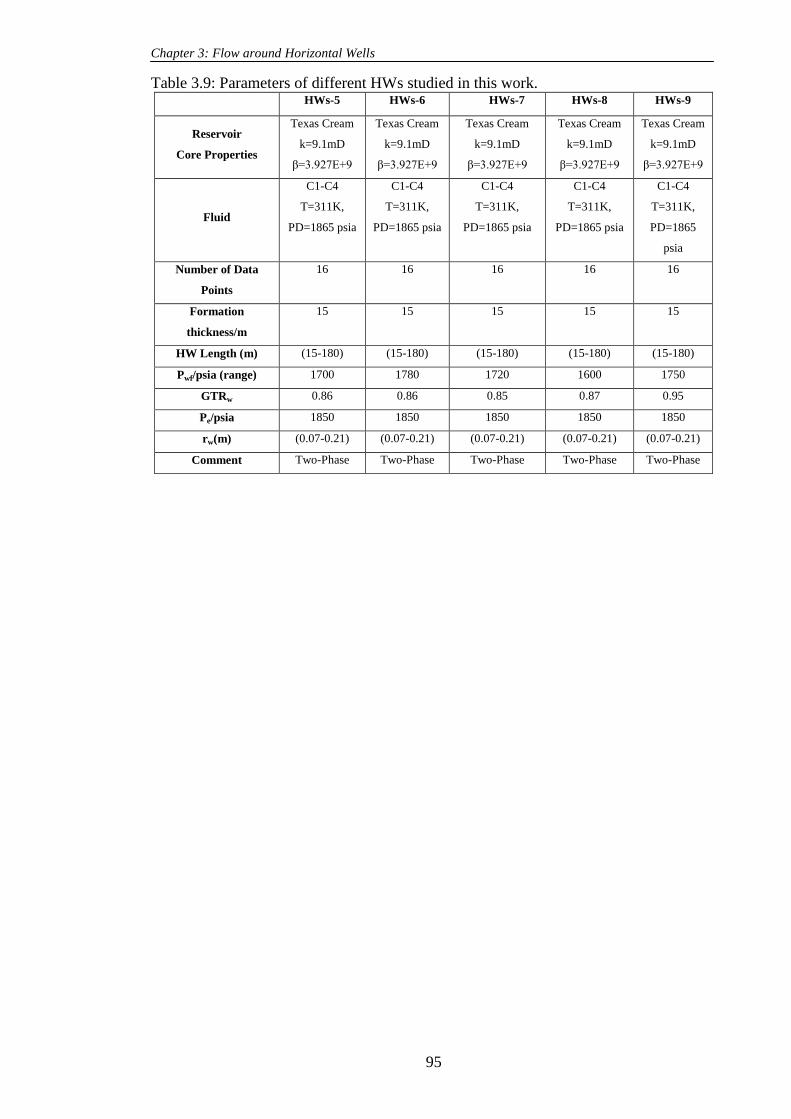
Chapter 3: Flow around Horizontal Wells
95
Table 3.9: Parameters of different HWs studied in this work. HWs-5 HWs-6 HWs-7 HWs-8 HWs-9
Reservoir
Core Properties
Texas Cream
k=9.1mD
β=3.927E+9
Texas Cream
k=9.1mD
β=3.927E+9
Texas Cream
k=9.1mD
β=3.927E+9
Texas Cream
k=9.1mD
β=3.927E+9
Texas Cream
k=9.1mD
β=3.927E+9
Fluid
C1-C4
T=311K,
PD=1865 psia
C1-C4
T=311K,
PD=1865 psia
C1-C4
T=311K,
PD=1865 psia
C1-C4
T=311K,
PD=1865 psia
C1-C4
T=311K,
PD=1865
psia
Number of Data
Points
16 16 16 16 16
Formation
thickness/m
15 15 15 15 15
HW Length (m) (15-180) (15-180) (15-180) (15-180) (15-180)
Pwf/psia (range) 1700 1780 1720 1600 1750
GTRw 0.86 0.86 0.85 0.87 0.95
Pe/psia 1850 1850 1850 1850 1850
rw(m) (0.07-0.21) (0.07-0.21) (0.07-0.21) (0.07-0.21) (0.07-0.21)
Comment Two-Phase Two-Phase Two-Phase Two-Phase Two-Phase
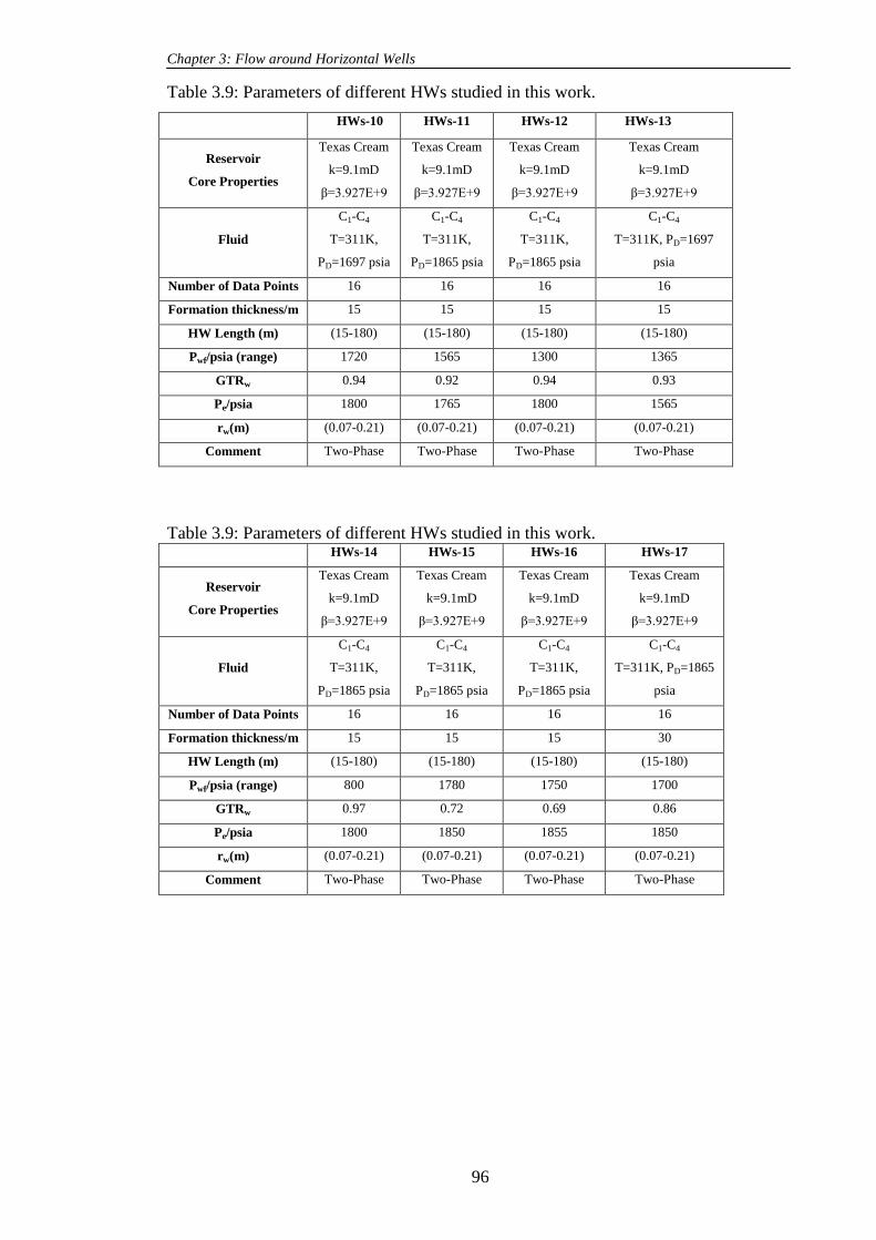
Chapter 3: Flow around Horizontal Wells
96
Table 3.9: Parameters of different HWs studied in this work.
HWs-10 HWs-11 HWs-12 HWs-13
Reservoir
Core Properties
Texas Cream
k=9.1mD
β=3.927E+9
Texas Cream
k=9.1mD
β=3.927E+9
Texas Cream
k=9.1mD
β=3.927E+9
Texas Cream
k=9.1mD
β=3.927E+9
Fluid
C1-C4
T=311K,
PD=1697 psia
C1-C4
T=311K,
PD=1865 psia
C1-C4
T=311K,
PD=1865 psia
C1-C4
T=311K, PD=1697
psia
Number of Data Points 16 16 16 16
Formation thickness/m 15 15 15 15
HW Length (m) (15-180) (15-180) (15-180) (15-180)
Pwf/psia (range) 1720 1565 1300 1365
GTRw 0.94 0.92 0.94 0.93
Pe/psia 1800 1765 1800 1565
rw(m) (0.07-0.21) (0.07-0.21) (0.07-0.21) (0.07-0.21)
Comment Two-Phase Two-Phase Two-Phase Two-Phase
Table 3.9: Parameters of different HWs studied in this work. HWs-14 HWs-15 HWs-16 HWs-17
Reservoir
Core Properties
Texas Cream
k=9.1mD
β=3.927E+9
Texas Cream
k=9.1mD
β=3.927E+9
Texas Cream
k=9.1mD
β=3.927E+9
Texas Cream
k=9.1mD
β=3.927E+9
Fluid
C1-C4
T=311K,
PD=1865 psia
C1-C4
T=311K,
PD=1865 psia
C1-C4
T=311K,
PD=1865 psia
C1-C4
T=311K, PD=1865
psia
Number of Data Points 16 16 16 16
Formation thickness/m 15 15 15 30
HW Length (m) (15-180) (15-180) (15-180) (15-180)
Pwf/psia (range) 800 1780 1750 1700
GTRw 0.97 0.72 0.69 0.86
Pe/psia 1800 1850 1855 1850
rw(m) (0.07-0.21) (0.07-0.21) (0.07-0.21) (0.07-0.21)
Comment Two-Phase Two-Phase Two-Phase Two-Phase

Chapter 3: Flow around Horizontal Wells
97
Table 3.9: Parameters of different HWs studied in this work.
HWs-14 HWs-15 HWs-16 HWs-17
Reservoir
Core Properties
Texas Cream
k=9.1mD
β=3.927E+9
Texas Cream
k=9.1mD
β=3.927E+9
Texas Cream
k=9.1mD
β=3.927E+9
Texas Cream
k=9.1mD
β=3.927E+9
Fluid
C1-C4
T=311K,
PD=1865 psia
C1-C4
T=311K,
PD=1697 psia
C1-C4
T=311K,
PD=1865 psia
C1-C4
T=311K,
PD=1865 psia
Number of Data Points 16 16 16 16
Formation thickness/m 30 30 30 30
HW Length (m) (15-180) (15-180) (15-180) (15-180)
Pwf/psia (range) 1780 1720 1600 1750
GTRw 0.86 0.85 0.87 0.95
Pe/psia 1850 1850 1850 1850
rw(m) (0.07-0.21) (0.07-0.21) (0.07-0.21) (0.07-0.21)
Comment Two-Phase Two-Phase Two-Phase Two-Phase
Table 3.9: Parameters of different HWs studied in this work. HWs-18 HWs-19 HWs-20 HWs-21
Reservoir
Core Properties
Texas Cream
k=9.1mD
β=3.927E+9
Texas Cream
k=9.1mD
β=3.927E+9
Texas Cream
k=9.1mD
β=3.927E+9
Texas Cream
k=9.1mD
β=3.927E+9
Fluid
C1-C4
T=311K,
PD=1697 psia
C1-C4
T=311K,
PD=1865 psia
C1-C4
T=311K,
PD=1865 psia
C1-C4
T=311K,
PD=1697 psia
Number of Data Points 16 16 16 16
Formation thickness/m 30 30 30 30
HW Length (m) (15-180) (15-180) (15-180) (15-180)
Pwf/psia (range) 1720 1565 1300 1365
GTRw 0.94 0.92 0.94 0.93
Pe/psia 1800 1765 1800 1565
rw(m) (0.07-0.21) (0.07-0.21) (0.07-0.21) (0.07-0.21)
Comment Two-Phase Two-Phase Two-Phase Two-Phase

Chapter 3: Flow around Horizontal Wells
98
Table 3.9: Parameters of different HWs studied in this work.
HWs-22 HWs-23 HWs-24 HWs-25 HWs-26
Reservoir
Core Properties
Texas Cream
k=9.1mD
β=3.927E+9
Texas Cream
k=9.1mD
β=3.927E+9
Texas Cream
k=9.1mD
β=3.927E+9
Texas Cream
k=9.1mD
β=3.927E+9
Texas Cream
k=9.1mD
β=3.927E+9
Fluid
C1-C4
T=311K,
PD=1865 psia
C1-C4
T=311K,
PD=1865 psia
C1-C4
T=311K,
PD=1697 psia
C1-C4
T=311K,
PD=1865 psia
C1-C4
T=311K,
PD=1865 psia
Number of Data
Points
16 16 16 16 16
Formation
thickness/m
30 45 45 45 45
HW Length (m) (15-180) (15-180) (15-180) (15-180) (15-180)
Pwf/psia (range) 800 800 1365 1700 1780
GTRw 0.97 0.97 0.93 0.86 0.86
Pe/psia 1800 1800 1565 1850 1850
rw(m) (0.07-0.21) (0.07-0.21) (0.07-0.21) (0.07-0.21) (0.07-0.21)
Comment Two-Phase Two-Phase Two-Phase Two-Phase Two-Phase
Table 3.9: Parameters of different HWs studied in this work. HWs-27 HWs-28 HWs-29 HWs-30
Reservoir
Core Properties
Texas Cream
k=9.1mD
β=3.927E+9
Texas Cream
k=9.1mD
β=3.927E+9
Texas Cream
k=9.1mD
β=3.927E+9
Texas Cream
k=9.1mD
β=3.927E+9
Fluid
C1-C4
T=311K,
PD=1697 psia
C1-C4
T=311K,
PD=1865 psia
C1-C4
T=311K,
PD=1865 psia
C1-C4
T=311K,
PD=1697 psia
Number of Data Points 16 16 16 16
Formation thickness/m 45 45 45 45
HW Length (m) (15-180) (15-180) (15-180) (15-180)
Pwf/psia (range) 1720 1600 1750 1720
GTRw 0.85 0.87 0.95 0.94
Pe/psia 1850 1850 1850 1800
rw(m) (0.07-0.21) (0.07-0.21) (0.07-0.21) (0.07-0.21)
Comment Two-Phase Two-Phase Two-Phase Two-Phase

Chapter 3: Flow around Horizontal Wells
99
Table 3.9: Parameters of different HWs studied in this work.
HWs-31 HWs-32 HWs-33 HWs-34
Reservoir
Core Properties
Texas Cream
k=9.1mD
β=3.927E+9
Texas Cream
k=9.1mD
β=3.927E+9
Texas Cream
k=9.1mD
β=3.927E+9
Texas Cream
k=9.1mD
β=3.927E+9
Fluid
C1-C4
T=311K,
PD=1865 psia
C1-C4
T=311K,
PD=1865 psia
C1-C4
T=311K,
PD=1697 psia
C1-C4
T=311K,
PD=1865 psia
Number of Data Points 16 16 16 16
Formation thickness/m 45 45 45 45
HW Length (m) (15-180) (15-180) (15-180) (15-180)
Pwf/psia (range) 1565 1300 1365 800
GTRw 0.92 0.94 0.93 0.97
Pe/psia 1765 1800 1565 1800
rw(m) (0.07-0.21) (0.07-0.21) (0.07-0.21) (0.07-0.21)
Comment Two-Phase Two-Phase Two-Phase Two-Phase
Table 3.9: Parameters of different HWs studied in this work. HWs-35 HWs-36
Reservoir
Core Properties
Texas Cream
k=9.1mD
β=3.927E+9
Texas Cream
k=9.1mD
β=3.927E+9
Fluid
C1-C4
T=311K,
PD=1865 psia
C1-C4
T=311K,
PD=1865 psia
Number of Data Points 1 1
Formation thickness/m 15 15
HW Length (m) 15 15
Pwf/psia (range) 1565 1365
GTRw 0.87 0.9
Pe/psia --- ---
rw(m) 0.07 0.07
Comment Two-Phase Two-Phase

Chapter 3: Flow around Horizontal Wells
100
Table 3.10: The initial reservoir conditions and mass flow rates for Two-Phase PSS
HWs models studied here.
HWs Model Pres (psi) Qt(m3/day) GTRwell
A 1557 31.36 0.79
B 1493 35 0.89
Table 3.11: The well geometries and initial reservoir conditions for two-phase PSS
HWs models studied here. HWs-PSS1 HWs-PSS2
Reservoir
Core Properties
Texas Cream
k=9.1mD
β=3.927E+9
Texas Cream
k=9.1mD
β=3.927E+9
Fluid
C1-C4
T=311K,
PD=1865 psia
C1-C4
T=311K,
PD=1865 psia
Number of Data Points 1 1
Formation thickness/m 15 15
HW Length (m) 15 15
Pwf/psia (range) 1565 1365
GTRw 0.87 0.9
Pe/psia --- ---
rw(m) 0.07 0.07
Comment Two-Phase Two-Phase

Chapter 3: Flow around Horizontal Wells
101
(a)
(b)
Figure 3.1: a) An ellipsoid drainage volume; b) Dividing 3-D problems into two 2D
problems (vertical and horizontal planes), Joshi (1988).
Horizontal Well
B
B
A A
B
B

Chapter 3: Flow around Horizontal Wells
102
Figure 3.2: The HW drainage area, a rectangular with two semi circles at the ends, used
for semi analytical solutions by Giger (1985) and Renarld and Dupuy (1991).

Chapter 3: Flow around Horizontal Wells
103
(a)
(b)
Figure 3.3: (a) Gas production rate and (b) Total gas production versus time for the
horizontal wells with length of 1550, 1150, 750, and 350 ft, and a vertical well, all in
the reservoir with 50 ft thickness, Model A of Table 3.1.
Length=1550
ft
Length=1150
ft
Length=750
ft
Length=350
ft
Vertical well
Length=1550
ft
Length=1150 ft
Length=750
ft
Length=350
ft
Vertical well

Chapter 3: Flow around Horizontal Wells
104
0.00
5.00
10.00
15.00
20.00
25.00
30.00
35.00
0 1000 2000 3000 4000 5000 6000 7000
Time (DAYS)
D(F
GP
T)v
-h%
Difference 200 ftDifference 100ftDifference 50 ft
(a)
0.00
10.00
20.00
30.00
40.00
50.00
60.00
70.00
80.00
90.00
100.00
0 1000 2000 3000 4000 5000 6000 7000
Time (DAYS)
D(F
GP
T)v
-h%
Difference 200 ftDifference 100ftDifference 50 ft
(b)
Figure 3.4: Relative increase in cumulative gas production in horizontal wells
compared to that of the vertical well Pw<Pdew : a) horizontal well length= 350; ft b)
horizontal well length= 1550 ft, Model A of Table 3.2.

Chapter 3: Flow around Horizontal Wells
105
Figure 3.5: Total gas production vs. time, with and without considering coupling and
inertial effects, Model B (Table 3. 2), Texas Cream core properties, Lhw=100 ft.
Figure 3.6: Total gas production vs. time, with and without considering coupling and
inertial effects, Model B (Table 3.2), Lhw=300 ft, Texas Cream core properties.
Inertial & Coupling - on
Inertial & Coupling-off
Inertial-on
Inertial & Coupling - on
Inertial & Coupling-off
Inertial-on

Chapter 3: Flow around Horizontal Wells
106
Figure 3.7: Total gas production vs. time, with and without considering coupling and
inertial effects, Model B (Table 3.2), Lhw=700 ft, Texas Cream core properties.
Figure 3.8: Total gas production vs. time, with and without considering coupling and
inertial effects, Model B (Table 3.2), Lhw=900 ft, Texas Cream core properties.
Inertial & Coupling - on
Inertial & Coupling-off
Inertial-on
Inertial & Coupling - on
Inertial & Coupling-off
Inertial-on

Chapter 3: Flow around Horizontal Wells
107
Figure 3.9: Total gas production vs. time, with and without considering coupling and
inertial effects, Model B (Table 3.2), Lhw=200 ft, Berea core properties.
Figure 3.10: Total gas production vs. time, with and without considering coupling and
inertial effects, Model B (Table 3.2), Lhw=500 ft, Berea core properties.
Inertial & Coupling - on
Inertial & Coupling-off
Inertial-on
Inertial & Coupling - on
Inertial & Coupling-off
Inertial-on

Chapter 3: Flow around Horizontal Wells
108
Figure 3.11: Total gas production vs. time, with and without considering coupling and
inertial effects, Model B (Table 3.2), Lhw=100 ft, RC1b core properties.
Figure 3.12: Total gas production vs. time, with and without considering coupling and
inertial effects, Model B (Table 3.2), Lhw=200 ft, RC1b core properties.
Inertial & Coupling - on
Inertial & Coupling-off
Inertial-on
Inertial & Coupling - on
Inertial & Coupling-off
Inertial-on

Chapter 3: Flow around Horizontal Wells
109
Figure 3.13: The total gas production vs. time, , with and without considering coupling
and inertial effects, Model B (Table 3.2) ,Lhw=500 ft, RC1b core properties.
Figure 3.14: The total gas production vs. time, with and without considering coupling
and inertial effects, Model B (Table 3.2), Lhw=900 ft, RC1b core properties.
Inertial & Coupling - on
Inertial & Coupling-off
Inertial-on
Inertial & Coupling - on
Inertial & Coupling-off
Inertial-on

Chapter 3: Flow around Horizontal Wells
110
Figure 3.15: 3-D Geometry of the horizontal well in this study.
Figure 3.16: Triangular mesh element showing the longest side, shortest side, maximum
interior angle and the minimum interior angle, (Mesh quality tutorials (rocksceince)).
Maximum interior angle
Minimum interior angle
Shortest side

Chapter 3: Flow around Horizontal Wells
111
(a)
(b)
Figure 3.17: a) En example of the defined mesh the reservoir model (object) for one of
the cases studied here b) the refined and specified elements around the horizontal well.

Chapter 3: Flow around Horizontal Wells
112
Figure 3.18: The mesh quality of the reservoir model of Figure 3.17.
Figure 3.19: The pressure distribution around the HW for the selected model shown in
Tables 3.17 and 3.18.

Chapter 3: Flow around Horizontal Wells
113
0
0.5
1
1.5
2
2.5
3
3.5
4
4.5
5
0 1 2 3 4 5
Mass Flow Rate (kg/s)-ECLIPSE
Mas
s F
low
Rat
e (k
g/s
)- i
n-h
ou
se S
imu
lato
r
Figure 3.20: Comparison between the mass flow rates estimated using the in-house and
ECLIPSE simulators.

Chapter 3: Flow around Horizontal Wells
114
1
1.5
2
2.5
3
3.5
4
4.5
5
5.5
6
0 0.2 0.4 0.6 0.8 1
kv/kh
PR
(HW
/VW
)
Normal (10500) grid
Fine grid (21000) grid
Extremely fine (168000) grid
Comsol-Isotropic Mesh
Comsol-Anistropic Mesh
(a)
0
0.5
1
1.5
2
2.5
3
3.5
4
0 0.02 0.04 0.06 0.08 0.1
kv/kh
PR
(HW
/VW
)
Comsol-Isotropic Mesh
Comsol-Anistropic Mesh
(b)
Figure 3.21: The productivity ratio (horizontal well to vertical well) versus the
permeability anisotropy index.

Chapter 3: Flow around Horizontal Wells
115
kv/kh=1.0-AD% S-Joshi 's Eq. with in-house-values
0
50
100
150
200
250
1 6 11 16 21
L/h
AD
%-J
osh
i 's
Eq
. w
ith
S-o
utc
om
e
sim
ula
tor
AD% Joshi 's Eq.
(a)
kv/kh=1.0-AD% S-Borosiv 's Eq. with S-outcome of simulator
0
5
10
15
20
25
30
35
1 6 11 16 21L/h
AD
%-B
oro
siv
e 's
Eq
. w
ith
S-
ou
tco
me
sim
ula
tor
AD% Borosiv 's Eq.
(b)
Figure 3.22: Absolute deviation error skin values calculated using a) Joshi„s and b)
Borosiv„s equation and those obtained by applying the calculated in-house simulator
mass flow rates into Equation 3.8.

Chapter 3: Flow around Horizontal Wells
116
-6.5
-4.5
-2.5
-0.5
1.5
3.5
1 6 11 16 21L/h
Sm
Joshi's Eq.
Joshi-Economides 's Eq
Outcome in house simulator
(a)
-6.5
-4.5
-2.5
-0.5
1.5
3.5
1 6 11 16 21L/h
Sm
Joshi's Eq.
Joshi-Economides 's Eq
Outcome in house simulator
(b)
Figure 3.23: Comparison of the calculated skin using Joshi‟s and Joshi-Economides„s
equations with those obtained by applying the calculated in-house simulator mass flow
rates into Equation 3.8, anisotropic reservoir, kvkh= [0.6 0.4].
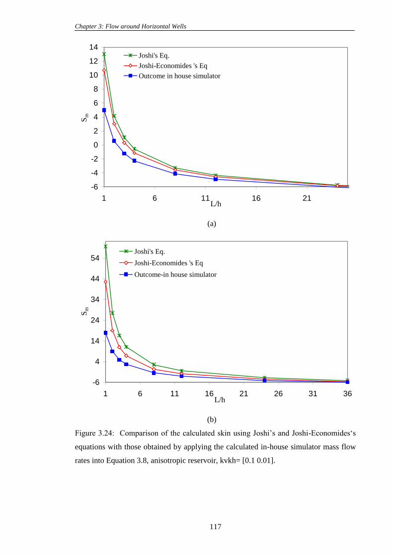
Chapter 3: Flow around Horizontal Wells
117
-6
-4
-2
0
2
4
6
8
10
12
14
1 6 11 16 21L/h
Sm
Joshi's Eq.
Joshi-Economides 's Eq
Outcome in house simulator
(a)
-6
4
14
24
34
44
54
1 6 11 16 21 26 31 36L/h
Sm
Joshi's Eq.
Joshi-Economides 's Eq
Outcome-in house simulator
(b)
Figure 3.24: Comparison of the calculated skin using Joshi‟s and Joshi-Economides„s
equations with those obtained by applying the calculated in-house simulator mass flow
rates into Equation 3.8, anisotropic reservoir, kvkh= [0.1 0.01].

Chapter 3: Flow around Horizontal Wells
118
(a)
(b)
Figure 3.25: a) A schematic image of thin layer model; b) The pressure profile across
the reservoir for the extreme anisotropic case of kv=0.

Chapter 3: Flow around Horizontal Wells
119
Figure 3.26: The schematic flow diagram of a fully penetrating HW in an isotropic
reservoir.
h

Chapter 3: Flow around Horizontal Wells
120
0
10
20
30
40
50
60
70
80
0 10 20 30 40 50 60 70 80
Sm-In house simulator values
Sm
-Pre
dic
ted
by
Co
rrel
atio
n
-9
-8
-7
-6
-5
-4
-3
-2
-1
0
-9 -8 -7 -6 -5 -4 -3 -2 -1 0
Sm-In house simulator values
Sm
-Pre
dic
ted
by
Co
rrel
atio
n
Figure 3.27: Comparison of geometric skin values calculated using the proposed Sm
correlation with those obtained by applying the calculated HW in-house simulator mass
flow rates into Equation 3.8.

Chapter 3: Flow around Horizontal Wells
121
-9
-8
-7
-6
-5
-4
-3
-2
-1
0
-9 -8 -7 -6 -5 -4 -3 -2 -1 0
Sm-In house simulator values
Sm
-Pre
dic
ted
by
Co
rrel
atio
n
Figure 3.28: Comparison of the geometric skin values calculated using the author‟s
proposed correlation and the corresponding values from the in-house simulator, new
data points not used in the development of the correlation.
-8
-7
-6
-5
-4
-3
-2
-1
0
-8 -7 -6 -5 -4 -3 -2 -1 0
Mechanical Skin- Joshi & Borosive
Mec
han
ical
Sk
in-C
orr
elat
ion
Borosive-Equation
Joshi-Equation
Figure 3.29: Comparison between geometric skin values calculated using the author„s
proposed correlation and the corresponding values using Joshi‟s (1991) and Borosiv‟s
(1984) semi-analytical equations.

Chapter 3: Flow around Horizontal Wells
122
0
1
2
3
4
5
6
0 200 400 600 800 1000 1200 1400 1600
Horizontal well lenght(m)
PR
(H
W/V
W)
h=15 m
h=30 m
h=45 m
Figure 3.30: Productivity ratios of a HW to a VW versus HW length, effect of reservoir
thickness.
0
1
2
3
4
5
6
7
0 200 400 600 800 1000 1200 1400 1600
Horizontal well length (m)
PR
(H
W/V
W)
Rw=0.07 m
Rw=0.14 m
Rw=0.21 m
Figure 3.31: Productivity ratio of a HW to a VW versus length, effect of wellbore
radius.

Chapter 3: Flow around Horizontal Wells
123
0
1
2
3
4
5
6
7
0 200 400 600 800 1000 1200 1400 1600
Horizontal well length(m)
PR
(H
W/V
W)
kvkh=1.0
kvkh=0.1
kvkh=0.01
kvkh=0.001
Figure 3.32: Productivity ratio of a HW to a VW versus length, effect of anisotropy.
Figure 3.33: Flow pattern and pressure distribution of a fully horizontal well.
Heal
Toe

Chapter 3: Flow around Horizontal Wells
124
Figure 3.34: Flow pattern and pressure distribution of a partially horizontal well.
0
0.1
0.2
0.3
0.4
0.5
0.6
0.7
0.8
0.9
1
0 0.2 0.4 0.6 0.8 1
L/Xres
(PR
)pp
/(P
R)f
p
L=60 m
L=180 m
L=720 m
Figure 3.35: Productivity ratio of partially to fully penetrating horizontal wells versus
penetration ratio at three different horizontal well lengths, rw=0.14 m, h=30 m.
Heal
Toe

Chapter 3: Flow around Horizontal Wells
125
-7.5
-6
-4.5
-3
-1.5
0
0 0.2 0.4 0.6 0.8 1L/Xres
Mec
han
ical
sk
in
L=60 m
L=180 m
L=720 m
Figure 3.36: Variation of geometric skin with partial penetration ratio at three different
horizontal well lengths, h=30 m and rw=0.14 m.
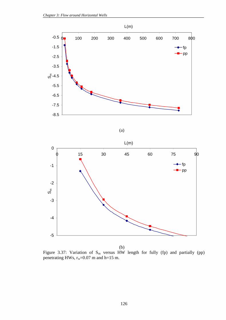
Chapter 3: Flow around Horizontal Wells
126
-8.5
-7.5
-6.5
-5.5
-4.5
-3.5
-2.5
-1.5
-0.5 0 100 200 300 400 500 600 700 800
L(m)
Sm
fp
pp
(a)
-5
-4
-3
-2
-1
0
0 15 30 45 60 75 90
L(m)
Sm
fp
pp
(b)
Figure 3.37: Variation of Sm versus HW length for fully (fp) and partially (pp)
penetrating HWs, rw=0.07 m and h=15 m.

Chapter 3: Flow around Horizontal Wells
127
0
0.05
0.1
0.15
0.2
0.25
0 10 20 30 40 50 60 70 80 90
L/h
Rel
ativ
e in
crea
se i
n M
ech
anic
al S
kin
(S
pp
)/S
mp
p h= 15 m
h= 30 m
Figure 3.38: Variation of relative increase in geometric skin versus length to thickness
ratio, rw=0.14 m.

Chapter 3: Flow around Horizontal Wells
128
-9
-8
-7
-6
-5
-4
-3
-2
-1
0
-9 -8 -7 -6 -5 -4 -3 -2 -1 0
Predicted Sm considering pp effect using the correlation
Cal
cula
ted
Sm
usi
ng
th
e in
-ho
use
sim
ula
tor
(a)
-9
-8
-7
-6
-5
-4
-3
-2
-1
0
-9 -8 -7 -6 -5 -4 -3 -2 -1 0
Predicted Sm considering pp effect using the correlation
Cal
cula
ted
Sm
usi
ng
th
e in
-ho
use
sim
ula
tor
(b)
Figure 3.39: The predicted Sm, including partial penetration effect using the author„s
proposed correlation (Equation 3.40 and 3.41), versus the corresponding values
obtained using the in-house simulator, a) 1resX
L b) 8.0
resX
L.

Chapter 3: Flow around Horizontal Wells
129
-9
-8
-7
-6
-5
-4
-3
-2
-1
0
0 200 400 600 800 1000 1200 1400 1600
Lhw(m)
Sm
Central Location
Z=h/6
Z=3h/10
Z=3h/4
(a)
-5
-4.5
-4
-3.5
-3
-2.5
-2
-1.5
-1
-0.5
0
0 50 100 150 200
Lhw(m)
Sm
Central Location
Z=h/6
Z=3h/10
Z=3h/4
(b)
Figure 3.40: Variation of geometric skin versus the HW length for a HW located a
distance from the formation centre, h/2, in the z direction.

Chapter 3: Flow around Horizontal Wells
130
-8
-7
-6
-5
-4
-3
-2
-1
0
-8 -7 -6 -5 -4 -3 -2 -1 0
St- Correlation
St-
In-h
ou
se s
imula
tor
Figure 3.41: Comparing zmt SSS calculated by the author„s proposed correlation,
Equation 3.45, against those obtained by the HW in-house simulator.
0
10
20
30
40
50
60
70
80
0 10 20 30 40 50 60 70 80
Mass Flow Rate(kg/s)-In house simulator
Mas
s F
low
Rat
e(k
g/s
)-E
OH
Figure 3.42: Comparison of mass flow rate of a HW calculated using in-house simulator
with predicted mass flow rate by the equivalent open hole (EOH) model, using the
effective wellbore radius, HW-1 data set of Table 3.6.
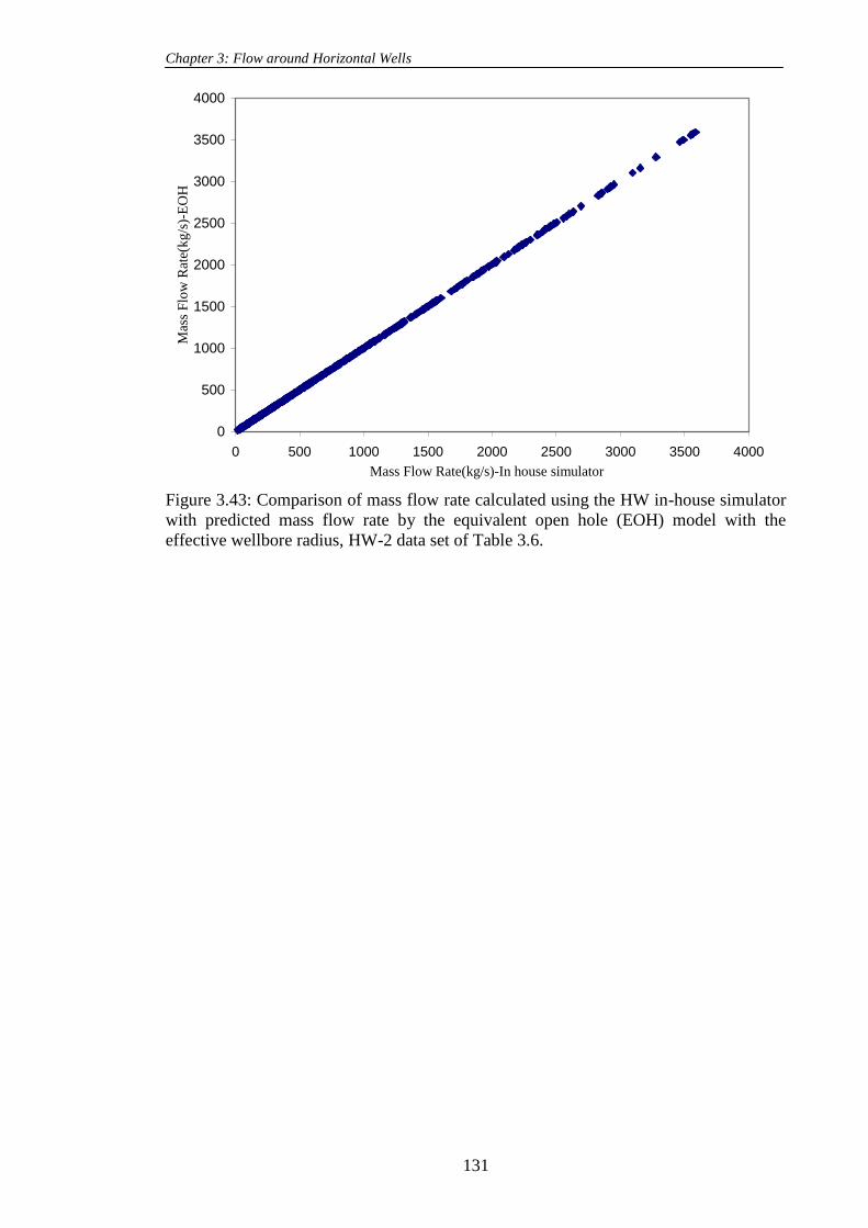
Chapter 3: Flow around Horizontal Wells
131
0
500
1000
1500
2000
2500
3000
3500
4000
0 500 1000 1500 2000 2500 3000 3500 4000
Mass Flow Rate(kg/s)-In house simulator
Mas
s F
low
Rat
e(k
g/s
)-E
OH
Figure 3.43: Comparison of mass flow rate calculated using the HW in-house simulator
with predicted mass flow rate by the equivalent open hole (EOH) model with the
effective wellbore radius, HW-2 data set of Table 3.6.

Chapter 3: Flow around Horizontal Wells
132
(a)
(b)
3.44: Isobar curves around a horizontal well a) without and b) with inertia (non-
Darcy).

Chapter 3: Flow around Horizontal Wells
133
Figure 3.45: rk distribution for non-Darcy flow around a horizontal well.
0
0.1
0.2
0.3
0.4
0.5
0.6
0.7
0.8
0.9
0 200 400 600 800 1000 1200 1400 1600
Horizontal well length(m)
Sf
h= 15 m
h= 30 m
h= 45 m
Figure 3.46: Variation of the flow skin Sf versus horizontal well length at three different
reservoir thicknesses, HW-2 data set of Table 3.6, rw= 0.14 m.

Chapter 3: Flow around Horizontal Wells
134
0
0.2
0.4
0.6
0.8
1
1.2
1.4
1.6
0 100 200 300 400 500 600
Horizontal well lenght(m)
Sf
rw= 0.07 m
rw= 0.14 m
rw= 0.21 m
Figure 3.47: Variation of the flow skin Sf versus horizontal well length at three different
wellbore radii, HW-2 data set of Table 3.6, h= 15 m.
0
0.2
0.4
0.6
0.8
1
1.2
1.4
0 500 1000 1500 2000 2500
Velocity at the HW surface (m/day)
Sf
L/h=2
L/h=4
L/h=8
L/h=12
Figure 3.48: Variation of the flow skin (Sf) versus velocity at different HW lengths to
the reservoir thickness, HW-1 data set of Table 3.6, h=45 m.

Chapter 3: Flow around Horizontal Wells
135
0
0.2
0.4
0.6
0.8
1
1.2
1.4
1.6
0 1000 2000 3000 4000 5000 6000 7000 8000 9000
Velocity at the HW surfaces (m/days)
Sf
L/h=2
L/h=4
L/h=12
L/h=16
L/h=20
Figure 3.49: Variation of the flow skin Sf versus velocity at different HW lengths to the
reservoir thickness, HW-2 data set of Table 3.6, h=45 m.

Chapter 3: Flow around Horizontal Wells
136
3
3.5
4
4.5
5
5.5
6
6.5
7
0 2000 4000 6000 8000 10000 12000
Velocity at the HW Surface (m/day)
PR
(H
W/
VW
)
L= 90 m
L= 120 m
L= 180 m
L= 360 m
(a)
3
3.5
4
4.5
5
5.5
0 100 200 300 400 500 600 700 800 900
Velocity at the HW Surface (m/day)
PR
(H
W/
VW
)
L= 90 m
L= 120 m
L= 180 m
L= 360 m
(b)
Figure 3.50: Productivity ratio (horizontal to vertical well) versus velocity at four
different HW lengths, rw=0.14 m, h=15 m , Pw=1000 psi a) Berea b)Texas Cream core
properties .

Chapter 3: Flow around Horizontal Wells
137
0
1
2
3
4
5
6
7
8
0 200 400 600 800 1000 1200 1400 1600
L (m)
PR
(H
W/
VW
)
Non-Darcy flow
Darcy flow
(a)
0
1
2
3
4
5
6
7
0 200 400 600 800 1000 1200 1400 1600
L (m)
PR
(H
W/
VW
)
Non-Darcy flow
Darcy flow
(b)
Figure 3.51: Productivity ratio (horizontal to vertical well) versus horizontal well length
for Darcy and non Darcy flow regimes, rw=0.14 m, h=15 m, Pw=1000 psi and Pres= 6200
psi a) Berea b)Texas Cream core properties.

Chapter 3: Flow around Horizontal Wells
138
3.00
3.20
3.40
3.60
3.80
4.00
4.20
4.40
0 2000 4000 6000 8000 10000 12000
Velocity at the HW Surface (m/day)
PR
(H
W/
VW
)
rw=0.07 m
rw=0.14 m
rw=0.21 m
(a)
3.10
3.20
3.30
3.40
3.50
3.60
3.70
0 200 400 600 800 1000 1200 1400 1600
Velocity at the HW Surface (m/day)
PR
(H
W/
VW
)
rw=0.07 m
rw=0.14 m
rw=0.21 m
(b)
Figure 3.52: Productivity ratio (horizontal to vertical well) versus velocity for three
wellbore radii, L=90 m, h=15 m, Pw=1000 psi, a) Berea b) Texas Cream core properties.

Chapter 3: Flow around Horizontal Wells
139
3.00
3.10
3.20
3.30
3.40
3.50
3.60
3.70
3.80
0 200 400 600 800 1000
Velocity at the HW Surface (m/day)
PR
(H
W/
VW
)
Berea
Texas Cream
Figure 3.53: Productivity ratio (horizontal to vertical well) versus velocity, L=90 m,
h=15 m, Pw=1000 psi, rw=0.14 m for Berea and Texas Cream core properties.
0.6
0.65
0.7
0.75
0.8
0.85
0.9
0.95
1
0 500 1000 1500 2000 2500
Velocity at the HW Surface (m/day)
(PI)
No
n D
arcy
/(P
I)D
arcy
L=30 m
L=90 m
L=180 m
Figure 3.54: Productivity ratio (Non Darcy to Darcy flow) versus velocity for the
different HW lengths, h=15 m, Pw=1000 psi, rw=0.14 m for Texas Cream core
properties.

Chapter 3: Flow around Horizontal Wells
140
0
200
400
600
800
1000
1200
1400
0 200 400 600 800 1000 1200 1400Mass Flow Rate(kg/s)
In-house simulator
Mas
s F
low
Rat
e(k
g/s
)
EO
H
Figure 3.55: The mass flow rate calculated using the author„s proposed effective
equivalent wellbore radius correlation based on the equivalent radius concept versus the
corresponding values obtained by the in-house simulator, Berea core properties.
0
20
40
60
80
100
120
140
160
180
200
0 20 40 60 80 100 120 140 160 180 200Mass Flow Rate(kg/s)
In-house Simulator (HW)
Mas
s F
low
Rat
e(kg/s
)
EO
H
Figure 3.56: The mass flow rate calculated using the author„s proposed effective
equivalent wellbore radius correlation based on the equivalent radius concept versus the
corresponding values obtained by the in-house simulator, Texas Cream core properties.

Chapter 3: Flow around Horizontal Wells
141
0
0.02
0.04
0.06
0.08
0.1
0.12
0 0.02 0.04 0.06 0.08 0.1 0.12ECLIPSE (kg/s)
CO
MS
OL
(k
g/s
)
Figure 3.57: Comparison of the results of ECLIPSE two-phase model (gas and
condensate) with those of the in-house simulator at three different pressure drops and
fractional flow.

Chapter 3: Flow around Horizontal Wells
142
0
1
2
3
4
5
6
0 200 400 600 800 1000 1200 1400 1600
Horizontal Well Length (m)
PR
(H
W/V
W)
GTRw=0.941
GTRw=0.907
GTRw=0.809
(a)
0
0.5
1
1.5
2
2.5
3
3.5
4
4.5
0 100 200 300 400 500 600
Horizontal Well Length(m)
PR
(HW
/VW
)
GTRw=0.941
GTRw=0.907
GTRw=0.809
(b)
Figure 3.58: Productivity ratio (horizontal to vertical well) versus horizontal well length
at three different gas fractional flows, h= 15 m, Pres=1800 psi, Pw= 1300 psi, a) rw=0.14
m b) rw=0.21 m, Berea core properties.

Chapter 3: Flow around Horizontal Wells
143
0
0.5
1
1.5
2
2.5
3
3.5
4
4.5
0 100 200 300 400 500 600
Horizontal Well Length (m)
PR
(HW
/VW
)
rw=0.07 m
rw=0.14 m
rw=0.21 m
Figure 3.59: Productivity ratio versus horizontal well length at the wellbore radii of 0.07
m, 0.14 m and 0.21 m, GTR=0.809, h= 15 m, Pres=1800 psi, Pw= 1300 psi.
0
1
2
3
4
5
6
0 200 400 600 800 1000 1200 1400 1600
Horizontal Well Length (m)
PR
(HW
/VW
)
dp=200 psi-GTRw=0.81
dp=300 psi- GTRw=0.81
dp=400 psi- GTRw= 0.81
dp=200 psi- GTRw= 0.941
dp=300 psi- GTRw= 0.941
dp=400 psi- GTRw= 0.941
Figure 3.60: Productivity ratio versus horizontal well length, rw=0.14 m, GTRw=0.941
& 0.809, h= 15 m, Pw= 1300 psi, pressure drops of 200, 300 and 400 psi.

Chapter 3: Flow around Horizontal Wells
144
0
0.5
1
1.5
2
2.5
3
3.5
4
4.5
5
0 200 400 600 800 1000 1200 1400 1600
Horizontal well length(m)
PR
(H
W/V
W)
GTRw=0.941
GTRw=0.907
GTRw=0.809
(a)
0
0.5
1
1.5
2
2.5
3
3.5
4
4.5
0 100 200 300 400 500 600
Horizontal well length (m)
PR
(H
W/V
W)
GTRw=0.941
GTRw=0.907
GTRw=0.809
(b)
Figure 3.61: Productivity ratio versus horizontal well length at three different gas
fractional flows, h= 15 m, Pres=1800 psi, Pw= 1300 psi, a) rw=0.14 m b) rw=0.21 m,
Texas cream core properties.

Chapter 3: Flow around Horizontal Wells
145
(a)
(b)
Figure 3.62: a) Iso-pressure map b) Iso-condensate saturation map around a HW.
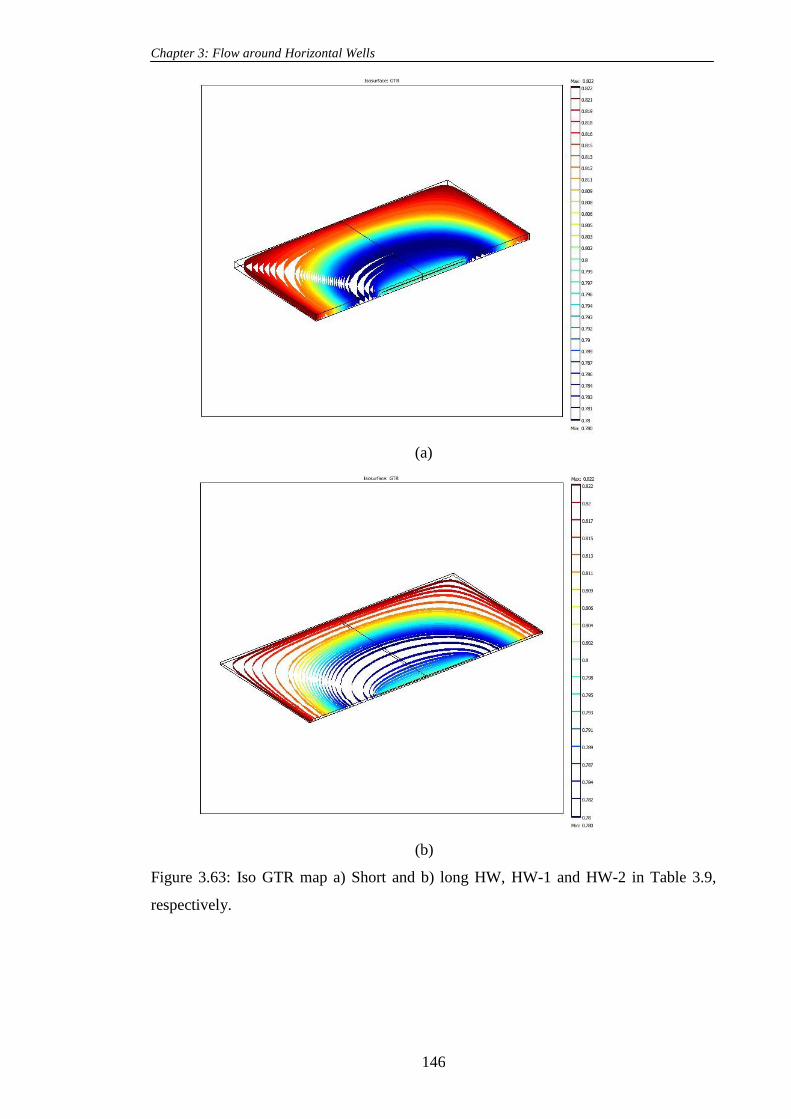
Chapter 3: Flow around Horizontal Wells
146
(a)
(b)
Figure 3.63: Iso GTR map a) Short and b) long HW, HW-1 and HW-2 in Table 3.9,
respectively.

Chapter 3: Flow around Horizontal Wells
147
(a)
(b)
Figure 3.64: Iso-pressure map a) Short and b) Long HW, HW-1 and HW2 in Table 3.9,
respectively.

Chapter 3: Flow around Horizontal Wells
148
0
0.1
0.2
0.3
0.4
0.5
0.6
0.7
0.8
0.9
0 10 20 30 40
R (m)
krg
1770
1780
1790
1800
1810
1820
1830
1840
1850
1860
krg
krgb
P (psi)
P (
psi
)
(a)
0
0.05
0.1
0.15
0.2
0.25
0.3
0 10 20 30 40
R(m)
krg
1710
1720
1730
1740
1750
1760
1770
1780
1790
1800
1810krg
krgb
P (psi) -IC
P(p
si)
(b)
Figure 3.65: Variation of affected (by coupling and inertia) gas relative permeability
and base relative permeability for EOH of a) HW-3 b) HW-4, listed in Table 3.9.
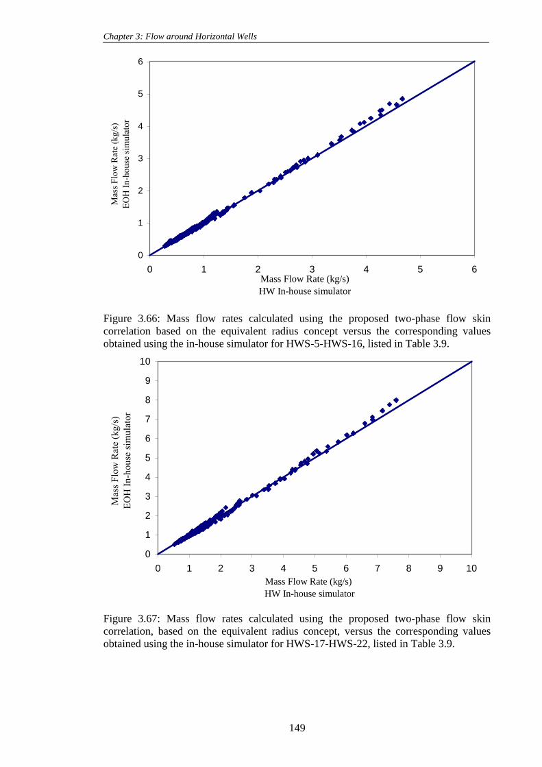
Chapter 3: Flow around Horizontal Wells
149
0
1
2
3
4
5
6
0 1 2 3 4 5 6Mass Flow Rate (kg/s)
HW In-house simulator
Mas
s F
low
Rat
e (k
g/s
)
EO
H I
n-h
ou
se s
imu
lato
r
Figure 3.66: Mass flow rates calculated using the proposed two-phase flow skin
correlation based on the equivalent radius concept versus the corresponding values
obtained using the in-house simulator for HWS-5-HWS-16, listed in Table 3.9.
0
1
2
3
4
5
6
7
8
9
10
0 1 2 3 4 5 6 7 8 9 10
Mass Flow Rate (kg/s)
HW In-house simulator
Mas
s F
low
Rat
e (k
g/s
)
EO
H I
n-h
ou
se s
imu
lato
r
Figure 3.67: Mass flow rates calculated using the proposed two-phase flow skin
correlation, based on the equivalent radius concept, versus the corresponding values
obtained using the in-house simulator for HWS-17-HWS-22, listed in Table 3.9.

Chapter 3: Flow around Horizontal Wells
150
0
1
2
3
4
5
6
7
8
9
0 1 2 3 4 5 6 7 8 9Mass Flow Rate (kg/s)
HW In-house simulator
Mas
s F
low
Rat
e (k
g/s
)
EO
H I
n-h
ou
se s
imu
lato
r
Figure 3.68: Mass flow rate calculated using the proposed two-phase flow skin
correlation, based on the equivalent radius concept, versus the corresponding values
obtained using the in-house simulator for HWS-23-HWS-34, listed in Table 3.9.
0
500
1000
1500
2000
2500
3000
3500
4000
0 500 1000 1500 2000 2500 3000 3500 4000
Pave (psi)-Eclipse HW model
Pav
e (p
si)-
In h
ou
se s
imu
lato
r H
W m
od
el (
Co
mso
l)
Figure 3.69: Comparison between the average pressures estimated using the in-house
simulator and ECLIPSE simulators, both operating under pseudo steady state
conditions, AAD% 1.

Chapter 3: Flow around Horizontal Wells
151
-9
-8
-7
-6
-5
-4
-3
-2
-1
0
0 200 400 600 800 1000 1200 1400
Horizontal Well Length(m)
Sm
SS
PSS
(a)
-8
-7
-6
-5
-4
-3
-2
-1
0
0 200 400 600 800 1000
Horizontal Well Length (m)
Sm
SS
PSS
(b)
Figure 3.70: Geometric skin calculated by the HW pseudo steady and steady state in-
house simulators versus HW length a) h=15 m b) h=30 m.

Chapter 3: Flow around Horizontal Wells
152
0
2
4
6
8
10
12
14
16
0 200 400 600 800 1000 1200 1400HW lenght (m)
AD
% e
rro
r
Figure 3.71: Variation of error on the pseudo-steady state horizontal well productivity
index (JD) obtained by ignoring the last two terms in the denominator of JD, Equation
3.102, versus HW lengths.
600
700
800
900
1000
1100
1200
1300
1400
1500
1600
0 20 40 60 80 100
Timestep
Pav
e(p
si)
Comsol
Eclipse
Figure 3.72: The calculated average pressure at the pseudo steady condition versus
timestep, obtained by the in-house simulator (Comsol) and the model constructed by
E300, Case A.

Chapter 3: Flow around Horizontal Wells
153
600
700
800
900
1000
1100
1200
1300
1400
1500
0 20 40 60 80 100
Timestep
Pav
e(p
si)
Comsol
Eclipse
Figure 3.73: The calculated average pressure at the pseudo steady condition versus
timestep obtained by the in-house simulator (Comsol) and the model constructed by
E300, Case B.
-0.6
-0.55
-0.5
-0.45
-0.4
-0.35
-0.3
-0.25
-0.2
1670 1680 1690 1700 1710 1720 1730 1740 1750
Pave (psi)
Sf
SS
PSS
Figure 3.74: Comparing the flow skins calculated using PSS and SS HW in house
simulators and EOH for HW1 Table3.11.

Chapter 4: Flow around Deviated Wells
154
FLOW AROUND DEVIATED WELLS
4.1 INTRODUCTION
In the last two decades, drilling horizontal (HWs) and deviated (DWs) wells has
become a common practice around the world. The major purpose of drilling such wells
is to achieve greater wellbore exposure to the reservoir, which results in improving the
well productivity.
Drilling a HW is more expensive than a vertical well and involves more operational
risk. It is well documented that the productivity of HWs is significantly affected by the
reservoir anisotropy. These facts imply that drilling highly deviated and deviated wells
rather than HWs is more attractive for many practical cases. Moreover, in reality, many
wells are not exactly vertical or horizontal wells, and deviate from the vertical and
horizontal axis.
Nowadays in the oil industry, many deviated ( 6030 ), being the angle
between the wellbore axis and a line normal to the horizontal formation plane, and
highly deviated ( 9060 ) wells are drilled to increase wellbore exposure of the
reservoir and improve the well productivity. In this study, no distinction will be made
between deviated and highly deviated wells and the term deviated wells is used to cover
the deviation angles corresponding to both DWs and highly deviated wells (HDWs), i.e.
any well with 9030 .
Many studies have been devoted to predicting the productivity of DWs for single-
phase flow conditions. However, due to the complexity of the flow behaviour around
the wellbore, including the impact of anisotropy, the existence of thin layer reservoirs,
inertial and multiphase flow issues, the study of flow around DWs is still a subject of
interest.
The effect of well deviation for single-phase Darcy flow conditions is generally
expressed by the radial flow equation for a vertical well (VW) with a geometric skin.
Sr
rLn
Pkhq
w
e
DW
2, (4.1)
where DWq is the deviated well flow rate, P is the pressure drawdown in the reservoir,
re and rw are the external and wellbore radius, respectively and S is the deviated well
geometric skin.

Chapter 4: Flow around Deviated Wells
155
Cinco-lay et al. (1975) were the first to study the unsteady state flow of slightly
incompressible fluid around deviated wells (DWs) in an isotropic, homogeneous
reservoir. They developed a formulation, Equation 4.1, for the skin factor of the fully
penetrating DWs. The skin factor was obtained analytically by subtracting the
dimensionless pressure created by a fully penetrating DW from that created by a fully
penetrating VW. It should be noted that this correlation is only applicable to those fully
penetrating DWs with an angle less than 750 in an isotropic formation:
100log
5641
865.1'
06.2'
Dww hS
, (4.2)
where
w
Dr
hh , (4.3)
and wh , and wr are the reservoir thickness, the well deviation angle and the wellbore
radius, respectively.
Besson (1990) developed an improved semi-analytical correlation, Equation 4.4, for
the geometrical skin factor of a fully penetrating DW in an isotropic formation. The
results of a simulator which replicated the flow around DWs and skin factor values for
HWs, as proposed by Giger (1985), were used in this analysis.
w
w
r
LhLn
L
h
L
rLnS
4
4 , (4.4)
or, in another form
)(4)(
)(4
Cosr
hLnCos
h
CosrLnS
w
w (4.5)
where L is the length of the fully penetrating DW.
He also adopted the common transformation method of replacing h withv
h
k
kh , in
his analysis to obtain an expression that accounts for the effect of anisotropy on the DW
performance, as follows:
/11
2
4
14 ani
wani
wI
r
LhLn
L
h
IL
rLnS , (4.6)
v
hani
k
kI , (4.7)

Chapter 4: Flow around Deviated Wells
156
22
2
2
11
1
L
h. (4.8)
In this later exercise, anisotropic formations were not simulated and therefore, later
investigations by Chen (1995) and Tehrani & Peden (1992) demonstrated that the
adopted transformation is not sufficient to give accurate results for anisotropic
reservoirs.
Rogers et al. (1996) proposed another correlation, Equations 4.9-4.11, for the skin of
the fully penetrating DWs in anisotropic reservoirs. They used the semi analytical
Economides (1996) productivity index model for HWs to account for the effect of well
deviation. To express the anisotropy effect, the same transformation as that adopted by
Besson (1990) was applied.
821.0
164.077.1
64.1ani
D
I
hSinS
, for 1aniI (4.9)
964.0
152.087.5
64.1ani
D
I
hSinS
, for 1aniI (4.10)
where v
h
anik
kI . (4.11)
In a sensitivity exercise, which is reported in this Chapter, it was noted that the skin
values obtained using Equations 4.9-4.11 were underestimated and significantly
different from those predicted by equations proposed by Besson (1990) and Cinco-ley et
al. (1975) using the same transformation.
Sul Kyoon Choi et al. (2008) conducted a series of sensitivity studies to evaluate the
available analytical correlations for the DWs‟ productivity calculation. They concluded
that these semi-analytical correlations are not appropriate for wells with a deviation
angle of more than 750. Furthermore, as mentioned above, their validity for anisotropic
formations is open to question. They are also not appropriate when used for partially
penetrating DWs.
For gas condensate systems, when the pressure falls below dew point, condensate
drops out around the wellbore, which reduces well productivity. The flow behaviour
around such systems is even more complex because of phase change and the combined
effects of inertia (a reduction of relative permeability (kr) due to an increase in velocity)
and coupling (an increase in kr due to a reduction in IFT and or increase in velocity).
Therefore, in addition to the limitations mentioned above, the application of these

Chapter 4: Flow around Deviated Wells
157
equations for prediction of the productivity of deviated wells in gas condensate
reservoirs would be inappropriate.
This study, therefore, aimed to investigate the well performance of DWs (both
partially and fully penetrating) in gas and gas condensate reservoirs. A comprehensive
sensitivity study was conducted to evaluate the impact of pertinent parameters including
inertia and coupling on the performance of such wells.
In a systematic approach, first the steady state single-phase flow around DWs was
simulated using the Comsol mathematical package, which is based on finite element
methods. Then the integrity of this in-house simulator was verified by checking the
consistency of its results with those obtained by the ECLIPSE commercial reservoir
simulator, using a very fine grid, under the same prevailing flow conditions. The results
of the in-house simulator and ECLIPSE with the predicted values using the available
formulations in the literature for the productivity of DWs are compared in a separate
sensitivity study. This indicates that these equations might not be suitable candidates for
the productivity calculation of such wells, especially in anisotropic reservoirs. Finally,
the proposed formulations for calculation of mechanical and single-phase non-Darcy
flow skins for such well geometries which were developed based on the results of the
developed in-house simulators, are presented. Similarly to the approach proposed for
HWs in the previous chapter, the skin is converted into an effective wellbore radius,
before being applied in the pseudo-pressure calculation of the equivalent open hole
system. In the second part of this study, a similar approach is followed for the two-
phase flow of gas and condensate.
4.2 SINGLE PHASE DW MODEL: ISOTROPIC FORMATION
At this stage of the study the flow of a single-phase compressible fluid around the
wellbore of a deviated well (DW) has been simulated. As mentioned earlier, the
objective of this study is to extend the mathematical modelling approach to two-phase
flow of gas and condensate.
It should be noticed that the developed single-phase flow simulator has an option to
account for the effects of inertia and change in fluid property with pressure. Initially,
these effects have been ignored in developing the DW geometric skin, which is
independent of flow rate and fluid property. Next flow skin, which accounts for the
effects of non-Darcy flow and a change in fluid property with pressure, is developed.

Chapter 4: Flow around Deviated Wells
158
This part of the study consists of two sections. The first section describes the in-
house simulator. Next the integrity of the constructed 3-D model is confirmed by
comparing some of its results with those of the ECLIPSE simulator for the same
prevailing flow conditions.
4.2.1 In-house Mathematical Single Phase DW Model
The aim of the present study is to develop a 3-D in-house simulator that can be used
to create a large bank of data covering the impact of pertinent parameters on the
productivity of many DWs (either partially or fully penetrating) with different lengths,
angles, and wellbore radii, drilled in a formation with different dimensions and
thicknesses.
The 3-D system considered in this study consists of a DW with radius of Rw and
length of L in a single layer cubic reservoir, as shown in Figure 4.1. This homogenous
porous medium has an absolute permeability k and formation thickness h. The
anisotropy effect has also been investigated, as described later in Section 4.3. The length
of the formation is assumed to be 1.5 times the DW length. It should be noted that a
partial penetration ratio of 1.5 was chosen based on the results of the study of the effect
of partial penetration on the HWs productivity and geometric skin, demonstrating that
the impact of partial penetration for penetration ratio larger than 1.25 is negligible. Due
to the existing symmetry, only a half of the model has been considered.
Governing Equations
The equations employed in this study are similar to those described for the single-
phase flow of gas around HWs. These equations are:
1) The continuity equation for a compressible fluid:
0. v . (4.12)
2) The 3-D form of the Forchheimer equation:
VVVk
P
. (4.13)
Combining the continuity and 3-D form of the Forchheimer equation, after some
mathematical manipulation, gives:
0
411
.2.2
Pk
Pk
. (4.14)

Chapter 4: Flow around Deviated Wells
159
Mathematical Solution Technique
The governing non-linear partial differential equation (PDE), Equation 4.14, is
solved using Comsol multi-physic software (Version 4.4, 2007), which uses the finite
element method. The main dependent variable in this equation is P (pressure).
The boundary conditions applied to this system are:
1) Infinite conductivity within the deviated wellbore (the pressure gradient in the
wellbore is ignored),
2) The pressure at the outer boundary (external radius) is known,
3) The pressure at the inner boundary (wellbore radius) is known.
Due to the large difference between the DW radius and length and dimensions of the
reservoir, considerable attempts have been made to generate a consistent mesh file for
the constructed 3-D geometry. Similarly to HW models, initially a 2-D geometry was
created, benefiting from the symmetry of the system, , which was then extruded to a
complete 3-D system. Here, the 3-D system is also divided into two regions, 1) the inner
shell, which starts from the wellbore and extends a certain distance (10 times that of the
wellbore radius) into the reservoir, and 2) the second region starts from the outer
boundary of the first region and ends at the outer dimension of the reservoir. Moreover,
the mesh is refined in the inner region in order to improve the accuracy of the results
around the wellbore.
As noted in the HWs chapter, the mesh quality plays an important role in the finite
element analysis, as it affects the accuracy of the results and also convergence
problems, which could occur during the mathematical solution. Here considerable
attempts were made to generate a consistent mesh file with very high quality values for
the constructed 3-D geometry. All DW models were meshed manually according to the
author‟s basic knowledge of the flow behaviour for the different prevailing conditions.
The majority of the elements of each DW in this study have a quality value more than
0.8. Furthermore the minimum mesh quality is higher than 0.6, which ensures the
accuracy of the results under different flow conditions. Here, the accuracy of the in-
house simulator is also modified, in the case of anisotropic formations, using the
quadratic Lagrange function.
4.2.2 ECLIPSE Well Model

Chapter 4: Flow around Deviated Wells
160
In order to confirm the integrity of the in-house single-phase mathematical simulator,
similar single-phase DWs with the deviation angles of 450, 65
0 and 80
0 were
constructed using ECLIPSE 100.
The core properties of Texas Cream with porosity 0.21 and permeability 9.1 mD
were used to describe the reservoir in this model. The PVT tables were set up in a
similar way to those for the HW model described in Section 3.3.2 of Chapter 3: that is,
with single phase gas with specific gravity of 0.7, viscosity of 0.0352 cp and the
formation volume factor of 0.0103 Rm3/Sm
3. The reservoir was 18.75 m in the x and y
directions and 15 m in the z direction. The DW length and wellbore radius were 15 and
0.14 m, respectively. The external reservoir pressure values for the cases studied were
75.84, 103.42, 137.89 or 172.37 bar and the controlled bottom hole pressure of the
wellbore was 68.9476 bar. The fine grid option was used to capture the abrupt changes
in the flow parameters near the wellbore.
Thirty four injection wells were located in the boundary of the reservoir to maintain
the reservoir pressure at the drainage boundary constant.
The results of the in-house mathematical simulator were compared with those of
similar simulations that were conducted using the ECLIPSE simulator. Figure 4.2 shows
the good agreement between the two results. The arithmetic average absolute percentage
deviations (AAD %), which is the absolute deviation error divided by a true value was
computed to quantify the error, Here the true value is the PR (productivity ratio defined
as the ratio of the flow rate of the DW to that of the VW for the same pressure drop)
calculated by the in-house simulator. ADD % of the PR values predicted by the
ECLIPSE simulator compared to those estimated by the DW simulator, was 1.94 %.
4.3 SINGLE PHASE DW MODELS: ANISOTROPIC FORMATION
In this section, the effect of anisotropy on the performance of DWs is investigated by
comparing the in-house simulator results with the corresponding ECLIPSE very fine
DW model results. Next the comparison between the results of the in-house simulator
and three correlations, which are available in the literature, were made to evaluate the
accuracy of these equations and also limitations on the range of their applications. This
section also includes a sensitivity study to evaluate the effect of anisotropy on the
performance of DWs.
4.3.1 In-House Simulator versus ECLIPSE

Chapter 4: Flow around Deviated Wells
161
In the previous section, the integrity of the mathematical in-house simulator was
validated by comparing its results with those obtained using the ECLIPSE simulator for
an isotropic formation. Here, the results of the in-house simulator are compared with
those of the ECLIPSE DW model for an anisotropic reservoir. It was discussed
previously (HW Chapter) that even a fine grid model of the ECLIPSE simulator
produces erroneous results for anisotropic horizontal well (HW) models. The error
increased gradually as the anisotropy decreased to 0.1 and then it increased sharply for
lower anisotropy values. It was also shown that the error was reduced by refining the
grid cell in the z direction. The same trend was also observed for the case of the DW
model created using the ECLIPSE, as shown in Figure 4.3a. In this figure productivity
ratio (PR), defined as the ratio of the flow rate of the DW to that of the VW for the same
pressure drop, has been plotted versus the anisotropy ratio, kv/kh. The ECLIPSE DW
model used in this study, the same in terms of well dimensions and reservoir properties,
is as the one that was used in Section 4.2.2. The deviation angle is 450. As was
discussed for the HW study, when the permeability anisotropy index decreases, a sharp
pressure drop develops around the wellbore region in the vertical flow direction.
Consequently, a very fine grid in this direction is required to model accurately the
pressure distribution around the wellbore.
As can be seen in Figure 4.3a, in the ECLIPSE model, decreasing the anisotropy
value does not affect the PR. Chen (1995) demonstrated that with the ECLIPSE
simulator, the use of the peacman‟s equivalent well block radius obtained for the VWs
for calculating equivalent well block radius of DWs and HWs, which are not parallel to
the grid line, could result in enormous errors. The conclusions of the previous
investigations, and such limitations of the ECLIPSE highlighted by a number of
researchers, explain the discrepancy between the results of the in-house simulator and
the ECLIPSE DW model for the anisotropy values below 0.4. It should be mentioned
that the results of the same ECLIPSE DW model were in good agreement with those of
the DW in-house simulator for an isotropic formation as shown in Figure 4.2.
4.3.2 In-House Simulator Versus Cinco-Ley (1975), Besson (1990) and Rogers
(1996) Equations
As mentioned earlier, three correlations available in the literature are widely used in
the petroleum industry to calculate the productivity of DWs. This section is devoted to
evaluating the accuracy of these three correlations for different prevailing conditions.
Chapter 4: Flow around Deviated Wells
162
Cinco et al. (1975) were the first to express the effect of the well deviation on
productivity of an open-hole vertical well by a negative geometric skin. Their skin
correlation (Equation 4.2) was obtained by solving an unsteady state flow of slightly
incompressible fluid. As discussed earlier, their correlation is only valid for fully
penetrating DWs with a deviation angle less than 750 in isotropic reservoir formations.
Besson (1990) developed another correlation for skin (Equation 4.4 and 4.5), to cover
the whole range of deviation angles between 900 and 0
0. They also presented another
formulation for anisotropic formations (Equations 4.6-4.8). Rogers (1996) developed
another expression to calculate skin due to the deviation angle of such wells in
anisotropic reservoir formations (Equations 4.9 and 4.11).
The DW model considered here is the one which was used in the previous section.
The length of well, the reservoir dimensions in the X and Y directions and reservoir
thickness are 15, 18.75 m, 15 m, respectively. The well deviation angle is 450.
The productivity ratio (PR) of the DW to VW (ratio of the flow rates for the same
pressure drop) can be calculated using the following equation:
)/(1
1
we
VW
DW
rrLnSq
qPR
. (4.15)
where S is the skin factor.
Figure 4.3b presents PR calculated by Equation 4.15, using three available skin
correlations and those obtained using flow rates estimated by the in-house simulator
versus the anisotropy ratio, kv/kh. PR calculated using the expression introduced by
Rogers (1996) is always lower than that obtained using Cinco et al. (1975) and Besson
(1990) equations, for the whole range of variation of anisotropy values from 1 to 0.01.
PRs predicted by Rogers‟ equation are constant at kv/kh> 0.6, decrease slightly, and
then remain almost constant for kv/kh varying between 0.4 and 0.01. The only data
point where the difference between the productivity ratio values obtained using Rogers‟
equation and the in-house simulator is small is at the anisotropy value of 0.6. PRs
calculated using Cinco et al. (1975) and Besson (1990) are almost the same for the
whole range of anisotropy variations. Based on these two Equations, PR slightly
decreases as the anisotropy value decreases. Where the anisotropy values are more than
0.4, they are in relatively good agreement with the in-house simulator. However, based
on these results, it can be concluded that these equations are not good candidates to
estimate the well productivity of DWs for anisotropic values less than 0.4. It should be
noticed that the effect of anisotropy on the DW productivity increases as the deviation

Chapter 4: Flow around Deviated Wells
163
angle increases. Therefore, it is expected that the difference between the results of these
two expressions and those of the in-house simulator will increases gradually as the
deviation angle increases.
4.4 Geometric skin: Single Phase Darcy Flow
As mentioned previously, the effect of well deviation is generally expressed by the
vertical well flow equation with a geometric skin (Equation 4.1).
In this study, the following assumptions have been made to calculate the geometric
skin.
1) There is an incompressible single phase flow under steady state conditions.
2) The gravity effect is ignored.
3) The wellbore deviates at different angles between 00 and 90
0 in the uniform
anisotropic porous formation, 1h
v
k
k.
4) The pressure drop inside the well bore is assumed to be negligible.
5) The deviated well is located in the centre of the reservoir model with no
significant formation damage.
Isotropic Formation
Figures 4.4 (a & b) and 4.5 show the pressure counter map around deviated
( 00 80,45 ) and horizontal wells, respectively. Comparing these three figures shows
that the 3-D flow behaviour around a DW is similar to that around a HW. In Figures
4.4a and 4.5, the pressure counter map is an almost confocal ellipse around the
wellbore. However as the deviated angle decreases to 450 in Figure 4.4b, the pressure
contour map approaches that of a radial VW. That is, the flow pattern around the DW
changes from radial to completely elliptical as the deviation well angle increases from
00 to 90
0. In the other words, as the angle of the DW increases from 0
0 to 90
0, its well
productivity changes from that of a VW to that of a HW with the same well radius and
length. Hence, the DW productivity can be related to that of a HW. It should be
mentioned that the HW productivity is represented by an equivalent open-hole vertical
well representing the effect of the well orientation by a negative geometric skin. Thus,
due to the similarity of the flow behaviour around the HWs and DWs, the DW
geometric skin can be written by:
HWDW SfS , (4.16)

Chapter 4: Flow around Deviated Wells
164
where, DWS and HWS are the deviated and horizontal geometric skin values
respectively. In this approach the DW length, which is similar to that of a HW, is
projected to the horizontal XY plane simply by SinLhw . It should be noted that in
this study, a DW is a HW rotated from the horizontal plane by an angle, . Therefore,
the key parameters that affect the DWs‟s productivity are those affecting the HW
productivity (i.e. well radius, length and their relative magnitude to the dimensions of
drainage area) and the deviation angle ( ).
To look more closely at the flow regime around DWs, the flow region around a DW
can be divided into two regions. The first region describes the flow regime close to the
DW, with the confocal elliptical pressure counter map. This region is mainly affected by
geometrical parameters, such as the DW length, the reservoir thickness, the deviation
angle and wellbore radius. However, in the second region, which is not significantly
affected by the geometrical parameters, the flow regime is mainly radial. Therefore,
Equation 4.1 can be rearranged to take the following form:
Sr
SinLrLn
SinLr
rLn
PkhQ
w
DWw
DWw
e
DW
2, (4.17)
eff
DWw
DWw
e
DW
r
SinLrLn
SinLr
rLn
PkhQ
2 (4.18)
with S
weff err
,
or
21
2
RR
PkhQDW
. (4.19)
In Equation 4.18, the first term in the dominator describes the flow resistance in a
radial open hole, with inner radius of ( SinLr DWw ) and drainage radius, er . The
second term describes the flow resistance around an equivalent open hole with drainage
radius, EOHR = ( SinLr DWw ) and inner effective wellbore radius of effr .
Equation 4.18 can be written as follows:
DW
DWw
e
DW
SSinLr
rLn
PkhQ
2 (4.21)
Equation 4.21 is not only more consistent with the physics of the flow but also it
gives a more efficient correlation for geometric skin of DWs, which is always positive.

Chapter 4: Flow around Deviated Wells
165
In the case of HWs, SinLr hww reduces to hww Lr . It should be noticed that the
value of the wellbore radius, wr , is so small compared to that of the HW length, that
hww Lr can be simplified to hwL . Similarly for DWs, SinLr DWw is simplified
to SinLDW , respectively.
The similarities between the characteristic length of HWs and DWs can also be
extended to the geometric skin values of DW and HWs. That is, the deviated geometric
skin can be given approximately by:
)(a
HWDW SinSfS , (4.22)
Considering that the pertinent parameters which affect the DW geometric skin are
similar to those affecting the HW geometric skin, it was noted that the following
equation provides a very good approximation for the geometric skin of DWs:
DWS )(SinSHW . (4.24)
In other words, Equation 4.24 states that the first term, HWS represent the impact of
key pertinent parameters and the effect of deviation angle on the geometric skin is
expressed simply by the second term, )(Sin .
Figure 4.6 is a plot of the DW geometric skin obtained directly from the results of the
in-house simulator versus those obtained by Equation 4.24. The latter values were
calculated using the geometric skin of the corresponding HW again estimated directly
from the in-house simulator. It should be noted that these Sm values have been
calculated using Equation 4.19 and the estimated flow rates by the in-house simulator.
The average absolute deviation error for 267 data points is only 1.2%, confirming the
consistency of the proposed approach expressed by Equation 4.24. The data points
shown in Figure 4.6 cover a wide range of variation of pertinent parameters as shown in
Table 4.1. Here, two cores from the laboratory, Texas Cream and Berea, with
permeability of 11 and 110 mD, respectively, were used to describe the reservoir rock.
The reservoir fluid was the one used for the study of the flow around the HWs in
Section 3.6, with density of 87.85 kg/m3 and viscosity of 0.0131 cp.
Equation 2.24 is also valid for deviation angles of 00 (VW) and 90
0 (HW). That is,
the zero value for the geometric skin corresponds to DW with a deviation angle of zero,
i.e VW. Furthermore, the HW geometric skin is obtained when the deviation angle is
900; i.e. a DW is converted to a HW. Another advantage of this equation is its
simplicity. That is, using the skin formulation of Equation 4.24, it is easy to compare the
productivity of vertical, horizontal and deviated wells.
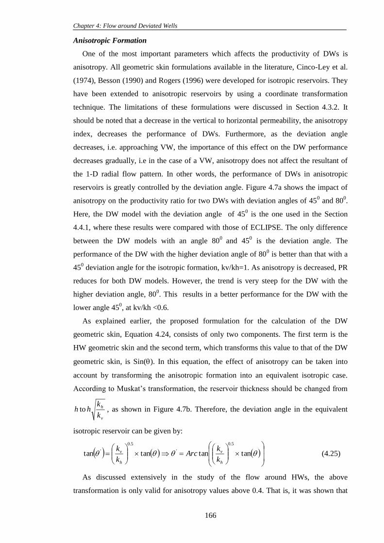
Chapter 4: Flow around Deviated Wells
166
Anisotropic Formation
One of the most important parameters which affects the productivity of DWs is
anisotropy. All geometric skin formulations available in the literature, Cinco-Ley et al.
(1974), Besson (1990) and Rogers (1996) were developed for isotropic reservoirs. They
have been extended to anisotropic reservoirs by using a coordinate transformation
technique. The limitations of these formulations were discussed in Section 4.3.2. It
should be noted that a decrease in the vertical to horizontal permeability, the anisotropy
index, decreases the performance of DWs. Furthermore, as the deviation angle
decreases, i.e. approaching VW, the importance of this effect on the DW performance
decreases gradually, i.e in the case of a VW, anisotropy does not affect the resultant of
the 1-D radial flow pattern. In other words, the performance of DWs in anisotropic
reservoirs is greatly controlled by the deviation angle. Figure 4.7a shows the impact of
anisotropy on the productivity ratio for two DWs with deviation angles of 450 and 80
0.
Here, the DW model with the deviation angle of 450 is the one used in the Section
4.4.1, where these results were compared with those of ECLIPSE. The only difference
between the DW models with an angle 800
and 450 is the deviation angle. The
performance of the DW with the higher deviation angle of 800 is better than that with a
450 deviation angle for the isotropic formation, kv/kh=1. As anisotropy is decreased, PR
reduces for both DW models. However, the trend is very steep for the DW with the
higher deviation angle, 800. This results in a better performance for the DW with the
lower angle 450, at kv/kh <0.6.
As explained earlier, the proposed formulation for the calculation of the DW
geometric skin, Equation 4.24, consists of only two components. The first term is the
HW geometric skin and the second term, which transforms this value to that of the DW
geometric skin, is Sin(). In this equation, the effect of anisotropy can be taken into
account by transforming the anisotropic formation into an equivalent isotropic case.
According to Muskat‟s transformation, the reservoir thickness should be changed from
h tov
h
k
kh , as shown in Figure 4.7b. Therefore, the deviation angle in the equivalent
isotropic reservoir can be given by:
tantan
5.0
'
h
v
k
k
tantan
5.0
'
h
v
k
kArc (4.25)
As discussed extensively in the study of the flow around HWs, the above
transformation is only valid for anisotropy values above 0.4. That is, it was shown that

Chapter 4: Flow around Deviated Wells
167
the contrast of the geometric skin calculated using the in-house simulator and the
corresponding values obtained by the equations (Joshi (1985) and Joshi-Economides
(1996)) using this transformation increases for lower anisotropy values. The same
observation was noted for the DWs with the equivalent deviation angle calculated by
Equation 4.25.
Figure 4.8 shows that the geometric skin values predicted by the in-house simulator
and Equations 4.24 and 4.25 are in good agreement for anisotropy values more than 0.1.
The AAD is only 1.3% for 480 data points (Table 4.1). However, as can be seen in
Figure 4.9, the transformation of the deviated angles using Equation 4.25 does not result
in a good approximation of the DW performance for anisotropy values lower than 0.1.
To improve this transformation Equation 4.25 was rewritten as follows:
tantan'
a
h
v
k
kArc , (4.26)
where a is a constant.
Analysis of a large number of cases showed that a should be 0.25. Thus Equation
4.25 can be written as follows:
tantan
25.0
'
h
v
k
kArc . (4.27)
Figures 4.10, 4.11 and 4.12 show that the results of the in-house simulator are in
good agreement with those obtained using Equations 4.24 and 4.27: for more than 800
data points, AAD% is only 2% (Table 4.1), , which confirms the integrity of the
proposed geometric skin correlation.
Comparing the data in Figure 4.10 with those in Figure 4.8 (with a=0.25)
demonstrates that changing the constant a does not have any effect on the DW
geometric skin for anisotropy values of above 0.4.
For the extreme case when anisotropy is zero, the flow to the wellbore is purely in
the horizontal direction (Figure 4.13), and the above set of equations (Equations 4.27,
4.24 and 4.19) correctly predicts a zero geometric skin, i.e. flow is similar to that of a
vertical well.
On the other hand, the productivity of a fully penetrating DW in a reservoir with zero
vertical permeability can be analytically given by a VW equation as follows:
w
e
DW
r
rLn
PCoskLQ
2, (4.28)

Chapter 4: Flow around Deviated Wells
168
For the fully penetrating DWs, it can be written:
CosLh , (4.29)
Substitution of the above equation into Equation 4.28 gives:
w
e
DW
r
r
PkhQ
ln
2
. (4.30)
Therefore, from both Equations 4.30 and 4.24, the geometric skin is zero, which
confirms the accuracy of the results even for the extremely highly anisotropic
reservoirs.
It should be noted that when the DW penetrates the reservoir partially, the results of
the proposed approach could be overestimated for extreme case of kv=0, if the total
formation thickness is used. That is, in this case, as vertical permeability is zero and the
flow pattern is horizontal, the projected DW is converted to a partially VW with zero
skin, which is incorrect. However, if instead of the total formation thickness, the
projected length of DW, i.e. CosL , is used for the VW flow calculation, the result
is correct. In this case, the effect of flow convergence, due to limited entry, is negligible,
as the flow is only horizontal. Therefore, reducing the formation thickness to the
projected length of the DW is valid.
4.5 SINGLE PHASE NON-DARCY FLOW
According to Darcy‟s law, Equation 4.31, the pressure drop inside a porous medium is a
linear function of velocity.
Pk
V
. (4.31)
However, this linear function is not valid for high volumetric flow rates. Forchheimer
(1914) added a quadratic term to this flow equation to express the nonlinear part of the
flow as given by:
vvVk
P
, (4.32)
From Equation 4.32, the inertial effect could be defined by a relative permeability term,
in the Darcy equation, as follows:
Vkk
PR
kre
r
1
1, (4.33)

Chapter 4: Flow around Deviated Wells
169
where eR is Reynolds number and given by:
kVRe . (4.34)
As discussed in the previous section, the flow of a DW can be defined by the flow
equation of a VW with a skin (Equation 4.1). In the case of non-Darcy flow. the total
skin is a summation of mechanical and flow skins. It should be noted that damaged skin
has not been considered in this study. Therefore, Equation 4.1 can be rewritten as
follows:
t
w
e Sr
rLn
khm
2, (4.35)
where is the pseudo pressure and St is the total skin effect that can be expressed
mathematically as follows:
ft SSS . (4.36)
In this equation, S and fS are the mechanical and flow skins, respectively. Here,
the flow skin fS represents the effect of inertia on the productivity of DWs. It should
be noticed that fS , like fS for the HWs, depends on the fluid properties and flow rates
in addition to geometrical parameters. As and fS are both functions of the volumetric
flow rate and fluid properties, obtaining fS is not a straight forward task. After
conducting a comprehensive sensitivity study it was noted that similarly to the flow
around HWs, the concept of the effective wellbore radius is the more appropriate
method to evaluate the flow skin. Hence, the concept of effective wellbore radius is
extended here to the DWs using Equation 4.37:
tS
ww err
' , (4.37)
where '
wr is the effective well bore radius, and St is the total skin factor.
Rearranging Equation 4.35 using the effective wellbore radius gives:
'
2
w
e
r
rLn
khm
. (4.38)
4.5.1 Effective Well Bore Radius Calculation by In-House Simulator
The 1-D open hole simulator developed previously for the study of flow around the
HWs has been used to evaluate the effective wellbore radius of an equivalent open hole.

Chapter 4: Flow around Deviated Wells
170
In the 1-D in-house simulator, similarly to in the 3-D in-house simulators, the flow is
steady state under the constant pressure boundary conditions at both the external and
wellbore radius. The external radius of the 1-D VW in-house simulator is that of the 3-
D DW model.
As noted earlier, the flow skin and pseudo pressure calculation are both functions of
fluid properties and flow rates. Consequently, the in-house simulator follows an
iterative procedure to estimate '
wr . The details of this procedure have been explained in
the HW Chapter, Section 3.7.
The pertinent parameters, such as geometrical parameters (the DW length, wellbore
radius, reservoir thickness and the deviation angle) are those used for developing the
geometric skin in Section 4.4, Table 4.1. Velocities were varied from 100 to 11000
m/day, to generate a large data bank required to develop a general flow skin correlation.
Two cores from the laboratory, Texas Cream and Berea cores, were used to describe the
reservoir rock. The rock properties of these two cores are listed in Table 4.2. The
reservoir fluid properties were those used for developing the geometric skin correlation
in Section 4.4. Figure 4.14, shows a good agreement between the results of the
equivalent open hole in-house simulator (EOH) with '
wr , calculated by Equations 4.37
and 4.38, and those of the HW 3-D in-house simulator. AAD% for 1350 data points is
0.1. These '
wr values are then converted to fS using Equation 4.37, to develop a skin
formulation as described in the next section.
4.5.2 Flow Skin Correlation
As noted earlier, in Section 4.5, the author benefited from the similarity of the Darcy
flow behaviour around DWs with that around HWs. Here, it is proposed to extend the
same approach adopted for modelling the flow around DWs in the case of Darcy flow to
that in the case of non-Darcy flow. Figures 4.15 and 4.16 show the isobar counter maps
around a DW with an angle 450 and a HW for the Darcy and non-Darcy flow cases,
respectively. The fluid and reservoir properties for both well models are the same. It
should be noted that a HW can be defined as a DW with a deviation angle of 900. It is
clear that for the non-Darcy flow case, as the flow approaches to the wellbore, the
velocity is increased. This results in an extra pressure drop in this region compared to
the case of Darcy flow. Therefore, the isobar counters for the non-Darcy flow are closer
to each other than those for the Darcy flow. Based on Equation 4.33, inertia affects the
single-phase gas relative permeability (krg). Figure 4.17 shows the variation of this krg

Chapter 4: Flow around Deviated Wells
171
for both horizontal and deviated wells. It is noted that krg is less than 1 near the well
bore and it reaches 1 far from the wellbore for both the HWs (Figure 4.17a) and the
DWs (Figure 4.17b).
Figure 4.18 shows the variation of the flow skin versus the deviation angle, . Here,
the reservoir thickness and the DW lengths are both 15 m. The pressure drop across the
flow models is 200 psi for the same drainage area. It seems that as the deviation
angle, , increases from 450 to 75
0, the flow skin increases gradually. This is mainly due
to the fact that flow rate increases as the deviation angle increases. Then it reaches a
plateau as the highly deviated well is converted to a HW.
These results suggest that the pertinent parameters of the flow skin of the DWs are
the same as those of the HWs. These parameters are the well length, wellbore radius,
reservoir thickness and velocity (Reynolds number). Further data analysis showed that
the same relationship reported between the geometric skin of DWs and HWs can be
extended to their flow skins. That is, the DW flow skin can be written as follows:
SinSSHWfDWf , (4.39)
where HWfS is the HW flow skin, which can be calculated using the proposed
formulation (Equation 4.40) for calculation of effective wellbore radius of the
equivalent open hole system in the HWs study in Chapter 3. It should be noted that
'
wr and total (mechanical plus flow) skin are related by Equation 4.37. After calculation
of St, Sm is deducted from St to obtain Sf required in Equation 4.39.
[b
D
D
Sm
ww
L
ha
err
Re1
' ]HW. (4.40)
with 04.0a and 6.0b .
A closer look at the data revealed that in Equation 4.39 is equal to 1.0 for all the
deviation angles.
It is noted that, based on Equation 4.39, to obtain the flow skin of a DW, first the
flow skin of a HW at the same flow conditions (the same well length, wellbore radius,
pressure drop, and reservoir characteristics) should be calculated. As discussed in the
previous Chapter, the proposed HW flow skin equation (Equation 4.40) requires an
iterative procedure as follows:
1) First, the flow skin is assumed to be zero and the effective wellbore radius is
estimated as follows:
Sm
ww err ' . (4.41)

Chapter 4: Flow around Deviated Wells
172
2) Based on the effective wellbore radius, the pressure profile and flow rate are
calculated. It should be noted that the pseudo pressure calculation is a function
of the velocity; therefore an iterative procedure is required to estimate the
pressure profile and mass flow rate.
3) Using Equation 4.40, a new effective wellbore radius is estimated, and then the
flow skin is calculated using Equation 4.37.
4) If the difference between Sf calculated with the one calculated previous step is
not negligible, the calculation is repeated from step 2, otherwise the calculated
effective well bore radius and mass flow rate are considered as the correct
answers, representing flow performance of a HW. The calculated flow skin of
the HW is then converted to that of a DW using Equation 4.39. Finally, the DW
effective radius is then calculated using Equation 4.37.
5) Based on the effective wellbore radius, the pressure profile and flow rate is
calculated.
4.5.3 Verification
Figure 4.19 shows the calculated mass flow rate obtained using Equation 4.39 and the
iterative procedure described in the previous section versus the corresponding values
obtained using the DW 3-D in-house simulator. The close agreement between these two
mass flow rates confirms the integrity of the proposed formulation and approach. In this
study AAD% average absolute deviation error for 100 data point is only 1%.
4.5.4 Application of Flow Skin
Figure 4.20 shows the productivity ratio (PR) of a DW to a VW at different deviation
angles versus velocity, which is calculated at the DW surface assuming uniform flow
along the DW surface. In order to obtain higher velocity, the wellbore pressure was
1000 psi and pressure at the external boundary was 4200 psi. The reservoir thickness
was 15 m and equal to the DW length. The Berea and Texas Cream core properties were
used to describe the reservoir rock for Figure 4.20a and 4.20b, respectively. It is noted
that for the DW with a 450 angle, PR is less than 1 at velocities above 500 m/day. At
low velocities, Darcy flow regime, the well deviation results in an improved
performance. This is more pronounced for larger well deviation angles. However, an
increase in the velocity decreases the performance of the DW, especially for smaller
well deviation angles. This indicates that when the deviated length is equal to the
reservoir thickness, the negative impact of inertia on the DW performance is more

Chapter 4: Flow around Deviated Wells
173
pronounced than that on the VW performance. This can be explained by comparing
pressure profile distribution around the DW with 450 deviation angle and around the
HW (Figures 4.15 and 4.16). It is noted that as the deviation angle increases, the isobar
counters around the wellbore become closer, which results in decreasing the affected
area by the high velocity inertial effect, thus reducing its negative impact. It was
demonstrated earlier in the HW study that the flow convergence towards the wellbore
caused an extra pressure drop around the tip of the wellbore, resulting in decreased
productivity for HWs. The same conclusion can be made here for DWs. It is noted that
the magnitude of this pressure loss decreases as the deviation angle increases. That is, as
the distance between the tip of wellbore and the reservoir boundary decreases, the flow
pattern is more linear around the tip of the wellbore, resulting in an improved DW
productivity. This observation has also been reported in the study of partial penetration
HWs. The same observation was noticed when Texas cream core properties were used
for the reservoir model description (Figure 4.20 b).
Figure 4.21 shows a comparison of the calculated PR using Berea or Texas cream
properties. It seems that the adverse effect of inertia on the DW productivity became
more pronounced compared to that on the VW productivity, when the Texas cream core
properties were used for reservoir descriptions. It is clear that the contribution of the
inertial effect depends on the term k , which is higher for Texas Cream core (Figure
4.21).
Figure 4.22 shows that the effect of the wellbore radius on PR is negligible. When
the DW length is equal to the reservoir thickness, PR decreases with velocity (Figure
4.22 a) to almost the same extent at three different wellbore radii. That is, for each of
these three cases the inertial effect is more pronounced for DW compared to VW, to the
same extent. It is interesting to note that as the DW length increases, the observed trend
changes and becomes similar to that noted for the HW Figure 4.22 b.
Figure 4.23 compares PR of Non Darcy flow with Darcy flow cases, at different
deviation angles. Here, the pressure drop across the reservoir models for all DWs, with
different deviation angles, and the VW was 3200 psi. The velocity at the DW surface
varied from 10047 to 11511 md-1
. As expected, at the lower DW length, Figure 4.23 a,
the inertial effect is more pronounced for DWs compared to VWs. That is, the PR curve
of Darcy flow is always above that of non Darcy flow. However, an increase in the DW
length changes this trend, as confirmed in Figure 4.23 b. That is, in the latter case, the
performance of DWs is better for the case of non Darcy flow, similarly to what was

Chapter 4: Flow around Deviated Wells
174
observed for HWs. This is due to the fact that the increase in the surface of the wellbore
significantly reduces the negative impact of inertia on DW performance.
The effect of the reservoir thickness was investigated by comparing the PR of a DW
with the deviated length of 45 m versus velocity at two reservoir thicknesses. As can be
seen in Figure 4.24, increasing the velocity decreases the PR. This is similar to the
observation for the DW in the reservoir model with thickness of 15 m, reported above.
It is clear that PR is always higher for the low reservoir thickness, 30 m here, because of
higher L/h, i.e. greater reservoir exposure. It is worth citing that for the case of the
reservoir thickness 45 m, because the DW length is equal to the reservoir thickness, the
PR values are close to one, i.e. deviation has minimal impact on PR. The same
observation was made for DWs with the length equal to the reservoir thickness of 15 m.
The effect of the reservoir thickness was investigated by comparing the PR of a DW
versus velocity at two reservoir thicknesses, Figure 4.25. Here, DW length is equal to
the reservoir thickness. As noted in this Figure, increasing the velocity decreases the
PR. It seems that the impact of inertia on DW productivity compared to that on VW is
more pronounced for thicker reservoirs.
4.6 GAS CONDENSATE FLOW
As mentioned earlier, the aim was to extend the single-phase mathematical
modelling approach to study two-phase flow of gas and condensate around DWs. To
achieve this objective, an in-house simulator was developed, simulating a steady state
flow of gas and condensate around a single DW. In the in-house simulator, the
generalised relative permeability correlation (Jamiolahmady et al. 2009) was employed,
which accounts for the combined effects of positive coupling and negative inertia on kr.
To confirm the integrity of the structure of the in-house simulator, some of the
simulations conducted using the in-house simulator were also performed using the fine
grid option of the ECLIPSE 300 commercial software. Next, an extensive bank of data
was generated using the in-house simulator. This data bank was then used to propose a
general method for modelling the two-phase flow of gas and condensate around DWs,
using an equivalent open hole approach.
4.6.1 In-House 3-D Two-Phase Deviated Well Model
Chapter 4: Flow around Deviated Wells
175
The 3-D geometry which is used to simulate the gas condensate flow around a DW
is the same as that for the single phase flow case (Figure 4.1). However, the governing
equations are those describing two-phase flow of gas and condensate.
Governing Equations
As mentioned earlier, the two equations describing the two-phase flow of gas and
condensate around a DW are similar to those described for gas condensate flow around
a HW:
The continuity equation for gas and condensate flow at steady state conditions
0. cg vv , (4.42)
where g and c represent the gas and condensate phases, respectively.
1) The flow equation for each phase:
Pkk
vi
ri
i
. i=g,c (4.43)
Combining the continuity and flow equations, after some mathematical manipulation,
gives:
0.
Pk
kk
c
r
g
r
. (4.44)
As the fluids flow through the porous media, there is a mass transfer between the
two phases but the total fluid composition (zj) is constant (Fevang &Whitson (1996)), as
expressed by the following equation.
.)1(
)1(cons
GTRGTR
GTRxGTRyz
cg
jcjg
j
, (4.45)
where GTR is the total gas fractional flow. A binary mixture of C1 (methane) and n-C4
(normal butane) has been used as the gas-condensate fluid model. The values of
-nC4
binary gas condensate model mixture as a function of pressure are those measured in the
hydrocarbon carbon recovery group‟s laboratory as well as in literature data (Sage et. al,
1940; SUPERTRAPP User‟s Guide, 1992; Weinaug and Katz, 1943) at 311 K over a
wide pressure range, which were implemented in the model in a tabular form.
Mathematical Solution Technique
Similarly to the single-phase modelling approach, the governing non-linear partial
differential equation (PDE), Equation 4.44, and the auxiliary equation, Equation 4.45,
are solved using Comsol multi-physic software (Version 3.5, 2008), which uses the

Chapter 4: Flow around Deviated Wells
176
finite element method. The main dependent variable in this equation is P (pressure) but
the equations are solved for both pressure and GTR.
The boundary conditions applied to this system are:
1) The pressure at the outer boundary (external radius) is known.
2) The pressure at the inner boundary (wellbore radius) is known.
3) The pressure gradient in the wellbore has been ignored, i.e. infinite conductivity
for the flow through DW wellbore.
3) As noted earlier, the total composition is constant, Equation 4.45. Therefore,
either the total composition fluid is given or GTR at a particular point in the drainage
area, normally at the wellbore, should be known and used in Equation 4.45 to calculate
the total composition.
4.6.2 ECLIPSE 3-D Two-Phase Deviated Well Model
The accuracy of the two-phase mathematical in-house simulator was confirmed by
comparing its results with those of ECLIPSE300 under the same prevailing flow
conditions.
The reservoir model in this exercise has the core properties of Texas Cream with
porosity 0.21 and permeability 9.1 mD. The reservoir fluid is a binary mixture of C1
(methane) and n-C4 (normal butane) described in the previous section. The reservoir is
38 m in the x and y directions and 4 m in the z direction. The length of the DW is 15 m.
Many different cases were simulated using both ECLIPSE300 with a fine grid option
and the in-house simulator. The fractional flow at average reservoir pressure was the
same in both simulators. As the kr correlations used in these two models (i.e. Comsol
and ECLIPSE300 models) are different, the base curve relative permeability has been
used to describe the flow around a DW in these simulations.
In ECLIPSE 300, seventy injection wells were placed at the boundary of the
reservoir to keep the reservoir pressure at the drainage boundary constant.
Figure 4.26 shows the good agreement between the results of two simulators. The
arithmetic average absolute percentage deviation (AAD%) of the predicted mass flow
rates values by the ECLIPSE300 simulator compared to those estimated by the DW
simulator was 2 %. The wellbore pressure was constant and equal to 1365 psi in these
simulations. The only difference between runs 1 and 2 corresponding to each DW was
the reservoir pressure, with the corresponding values being 1765 and 1565 psi,
respectively.
Chapter 4: Flow around Deviated Wells
177
4.6.3 In-House 1-D Two-Phase Open-Hole Well Model
The 1-D two-phase open-hole in-house simulator is the one, which was developed to
simulate the steady state two-phase flow of gas and condensate around a single VW in
the HW study, Chapter 3. As noted in the previous chapter, the model features are
similar to those of the single-phase flow model, but instead, the governing equations of
the two-phase flow of gas and condensate, as described above, are solved.
4.6.4 Effective Wellbore Radius
The total (gas and condensate) mass flow rate of DWs can be calculated using an
equivalent open-hole (EOH) vertical well as follows:
'
0
2
w
e
Pe
Pw g
rgg
l
rll
r
rLn
dpkk
kh
m
, (4.46)
where '
wr is the effective wellbore radius calculated by Equation 4.37. As noted
earlier, tS , total skin, given by Equation 4.36 is the summation of mechanical and flow
skins, neglecting damage skin. mS depends on the geometrical parameters and
anisotropy. fS is defined as the difference between the effect of two-phase flow
behaviour around DW and EOH VW systems. Here, the author intends to introduce an
EOH system which produces the same flow performance, gas and condensate
production rate, as that of a DW system. An approach similar to that used for the single-
phase flow system described in Section 4.5.1 has been followed. That is, the mass flow
rates of the 1-D open-hole simulator and that of the 3-D in-house simulators are
matched iteratively by varying '
wr . '
wr is then converted to Sf using Equation 4.37.
Using the in-house simulators, a large bank of data was generated to obtain two
phase flow skin for different flow conditions. For this part of study, the Texas Cream
core properties described the reservoir rock. The fluid was a binary mixture of C1
(methane) and n-C4 (normal butane). The reservoir and wellbore pressures were varied
between 1800 psi to 1750 psi and 700 psi to 400 psi, respectively. GTR was changed
from 0.846 to 0.999.
In the previous section, the non-Darcy and Darcy flow study, it was demonstrated
that the mechanical and single-phase flow skin of a DW could be estimated by using a
simple relation between the corresponding skin values calculated for a HW and the

Chapter 4: Flow around Deviated Wells
178
deviation angle (Equations 4.24 and 4.39). Here a similar formulation is proposed for
the two-phase flow skin:
SinSSHWfDWf , (4.49)
The results of the data analysis showed that the constant in Equation 4.49 should
be 1. In other words, the transformation of the two-phase flow skin formulation of HWs
to that of DWs is similar to that for the single-phase flow and geometric skin cases.
Figure 4.27 shows the mass flow rate calculated using the two-phase flow skin
correlation based on the effective radius concept (Equation 4.49) versus the
corresponding values obtained by using the in-house simulator. It is noted that the
results of the DW matches exactly those of EOH, using the two-phase flow skin
correlation, Equation 4.49. AAD% for 40 data points is 1%, which confirms the
accuracy of the proposed formulation and method.
4.6.5 Application of Effective Wellbore Radius
As mentioned before, the impact of inclination can be quantified by introducing a
skin factor. The geometric skin value is negative, as the performance of a DW is better
than that of a VW. In the case of single-phase non-Darcy flow, the flow skin expresses
the difference between the inertial effect on the DW and EOH VW systems, based on
the geometric skin. It should be mentioned that this flow skin is always positive, that is,
the impact of inertia is always more pronounced for a DW compared to an EOH VW
system. Here, the velocity around the EOH is decreased significantly as the surface is
increasing significantly compared to DWs. The gas condensate flow behaviour around
DWs is more complex because the relative permeability of gas and condensate is a
function of velocity as well as IFT. That is, inertia decreases the relative permeability,
whilst coupling increases it.
Figure 4.28 shows the variation of the two-phase skin versus the deviation angle at
three different gas fractional flows at the wellbore (GTRwell). The formation thickness,
the wellbore length and the wellbore radius are 15, 15, and 0.07 m, respectively. The
rock properties were those of the Texas Cream core, Table 4.2. The reservoir pressure is
constant for all different cases considered here while the wellbore pressure is varied to
obtain different GTRwell and velocity. It is noted that the absolute value of the two-phase
flow skin decreases as the inclination angle decreases. For the same pressure drop, as
the deviation angle decreases the DW flow rate decreases, which at lower GTRwell
values, in turn, could also result in reducing the positive impact of coupling for the DW.
At higher GTRwell values, the impact of inertia on the relative permeability is more

Chapter 4: Flow around Deviated Wells
179
pronounced, i.e. increasing GTR decreases the absolute value of the-two phase flow
skin.
Figures 4.29 to 4.31 show PR, ratio of flow rates for the given pressure drop of a
deviated to a vertical well versus deviation angle. In this exercise, the DW and VW had
the same L, rw ,with kr varying due to coupling and inertia. For the set of simulation
runs shown in these figures, the pressure drop across the reservoir and wellbore pressure
were either 50 or 1800 psi. The DWs length and reservoir thickness were both 15 m,
and the Texas Cream core properties (Table 4.2) were used unless otherwise stated.
Figure 4.29 compares PR versus the deviation angle at three different GTRw. It is
noted, as expected, that the PR increases by increasing the deviation angle. Decreasing
GTRw, improves the PR for all DWs considerably. This is mainly due to the more
pronounced impact of positive coupling in DWs compared to that in VWs.
Figure 4.30 presents the effect of the wellbore radius on PR versus the deviation
angle. Here, GTRw was 0.7. As can be seen the impact of the wellbore radius on the
DW performance is minimal. The small increase in PR as rw increases is due to the
higher surface flow area in the HW model at this low GTR value.
The impact of the reservoir thickness on the PR is shown in Figure 4.31. Here again,
GTRw was 0.7. The same conclusion that has been drawn for the HWs study can be
made here: that is, the performance of DWs is better for thin reservoirs.
Figure 4.32 examines the effects of the rock properties on the PR versus the
deviation angle. Two different rocks, Berea and Texas Cream, were used here. The rock
properties of theses two cores are listed in Table 4.2. The wellbore pressure and the
differential pressure across the reservoir models were 1565 and 200 psi. The velocities
for the DW models with Texas Cream and Berea core properties were varied from 17,
156 to 134, 1400 md-1
, respectively. The observed trends for both models are the same,
i.e. increasing GTRw decreases the PR significantly because of dominant impact of
inertia for DWs or, in other words, there is a more pronounced coupling effect for VW
at lower GTRw. It should be noted that in these simulations, the DW lengths were equal
to the reservoir thickness. The observed trends here are in the opposite direction to those
reported for the HWs, where velocity at the HWs surface decreased significantly,
resulting on a decrease in the pronounced impact of inertia on the HWs productivity. As
will be shown here, Figure 4.36, for the DWs with a length longer than the reservoir
thickness, the observed trend is similar to that for HWs .It should be noted that for the
same pressure drop, higher velocity in Berea results in a more pronounced effect of
inertia in VWs, slightly increasing the PR for this rock compared to that for Texas

Chapter 4: Flow around Deviated Wells
180
Cream. It should be noted that k of Texas Cream is higher than that of Berea, which
at same velocity would results in a more pronounced impact of inertia in Texas Cream
compared to that in Berea.
Figure 4.33 shows the PR versus the deviation angle at three different p of 100,
200 and 400 psi. The wellbore pressure was either 1365 (Figure 4.22 a) or 1450 (Figure
4.22 b) psi. GTRw was 0.7. The corresponding VW velocity values for the three
drawdown pressure of Figure 4.33a, were 6, 11, and 27 md-1.
, respectively. The
corresponding values for the data in Figure 4.33b were 6, 13, and 39md-1
, respectively.
It should be noted that increasing the velocity results in an increase of the negative
inertial effect on the productivity of VW. That is, the PR increases as the velocity is
increased.
Figure 4.34 shows PR versus GTRw for a DW with 15 m length, at different
deviation angles, in the reservoir model with thickness 15 m. The well and reservoir
pressures were 1725 and 1775 psi, respectively. The velocity at VW surface varied from
3.6 to 33 md-1
. It is noted that, as the deviation angle increases, the PR increases for all
GTRw. Furthermore, the PR remains almost constant when GTRw varies between 0.7 to
0.85. However, PR decreases at higher GTRw values (greater than 0.95) where the
negative inertial effect is more pronounced for the DW compared to the VW.
The impact of DW length on PR is displayed in Figure 4.35. For this set of data,
GTRw was 0.7. The rate of increase of the PR with increase in the deviation angle is
more or less similar for all DW lengths. It is interesting to point out that increasing the
DWs length significantly improved the PR. For example, if the DWs length increased
from 30 to 60 m, the PR increased considerably, i.e. by a factor of 2. It should be noted
that in these simulations, the DW length can be increased until the DW fully penetrates
the whole 15 m thickness of the formation.
The PR of a DW with deviation angle of 870 versus the DW lengths at different
GTRw is shown in Figure 4.36. In these simulations, the wellbore and differential
pressures were 1725 and 40 psi. The velocity of the VW varied from 0.28 to 3.9 m/day.
As expected, increasing the DW length significantly improves the performance of the
DW. Moreover, the performance of DWs is better at high GTRw values compared to
that for low GTRw values. This is mainly due to the more pronounced adverse effect of
inertia on the productivity of VWs, compared to that of DWs, at higher GTRw values. It
should be noted that, as the DW length increases, the velocity decreases, which in turn
decreases the negative impact of inertia on the productivity of DWs compared to that of

Chapter 4: Flow around Deviated Wells
181
VWs. It is also important to point out that as GTRw approaches 1, the gas fractional
flow and flow rate increases significantly due to the high mobility of gas.
A comparison of data in Figures 4.34 and 4.36 demonstrates that the PR strongly
depends on the DW lengths. It is noted that the trends of PRs for long and short DWs
are in the opposite direction. That is, in the former, an increase in GTRw has increased
the negative impact of inertia on the DW performance more, compared to that of the
VW, (PR decreases at higher GTRw). This results in the latter the velocity of long DWs
decreases significantly compared to that of a VW e.g. this results in a decrease in the
negative impact of inertia on the DW performance, compared to that of the VW, (PR
increases at higher GTRw).
4.7 SUMMARY AND CONCLUSIONS
A number of in-house simulators were developed to study the well performance of
deviated wells (DWs) in gas and gas condensate reservoirs. The integrity of the results
of the in-house simulators was confirmed by comparing some of their results with those
obtained using ECLIPSE with fine grid for the same prevailing flow conditions.
1. It was confirmed that at low velocities, Darcy flow regime, any well deviation
from vertical results in an improved performance, i.e. there is a negative geometric
skin.
2. A comprehensive study for some of equations for DWs available in the literature
has been conducted and the range of their application has been determined. The
results indicated that these equations cannot accurately predict DWs productivity in
an anisotropic formation with anisotropy values less than 0.6.
3. It was shown that the DWs geometric skin depends on the same pertinent
parameters as those for horizontal wells (HWs), i.e., length of horizontal well,
radius of the well, reservoir thickness, and anisotropy. Therefore, an easy to use
formulation for geometric skin of DWs was developed, which correlated the HWs
geometric skin to that of DWs, using the deviation angle. The integrity of the
geometric skin formulation was validated by comparing its results for data points
not used in its development.
4. Similarly to that of geometric skin, the single-phase flow skin formulation for
DWs was developed, which is related to that for HWs. Based on this formulation,
first an effective wellbore radius of an equivalent open-hole system should be
estimated for the HW with the same well length. Then, this effective wellbore

Chapter 4: Flow around Deviated Wells
182
radius is converted to the HW flow skin to be included in the proposed formulation
to calculate the DW flow skin. This flow skin is then converted to an effective
radius to be used in an open-hole well model replicating flow around the
corresponding DW. The integrity of the flow skin formulation was validated by
comparing its predictions with the corresponding estimated values using the in-
house simulator, thereby confirming the integrity of the proposed approach.
5. A comprehensive sensitivity study has been also conducted on the impact of
important parameters on PR of DW to (vertical well) VW for single phase. From
these results the following conclusions can be made:
6. For the same DW length, as that of a VW (i) an increase in velocity decreases
the PR (of the DW to the VW), due to the more pronounced effect of inertia for the
DW compared to that for the VW, especially for smaller well deviation angles; (ii)
the PR is always higher for low reservoir thickness values: (iii) the negative impact
of inertia on DW productivity compared to that on VW productivity is more
pronounced for thicker reservoirs, due to the higher production rate.
7. Similarly to the HW findings at higher DW length, the negative impact of inertia
is less for DWs compared to that for VW, thus improving the PR, especially at
higher velocities.
8. In the case of a two-phase flow of gas and condensate, a similar approach to that
for the single-phase non-Darcy flow skin has been followed to develop the two-
phase flow skin for the DWs. The integrity of the proposed procedure has been
confirmed by comparing its predictions with the corresponding estimated values
using the in-house simulator .
9. The results of a comprehensive sensitive study on the impact of parameters on
the PR of DWs to VWs for two-phase gas condensate demonstrated that:
10. For the same DW length, as that of the VW (i) as the deviation angle increases,
PR increases for all GTRw (gas fractional flow at the wellbore), due to higher
negative geometric skin, (ii) decreasing GTRw below 0.95 improves the PR because
of the more pronounced effect of positive coupling in DWs compared to that in
VWs, but the extent of this improvement is almost constant when GTRw varies
between 0.7 to 0.85 (iii) the PR decreases at GTRw values greater than 0.95, where
the negative impact of inertia is more pronounced for a DW compared to that for a
VW (iv) the DW performance is better for thinner reservoirs.
11. Similarly to the HW cases, (i) PR strongly depends on the DW lengths: higher L
means higher PR, (ii) at higher DW lengths, the negative impact of inertia is less for

Chapter 4: Flow around Deviated Wells
183
DWs compared to that for VWs, improving the PR, especially at higher velocities
(iii) wellbore radius has minimal impact on DW performance.
12. At higher GTRw, the trends of variation of PR for long and short DWs are in
opposite directions. That is, in the former, an increase in GTRw increases the
negative impact of inertia on the DW performance more than in the case of a VW,
where PR decreases at higher GTRw. However in the latter, the velocity of long
DWs decreases significantly compared to that of a VW, resulting in a decrease in
the negative impact of inertia on the DW performance compared to that of VW
where the PR increases at higher GTRw.

Chapter 4: Flow around Deviated Wells
184
References
Besson, J., 22-24 Oct. 1990: Performance of Slanted and Horizontal Wells on
Anisotropic Medium, SPE 20965, Presented at Europec 90, The Hague, the
Netherlands.
Chen G., Tehrani D.H. and Peden J., 12-15 February 1995: Calculation of Well
Productivity in a Reservoir Simulator I, SPE29121, Presented at the 1995 SPE
Symposium on Reservoir Simulation in San Antonio, Texas.
Cinco-Lay H., Ramey H. J. Jr. and Miller, F. G. , 28 Sept-1 Oct. 1975: Pseudo Skin
Factors for Partially Penetrating Directionally-Drilled Wells, SPE 5589, Presented at the
50th
Annual Fall Meeting of the SPE of AIME, Dallas, Texas.
Cinco-Lay H., Ramey H. J. Jr. and Miller F. G., 1975: Unsteady State Pressure
Distribution Created by a Directional Drilled Well, p 1392-1400, JPT.
Comsol Multiphysics Reference Manuals http://www.comsol.com, version 3.4, 2008,
by COMSOL, Inc.
Economides M.J., Deimbacher F. X., Clement W. B. and Heinmann E. Z. , Dec 1991:
Comprehensive Simulation of Horizontal Well Performance, SPE 20717.
Economides M.J., Brand C.W. and Frick, T.P., Dec. 1996: Well Configurations in
Anisotropic Reservoirs, SPEFE (Dec. 1996), 257-262. (Also Paper SPE 27980, 1994.)
Fevang Ø. And Whitson C.H., 1996: Modeling Gas-Condensate Well Deliverability,
SPE reservoir engineering.
Forchheimer P., 1914: Hydraulik, Chapter15, pp. 116-8, Leipzik and Berlin.
'Gas Condensate Recovery Project', Progress Report, Sep 2008-Feb 2009, Heriot-Watt
University, Institute of Petroleum Engineering.
'Gas Condensate Recovery Project', Final Report FTPM/02/2-2, July 2005-2008, Heriot-
Watt University, Institute of Petroleum Engineering.
Giger, F., May 1985: Reduction du nombre de puits pm I‟tilisation de forages
horizontals, Reveue de L‟institute Gancais du Petrole, 38.
Jamiolahmady M., Sohrabi M., Ireland S., and Ghahri P., 2009: A Generalized
Correlation for Predicting Gas-Condensate Relative Permeability at near the Wellbore
Conditions, Journal of Petroleum Science and Engineering.
Joshi S.D., 1991: Horizontal Well Technology, PennWell, Tulsa, Oklahoma.
Rogers, E. and Economides M., Nov. 1996: The Skin due to Slant of Deviated Wells in
Permeability- Anisotropic Reservoirs, SPE37068.

Chapter 4: Flow around Deviated Wells
185
Sage B.H, Hick B.L. and Lacey W.N. , 1940: Phase Equilibria in hydrocarbon system-
the methane-n-butane systems in the two-phase region, Ind. Eng. Chem. 32, 1058-1092.
SUPERTRAPP (NIST Thermophysical Properties of Hydrocarbon Mixture Database)
User„s Guide by National Institute of Standards and Technology (NIST), NIST
Standard Reference Database 4, July 1992, Version 1.0.
Suk Kynoon Choi, Liang-Biao Ouyang, and Wann-Sheng Huang, 21-24 Sep. 2008: A
Comprehensive Comparative Study on Analytical PI/PR Correlations, SPE 116580,
Presented SPE Annual Technical Conference and Exhibition held in Denver, Colorado,
USA.
Tehrani D.H., Chen G. and Peden, J. M., 10-12 December 1995: Effect Absolute
Permeability of a Heterogeneous Reservoir for Calculating Well Pressure, Presented at
the SPE & UAE University Regional Symposium on Improved Oil Recovery, in Al-
Ain, UAE.
Weinage C.F. and Katz D.L., 1943: Surface Tension of Methane-Propane Mixtures,
Industrial Engineering Chem. 35(2), 239-246.

Chapter 4: Flow around Deviated Wells
186
Table 4.1: Parameters of deviated well models in this study.
Length of deviated well (DW) 15-720 m 15-720 m
Deviation angle 0-87 0 0-87 0
Reservoir thickness 15-45 m 15-45 m
Wellbore radius 0.07-0.21 m 0.07-0.21 m
Anisotropy
h
v
k
k 0.01-1.0 0.01-1.0
Table 4.2: Basic core properties. Type core
Porosity Permeability
(mD)
Single-phase
inertia factor (1/m)
Texas Cream 0.21 11.1 3.93E+9
Berea 0.185 100 1.08E+8

Chapter 4: Flow around Deviated Wells
187
Figure 4.1: A schematic diagram of the deviated well model in this study.
0
1
2
3
4
5
6
7
0 1 2 3 4 5 6 7
Mass flow rate (kg/s)-ECLIPSE
Mas
s fl
ow
rat
e (k
g/s
)-C
om
sol
456580
Deviation angle
Figure 4.2: Comparison of the results of ECLIPSE single phase deviated well models
with deviation angles of 450, 65
0, and 80
0 at three different pressure drops with those of
the in-house simulator under the same prevailing conditions.
h
Xres

Chapter 4: Flow around Deviated Wells
188
0.7
0.8
0.9
1
1.1
1.2
1.3
0 0.2 0.4 0.6 0.8 1kv/kh
PR
(D
W/V
W)
Comsol
ECLIPSE
DW-450
Figure 4.3a: Ratio of deviated to vertical well flow rates, for the same pressure drop,
estimated by the in-house and ECLIPSE single deviated well models, 450
well deviation
angle.
0.8
0.9
1
1.1
1.2
1.3
1.4
0 0.2 0.4 0.6 0.8 1kv/kh
PR
(D
W/V
W)
Comsol
ECLIPSE
Cinco-Ley
Besson
Rogers
DW-450
Figure 4.3b: Ratio of deviated to vertical well flow rates, for the same pressure drop,
estimated by the in-house simulator (single phase deviated well model) and those
obtained by the Cinco et. al, (1975), Besson (1990) and Rogers et. al (1996) correlations
versus formation anisotropy, 450
well deviation angle.

Chapter 4: Flow around Deviated Wells
189
(a)
(b)
Figure 4.4: Pressure counter maps around two deviated wells; a) 045 ; b) 080 .

Chapter 4: Flow around Deviated Wells
190
Figure 4.5: Pressure counter map around a horizontal well.
0
1
2
3
4
5
6
0 1 2 3 4 5 6Sm-In-house Simulator
Sm
-Est
imat
ed C
orr
elat
ion
Figure 4.6: Geometric skin of deviated wells (with parameters described in Table 4.1),
calculated using Equation 4.24, versus the corresponding values obtained by applying
the calculated in-house simulator mass flow rates into Equation 4.19, isotropic
formation.

Chapter 4: Flow around Deviated Wells
191
0
0.2
0.4
0.6
0.8
1
1.2
1.4
0 0.2 0.4 0.6 0.8 1
kv/kh
PR
(D
W/V
R)
45
80
DW-θ
Figure 4.7a: Ratio of deviated to vertical well flow rates, for the same pressure drop,
estimated by the in-house simulator (single phase deviated well model) versus
formation anisotropy for two deviation angles of 450
and 800.
Figure 4.7b: A schematic diagram of the deviated well in the equivalent isotropic
reservoir.
x
' '
v
h
k
kh
SinL
L
z
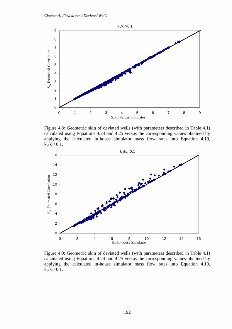
Chapter 4: Flow around Deviated Wells
192
kv/kh>0.1
0
1
2
3
4
5
6
7
8
9
0 1 2 3 4 5 6 7 8 9
Sm-In-house Simulator
Sm
-Est
imat
ed C
orr
elat
ion
Figure 4.8: Geometric skin of deviated wells (with parameters described in Table 4.1)
calculated using Equations 4.24 and 4.25 versus the corresponding values obtained by
applying the calculated in-house simulator mass flow rates into Equation 4.19,
kv/kh>0.1.
kv/kh=0.1
0
2
4
6
8
10
12
14
16
0 2 4 6 8 10 12 14 16Sm-In-house Simulator
Sm
-Est
imat
ed C
orr
elat
ion
Figure 4.9: Geometric skin of deviated wells (with parameters described in Table 4.1)
calculated using Equations 4.24 and 4.25 versus the corresponding values obtained by
applying the calculated in-house simulator mass flow rates into Equation 4.19,
kv/kh=0.1.

Chapter 4: Flow around Deviated Wells
193
kv/kh>0.1
0
1
2
3
4
5
6
7
8
9
0 1 2 3 4 5 6 7 8 9
Sm-In-house Simulator
Sm
-Est
imat
ed C
orr
elat
ion
Figure 4.10: Geometric skin of deviated wells (with parameters described in Table 4.1)
calculated using Equations 4.24 and 4.27 versus the corresponding values obtained by
applying the calculated in-house simulator mass flow rates into Equation 4.19,
kv/kh>0.1.
kv/kh=0.1
0
2
4
6
8
10
12
14
16
0 2 4 6 8 10 12 14 16Sm-In-house Simulator
Sm
-Est
imat
ed C
orr
elat
ion
Figure 4.11: Geometric skin of deviated wells (with parameters described in Table 4.1)
calculated using Equations 4.24 and 4.27 versus the corresponding values obtained by
applying the calculated in-house simulator mass flow rates into Equation 4.19,
kv/kh=0.1.

Chapter 4: Flow around Deviated Wells
194
kv/kh=0.01
0
5
10
15
20
25
30
35
0 5 10 15 20 25 30 35Sm-In-house Simulator
Sm
-Est
imat
ed C
orr
elat
ion
Figure 4.12: Geometric skin of deviated wells (with parameters described in Table 4.1)
calculated using Equations 4.24 and 4.27 versus the corresponding values obtained by
applying the calculated in-house simulator mass flow rates into Equation 4.19,
kv/kh=0.01.
Figure 4.13: Flow pattern around a deviated well in the reservoir with a zero vertical
permeability, kv=0 .
x
CosL
L
h
z

Chapter 4: Flow around Deviated Wells
195
0
200
400
600
800
1000
1200
1400
1600
1800
0 500 1000 1500
Mass Flow Rate(kg/s)-In house simulator
Mas
s F
low
Rat
e (k
g/s
)-E
OH
(a)
0
5
10
15
20
25
30
0 5 10 15 20 25 30
Mass Flow Rate (kg/s)
HW-In house simulator
Mas
s F
low
Rat
e(kg/s
)
EO
H I
n-h
ouse
sim
ula
tor
(b)
Figure 4.14: Calculated mass flow rates using EOH model with equivalent radius versus
the corresponding values estimated by the DW-in house simulator, (a) Berea (b) Texas
Cream core properties (listed in Table 4.2).

Chapter 4: Flow around Deviated Wells
196
(a)
(b)
Figure 4.15: Isobar curves around a deviated well with a 450 angle a) without (Darcy
flow) b) with inertia (Non-Darcy flow)
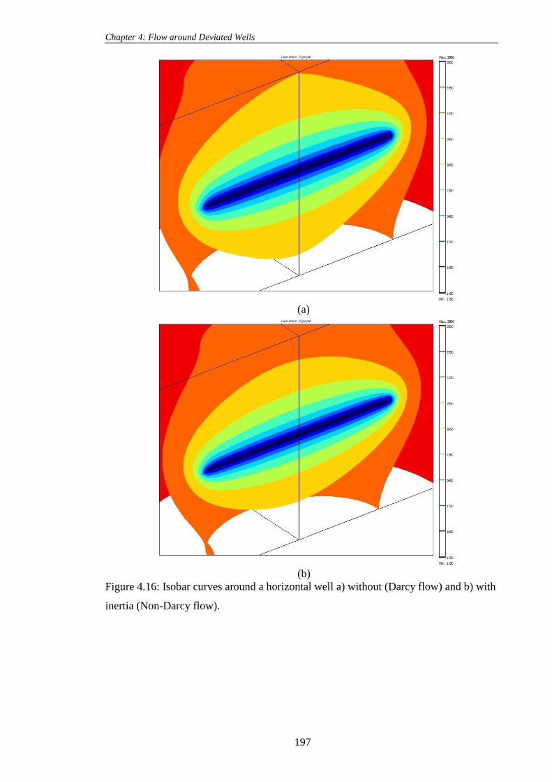
Chapter 4: Flow around Deviated Wells
197
(a)
(b)
Figure 4.16: Isobar curves around a horizontal well a) without (Darcy flow) and b) with
inertia (Non-Darcy flow).

Chapter 4: Flow around Deviated Wells
198
(a)
(b)
Figure 4.17: rk profiles for non-Darcy (inertial) flow around a) horizontal well and b)
deviated well (with 450 angles).

Chapter 4: Flow around Deviated Wells
199
0.3
0.32
0.34
0.36
0.38
0.4
0.42
0.44
0.46
0.48
0.5
40 50 60 70 80 90Teta
Sf
Figure 4.18: Variation of flow skin versus Theta ( ), the pressure drop across the flow
domain is 200 psi, h=LDW=15 m, rw= 0.07 m.
0
50
100
150
200
250
0 50 100 150 200 250
Mass Flow Rate(kg/s)-In house simulator
Mas
s F
low
Rat
e(k
g/s
)-E
OH
Figure 4.19: Mass flow rates calculated using the flow skin correlation based on the
author„s proposed the effective wellbore radius correlation versus the corresponding
values obtained by the in-house simulator, single-phase non-Darcy flow.

Chapter 4: Flow around Deviated Wells
200
0.9
0.95
1
1.05
1.1
1.15
0 2000 4000 6000 8000 10000 12000 14000
Velocity at DW Surface (m/day)
PR
(DW
/VW
)
45
60
75
80
84
87
90
Teta(Degree)
(a)
0.95
0.97
0.99
1.01
1.03
1.05
1.07
1.09
1.11
1.13
1.15
0 500 1000 1500 2000 2500
Velocity at DW Surface (m/day)
PR
(DW
/VW
)
45
60
75
80
84
87
90
Teta(Degree)
(b)
Figure 4.20: Productivity ratio (deviated to vertical well) (PR) versus velocity at
different deviation angles, rw=0.07 m, h=15 m , Pw=1000 psi a) Berea b)Texas Cream
(core properties listed in Table 4.2).
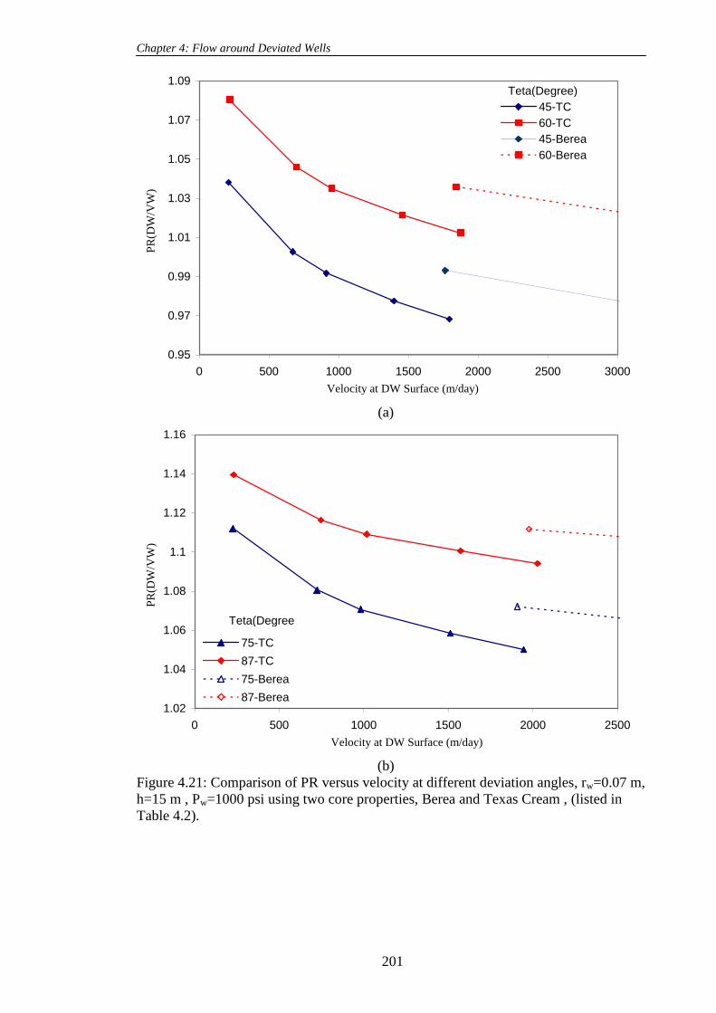
Chapter 4: Flow around Deviated Wells
201
0.95
0.97
0.99
1.01
1.03
1.05
1.07
1.09
0 500 1000 1500 2000 2500 3000
Velocity at DW Surface (m/day)
PR
(DW
/VW
)
45-TC
60-TC
45-Berea
60-Berea
Teta(Degree)
(a)
1.02
1.04
1.06
1.08
1.1
1.12
1.14
1.16
0 500 1000 1500 2000 2500
Velocity at DW Surface (m/day)
PR
(DW
/VW
)
75-TC
87-TC
75-Berea
87-Berea
Teta(Degree
(b)
Figure 4.21: Comparison of PR versus velocity at different deviation angles, rw=0.07 m,
h=15 m , Pw=1000 psi using two core properties, Berea and Texas Cream , (listed in
Table 4.2).

Chapter 4: Flow around Deviated Wells
202
0.95
0.97
0.99
1.01
1.03
1.05
1.07
1.09
1.11
0 2000 4000 6000 8000 10000 12000
Velocity at DW Surface (m/day)
PR
(DW
/VW
)
0.070.140.21
rw(m)
(a)
2.5
2.55
2.6
2.65
2.7
2.75
2.8
2.85
2.9
0 2000 4000 6000 8000 10000 12000
Velocity at DW Surface (m/day)
PR
(DW
/VW
)
0.070.140.21
rw(m)
(b)
Figure 4.22: Productivity ratio (deviated to vertical well) versus velocity (at the DW
surface) at three wellbore radii, h=15 m, Pw=1000 psi, Teta= 600 a) L=15 m and b)
L=45 m.

Chapter 4: Flow around Deviated Wells
203
0.9
0.95
1
1.05
1.1
1.15
1.2
30 40 50 60 70 80 90
Teta (Degree)
PR
(DW
/VW
)
Darcy Flow
Non Darcy Flow
(a)
2.5
2.55
2.6
2.65
2.7
2.75
2.8
2.85
2.9
70 75 80 85 90
Teta (Degree)
PR
(DW
/VW
)
Darcy Flow
Non Darcy Flow
(b)
Figure 4.23: Productivity ratio (deviated to vertical well) versus the deviation angle for
Darcy and non Darcy flow regimes, rw=0.07 m, h=15 m, Pw=1000 psi and Pres= 4200 psi
a) LDW=15 m b) LDW=45 m, Berea core properties, listed in Table 4.2.

Chapter 4: Flow around Deviated Wells
204
0.9
1
1.1
1.2
1.3
1.4
1.5
0 2000 4000 6000 8000 10000 12000
Velocity at the DW Surface (m/day)
PR
(DW
/VW
)
30
45
h(m)
(a)
0.9
1
1.1
1.2
1.3
1.4
1.5
1.6
0 2000 4000 6000 8000 10000 12000
Velocity at the DW Surface (m/day)
PR
(DW
/VW
)
30
45
h(m)
(b)
Figure 4.24: Productivity ratio (deviated to vertical well) versus velocity (at the DW
surface) two formation thicknesses, Pw=1000 psi, LDW=45 m a) Theta= 600 b) Theta=
840
.

Chapter 4: Flow around Deviated Wells
205
0.9
0.92
0.94
0.96
0.98
1
1.02
0 2000 4000 6000 8000 10000 12000
Velocity at the DW Surface (m/day)
PR
(DW
/VW
)
30
45
h(m)
(a)
0.95
0.97
0.99
1.01
1.03
1.05
1.07
1.09
0 2000 4000 6000 8000 10000 12000
Velocity at the DW Surface (m/day)
PR
(DW
/VW
)
30
45
h(m)
(b)
Figure 4.25: Productivity ratio (deviated to vertical well) versus velocity for two
different reservoir thickness values, Pw=1000 psi, LDW =h a) Theta= 600 b) Theta= 84
0.

Chapter 4: Flow around Deviated Wells
206
0
0.05
0.1
0.15
0.2
0.25
0.3
0.35
0.4
0.45
0.5
0 0.1 0.2 0.3 0.4 0.5Mass flow rate (kg/s)-ECLIPSE
Mas
s fl
ow
rat
e (k
g/s
)-C
om
sol
8045
Deviation angle
Figure 4.26: Comparison of the results of ECLIPSE two-phase deviated well models
with deviation angles of 800 and 45
0 with those of the in-house simulator at two
different pressure drops of 200 and 400 psi.
0
0.5
1
1.5
2
2.5
3
0 0.5 1 1.5 2 2.5 3
Mass Flow Rate (kg/s)-In house Simulator DW
Mas
s F
low
Rat
e (k
g/s
)-E
OH
Figure 4.27: Mass flow rate calculated using the two phase flow skin correlation based
on the author„s proposed effective wellbore radius correlation versus the corresponding
values obtained by the in-house simulator.

Chapter 4: Flow around Deviated Wells
207
-0.8
-0.7
-0.6
-0.5
-0.4
-0.3
-0.2
-0.1
0
0 20 40 60 80
Sf
0.8586
0.9079
0.9929
teta
GTRw
Figure 4.28: Two-phase flow skin versus the deviation angle at three different GTRwell..
The reservoir thickness, wellbore length and the wellbore radius are 15, 15, and 0.07 m,
respectively.
0.95
1
1.05
1.1
1.15
1.2
1.25
1.3
30 40 50 60 70 80 90
Teta (Degree)
PR
(D
W/V
W)
0.7
0.85
0.9
1
GTRw
Figure 4.29: Productivity ratio (deviated to vertical well) versus deviation angle at
different gas fractional flow (GTRw), 50p psi, 1800wP psi,
15DWL m, 07.0wr m and 15h m.

Chapter 4: Flow around Deviated Wells
208
1
1.05
1.1
1.15
1.2
1.25
1.3
1.35
1.4
30 40 50 60 70 80 90
Teta (Degree)
PR
(D
W/V
W)
0.07
0.14
0.21
rw (m)
Figure 4.30: Productivity ratio (deviated to vertical well) versus deviation angle at
different wellbore radii, GTRw=0.7, 50p psi, 15DWL m, 1800wP psi,
07.0wr m and 15h m.
1.05
1.1
1.15
1.2
1.25
1.3
30 40 50 60 70 80 90
Teta (Degree)
PR
(D
W/V
W)
153045
h (m)
Figure 4.31: Productivity ratio (deviated to vertical well) versus deviation angle for a
deviated well at three different reservoir thicknesses, GTRw=0.7, 50p psi,
15L m, 1800wP psi, 07.0wr m.

Chapter 4: Flow around Deviated Wells
209
0.9
0.95
1
1.05
1.1
1.15
1.2
1.25
1.3
1.35
1.4
30 40 50 60 70 80 90
Teta (Degree)
PR
(D
W/V
W)
0.7
0.85
0.9
0.95
1
GTRw
(a)
0.9
0.95
1
1.05
1.1
1.15
1.2
1.25
1.3
1.35
1.4
30 40 50 60 70 80 90
Teta (Degree)
PR
(DW
/VW
)
0.70.850.90.951
GTRw
(b)
Figure 4.32: Productivity ratio (deviated to vertical well) versus deviation angle at
different the total gas fractional flows (GTR), 200p psi, 1565wP psi,
15DWL m, 07.0wr m and 15h m. a) Texas Cream, b) Berea properties ( listed in
Table 4.2).

Chapter 4: Flow around Deviated Wells
210
1
1.05
1.1
1.15
1.2
1.25
1.3
1.35
1.4
30 40 50 60 70 80 90
Teta (Degree)
PR
(D
W/V
W)
400
200
100
dp (psi)
(a)
1
1.05
1.1
1.15
1.2
1.25
1.3
1.35
1.4
30 40 50 60 70 80 90
Teta (Degree)
PR
(D
W/V
W)
400
200
100
dp (psi)
Figure 4.33: Productivity ratio (deviated to vertical well) versus deviation angle at three
pressure drawdown values ( p ) of 400, 200 and 100 psi and GTRw=0.7 a) Pw=1365 psi
b) Pw=1450 psi.

Chapter 4: Flow around Deviated Wells
211
1
1.05
1.1
1.15
1.2
1.25
1.3
1.35
0.7 0.75 0.8 0.85 0.9 0.95 1GTRw
PR
(D
W/V
W)
45
60
75
90
Teta(Degree)
Figure 4.34: Productivity ratio (deviated to vertical well) versus GTRw at different
deviation angles, LDW=15 m , h=15 m, Pw=1725 psi and Pres=1765 psi.
1.9
2.1
2.3
2.5
2.7
2.9
3.1
3.3
70 75 80 85 90
Teta (Degree)
PR
(D
W/V
W)
304560
L (m)
Figure 4.35: Productivity ratio versus deviation angle at different well lengths,
GTRw=0.7, 50p psi, 1800wP psi, 07.0wr m and 15h m.

Chapter 4: Flow around Deviated Wells
212
3
3.5
4
4.5
5
5.5
6
50 100 150 200 250
LDW
PR
(DW
/VW
)
0.7
0.85
0.9
0.95
0.98
0.99
GTRw
Figure 4.36: Productivity ratio of a DW with deviation angle of 870 to a VW versus the
length at different GTRw, h=15 m, Pw=1725 psi and Pres=1765 psi.

Chapter 5: Cleanup Efficiency of Hydraulically Fractured Wells
213
CLEANUP EFFICIENCY OF HYDRAULICALLY
FRACTURED WELLS
5.1 INTRODUCTION
It is well documented that hydraulic fracturing, although generally a successful
practice, sometimes does not respond as expected. Ineffective fracture cleanup is one of
the main reasons put forward to explain this underperformance. Fracturing fluid (FF) is
one of the most important components of hydraulic fracturing treatments. These fluids
create fractures and transport the proppants, which in turn prevent the closure of the
fracture after treatment. Fluid cleanup after treatment is meant to remove the fracture
fluid from the fracture and the matrix.
Fracturing fluid (FF) impairs the gas production through various mechanisms, by
invasion into the matrix and fracture. Over past four decades, numerous studies have
been conducted to investigate the effect of fracturing fluid on the well performance of
hydraulically fractured wells. The laboratory tests performed by Cooke (1973 and 1975)
demonstrated the effect of fracturing fluid residue (FFR) and reservoir environment
(closure pressure & reservoir temperature) on the fracture conductivity during the
cleanup process. He developed a theoretical model to calculate fracture permeability (kf)
reduction, based on the volume of FFR after it degrades in the fracture and decreases the
fracture porosity. He also measured the reduction of fracture porosity as a function of
closure pressure and reservoir temperature and presented the results in the form of a
chart. These latter results can also be used to calculate further fracture permeability
reduction due to these effects, using the same equation developed for calculation of kf
reduction due to FFR.
Holditch (1979) studied the effects of fracture face (i.e., matrix blocks adjacent to
the fracture) damage, including the elements of FF saturation and permeability
reduction in this area, on the gas productivity from hydraulically fractured gas wells,
using a finite difference based numerical simulator. The FF was defined as water in this
work. The effect of capillary pressure in low permeability reservoirs was found
noticeable in the case of pressure drawdown that did not exceed the formation capillary
pressure. The non-Darcy flow has been considered but the effect of FFR on the fracture
conductivity was not considered in this study. He reported that the complete water block
occurs only when the permeability of the invaded zone beyond the fracture reduces by
99.9% or the pressure drawdown does not overcome the capillary (Laplace) pressure in

Chapter 5: Cleanup Efficiency of Hydraulically Fractured Wells
214
the invaded zone. The depth of FF invasion in their model was 5 in, with uniform
distribution around the created fracture.
Gdanski et al. (2005) extended the previous work performed by Holditch (1979) to
clarify the issues related to the two-phase flow of gas and FF and permeability reduction
in the matrix invaded damaged zone. Their results, based on their numerical model,
showed that the fracture face damage significantly decreased gas production if the
permeability of the matrix in the damaged zone is reduced to 1% of the original matrix
permeability. This is somewhat similar to the results of Holditch‟s work. They also
showed that a higher original capillary pressure in the formation increased the effect of
the damage on the gas production. The water was imbibed in the matrix rapidly, in the
case of the higher capillary pressure, but it decreased the FF (defined as water)
saturation in the fracture blocks. This, however, would increase the permeability of the
propped fracture region, something that they did not consider.
The other parameters, which might affect the cleanup efficiency, such as filter cake
(Wang 2009), yield stress (Barati 2008), non-Newtonian fluid (Friedel 2006), unbroken
fracture fluid (Voneiff 1996), and capillary pressure (Holditch 1979) have also been
studied to some extent.
The main purpose of this exercise is to study the cleanup efficiency in hydraulically
fractured gas and gas-condensate wells. The author has extended the previous work to
clarify some of the uncertainty about the impact of pertinent parameters affecting the
cleanup efficiency in gas reservoirs. The author has also been able to reproduce the
simulation results reported by Holditch (1979), which have been the basis of many
numerical studies since then.
In particular the author considered two methods in the simulation process, to obtain
a more realistic invasion of FF into both the fracture and matrix. This often overlooked
in some of the numerical simulations of the process (e.g., Holditch, 1979, Adegbola,
2002 and Gdanski et al., 2005) and proved to be one of the main reasons for conflicting
reports on the performance of cleanup efficiency found in the literature, (e.g., Bennion
et al., 2000, Gdanski et al., 2005).
A comprehensive sensitivity exercise was conducted to evaluate the impact of
following factors on the cleanup efficiency of a hydraulically (gas or gas-condensate)
fractured well: fracture fluid residue and reservoir conditions (closure pressure and
reservoir temperature) (kfd), the fracturing fluid (FF) viscosity variation during cleanup,
matrix capillary pressure (Pcm), FF invasion into matrix (i.e., the saturation of FF into
the matrix, Sffm), a reduction of permeability of the matrix invaded zone (kmd), an

Chapter 5: Cleanup Efficiency of Hydraulically Fractured Wells
215
increase in capillary pressure of the matrix invaded zone (Pcmd), initial water saturation,
hysteresis, FF relative permeability and pressure drawdown.
The author first identified some of the key pertinent parameters and proposed a new
method to simulate a more realistic FF invasion into the matrix and fracture. This
proved to be one of the main reasons of the contradictory results found in the literature.
None of these studies have embarked on the much needed extensive investigation of
variation of all the pertinent parameters.
In the second part, based on the results of the first part, the author developed a
methodology to further evaluate the effects of key important parameters varying over
their practical ranges.
A two-level full factorial statistical experimental design method was used to sample
a reasonably wide range of variation of pertinent parameters, covering many practical
cases. The variation of a total of 16 parameters describing the matrix and fracture
relative permeability of gas and FF and matrix capillary pressure curve were studied for
two separate FF volume values.
Due to the large number of simulations required for this purpose, a computer code
was developed using MATLAB mathematical package, which automatically linked
different stages of the simulations conducted using ECLIPSE100. The details of the
structure of the computer code will be explained in a separate section. Based on the
experience gained from the first part and the procedure followed in the industry, the
simulation of FF invasion was modified to reduce the required CPU time.
Since the efficiency of cleanup is significantly affected by the injected volume of
FF, a sensitivity study was also conducted to compare the FF volume values used in this
study with those estimated using the conventional methods followed in the industry to
simulate this process. This exercise also aimed at evaluating the validity of the
simplified method for injection of FF introduced in this part.
In these simulations, the gas production loss (GPL), compared to the 100% cleanup
case, was also calculated automatically as an output data for each run, at different
production periods after the FF injection. Different linear response surface methods,
with and without interaction parameters, were used to map the GPL variations.
Presenting the results of over 130000 simulations, using Tornado Charts for the
main linear terms, indicated that the cleanup efficiency is mainly affected by a limited
number of parameters. The results particularly highlighted the scenarios where GPL can
be significant or minimal at different time intervals, as described in the last section of
the second part of this chapter.

Chapter 5: Cleanup Efficiency of Hydraulically Fractured Wells
216
5.2 FRACTURED WELL MODEL
Here, a pre fractured single-well model was considered to simulate the process,
using ECLIPSE 300 numerical simulator.
Generally, vertical fractures are simulated using Cartesian models rather than radial
ones. This is basically due to theirs flow regime, which is considered to be mainly linear
from the reservoir into the fracture face, and through the fracture towards the wellbore.
However, flow can be considered pseudo-radial in locations far away from the fracture.
The significance of the latter flow regime depends upon how much the fracture
improves the productivity index compared to an un-fractured case.
In this study it was assumed that the fracturing fluid (FF) is injected into a single-
well model which has already been fractured, i.e., using an optimized Cartesian grid
model. The dimension of the first row of grids in Y direction (dy) allocated to the
fracture was equal to the same as fracture width, then it was gradually increased to
reservoir boundary. The reservoir was modeled by one vertical cell, neglecting
gravitational segregation.
FF was injected in the well at a maximum rate of 1000 bbl/day until the whole
length of the stationary fracture was invaded with FF, to give a more realistic FF
invasion. In this proposed method, injection time varied between 2 to 16 days
depending on the mobility of the FF and capillary pressures in the matrix. Capillary
pressure and highly viscous FF increased the time required to invade all the fracture
cells, i.e. increased the injection time. Next the well is shut down for the next two days.
In the second period, production time, the well is producing FF with gas, in the case of
gas, or gas and condensate, in the case of gas-condensate fluid system, for 400 days
unless otherwise stated. It will be later demonstrated that one of the main reasons for the
conflicting reports on the impact of pertinent parameters on cleanup efficiency is the
method used to simulate the FF invasion. In this exercise, the Holditch (1979)
simulation results are reproduced as described in the section Results of Holditch
Fracture Well Model. These results are also compared with the level of the FF damage
when the new method is applied to the Holditch fracture well model.
The impact of FFR in the simulation models has been considered using the
theoretical model given by Cook (1973 and 1975) to predict kf reduction. According to
his model, kfd can be estimated using the Kozeny model, assuming the effect of surface
area was negligible as follows:

Chapter 5: Cleanup Efficiency of Hydraulically Fractured Wells
217
3
f
fd
f
fd
k
k
(5.1)
where kfd and fd are the permeability and porosity after damage; kf and f are the
undamaged original permeability and porosity.
Here, initially, based on Cook‟s recommendation, the fracture porosity has been
reduced from 35% to 20% due to stress and temperature effects. Then, according to his
experimental results, the maximum FFR volume per volume of fracturing fluid was
considered to be 30%. In this study, it was assumed that this amount of residue
remained in the fracture during early production time, which was not simulated, i.e., it
happened instantly in the simulations after the injection period. This FF liquid saturation
was monitored for each simulation grid block and used to calculate the reduced porosity
in the fracture. The reduced porosity values were then used in Equation 5.1 to calculate
the reduced value of fracture permeability for each grid block. The new reduced liquid
saturation was calculated for the fracture blocks for the production period. The restart
file produced from the injection period, with the modified saturation, porosity and
permeability, as described, was used as the initial conditions for the production period.
For the cases without considering fracture fluid invasion into the matrix, the FF
saturation within the matrix was changed to zero.
For the simulation runs in which the effect of an increase in matrix capillary
pressure (Pcm) was investigated, it was assumed that matrix capillary pressure was
affected by a reduction of permeability and porosity in the matrix invaded (damaged)
zone. The J-function was used to correlate the permeability and porosity with Pc in this
study, as follows:
kPcfunctionJ
(5.2)
Combining the above equation with Equation 5.1 gives the increased matrix
capillary pressure (Pcmd) as a function of permeability reduction, as follows:
3
1
m
md
cmd
cm
k
k
P
P
(5.3)
During injection time, FF was imbibed into the matrix through the fracture faces and
then was produced with the hydrocarbon fluid in a drainage process. Here, the capillary
pressure and relative permeability hysteresis processes could play a role to control the
cleanup of FF from the invaded zone. When investigating this process, the author

Chapter 5: Cleanup Efficiency of Hydraulically Fractured Wells
218
benefited from available formulations in the literature relating the imbibition and
drainage processes.
Naar (1961) developed a model to establish a relationship between drainage and
imbibition saturation expressed by:
*
,
*
,
*
,2
1drwdrwimbw SSS
(5.4)
The drainage capillary pressure curve used in this study comprised the experimental
capillary pressure data measured in the Gas Condensate Group laboratory by the
mercury porosimetry method. The author used, where stated, the above formulation to
predict capillary pressure curve during the imbibition process (injection period). Figure
5.1 shows these two curves.
It is well documented that the hysteresis of the wetting phase relative permeability is
negligible, whereas it decreases the relative permeability to the non wetting phase. In
this study, the gas imbibition relative permeability to FF (krgff)imb was that measured in
the laboratory. This curve matched the exponent of the Corey type kr curve with a value
of 3. The author assumed a Corey exponent of 1.25 to obtain the higher drainage
relative permeability value, (krgff)dra, as shown in Figure 5.2.
As mentioned earlier, for most simulation runs, the measured capillary pressure and
relative permeability curves were used for the different scenarios studied here.
Reservoir Properties
The reservoir has an external radius of 5,300 ft producing with an initial reservoir
pressure of 6,800 psia. The thickness of the reservoir model is 300 ft. A core of a
sandstone reservoir rock with a low permeability value of 0.18 mD and porosity of 17%
was used to measure matrix properties and yielded a reservoir pore volume of
260MMrb. This core has a measured single-phase inertial factor of 1.06E12 m-1
. In the
case of simulating gas reservoirs the flowing bottom hole pressure was kept above the
dew point, but for the gas-condensate runs it was allowed to fall below the dew point
pressure.
Fracture Properties
A fracture with a permeability of 15 D and proppant porosity of 30% was used. A
porous medium with a fracture packed with proppant was used to experimentally
determine the required base relative permeability. The author has not studied the impact
of the variation of relative permeability with interfacial tension and velocity due to

Chapter 5: Cleanup Efficiency of Hydraulically Fractured Wells
219
positive coupling and negative inertial effects (Jamiolahmady et al. 2006). The propped
fracture had an experimentally measured single-phase inertial factor of 3.51E5 m-1
.
In this study, a propped fracture length of 400 ft and width 30 mm has been
simulated. The optimized grid is 30x47 in the x and y directions.
Reservoir Fluid Properties
To simplify the internal calculation of the simulator, a model gas condensate fluid
(C1-nC10 binary mixture) with 20 v/v maximum liquid dropout (MLDO) in the
constant composition expansion test at the reservoir temperature of 250oF was used in
this study, unless otherwise stated. The corresponding dew point pressure value was
5280 psia. For the case of single-phase gas, the controlled wellbore flowing pressure of
5500 psia was used for the producing well, whilst for studying the two-phase flow of
gas and condensate, the controlled wellbore flowing pressure was 4400 psia at the
wellbore radius of 0.23 ft.
Fracturing Fluid Properties
The hydraulic fracturing fluid (FF) was defined as water but its relative permeability
was varied to consider water or oil based FF. It was assumed that water-based FF
behaved as the more wetting phase, compared to the condensate. The two-phase FF to
gas relative permeability (krffg), in both fracture and matrix, was obtained using a Corey
type relative permeability curve with n=6 but with end points similar to the
corresponding values for condensate to gas relative permeability (krcg). That is, krffg is
equal to krcg at the same residual gas saturation. Furthermore, it was assumed that there
was no residual FF saturation. However the krffg is below 0.01 at FF saturation below
0.2 and 0.4 in the matrix and fracture, respectively. Figures 5.3 (a) and (b) show krffg
and krcg curves used for matrix and fractures, respectively. The corresponding gas to
condensate relative permeability (krgc) curves are also displayed in these two figures.
The relative permeability of the oil based FF was similar to that of the condensate. The
corresponding Corey exponents for krcg for matrix and fracture were around 2.2 and 1.4,
respectively.
The FF viscosity during the injection period was always 10 cp. However, during the
production period, two scenarios were considered: 1) when FF was produced with the
same viscosity as it was injected or 2) it was degraded, resulting in a reduced viscosity
(1 cp). This latter option also facilitated the modelling practice when there was an initial
water saturation present in the model, as FF has been defined as water in the
Chapter 5: Cleanup Efficiency of Hydraulically Fractured Wells
220
simulations. However, when considering the hysteresis effects the FF during injection
period is also 1 cp to increase the FF depth of invasion which would exaggerate the
hysteresis effect.
5.3 RESULTS OF FRACTURED WELL MODEL
Numerous sensitivity studies were conducted to evaluate the impact of pertinent
parameters on the cleanup efficiency of gas and gas-condensate hydraulically fractured
wells. The author uses the following abbreviations to represent the prevailing conditions
for a selected number of scenarios:
Pcm refers to the cases that the measured capillary pressure curve (mercury
porosimetry) of the reservoir rock has been considered.
FFvP refers to the cases that FF viscosity was either 10 or 1 cp during the
production period.
kfd refers to the cases that the effect of a reduction in fracture permeability, as
described previously, was included in the simulation.
kmd refers to the case that the fracture face damage, i.e., permeability reduction for
matrix blocks invaded by FF, was studied.
Pcmd refers to the cases that the impact of kmd on Pcm was considered for the matrix
invaded zone as described previously.
The author also varied the Corey exponent to vary relative permeability of the
fracturing fluid (FF), i.e., n-krffg=6 or 1.2 for water based FF, and n-krffg =2.2 for oil
based FF and n-krgff=1.25 for the scenario investigating the hysteresis effect. For
hysteresis cases, as mentioned before, the corresponding imbibition capillary pressure
was also employed.
The percentage of loss of gas production GPL% is defined as the reduction in gas
production compared to the case with 100% cleanup, unless otherwise stated. For 100%
cleanup, the saturation of fracturing fluid in the matrix and fracture is zero for the
production period of the simulation, with no fracture or matrix damage.
In our simulations, the effect of the injected FF leakoff into the matrix, Sffm, i.e., the
saturation of FF into the matrix, was investigated by either artificially assigning a zero
value to it or using the value obtained during the injection period of FF. GPL% due to
Sffm is obtained by subtracting the corresponding value when considering both kfd and
Sffm effects from that of the case considering only the kfd effect.

Chapter 5: Cleanup Efficiency of Hydraulically Fractured Wells
221
The simulations index runs R1 and R2 refer respectively to the cases with both Sffm
and kfd effects ignored and both considered. R3 and R4 refer to the cases whereby the
individual impact of Sffm and kfd has been considered, respectively. The same index
reference is applied for the simulations with 1 or 10 FFvP, with or without Pcmd and
with and without Swi.
Single-Phase Gas
Pcm=0
In this section, the matrix capillary pressure is assumed to be zero. Figure 5.4
compares GPL compared to 100% cleanup case for simulation runs indexed R1-R4 with
two FF viscosity values of 1 and 10 cp during the production period. For the simulation
runs with FF viscosity 10 cp, when the reduction in fracture permeability and FF
invasion into the matrix was neglected, R2, only 6% loss in gas production (GPL) was
observed. However the combined effect of both kfd and Sffm in R3 caused a significant
GPL, i.e., 66%. In runs R3 and R4 the individual impacts of kfd and Sffm were
investigated. The results demonstrate 45% GPL for the latter (R5) compared to 15%
GPL for the former (R4) confirming the more pronounced effect of kfd. It should be
noticed that for the cases considered, fracture permeability is significantly reduced, i.e.
by 94% from 15 Darcy to around 1 Darcy, due to the impact of FF. It should be noted
that fracture permeability reduction is different for different fracture blocks, depending
on the FF saturation.
The resultant higher mobility of FF, when its viscosity is reduced to 1 cp, improved
the FF cleanup from the matrix and fracture, which in turn resulted in a lower reduction
in gas production for all the scenarios under study, i.e. simulation runs indexed R1-R4
in Figure 5.4. For example, considering the combined effect of both kfd and Sffm, R2
with FFvP=1cp, gives 52% GPL, a reduction of 14% compared to the case with non
degraded fracturing fluid, for the same prevailing conditions, i.e., 66% GPL for R2 with
FFvP=10cp. It should be noted that using a FF with lower viscosity will increase the FF
invasion depth during the injection period, i.e. increasing the Sffm effect.
A 90% reduction in the permeability of the matrix invaded zone in R5 (90%-kmd)
only increased GPL% by a further 6%, from 52%, corresponding to R2, to 58%, Figure
5.5. A further 20% reduction (72% GPL) was noted when a 99% reduction in matrix
permeability in R5 (99%-kmd) was included in the simulation. These values are much
higher than the values reported by Holditch (1979) and Gdanski et al. (2005), due to a
more realistic FF invasion, as described in the next section.

Chapter 5: Cleanup Efficiency of Hydraulically Fractured Wells
222
If Sffm was assigned as zero and only kfd was considered, it was noted that GPL was
decreased by 12% and 13% for 90 and 99% reduction in km, respectively, compared to
R3 with 7% GPL. This demonstrates the more pronounced effect of FF invasion into the
matrix over a reduction of the matrix permeability.
Single-Phase Gas
Pcm #0
Pcm increases the FF leak off into the matrix with a larger depth of invasion. In the
case of R1, where both kfd and Sffm are ignored, this results in a lower FF saturation in
the fracture, and hence, higher gas production, i.e., 0.61 % GPL in R1, compared to 5%
in R1 for the case with Pcm=0, Figure 5.6. Comparing the results of R4 cases without
Pcm, 45% GPL, and with Pcm, 30% GPL, [both with Sffm=0], highlights the impact of the
reduction in FF saturation in the fracture, resulting in a reduction in GPL, Figure 5.6.
However, when both kdf and Sffm are considered, GPL increases from 66% in R2
without Pcm to 74% with Pcm: a further reduction of 8% due to Pcm. A comparison of gas
production loss in R3 with Pcm, (32% GPL) with the corresponding value without Pcm,
(15% GPL), demonstrates that the negative impact of Pcm is more pronounced when
only Sffm is included in the simulation.
These results highlight the importance of FF blockage in the matrix blocks adjacent
to the fracture.
Since Sffm is set to zero in R4, with FFvP=10 cp (30% GPL) and degraded FF,
FFvP=1 cp (29% GPL), there is minimal difference between the gas production in these
two scenarios, Figure 5.7. The impact of a reduction of FF viscosity during the
production period is, however, evident when comparing R2 results for these two cases.
In both these two runs both kfd and Sffm have been considered but the higher mobility of
FF during the production period in the former reduces GPL from 74% to 54%, as can be
seen in Figure 5.7. This difference of 20% is more than that between the corresponding
R2 runs with Pcm=0, which showed 66% GPL for FFvP 10 cp case, compared to 52%
GPL for the FFvP 1 cp case.
It was mentioned earlier that the inclusion of kmd in R5 with 90%-kmd and 99%-kmd,
resulted in 58% and 73% GPL, respectively, which were not significantly different
compared to the R2 case without kmd, with 52% GPL. on the other hand , considering
90% and 99% permeability reduction in the matrix invaded zone in R5 (90%-kmd) and
(99%-kmd), both with Pcm, increased GPL to 70% and 85%, respectively, as shown in
Figure 5.8. Here, the combined effect of kmd and Pcm in R5 has increased the negative

Chapter 5: Cleanup Efficiency of Hydraulically Fractured Wells
223
impact of FF blockage in the blocks adjacent to the fracture, compared to the
corresponding R2 case without kmd and with 54% GPL.
Two further simulations were performed considering an increased capillary function
(Pcmd) for the matrix invaded zone, with 90% and 99% reduction in permeability.
Figures 5.9 and 5.10 present the total gas and FF production versus time for Run 5 with
and without considering Pcmd. The results show no significant increase in GPL, Figure
5.9. This is mainly due to the high pressure drawdown, 1300 psi, compared to the
corresponding capillary pressure curve used for the invaded zone. However, the total FF
production decreased, due to higher capillary pressure in the damage zone of the matrix
in R5 with Pcmd, compared to that without Pcmd, Figure 5.10. This is in agreement with
the results of Holditch (1979) and Gdanski (2005).
The pressure drawdown was decreased to 600 psi. It was noted that the difference
between Pcm and Pcmd was still not significant. However, when the pressure drawdown
was reduced to an unrealistically low value of 200 psi the impact of Pcmd was noticeable.
Swi =17.5%
Next the impact of the presence of initial water saturation on the performance of
cleanup efficiency was investigated. Comparing the results of R4 (17% GPL) and R3
(27% GPL) with Swi=17.5% with the corresponding ones without Swi, (29% GPL) and
(54% GPL), indicates that the presence of water has significantly improved the cleanup
efficiency, Figure 5.11. This is mainly due to a lower loss of fracturing fluid into the
matrix blocks adjacent to the fracture. The presence of Swi has reduced the Laplace
pressure differential and hence, the amount of FF invasion into the matrix. This reduces
the impact of FF blockage in the matrix blocks adjacent to the fracture. It should be
noted that Swi=17.5% has already reduced the gas production by a factor of 2.8 for
100% cleanup, compared to the corresponding value without initial water saturation.
It was noticed that 90% and 99% permeability reduction in the matrix invaded zone
in R5 caused 20% and 44% extra damage, respectively, compared to R2 with 27% GPL,
Figure 5.12. This indicates that the effect of permeability reduction is more pronounced
in this case, compared to the corresponding values (16% and 32%, respectively) for the
cases without Swi, Figure 5.8.
FF Relative Permeability
The effect of the FF relative permeability on the cleanup efficiency was studied by
decreasing the Corey exponent from 6 to 1.2. The corresponding krff curves are shown

Chapter 5: Cleanup Efficiency of Hydraulically Fractured Wells
224
in Figure 5.3. Comparison of GPL in R2 for the case with higher krffg (nff=1.2) with the
corresponding value for lower krffg (nff=6.0) demonstrates that the improved relative
permeability of FF has reduced GPL from 58% to 49%. This is mainly due to a better
matrix cleanup , noting that GPL due to Smff is reduced by half (from 18% to 9%) in the
latter compared to the former, Figure 5.13.
Hysteresis Effect
Invasion of FF into the matrix is an imbibition process during the injection period,
whilst its production is a drainage process. In the previous simulations, gas relative
permeability (krgff) has been that of the imbibition, Figure 5.3, and the matrix capillary
pressure curve (Pcm) was that of drainage processes, Figure 5.1. Hence, in a series of
simulation runs, the impact of hysteresis was investigated by changing the matrix krgff
curve to a drainage curve (Figure 5.2) for the production period and Pcm to that of
imbibition during the injection period. Furthermore, to exaggerate the effect of
hysteresis in these simulations the viscosity of FF injected was 1 cp rather than 10 cp
used for other simulations reported in this section, which increases the depth of FF
invasion. Table 5.1 lists the prevailing conditions for a selected number of scenarios.
Column 1 is an index. Column 3 shows the production time for each simulation run. In
this exercise two production periods of 300 and 400 days were considered to investigate
the impact of hysteresis on the production duration. Pc and relative permeability curves
used for the selected case are listed in column 2. Column 4, kfd and Sffm, refers to the
cases where the effect of a reduction in fracture permeability and the FF invasion into
the matrix, as described previously, has been included in the simulations, respectively.
As mentioned previously, for 100% cleanup, the saturation of fracturing fluid in the
matrix and fracture is zero for the production period of the simulation with no fracture
or matrix damage, i.e., runs indexed Rh1a-Rh1f. These cases are highlighted with bold
index font in Table 5.1. The GPL values reported for Rh2a-Rh3a, Rh2b-Rh3b, Rh2c-
Rh3c, Rh2d-Rh3d and Rh1e and Rh1f are those based on a 100% cleanup case of Rh1a,
Rh1b, Rh1c, Rh1d, Rh1e and Rh1f, respectively.
In Rh1a-Rh3a both Pc and kr hysteresis were considered during 300 days of
production, whilst in Rh1c-Rh3c and Rh1d-Rh3d only kr hysteresis was included, with
production reported after 300 and 400 days, respectively. Rh1b-Rh3b corresponds to
cases without hysteresis with both drainage kr and Pc curves used for the 300 days of
production. In Rh1e-Rh3e and Rh1f-Rh3f, last two sets in Table 5.1, similarly to the
Chapter 5: Cleanup Efficiency of Hydraulically Fractured Wells
225
other simulations reported in this section, imbibition kr and drainage Pc curves was
considered for both 300 and 400 days of production, respectively.
It is noticed that inclusion of the hysteresis effect for both kr and Pc in Rh2a slightly
increased the GPL values compared to Rh3b (by 2%). When the effect of hysteresis on
Pc was assumed to be negligible, for runs Rh1c to Rh3c, this difference was reduced to
1%. The higher GPL in these simulations is mainly due to the lower matrix imbibition
krgff curve used for the hysteresis effects in Rh2a and Rh2c, compared to the higher
matrix drainage krgff curve used for both injection and production periods in Rh2b.
However, when Rh2a and Rh2c are compared with Rh2e where the lower matrix
imbibition krgff curve has been used for injection and production periods, the GPL
values are lower for the latter compared to the former. Increasing the production run to
400 days, in Rh1d-Rh3d and Rd1b-Rd3b, lowers GPL, because of higher production of
FF. This is more pronounced for Rh1d-Rh3d with higher krg curve. It is noted that GPL
due to kfd remained the same for all these runs because the FF saturation in the matrix is
set to zero for obtaining these GPL values. In summary, the impact of hysteresis is not
significant in our results.
Pcmd=0
The capillary pressure within the matrix can usually be reduced by using surfactants
in fracturing treatments. In another attempt, the effect of surfactants in reducing the
matrix capillary pressure and its impact on FF damage was investigated. In this study,
for an ideal case, it was assumed that the active agent decreased the capillary pressure in
the matrix invaded zone to zero during the shut down time period. The effect can be
observed during production time. It is noticed that this decrease in capillary pressure
improved the total FF production; however, it increased GPL in R2 from 54% to 65%
because the facilitated flow of FF impairs the flow of gas in the fracture. However,
when the author increased the production time to fifty five years for these two
simulations, it was noted that no further FF production was observed and FF was
completely removed in the case with Pcmd=0, restoring the gas permeability, Figure
5.14.
Gas/Condensate/Water (three phase) Flow
The total gas production values obtained for the R2 to R4 cases with gas and
condensate flow are shown in Figures 5.15. Comparing the results of cases when bottom
hole pressure (Pbh) in the production period is below the dew point pressure (Pdew), (R2

Chapter 5: Cleanup Efficiency of Hydraulically Fractured Wells
226
50%), with the corresponding ones with Pbh>Pdew, (R2 54%, Figure 5.7) indicates that
the presence of condensate has somewhat facilitated the flow of FF, giving a slightly
lower reduction in gas production. The same observation was noted for the results with
Swi=17.5% and those of R5 with kmd=90% and 99%. Furthermore, a comparison of R5
with Pcmd for the case with Pbh<Pdew, further confirmed the low impact of discontinuity
between Pcm and Pcmd for these simulations with high pressure drawdown.
Results of Holditch Fracture Well Model
In this section, the source of conflicting reports found in the literature on the impact
of some of the parameters affecting cleanup efficiency in hydraulically fractured wells
is addressed. First, some of the Holditch simulation results that were reproduced to
confirm the integrity of our approach are presented. Then, the results of a series of
sensitivity studies that were conducted to clarify the impact of pertinent parameters are
discussed.
Holditch Reproduced Results
The Eclipse 100 numerical reservoir simulator was used in this exercise. Details of
the fracture and reservoir properties were those from the Holditch paper, Table 5.2. The
gas density and viscosity values were 0.032 lb/ft3 and 0.014 cp, respectively.
The total gas production figures were not reported in the original published paper.
Hence, the GPL% values after 1-year of production for the damaged case compared to
those obtained for the undamaged case as reported by Holditch (Table 5.2 of his paper)
were used for comparison.
The viscosity of injected water was 0.3 cp. The fracture conductivity values were
100, 500 and 4000 (md-ft). The bottom hole flowing pressure of the single-phase gas
reservoir, was 2000 psi. 1200 bbl of FF was considered as injected FF volume into the
fracture. The depth of the damaged zone in the FF invasion zone into the matrix was
considered uniform and equal to 5 in across the fracture. They did not look at the actual
FF distribution in the matrix invaded zone. The capillary pressure and relative
permeability curves reported by Holditch (1979) were used unless otherwise stated.
Table 5.3 (a) and (b) show the original results of Table 5.2 from Holditch and the
author‟s simulations reproducing his results. It is noted that there is a good agreement
between the two.
Based on his results, Holditch concluded that the presence of FF inside the fracture
face and its damage to the permeability of this zone does not result in the loss of gas

Chapter 5: Cleanup Efficiency of Hydraulically Fractured Wells
227
production unless there is 99.9 % matrix permeability reduction in the matrix invaded
zone. However Bennion (2002) showed that for low permeability gas reservoir, fracture
face damage due to the effect of fracture fluid inside the matrix could cause significant
damage to the gas production. As will be shown in the next section, when the results of
our sensitivity studies are discussed, the main reason for these conflicting reports is the
method of simulating the FF invasion.
Further Sensitivities
As mentioned above, Holditch (1979), in his simulations, assumed a fixed volume
of injected FF with a uniform depth of invasion. However Figure 5.16, which shows the
FF distribution, demonstrates that this is not a realistic assumption. It should be noted
that in Figure 5.16 the size of grid blocks in the y-direction has been enlarged, i.e. they
are not in real scale, to show the FF distribution more clearly. In this simulation 1227
bbl of FF was injected into the pre-fractured single well model that was used in
Holditch‟s study. Although this amount of FF is very similar to the 1200 bbl of injected
FF in his model, the FF distribution within the matrix blocks close to the fracture in this
simulation is more than 5 Inches and more importantly, it is not uniform, i.e., the
resultant damage of the matrix invaded zone could be greater and is always nonuniform.
Furthermore, it is expected that the amount of injected FF and its distribution vary with
rock, fracture and FF characteristics.
Below, the impact of some of the pertinent parameters on the amount of injected FF
and the resultant distribution of FF is studied. The amount of injected FF for each case
was estimated based on having all the fracture blocks invaded by FF.
Here, a different method was used to calculate GPL due to the impacts of FF on
fracture permeability (kfd), compared to that used in the previous section. That is,
fracture permeability was uniformly reduced for these grid blocks. This procedure
somewhat has facilitated the simulation exercise.
FF Viscosity
Here, fracture permeability was 96 Darcy and kfd and kmd were not considered and
GPL was due only to the presence of FF in the matrix invaded zone, Sffm. Fracture fluid
viscosity (FFv) was either 1 or 10 cp. Increasing FF viscosity increased FF injected
volume from 1227 to 2206 (bbl). The FF invasion depth also increased as the injected
FF volume increased. This resulted in 2.9% further reduction in GPL from 0.22% for
the former, compared to 3.1% for the latter, after 400 days of production.

Chapter 5: Cleanup Efficiency of Hydraulically Fractured Wells
228
It was noticed that during the short term production period, GPL due to Sffm was
noticeable for the case with FFv of 10 cp, i.e. GPL values after 20 and 50 days were
25.8% and 14%, respectively. The corresponding values for FFv of 1 cp were minimal,
2.9% and 1.5% respectively. Figure 5.17 shows the saturation profile for the first
fracture grid block, nearest to the wellbore. The same trend is also observed for the
whole blocks across the fracture. Looking at the FF saturation inside the fracture, Figure
5.17, it is noted that increasing FF viscosity, reducing its mobility, initially results in
higher average FF saturation inside the fracture, which in turn decreases the effective
gas permeability. However, because average FF saturation inside the fracture decreases
sharply with increasing the production time the effective permeability to gas inside the
fracture is restored later on. That is, gas production rate (GPR) values for the case with
less FF viscosity (higher mobility) were initially higher than the corresponding values
for the case with higher FF viscosity but later on they were similar, Figure 5.18.
Fracture Permeability Reduction (kfd)
It was noted that when fracture permeability was decreased from 96 to 5 Darcy
during production period, the combined effect of FF invasion into the matrix (Sffm) and
fracture (kfd) increased GPL significantly from 3% to 51% for FFv=10 cp,. GPL due to
Sffm also increased from 3% without kfd to 18% with kfd. These observations were
mainly due to the impact of average FF saturation inside the fracture. That is, decreasing
fracture permeability during the production period from 96 to 5 Darcy (moderate kfd)
results in an increase of FF saturation inside the fracture, compared to the corresponding
values for the former one without kfd, Figure 5.19. This decreases the effective gas
relative permeability and hence, gas production. The same observation was noted if kf
was reduced to 1 Darcy (high kfd).
In the next simulation the initial fracture permeability during injection was reduced
to 15 D whilst the fracture permeability during production was kept at 5 Darcy. This
increased the injected time, injected FF volume, and hence, the FF depth of invasion.
Therefore, GPL increased from 0.2% with kf=96 D to 34% with kf=15 D for FFv=1 cp.
When kf was reduced to 1-D for the latter case, GPL was significantly increased by
40%, from 34% for kf=5 D to 74% for kf=1 D, Figure 5.20. This figure also shows that
the damage due to Sffm for the case with kfd=5 Darcy, 13% GPL, is half that with Kfd=1
D, 24% GPL.

Chapter 5: Cleanup Efficiency of Hydraulically Fractured Wells
229
Permeability Reduction in Matrix Invaded Zone (kmd)
Considering kmd for the case with moderate fracture permeability damage, kfd=5
Darcy, Figure 5.21, increased GPL from 34 % for the case without kmd (Figure 5.20), to
45%, 50 and 61% with kmd of 90%, 99%, and 99.9%, respectively. It should be also
noticed that GPL due to Sffm is pronounced for all considered scenarios, and increases
gradually with the increase in the percentage of permeability reduction in the matrix
invaded zone, i.e. the increase in GPL is more pronounced for higher fracture
permeability reduction.
FF Relative Permeability inside Fracture
The above results indicated that the FF relative permeability inside the fracture was
an important factor in reducing the fracture face damage. Therefore, a study was
conducted to evaluate the impact of FF relative permeability inside the fracture on the
total gas production and cleanup efficiency. Four different FF relative permeability
curves were used in this part, as shown in Figure 5.22.
For all considered cases, the FF relative permeability curve C2 in Figure 5.22 was
used during the injection period. The impact of FF relative permeability can be readily
seen by comparing the gas production rate and FF production of theses four cases.
Improving FF relative permeability inside the fracture (curves C1- C4) improved both
FF and gas production rates (see Figures 5.23 and 5.24). It is noted that the effect of FF
in the matrix invaded zone (Sffm) in the case with highest FF relative permeability curve,
C4, is negligible. It can be concluded that the existence of FF inside the matrix doesn‟t
have any effect on the total gas production, in this case. Producing FF from the fracture
readily results in restoring the fracture effective permeability to gas, i.e. the more FF is
produced, the higher gas production rate.
5.4 The Statistical Approach for Studying FF Damage
In the previous section, a series of numerical simulations were conducted
highlighting the importance of parameters pertinent to cleanup efficiency of hydraulic
fractured wells (HFWs). A new method was introduced to model a more realistic
invasion of FF into both fracture and matrix. In the proposed method, FF is injected into
the fractured well at a constant rate until the whole length of the stationary fracture is
invaded with FF. Then the well is shut for two days. In the second period, production
time, the well is producing FF with gas. During this simulation process, it was required

Chapter 5: Cleanup Efficiency of Hydraulically Fractured Wells
230
to track the pressure and FF saturation during the injection period after each time step,
to check whether FF has invaded all the fracture blocks or not. If this was not the case
the injection simulation progressed to the next time step. This was continued until all
the fracture blocks were invaded by FF, at which time the injection period ended. From
the first period of simulation, the program created the included files, which were used,
as initial conditions, for the second period of simulation. These pressure and saturation
data were also used to make changes to some of the parameters of grid blocks invaded
by FF during the production period. This was conducted manually, which proved very
time consuming and cumbersome. Following this painstaking exercise for this part of
the study, where a large number of simulations were required, was impossible. A
computer code was therefore, developed using MATLAB mathematical package, which
linked automatically the different stages of the simulations conducted using
ECLIPSE100.
A two-level full factorial statistical experimental design method was used to sample
a reasonably wide range of variation of pertinent parameters, covering many practical
cases, for a total of 16 parameters. The impact of the following parameters was studied
for two separate FF volumes: fracture permeability (kf), pressure drawdown, matrix
permeability, pore size distribution index, threshold pressure, interfacial tension,
porosity, residual gas saturation and the exponents and end points of Corey type relative
permeability curve for gas and FF in the matrix and fracture.
As demonstrated in the previous section, a sensitivity study was also conducted to
compare the FF volume values used in this study with those estimated using the
conventional methods to simulate this process followed in the industry. This exercise
also aimed at evaluating the validity of the simplified method for injection of FF
introduced in this part.
Since over 130000 simulation runs were required, to cover the range of variation of
all parameters during the simulation process, a computer code, which automatically
links different stages of these simulations, was developed.
5.4.1 Determination of Volume and Method of Injecting FF
The literature survey indicated that the following procedure is usually followed to
design a hydraulic fracturing job:
1. For a given fracture length and height, the width of fracture can be estimated by
either Perkins-Kern-Nordgren (PKN) [(Perkins and Kern 1961 & Nordren 1972) or
Kristianovich-Zheltov Geertsma-De-Klerk (KGD) (Khristianovic SA, Zheltov YP

Chapter 5: Cleanup Efficiency of Hydraulically Fractured Wells
231
1955 & J. Geertsma and F. de Klerk 1969) Equations]. These equations are based on
the elastic theory and porous rock stress.
2. According to Howard et al. (1957), Figure 5.25, the volume of fracturing fluid
leaked off from the fracture wall (hf) along its length (xf) into the matrix is estimated
by
Volume of leakoff fluid txh C ffL2 , (5.5)
where LC is the leakoff coefficient (ft/min0.5
) and t is the time. The determination of CL
is described below.
3. The injected fluid volume is calculated by applying a material balance as
follows:
Total volume of FF injected= leaked off FF + Fracture volume
)xhw(txh C t q ffeffLi 22 (5.6)
The fluid leakoff coefficient is determined by either conducting a fluid loss test or
analysing the results of a minifrac test also known as a fracture calibration treatment. To
obtain an estimate of fluid leakoff coefficients in these two experiments, a number of
simplifying assumptions have been made.
In the fluid loss test, the rate of fracture fluid leakoff into the matrix under reservoir
pressure and temperature conditions is estimated by applying a pressure difference of
around 1000-1500 psia to the FF, positioned above the matrix in a container. For the
analysis of the results, it is assumed that the governing equations to describe the fluid
leakoff from the fracture into the matrix are Darcy (Equation 5.7) and mass
conservation (Equation 5.8) equations.
x
pkv
(5.7)
dt
dxv (5.8)
where x is the depth of the fracture fluid invasion in the matrix.
Combining Equations 5.7 and 5.8, after some mathematical manipulations, gives:
t
C
t
pkv L
2 (5.9)
2
pkCL
(5.10)
It should be noted that Equation 5.6 suggests that the leakoff coefficient depends on
the pressure differential, porosity, fluid viscosity and permeability. Hence, the injected
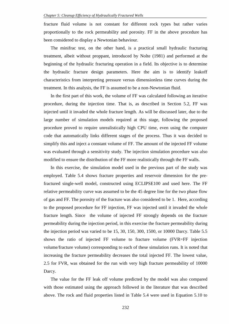
Chapter 5: Cleanup Efficiency of Hydraulically Fractured Wells
232
fracture fluid volume is not constant for different rock types but rather varies
proportionally to the rock permeability and porosity. FF in the above procedure has
been considered to display a Newtonian behaviour.
The minifrac test, on the other hand, is a practical small hydraulic fracturing
treatment, albeit without proppant, introduced by Nolte (1981) and performed at the
beginning of the hydraulic fracturing operation in a field. Its objective is to determine
the hydraulic fracture design parameters. Here the aim is to identify leakoff
characteristics from interpreting pressure versus dimensionless time curves during the
treatment. In this analysis, the FF is assumed to be a non-Newtonian fluid.
In the first part of this work, the volume of FF was calculated following an iterative
procedure, during the injection time. That is, as described in Section 5.2, FF was
injected until it invaded the whole fracture length. As will be discussed later, due to the
large number of simulation models required at this stage, following the proposed
procedure proved to require unrealistically high CPU time, even using the computer
code that automatically links different stages of the process. Thus it was decided to
simplify this and inject a constant volume of FF. The amount of the injected FF volume
was evaluated through a sensitivity study. The injection simulation procedure was also
modified to ensure the distribution of the FF more realistically through the FF walls.
In this exercise, the simulation model used in the previous part of the study was
employed. Table 5.4 shows fracture properties and reservoir dimension for the pre-
fractured single-well model, constructed using ECLIPSE100 and used here. The FF
relative permeability curve was assumed to be the 45 degree line for the two phase flow
of gas and FF. The porosity of the fracture was also considered to be 1. Here, according
to the proposed procedure for FF injection, FF was injected until it invaded the whole
fracture length. Since the volume of injected FF strongly depends on the fracture
permeability during the injection period, in this exercise the fracture permeability during
the injection period was varied to be 15, 30, 150, 300, 1500, or 10000 Darcy. Table 5.5
shows the ratio of injected FF volume to fracture volume (FVR=FF injection
volume/fracture volume) corresponding to each of these simulation runs. It is noted that
increasing the fracture permeability decreases the total injected FF. The lowest value,
2.5 for FVR, was obtained for the run with very high fracture permeability of 10000
Darcy.
The value for the FF leak off volume predicted by the model was also compared
with those estimated using the approach followed in the literature that was described
above. The rock and fluid properties listed in Table 5.4 were used in Equation 5.10 to

Chapter 5: Cleanup Efficiency of Hydraulically Fractured Wells
233
calculate the fluid leakoff coefficient as 0.012 ft/min0.5
. It should be noted that the
differential pressure across the core was assumed to be 1000 psi (Howard and Fast,
1970). Then, using Equations 5.5, 5.6 and 5.2; FVR was estimated to be 22. This value
is close to the value obtained from the simulation with the fracture permeability of
around 150 D, Table 5.5 and Figure 5.26. It should be noted that the FF viscosity used
in such calculations is generally greater than 0.5 cp. In a sensitivity study, the FF
viscosity was increased from 0.5 to 5, 50 or 500, giving FVR of 3.1, 1.3 or 1.0,
respectively. These results indicate that the FF injection volume is very sensitive to the
filtrated FF viscosity.
Based on the above investigation, it was decided to inject a constant volume of FF
that invades all the fracture cells instantly, i.e. they are fully saturated with FF at the
start of the injection simulation period and the additional injected FF volume is
distributed across all the cells adjacent to the fracture cells. In this procedure, the FF
saturation distribution within the matrix, which contributes to the performance of
cleanup to much greater extent than that within fracture, is obtained by the simulator but
that within the fracture is assumed to happen instantly, which is somewhat consistent
with what happens in reality and is reported in the literature. Thus to be able to observe
the impact of pertinent parameters, the author suggested using FVR values of 2 and 5
that correspond to fracture permeabilities of 10000 and 1500 Darcy.
5.4.2 Range and Number Of Investigated Variables
Tables 5.6 and 5.7 show the ranges of variation of pertinent parameters that need to
be investigated in the numerical simulations. There are 16 parameters for both the
injection and the production periods in these two Tables, a total of 32 . Equations 5.11-
5.14 describe the capillary pressure and relative permeability curves for data of these
Tables.
5.00075.0 KIFT
Pd (5.11)
o Threshold pressure Pd (bar)
o Interfacial tension IFT (dyne/cm)
o Matrix permeability (K (mD))
Swr
SwrSw
Pc
Pd
1
(5.12)
nw
rwSgrSwr
SwrSwwKk
1max (5.13)

Chapter 5: Cleanup Efficiency of Hydraulically Fractured Wells
234
ng
rgSgrSwr
SgrSggKk
1max (5.14)
To conduct these simulations, the author looked at a number of designs and used 2-
level full factorial design. To obtain a response surface for a system with “p” parameters
using the full factorial design of the second order, the number of required experiments is
2p.
To cover the range of variation of all 32 parameters, based on full factorial design,
4.3E9 simulations are required, for which, assuming it takes only one second to
complete each simulation, it would take 136 years to complete these simulations, for
one of the two FVR values. As will be described below, each simulation will take
around 15 second, which gives an unrealistic simulation time of 2040 years. Therefore,
it was suggested to approach this in a stepwise manner. That is, initially, simulations
using post treatment input parameters (Table 5.7) for both injection and production
periods are conducted. This will reduce the number of simulations to 65536 for each of
the two FVR values.
Computer Code
It was mentioned before that a computer code was developed which automatically
linked different stages of the simulation process.
In this computer code, initially, the experimental design matrix is read, and then for
each case, kr and Pc curves are generated as include-files. The program also creates
another three include-files for porosity, permeability (matrix and fracture) and bottom
hole pressure. It should be noted that these include-files are used for simulation of both
injection and production periods. The initial conditions for the production period
(pressure and saturation distribution) are those read using the restart files at the last time
step of the injection period. To evaluate the FF cleanup efficiency for these cases a
100% cleanup efficiency case is also required to be simulated. This is performed by
running a case with the injected FF volume set to zero. After running these cases using
Eclipse, total gas and total FF production from summary files are read for three
production times, 10, 30 and 365 days.
After performing one simulation with the above procedure it was noted that each
simulation run takes about 15 seconds to complete. The estimated CPU time for the
65536 simulation runs, required to investigate the variation of 16 parameters of the
production period (considering full factorial design of second order), is 23 days for each
fracture volume. As mentioned above, if the previous procedure (FF injected until the

Chapter 5: Cleanup Efficiency of Hydraulically Fractured Wells
235
whole fracture is filled with FF) is followed, the required CPU time will be significantly
more.
Response Surface Method (RSM)
The RSM is a useful tool to analyse sensitivity study. As discussed in chapter 3, the
response surface method (RSM) is a combination of statistical and mathematical
methods to find an appropriate relationship between the response y and independent
variables x1, x2, x3... xn. It fits a polynomial function to the response of the y. The
polynomial function f is called the response surface model. This model can be a linear
(with or without interaction term) or quadratic model defined by Equations 5.11 and
5.12, respectively.
n
i
n
ij
jiji
n
k
nk xxaaxaay11
0 (Linear response model) (5.11)
n
i
n
ij
jiji
n
k
kk
n
k
nk xxaaxaxaay11
2
1
0 (Quadratic response model) (5.12)
The coefficient of the above function is determined by least square method.
In this research work, the author used only the linear response model to describe the
dependency of gas production loss (GPL) on parameters affecting the cleanup efficiency
of a HFW. This is mainly due to the fact that using a full factorial design, which covers
a more representative range of variation of parameters, with quadratic terms requires a
significantly higher number of simulations. Here, based on the 3-level full factorial
experiment design, the number of the required simulations is 43046721, which requires
a significant CPU time of 491 years to be completed if each run takes 5 second as
described above. There are other experiment designs, requiring lower number of
simulations e.g. Box-Behken and Central Composite Design (CCD), which are beyond
of the scope of this work.
5.4.3 Results
Over 130000 runs were performed for two FF injection volumes. As mentioned
earlier, the simulation procedure was automatically run by the computer code and
output data were written into output files. These files were used to calculate GPL for
each run at three different time steps, after 10, 30 and 365 production days. The linear
response surface models with (referred to hereafter as LRSM) and without (referred to
hereafter as ILRSM) the interaction terms were used to relate the response (GPL) to the

Chapter 5: Cleanup Efficiency of Hydraulically Fractured Wells
236
variation of the sixteen parameters. The least square method was used to estimate the
regression coefficients in the models. Here, the author used the statistical tools of
MATLAB software for this multiple-regression exercise.
As expected, the ILRSM gives a better prediction of GPL because of having more
tuning parameters. That is, for the case of using LRSM there are the intercept and 16
coefficients of the main parameters whilst ILRSM has 120 additional interaction
coefficients. Accordingly, the corresponding multiple determination coefficient (R2) for
ILRSM, 0.94, was higher than that for LRSM, 0.9.
Figure 5.27 shows the percentage of the cumulative frequency of the cases with
FVR=2 versus the GPL% at three different production times. The results indicate that as
production of gas and FF continues the number of the cases with severe production loss
decreases. For example, 85% of the cases have GPL of more than 20% after 10
production days, while this is reduced to 70% of the cases and 25% for 30 and 365 days
of production.
The coefficients of the LRSM of GPLs with and without interaction parameters when
FVR=2 are shown in Tables 5.8 and 5.9.
The magnitude and significance of impacts of the parameters can be evaluated by
comparing the corresponding coefficients, i.e. the parameter with higher absolute value
of the coefficient has a higher impact on GPL. As illustrated in Table 5.9, the intercept
has the highest value for all the time steps studied here. The absolute value of the
coefficient of the fracture permeability is higher than the corresponding values for other
parameters, highlighting the fact that GPL is significantly affected by this parameter.
The impact of Sgrf on the GPL is negligible compared to other parameters.
The relative importance of each parameter for different scenarios can be more easily
compared with those under different prevailing conditions (e.g. different production
time intervals or FFV) if they are scaled by dividing them by the coefficient which has
the highest absolute value in the fitted response model. It should be noted that as gas
and FF is produced, the GPL decreases. Therefore, the importance of the parameters
affecting GPL varies with time. For early time of production, GPL is high for the most
cases, which imposes the high value for the intercept. However, as the production time
increases, GPL and consequently the absolute value of the intercept of the response
surface model decreases. This can also be confirmed by comparing the intercept values
of LRM for 10, 30 and 365 days of production, Table 5.8.
Figures 5.28, 5.29 and 5.30 show the scaled coefficients of all parameters affecting
GPL at three different production periods. It is noted that all the scaled values of the

Chapter 5: Cleanup Efficiency of Hydraulically Fractured Wells
237
primary coefficients, after 10 days of production, are less than 0.5, Figure 5.28. This
indicates the impact of the primary coefficient are more or less the same because during
this period, a large amount of FF is produced. It is very clear that kf with the scaled
value of -0.39 has the most contribution to the GPL sensitivity. Six other important
parameters, which influence GPL are ngf, Kmaxwf, dp , km, ngm and nwf with the scaled
primary coefficient values of 0.21, -0.19, -0.18, -0.17 , 0.17 and 0.17, respectively. It
seems that GPL decreases as Kmaxwf, dp and km, increase and decreases by an increase in
ngf , nwf and ngm. The scaled values of the primary coefficients of , Kmaxwm,
Kmaxwgf,nwm,Sgrm , Kmaxgm and Sgrf are negligible, i.e. less than or close to 0.1.
As gas and FF produces, GPL decreases and the variation and sensitivity of GPL to
the variables under the study increases. The absolute value of the primary coefficient of
kf increases from 0.37 to -0.49. The observed trend of the scaled values of the primary
coefficients of the parameters after 30 production days is more or less similar to those
after 10 production days as the amount of FF being produced is still significant, Figure
5.29. However the number of the parameters which significantly affect GPL has slightly
increased by 1.
Figure 5.30 shows the number of the parameters, which significantly affect GPL,
after 1 year of gas production, has significantly increased because there is no FF to be
produced after 365 days of production, i.e. the fracture is clean. GPL of the majority of
cases under study were below 30%. The absolute values of the scaled primary
coefficients increases significantly, i.e. the corresponding values for kf and ngf increase
from -0.49 and 0.28 shown in Figure 5.29 to -0.7 and 0.38 in Figure 5.30, respectively.
Figure 5.31, which compares the three different scaled coefficients after 10, 30 and
365 days of production shows that the impact of the parameters is increasing with
continued production of gas and FF. As noted earlier, this is mainly due to the fact that,
as production continues the amount of FF produced with gas decreases, i.e. its adverse
impact on gas production decreases, which in turn exaggerates the impact of parameters
affecting the cleanup.
Figure 5.32 shows a comparison of the corresponding scaled coefficients of the
variables for LRSM and ILRSM fits after 30 and 365 days of production, when
FVR=2.0. The scaled coefficients are almost identical for 30 days of production.
However, after 365 days of production, the scaled coefficients of RSM are significantly
less than those of the ILRSM. The values of the scaled coefficients of the interaction
terms, on the other hand, are small for 10 and 30 days of production but increases
significantly after 365 days of production, Table 5.10. These results suggest that the

Chapter 5: Cleanup Efficiency of Hydraulically Fractured Wells
238
coefficients of the main parameters are controlling the extent of GPL, which was rather
high at low production periods. Furthermore, it can be concluded that no direct
comparison can be made between the coefficients of the main terms of LRSM and
ILRSM after 365 production days.
From Table 5.10, it is noted that amongst the 120 interaction coefficients
(120=p*(p-1)/2 where p, number of parameters is 16), only a few are considerable and
those correspond to 1 year of production. These terms are interaction parameters
between those parameters which affect the GPL significantly such as kf, nwf, Kmaxwf , ngf,
ngm, dp, IFT, , km.
The procedure explained above for analysing the results of simulations with FVR=2
was followed for the output data of the fracture models, with FVR=5. Figure 5.33
compares scaled coefficients for these two FVF values at two different time intervals. It
is noted that the observed trends are more or less similar. The fracture permeability has
the most significant impact on GPL and the sequences of the importance of the other
parameters are somewhat similar. However, the relative importance of the pertinent
parameters when FVR=5 are less than those for FVR=2, especially at higher production
periods. This is mainly due to the increased required time for cleaning the fracture as FF
injection volume increases. As discussed earlier, GPL is a function of time. An increase
in the FF injection volume increases GPL and delays the fracture clean up. This
dampens the relative importance of the parameters. It is also noted that the relative
magnitude of scaled coefficients with higher FVR of 5 at 30 days of production was
similar to that with lower FVR of 2 at 10 days of production, Figure 5.34.
As discussed earlier, increasing the FF volume significantly increases the percentage
of the cases with severe FF damage as shown in Figure 5.35. It is interesting to point out
that the curve of the cases with FVR=2 at 10 production days overlap that of the cases
with FVR=5 at 30 production days, i.e. the GPL function for these two scenarios are
similar.
5.5 SUMMARY AND CONCLUSIONS
This study aimed to evaluate the impact of pertinent parameters on the clean-up
efficiency of a hydraulically (gas or gas-condensate) fractured well. In the first part, a
series of numerical simulations were conducted using ECLIPSE 300 and ECLIPSE100.
The general conclusion is that accurate modeling of FF invasion into the fracture and
matrix is crucial. The main itemized conclusions of the first section are:

Chapter 5: Cleanup Efficiency of Hydraulically Fractured Wells
239
1. A model was created using ECLIPSE100, which reproduced the results of the
published paper by Holditch (1979), thereby demonstrating the integrity of the proposed
approach.
2. The presence of fracture fluid (FF) in the damage zone influences gas recovery by
reducing the gas relative permeability. It can increase gas production loss (GPL)
significantly, if FF invasion can be simulated more realistically, as was performed here
by allowing the FF to invade all fracture blocks. This supports experimental work
conducted by Bennion (2001). However, it does not agree with the numerical
simulations conducted by several other investigators (Holditch 1979, Adegbola 2002,
Gdanski et al. 2005).
3. The results also demonstrate that the combined effect of absolute permeability
and effective gas relative permeability reduction in the matrix invaded zone is more
pronounced for most of considered cases studied here, even for the cases with moderate
to high fracture permeability reduction. This is in contrast with the previous numerical
models, showing that fracture face damage is the important issue if it caused severe
permeability reduction in the matrix invaded zone.
4. FF recovery is higher if it is degraded with a reduced viscosity, i.e., higher
mobility for the production period.
5. The fracture conductivity reduction is the main factor in GPL, when matrix
capillary pressure is zero. Matrix capillary pressure increases the extent of FF invasion
into the matrix. This reduces the saturation of FF in the fracture, thus reducing the
impact of fracture on cleanup efficiency.
6. Damage permeability reduction in the range of 90% and 99% can significantly
increase GPL when matrix capillary pressure is considered.
7. The initial water saturation (Swi) decreased GPL. This is due to a decrease in the
capillary pressure driving force between matrix and fracture, which in turn reduces the
FF invasion into the matrix. It should be noted that this conclusion is based on the 100%
cleanup case with Swi, where the gas production has already dropped significantly due to
the presence of Swi.
8. The effect of a change in the matrix capillary pressure of the damaged zone is
negligible unless unrealistically low pressure drawdown is assumed. This is in line with
the findings in the literature (e.g., Holditch (1979) & Gdanski (2005)).
9. FF recovery was improved in the presence of condensate, which resulted in a
decrease in the adverse effect of FF, giving lower GPL. It should be noted that this

Chapter 5: Cleanup Efficiency of Hydraulically Fractured Wells
240
conclusion is based on a 100% cleanup case with fixed bottom hole pressure below dew
point, where the gas production has already dropped due to condensate dropout.
10. Improving the relative permeability of an oil based FF compared to a water
based FF decreased GPL.
11. The hysteresis had a negligible effect on GPL.
In the second part of this study, a new methodology was developed to further
investigate the impact of the pertinent parameters on the clean up efficiency. A 2-level
full factorial statistical experimental design was used to sample a reasonably wide range
of variation of pertinent parameters, covering many practical cases. The variation of a
total of 16 parameters describing the matrix and fracture relative permeability of gas
and FF, matrix capillary pressure were studied for two separate FF volume values
(FVR=2 and 5). Due to the large number of simulations required for this purpose, a
computer code was developed using MATLAB mathematical package, which linked
automatically different stages of the simulations conducted using ECLIPSE100. Over
130000 simulation runs were performed for many different prevailing conditions. The
gas production loss (GPL) compared to the 100% cleanup case was also calculated
automatically as an output data for each run at different production periods after the FF
injection. The linear repose surface without (LRSM) and with interaction parameters
(ILRSM) models were used to relate the response (GPL) to the variation of the sixteen
parameters. The least square method was used to estimate the regression coefficients in
the models.
The analysis of the data for the fracture models with FVR=2 demonstrated that:
12. As FF and gas production continues, the number of the cases with severe gas
production loss decreases but the relative importance of the pertinent parameters
increases.
13. GPL is significantly affected by fracture conductivity.
14. The impact of residual gas saturation in the fracture and gas end point of a Corey
type relative permeability curve on the GPL is negligible.
15. The other important parameters, which influence GPL are the FF exponent and
end point of the Corey type relative permeability curve in the fracture, the gas exponent
of the Corey type relative permeability curve in the fracture and matrix, differential
pressure across the reservoir, interfacial tension, the pore size distribution index, matrix
permeability, the end points of the Corey type relative permeability curve in the matrix,
residual gas saturation in the matrix and porosity.

Chapter 5: Cleanup Efficiency of Hydraulically Fractured Wells
241
16. The presence of interaction parameters in the linear response surface fit resulted
in better prediction because of having more tuning terms, i.e. interaction coefficients.
17. Amongst 120 interaction terms, only a few terms are considerable and they
correspond to 1 year of production.
18. The scaled coefficients of the main terms of LRSM and those of ILRSM for
GPL after 10 and 30 days of production, where GPL was large, were similar. It seems
that the coefficients of the main terms were mainly affected the extent of GPL.
The analysis of the data for the fracture models with FVR=5 supports the main
conclusion of those with FVR=2. However, there are some differences as follows:
19. Increasing the FF volume from 2 to 5 significantly increases the percentage of
the cases with severe FF damage.
20. An increase in the FF injection volume increases GPL and delays the fracture
clean up.
21. The relative importance of pertinent parameters when FVR=5 are less than those
when FVR=2, especially at higher production periods.

Chapter 5: Cleanup Efficiency of Hydraulically Fractured Wells
242
References
Adegbola K. and Boney C., 20-21 Feb 2002: Effect of Fracture Face Damage on Well
Productivity, SPE 73759.
Barati R., Hutchins R.D., Friedel T., Ayoub J.A., Dessinges M. and England K.W. ,
13–15 February 2008: Impact of Yield Stress and Fracture-Face Damage on Production
Using a Three-Phase, 2D Model, SPE 111457.
Bennion D. B., Thomas F. B. and Ma T., 12-15 March 2001: Recent Advances in
Laboratory Test Protocols to Evaluate Optimum Drilling, Completion and Stimulation
Practices for Low Permeability Gas Reservoirs, SPE 60324.
Cooke, C.E., October 1975: Effect of fracturing fluids on fracture conductivity, JPT, pp.
1273-83, Trans., AIME, 259.
Cooke, C.E., Sep 1973: Conductivity of Fracture Proppants in Multiple Layers, SPE
4117, JPT.
Gdanski, R., Weaver, J., Slabaugh, B., Walters H. and Parker M., May 2005: Fracture
Face Damage-It Matters, SPE 94649.
Geertsma J. and de Klerk F., 1969: A rapid method of predicting width and extent of
hydraulically induced fractures. J Pet Tech 1969; 21:1571–81 [SPE 2458].
Ghahri P., Jamiolahmady M. and Sohrabi M. , 27–29 May 2009: Investigation of
Cleanup Efficiency of Hydraulically Fractured Wells in Gas Condensate Reservoirs,
SPE 121916, SPE European Formation Damage Conference held in Scheveningen The
Netherlands.
Holditch S. A., Dec 1979: Factors Affecting Water Blocking and Gas Flow from
Hydraulically Fractured Gas Wells, JPT 1515-1524.
Howard G.C. and Fast, C.R., 1957: Optimum Fluid Characteristics for Fracture
Extension, Drilling and Production Prac., API 24, 261–270.
Khristianovic S.A. and Zheltov Y.P., 1955: Formation of vertical fractures by means of
highly viscous liquid. In: Proceedings of the fourth world petroleum congress, Rome,
pp. 579–86.
Jamiolahmady M., Danesh A, Tehrani D.H. and Mehran Sohrabi, 2006: Variations of
Gas-Condensate Relative Permeability with Production Rate at Near Wellbore
Conditions, A general Correlation, SPE Reservoir Engineering and Evaluation Journal,
9 (6), pp.688-697.
Naar J. and Henderson J.H., June 1961: An Imbibition Model-Its Application to Flow
Behaviour and Prediction of Oil Recovery, SPE1550-G.

Chapter 5: Cleanup Efficiency of Hydraulically Fractured Wells
243
Friedel T., Mtchedlishvili G., Behr A., Voigt H-D. and Hafner F. , 30 May-1 June
2007: Comparative Analysis of Damage Mechanism in Fractured Gas Wells, SPE
107662.
Nolte K.G. and Smith M.B., 1981: Interpretation of fracturing pressures, J Pet Tech
1981; (September):1767–75.
Nordren R.P., 1972: Propagation of a vertical hydraulic fracture, SPE J 1972;
12(8):306–14 [SPE 7834].
Perkins, T.K. and Kern L.R., 1961: Width of Hydraulic Fractures, paper SPE 89,
Journal of Petroleum Technology (Sep 1961) 13, No. 9, 937-949.
Voneiff G.W., Robinson B.M. and Holditch S.A., Nov 1996: The Effects of Unbroken
Fracture Fluid on Gaswell Performance, SPE-26664.
Wang J.Y., Holditch S.A. and MacVay D., Jan 2009: Modelling Fracture Fluid Cleanup
in Tight Gas Wells, SPE-119624.

Chapter 5: Cleanup Efficiency of Hydraulically Fractured Wells
244
Table 5.1: The prevailing conditions and loss of gas production due to the effect of Sffm
and kfd for a selected number of scenarios simulating the effect of hysteresis on the
cleanup efficiency of the hydraulically fractured single well model. Index hysteresis Time(days) R2(Sffm&kfd)% R3(Sffm)% R4(kfd)%
Rh1a (Pc, krg)dra&imb 300 - -
Rh2a (Pc, krg)dra&imb 300 70 30 40
Rh3a (Pc, krg)dra&imb 300 30 30
Rh1b (Pc, krg)dr 300 - - -
Rh2b (Pc, krg)dr 300 68 30 38
Rh3b (Pc, krg)dr 300 30 30
Rh1c (Pc)dra, (krg)dra&imb 300 - - -
Rh2c (Pc)dra, (krg)dra&imb 300 69 30 39
Rh3c (Pc)dra, (krg)dra&imb 300 - 30 30
Rh1d (Pc)dra, (krg)dra&imb 400 - - -
Rh2d (Pc)dra, (krg)dra&imb 400 65 30 35
Rh3d (Pc)dra, (krg)dra&imb 400 - 30 30
Rh1e (Pc)dra, (krg)imb 300 - - -
Rh2e (Pc)dra, (krg)imb 300 72 30 42
Rh3e (Pc)dra, (krg)imb 300 - 30 30
Rh1f (Pc)dra, (krg)imb 400
Rh2f (Pc)dra, (krg)imb 400 68 29 39
Rh3f (Pc)dra, (krg)imb 400 29 29
Table 5.2: Reservoir and fracture Properties, Holditch well model study (1979). Matrix Porosity 0.08
Matrix Permeability 0.1
Fracture Length 660 ft
Fracture width 0.006 m
Fracture Porosity 0.20
Table 5.3: Reproduction of Holditch Damage Effect- a) the original work–Holditch
(1979) b) Reproduced data.
(a) (b)
Table 5.4: The basic input data for the cases A and B.
Xf(m) wf(m) Xres(m) Yres(m) Zres(m) Vf(m3) Kf(D)* km(mD)* (%)* (cp)*
400 0.004 2000 2000 40 64 15 0.18 17 0.5
* For both injection and production period
Swi=0, Pcm=0
(JDamage/JUndamage)× 100
Cf (md-ft) 100 10 1 0.1
100 100 99.1 93.1 61.0
500 100 99.0 91.5 55.8
4000 100 98.7 90.5 53.8
(JDamage/JUndamage)× 100
Cf (md-ft) 100 10 1 0.1
100 100 99.2 93 61.6
500 100 99 91.3 54.2
4000 100 98.2 90.2 50.8

Chapter 5: Cleanup Efficiency of Hydraulically Fractured Wells
245
Table 5.5: The ratio of injected FF per fracture volume for different fracture
permeability used in this study. kinj(D) Vinj(m3) Vinj/Vf
15 3096 96.7
30 1887 59.0
150 615 19.2
300 361 11.3
1500 149 4.7
3000 112 3.5
10000 80 2.5

Chapter 5: Cleanup Efficiency of Hydraulically Fractured Wells
246
Table 5.6: Uncertain parameters before treatment.
Parameter Min Max
Fracture Conductivity Kf (D) 1 30
Pressure Drawdown p (bar) 30 250
Matrix Permeability Km 1 D 0.1 mD
Matrix capillary pressure curve (Pc) Pore size index 1 3
Matrix capillary pressure curve (Pc) Threshold pressure Eq. (5.11) Eq.(5.11)
Matrix capillary pressure curve (Pc) Interfacial Tension (mNm/m) 10 50
Porosity 0.05 0.15
Matrix krg curve Sgr 0.25 0.6
Matrix krw curve Swr 0.1 0.3
Matrix krg curve ng 2 6
Matrix krw curve nw 1.5 6
Matrix krg curve Kmaxg(end point) 0.7 1.0
Matrix krw curve Kmaxw(end point) 0.1 0.5
Fracture krg curve Sgr 0.1 0.3
Fracture krw curve Swr 0.1 0.3
Fracture krg curve ng 2 6
Fracture krw curve nw 2 6
Fracture krg curve Kmaxg(end point) 0.9 1
Fracture krw curve Kmaxw(end point) 0.15 0.55
Table 5.7: Uncertain parameters after treatment. Parameter Min Max
Fracture Conductivity Kf (D) 1 30
Pressure Drawdown p (bar) 30 250
Matrix Permeability Km 1 D 0.1 mD
Matrix capillary pressure curve (Pc) Pore size index 1 4
Matrix capillary pressure curve (Pc) Threshold pressure Eq. (5.11) Eq. (5.11)
Matrix capillary pressure curve (Pc) Interfacial Tension
(mNm/m)
2 50
Porosity 0.05 0.15
Matrix krg curve Sgr 0.1 0.6
Matrix krw curve Swr 0.1 0.1
Matrix krg curve ng 1.5 5
Matrix krw curve nw 1.2 4
Matrix krg curve Kmaxg(end point) 0.5 1.0
Matrix krw curve Kmaxw(end point) 0.05 0.6
Fracture krg curve Sgr 0.1 0.3
Fracture krw curve Swr 0.1 0.1
Fracture krg curve ng 1.5 5
Fracture krw curve nw 1.2 4
Fracture krg curve Kmaxg(end point) 0.5 1.0
Fracture krw curve Kmaxw(end point) 0.1 0.75

Chapter 5: Cleanup Efficiency of Hydraulically Fractured Wells
247
Table 5.8: The coefficients estimated for the linear response model of GPL by least
square method Production days
Parameters
After 365 After 30 After 10
Intercept 22.1 60.1 76.6
Kf (x1) -15.3 -29.4 -28.7
dp (x2) -7.4 -13.9 -14.0
km (x3) -5.3 -12.9 -13.3
Lam ( )(x4) 5.3 9.6 8.3
IFT(x5) -5.5 -10.0 -8.9
Porosity ( )(x6) -3.0 -5.9 -5.9
Sgrm (x7) 3.2 6.7 7.3
ngm (x8) 7.4 13.8 13.3
nwm (x9) 3.6 4.6 3.9
Kmaxgm (x10) -1.0 -2.2 -2.5
Kmaxwm (x11) -4.6 -7.4 -6.6
Sgrf (x12) -0.4 -0.3 -0.2
ngf (x13) 8.5 15.9 16.5
nwf (x14) 12.2 16.0 13.6
Kmaxgf (x15) -4.0 -5.6 -5.2
Kmaxwf (x16) -9.0 -15.5 -15.1
Table 5.9: The coefficients of the main effects estimated for the linear interaction
response model of GPL by least square method. Production days
Parameters
After 365 After 30 After 10
Intercept 22.6 68.5 83.1
Kf (x1) -20.6 -39.3 -32.7
dp (x2) -7.2 -9.6 -6.5
km (x3) -6.1 -11.6 -7.6
Lam ( )(x4) 10.8 10.1 5.0
IFT(x5) -15.1 -23.4 -16.9
Porosity ( )(x6) -4.2 -7.0 -5.1
Sgrm (x7) 5.3 8.5 7.6
ngm (x8) 13.3 17.8 12.7
nwm (x9) 0.1 -2.1 -3.0
Kmaxgm (x10) -2.2 -3.4 -3.4
Kmaxwm (x11) -4.5 -5.2 -2.6
Sgrf (x12) -0.8 -0.6 -0.3
ngf (x13) 14.1 16.9 12.7
nwf (x14) 17.5 2.8 -6.1
Kmaxgf (x15) -4.8 -5.0 -3.9
Kmaxwf (x16) -12.6 -18.6 -13.6

Chapter 5: Cleanup Efficiency of Hydraulically Fractured Wells
248
Table 5.10: The scaled coefficients for interaction terms (IRSM) Production
days
Scaled Coefficients
After
365
After 30 After 10
x1x2 0.24 0.02 -0.06
x1x3 0.41 0.13 0.02
x1x4 -0.29 0.01 0.07
x1x5 0.46 0.04 -0.07
x1x6 0.10 0.02 -0.01
x1x7 0.00 0.01 0.03
x1x8 -0.22 0.00 0.07
x1x9 -0.10 -0.01 0.01
x1x10 0.05 0.01 0.00
x1x11 0.13 0.02 -0.02
x1x12 0.02 0.00 0.00
x1x13 -0.37 -0.04 0.03
x1x14 -0.46 0.04 0.11
x1x15 0.13 0.00 -0.03
x1x16 0.36 0.04 -0.06
x2x3 -0.08 -0.11 -0.14
x2x4 -0.23 -0.14 -0.10
x2x5 0.24 0.14 0.10
x2x6 0.11 0.03 0.01
x2x7 -0.20 -0.07 -0.03
x2x8 -0.27 -0.07 -0.01
x2x9 -0.04 0.01 0.01
x2x10 0.03 0.00 0.00
x2x11 0.14 0.03 0.00
x2x12 0.00 0.00 0.00
x2x13 -0.13 -0.02 0.01
x2x14 -0.05 0.07 0.08
x2x15 0.03 -0.01 -0.02
x2x16 0.18 0.00 -0.05
x3x4 -0.24 -0.08 -0.03
x3x5 0.23 0.05 -0.01
x3x6 0.08 0.01 -0.01
x3x7 -0.19 -0.05 -0.01
x3x8 -0.22 -0.03 0.01
x3x9 0.01 0.01 0.01
x3x10 0.03 0.00 -0.01
x3x11 0.08 0.01 0.00
x3x12 0.00 0.00 0.00
x3x13 -0.14 -0.04 -0.01
x3x14 0.01 0.09 0.10
x3x15 0.00 -0.02 -0.02
x3x16 0.09 0.00 -0.04
x4x5 0.06 0.17 0.14
x4x6 -0.02 0.02 0.02
x4x7 0.05 0.02 0.01
x4x8 0.07 -0.02 -0.04
x4x9 0.02 -0.03 -0.03
x4x10 -0.01 0.00 0.01
x4x11 -0.01 0.04 0.04
x4x12 0.00 0.00 0.00
x4x13 0.12 0.02 0.00
x4x14 0.09 -0.01 -0.02
x4x15 -0.03 0.00 0.00
x4x16 -0.06 -0.02 0.00
x5x6 -0.02 -0.03 -0.04
x5x7 0.08 0.03 0.02
x5x8 0.03 0.07 0.08
x5x9 0.02 0.03 0.03
x5x10 0.00 -0.01 -0.01
x5x11 -0.04 -0.06 -0.05
x5x12 0.00 0.00 0.00

Chapter 5: Cleanup Efficiency of Hydraulically Fractured Wells
249
x5x13 -0.21 -0.07 -0.03
x5x14 -0.15 0.00 0.03
x5x15 0.04 0.01 0.00
x5x16 0.11 0.04 0.01
x6x7 -0.05 0.00 0.00
x6x8 -0.10 -0.01 0.01
x6x9 -0.05 -0.01 0.00
x6x10 0.01 0.00 0.00
x6x11 0.06 0.01 0.00
x6x12 0.00 0.00 0.00
x6x13 -0.03 -0.01 0.00
x6x14 0.02 0.03 0.03
x6x15 0.00 -0.01 -0.01
x6x16 0.01 -0.01 -0.02
x7x8 0.13 -0.01 -0.05
x7x9 0.09 0.03 0.03
x7x10 0.03 0.03 0.03
x7x11 -0.10 -0.04 -0.03
x7x12 0.01 0.00 0.00
x7x13 0.04 0.00 -0.01
x7x14 -0.04 -0.04 -0.04
x7x15 0.01 0.01 0.01
x7x16 -0.02 0.01 0.03
x8x9 0.21 0.09 0.06
x8x10 -0.02 0.00 0.01
x8x11 -0.20 -0.11 -0.09
x8x12 0.00 0.00 0.00
x8x13 0.07 0.00 -0.03
x8x14 0.05 -0.04 -0.05
x8x15 -0.01 0.01 0.02
x8x16 -0.05 0.01 0.03
x9x10 -0.01 0.00 0.00
x9x11 0.04 0.05 0.04
x9x12 0.00 0.00 0.00
x9x13 0.04 0.00 -0.01
x9x14 0.15 0.05 0.03
x9x15 -0.04 -0.01 -0.01
x9x16 -0.01 0.00 0.00
x10x11 0.01 0.00 0.00
x10x12 0.00 0.00 0.00
x10x13 -0.02 -0.01 0.00
x10x14 0.00 0.01 0.01
x10x15 0.00 0.00 0.00
x10x16 0.02 0.00 0.00
x11x12 0.01 0.00 0.00
x11x13 -0.05 0.00 0.02
x11x14 -0.12 -0.03 -0.01
x11x15 0.03 0.01 0.00
x11x16 0.04 0.00 -0.01
x12x13 0.00 0.00 0.00
x12x14 -0.04 -0.01 -0.01
x12x15 0.01 0.00 0.00
x12x16 0.04 0.01 0.00
x13x14 0.46 0.18 0.12
x13x15 0.02 0.04 0.04
x13x16 -0.29 -0.09 -0.05
x14x15 -0.21 -0.04 -0.01
x14x16 -0.18 0.08 0.11
x15x16 0.10 0.00 -0.01

Chapter 5: Cleanup Efficiency of Hydraulically Fractured Wells
250
Pc Curves
0
50
100
150
200
250
300
350
400
450
500
0 0.2 0.4 0.6 0.8 1Sw
Pc(
Psi
a)
Drainage
Imbibition
Figure 5.1: Capillary pressure curves used here.
0.00
0.20
0.40
0.60
0.80
1.00
0 0.05 0.1 0.15 0.2 0.25 0.3 0.35 0.4
Condensate or Fracturing Fluid Saturation
Rel
ativ
e P
erm
eabil
ity (
kr)
krg-Imbibition
krg-Drainage
RC1b, k=0.18 mD, Sgr=0.65, b=1.06E12 m-1
Figure 5.2: Relative permeability curves used for the effect of hytestersis on cleanup
efficiency.
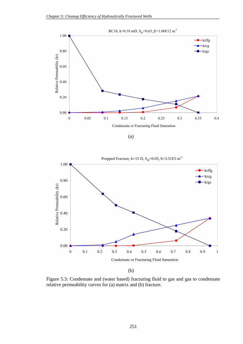
Chapter 5: Cleanup Efficiency of Hydraulically Fractured Wells
251
0.00
0.20
0.40
0.60
0.80
1.00
0 0.05 0.1 0.15 0.2 0.25 0.3 0.35 0.4
Condensate or Fracturing Fluid Saturation
Rel
ativ
e P
erm
eab
ilit
y (
kr)
krffg
krcg
krgc
RC1b, k=0.18 mD, Sgr=0.65, =1.06E12 m-1
(a)
0.00
0.20
0.40
0.60
0.80
1.00
0 0.1 0.2 0.3 0.4 0.5 0.6 0.7 0.8 0.9 1
Condensate or Fracturing Fluid Saturation
Rel
ativ
e P
erm
eab
ilit
y (
kr)
krffg
krcg
krgc
Propped Fracture, k=15 D, Sgr=0.05, b=3.51E5 m-1
(b)
Figure 5.3: Condensate and (water based) fracturing fluid to gas and gas to condensate
relative permeability curves for (a) matrix and (b) fracture.

Chapter 5: Cleanup Efficiency of Hydraulically Fractured Wells
252
FFvP=1, 10 cp-Pcm=0
6
66
15
45
4
52
7
40
0
10
20
30
40
50
60
70
80
90
100
R1(No-kfd&Sffm) R2(kfd&Sffm) R3(Sffm) R4(kfd)
GP
L C
om
par
ed t
o 1
00
% C
lean
Pcm=0 FFvP=10 cp
Pcm=0 FFvP=1cp
Figure 5.4: GPL compared to 100% cleanup case for simulation runs indexed R1-R4
without Pcm at two different FFvPs.
FFvP=1 cp-Pcm=0
58
72
52 52
0
10
20
30
40
50
60
70
80
90
100
,90%-Pcm=0 ,99%-Pcm=0
GP
L%
Co
mp
ared
to
10
0%
Cle
an
R5(kfd&Sffm+kmd)
R2(kfd&Sffm)
Figure 5.5: GPL compared to 100% cleanup for simulation runs indexed R5 (with 90%
and 99% kmd) and R2 (without kmd) both without Pcm.
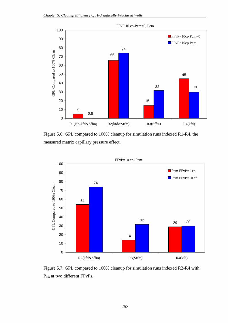
Chapter 5: Cleanup Efficiency of Hydraulically Fractured Wells
253
FFvP 10 cp-Pcm=0, Pcm
5
45
74
66
15
0.6
32 30
0
10
20
30
40
50
60
70
80
90
100
R1(No-kfd&Sffm) R2(kfd&Sffm) R3(Sffm) R4(kfd)
GP
L C
om
par
ed t
o 1
00
% C
lean
FFvP=10cp Pcm=0
FFvP=10cp Pcm
Figure 5.6: GPL compared to 100% cleanup for simulation runs indexed R1-R4, the
measured matrix capillary pressure effect.
FFvP=10 cp- Pcm
54
14
29
74
3230
0
10
20
30
40
50
60
70
80
90
100
R2(kfd&Sffm) R3(Sffm) R4(kfd)
GP
L C
om
par
ed t
o 1
00
% C
lean
Pcm FFvP=1 cp
Pcm FFvP=10 cp
Figure 5.7: GPL compared to 100% cleanup for simulation runs indexed R2-R4 with
Pcm at two different FFvPs.

Chapter 5: Cleanup Efficiency of Hydraulically Fractured Wells
254
FFvP 1 cp-Pcm=0, Pcm
58
7270
85
5254 54
52
0
10
20
30
40
50
60
70
80
90
100
,90%-Pcm=0 ,99%-Pcm=0 ,90%-Pcm ,99%-Pcm
GP
L C
om
par
ed t
o 1
00
% C
lean
R5(kfd&Sffm+kmd)
R2(kfd&Sffm)
Figure 5.8: GPL compared to 100% cleanup for simulation runs indexed R5 (with 90%
and 99% kmd) & R2 (without kmd) both with and without Pcm.
Figure 5.9: Gas production versus time for simulation runs indexed R5 with and
without considering Pcmd.
R5 without Pcmd
R5 with Pcmd

Chapter 5: Cleanup Efficiency of Hydraulically Fractured Wells
255
Figure 5.10: FF production versus time for simulation runs indexed R5 with and
without considering Pcmd.
FFvP=10 cp- Pcm
10
27
17
0
10
20
30
40
50
60
70
80
90
100
R2(kfd&Sffm) R3(Sffm) R4(kfd)
GP
L t
o 1
00
% C
lean
FFvP=1 cp Pcm
Figure 5.11: GPL compared to 100% cleanup for simulation runs indexed R2-R4 with
Pcm corrected for Swi= 17.5%.
R5 with Pcmd
R5 without Pcmd

Chapter 5: Cleanup Efficiency of Hydraulically Fractured Wells
256
FFvP=1 cp-Pcm ,Swi
47
71
27 27
0
10
20
30
40
50
60
70
80
90
100
,90%-Pcm ,99%-Pcm
GP
L%
Co
mp
ared
to
10
0%
Cle
an
R5(kfd&Sffm+kmd)
R2(kfd&Sffm)
Figure 5.12: GPL compared to 100% cleanup for simulation runs indexed R5 (with 90%
and 99% kmd) & R2 (without kmd), both with Pcm and Swi=17.5%.
FFvP=1 cp-Pcm
40
49
9
40
58
18
0
10
20
30
40
50
60
70
80
90
100
R4(kfd) R2(kfd&Sffm) R3(Sffm)
GP
L%
Co
mp
ared
to
10
0%
Cle
an
krnw=1.25
krnw=6
Figure 5.13: GPL compared to 100% cleanup for simulation runs indexed R2-R4 with
Pcm, considering two different FF kr curve.

Chapter 5: Cleanup Efficiency of Hydraulically Fractured Wells
257
0
200
400
600
800
1000
1200
1400
0 5000 10000 15000 20000Times (Day)
GP
R (
MS
CF
/Day
)
Pcmd=0
Pcmd=Pcm
Figure 5.14: Gas production rate vs. times for two cases with Pcmd=Pcm and Pcmd=0.
Figure 5.15: Gas production versus time for simulations R1-R4 with gas and
condensate flow.
R1
R4
R2

Chapter 5: Cleanup Efficiency of Hydraulically Fractured Wells
258
Figure 5.16: FF saturation map after injection of 1227 bbl of FF.
0
0.1
0.2
0.3
0.4
0.5
0.6
0.7
0.8
0.9
1
0 50 100 150 200 250 300 350 400
Time (days)
FF
Blo
ck S
atu
ration insid
e the fra
ctu
re 1
10
FFv(cp)
Figure 5.17: FF saturation in the first fracture grid block versus time.
Fracture Wellbore

Chapter 5: Cleanup Efficiency of Hydraulically Fractured Wells
259
0
5000
10000
15000
20000
25000
0 50 100 150 200 250 300 350 400
Time (days)
GP
R (
MS
CF
/da
ys)
1 cp
10 cp
FFv
Figure 5.18: GPR versus time at two different FF viscosities of 1 and 10 cp.
0
0.1
0.2
0.3
0.4
0.5
0.6
0.7
0.8
0.9
1
0 50 100 150 200 250 300 350 400Time (days)
FF
Sat
ura
tio
n B
lock
in
sid
e F
ract
ure
96
5
kf(D)
Figure 5.19: FF saturation in the first fracture grid block versus time with and without
considering kfd ,FFv=10 cp, both cases with Sffm.
Chapter 5: Cleanup Efficiency of Hydraulically Fractured Wells
260
FFv=1 cp
34
13
21
74
24
50
0
10
20
30
40
50
60
70
80
90
100
R2(kfd&Sffm) R3(Sffm) R4(kfd)
GP
L C
om
par
ed t
o 1
00
% C
lean
kf=5 D
kf=1 D
Figure 5.20: GPL compared to 100% cleanup for simulation runs indexed R2-R4,
FFv=1 cp.
FFv=1 cp
4550
61
23
29
40
21 21 21
0
10
20
30
40
50
60
70
80
90
100
90% 99% 99%
GP
L C
om
par
ed t
o 1
00%
Cle
an
R5(kfd&Sffm+kmd)
R3(Sffm)
R4(kfd)
Figure 5.21: GPL compared to 100% cleanup for simulation runs indexed R3-R5.

Chapter 5: Cleanup Efficiency of Hydraulically Fractured Wells
261
0
0.1
0.2
0.3
0.4
0.5
0.6
0.7
0.8
0.9
1
0 0.2 0.4 0.6 0.8 1
Sg
krf
fg
C-1
C-2
C-3
C-4
krffg
Figure 5.22: FF relative permeability curves versus gas saturation.
0
500
1000
1500
2000
2500
3000
3500
0 50 100 150 200 250 300 350 400
Time (days)
GP
R(M
SC
F/d
ay)
C1C2C3C4
krw
Figure 5.23: The gas production rate versus time with different FF relative permeability
curves inside the fracture.

Chapter 5: Cleanup Efficiency of Hydraulically Fractured Wells
262
0
100
200
300
400
500
600
700
800
900
0 50 100 150 200 250 300 350 400
Time (days)
FF
PT
(MS
CF
)
C1
C2
C3
C4
krw
Figure 5.24: The total FF production versus time for the fractured well model with four
different FF relative permeability curves inside the fracture during production time.
Figure 5.25: Schematic of hydraulic fractured well model
q
i
2q
i
Lost: spurt +leakoff
x
f Average
w(xf)
hf

Chapter 5: Cleanup Efficiency of Hydraulically Fractured Wells
263
0.0
10.0
20.0
30.0
40.0
50.0
60.0
70.0
80.0
90.0
100.0
0 2000 4000 6000 8000 10000
kf (D)
FV
R=
Vff/V
f
HW
FVR=Vff/Vf=2
Fluid Loss Test
Figure 5.26: FF injected volume per fracture volume, FVR, versus fracture
permeability.
0%
10%
20%
30%
40%
50%
60%
70%
80%
90%
100%
0 20 40 60 80 100
GPL%
Cu
mu
lati
ve
Fre
qu
ency
365
30
10
Production days
Figure 5.27: Cumulative frequency of the percentage of the cases studied here for
FVR=2 at different production time versus GPL.

Chapter 5: Cleanup Efficiency of Hydraulically Fractured Wells
264
After 10 production days
dp
lam
IFT
Intercept
Kmaxwf
Kmaxgf
nwf
ngf
Sgrf
Kmaxwm
Kmaxgm
nwm
ngm
Sgrm
porosity
km
kf
-1 -0.5 0 0.5 1
ai/(Intercept)
Figure 5.28: The impact of scaled coefficients (ai/ (Intercept)), LRSM after 10
production days, FVR=2.
After 30 production days
kf
dp
lam
IFT
Kmaxwf
Kmaxgf
nwf
ngf
Sgrf
Kmaxwm
Kmaxgm
nwm
ngm
Sgrm
Porosity
km
Intercept
-1 -0.5 0 0.5 1ai/(Intercept)
Figure 5.29: The impact of scaled coefficients (ai/ (Intercept)), LRSM after 30
production days, FVR=2.

Chapter 5: Cleanup Efficiency of Hydraulically Fractured Wells
265
After 365 production days
dp
lam
IFT
Kmaxwf
Kmaxgf
nwf
ngf
Sgrf
Kmaxwm
Kmaxgm
nwm
ngm
Sgrm
Porosity
Intercept
km
kf
-1 -0.5 0 0.5 1
ai/(Intercept)
Figure 5.30: The impact of scaled coefficients (ai/ (Intercept)), LRSM after 365
production days, FVR=2.
dp
lam
IFT
Kmaxwf
Kmaxgf
nwf
ngf
Sgrf
Kmaxwm
Kmaxgm
nwm
ngm
Sgrm
Porosity
km
kf
Intercept
-1 -0.5 0 0.5 1
ai/(Intercept)
365
30
10
Production days
Linear RSM Model
Figure 5.31: Comparison of the impact of scaled coefficients (ai/ (Intercept)), LRSM
after 10 with 30 and 365 production days, FVR=2.

Chapter 5: Cleanup Efficiency of Hydraulically Fractured Wells
266
Intercept
kf
km
PorositySgrm
ngm
nwm
Kmaxgm
Kmaxwm
Sgrf
ngf
nwf
Kmaxgf
Kmaxwf
IFT
lam
dp
-1 -0.5 0 0.5 1
ai/(Intercept)
365-Interaction
365-Linear
30-Interaction
30-Linear
Production days-RSM
Figure 5.32: Comparison of the impact of scaled coefficients (ai/ (Intercept)) of
LRSM with IRSM after 30 and 365 production days, FVR=2.
Intercept
kf
km
PorositySgrm
ngm
nwm
Kmaxgm
Kmaxwm
Sgrf
ngf
nwf
Kmaxgf
Kmaxwf
IFT
lam
dp
-1 -0.5 0 0.5 1
ai/(Intercept)
365-5
365-2
30-5
30-2
Production days-Vff/Vf
Figure 5.33: Comparison of the impact of scaled coefficients (ai/ (Intercept)), LRSM
after 30 and 365 production days for FVR=2 with that for FVR=5.
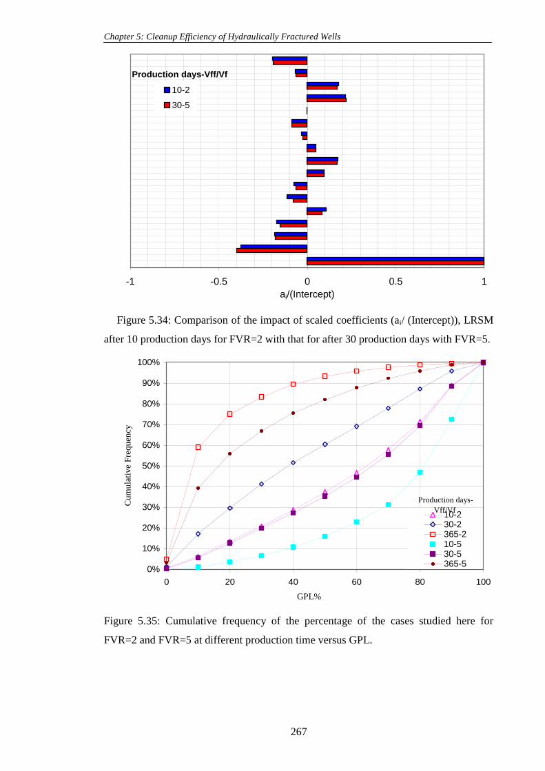
Chapter 5: Cleanup Efficiency of Hydraulically Fractured Wells
267
-1 -0.5 0 0.5 1
ai/(Intercept)
10-2
30-5
Production days-Vff/Vf
Figure 5.34: Comparison of the impact of scaled coefficients (ai/ (Intercept)), LRSM
after 10 production days for FVR=2 with that for after 30 production days with FVR=5.
0%
10%
20%
30%
40%
50%
60%
70%
80%
90%
100%
0 20 40 60 80 100
GPL%
Cu
mu
lati
ve
Fre
qu
ency
10-230-2365-210-530-5365-5
Production days-
Vff/Vf
Figure 5.35: Cumulative frequency of the percentage of the cases studied here for
FVR=2 and FVR=5 at different production time versus GPL.

Chapter 6: Conclusions and Recommendations
268
CONCLUSIONS AND RECOMMENDATIONS
In the last two decades, drilling horizontal (HWs) and deviated (DWs) wells has
become a common practice around the world. An accurate estimation of productivity of
such flow geometries using a numerical simulator is a challenging task. This is mainly
because the 3-D simulation of flow requires a fine grid exercise to capture the abrupt
variation of fluid and flow parameters around the wellbore. This is cumbersome and
impractical for field applications. There are formulations available in the literature for
calculation of productivity of such wells but they are for single-phase flow conditions.
The flow behavior of gas condensate systems, when pressure drops below dew point, is
different from conventional gas oil systems. The phase change and dependency of the
relative permeability to IFT and velocity in the form of coupling and inertia requires a
different approach for these low IFT systems. This study was aimed to propose a
practical methodology, which accounts for the impact of geometrical and flow
parameters, for improved prediction of the performance of HWs and DWs in gas
condensate reservoirs under steady state and pseudo steady state conditions. This was
achieved following a systematic approach as described in Chapters 3 and 4.
Hydraulic fracturing is one of the most important stimulation techniques especially
for tight gas reservoirs. Over the last 60 years, there have been many reports on the poor
performance of some of the hydraulically fractured wells. Poor cleanup efficiency of the
injected fracture fluid (FF) has been considered as one of the factors contributing to the
low productivity of such wells. A number of parametric studies have been conducted
evaluating the impact of a number of pertinent parameters affecting the FF cleanup
efficiency. There are conflicting reports in some of these studies mainly due to the
assumptions made when simulating this process. Therefore to address these issues, the
cleanup efficiency of hydraulically fractured gas and gas-condensate wells was
considered as the other objective of this study. Initially a series of sensitivities were
conducting to clarify some of the uncertainty on the impact of pertinent parameters
affecting the process. Then using statistical methods the effects of key important
parameters, varying over their practical ranges, were extensively investigated by
conducting over 130000 simulations as described in Chapter 5.
The chapter is devoted to present the main conclusions and recommendation for the
future works in these two areas of research.

Chapter 6: Conclusions and Recommendations
269
6.1 CONCLUSIONS
The present research work has three main elements, i) gas condensate flow around
horizontal well, ii) gas condensate flow around deviated wells and iii) cleanup
efficiency of hydraulically fractured wells.
6.1.1 Horizontal Wells (HWs):
This part mainly focuses on proposing practical methods for improved simulation
and well productivity calculation of horizontal wells in gas condensate reservoirs. Here
several single phase and two phase compositional in-house simulators were developed
to model accurately the 3-D complex flow behaviour around a horizontal well in gas
and gas condensate reservoirs under steady state (SS) or pseudo steady state (PSS)
conditions. The integrity of the in-house simulators were confirmed by comparing their
results with those performed using ECLIPSE100 or ECLIPSE300 commercial reservoir
simulators with fine grid under the same privilege conditions. Using the 3-D in-house
simulators a large data bank was generated covering a wide range of variations of
pertinent geometrical and flow parameters. A new formulation and approach was
proposed for calculation of effective wellbore radius of a 1-D open hole radial system
replicating flow around a 3-D system. Series of sensitivity studies were also performed
aimed at investigating the impact of pertinent parameters on the performance of such
wells including identifying the limitations of formulations currently available in the
literature. The major conclusions of this study can be summarized as follows:
1. Horizontal well performance is affected strongly by anisotropy values for
horizontal well length (L) to the reservoir thickness (Z), (L/h) less than
25.
2. Extremely fine grid is required using the commercial simulator
(ECLIPSE) to capture the effect of anisotropy with good accuracy.
3. A combination of increased number of mesh elements and using second
order Lagrange function were required in the finite element based in-
house simulator to obtain accurate results for anisotropic formations.
4. A deviation between the results of the in-house simulator with those
obtained using two well-known equations (Joshi 1991 and Economides
et al. 1996) indicated that these equations may not predict horizontal well
performance properly in anisotropic formations for L/h less than 25.
5. Based on the results of the single phase HW in-house simulator, a
geometric skin was developed using the efficient statistical Response
Chapter 6: Conclusions and Recommendations
270
Surface method. The geometric skin varies with length of horizontal
well, radius of the well, reservoir thickness and anisotropy, the integrity
of the geometric skin formulation was validated by comparing its results
for data points not used in its development. This exercise also included
comparing some of its predictions with those of Joshi (1985) and Borosiv
(1984)‟s semi-analytical equations, with reasonable accuracy. These later
data points were carefully selected to be within the range of applicability
of these equations.
6. The effect of partial penetration (PP) on the well performance of HW and
geometric skin was studied comprehensively. The results indicated that
the partial penetration ratio (horizontal well length (L) to reservoir
dimension in x direction (Xres)) does not have a significant impact on the
geometric skin unless one works at L/Xres >0.6 and low L values or at
L/(reservoir thickness ( h)) <12 and low h values.
7. The impact of asymmetry of the HW location in the z direction was
studied. It was found that its impact on the HW flow performance is
negligible for long HWs. Based on the results of the in-house simulator,
a separate geometric skin formulation was developed, to account for
asymmetrical position of HW in the formation.
8. A SS single-phase inertial flow skin formulation, based on the effective
wellbore radius of an equivalent open hole system replicating 3-D flow
around a HW, was developed. The integrity of the proposed formulation
was validated by comparing its prediction with the corresponding
estimated values using the in-house simulator. Because of the
dependency of the effective wellbore radius on velocity, its
implementation in the pseudo-pressure calculation requires an iterative
procedure.
9. The study of flow around HWs in gas and condensate systems indicated
that for long HWs, the assumption of the effective radius of the EOH
based on the geometric skin is a good approximation. However for short
to medium length HWs, this assumption is not valid and the results could
be highly erroneous. Therefore a generalized formulation for estimation
of the effective radius of an equivalent open hole system was developed,
which captures the impact of important flow parameters and can be
correctly extended to single-phase flow conditions. Similarly to the

Chapter 6: Conclusions and Recommendations
271
single-phase inertial flow case, the implementation of this wellbore
radius also requires an iterative procedure. The accuracy of this
formulation was confirmed by comparing its results with the
corresponding values obtained using the HW in-house simulator.
10. The results of another exercise showed that the proposed SS effective
wellbore radius formulation is applicable to PSS conditions.
A sensitivity study was also conducted to evaluate the impact of pertinent
parameters on the HWs performance for single phase (non-Darcy flow) and
two-phase gas condensate flow. The results demonstrated that:
Single-phase Non-Darcy flow:
11. The flow skin increases as the velocity increases. However, as HW
length increases, flow skin decreases sharply.
12. Flow skin increases as the thickness of the reservoir increases, due to
increased inertial effect at higher flow rates.
13. The flow skin approaches zero for the horizontal well length to reservoir
thickness greater than 20, i.e. (L/h)>=20.
14. Productivity ratio (PR) (ratio of HW to vertical well (VW) flow rates for
the same pressure drop) is almost constant for short HW lengths at
different velocity values. However, it increases as L increases, due to a
decrease in the inertial effect for HW.
Two-phase flow of gas and condensate:
15. At higher the total gas fractional flow rate (GTR), the impact of positive
coupling is less pronounced in the HW, whilst inertia is still dominant in
the VW system.
16. As the total gas fractional flow decreases the PR(HW/VW) increases
that is, the positive coupling effect is more dominant in HW compared to
that in VW, resulting in an increase in PR as GTR is reduced.
17. The effect of the wellbore radius on PR is negligible.
b) Deviated Wells (DWs):
This study was aimed to investigate the well performance of DWs (both partially and
fully penetrating) in gas and gas condensate reservoirs. Therefore, similarly to the study
of flow around HWs a number of in-house simulators were developed. The integrity of

Chapter 6: Conclusions and Recommendations
272
the results of the in-house simulators was confirmed by comparing some of their results
with those obtained using ECLIPSE with fine grid for the same prevailing flow
conditions. Based on the effective wellbore radius approach, a new formulation was
proposed, which links the skin of deviated wells to that of horizontal wells. A
comprehensive sensitivity study was also conducted to evaluate the impact of pertinent
parameters including inertia and coupling on the performance of such wells. The main
conclusions of this study can be summarised as follows:
1. It was confirmed that at low velocities, Darcy flow regime, any well
deviation from vertical results in an improved performance, i.e. there is a
negative geometric skin.
2. A study was conducted to determine the range of application of some of
equations (Cinco-Ley (1975), Besson (1990) and Rogers (1996)
Equations) widely used in the literature for DWs. The results indicated
that these equations cannot accurately predict DWs productivity in an
anisotropic formation with anisotropy values less than 0.6.
3. It was shown that the DWs geometric skin depends on the same pertinent
parameters as those for HWs, i.e., length of horizontal well, radius of the
well, reservoir thickness, and anisotropy. Therefore, an easy to use
formulation for geometric skin of DWs was developed, which correlated
the geometric skin of HWs to that of DWs, using the deviation angle.
The integrity of the geometric skin formulation was validated by
comparing its results for data points not used in its development.
4. Similarly to geometric skin, a single-phase inertial flow skin formulation
was developed for DWs, which is related to that for HWs. Based on this
formulation; initially the effective wellbore radius of an equivalent open-
hole system should be estimated for HW with the same well length.
Then, this effective wellbore radius is converted to the HW flow skin to
be included in the proposed formulation to calculate the DW flow skin.
This flow skin is then converted to an effective wellbore radius to be
used in an open-hole well model replicating flow around the
corresponding 3-D DW. The integrity of the flow skin formulation was
validated by comparing its predictions with the corresponding values
estimated using the in-house simulator, thereby confirming the integrity
of the proposed approach.

Chapter 6: Conclusions and Recommendations
273
5. In the case of a two-phase flow of gas and condensate, a similar approach
to that for the single-phase non-Darcy flow skin was followed to develop
the two-phase flow skin for the DWs. The integrity of the proposed
procedure was confirmed by comparing its predictions with the
corresponding estimated values using the in-house simulator. This
equation is general and converts to single-phase flow conditions when
gas fractional flow is one.
A comprehensive sensitivity study was also conducted evaluating the impact
of important parameters on PR of DW to VW at single phase flow and two-
phase flow conditions. From these results the following conclusions can be
made.
Single-phase Non-Darcy flow:
For the same DW length as that of a VW
6. An increase in velocity decreases PR, due to the more pronounced effect
of inertia for the DW compared to that for the VW, especially for smaller
well deviation angles.
7. PR is always higher for low reservoir thickness values.
8. The negative impact of inertia on DW productivity compared to that on
VW productivity is more pronounced for thicker reservoirs, due to the
higher production rate.
Similarly to the HW cases, PR strongly depends on the DW lengths:
9. At higher DW length, the negative impact of inertia is less for DWs
compared to that for VW, thus improving the PR, especially at higher
velocities.
Two-phase flow of gas and condensate:
For the same DW length as that of the VW:
10. As the deviation angle increases, PR increases for all GTRw (gas
fractional flow at the wellbore), due to higher negative geometric skin.
11. Decreasing GTRw below 0.95 improves PR because of the more
pronounced effect of positive coupling in DW compared to that in VW,
but the extent of this improvement is almost constant when GTRw varies
between 0.7 and 0.85.

Chapter 6: Conclusions and Recommendations
274
12. PR decreases at GTRw values greater than 0.95, where the negative
impact of inertia is more pronounced for DW compared to that for VW.
13. The DW performance is better for thinner reservoirs.
Similarly to the HW cases, PR strongly depends on the DW lengths
14. Higher Length (L) means higher PR.
15. At higher DW lengths, the negative impact of inertia is less for DWs
compared to that for VWs, improving the PR, especially at higher
velocities
16. Wellbore radius has minimal impact on DW performance.
17. At higher GTRw, the trends of variation of PR for long and short DWs
are in opposite directions. That is, in the former, an increase in GTRw
increases the negative impact of inertia on the DW performance more
than in the case of VW (PR decreases at higher GTRw). However in the
latter, the velocity of long DWs decreases significantly compared to that
of a VW, resulting in a decrease in the negative impact of inertia on the
DW performance compared to that of VW and PR increases as GTRw
increases.
c) Cleanup Efficiency of Hydraulically Fractured Wells:
This part of the study is divided into two sections.
The first section was devoted to evaluate the impact of pertinent parameters on the
clean-up efficiency of a hydraulically (gas or gas-condensate) fractured well. A series of
numerical simulations were conducted using ECLIPSE 300 and ECLIPSE100. The
general conclusion is that accurate modelling of FF invasion into the fracture and matrix
is crucial. The main itemized conclusions of the first section are:
1. A model was created using ECLIPSE100, which reproduced the results
of the published paper by Holditch 1979, thereby demonstrating the
integrity of the proposed approach.
2. The presence of fracture fluid (FF) in the damage zone influences the gas
recovery by reducing the gas relative permeability. It can increase gas
production loss (GPL) significantly, if FF invasion was simulated more
realistically, as was performed here by allowing the FF to invade all
fracture blocks. This supports experimental work conducted by Bennion
2001. However it does not agree with the numerical simulations
Chapter 6: Conclusions and Recommendations
275
conducted by several investigators (Holditch 1979, Adegbola 2002,
Gdanski et al. 2005).
3. The results also demonstrates that the combined effect of absolute
permeability and effective gas relative permeability reduction in the
matrix invaded zone is more pronounced for most of cases studied here,
even for the cases with moderately to high fracture permeability
reduction. This is in contrast with the pervious numerical models
showing that fracture face damage is the important issue if it caused
sever permeability reduction in the matrix invaded zone.
4. FF recovery is higher if it is degraded with a reduced viscosity, i.e.,
higher mobility for the production period.
5. The fracture conductivity reduction is the main factor in GPL when
matrix capillary pressure is zero. Matrix capillary pressure increases the
extent of FF invasion into the matrix. This reduces the saturation of FF in
the fracture thus reducing the impact of fracture on cleanup efficiency.
6. Damage permeability reduction in the range of 90% and 99% can
significantly increase GPL when matrix capillary pressure is considered.
7. The initial water saturation (Swi) decreased GPL. This is due to a
decrease in the capillary pressure driving force between matrix and
fracture, which in turn reduces the FF invasion into the matrix. It should
be noted that this conclusion is based on 100% cleanup case with Swi
where the gas production has already dropped significantly due to the
presence of Swi.
8. The effect of a change in the matrix capillary pressure of the damaged
zone is negligible unless unrealistically low pressure drawdown is
assumed. This is in line with the findings in the literature (e.g., Holditch
1979 and Gdanski et al. 2005).
9. FF recovery was improved in the presence of condensate, which resulted
in a decrease in the adverse effect of FF giving lower GPL. It should be
noted that this conclusion is based on 100% cleanup case with fixed
bottom hole pressure below dew point where the gas production has
already dropped due to condensate dropout.
10. Improving the relative permeability of an oil based FF compared to a
water based FF decreased GPL.
11. The hysteresis had a negligible effect on GPL.

Chapter 6: Conclusions and Recommendations
276
In the second part of this study, the impact of the pertinent parameters on the
clean up efficiency was further evaluated using a statistical approach. A 2-
level full factorial statistical experimental design was used to sample a
reasonably wide range of variation of pertinent parameters covering many
practical cases. The variation of total of 16 parameters describing the matrix
and fracture relative permeability of gas and FF, matrix capillary pressure
were studied for two separate FF volume values (FVR=2 and 5). Due to the
large number of simulations required for this purpose, a computer code was
developed using matlab mathematical package, which linked automatically
different stages of the simulations conducted using ECLIPSE100. Over
130000 simulation runs were performed for many different prevailing
conditions. The gas production loss (GPL), compared to 100% cleanup case,
was also calculated automatically as an output data for each run at different
production periods after the FF injection. The linear repose surface without
(LRSM) and with interaction parameters (ILRSM) models were used to
relate the response (GPL) to the variation of the sixteen parameters. The
least square method was used to estimate the regression coefficients in the
models.
The analysis of the data for the fracture models with FVR=2 demonstrated
that:
12. As FF and gas production continues, the number of the cases with severs
gas production loss decreases but the relative importance of the pertinent
parameters increases.
13. GPL is significantly affected by fracture conductivity.
14. The other important parameters, which influence GPL are FF exponent
and end point of Corey type relative permeability curve in the fracture,
gas exponent of Corey type relative permeability curve in fracture and
matrix, differential pressure across the reservoir, interfacial tension, pore
size distribution index, matrix permeability, the end points of Corey type
relative permeability curve in the matrix, residual gas saturation in the
matrix and porosity.
15. The impact of residual gas saturation in the fracture and gas end point of
Corey type relative permeability curve on the GPL is negligible.
Chapter 6: Conclusions and Recommendations
277
16. The presence of interaction parameters in the linear response surface fit
resulted in better prediction of because of having more tuning terms, i.e.
interaction coefficients.
17. Amongst 120 interaction terms, only few terms are considerable and
they correspond to 1 year of production.
18. The scaled coefficients of the main terms of LRSM and those of ILRSM
for GPL after 10 and 30 days of production, where GPL was large, were
similar. It seems that the coefficients of the main terms were mainly
affected the extent of GPL.
19. The analysis of the data for the fracture models with FVR=5 supported
the main conclusions corresponding to those with FVR=2. However
there were some differences as follows:
20. Increasing FF volume from 2 to 5 significantly increases the percentage
of the cases with severs FF damage.
21. An increase in the FF injection volume increases GPL and delays the
fracture clean up.
22. The relative importance of pertinent parameters when FVR=5 are less
than those when FVR=2, especially at higher production periods.
2.8 RECOMMENDATIONS
In this study, some simplifying assumptions were made, which can be relaxed as
described below:
a) Horizontal and Deviated wells:
1. The pressure drop along the horizontal and deviated well length was
assumed negligible. A study can be conducted to investigate its impact on
the effective wellbore radius approach. If the impact is significant it can be
incorporated in the effective wellbore radius calculation of 1-D open hole
system (EOH).
2. The impact of the formation damage due to the effect of drilling fluid
was not considered here. The distribution of damage around the horizontal
and deviated wells influences the well performance of HWs. It is
recommended to extend the study to evaluate the impact of this damage on
the HWs and DWs performance. It is suggested to define this effect as

Chapter 6: Conclusions and Recommendations
278
another skin, which can be simply employed in the effective wellbore radius
calculation.
3. The effect of gravity was not considered here, it is suggested to include
gravity term in the governing equations solved here.
b) Cleanup Efficiency:
1. Here a pre-fractured well was considered to model fracture fluid invasion
during a hydraulically fractured job. In order to model the process more
realistically it is recommended that a mathematical model be developed
which include the dynamics of creating a fracture with corresponding
equations describing, simultaneously, the impact of stress and flow
parameters.
It is also recommended to expand this study in other directions as follows:
a) Horizontal and Deviated Wells:
1. The application of the proposed effective wellbore radius approach can
be investigated for fractured horizontal wells.
2. Study of flow around perforated horizontal and deviated wells can also
be another area of the research.
b) Cleanup Efficiency:
1. As noted here, the statistical tool linear LRSM (with and without
interaction terms) has been used for analysis data. Performing the same
exercise using quadratic RSM is recommended.
2. The statistical approach followed here to evaluate the impact of
parameters on the GPL for a fractured well can be extended to cover a
wide range of the variation of fracture dimensions.
3. Recently an optimum fracture design was proposed for hydraulically
fractured gas condensate wells by the Heriot Watt gas condensate
research group (Mahdiyar et al. 2009). It estimates fracture dimensions
giving the maximum productivity for a given fracture volume. This
method is based on an ideal fracture with no contribution of cleanup
efficiency. The results presented here can be used to improve this
optimum fracture design.

Chapter 6: Conclusions and Recommendations
279
Reference
H. Mahdiyar, Shiraz University, and M. Jamiolahmady and M. Sohrabi, 2009,
Optimization of Hydraulic Fracture Geometry, SPE 123466-MS.