Modelling of friction stir welding of DH36 steel

AL-MOUSSAWI, M., SMITH, Alan <http://orcid.org/0000-0001-7868-8501>, YOUNG, Andrew E, CATER, S. and FARAJI, M.

Available from Sheffield Hallam University Research Archive (SHURA) at:

http://shura.shu.ac.uk/15382/

This document is the author deposited version. You are advised to consult the publisher's version if you wish to cite from it.

Published version

AL-MOUSSAWI, M., SMITH, Alan, YOUNG, Andrew E, CATER, S. and FARAJI, M. (2017). Modelling of friction stir welding of DH36 steel. The International Journal of Advanced Manufacturing Technology, 92 (1-4), 341-360.

Copyright and re-use policy

See http://shura.shu.ac.uk/information.html

Sheffield Hallam University Research Archivehttp://shura.shu.ac.uk

ORIGINAL ARTICLE

Modelling of friction stir welding of DH36 steel

M. Al-moussawi1 & A. J. Smith1& A. Young1 & S. Cater2 & M. Faraji3

Received: 8 December 2016 /Accepted: 7 February 2017# The Author(s) 2017. This article is published with open access at Springerlink.com

Abstract A 3-D computational fluid dynamics (CFD) modelwas developed to simulate the friction stir welding of 6-mmplates of DH36 steel in an Eulerian steady-state framework.The viscosity of steel plate was represented as a non-Newtonian fluid using a flow stress function. The PCBN-WRehybrid tool was modelled in a fully sticking condition with thecooling system effectively represented as a negative heat flux.The model predicted the temperature distribution in the stirredzone (SZ) for six welding speeds including low, intermediate andhigh welding speeds. The results showed higher asymmetry intemperature for high welding speeds. Thermocouple data for thehigh welding speed sample showed good agreement with theCFD model result. The CFD model results were also validatedand compared against previous work carried out on the samesteel grade. The CFD model also predicted defects such aswormholes and voids which occurred mainly on the advancingside and are originated due to the local pressure distributionbetween the advancing and retreating sides. These defects werefound to be mainly coming from the lack in material flow whichresulted from a stagnant zone formation especially at high tra-verse speeds. Shear stress on the tool surface was found to in-crease with increasing tool traverse speed. To produce a “sound”weld, the model showed that the welding speed should remainbetween 100 and 350 mm/min. Moreover, to prevent local melt-ing, the maximum tool’s rotational speed should not exceed550 RPM.

Keywords Friction stir welding (FSW) . Computational fluiddynamics (CFD) . DH36 .Weld defects

1 Introduction

Friction stir welding (FSW) is a solid state joining method inwhich the base metals do not melt. Its advantages compared toconventional welding methods include producing welds withhigher integrity, minimum induced distortion and low residualstress. FSW is used largely for aluminium alloys, but recentdevelopments have focused on higher temperature parent mate-rials such as steel. Modelling of friction stir welding, particularlyfor high-temperature alloys, is a challenge due to the cost andcomplexity of the analysis. It is a process that includes materialflow, phase change, sticking/slipping and complex heat exchangebetween the tool and workpiece. A review of numerical analysisof FSW is available in [1] He et al. Many studies have beencarried out on FSW modelling of aluminium alloys; however,FSWmodelling of steel is still limited. Nandan et al. [2] used a 3-D numerical analysis to simulate heat transfer and material flowof mild steel during FSW. In their work, the viscosity was calcu-lated from previous extrusion work where the range in whichsteel can experience flow was rated from 0.1 to 9.9 MPa.s. Heatwas mainly generated from viscose dissipation and frictionalsliding in the contact region between the tool and the workpieceand was controlled by a spatial sticking-sliding parameter basedon the tool radius. There has also been extensive work done onmodelling of DH36 mild steel carried by Toumpis et al. [3]. Intheir model, the viscoplastic thermo-mechanical behaviour wascharacterised experimentally by a hot compression test. Theyestablished a 3D thermo-fluid model to simulate the materialflow, strain-rate and temperature distribution. Micallef et al. [4]carried out work on CFDmodelling and calculating the heat fluxof FSWDH36 6-mm plates by assuming full sticking conditions

* M. Al-moussawib1045691@my.shu.ac.uk

1 MERI, Sheffield Hallam University, Sheffield, UK2 TWI, Rotherham, UK3 Coventry University, Coventry, UK

Int J Adv Manuf TechnolDOI 10.1007/s00170-017-0147-y

at the tool shoulder/workpiece and that the heat is generated byplastic deformation and shearing. The effects of different weldingconditions including slow, intermediate and fast rotational tra-verse FSW speeds on stir zone (SZ) size and heat generatedwas studied. They found that the total heat generation for variouswelding conditions can be correlated with the tools radial andangular location. It is apparent that previous models are insuffi-cient to predict defects such as wormholes and voids which arecavities or cracks below the weld surface caused by abnormalmaterial flow during welding. These defects severely weaken themechanical properties of the welded joints [5]. Defects are foundin FSW of DH36 steel especially at high welding speeds [6].They are also associated with fractures in both tensile [7] andfatigue tests performed on DH36 steel plates [7, 8]. These defect-related failures highlight the need for the ability to predict theformation of sound welds using numerical modelling. There isalso limitedwork on the FSWof steel to predict the stir zone (SZ)and high asymmetry between advancing and retreating sidesespecially for high welding speeds. Few people have succeededin predicting the size, shape and position of the SZ using numer-ical analysis. Micallef et al. [4] tried to predict the SZ by deter-mining the velocity of stirring which can represent the transitionbetween stir and no stir. However, because there is no certainvalue of the stirring velocity, this method can contain many er-rors. The present work models the FSW of DH36 steel byimplementing a coupled thermo-mechanical flow analysis in aresearch Computational Fluid Dynamic CFD code ANSYSFLUENT. It uses a steady-state analysis with a Eulerian frame-work in which the tool/workpiece interfaces are in the fully stick-ing condition. In the model rotational and traverse speeds wereeffectively applied and the torque on the tool shoulder was mon-itored. The temperature field, relative velocity, strain-rate, shearstress on the tool surface, material flow and pressure distributionwere determined by solving the 3D energy, momentum and con-servation of mass equations. The model aims mainly to predictthe SZ and also the suitable rotational and traverse speeds re-quired to obtain sound weld joints. The model is validated bycomparing the temperature results with thermocouples readingsof a FSW sample prepared and welded at rotational and traversespeeds of 550 RPM and 400 mm/min, respectively.Metallographic examination was also carried out on the sampletaken in order to compare the actual width of the heat-affectedzone (HAZ) and stir zone with the CFD model predictions.

2 Experimental method

2.1 Materials

Eight samples of friction-stir welded DH36 steel platewith dimensions of 500 × 400 × 6 mm (in length, widthand thickness, respectively) were provided by TheWelding Institute (TWI). The sample had been weldedusing a hybrid Poly Crystalline Boron Nitride (PCBN)-WRe tool using high rotational welding speed of 550RPM and a traverse speed of 400 mm/min. Three thermo-couples had been fixed at the plate bottom in the steady-state region of the weld as shown in Fig. 1a. The chemicalcomposition of the DH36 steel used for this study is givenin Table 1. This information is provided by the manufac-turer, Masteel UK Ltd. Furthermore the thermal properties(specific heat and thermal conductivity) of DH36, adoptedfrom previous work carried out on low carbon manganesesteel, are given as a function of temperature as follows[9]:

k ¼ 23:16þ 51:96:e−2:03T=1000 ð1Þ

Cp ¼ 689:2þ 46:2:e3:78T=1000 for T < 700oC ð2Þ

Cp ¼ 207:9þ 294:4:e1:41T=1000 for T > 700oC ð3Þρ ¼ 7850 Kg=m3 ð4Þ

where k, CP and ρ are thermal conductivity, the specific heatand density, respectively.

The diameter of tool shoulder (made of PCBN-WRe)and the pin base were 25 and 10 mm, respectively withthe pin base length of 5.7 mm. The tool shank was madeof tungsten carbide (WC) and both shoulder and shankwere surrounded by a collar made of Ni-Cr as shown inFig.1b. The thermal properties for the PCBN hybrid toolare given in Table 2 [10, 11].

The eight sets of welding parameters used to produce thewelds that were provided by TWI are given in Table 3. Thesevalues were taken directly from the TWI-FSW welding ma-chine and were used to compare with the data produced formthe CFD model.

(a) (b)

Shoulder

Probe side

Probe end

PCBN-WRe

Collar

Shank

Thermocouples

Fig. 1 a Plate (W8) showingthermocouples location adjacentto the weld. b The PCBN FSWTool and equivalent CAD model

Int J Adv Manuf Technol

2.2 The geometry used to model the tooling and workpiece

Due to the complexity associated with modelling the frictionstir welding tool with a threaded pin, a conical shape with asmooth pin surface (without threads) was used. The designedarea for the tool without threads had to be equal to the actualarea with threads; therefore, the exact surface area of the toolwas measured using the infinite focus microscope (IFM), andthese dimensions were used to model the tool in FEM.Figure 1b shows the designed tool used for the modellingversus the actual tool. The calculated surface area of the toolusing the infinite focus microscopy (IFM) technique, were asfollows: Ashoulder = 1499.2 mm2, Aprobe_side = 373.2 mm2,Aprobe_end = 50.3 mm2.

The plate was designated as a disc centred on the toolrotational axis (Eulerian frame work) with a 200 mm diameterand 6 mm thickness. This is because the heat affected regionin FSW is very small compared to the whole length of theworkpiece [3, 12–14]. The tool and the plate were consideredin the fully sticking condition. To make the model more ro-bust, a thermal convection coefficient with high values (1000–2000 W/m2.K) was applied on the bottom surface of the plateinstead of representing the backing plate and the anvil [4].

3 The mathematical model

In the current model, the following assumptions were made:

Material flow The mass flow was considered to be for a non-Newtonian viscoplastic material (laminar flow) whose valuesof viscosity were assumed to vary between a minimum andmaximum experimental value, taken from a previous FSWstudy of mild steel [2]. The viscosity varied with strain rateand temperature. The heat generated in the contact region wasmainly from viscous heating. The viscous dissipation (heatgenerated by the mechanical action) is also included.

Framework A Eulerian framework was applied and the toolwas considered to be under “fully sticking condition” asshown in Fig. 2a. Previous work by Schmidt et al. [15] and

Atharifar et al. [12] showed experimentally that sticking con-ditions are closer to the real contact situation between the tooland workpiece. Cox et al. [16] carried out a CFD model onFSW and assumed pure sticking conditions at thetool/workpiece contact area. In the current model the connec-tion between the tool and the plate was achieved by treatingthe domain geometry as a single part. The interior material ofthe plate was allowed to move by assigning an inlet velocity atone side. The other side of the plate was assigned with zeroconstant pressure to ensure there was no reverse flow at thatside [17]. All plate walls were assumed to move with the samespeed of the interior (no slip conditions) with zero shear stressat the walls. The normal velocity of the top and bottom of theplate was constrained to prevent outflow. Frictional heatingwas not included due to fully sticking conditions.

Material of the workpiece and tool Material properties ofsteel plate represented as a function of temperature, as well asthe hybrid PCBN tool parts (including the collar and shank)with their properties were included.

Meshing of the model The mesh quality was very high todeliver low skewness, low aspect ratio and high orthogonality.Moreover, very fine tetrahedral mesh was used in thetool/plate contact surface to capture the high changes in ve-locity, temperature, strain rate and other changing characteris-tics of the physical properties of steel (Fig. 2b).

Cooling system of the tool The cooling system for the toolparts was included and was represented as a negative heatflux. In previous work, on the same materials (workpiece ofDH36 and PCBN tool) [3] the cooling systemwas implement-ed under heat convection conditions on the side of the shankby applying a heat convection coefficient. Given that the max-imum temperature on the tool cannot be measured with highprecision, the calculated value of heat convection coefficientwill not be accurate. Hence, using a negative heat flux on thetool surface seems to be more convenient. The loss of heatfrom the workpiece was represented by the application of aheat transfer coefficient on the top and bottom walls of theworkpiece.

Table 1 Chemical compositionof DH36 steel provided byMasteel UK Ltd

C Si Mn P S Al Nb V Ti Cu Cr Ni Mo

0.16 0.15 1.2 0.01 0.005 0.043 0.02 0.002 0.001 0.029 0.015 0.014 0.002

Table 2 Thermal properties ofthe PCBN tool [10, 11] Tool part k (W.m−1.K−1) Cp (J.Kg−1.K−1) ρ (Kg.m−3) Ref.

Shoulder (PCBN-WRe) 120 750 3480 *

Shank (WC) 92 500 14,900 *

Collar 11 440 8900 **

Int J Adv Manuf Technol

Rotational speed of the tool Tool rotational speed (rad/s) waseffectively applied in the contact region between the tool andthe workpiece. This gave the material in the contact regionasymmetry from the advancing to the retreating side as thematerial flows from the inlet to the outlet (Fig. 2a). The valuesfor torque under the shoulder were monitored during the so-lution; the stability of torque after many numbers of iteration isa sign of solution convergence. Convergence in FLUENTalsooccurs once the velocity and continuity residual fall below0.001 and energy residual below 10−6. A pressure-velocitycoupling algorithm was used to solve the energy and the flowequations (solving the continuity and momentum equations ina coupled manner) to effectively cover the non-linear physicalmodel [17]. Gravitational forces were neglected here due tothe very high viscous effect of the material [12]. Some of themention assumptions have been used in previous publicationsfor the authors [18] to model the same grade of steel with twodifferences -a- fully sticking conditions so the material veloc-ity is equal to tool rotational speed -b-heat generated is totallyfrom viscose heating instead of frictional and plastic heatsource.

3.1 The governing equations

The continuity equation for incompressible material can berepresented as [2]

∂ui∂xi

¼ 0 ð5Þui-is the velocity of plastic flow in index notation for i = 1, 2

and 3 which representing the Cartesian coordinate of x,y and zrespectively.

A. Heat transfer and plastic flow equation The temperatureand velocity field were solved assuming steady-state behav-iour. The plastic flow in a three-dimensional Cartesian coor-dinates system can be represented by the momentum conser-vation equation in index notation with i and j = 1, 2 and 3,representing x, y and z, respectively [2]

ρ∂uiu j

∂xi¼ −

∂p∂x j

þ ∂∂xi

μu∂uj

∂xiþ μu

∂ui∂x j

� �−ρU

∂u j

∂x1ð6Þ

Table 3 Eight weldingconditions provided by TWI andused in the CFD analysis

WeldNo.

Toolrotationalspeed RPM

Traversespeedmm/min

Rotational/Traversespeeds

averagespindleTorque N.m

averagetoolTorqueN.m

Axial force(average)KN

lateralforce(average)KN

W1 160 100 1.6 308 117 54.47 6.99

W2 200 100 2 278 105 57.55 12.8

W3 300 250 1.2 237 90 59.9 19.39

W4 325 400 0.8125 247 94 64 20.88

W5 500 400 1.25 202 77 53.33 16.52

W6 550 400 1.375 163 62 62.5 13.94

W7 550 400 1.375 179 68 59 12.8

W8 550 400 1.375 168 64 58.69 13.4

(a) (b)

Velocity Inlet

Pressure outlet

shank negative heat flux

bo�om, convec�on heat transfer coefficient= 2000 W/m2.K

Top, convec�on heat transfer coefficient= 10 W/m2.K

collar, convec�on heat transfer coefficient= 100W/m2.K

Fig. 2 a Geometry and boundary conditions. b Traverse section showing the mesh

Int J Adv Manuf Technol

whereρ, p, U and μuare density, pressure, welding velocity,and Non-Newtonian viscosity, respectively. Viscosity is deter-mined using the flow stress (σf) and the effective strain rateε�ð Þ as follows:

μu ¼σ f

3ε�ð7Þ

The flow stress in a perfectly plastic model, proposed bySheppard and Wright [18] is:

σ f ¼ 1

αsinh−1

Zn

Ai

� �1n

" #ð8Þ

n, Ai, α, are material constants. Previous work on C-Mnsteel showed that the parameter A can be written as a functionof carbon percentage (%C) as follow [2]:

Ai ¼ 1:8 x106 þ 1:74 x108 %Cð Þ−6:5 x 108 %Cð Þ2 ð9Þ

α and n are temperature dependents and can be representedas:

α ¼ 1:07þ 1:7 x10−4T−2:81 x10−7T2 ð10Þn ¼ 0:2þ 3:966 x10−4T ð11Þ

Zn is the Zener-Hollomon parameter which represents thetemperature compensated effective strain rate as [2]:

Zn ¼ ε:expQeRT

� �¼ Ai sinhασ f

�h inð12Þ

Qe is the activation energy, R is the gas constant. The ef-fective strain rate can be represented as:

ε: ¼ffiffiffiffiffiffiffiffiffiffiffiffiffi2

3εijεij

rð13Þ

εij- is the strain tensor and can be represented as:

εij ¼ 1

2

∂u j

∂xiþ ∂ui

∂x j

� �ð14Þ

B. Heat equation Here, the Eulerian algorithm is used inwhich the FSW tool is represented as solid whereas the work-piece material is represented as liquid and flows through themesh usually in steady-state solution [2, 19] :

ρCp∇ uTð Þ ¼ ∇ k∇Tð Þ−ρCpvx∇T þ Qi þ Qb ð15Þ

where parameters are as follows: ρ = material density,Cp = specific heat, vx = velocity in the X-direction,T = temperature and k is the thermal conductivity.μu= viscosity, u = material velocity, Qi = Source term whichis mainly coming from the heat generated in the interface

between the tool and workpiece. The heat generated in thismodel is based on viscosity dissipation and the material flowdue to the tool rotation forming shear layers. The viscousheating (μu(∇2u)) was assumed to be the main source of heatgeneration in this work. Qb=heat generated due to plastic de-formation away from the interface. Some distance away fromthe tool-workpiece interface, the material experiences plasticdeformation due to tool rotation which has an impact on theadjacent material. This deformation produces insignificantheat (less than 5%) [2] so it will be neglected in this work.

3.2 Parent material movement and associated velocity

A specified node in the simulation, shown in Fig. 3, is as-sumed in which as the tool rotates and the material movesthrough the mesh, the node is transferred from location 1 to2 where its parametric coordinates can be represented as fol-lows:

Z ¼ U t þ r cos θ2ð Þ−cos θ1ð Þð Þ ð16ÞX ¼ r sin θ2ð Þ−sin θ1ð Þð Þ ð17Þ

And by deriving the coordinate equations (Eqs. 16 and 17),the velocities (u and v) in x and z directions can be obtained as[20]:

w ¼ dZ�dt ¼ U−rωsinθ ð18Þ

u ¼ dX�dt ¼ rωcosθ ð19Þ

Due to representing of the pin without threads in the currentsimulation and also the material sticking conditions in thecontact region, the vertical velocity (Y-direction) was negligi-ble and the velocity magnitude is represented as:

V ¼ffiffiffiffiffiffiffiffiffiffiffiffiffiffiffiffiu2 þ w2

p¼

ffiffiffiffiffiffiffiffiffiffiffiffiffiffiffiffiffiffiffiffiffiffiffiffiffiffiffiffiffiffiffiffiffiffiffiffiffiffiffiffiffiffiffiffiffiffiffir2ω2− 2rωUsinθð Þ þ U2

qð20Þ

U

1

2

Z

X

x2

z2

z1

x1

Material flow

Retrea�ng side

Advancing side

Fig. 3 The material flow around the tool in FSW (steady state), materialis moved from point 1 to point 2

Int J Adv Manuf Technol

A previous model depending on sticking/sliding has in-cluded the vertical drag of the material [18].

3.3 Boundary conditions

The temperature of the workpiece was set at room temperature(25 °C). The heat loss from the tool-workpiece can be dividedas:

A. Heat partition between the tool and the workpiece Toolparts are expected to gain heat more than the workpiece duringFSW due to the low thermal conductivity of DH36 steel (asreceived from the manufacturer = 45–55W/m.K) compared tothe tool types (PCBN) which is about three times that of steel.The partition of heat between tool and workpiece has beencalculated by other researchers [2, 21] as follows:

f ¼ JWP

JWP þ JTL¼

ffiffiffiffiffiffiffiffiffiffiffiffiffiffiffiffiffiffiffiffikρCp� �

WP

qffiffiffiffiffiffiffiffiffiffiffiffiffiffiffiffiffiffiffiffikρCp� �

WP

qþ

ffiffiffiffiffiffiffiffiffiffiffiffiffiffiffiffiffiffiffikρCp� �

TL

q ð21Þ

where WP and TL denote the workpiece and the tool; and fand J are the fraction of heat entering the workpiece and gen-erated heat respectively. So the heat transfer at thetool/shoulder interface was determined as follow:

k∂T∂z

itop ¼

ffiffiffiffiffiffiffiffiffiffiffiffiffiffiffiffiffiffiffiffikρCp� �

WP

qffiffiffiffiffiffiffiffiffiffiffiffiffiffiffiffiffiffiffiffikρCp� �

WP

qþ

ffiffiffiffiffiffiffiffiffiffiffiffiffiffiffiffiffiffiffikρCp� �

TL

q Qi ð22Þ

The heat fraction transferring into the workpiece, f, wasestimated between 0.4 and 0.45 for welding using a tungstenbased tool and workpieces of mild or stainless steel 304 L.However, for welding PCBN tool with a cooling system as inthis work, Eq. 22 cannot accurately represent the heat fractionbetween the tool and the workpiece. The reasons being thatthe PCBN tool is a hybrid tool which consists of four differentmaterials with different thermal properties. Also the presenceof the cooling system and gas shield will affect this heat frac-tion. Subrata and Phaniraj [22] showed that Eq. 22 is onlyvalid when the tool and plate are considered as an infinite heatsink with no effects of heat flow from the air boundary of the

tool and they found that the heat partitioned to the tool is lessthan calculated from Eq. 22. Therefore, in the present simula-tion the tool was represented in the geometry to estimate theheat fraction numerically. Heat removed from the tool duringthe FSW process due to the cooling system can be calculatedfrom the following Eq. [23]:

Qcooling ¼ mCpΔT ð23Þ

where m is the flow rate of the coolant (in L/min for liquid andm3/h for gas). ΔT is the difference between inlet and outletcoolant temperature. Table 4 shows the various coolants typesfor the shank and collar parts of the tool with their associatedcharacteristics. The calculated heat has been divided on theexposed area and then represented on the tool part as a nega-tive heat flux.

Using a range of flow rates may dramatically affect thevalues of outlet temperature and in turn the heat flux values.However, in the current work, an average value was calculatedand used.

B. Heat losses from the workpiece top surface To define theboundary condition for heat transfer between the top surfaceof the workpiece and the surroundings (away from the shoul-der), convection and radiation in heat transfer can be consid-ered which can be represented as: [2]

q ¼ h T−T �ð Þ þ ϵσ T4−T 4�

� � ð24Þ

where To is the room temperature (25 °C), ε is the emissivityof the plate surface, σ is the Stefan-Boltzmann constant(5.67 × 10−8 W m−2 K−4), and h is the convection coefficient(Wm−2. K−1). In the current model the radiation equation wasneglected as it will add more complexity to the case. As a firstapproximation the radiation effect was accommodated by in-creasing the value of heat convection coefficient around thetool [4].

C-heat loss from the workpiece bottom surface The lowersurface of the plate is in contact with the steel backing plates(usually mild and O1 steel grades) and the anvil. Previousworkers [24] have suggested representing the influence of

Table 4 The various coolants types for shank and collar parts of the tool with associated characteristics [10]

Coolant Flow rate m⋅ Specificheat Cp

Inlet CoolantTemperature (°C)

Outlet CoolantTemperature (°C)

Averageheat (W)

Tool Surface Areaexposed to fluid (mm2)

Average heatflux (W/mm2)

50% Ethanol glygol+50%distil water

5.3–13.3 L/min 3.41KJ/Kg.oC

15 17 602 4720 0.217

Air 5.7 m3/h 1.2KJ/m3.oC

15–20 100–125 142.5 2760.67 0.0688

Int J Adv Manuf Technol

backing plates by a convection heat condition with highercoefficient of heat transfer values, ranging from 500 to2000 W/m2.K. The exact value of the heat coefficient appliedon the bottom surface is not accurately known and the datarelated for this simulation is limited. However, adapting thevalue of 2000 W.m−2.K−1 was found to give a reasonabledistribution of temperature at the plate bottom. All governingequations and boundary conditions were carried out in Fluentsoftware which is capable of solving the 3D equations ofvelocity and momentum.

4 Results and discussion

In all images, the advancing side of the weld is on the left handside.

4.1 Torque

In this model, the torque is calculated under the shoulder of thetool as it is found by Long et al. [25] that the torque from theshoulder represents the major part of the total torque which, inturn, comes mainly from the viscous and local pressure forces.Table 5 gives the values for the maximum temperature andtorque obtained through the proposed numerical model for the8 weld cases. Comparing Tables 3 and 5 shows that the valuesfor numerically calculated torque are within the range of thetorque experimentally calculated by the FSW machine men-tioned in Table 3. Given that very limited numbers of eightsamples were welded using just six rotational and traversespeed variations; a clear relationship cannot be establishedbetween the welding speed and the torque. However, compar-ing two sets of data presented in Table 4 (W1and W2 and W4through W8) show that the torque decreases with an increasein tool rotational speed at a constant traverse speed. This resultis in accordance with the results found in [25] for weldingaluminium alloys. They have found, through simulation

validated by experimental data, that an increase in rotatingspeed decreases the torque until reaching a relatively constantlimit that is subject to only slight change with increasing toolrotational speed. They argued that the torque depends on thecontact shear stress between the tool and workpiece, and thusby increasing the tool rotational speed, the temperature of thewelded region increased, causing a decrease in the contactshear stress and thus the torque. The relationship betweentorque and flow shear stress is described in Eq. 25 [25].Atharifar et al. [12] also reported a decrease in torque withincreasing tool rotational speed and decreasing travers speedas a result of a low viscosity field resulting from an accumu-lation in thermal energy. From this discussion, it is expectedthat torque increases with increasing traverse speed at a con-stant tool rotational speed. However, the welds provided forthe current study did not include constant tool rotationalspeeds with different traverse speeds but a previous study onFSWof stainless steel has reported such torque increase [26].The axial and lateral forces in this work will not be discussedhere because of the complexity and also due to the fact that theFSWmachine was “position” controlled which means the toolwas fixed at a constant vertical distance from the workpieceirrespective of the forces acting on the tool [3]. Table 3 in-cludes three experimental welding cases with the samerotational/travers speeds (W6, W7 and W8) but shows differ-ent axial/lateral forces. The CFD modelling can only giveconstant axial/lateral forces for fixed rotational and traversespeeds. The relationship between torque and shear flow stressis shown in eq. 25:

τ ¼ M tool

Volcontactð25Þ

where τ is the flow shear stress Pa., Mtool is the tool torque(N.m), Volcontact is the tool/workpieace contact volume (m3).

The tool torque is calculated from the spindle motor torquemeasured experimentally from the PwerStir FSW machine

Table 5 Predicted values for themaximum temperature and torqueobtained by the proposednumerical model for eight weldedsamples with different rotationaland traverse speeds

WeldNo.

Toolrotationalspeed(RPM)

Traversespeed(mm/min)

Rotational/traverseratio

Maximumcalculatedtemperature (°C)

Calculated CFDSpindle Torque(N.m)

CalculatedCFD toolTorque (N.m)

W1 160 100 1.6 938 290 110

W2 200 100 2 1090 250 95

W3 300 250 1.2 1150 234 89

W4 325 400 0.81 1170 270 104

W4 500 400 1.25 1370 210 80

W6 550 400 1.38 1440 200 76

W7 550 400 1.38 1440 200 76

W8 550 400 1.38 1440 200 76

Int J Adv Manuf Technol

and multiplied by the transfer ratio of conveyor as in the fol-lowing eq. [27 p467]:

M tool ¼ TRC:M spindle ð26Þ

where Mspindle is the motor spindle torque N.m, TRC is thetransfer ratio of conveyor which is equal to 0.38.

4.2 Temperatures of the workpiece

Figure 4 gives the temperature contours for the weldingconditions studied for samples W1 through W8. W6through W8 are presented in one image; they are repeatedwelds with the same welding rotational and traversespeeds but with different axial and lateral forces. For allcases shown in Fig. 4, the temperature is very high aroundthe tool but the contour expands just after the contactregion. This suggests that heat is moving slowly through

the material because of the low thermal conductivity.They also reveal that the contours of temperature tend tobe more compressed with high welding speed as shownfor W4, W5 and W6-W8. This can lead to a faster coolingrate than those with a slow traverse speed. Thermal cyclesof W2 and W6 as examples of low and high weldingspeeds are shown in Fig. 5. Time in these curves wascalculated by dividing the travelling distance by the trav-elling speed, the travelling distance was monitored fromthe tool shoulder periphery towards the trailing direction.These curves of cooling rate state that despite the hightool rotational speed of sample W6 which was expectedto generate a higher temperature in the tool/workpieceinterface, the cooling rate was higher because of thehigher traverse speed compared with W2. It is shown inFig. 4 (W1 and W2) that using low welding speeds thetemperature profile is almost distributed symmetricallyaround the tool radius. However, for welds with

W3W4

W5 W6-W08

leading leading

leading leading

W2W1

leading leading

Advancing Advancing

Fig. 4 Top view of contours oftemperature (°C) for 6 differentwelding conditions (samples W1to W8) (Ansys Fluent)

Int J Adv Manuf Technol

intermediate and high tool speeds (Figs. 4 W3, W4 andW6) the maximum temperature was under the shoulderinterface between the advancing side and the trailing edgebut closer to the advancing side. This is the maximumtemperature which can be expected in this location dueto the material flow condition around the tool which willbe discussed later in the material flow section. Similar tothis finding, Fehrenbacher et al. [28] developed a mea-surement system for FSW of aluminium alloys and mea-sured the temperature of the interface between the tooland the plate experimentally using thermocouples andfound that the maximum temperature was at the shoulderinterface in the advancing-trailing side closer to the ad-vancing side of the welds. Micallef et al. [4] by usingCFD modelling and experimental validation, found thatthe maximum temperature occurs on the advancing sideand towards the rear of the shoulder’s surface while theminimum temperature occurs in the pin region at the lead-ing edge of the tool. Lower plastic deformation due to thelower viscosity at the front of the tool surface has beengiven as a reason for this minimum temperature. Darvaziet al. [21], through numerical modelling, found that themaximum temperature in FSW of stainless steel 304 Lwas in the back half of the shoulder region and towardsthe advancing side. They also found that there was moreasymmetry in temperature under the shoulder compared tothe regions away from it. Moreover, Atharifar et al. [12]proved numerically and experimentally (using thermocou-ple readings) that the maximum temperature in FSW ofaluminium was at the advancing side. This was attributedto the high relative velocity at the advancing side causingmore viscoplastic material shearing and consequently thehigher heat generation through plastic deformation andviscous heating. To present the temperature distributionat the shoulder/plate interface, Fig. 6 illustrates the tem-perature contours for the six welding conditions undertak-en in this work, the temperature colour bar are unified inone bar to enhance the contrast. As shown in Fig. 4, amaximum temperature (under the shoulder) of (1259 K)

986 °C and (1349 K) 1076 °C with wide contours wasobserved for W1 and W2, respectively. Welds with higherwelding speeds (W5, W6–8) show a higher temperature of(1637 K) 1364 °C and (1709 K) 1436 °C respectivelybecause of the high tool rotational speed but they havenarrow contours and high temperatures towards the probesides and probe end. The result from the thermocoupletemperature measured at the plate bottom of W8 areshown in Fig. 7 and are in good agreement with theCFD results. A peak temperature of 910 °C was recordedby thermocouples at the plate bottom, while 1030 °C wasthe results of the CFD model. This difference in peaktemperature at the plate bottom may come from the as-sumption of heat convection coefficient value in the CFDmodel which needs more experimental work to estimatethe exact value of this coefficient. Asymmetry betweenadvancing and retreating sides is increased as traversespeed increase as shown in Fig. 6 W4,W5 and W6.However, it is expected to observe a smaller HeatAffected Zones (HAZ) for these samples with higher tooltraverse speeds. Low welding speeds (Fig. 6 W1, W2 andW3.) showed a wider HAZ. Micallef et al. [4] reported thesame effects of welding speed on the size of HAZ for thesame type and thickness of steel grade. Similarly, theyfound that the asymmetry between advancing andretreating sides of the welds was increased for the higherwelding speeds (here in W4,W5 and W6–8). This is at-tributed to more material being pushed under the shoul-der’s periphery at the advancing side. From the CFD re-sult, it is worth noting that samples produced with highwelding speeds (W6–8) can reach temperatures close tothe melting point in a small local region at the advancing-trailing side (Fig. 4 W6-W8). The evidence of localisedmelting at the same advancing-trailing side has been re-ported in [28] and also in [29] for welding aluminiumalloys. Colegrove and Shercliff [30] found that maximumtemperature calculated from CFD modelling of aluminiumat 90 mm/min and 500 RPM is exceeding the meltingpoint. However, they suggested that in actual welds this

W2 200RPM/100mm/min, cooling rate 20oC/sec W6 550RPM/400mm/min, cooling rate 45oC/sec

0

200

400

600

800

1000

1200

1400

1600

0 1 2 3 4 5 6 7 8 9 10 11 12 13

Tem

pera

ture

°C

�me sec

0

200

400

600

800

1000

1200

0 5 10 15 20 25 30 35 40 45 50

Tem

pera

ture

°C

�me sec

Fig. 5 Cooling rate of W2 andW6, CFD results measured fromthe tool shoulder peripherytowards the trailing direction

Int J Adv Manuf Technol

temperature would be lower due to two reasons; firstly inthe actual weld, slip between the tool and the workpiececan occur reducing the heat input and consequentlyavoiding melting. Secondly, the material softens consider-ably at high temperatures near the solidus which reducesthe heat generation and hence, the temperature. The

present model suggests a higher temperature for highwelding speeds close to the melting point in a very smallarea localised in the advancing-trailing side. This assump-tion is mainly coming from applying full sticking condi-tions which cause high deformation and material flow.Local melting is expected at lower tool rotational speeds

W2W1

W3 W4

W6-W08W5

Fig. 6 Side view, perpendicularto the welding direction, contoursof temperature (°C) for sixdifferent welding conditions(samples W1 to W6) (AnsysFluent)

200300400500600700800900

1000

0 1 2 3 4 5 6 7 8 9 10 11 12 13 14 15

Tem

pera

ture

°C

�me sec

CFD Result

TC Readings

Fig. 7 Thermal cycle of W8,comparison of thermocouplesdata and CFD, model. A distanceof 100 mm staring from the platebottom centre towards thewelding line was divided by thewelding velocity in order torepresent the time (15 s)

Int J Adv Manuf Technol

if the thermal conductivity of the workpiece is low as isthe case when welding 304 stainless steel [31]. The peaktemperature is expected to be lower in the case of apply-ing the sticking/slipping conditions [18].

Comparing the maximum temperature for W3 and W5 (asshown in Fig. 6), it is evident that although their ratio ofrotational to the traverse speed is nearly the same (inTable 3: 1.2 and 1.25, respectively), the maximum tempera-ture reached at the advancing-trailing side is quite different;1130 and 1364 °C (1403 and 1737 K), respectively. This sug-gests that increasing tool rotational speed has a profound ef-fect on heat production compared to the traverse speed.Moreover, comparing W3 with W4 (Fig. 4) shows that themaximum peak temperature of both is nearly equal (1130and 1143 °C (1403 and 1416 K), respectively); however, ma-terial at the probe-side experienced a lower temperature inW3because of less tool rotational speed. This means that for thesewelds, increasing tool rotational speed from 300 to 325 RPMcan give nearly the same maximum temperature despite theincrease in traverse speed in W4 which led to a faster coolingrate and hence less heat input. This, consequently, resulted in asmaller temperature distribution in the tool/workpiece depthand thus a smaller HAZ is expected. Colegrove and Shercliff[30] also reported the same effect; that changing the tool ro-tational speed has a more significant effect on the peak tem-perature than a change in traverse speeds and the HAZ de-crease with the increase in traverse speed. Temperature con-tours of the longitudinal cross section of the tool for all casesstudied shown in Fig. 6 are circular and tend to bend towardsthe tool shank. The tool collar acts as an insulator because ofits low thermal conductivity, so most of the heat waspartitioned between the PCBN-WRe and shank from one sideand the workpiece from another side. The Shank loses heatmainly by convection coming from the cooling system aspreviously described. From the contours of temperatures inFig. 6, it can be confirmed that heat is mainly transferred byconduction through the tool parts unlike the workpiece inwhich heat is transferred by the material flow.

4.3 Comparison of CFD result with experimentaland other work

Figure 8 compares the stirred zone and HAZ obtained frommodelling with the experimental macrograph of W8. It isshown that the width of the HAZ is varied in the range oftemperatures between (1273–1373 K) 1000–1100 °C but notbelow (1173 K) 900 °C. There is no specific rule to calculatethe size of this zone as a function of tool speeds; hence theshape of SZ is not easy to determine from numerical CFDsimulation. In a previous work [4] the SZ geometry was stud-ied using CFD to understand how it varies with the operatingconditions of traverse and tool rotational speeds. The relativevelocity was considered to represent the transition between

stir and no stir. However, the exact value of velocity of stiris not given. In the current model, the whole stirred and heat-affected zones are compared with the temperature contour asshown in Fig. 8 for the steady-state case and it is evident thatHAZ is located in the range of contour No.12 and No.14where the minimum temperature exceeds 1211 K (938 °C)contour which is above the A1 transition zone of the Fe-Cequilibrium diagram [32]. The difference between the com-puter generated V-shaped contour and the experimentalmacrograph was also reported by Micallef et al. [4]; the sug-gested interpretation is that the difference might be due to thevariation in plunge depth along the welding line which canresult in significant variation in temperature profile. The ex-perimental recordings of the welding parameters included theplunge forces and plunge depth provided by the TWI for FSWof 6- and 8-mm plates of DH36 [TWI FSWdata of DH36 steelgrade] showed many cases in which there was a drop in theplunge force when the plunge depth drops by parts of amillimetre. Micallef et al. [4] suggested that the variation inthe plunge depth is mainly caused by the change of plungeforce due to uncontrolled factors such as alternating thick-nesses of the workpiece.Wang et al. [33] also observed similarvariations in geometry of SZ due to the changes in the plungedepth during their welding experiments. The current modelreveals an asymmetry in the temperature profile for all casesstudied especially for high welding speeds (W4,W5 andW6).In CFD modelling of FSW of DH36 steel, Micallef et al. [4]reported a certain level of temperature asymmetry for highspeed welding; however, they have not reported any localisedregion in which the temperature can reach to near the solidustemperature under high welding speed. On the other hand,Long et al. [25] reported reaching a melting temperature in2D–CFD modelling of aluminium alloys FS welded at veryhigh tool rotational speeds exceeding 500 RPM. They argued,using the experimental charts that the reduction in torquewhen increasing the tool rotational speed was due to a dropin the flow stress. One of the reasons behind this drop in theflow stress is thought to be an increase in the temperature andreaching the melting point in some localised regions. Theyhave also argued that this local melting can lead to an inter-mittently lubricated contact condition between the tool and theworkpiece. Comparison with other model, the current CFDresult of the estimate of maximum temperature for W21349 K (1076 °C) is in good agreement with the results ob-tained by Toumpis et al. [3] (close to or above 1000 °C) for thesame steel grade, thickness and welding speed.

However, the distribution of temperature in the SZ is different.This might be due to the different geometry and viscosity rangesapplied. The maximum temperature obtained from W5 1637 K(1364 °C) is higher than their results 1523 K (1250 °C) for thesame welding condition. Moreover, the distribution of tempera-ture between the advancing and retreating side is also different ashere it shows more asymmetry than in their model.

Int J Adv Manuf Technol

4.4 Surface temperature of the tool

Figure 9 shows the temperature distribution around the PCBNtool surfaces for the different welding conditions of W1 toW6. It is shown from the CFD results that the PCBN-WRepart of the tool experiences different temperatures on the sur-face during welding; a lower temperature on the leading-retreating side of the tool and higher temperature at theadvancing-trailing side. The lowest temperature is on theprobe end region at the front of the tool. This was also reportedby Micallef et al. [4] where it was interpreted as a viscosityeffect. The material at the front of the tool experiences lowerplastic deformation because of the higher viscosity while thematerial at the trailing side experiences higher plastic defor-mation because of the effect of tool rotation which pushes thematerial to the back of the tool. Elbanhawy et al. [26] reportedthe same variation in temperature around the tool surface. As acomparison with the low rotational welding speed, the toolsurfaces in the high welding speeds showed less temperaturedifferences between leading and trailing edges due to the shortperiod of time of each complete rotation and also the lowestdifference in viscosity between leading and trailing side aswill be discussed in the viscosity section. Figure 10 showsthat maximum temperature in W6 is located in the shear layerjust outside the tool shoulder periphery. This is contrary toprevious models which suggest that maximum temperatureis always under the tool shoulder. The interpretation for thisfinding is that as material is heated and pushed around thetool; it reaches a maximum value of strain rate that enables itto gain higher temperature as will be discussed in strain rateand velocity section, later.

4.5 Strain rate and velocity in the tool/workpiece interface

Figure 11 shows numerically calculated strain rate contours inthe SZ for the 6 different friction stir welding conditions stud-ied W1 through W6–8. It shows that strain rate increases withincreasing tool speeds and that this is more dominant in thehigh welding speeds (W4, W5 and W6–8). Similarly,

Fairchild et al. [34] reported an increase in the strain rate withincreasing welding speeds. The maximum value of strain forlowwelding speeds (W1 andW2) is in the periphery under thetool shoulder; this is because of the maximum relative velocityexisting in this region as shown in Fig. 9. However, withincreasing rotational and traverse speed, the maximum valueof strain rate was in the shear layer just outside the tool pe-riphery. It should be added that there is a difference in strainrate values between the advancing and retreating sides espe-cially for the high traverse speeds (W4, W5, W6–8). Thisdifference in strain rate values may have resulted from anincreased difference in the relative velocity between the ad-vancing and retreating sides of the tool. It is shown that strainrate can reach to a value of 1000s−1 at the tool shoulder pe-riphery especially for high tool speeds (W5 and W6) as aresult of fully sticking conditions. The strain rate values formodelling the same steel grade and welding conditions werereported with lower values when the slipping conditions ap-pear during the process [18]. Figure 12 shows the distributionof relative velocity in the contact surface of the tool/workpieceinterface for the studied cases. For the low and mediumwelding speed the strain rate distribution is nearly symmetri-cal. The lowest value of strain rate can be found in the probeend as a result of lower relative velocity. The asymmetry inrelative velocity which is mainly coming from the variation inthe term “Usinθ” described in Eq. 20 and shown in Fig. 12 isthe main contributor to the asymmetry in the temperature,viscosity and strain rate. This asymmetry consequently affectsthe mechanism of heat generation. Figures 11 and 12 alsoshow that the difference between advancing and retreatingsides in strain rate and velocity fields for all studied cases nearthe probe end is small and thus can almost produce symmet-rical SZ at that location. This is in agreement with Nandanet al. [2] where they argued that this is due to the rapid recir-culation of plastic material which itself results in the localtemperature distribution not varying significantly at the probeend. Comparing Fig. 12 W1 through W6 shows that velocityis more sensitive to tool rotational speed where increasing toolrotational speed resulted in an increased relative velocity.

3mm

Fig. 8 Comparing the numericaltemperature contours (K) and theexperimental steady-statemacrograph (IFM) of W8

Int J Adv Manuf Technol

4.6 Local pressure distribution

It is noticed from Fig. 13 that there is a difference in localpressure values between the advancing and retreating sidesand the difference is increased with increasing tool speeds.The retreating side showed a drop in pressure which can causea consolidation defect [33]. This type of defect was reported inthe retreating side as a result of insufficient internal pressurewhich in turn results in a drop in the forging forces which arerequired to keep the material consolidation [33]. The currentmodel suggests that more defects can be created in the weldwhere there is a greater difference in local pressure betweenadvancing and retreating sides. The differences in local

pressure increased with increasing traverse speed even whenthe tool rotational speed was increasing as shown in Fig. 13,W4, W5 and W6. So it is expected that more defects can befound in the high traversing welds even with increasing thetool rotational speeds. For W4, W5 and W6 the local pressurecontours also showed a significant change in the end of probeside at the advancing side, this inhomogeneity in pressure atthat location can increase the possibility of void or crack ini-tiation. The pressure change in this specific location can be theresults of higher traversing speed which may cause a lack ofmaterial flow as will be discussed in material flow section.Nandan et al. [35] found that there is a big difference in pres-sure at the lower portion of the workpiece due to the low

W1 W2

AdvancingAdvancing

TrailingTrailing

W3 W4

W5 W6-8

Advancing

Trailing

Advancing

Advancing

Advancing

Trailing

TrailingTrailing

Fig. 9 The temperature (°C)contours around the PCBN toolsurfaces for six different weldingconditions; (W1 to W6–8)

Int J Adv Manuf Technol

temperature and strain rate which cause a higher flow stressand thus a higher pressure required to fulfil the material flow.This interesting result needs more investigation. W1 and W2show more homogeneous pressure distribution between ad-vancing and retreating sides, so defect formation is expectedto be less. In all cases it is noticed that pressure is increasingwith tool rotation and traverse speeds. The higher pressureshown in the advancing side rather than the retreating side isthe results of formation of stagnant zone which needs morepressure to achieve material flow.

Figure 14 shows the local pressure distribution in thetool/workpiece interface surface of W5 where the pressure infront of the tool is higher than in the trailing edge. The

difference in pressure values between leading and trailingedges is very high towards the tool periphery. Morisadaet al. [36] interpreted the high pressure value in front of thetool shoulder rather than the shoulder back as the results oftool traversing.

4.7 Parent material flow around the tool

It is noted from Fig. 15, W2 andW6 as study cases of low andhigh welding speeds respectively that material flows aroundthe tool with asymmetric circular shape especially for the highwelding traverse speed. The flow is deflected at the retreatingside in the direction of rotation. Previous experimental workby Schmidt et al. [37] carried out on aluminium showed thesame results of material flow, where marker foils of copperflowed around the tool, broken into pieces then revertedaround the retreating side in the same direction of rotation.Morisada et al. [38] used a W tracer with the aid of an XRtransmission system to monitor the material flow during FSWof aluminium Al050 and low carbon steel. They found that inAl the W tracer can rotate many times around the probe,whereas, in steel the tracer moved along the rotating probe,passed through the retreating side and stopped at the back ofthe probe. They also found that the tracer velocity in steel wassmaller than those of Al as steel is more resistance to materialflow. They reported that the shape of the stirred zone in steelwas changed because of the formation of a stagnant zone atthe advancing side. Because of the relatively high deformationresistance behaviour of steel, they suggested a low tool

Advancing-trailing

Trailing

Advancing

Tool's shoulderperiphery

Shear layer

Fig. 10 temperature (°C) distribution on the tool surface and shear layer(TMAZ) for samples W6–8 showing the maximum temperature for highspeed welds (550RPM)

W2W1

W4W3

Advancing Advancing

W6W5

Max strain rate in the shear layer

Fig. 11 The distribution of strainrate (s−1) in the contact surface ofthe tool/workpiece for the 6different studied conditions W1through W6–8

Int J Adv Manuf Technol

rotational speed to achieve a uniform flow zone and optimalFSW conditions. In Fig. 16, W2 and W6, the maximum flowwas noted at the periphery of the tool shoulder of low and highwelding speeds, respectively. The flow is decreased towardsthe probe end. Figures 15 and 16 show that the material adja-cent to the tool periphery (shear layer) is highly affected by thetool rotation so it gained velocity. The shear layer rotation

means that this region experienced plastic deformation, a highstrain rate, high temperature and thus low viscosity. This re-gion forms together with the main stirred zone the final shapeof the SZ. It is worth noting that the size of the shear layerincreases with increasing tool rotational speed. Figure 15 W2shows less thickness of shear layer compare to W6 due tolower tool rotational speed. The shear layer size is larger

W2W1

W4W3

W6W5

Advancing AdvancingFig. 12 The distribution ofrelative velocity (m/s) betweenthe tool/workpiece interfaces forthe six different studiedconditions W1 through W6–8

W1 W2

W3 W4

W5 W6

Advancing AdvancingFig. 13 The distribution of localpressure (Pa) between advancingand retreating sides

Int J Adv Manuf Technol

around the shoulder but decrease towards the probe. As men-tioned previously in the discussion of velocity and strain ratesection that there is a stagnant zone that can cause a wormholedefects. From Fig. 15, it is shown that this region is locatedbetween the stream lines that show a rotation without flowreversal and the adjacent stream lines that show a reversal inflow on the advancing side. This region showed the minimumvalue of velocity around the tool ranged from 0.0024–0.1 m/sfor W6. The stagnant region as mapped in 3D shown inFig. 16, W6 is approximately from the mid thickness of theworkpiece to the shoulder of the tool. The previous workfound in [2, 5, 22] reported the wormhole defect in the sameregion of interest and they found that the occurrence of thisdefect increased as traverse speed increased due to inadequatematerial flow. Morisada et al. [38] also suggested that theformation of a stagnant zone can lead to a defect in the SZand that uniformmaterial flow for steel is only achieved at lowtraverse speed. They interpreted the formation of a stagnantzone on the advancing side as being caused by a low heatinput due to high traverse speed. For low traverse speed welds(Fig. 15 W2) it is shown that the flow is nearly symmetrical

and the stagnant zone is limited, this in turn caused nearlysymmetrical velocity, strain rate and temperature fields andtherefore created fewer defects. To demonstrate the impor-tance of material flow as a main source of heating in FSWprocess, the heat transfer by convection to that by conductionrepresented by Peclet (Pe) number is calculated as follows [2]:

Pe ¼ ρ Uc Cp Lck

ð27Þ

Uc is the characteristic velocity = 0.685 m/s for W6–8 (seeFig. 10W6), Lc is the characteristic length which represent theshear layer thickness taken from infinite focus microscopeIFM experiments and =0.01 m as average. So Pe will be equalto 561 which indicates that material flow plays a major role inheat transfer during the FSW process of steel especially underthe tool shoulder. The importance of material flow in heattransfer during the FSW process was also reported in [14]for modelling aluminium AA5083-H131 and they found thatPe number was still high even when the thermal conductivityis very high.

4.8 Estimating the SZ from viscosity change

It is shown from Fig. 17, W1 through W6 that viscosity de-creases with increasing tool rotational speed, this decrease canencourage the layers of the material in contact with the tool torotate with a specific velocity. The high values of viscosity justafter this region will prevent material from moving due to thelack of plastic flow and thus defining the limits of the SZ. It isalso worth noting that the calculated temperature around thetool was not enough to markedly decrease the viscosity andallow the material to flow. The strain rate is probably playing asignificant role in decreasing the value of viscosity. Viscosityis inversely proportional to strain rate and temperature, soconsidering the CFD results of temperature and strain ratewhich show a decrease in temperature and strain rate towards

Advancing

Trailing

Fig. 14 The local pressure (Pa) distribution between the leading andtrailing side of tool surface of W5

(a) W2 (b) W6

Retreating side

Advancing side

Limited stagnant zone Stagnant zone

Advancing side

Retreating side

Trailing Trailing

Shear layerShear layer

Fig. 15 Material flow path lines in and around the tool/workpiece contact region a W2 and b W5 (3D top view)

Int J Adv Manuf Technol

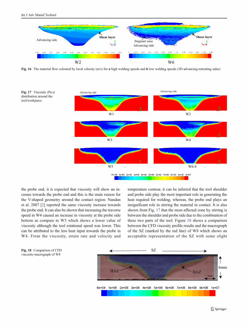
the probe end, it is expected that viscosity will show an in-crease towards the probe end and this is the main reason forthe V-shaped geometry around the contact region. Nandanet al. 2007 [2] reported the same viscosity increase towardsthe probe end. It can also be shown that increasing the traversespeed in W4 caused an increase in viscosity at the probe sidebottom as compare to W3 which shows a lower value ofviscosity although the tool rotational speed was lower. Thiscan be attributed to the less heat input towards the probe inW4. From the viscosity, strain rate and velocity and

temperature contour, it can be inferred that the tool shoulderand probe side play the most important role in generating theheat required for welding, whereas, the probe end plays aninsignificant role in stirring the material in contact. It is alsoshown from Fig. 17 that the most affected zone by stirring isbetween the shoulder and probe side due to the combination ofthese two parts of the tool. Figure 18 shows a comparisonbetween the CFD viscosity profile results and the macrographof the SZ (marked by the red line) of W8 which shows anacceptable representation of the SZ with some slight

W2 W6

Stagnant zone

Advancing side

Advancing side Shear layerShear layer

Fig. 16 The material flow coloured by local velocity (m/s) for a high welding speeds and b low welding speeds (3D advancing-retreating sides)

W1 W2

W3 W4

W5 W6-8

Advancing side Advancing side Fig. 17 Viscosity (Pa.s)distribution around thetool/workpiece

SZ

6mmHAZ HAZ

3mm

Fig. 18 Comparison of CFDviscosity-macrograph of W8

Int J Adv Manuf Technol

differences which may be caused by variation in plunge depthas discussed previously. Figure 18 shows a top view of the

local viscosity for the SZ ofW2 andW6 low and highweldingspeeds respectively. From Figs. 17 and 19, it can be confirmed

W2 W6

Advancing Advancing

Trailing TrailingFig. 19 Local values of viscosity(Pa.s) on the top surface of the SZfor low and high welding speeds(W2 and W6), respectively

Max. shear stress 400 MPa in

shoulder periphery because of high

traverse speed

Advancing Advancing

Trailing Trailing

TrailingTrailing

Advancing Advancing

W3 W4

W5 W6

W1 W2

Trailing Trailing

Advancing Advancing

Max. shear stress in probe sides and

shoulder periphery because of low

temperatures and high viscosity

100MPa150MPa

300MPa 200MPa

Fig. 20 Predicted shear stress(Pa) contours on the tool surface(W1–W6)

Int J Adv Manuf Technol

that the value of viscosity in which material can flow for allcases under study is ranged from 55,000 to 9.8 × 106 Pa.s. Thecutoff viscosity value is 9.8 × 106 Pa.s which is in good agree-ment with the previous work carried out on steel extrusion [2].

4.9 Shear stress on the surface of the tool

The maximum shear stress predicted by the model for low andmedium welding speeds (W1, W2, W3 and W4) as shown inFig. 20 is associated with the leading edge of the tool towardsthe retreating side; which coincides with the prediction for theminimum temperature on the tool (see Fig. 7). The reason forthis is the tool surface leading edge is in contact with higherdegrees of viscosity than the trailing edge as shown in Fig. 18W2. High tool rotational speeds W5 and W6 show a nearlysymmetrical shear stress distribution on the tool shoulder pe-riphery. For constant traverse speeds (W4, W5, and W6), themodel predicts that the shear stress will decrease with increas-ing tool rotational speed because of the associated increase intemperature. The model further predicts that the probe sides issubjected to a higher shear stress at lower tool rotationalspeed, as shown for W1 and W2 in Fig. 20 because it experi-ences lower temperatures and higher viscosity (Fig. 9 andFig. 17, respectively). W4 predicts an increase in shear stressat the shoulder periphery and probe side leading edge com-pared to W3 because of the higher traverse speed. From theprevious discussion, it is recommended to increase the toolrotational speed and decrease the traverse speed in order toreduce the tool wear especially at the probe side and shoulderperiphery.

5 Conclusion

From the preceding discussion, the following can beconcluded:

CFD modelling of FSWof DH36 steel shows that the max-imum temperatures for low and medium welding speeds arelocated under the tool shoulder.

For high rotational speeds (with traverse speed of 400 mm/min) W5 and W6, higher temperatures existed in the shearlayer just out the tool shoulder periphery.

The prediction from the CFD model indicates that com-pared to tool traverse speed, tool rotational speed plays a sig-nificant role in generating heat in the tool/workpiece interface.On the other hand, increasing traverse speed can significantlycause an increase in the cooling rate.

The model predicts that the FSW tool has experienced arange of temperatures across its surface during FSW, a maxi-mum temperature on the advancing-trailing side and a lowertemperature on the leading-retreating side. The minimum tem-perature was found at the probe end.

The CFD model predicts that strain rate increases withincreasing tool rotational speed; it also showed an increasewith increasing traverse speed.

Local pressure between the tool and the workpiece wasasymmetrical between the advancing and retreating sides,the difference in pressure value increases with increasing tra-verse speed.

It is proposed that the increase in pressure difference be-tween the adjacent regions especially near the probe end couldbe the cause of weld defects. High traverse speed may create astagnant zone which in turn can become a source of defectssuch as wormholes as results of the lack in material flowing.

The shape and dimensions of the stirred zone has beenestimated effectively from the viscosity contours in the CFDmodel. The SZ size increased with the increase in tool rota-tional speed. This was because of a decrease in viscositywhich in turn encourages steel layers to rotate.

Viscosity increases with increasing traverse speed especial-ly on the probe side.

The tool shoulder surface experiences high shear stress atlow tool rotational speeds.

The shear stress on the leading-retreating side was greaterthan on the advancing-trailing side because of the temperaturedifference which was lower at the leading-retreating side.

The tool probe sides experience the maximum shear stressat lower tool rotational speeds. The shear stress was also in-creased with increasing the weld traverse speed (e.g. W4).

Acknowledgements The authors would like to thank the TWI compa-ny for providing samples and data of FSW DH36 steel. The author alsothanks the ministry of higher education/Iraq for funding the study. Theauthors are grateful for Ali Riza, the PhD student for his support regardingCFD modelling.

Open Access This article is distributed under the terms of the CreativeCommons At t r ibut ion 4 .0 In te rna t ional License (h t tp : / /creativecommons.org/licenses/by/4.0/), which permits unrestricted use,distribution, and reproduction in any medium, provided you give appro-priate credit to the original author(s) and the source, provide a link to theCreative Commons license, and indicate if changes were made.

References

1. Xiaocong H, Fengshou G, AndrewB (2014) A review of numericalanalysis of friction stir welding. Prog Mater Sci 65:1–66

2. Nandan R, Roy GG, Lienert TJ, Debroy T (2007) Three-dimensional heat and material flow during friction stir welding ofmild steel. Acta Mater 55(3):883–895

3. Toumpis AI, Gallawi A, Arbaoui L, Poletz N (2014) Thermo-mechanical deformation behaviour of DH36 steel during frictionstir welding by experimental validation and modelling. SciTechnol Weld Join 19(8):653–663

4. Micallef D, Camilleri D, Toumpis A, Galloway A, & Arbaoui L(2015) Local heat generation and material flow in friction stirwelding of mild steel assemblies. J Materials: Design andApplications, 0(0)(0), 1–17

Int J Adv Manuf Technol

5. Enkhsaikhan B, Edward C (2009) Detecting wormholes in frictionstir welds from welding feedback data, Midwest instruction andcomputing symposium. South Dakota, USA

6. Toumpis A, Gallawi A, Cater S,McPherson N (2014)Developmentof a process envelope for friction stir welding of DH36 steel—a stepchange. Mater Des 62:64–75

7. Stevenson R, Toumpis A, Galloway A (2015) Defect tolerance offriction stir welds in DH36 steel. Material and design 87:701–711

8. Toumpis AI, Gallawi A, Molter L, Polezhayeva H (2015)Systematic investigation of the fatigue performance of a frictionstir welded low alloy steel. Mater Des 80:116–128

9. Lenard J, Pietrzyk M, Cser L (1999) Mathematical and physicalsimulation of the properties of hot rolled products. Elsevier,Amsterdam, pp 1–10

10. Megastir (2013) Friction Stir Welding of high melting temperaturematerials .Online resource

11. Endo R, Shima M, Susa M (2010) Thermal-conductivity measure-ments and predictions for Ni–Cr solid solution alloys. Int JThermophys 31:1991–2003

12. Atharifar H, Lin D, Kovacevic R (2009) Numerical and experimen-tal investigations on the loads carried by the tool during friction stirwelding. J Mater Eng Perform 18(4):339–350

13. Jacquin D, de Meester B, Simar A, Deloison D, Montheillet F,Desrayaud C (2011) A simple Eulerian thermomechanical model-ing of friction stir welding. J Mater Process Technol 211(1):57–65

14. Grujicic M, Arakere G, Yalavarth HV, He CF, Yen C-F, CheesemanBA (2010) Modeling of AA5083 material-microstructure evolutionduring butt friction-stir welding. J Mater Eng Perform 19(5):672–684

15. Schmidt H (2004) Hattel J and wert J,2004, an analytical model forthe heat generation in friction stir welding. Modelling Simul MaterSci Eng 12:143–157

16. Cox C, Lammlein D, Strauss A, Cook G (2010) Modeling thecontrol of an elevated tool temperature and the affects on axial forceduring friction stir welding. Mater Manuf Process 25:1278–1282

17. Hasan AF, Bennett CJ, Shipway PH (2015) A numerical compari-son of the flow behaviour in friction stir welding (FSW) usingunworn and worn tool geometries. Mater Des 87:1037–1046

18. Al-moussawi M, Smith AJ, Young A, Cater S and Faraji M (2016)An advanced numerical model of friction stir welding of DH36steel, 11th Int. Symp. FSW, TWI Granta Park Cambridge, UK

19. Cho H, Kimd D, Hong S, Jeong Y, Lee K, Cho Y, Kang S, Han H(2015) Three-dimensional numerical model considering phasetransformation in friction stir welding of steel. Metall Mater TransA 46A:6040–6051

20. Arora A, Nandan R, Reynold AP, DebRoya T (2009) Torque, pow-er requirement and stir zone geometry in friction stir weldingthrough modelling and experiments. Scr Mater 60(1):13–16

21. Darvazi AR, Iranmanesh M (2014) Thermal modeling of frictionstir welding of stainless steel 304 L. Int J AdvManuf Technol 75(9–12):1299–1307

22. Pal S, Phaniraj MP (2015) Determination of heat partition betweentool and workpiece during FSW of SS304 using 3D CFD model-ling. J Mater Process Technol 222:280–286

23. Bergman TL, Incropera FP, DeWitt David P, Lavine AS (2011)Fundamentals of heat and mass transfer, 7th E edn. John Wileyand sons, USA

24. Khandkar MZH, Khan JA, Reynolds AP (2003) Prediction of tem-perature distribution and thermal history during friction stirwelding: input torque based model. Sci Technol Weld Join 8(3):165–174

25. Long T, Tang W, Reynolds AP (2007) Process response parameterrelationships in aluminium alloy friction stir welds. Sci TechnolWeld Join 12(4):311–317

26. Elbanhawy A, Chevallier E, Domin K (2013) Numerical investiga-tion of friction stir welding of high temperature materials.NAFEMS world congress, Salzburg

27. Besharati-Givi MK and Asadi P (2014) Advances in friction-stirwelding and processing, a volume in woodhead publishing seriesin welding and other joining technologies, ScienceDirect

28. Fehrenbacher A, Schmale JR, Zinn MR, Pfefferkorn FE (2014)Measurement of tool-workpiece Interface temperature distributionin friction stir welding. J Manuf Sci Eng 136(2):21009

29. Yang KY, Dong H, Kou S (2008) Liquation tendency and liquid-film formation in friction stir spot welding. Weld J 87:202–211

30. Colegrove P, Shercliff (2005) 3-dimensional CFD modelling offlow round a threaded friction stir welding tool profile, H. J MaterProcess Technol 169:320–327

31. Smith AJ, AL-Moussawi M, Young AE, Cater S and Faraji M(2016). Modelling of friction stir welding of 304 stainless steel.In: European Simulation and Modelling Conference, Univ. of LasPalmas, 26-28th October 2016

32. Leonard ES (1999) Light microscopy of carbon steel, ASMInternational ©, USA

33. Wang H, Colegrove PA, dos Santos J (2013) Hybrid modelling of7449-T7 aluminium alloy friction stir welded joints. Sci TechnolWeld Join 18:147–153

34. Fairchild D, Kumar A , Ford S, Nissley N (2009) Researchconcerning the friction stir welding of linepipe steels, Trends inwelding research, Proceedings of the 8th InternationalConference, pp371–380

35. Nandan R, Lienert TJ, Debroy T (2008) Toward reliable calcula-tions of heat and plastic flow during friction stir welding of Ti-6Al-4 V alloy. Int J Mat Res 99(4):434–444

36. Morisada Y, Fujii H, Kawahito Y, Nakata K, Tanaka M (2011)2011, three-dimensional visualization of material flow during fric-tion stir welding by two pairs of X-ray transmission systems. ScrMater 65:1085–1088

37. Schmidt HNB, Dickerson TL, Hattel JH (2006) Material flow inbutt friction stir welds in AA2024-T3. Acta Mater 54:1199–1209

38. MorisadaYet al (2014) Three-dimensional visualization ofmaterialflow during friction stir welding of steel and aluminum. JMater EngPerform 23(11):4143–4147

Int J Adv Manuf Technol