Modelling market risk in extremely low

interest rate environment

The Actuarial Society of Hong Kong

Eric Yau

Consultant, Barrie & Hibbert Asia

Eric.Yau@barrhibb.com

12th Appointed Actuaries Symposium, 7 November 2012

1

Agenda

• Low interest rate…but can it go even lower?

• Monitor your portfolio

• Technical modeling aspects

– Constructing the current yield curve: key assumptions and impact

– Projecting interest rate: stylized facts to consider

2

Can rates go even lower?

3

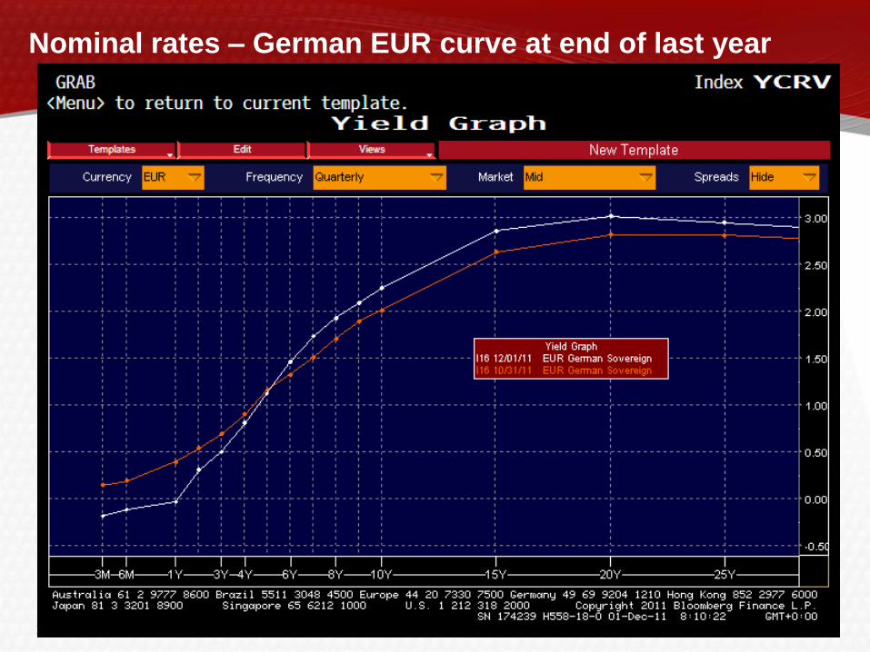
Nominal rates – German EUR curve at end of last year

4

How low can it go

• Traditional axiom of nominal interest rate modelling:

“interest rates are bounded below at zero”

– Closely related to approaches that model shocks as proportional to rate levels

• However,

– US short term rates have gone negative at some points since 2008

• End 2008, March 26th 2009, January 27th 2010, August 4th 2011

– Swiss and German yields have also gone negative

• Two views:

– 1) Very short rates can move to be effectively zero, we might want to model a

point probability of rates hitting zero

– 2) Negative rates are a potential future CB policy (?), therefore we would want

to model a significant probability of negative yield curves

5

Impact of interest rate

on balance sheet

6

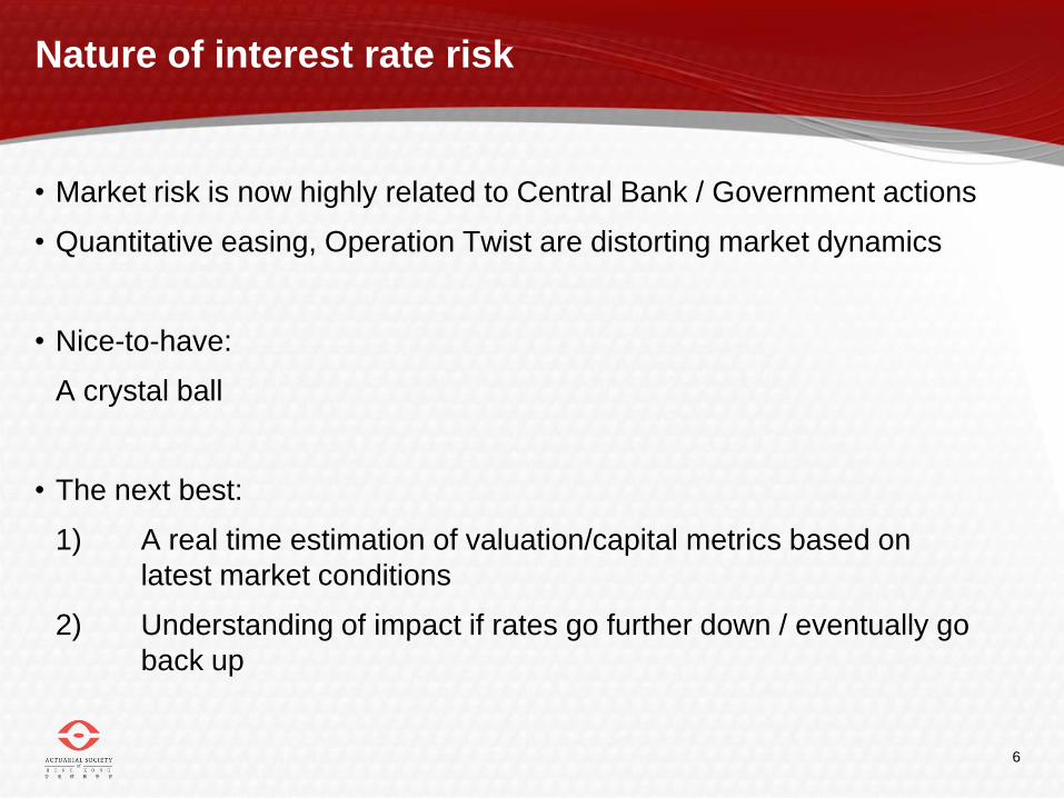
Nature of interest rate risk

• Market risk is now highly related to Central Bank / Government actions

• Quantitative easing, Operation Twist are distorting market dynamics

• Nice-to-have:

A crystal ball

• The next best:

1) A real time estimation of valuation/capital metrics based on

latest market conditions

2) Understanding of impact if rates go further down / eventually go

back up

7

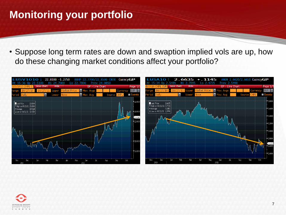
Monitoring your portfolio

• Suppose long term rates are down and swaption implied vols are up, how

do these changing market conditions affect your portfolio?

8

Quick revaluation of liabilities when markets move

A number of ways to achieve this:

• Rerun your models every day / week

– Impractical for most

• Ask what-if questions (“stress testing”)

– Need to ask the right questions!

• Imagine your liabilities behave like assets (“replicating asset”)

– “Good” replicating assets are hard to find

• Describe your liabilities using a function (“curve fitting / LSMC”)

– Curve fitting, Least Square Monte Carlo are sometimes hard to understand

initially

9

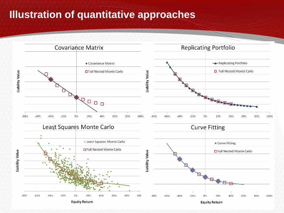
Illustration of quantitative approaches

9

10

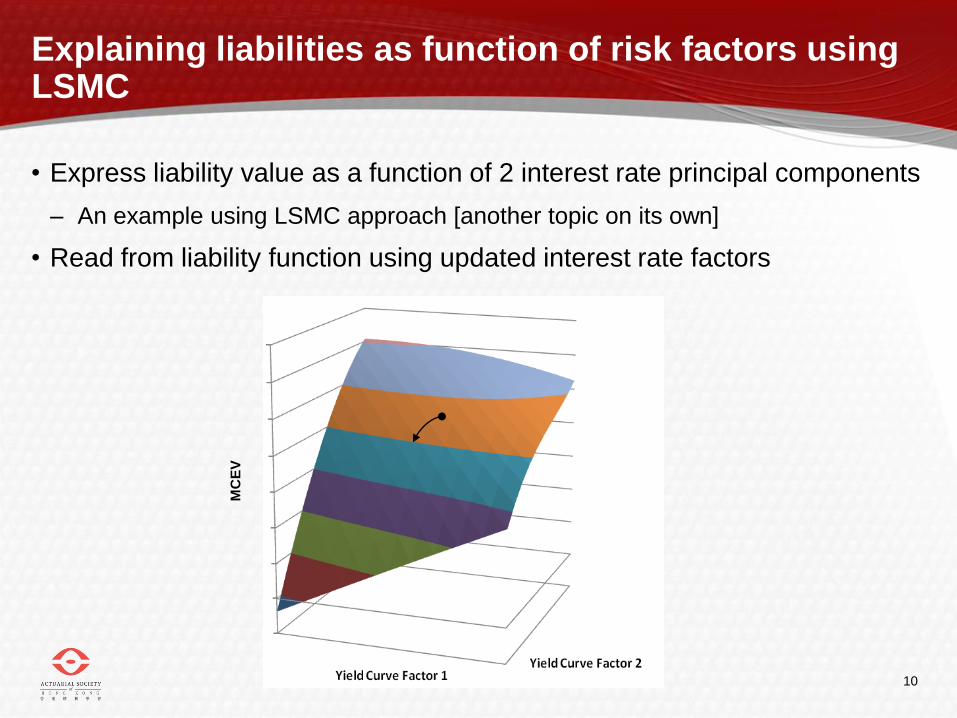
Explaining liabilities as function of risk factors using LSMC

• Express liability value as a function of 2 interest rate principal components

– An example using LSMC approach [another topic on its own]

• Read from liability function using updated interest rate factors

MC

EV

11

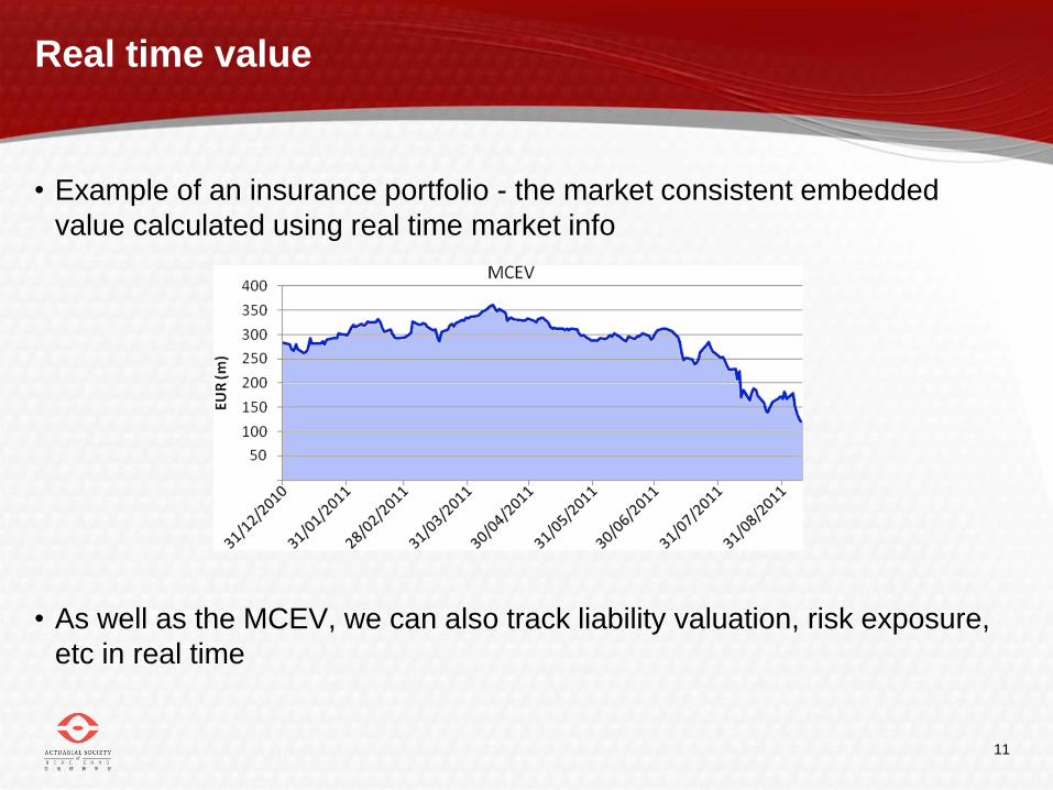
Real time value

• Example of an insurance portfolio - the market consistent embedded

value calculated using real time market info

• As well as the MCEV, we can also track liability valuation, risk exposure,

etc in real time

12

Constructing the initial yield curve

13

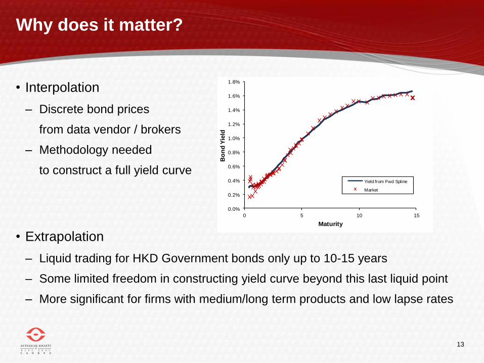
Why does it matter?

• Interpolation

– Discrete bond prices

from data vendor / brokers

– Methodology needed

to construct a full yield curve

• Extrapolation

– Liquid trading for HKD Government bonds only up to 10-15 years

– Some limited freedom in constructing yield curve beyond this last liquid point

– More significant for firms with medium/long term products and low lapse rates

0.0%

0.2%

0.4%

0.6%

0.8%

1.0%

1.2%

1.4%

1.6%

1.8%

0 5 10 15

Bo

nd

Yie

ldMaturity

Yield from Fwd Spline

Market

14

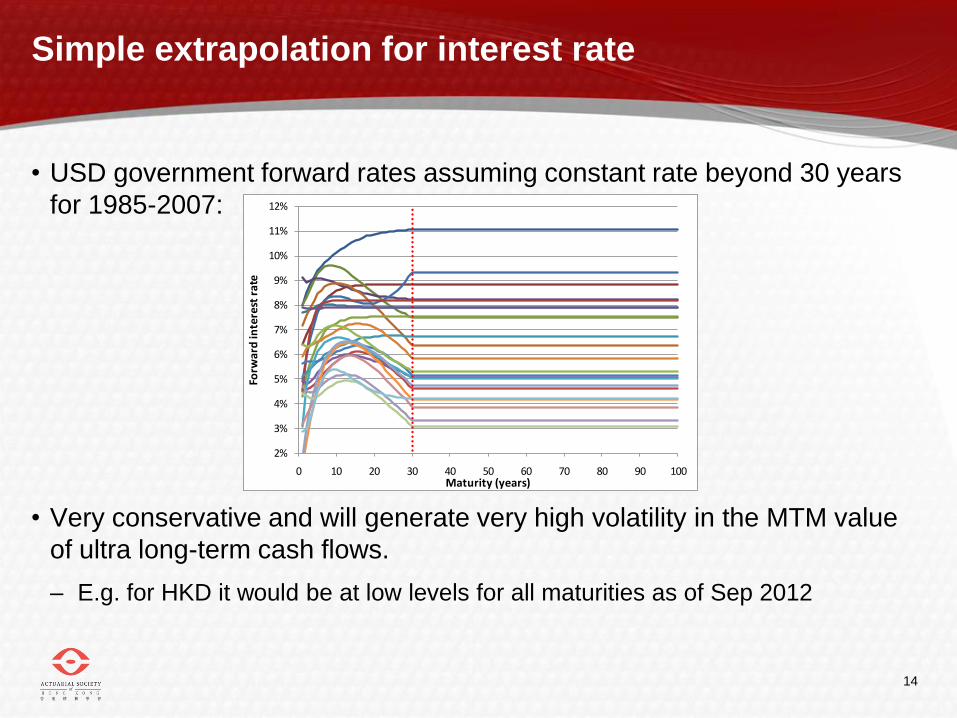
Simple extrapolation for interest rate

• USD government forward rates assuming constant rate beyond 30 years

for 1985-2007:

• Very conservative and will generate very high volatility in the MTM value

of ultra long-term cash flows.

– E.g. for HKD it would be at low levels for all maturities as of Sep 2012

2%

3%

4%

5%

6%

7%

8%

9%

10%

11%

12%

0 10 20 30 40 50 60 70 80 90 100

Forw

ard

inte

rest

rat

e

Maturity (years)

15

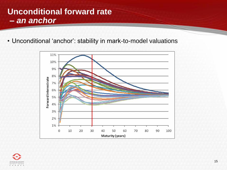
Unconditional forward rate – an anchor

• Unconditional ‘anchor’: stability in mark-to-model valuations

16

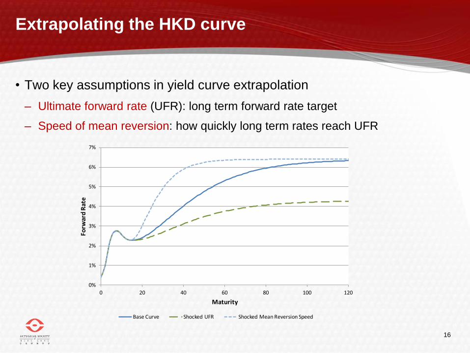
Extrapolating the HKD curve

• Two key assumptions in yield curve extrapolation

– Ultimate forward rate (UFR): long term forward rate target

– Speed of mean reversion: how quickly long term rates reach UFR

0%

1%

2%

3%

4%

5%

6%

7%

0 20 40 60 80 100 120

Forw

ard

Rat

e

Maturity

Base Curve Shocked UFR Shocked Mean Reversion Speed

17

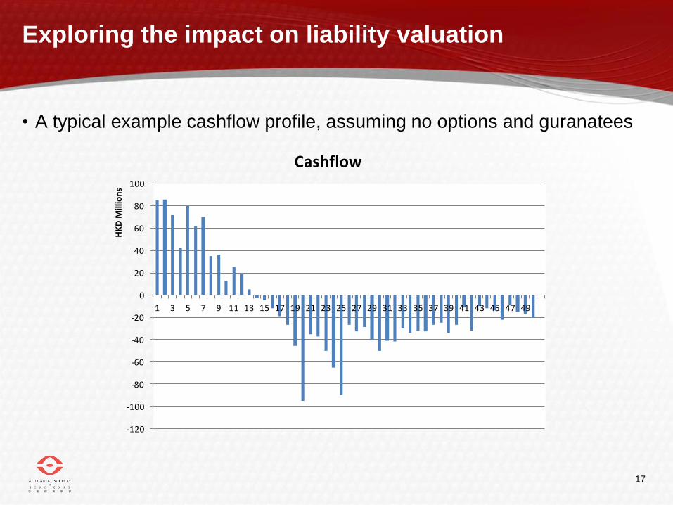
Exploring the impact on liability valuation

• A typical example cashflow profile, assuming no options and guranatees

-120

-100

-80

-60

-40

-20

0

20

40

60

80

100

1 3 5 7 9 11 13 15 17 19 21 23 25 27 29 31 33 35 37 39 41 43 45 47 49

HK

D M

illio

ns

Cashflow

18

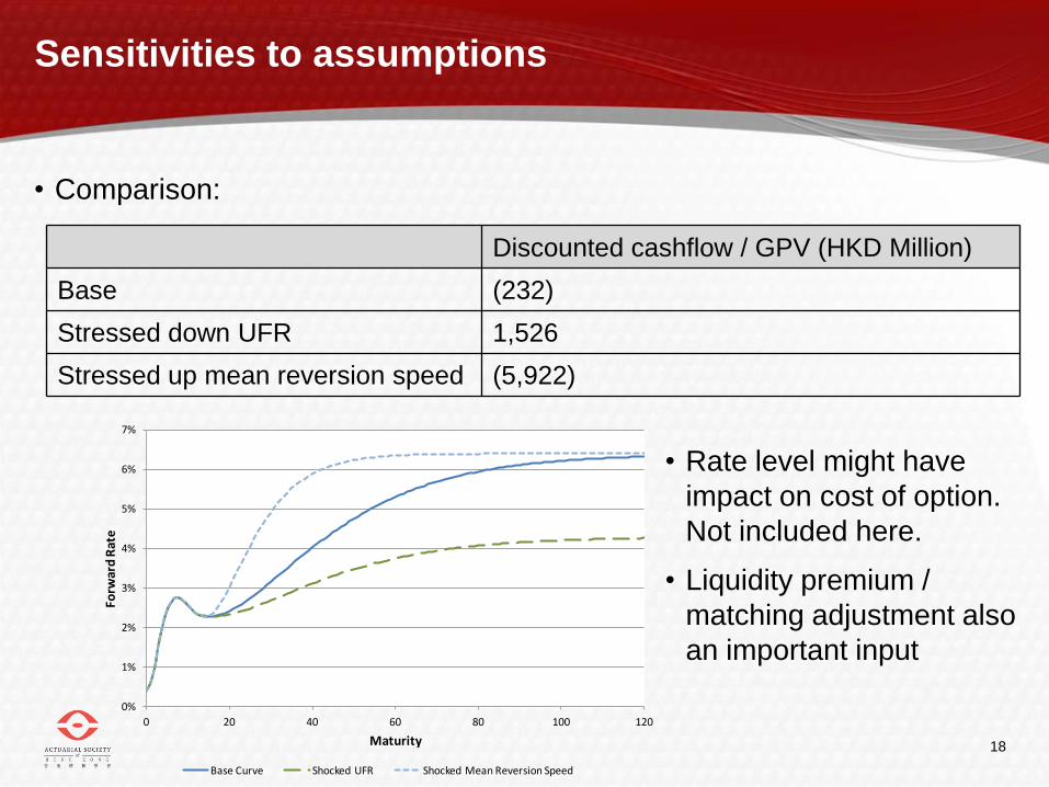
Sensitivities to assumptions

• Comparison:

Discounted cashflow / GPV (HKD Million)

Base (232)

Stressed down UFR 1,526

Stressed up mean reversion speed (5,922)

0%

1%

2%

3%

4%

5%

6%

7%

0 20 40 60 80 100 120

Forw

ard

Rat

e

Maturity

Base Curve Shocked UFR Shocked Mean Reversion Speed

• Rate level might have

impact on cost of option.

Not included here.

• Liquidity premium /

matching adjustment also

an important input

19

Modeling future interest rate

movement

20

Some stylized facts

• Interest rates are mean reverting

– Justification for using mean reverting model

• Long term expectations are stable

– Useful for setting ultimate forward rate target (UFR)

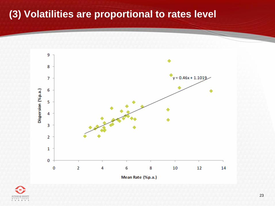
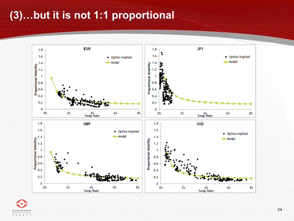
• Volatilities are proportional to rates level, but not 1:1

– Vols determine how wide the ranges are and hence VaR

– Cost of guarantee driven by both level of rates and vols

21

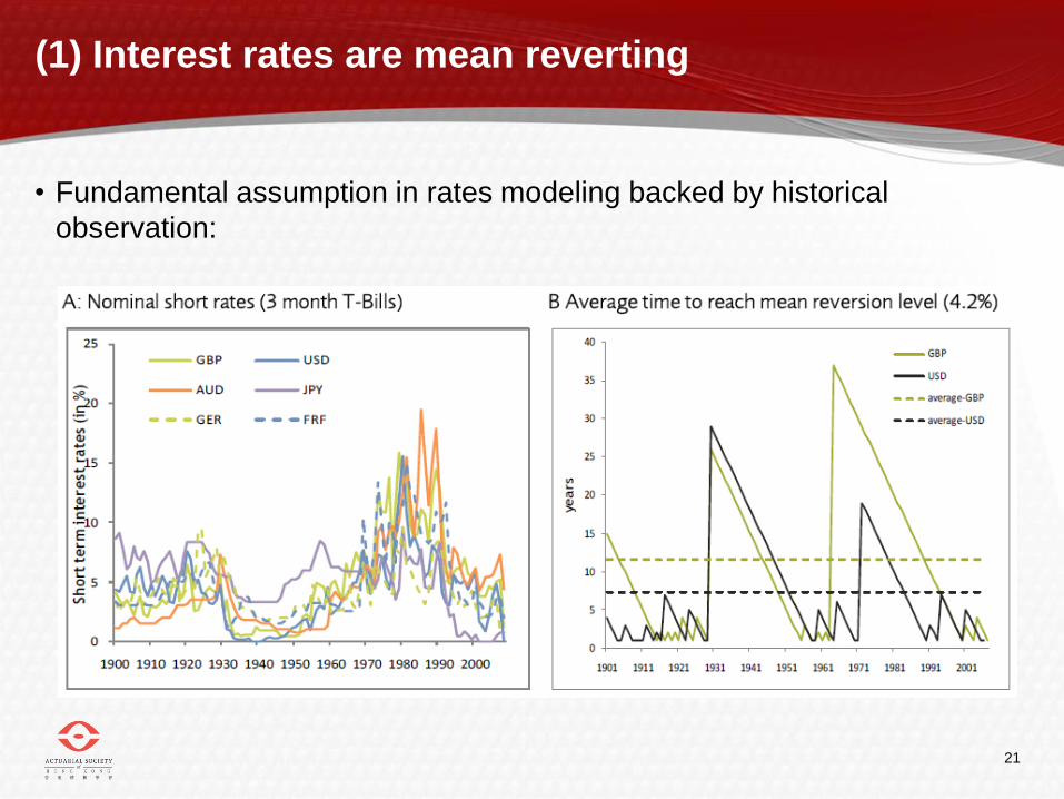
(1) Interest rates are mean reverting

• Fundamental assumption in rates modeling backed by historical

observation:

22

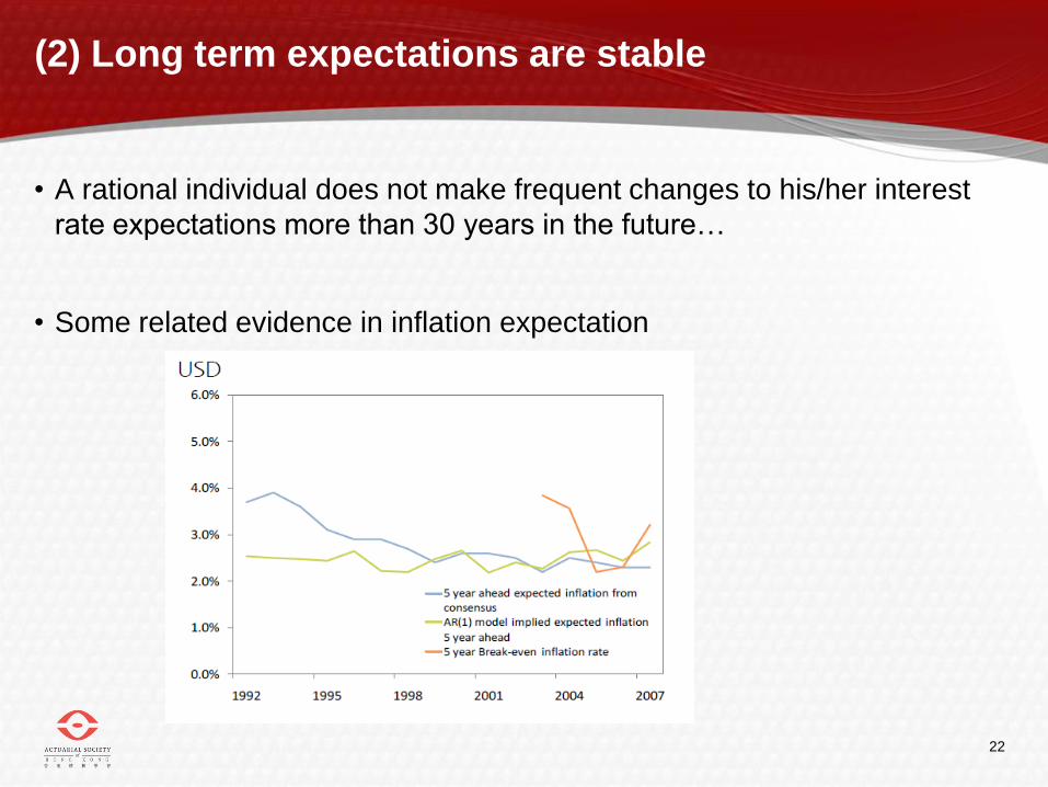
(2) Long term expectations are stable

• A rational individual does not make frequent changes to his/her interest

rate expectations more than 30 years in the future…

• Some related evidence in inflation expectation

23

(3) Volatilities are proportional to rates level

24

(3)…but it is not 1:1 proportional

25

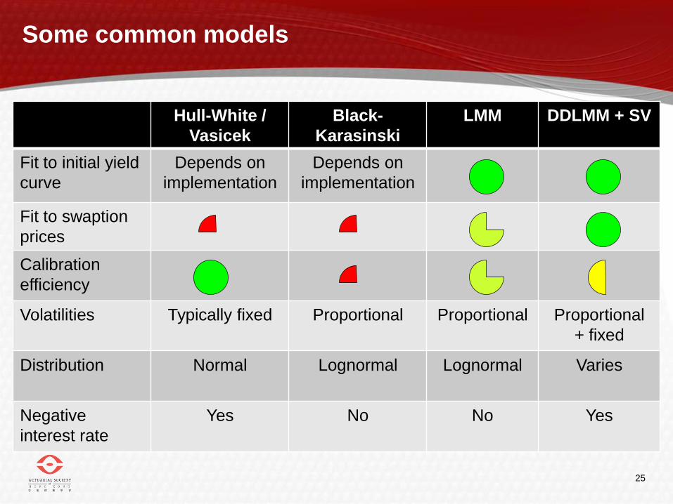
Some common models

Hull-White /

Vasicek

Black-

Karasinski

LMM DDLMM + SV

Fit to initial yield

curve

Depends on

implementation

Depends on

implementation

Fit to swaption

prices

Calibration

efficiency

Volatilities Typically fixed Proportional Proportional Proportional

+ fixed

Distribution Normal Lognormal Lognormal Varies

Negative

interest rate

Yes No No Yes

26

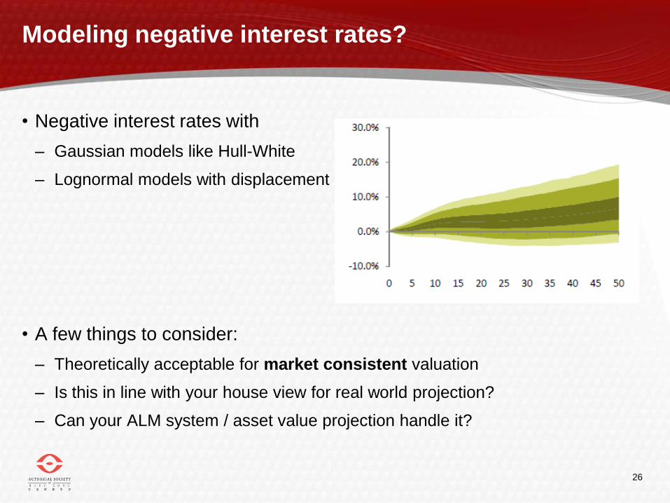
Modeling negative interest rates?

• Negative interest rates with

– Gaussian models like Hull-White

– Lognormal models with displacement

• A few things to consider:

– Theoretically acceptable for market consistent valuation

– Is this in line with your house view for real world projection?

– Can your ALM system / asset value projection handle it?

27

Concluding remarks

• Prediction vs probability distribution

• Observing stylized facts in the markets and reflecting them in the models

• Understanding sensitivities of your liabilities

28

Thank you!

Technical appendix

30

Calibration

31

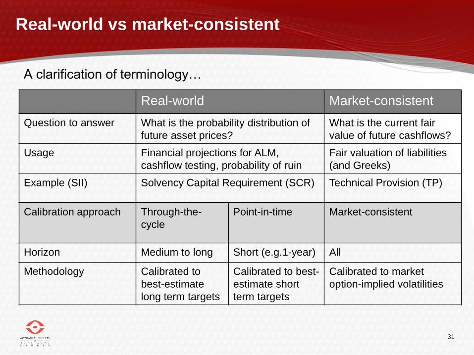
A clarification of terminology…

Real-world vs market-consistent

Real-world Market-consistent

Question to answer What is the probability distribution of

future asset prices?

What is the current fair

value of future cashflows?

Usage Financial projections for ALM,

cashflow testing, probability of ruin

Fair valuation of liabilities

(and Greeks)

Example (SII) Solvency Capital Requirement (SCR) Technical Provision (TP)

Calibration approach Through-the-

cycle

Point-in-time Market-consistent

Horizon Medium to long Short (e.g.1-year) All

Methodology Calibrated to

best-estimate

long term targets

Calibrated to best-

estimate short

term targets

Calibrated to market

option-implied volatilities

32

Challenges in risk factor modelling

• Consistency of calibration approach across diverse range of risk factors

– Different types of model processes, different data availability

• Documentation and validation, especially in areas of expert judgement

– Limitations of volume and relevance of historical data for calibration and

validation of 1-year 99.5th percentile

• Definition of the 1-year risk measure:

– Through-the-Cycle and Point-in-Time probability definitions

• e.g. If calibrating the Internal Model today:

– How much mean-reversion is it reasonable to assume will, on average, occur to

interest rates over next 12 months? More than implied by current forward rates?

– Should 1-year equity volatility assumption reflect unusual economic

environment and the current high levels of market volatility?

33

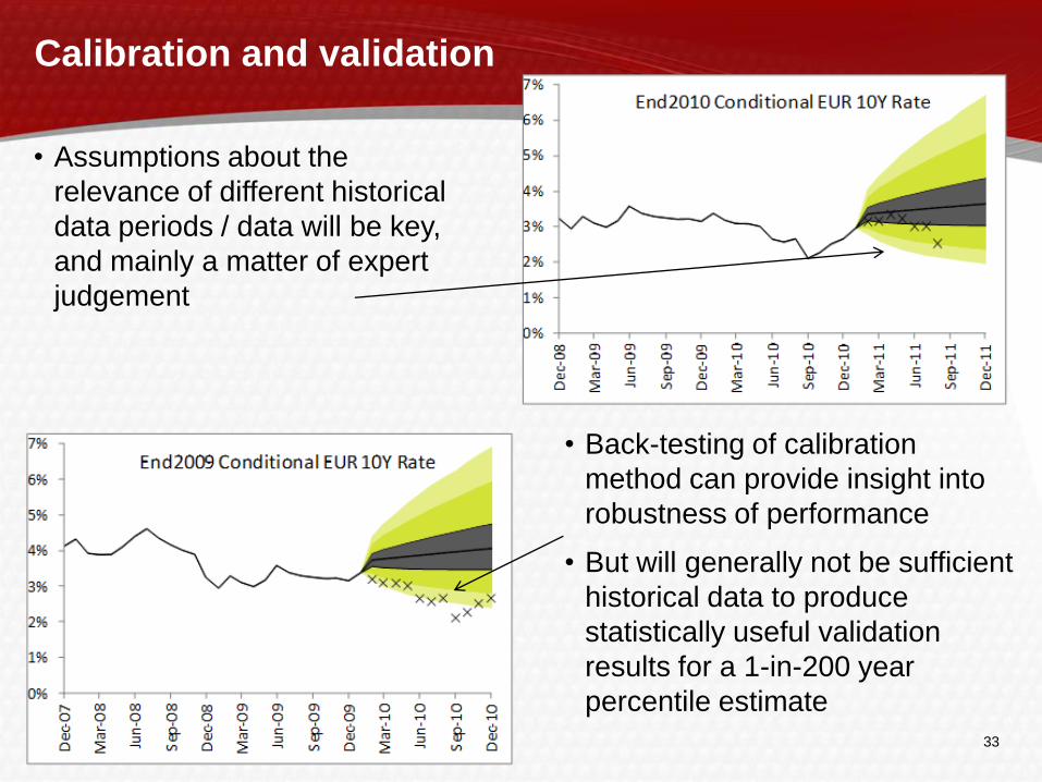
Calibration and validation

• Back-testing of calibration

method can provide insight into

robustness of performance

• But will generally not be sufficient

historical data to produce

statistically useful validation

results for a 1-in-200 year

percentile estimate

• Assumptions about the

relevance of different historical

data periods / data will be key,

and mainly a matter of expert

judgement

34

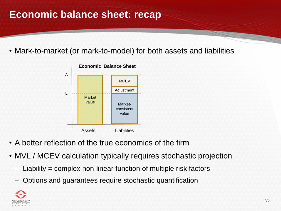
Economic balance sheet

35

Economic balance sheet: recap

• Mark-to-market (or mark-to-model) for both assets and liabilities

• A better reflection of the true economics of the firm

• MVL / MCEV calculation typically requires stochastic projection

– Liability = complex non-linear function of multiple risk factors

– Options and guarantees require stochastic quantification

Market

value Market-

consistent

value

Assets Liabilities

Economic Balance Sheet

A

L

MCEV

Adjustment

36

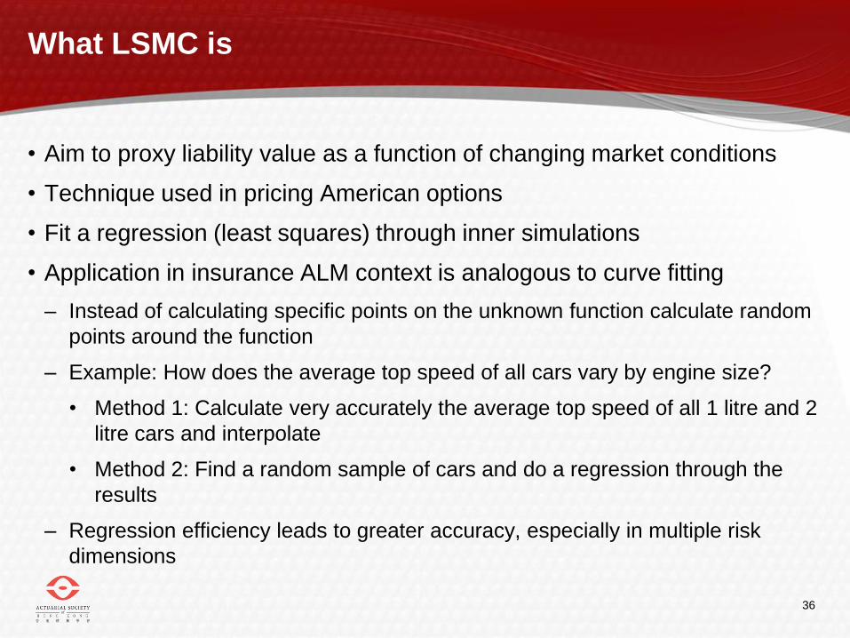
What LSMC is

• Aim to proxy liability value as a function of changing market conditions

• Technique used in pricing American options

• Fit a regression (least squares) through inner simulations

• Application in insurance ALM context is analogous to curve fitting

– Instead of calculating specific points on the unknown function calculate random

points around the function

– Example: How does the average top speed of all cars vary by engine size?

• Method 1: Calculate very accurately the average top speed of all 1 litre and 2

litre cars and interpolate

• Method 2: Find a random sample of cars and do a regression through the

results

– Regression efficiency leads to greater accuracy, especially in multiple risk

dimensions

37

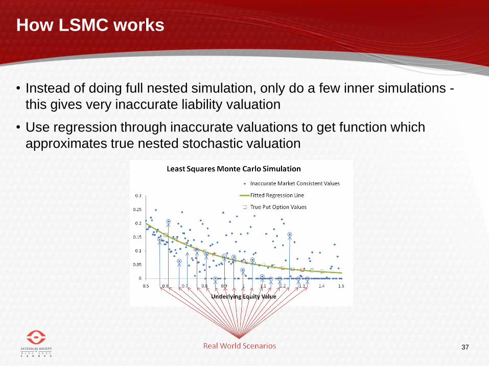
How LSMC works

• Instead of doing full nested simulation, only do a few inner simulations -

this gives very inaccurate liability valuation

• Use regression through inaccurate valuations to get function which

approximates true nested stochastic valuation

38

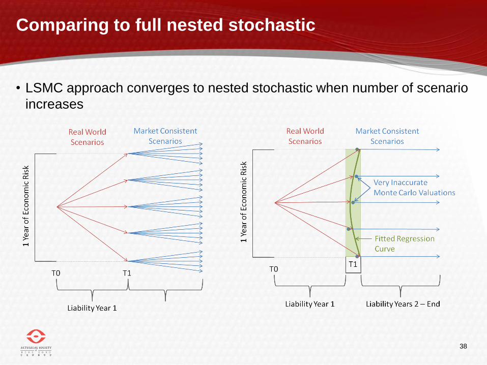
Comparing to full nested stochastic

• LSMC approach converges to nested stochastic when number of scenario

increases

39

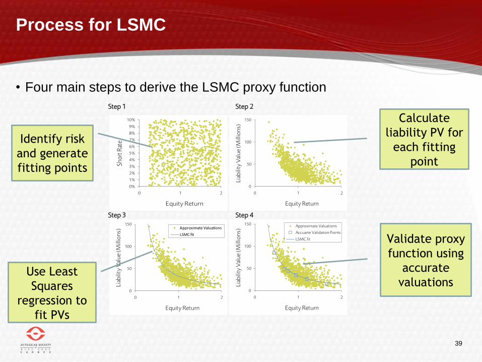
Process for LSMC

• Four main steps to derive the LSMC proxy function

Step 1 Step 2

Step 3 Step 4

0%

1%

2%

3%

4%

5%

6%

7%

8%

9%

10%

0 1 2

Sh

ort

Rat

e

Equity Return

0

50

100

150

0 1 2

Lia

bili

ty V

alu

e (

Mill

ion

s)

Equity Return

0

50

100

150

0 1 2

Lia

bili

ty V

alu

e (

Mill

ion

s)

Equity Return

Approximate Valuations

LSMC fit

0

50

100

150

0 1 2

Lia

bili

ty V

alu

e (

Mill

ion

s)

Equity Return

Approximate Valuations

Accuarte Validation Points

LSMC fit

Identify risk

and generate

fitting points

Use Least

Squares

regression to

fit PVs

Calculate

liability PV for

each fitting

point

Validate proxy

function using

accurate

valuations

40

Copyright 2012 Barrie & Hibbert Limited. All rights reserved. Reproduction in whole or in part is

prohibited except by prior written permission of Barrie & Hibbert Limited (SC157210) registered in Scotland

at 7 Exchange Crescent, Conference Square, Edinburgh EH3 8RD.

The information in this document is believed to be correct but cannot be guaranteed. All opinions and

estimates included in this document constitute our judgment as of the date indicated and are subject to

change without notice. Any opinions expressed do not constitute any form of advice (including legal, tax

and/or investment advice). This document is intended for information purposes only and is not intended as

an offer or recommendation to buy or sell securities. The Barrie & Hibbert group excludes all liability

howsoever arising (other than liability which may not be limited or excluded at law) to any party for any loss

resulting from any action taken as a result of the information provided in this document. The Barrie & Hibbert

group, its clients and officers may have a position or engage in transactions in any of the securities

mentioned.

Barrie & Hibbert Inc. and Barrie & Hibbert Asia Limited (company number 1240846) are both wholly owned

subsidiaries of Barrie & Hibbert Limited.

www.barrhibb.com